Resolving Galactic binaries in LISA data using particle swarm optimization and cross-validation

Abstract

The space-based gravitational wave (GW) detector LISA is expected to observe signals from a large population of compact object binaries, comprised predominantly of white dwarfs, in the Milky Way. Resolving individual sources from this population against its self-generated confusion noise poses a major data analysis problem. We present an iterative source estimation and subtraction method to address this problem based on the use of particle swarm optimization (PSO). In addition to PSO, a novel feature of the method is the cross-validation of sources estimated from the same data using different signal parameter search ranges. This is found to greatly reduce contamination by spurious sources and may prove to be a useful addition to any multi-source resolution method. Applied to a recent mock data challenge, the method is able to find $O(10^{4})$ Galactic binaries across a signal frequency range of $[0.1,15]$ mHz, and, for frequency $\gtrsim 4$ mHz, reduces the residual data after subtracting out estimated signals to the instrumental noise level.

I Introduction

The gravitational wave (GW) window in the frequency range $[10,10^{3}]$ Hz has now been opened using ground-based detectors: the LIGO [1] and Virgo [2] detectors have observed several binary black hole mergers [3, 4, 5] and one double neutron star merger [6]. Work is in progress to extend this success to lower frequency ranges. The space-based Laser Interferometric Space Antenna (LISA) mission [7], to be launched around $2034$, will probe the $[10^{-4},1]$ Hz band. Key experimental technologies required for LISA have been demonstrated successfully in the LISA Pathfinder mission [8]. LISA may be joined by additional space-based missions currently under study, namely, Taiji [9] and Tianqin [10]. The exploration of the nanohertz frequency range, $[10^{-9},10^{-7}]$ Hz, is well underway using pulsar timing arrays (PTAs) [11], with the sensitivity of these searches expected to increase by orders of magnitude [12] as next-generation radio telescopes [13, 14] come online over the coming decade.

The planned configuration of LISA [7] is a set of three satellites in heliocentric orbits, each one housing freely falling proof masses, that will maintain a triangular formation trailing the Earth by about $20^{\circ}$. At the lowest order of approximation, the triangle is rigid and equilateral with an arm length of $2.5\times 10^{6}$ km. It is tilted with respect to the ecliptic and rotates around its centroid with a period of $1$ year. GW induced fluctuation in the arm lengths will be measured using the technique of time delay interferometry (TDI) [15] that linearly combines time-delayed readouts of frequency shifts in the light exchanged by the satellites. There are several such TDI combinations, of which the so-called A, E, T combinations have mutually uncorrelated instrumental noise.

Since LISA is a nearly omnidirectional detector, GW signals from sources distributed across the sky will appear simultaneously and additively in TDI data. Predominant among these are expected to be long-lived signals from a variety of compact object binaries, including (i) several Massive Black Hole Binaries (MBHBs) [16] with components masses in the $[10^{3},10^{6}]$ $M_{\odot}$ range, (ii) a few extreme mass ratio systems [17] of stellar mass black holes in orbit around massive ones, and (iii) $O(10^{8})$ Galactic binaries (GBs) within the Milky Way comprised primarily of white dwarfs [18].

Disentangling a myriad of signals from multiple sources of different types, i.e., multisource resolution, is a major data analysis problem for LISA. The LISA community has organized a series of challenges to encourage the development of data analysis methods for addressing this humongous task. The first to the fourth of these were called Mock LISA Data Challenges (MLDCs) [19, 20, 21] and the subsequent ones are part of a series called LISA Data Challenge (LDC) [22]. The first LDC (LDC1) consists of several sub-challenges, of which the fourth (LDC1-4) pertains to GB resolution.

While the signal from a GB in its source frame is quite simple in form – a nearly constant amplitude linear chirp with an increasing or decreasing secular frequency drift depending on mass transfer, or lack thereof, between the components – its spectrum is broadened considerably due to the frequency and amplitude modulations imposed by the motion of LISA. The resulting increase in the overlap of the signals, accompanied by their sheer number, makes the GB resolution problem especially challenging. In particular, GBs should be so numerous at low frequencies ($\lesssim 3$ mHz) that the confusion noise from the blending of their signals is expected to dominate the instrumental noise. Thus, not only do individual sources need to be differentiated from each other but they also need to be resolved against the background of confusion noise, with the latter defined by, as well as affecting, the data analysis method used.

Quantifying the performance of multisource resolution methods is not as straightforward as the case of a single source search. The sources found by any method, called reported sources in this paper, will generally consist of some that correspond to true sources while others that do not. Differentiating between them is non-trivial since no reported source will have an exact match, in either its signal waveform or source parameters, with a true source. Past data challenges have employed a test, described in detail later, for this purpose that is based on the cross-correlation of reported and true signal waveforms. In the following, we refer to reported sources that pass such a test as confirmed sources and their number relative to that of reported sources as the detection rate. Note that in some methods, the reported sources themselves may be filtered out from a much larger set of identified sources by applying some cuts to reject spurious sources.

A variety of data analysis methods have been proposed for the GB resolution problem. Some (e.g., [23]) remain proof of principle studies while others were quite mature even by the first data challenge. The methods that have emerged at the top of the pack through the data challenges are as follows. (i)BAM [24] combined simulated annealing and Markov Chain Monte Carlo (MCMC), in a block-wise frequency search to report $\simeq 20,000$ sources in MLDC-2.1 data that had $26$ million GBs. From Fig.1 in [20], we estimate that it achieved a detection rate of $\approx 85\%$. (ii) An extension of BAM [25] incorporating trans-dimensional MCMC was tested on the training data from MLDC-4 and reported $\simeq 9,000$ sources in the $[0,10]$ mHz band with a detection rate of $\simeq 90\%$. (The loss in performance relative to BAM was attributed to an additional signal parameter, namely, the secular frequency drift, that was missing in MLDC-2.1.) (iii) A deterministic search with iterative source subtraction proposed in [26] reported $\simeq 12,000$ sources in MLDC-3.1 data containing $60$ million GBs. (The viability of the deterministic and iterative source subtraction approach for GB resolution was demonstrated earlier in [27].) A new front in GB resolution has been opened recently [28] where the goal is to create a time-evolving source catalog as the data from LISA accumulates. In contrast, the methods listed above use the entire data from a fixed observation period.

In this paper, we introduce a new iterative source subtraction method for the GB resolution problem and demonstrate it on LDC1-4 data as well as data, that we call MLDC-3.1mod, obtained by adding the GBs used in MLDC-3.1 to the noise realizations in LDC1-4. By taking out possible differences in noise characteristics between the two challenges from the equation, the latter allows a more equitable assessment of the effects of the much larger number of sources in MLDC-3.1. Among the key novel features of our method are the use of particle swarm optimization (PSO) [29] for accelerating the baseline task of single source estimation, and the rejection of spurious sources by cross-validating identified sources found with different search ranges for the secular frequency drift parameter. We call the method GBSIEVER: Galactic Binary Separation by Iterative Extraction and Validation using Extended Range.

Depending on the cuts that filter out reported sources from identified ones, the number of reported sources for LDC1-4 data from GBSIEVER falls between $9,291$ and $12,270$ in the $[0.1,15]$ mHz band with an overall detection rate between $91.19\%$ and $84.28\%$, respectively. For MLDC-3.1mod the numbers are $9,387$ and $12,044$ with detection rates of $90.26\%$ and $84.16\%$, respectively. These results are comparable to the ones for the methods listed earlier. The numbers above are just snapshots of an extensive performance analysis of GBSIEVER contained in this paper that also includes an assessment of parameter estimation errors.

The rest of the paper is organized as follows. The challenge data used in this paper are described in Sec. II. The baseline single-source detection and parameter estimation method is described in Sec. III. GBSIEVER is described in Sec. IV, followed by the results in Sec V. Our conclusions and prospects for future work are presented in Sec. VI.

II Challenge data description

We begin with a brief outline of LDC1-4 data, limited to establishing the notation used in the rest of the paper. For a plane GW, with polarizations $h_{+}(t)$ and $h_{\times}(t)$ (in the TT-gauge), emitted by a source located in the Solar System Barycentric (SSB) frame at ecliptic latitude, $\beta$, and ecliptic longitude, $\lambda$, the response of a single arm indexed by $l$ and having length $L$ is,

$$y_{slr}(t) =\frac{\Phi_{l}\left(t^{\prime}-\widehat{k}\cdot\overline{R}_{s}(t^{\prime})\right)-\Phi_{l}\left(t-\widehat{k}\cdot\overline{R}_{r}(t)\right)}{2(1-\widehat{k}\cdot\widehat{n}(t))}\;,$$ (1)

$$\Phi_{l}(t) =\sum_{a=+,\times}F_{a,l}(t;\lambda,\beta,\psi)h_{a}(t)\;,$$ (2)

where, $t^{\prime}=t-L/c$, $\overline{R}_{s}$ and $\overline{R}_{r}$ are, respectively, the SSB frame positions of the satellites (indexed by $s$ and $r$) sending and receiving light along this arm, $\widehat{n}(t)$ is the unit vector along $\overline{R}_{r}(t)-\overline{R}_{s}(t^{\prime})$, $\widehat{k}$ is the unit vector along the GW propagation direction, $F_{+,l}$ and $F_{\times,l}$ are the antenna pattern functions for the arm, and $\psi$ – the polarization angle – defines the orientation of the wave frame axes in the plane orthogonal to $\widehat{k}$. The time dependence of the antenna patterns is induced by the orbital motion of LISA. The GW signal in each TDI combination is obtained by combining the single arm responses with prescribed time delays. (Further details about TDI data generation are in the LDC1 manual [22].)

For a GB, $h_{+,\times}(t)$ are linear chirps,

$$h_{+}(t) =\mathcal{A}\left(1+\cos^{2}\iota\right)\cos\Phi(t)\;,$$ (3)

$$h_{\times}(t) =-2\mathcal{A}\cos\iota\sin\Phi(t)\;,$$ (4)

$$\Phi(t) =\phi_{0}+2\pi ft+\pi\dot{f}t^{2}\;,$$ (5)

that are parametrized by the overall amplitude $\mathcal{A}$, initial phase $\phi_{0}$ at the start of observation, inclination $\iota$ of the GB orbit to the line of sight from the SSB origin, carrier frequency $f$, and secular frequency drift $\dot{f}$. (For a GB, $\psi$ specifies the orientation of the orbit’s projection on the sky.) The majority of GBs in LDC1-4 data have frequencies in the $\approx[0.1,15]$ mHz range, with only 18 having $f>15$ mHz, and the source number density in frequency increases as one moves to lower frequencies.

Fig. 1 illustrates A and E signals, in both the time and Fourier domains, from a single GB. (The T combination is ignored from here on because the GW signal in it is highly attenuated at low frequencies.) The Doppler shift arising from the orbital motion of LISA and the time dependence of its antenna patterns induce periodic modulations in the instantaneous frequency and amplitude of an observed GB signal. Over an observation period $T_{\rm obs}=2$ years, the energy of a GB signal with frequency $f$ (Hz) is spread by Doppler modulation over a frequency range $\Delta f_{\rm dplr}$ that is a factor of $\approx 10^{4}\times f$ larger than $1/T_{\rm obs}$, the minimum spacing of Fourier frequencies. This not only reduces the peak Fourier domain amplitude of GB signals substantially but also increases their overlap, thereby making the problem of resolving them very challenging.

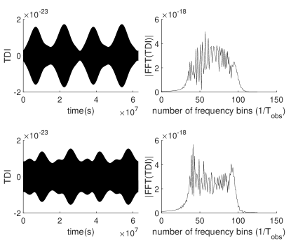
Figure 1: TDI A (top row) and E (bottom row) signals corresponding to a single GB with $f\simeq 5$ mHz and $T_{\rm obs}=2$ yr in (left column) the time and (right column) the Fourier domain. The Fourier frequency is expressed in units of $1/T_{\rm obs}$.

Each TDI combination in LDC1-4 contains the sum of signals from a set of $30$ million GBs drawn randomly from an astrophysically realistic population model [18]. (The corresponding number for MLDC-3.1 is $60$ million.) To this collective signal is added a realization of a pseudo-random sequence that models the instrumental noise. The software, called LISACode [30], that generates LDC TDI data also provides the respective noise realizations. Both LDC1-4 and MLDC-3.1 disclose the true parameters of the GBs used in synthesizing their respective challenge data. We generated the TDI combinations corresponding to the GB parameters in MLDC-3.1 and added them to the LISACode noise realizations. As mentioned in Sec. I, we call the resulting data MLDC-3.1mod.

Fig. 2 compares the distributions of the amplitude parameter in LDC1-4 and MLDC-3.1. Even though the latter has twice the number of sources, the majority of them are low amplitude ones. Hence, one does not expect to resolve a significantly larger number of GBs in MLDC-3.1 (or MLDC-3.1mod). The range of true $\dot{f}$ in these datasets is relevant for the cross-validation step in GBSIEVER: In LDC1-4, $-3.3\times 10^{-17}\lesssim\dot{f}\lesssim 6.8\times 10^{-16}$ ${\rm Hz}^{2}$ for $f<4$ mHz and $-3.0\times 10^{-15}\lesssim\dot{f}\lesssim 3.9\times 10^{-14}$  ${\rm Hz}^{2}$ for $f\in[4,15]$ mHz; In MLDC-3.1, $-3.8\times 10^{-17}\lesssim\dot{f}\lesssim 1.1\times 10^{-15}$ ${\rm Hz}^{2}$ for $f<4$ mHz and $-2.3\times 10^{-14}\lesssim\dot{f}\lesssim 7.7\times 10^{-14}$  ${\rm Hz}^{2}$ for $f\in[4,15]$ mHz.

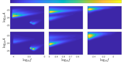
Figure 2: Kernel density estimate of the joint distribution of amplitude, $\mathcal{A}$, and frequency, $f$ (Hz), for LDC1-4 (top row) and MLDC-3.1 (bottom row) sources. The range of values on the Y-axis is the same in each row and shown only for the leftmost column for clarity. The estimated density in each panel is color coded according to the map shown at the top, with values increasing from left to right. The color coding of density values is the same for LDC1-4 and MLDC-3.1 within each column of panels (i.e., frequency interval) but differs across the columns. This allows the extreme values of density that occur in the combined frequency range to be displayed simultaneously.

III F-statistic and its implementation

Each TDI time series in LDC1-4 is uniformly sampled with a sampling interval $\Delta=15$ sec. With $\overline{x}$ denoting a row vector, the data from a TDI combination $I\in\{{\rm A},{\rm E}\}$ is given by

$$\overline{y}^{I} = \overline{S}^{I}+\overline{n}^{I}\;,$$ (6)

where $\overline{S}^{I}$ denotes the collective GW signal from all the GBs, any one of which will be denoted by $\overline{s}^{I}$, and $\overline{n}^{I}$ denotes the instrumental noise realization. For LDC1-4, $\overline{y}^{I}\in\mathbb{R}^{N}$ with $N=4194304$, corresponding to $T_{\rm obs}\approx 2$ yr. The instrumental noise is modeled by a Gaussian, stationary, stochastic process with power spectral density (PSD) $S_{n}^{I}(\nu)$ at Fourier frequency $\nu$.

III.1 Parameter estimation: single source

GBSIEVER uses iterative estimation of signals in which each step estimates the parameters of a GB signal using maximum likelihood estimation (MLE) under the assumption that the data contains only a single source. The estimated signal is subtracted from the data and the process is repeated on the residual. (The formalism for MLE below closely follows the one in [26] to which we refer the reader for more details.)

The GW signal from a single GB can be expressed, schematically, as

$$\overline{s}^{I}(\theta) =\overline{a}\,{\bf X}^{I}(\kappa)\;,$$ (7)

where $\overline{a}=(a_{1},a_{2},a_{3},a_{4})\in\mathbb{R}^{4}$ and ${\bf X}^{I}(\kappa)$ is a $4$-by-$N$ matrix of template waveforms. The former, called the set of extrinsic parameters, is a reparametrization of the four parameters $\mathcal{A}$, $\phi_{0}$, $\psi$, and $\iota$. The latter depends on the remaining set, $\kappa=\{\lambda,\beta,f,\dot{f}\}$, of the so-called intrinsic parameters. The complete set of parameters is denoted by $\theta=\{\overline{a},\kappa\}$. We make a parenthetical remark here that GBSIEVER uses the expressions in [26] for generating template waveforms while the signals in LDC1-4 are generated by the FastGB code [31]. However, we have verified that the two are in good agreement for the A and E combinations in the frequency range of interest here.

The point estimate of the parameters $\theta$ in an iteration is obtained as,

$$\widehat{\theta} =\operatorname*{argmin}_{\theta}\sum_{I\in\{A,E\}}\left(\|\overline{y}^{I}-\overline{s}^{I}(\theta)\|^{I}\right)^{2}\;,$$ (8)

where it is understood that $\overline{y}^{I}$ is the residual from the previous step. Here, $\|.\|^{I}$ is the norm induced by the inner product,

$$\langle\overline{x},\overline{z}\rangle^{I} =\frac{1}{Nf_{s}}(\widetilde{x}./\overline{S}_{n}^{I})\widetilde{z}^{\dagger}\;,$$ (9)

where $f_{s}=1/\Delta$ is the sampling frequency, $\widetilde{x}^{T}={\bf F}\overline{x}^{T}$ is the discrete Fourier transform (DFT) of $\overline{x}$ defined by $F_{kl}=\exp(-2\pi ikl/N)$, $./$ denotes element-wise division, and $\overline{S}_{n}$ contains the samples of $S_{n}(\nu)$ at the DFT frequencies.

Let $\overline{A}(i)$ denote row $i$ and $A(i,j)$ the element in row $i$ and column $j$ of a matrix ${\bf A}$. Let ${\bf U}^{I}$ denote the column vector with

$$U^{I}(i) =\langle\overline{y}^{I},\overline{X}^{I}(i)\rangle^{I}\;,$$ (10)

and ${\bf W}$ denote the matrix with

$$W^{I}(i,j) =\langle\overline{X}^{I}(i),\overline{X}^{I}(j)\rangle^{I}\;.$$ (11)

Then, the minimization problem in Eq. 8 can be recast as a maximization,

$$\widehat{\theta} =\operatorname*{argmax}_{\theta}\sum_{I\in\{A,E\}}\left(\overline{a}{\bf U}^{I}-\frac{1}{2}\overline{a}{\bf W}^{I}\overline{a}^{T}\right)$$

$$=\operatorname*{argmax}_{\theta}\left(\overline{a}{\bf U}-\frac{1}{2}\overline{a}{\bf W}\overline{a}^{T}\right)\;,$$ (12)

where ${\bf W}=\sum_{I}{\bf W}^{I}$ and ${\bf U}=\sum_{I}{\bf U}^{I}$. For fixed $\kappa$, the maximization over $\overline{a}$ is trivial,

$$\widehat{a}^{T} ={\bf W}^{-1}{\bf U}\;.$$ (13)

The MLE estimate of $\kappa$ is then given by

$$\widehat{\kappa} =\operatorname*{argmax}_{\kappa}\mathcal{F}(\kappa)\;,$$ (14)

where

$$\mathcal{F}(\kappa) ={\bf U}^{T}{\bf W}^{-1}{\bf U}\;$$ (15)

is widely known in the GW literature as the $\mathcal{F}$-statistic.

III.2 White noise approximation

In common with other GB resolution methods, iterative estimation and subtraction of sources in GBSIEVER is carried out in restricted frequency bands. Let $[\nu_{i},\nu_{i}+B_{i}]$ denote the frequency limits demarcating band $i$. If $B_{i}$ is kept sufficiently small, the noise PSD $S_{n}(\nu)$ within the band can be treated as approximately constant, $S_{n}(\nu)\approx S_{n}^{(0)}(\nu_{i})$. In GBSIEVER, $S_{n}(\nu)$ is estimated from the instrumental noise realization produced by LISACode [32] and $S_{n}^{(0)}(\nu_{i})$ is set to its mean value in $[\nu_{i},\nu_{i}+B_{i}]$. Under this approximation, the inner product defined in Eq. 9 reduces to the Euclidean one,

$$\langle\overline{x},\overline{z}\rangle =\frac{1}{S_{n}^{(0)}(\nu_{i})f_{s}}\overline{x}\,\overline{z}^{T}\;.$$ (16)

(Here, we have dropped the TDI index for clarity.) When computing the above inner product, both $\overline{x}$ and $\overline{z}$ should be bandlimited to $[\nu_{i},\nu_{i}+B_{i}]$ in keeping with the approximation of constant in-band PSD. For a GB template, this condition holds implicitly as long as $B_{i}\gg\Delta f_{\rm dplr}$ and the frequency $f$ of the template is sufficiently far away from the band edges. For the data $\overline{y}$, this condition has to be enforced explicitly by using either a time domain bandpass filter or by windowing in the Fourier domain.

III.3 Signal to noise ratio and correlation

In the case where only a single GB source is present in the data, the performance of $\mathcal{F}$-statistic is governed by the optimal signal to noise ratio (SNR), defined as

$${\rm SNR}^{2} =\sum_{I}\left(\|\overline{s}^{I}(\theta)\|^{I}\right)^{2}\;.$$ (17)

On the other hand, the performance of $\mathcal{F}$-statistic in the case of multiple GB signals depends not only on their SNR values but also on the degree to which they interfere with each other in the parameter estimation process. One measure of this is the correlation coefficient between pairs of signals,

$$R(\theta,\theta^{\prime}) =\frac{C(\theta,\theta^{\prime})}{\left[C(\theta,\theta)C(\theta^{\prime},\theta^{\prime})\right]^{1/2}}\;,$$ (18)

$$C(\theta,\theta^{\prime}) =\sum_{I}\langle\overline{s}^{I}(\theta),\overline{s}^{I}(\theta^{\prime})\rangle^{I}\;.$$ (19)

One expects that with an increase in the fraction of signals with high mutual correlations in a given set, the confusion noise from their blending will become stronger.

The correlation coefficient is also used to match a reported source to a true one when analyzing simulated data (c.f., Sec. V.2). In this context, it should be noted that $R(\theta,\theta^{\prime})$ only measures similarity in the shapes of signal waveforms and ignores differences in their SNR. Hence, to test for a match, the correlation coefficient needs to be supplemented with some SNR-based criterion.

III.4 Particle swarm optimization

The maximization of $\mathcal{F}$-statistic over the space of intrinsic parameters $\kappa$ is a challenging high-dimensional, non-linear, and non-convex optimization problem. GBSIEVER accomplishes this task using PSO, a nature-inspired stochastic optimization method modeled after the behavior of a cooperative of freely moving agents, such as a flock of birds, that can efficiently search an area for the best value of a distributed quantity, such as food.

The basic idea in PSO is to mimic this behavior by evaluating a given fitness function – $\mathcal{F}$-statistic in our case – at multiple locations, the locations being particles and the entire set of locations being the swarm. The particles explore the search space randomly for better fitness values following iterative rules that incorporate cognizance of the behavior of the swarm as a whole. If a particle chances upon a good fitness value, the swarm eventually converges to its location and refines the fitness value further. In the process of converging, however, the swarm can find a better fitness value than the current one and shift its attention elsewhere, allowing it to escape local optima.

At present, PSO more properly refers to a family of stochastic optimization algorithms, i.e., a metaheuristic [33], with considerable variations between them but organized around the basic idea outlined above. In the particular variant used in GBSIEVER, called local best (lbest) PSO [34], the propagation of information within the swarm is deliberately slowed down, by splitting the swarm into overlapping cliques, to extend the exploration phase. A description of lbest PSO and, more broadly, a pedagogical introduction to using PSO in statistical regression problems can be found in [35].

Convergence to the global optimum is not guaranteed for practical stochastic optimization methods, including PSO, and extracting good performance on any given problem almost always requires tuning the parameters of such a method. Remarkably, however, the settings for the core parameters of lbest PSO are observed to be fairly robust across a wide range of problems [36]. In fact, the PSO parameters in GBSIEVER are kept the same as in [37], where the optimization problem is the very different one of binary inspiral search in ground-based GW detectors. Typically, tuning is required only for the number of iterations, $N_{\rm iter}$, until termination of the search, and a hyper-parameter, $N_{\rm runs}$, that specifies the number of independent parallel runs of PSO on the same fitness function. The final value of $\mathcal{F}$-statistic and its location is taken from the run with the the best terminal fitness value.

The tuning of $N_{\rm iter}$ and $N_{\rm runs}$ in GBSIEVER was performed empirically using simulated data realizations containing one to a few GB signals spanning a wide range of SNRs. These parameters are deemed well-tuned [37] if the $\mathcal{F}$-statistic value found by PSO is higher than the one for the true signal parameters in a sufficiently large fraction of data realizations. Following this procedure, the settings $N_{\rm iter}=2000$ and $N_{\rm runs}=6$ were found to give good performance across all frequency bands for sources with ${\rm SNR}\gtrsim 7$.

IV Description of GBSIEVER

Sec. III described how the search for a single source in a single frequency band is carried out in GBSIEVER. In this section we describe the key implementation details involved in the complete analysis across multiple bands. (For reference in the following, see Sec. I for the definitions of the sets of sources termed identified, reported, and confirmed, where each is a subset of the preceding.)

IV.1 Handling edge effects

When using bandlimited data for source identification, high SNR sources that happen by chance to fall near a band edge can generate a cluster of spurious estimated sources. This is caused by the leakage of spectral power across the edge creating a false source that, when subtracted, injects a new spurious source into the data. This sequence of misidentifications perpetuates itself as the spectral power of the spurious sources leaks back and forth across the edge. The mitigation of such edge effects in GBSIEVER closely follows the prescription in [38, 25]: (a) Data is bandlimited in the Fourier domain using a window function that tapers off at the band edges. (b) Within a band, sources found in the vicinity of its edges are rejected. (c) Adjacent bands are overlapped. (In [38], the window was rectangular but the noise PSD in each band was modified to have higher values near the edges.)

Fig. 3 illustrates the specifics of our approach. Data is bandlimited in the Fourier domain using a Tukey window. At the end of the iterative subtraction process in a given band, only the estimated sources within an acceptance zone survive as identified sources while the rest are rejected. Adjacent bands are overlapped such that their acceptance zones are contiguous, allowing genuine sources rejected in one band to be recovered in the acceptance zone of another.

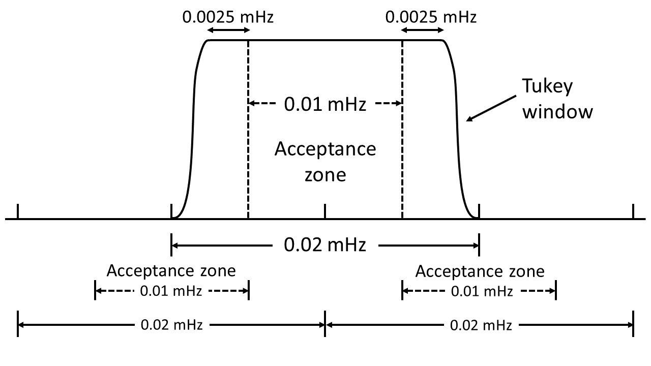
Figure 3: Schematic diagram of the windowing scheme. In this example, a Tukey window bandlimits the data in the Fourier domain to $0.02$ mHz. Only the estimated sources that belong to the central $0.01$ mHz interval, called the acceptance zone, are retained as identified sources. The acceptance zone is narrower than the flat part of the Tukey window that covers $75\%$ of the full band. Adjacent $0.02$ mHz bands, having identical Tukey windows, are overlapped such that their acceptance zones are contiguous.

Fig. 4 illustrates the edge effect and its mitigation by overlapped Tukey windows. For a rectangular window and an acceptance zone spanning the whole band, the presence of a true source close to a band edge triggers a cluster of spurious sources as described earlier. The tapering of the Tukey window suppresses this effect substantially, thereby reducing the burden of dealing with spurious sources in subsequent stages of GBSIEVER.

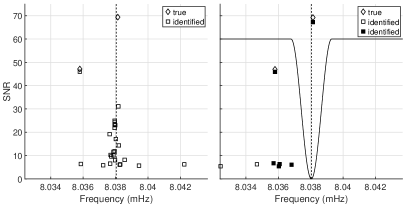
Figure 4: The edge effect and its mitigation with overlapped windowing. Each panel shows the halves of two adjacent non-overlapping bands, each $\approx 0.01$ mHz wide, along with their common edge (dashed line). The SNR and frequency of true (diamonds) and identified (squares) sources are shown for the case of (left panel) a rectangular window with an acceptance zone spanning the whole band, and (right panel) a Tukey window (solid line) with an acceptance zone that is narrower than its flat part. True sources that fall outside the acceptance zones of the bands shown here are recovered (filled squares) in the acceptance zone of the band (not shown) centered on the common edge.

IV.2 Undersampling and data length reduction

Computational efficiency in the calculation of the $\mathcal{F}$-statistic is of utmost importance in GBSIEVER since it must be evaluated a large number of times. This is achieved by evaluating all inner products (c.f., Eq. 16) using the method of undersampling [39] outlined below.

For a given band $[\nu,\nu+B]$, the DFT, $\widetilde{y}$, of the data is windowed as described in Sec. IV.1. The inverse DFT of the windowed data is then downsampled below the minimum Nyquist rate, $2(\nu+B)$, by retaining a regularly spaced subset of the samples. This direct sub-Nyquist rate sampling leads to aliasing error [40], but if the new sampling frequency is $f_{s}/d$, where $d$ is a positive integer such that $2(\nu+B)/n\leq f_{s}/d\leq 2\nu/(n-1)$ for an integer $n\in[1,(\nu+B)/B]$, its effect is to create a copy of the bandlimited spectrum in the baseband $[0,(f_{s}/d)/2]$. Thus, this clever use of aliasing error preserves the information in the original data while reducing the number of samples. Choosing the largest $n$ compatible with the bounds on $f_{s}/d$ yields the maximum allowed undersampling factor, $d$. As an example, for $\nu=5$ mHz, $B=0.02$ mHz, and $f_{s}=1/15$ Hz (the default sampling frequency of LDC1-4 data), undersampling reduces the number of samples by a factor $d=1414$. In contrast, if the data is simply downsampled to the minimum Nyquist rate, the reduction achieved is only a factor of $6$. The above procedure is followed for each band to generate the corresponding undersampled data vector that is then stored for subsequent processing.

The principal benefit of undersampling is the reduced computational cost of generating templates (c.f., Sec. III.1) on-the-fly in PSO since they need only be computed at the same time instants as the undersampled data. Since, unlike the data, templates are not explicitly bandlimited, the direct undersampling of a template incurs an error but it is negligible unless the frequency parameter, $f$, lies within $\Delta f_{\rm dplr}$ of a band edge. However, with a frequency this close to a band edge, the associated estimated source would be discarded anyway in the overlapped windowing scheme. Hence, for all practical purposes, the error in template waveforms due to undersampling is ignorable.

IV.3 Termination rule

The rule for terminating iterative source subtraction in a band can have a significant effect on the number and nature of identified sources. In GBSIEVER, termination happens when (i) a specified number, $N_{\rm term}$, of sources have been identified, or (ii) all the estimated source SNRs in $5$ consecutive iterations fall below a specified threshold $\eta_{\rm end}$. The second criterion accounts for the fact that identified sources are not found in a strictly descending order of SNR, especially as one approaches lower values, making termination based on a single instance of ${\rm SNR}<\eta_{\rm end}$ premature. Along the same lines, an identified source with ${\rm SNR}<\eta_{\rm end}$ is not discarded if it is an isolated case that is not in a chain of such SNRs. The second criterion leads to a substantial saving of computational cost provided it is reached first. Fortunately, this happens to be the case for LDC1-4 where the first criterion was used in only $21$ out of $1491$ bands.

IV.4 Cross-validation

A distinguishing feature of GBSIEVER is the mitigation of spurious sources by the cross-validation of identified ones. This is implemented by conducting two independent runs, called primary and secondary, of the iterative source estimation and subtraction in which the search ranges for $\dot{f}$ are set differently. The range used, denoted as $[\dot{f}_{\rm min},\dot{f}_{\rm max}]$, in the primary run is set such that $\dot{f}_{\rm min}<\dot{f}_{\rm min}^{(0)}$, $\dot{f}_{\rm max}>\dot{f}_{\rm max}^{(0)}$, where $\dot{f}_{\rm min}^{(0)}$ and $\dot{f}_{\rm max}^{(0)}>f_{\rm min}^{(0)}$ bound the astrophysically plausible range of $\dot{f}$. Once the range is set for the primary run, the only requirement on the $\dot{f}$ range in the secondary run is that it should be substantially different.

Next, for the set of estimated parameters $\Theta_{a}=\{\widehat{\theta}_{a,j}\}$, $j=1,\ldots,M_{a}$, of identified sources from the primary ($a=1$) and secondary ($a=2$) runs, we compute,

$$R_{\rm ee}(\widehat{\theta}_{1,i}) =\max_{j}R(\widehat{\theta}_{1,i},\widehat{\theta}_{2,j})\;.$$ (20)

A high value of $R_{\rm ee}$ indicates that an identified source is a genuine source since it appears in both of the independent searches with similar signal waveforms, while a low value indicates the contrary. Thus, an identified source from the primary run is admitted into the set of reported sources only if its $R_{\rm ee}$ value exceeds a specified threshold. As shown by our results in Sec. V.3, and Fig. 6 in particular, the use of cross-validation as defined above is highly effective in weeding out spurious sources.

V Results

In this section we describe the settings for GBSIEVER, the metrics used for assessing its performance, the results obtained, and the computational costs associated with the current code.

V.1 Settings

The user-specified settings for GBSIEVER and their values for the runs on LDC1-4 and MLDC-3.1mod are listed below.

• Width of search bands: While a bandwidth $B_{i}$ that adapts to the local density of sources is preferable for the GB resolution problem, the current version of GBSIEVER keeps $B_{i}=B$, a constant, for the sake of a simpler code. We set $B=0.02$ mHz and the starting frequency of the first band at $0.09$ mHz. The former is primarily based on considerations of parallelization on the computing clusters that were used, while the latter is the minimum source frequency in LDC1-4.

• Termination settings: As per the description of the termination criterion in Sec. IV.3, we set $N_{\rm term}=200$ and $\eta_{\rm end}\simeq 7$ [41] for all the bands. These settings were determined empirically, along with the number of search bands above, to keep the computational cost of the whole search within reasonable bounds.

• Edge effect mitigation: The flat part of the Tukey window used for bandlimiting the DFT of the data is $0.015$ mHz wide and the acceptance zone is set to $0.01$ mHz.

• Cross-validation: As mentioned in Sec. IV.4, the search range for $\dot{f}$ in the primary run should be guided by astrophysical expectations. In this paper, we follow the simpler option of using the known $\dot{f}$ ranges given in Sec. II to set the ranges as $[-10^{-16},10^{-15}]$ ${\rm Hz}^{2}$ and $[-10^{-14},10^{-13}]$ ${\rm Hz}^{2}$ for $f\leq 4$ mHz and $f\in[4,15]$ mHz, respectively. The secondary run is used in this paper only for sources below $4$ mHz because it reduces computational costs while preserving the impact of cross-validation where it matters the most. For the principal results, the secondary run $\dot{f}$ range is set at $[-10^{-14},10^{-13}]$ ${\rm Hz}^{2}$. However, we have also explored the efficacy of other combinations of primary and secondary search ranges in cross-validation as described later.

• SNR and $R_{ee}$ cuts: The set of reported sources is extracted from the set of identified ones based on their estimated SNR and $R_{ee}$. We consider several combinations of these cuts as discussed in Sec. V.3.

The search ranges for $\lambda$ and $\beta$ cover the whole sky: $\lambda\in[0,2\pi]$ and $\beta\in[-\pi/2,\pi/2]$. The settings for PSO have already been described in Sec. III.4. Elaborating on the $\dot{f}$ ranges for the primary run, we note that $\simeq 99.99\%$ of LDC1-4 sources with $f<4$ mHz have $\dot{f}$ values in $\simeq[-7.2\times 10^{-18},6.2\times 10^{-17}]$ ${\rm Hz}^{2}$, while $\gtrsim 99.9\%$ of them have $\dot{f}$ values in $\simeq[-3.0\times 10^{-15},2.4\times 10^{-14}]$ ${\rm Hz}^{2}$ for $f\in[4,15]$ mHz. The corresponding numbers for MLDC-3.1 are substantially similar. Thus, the $\dot{f}$ ranges for the primary run are actually much wider than the respective ranges for the vast majority of true sources.

V.2 Performance metrics

As indicated earlier, the standard metric [20] used to judge the performance of a GB resolution method is the detection rate: this is the fraction of reported sources that pass a test of association with true sources. The test used in this paper follows the one in MLDC-3 [21] and is defined below.

For each reported source, $\widehat{\theta}$, the true source $\theta$ is found which (a) has an ${\rm SNR}\geq 3$, (b) has a frequency within $6$ DFT frequencies of $\widehat{f}$, and (c) has the lowest distance, defined as $\sum_{I}(\|\overline{s}(\widehat{\theta})-\overline{s}(\theta)\|^{I})^{2}$, from the reported source. A reported source is confirmed if $R(\theta,\widehat{\theta})\geq 0.9$.

There are variations of the above test in the literature. In [25], the cutoff value for the ${\rm SNR}$ is $\gtrsim 1$ and no mention is made of a requirement on frequency difference. In [26], the SNR criteria is implemented by restricting the true sources to the brightest $\approx 40,000$, the frequency separation is reduced to $1$ DFT frequency, and the minimization of distance is replaced by the maximization of $R(\theta,\widehat{\theta})$.

It can happen occasionally that the same true source becomes the best match, in terms of the $R(\theta,\widehat{\theta})$ value, for multiple reported sources. This wrinkle in assessing GB resolution was identified in [26] and handled by confirming only the source with the highest $R$ (which may be $<0.9$) from such an ambiguous set. We apply the same remedy but only for reported sources in the ambiguous set that have $R(\theta,\widehat{\theta})\geq 0.9$ for the same true source – if this threshold is not crossed, none of the reported sources in the ambiguous set are confirmed. While this reduces the number of confirmed sources, the count of reported sources is not touched, thereby resulting in a conservative estimate of the detection rate. In practice, we found this to be a negligible issue: for example, in one set of $\approx 12,000$ reported sources only a single true source, matching a pair of reported sources with $R(\theta,\widehat{\theta})>0.9$, was found.

For assessing the parameter estimation performance of GBSIEVER, we follow the convention common to past challenges and consider only the mismatch of parameters between pairs of confirmed and true sources.

V.3 Source resolution performance

The extraction of reported sources from the set of identified ones is governed by SNR and $R_{\rm ee}$ cuts (c.f., Sec. IV.4). We have the freedom to impose different SNR cuts in different frequency intervals, as well as different $R_{\rm ee}$ cuts for identified sources above and below a given SNR threshold. The latter is guided by the expectation that the fraction of spurious sources should increase as one goes lower in SNR and, hence, the $R_{\rm ee}$ cutoff to weed them out must be set higher. Fig. 5 provides a schematic diagram of how the SNR and $R_{\rm ee}$ cuts are implemented: the SNR-frequency plane is partitioned into rectangular blocks and each block has an associated $R_{\rm ee}$ cutoff that is applied to the identified sources in that block.

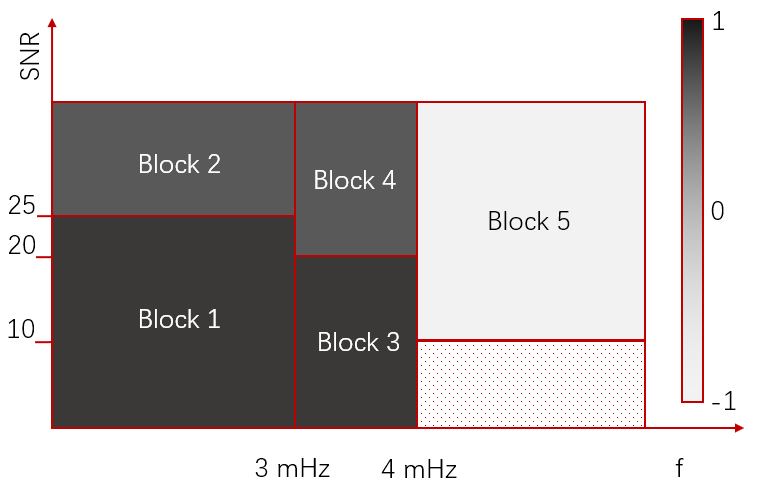
Figure 5: Schematic diagram of the cuts used for extracting reported sources from identified ones. The SNR-frequency plane is partitioned into blocks and an identified source falling into a given block is subjected to an $R_{\rm ee}$ threshold indicated by the shading of the block: the correspondence between the shading and the numerical value of $R_{\rm ee}$ is shown in the bar at right. The boundaries defining the blocks in this figure are for illustration only. (Note an $R_{\rm ee}$ cut is actually not used in this paper for $f\geq 4$ mHz.)

Each combination of SNR and $R_{\rm ee}$ cuts in a given frequency interval provides a different trade off between the detection rate and the search depth – the minimum SNR found for confirmed sources – for that interval. Thus, by slicing and dicing the same set of identified sources with different combinations of cuts, we can generate sets of reported sources that are tailored for specific science goals. In some cases, such as electromagnetic follow ups, one may want this set to have as low a contamination from spurious sources as possible in order to reduce wasted telescope time. In others, such as the estimation of the GB population distribution, completeness of the reported sample in terms of SNR may be an important consideration while the tolerance to spurious sources could be higher.

To determine the suitability of a given combination of frequency intervals and their corresponding SNR and $R_{\rm ee}$ cuts, robust estimates of the expected search depths and detection rates as well as their associated uncertainties would be required. These can be obtained from an ensemble of mock data realizations drawn from a range of realistic astrophysical models. While such an exhaustive analysis is outside the scope of this paper, it motivates a preliminary exploration of the effect of different combinations of cuts using the two mock data realizations we have in hand.

Table 1 presents the results for several different combinations of SNR and $R_{\rm ee}$ cuts for LDC1-4. The corresponding results for MLDC-3.1mod are given in Table 2. The combinations of cuts are labeled as follows and they are identical across LDC1-4 and MLDC-3.1mod.

• $R_{\rm ee}$–OFF: No $R_{\rm ee}$ cut used and the only cut applied is on SNR. Hence, cross-validation is not used at all in filtering out reported sources from the set of identified ones.

• $R_{\rm ee}$–ON: The same SNR cuts as in $R_{\rm ee}$–OFF but $R_{\rm ee}$ cuts are initiated in two out of the 4 blocks below $4$ mHz.

• SNR–UP: Same as $R_{\rm ee}$–ON but $R_{\rm ee}$ cuts are applied to all the blocks below $4$ mHz.

• SNR–DOWN: Same $R_{\rm ee}$ cuts as in SNR–UP but the SNR cut in each block is lower.

• MAIN: A combination of higher SNR but lower $R_{\rm ee}$ cuts relative to SNR–UP that provides our principal reported results.

In these tables, since $R_{\rm ee}\in[-1,1]$ by definition, $R_{\rm ee}=-1$ for a block indicates that no $R_{\rm ee}$ cutoff was applied while $R_{\rm ee}=1$ implies that all identified sources were rejected. The choice of frequency intervals, while being adjustable in principle, is kept the same in this paper for all of the above combinations.

Comparing $R_{\rm ee}$–OFF and $R_{\rm ee}$–ON in Table 1, we see how cross-validation improves the detection rate. The improvement is modest because the $R_{\rm ee}$ cut is used only in blocks $2$ and $4$, where the identified source SNRs are already high and, hence, the contamination from spurious sources is low. The importance of cross-validation becomes apparent when the $R_{\rm ee}$ cut is extended to blocks $1$ and $3$ in SNR–UP: we get $1,468$ and $981$ additional reported and confirmed sources, respectively. Lowering the SNR cuts in each block yields more confirmed sources in SNR–DOWN albeit with a slightly reduced detection rate.

Finally, for MAIN, comprised of higher SNR cuts (relative to SNR–UP) and lower $R_{\rm ee}$ cuts, GBSIEVER recovers $10,341$ confirmed sources in LDC1-4 – the largest among all the combinations – with an overall detection rate of $84.28\%$. While the search depth for the $[3,4]$ mHz band in MAIN is the same as that for SNR–UP/DOWN, it improves significantly, from $9.0$ to $7.5$, at frequencies below $3$ mHz. As seen for the $R_{\rm ee}$–ON combination, it is possible to reach an overall detection rate of $\gtrsim 90\%$ if identified sources in blocks 1 and 3 are discarded. While this reduces the total number of confirmed sources, $\approx 8,500$ were still recovered across the $[0,15]$ mHz band.

The results for MLDC-3.1mod can be analyzed in a similar fashion as above. Here, we simply highlight the fact that both the total number of confirmed sources, $10,136$, as well as the overall detection rate, $84.16\%$, for MAIN in Table 2 are similar to those for LDC1-4. This is not surprising even though MLDC-3.1mod has a much larger number of GBs because, as shown in Fig. 2, most of the excess sources have low amplitudes and, hence, are not resolvable.

The effectiveness of cross-validation in improving the quality of reported sources is demonstrated in Fig. 6. Not having an $R_{\rm ee}$ cut leads to a large excess of reported sources that have low correlations with true sources: following the discussion in Sec. V.2, these are more likely to be spurious sources. The effectiveness of the $R_{\rm ee}$ cut is most striking for the frequency interval below $3$ mHz, where source confusion is at its highest. While there is some loss of confirmed sources due to the $R_{\rm ee}$ cut, the much larger reduction in spurious sources boosts the detection rate significantly.

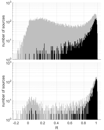
Figure 6: Histograms of the correlation coefficient between reported and true sources (c.f., Sec. V.2) with and without cross-validation. The top and bottom panels correspond to blocks $1$ and $3$, respectively, for the combination of cuts called MAIN in Table 1. The darker shaded histograms correspond to the reported sources as obtained with the cuts for these blocks while the lighter shaded ones correspond to reported sources for these blocks with the $R_{\rm ee}$ cut removed. Without the $R_{\rm ee}$ cut, the detection rates for blocks 1 and 3 fall from their values given in Table 1 to $17.51\%$ and $57.26\%$, respectively. The $R_{\rm ee}$ cut is seen to predominantly affect the reported sources having low correlations that are also more likely to be spurious.

The above remarks relate to the SNR and $R_{\rm ee}$ cuts within the framework of a cross-validation scheme that used a much wider secondary $\dot{f}$ search range than the primary one. Table. 3 contains results from an exploration of alternative schemes. In one, the secondary $\dot{f}$ range is reduced by a factor of $10$ with no change to the primary. In the other, the secondary range is brought down to a fixed value, $\dot{f}=0$, while the primary range is expanded by a factor of $100$. The SNR and $R_{\rm ee}$ cuts are the same in both the cases and identical to those for the SNR–UP combination in Table. 1.

We see that reducing the secondary range by a factor of $10$ increases the total number of confirmed sources to $\approx 11,000$ but worsens the detection rate. This is most notable in block 1, where it falls from $59.69\%$ (c.f., SNR–UP in Table. 1) to $48.05\%$. Remarkably, removing $\dot{f}$ as a search parameter altogether in the secondary run does not invalidate the effectiveness of cross-validation. In fact, it significantly improves the detection rate in block 1 but incurs a reduced number of confirmed sources and worsening of the search depth.

Our results indicate that it may be possible in a future version of GBSIEVER to refine the cross-validation scheme further by using a mix of secondary runs, with different search ranges for $\dot{f}$ adapted to different frequency ranges.

A final remark here is on the role of the assumed noise PSD in source resolution performance. In this paper, the noise PSD in the definition of SNR is that of the instrumental noise. This means that an identified source with SNR near the termination threshold (Sec. IV.3) is not strong relative to the dominant noise, namely confusion, at low frequencies. A uniform SNR termination threshold for all frequency bands leads, therefore, to more spurious identified sources at lower frequencies. However, the final set of reported sources is determined by the SNR and $R_{\rm ee}$ cuts, which are independent of the termination threshold, and these can be adjusted to account for higher noise where needed. (There is a degeneracy between the value used for an SNR cut and the choice of the PSD used in its definition – either one or both can be tuned for extracting reported sources.)

$R_{\rm ee}$–OFF	Block 1		Block 2		Block 3		Block 4		Block 5
	$\nu$ mHz	SNR	$\nu$ mHz	SNR	$\nu$ mHz	SNR	$\nu$ mHz	SNR	$\nu$ mHz	SNR
	$[0,3]$	$[0,20]$	$[0,3]$	$[20,\infty]$	$[3,4]$	$[0,15]$	$[3,4]$	$[15,\infty]$	$[4,15]$	$[10,\infty]$
$R_{\rm ee}$	$1$		$-1$		$1$		$-1$		$-1$
Identified	$20397$		$3254$		$2741$		$2314$		$4281$
Reported	$0$		$3254$		$0$		$2314$		$4281$
Detection rate	$0\%$		$83.53\%$		$0\%$		$87.51\%$		$94.23\%$
Lowest SNR (confirmed)	$20.0$				$15.0$				$10.0$
Total reported	$9849$
Total confirmed	$8777$
Detection rate	$89.12\%$
$R_{\rm ee}$–ON	Block 1		Block 2		Block 3		Block 4		Block 5
	$\nu$ mHz	SNR	$\nu$ mHz	SNR	$\nu$ mHz	SNR	$\nu$ mHz	SNR	$\nu$ mHz	SNR
	$[0,3]$	$[0,20]$	$[0,3]$	$[20,\infty]$	$[3,4]$	$[0,15]$	$[3,4]$	$[15,\infty]$	$[4,15]$	$[10,\infty]$
$R_{\rm ee}$	$1$		$0.9$		$1$		$0.9$		$-1$
Identified	$20397$		$3254$		$2741$		$2314$		$4281$
Reported	$0$		$2886$		$0$		$2124$		$4281$
Detection rate	$0\%$		$87.21\%$		$0\%$		$90.44\%$		$94.23\%$
Lowest SNR (confirmed)	$20.0$				$15.0$				$10.0$
Total reported	$9291$
Total confirmed	$8472$
Detection rate	$91.19\%$
SNR–UP	Block 1		Block 2		Block 3		Block 4		Block 5
	$\nu$ mHz	SNR	$\nu$ mHz	SNR	$\nu$ mHz	SNR	$\nu$ mHz	SNR	$\nu$ mHz	SNR
	$[0,3]$	$[0,20]$	$[0,3]$	$[20,\infty]$	$[3,4]$	$[0,15]$	$[3,4]$	$[15,\infty]$	$[4,15]$	$[10,\infty]$
$R_{\rm ee}$	$0.99$		$0.9$		$0.99$		$0.9$		$-1$
Identified	$20397$		$3254$		$2741$		$2314$		$4281$
Reported	$918$		$2886$		$550$		$2124$		$4281$
Detection rate	$59.69\%$		$87.21\%$		$78.73\%$		$90.44\%$		$94.23\%$
Lowest SNR (confirmed)	$9.0$				$6.6$				$10.0$
Total reported	$10759$
Total confirmed	$9453$
Detection rate	$87.86\%$
SNR–DOWN	Block 1		Block 2		Block 3		Block 4		Block 5
	$\nu$ mHz	SNR	$\nu$ mHz	SNR	$\nu$ mHz	SNR	$\nu$ mHz	SNR	$\nu$ mHz	SNR
	$[0,3]$	$[0,15]$	$[0,3]$	$[15,\infty]$	$[3,4]$	$[0,10]$	$[3,4]$	$[10,\infty]$	$[4,15]$	$[8,\infty]$
$R_{\rm ee}$	$0.99$		$0.9$		$0.99$		$0.9$		$-1$
Identified	$18001$		$5650$		$1462$		$3593$		$4550$
Reported	$258$		$4016$		$99$		$2874$		$4550$
Detection rate	$51.16\%$		$80.13\%$		$63.64\%$		$87.72\%$		$90.55\%$
Lowest SNR (confirmed)	$9.0$				$6.6$				$8.0$
Total reported	$11797$
Total confirmed	$10054$
Detection rate	$85.23\%$
MAIN	Block 1		Block 2		Block 3		Block 4		Block 5
	$\nu$ mHz	SNR	$\nu$ mHz	SNR	$\nu$ mHz	SNR	$\nu$ mHz	SNR	$\nu$ mHz	SNR
	$[0,3]$	$[0,25]$	$[0,3]$	$[25,\infty]$	$[3,4]$	$[0,20]$	$[3,4]$	$[20,\infty]$	$[4,15]$	$[10,\infty]$
$R_{\rm ee}$	$0.9$		$0.5$		$0.9$		$0.5$		$-1$
Identified	$21546$		$2105$		$3531$		$1524$		$4281$
Reported	$2778$		$2072$		$1629$		$1510$		$4281$
Detection rate	$62.56\%$		$91.17\%$		$79.13\%$		$92.12\%$		$94.23\%$
Lowest SNR (confirmed)	$7.5$				$6.6$				$10.0$
Total reported	$12270$
Total confirmed	$10341$
Detection rate	$84.28\%$

Table 1: Performance of GBSIEVER for different combinations of SNR and $R_{\rm ee}$ cuts on LDC1-4 data. For cross-validation (implemented for $f\leq 4$ mHz), the primary and secondary search ranges for $\dot{f}$ are $[-10^{-16},10^{-15}]~{}\rm{Hz^{2}}$ and $[-10^{-14},10^{-13}]~{}\rm{Hz^{2}}$ respectively. A block for which the $R_{\rm ee}$ cut was not used is shown as having $R_{\rm ee}=-1$, while $R_{\rm ee}=1$ means that the identified sources in that block were discarded.

$R_{\rm ee}$–OFF	Block 1		Block 2		Block 3		Block 4		Block 5
	$\nu$ mHz	SNR	$\nu$ mHz	SNR	$\nu$ mHz	SNR	$\nu$ mHz	SNR	$\nu$ mHz	SNR
	$[0,3]$	$[0,20]$	$[0,3]$	$[20,\infty]$	$[3,4]$	$[0,15]$	$[3,4]$	$[15,\infty]$	$[4,15]$	$[10,\infty]$
$R_{\rm ee}$	$1$		$-1$		$1$		$-1$		$-1$
Identified	$20914$		$3253$		$3412$		$2204$		$4582$
Reported	$0$		$3253$		$0$		$2204$		$4582$
Detection rate	$0\%$		$84.69\%$		$0\%$		$86.21\%$		$91.58\%$
Lowest SNR (confirmed)	$20.0$				$15.0$				$10.0$
Total reported	$10039$
Total confirmed	$8851$
Detection rate	$88.17\%$
$R_{\rm ee}$–ON	Block 1		Block 2		Block 3		Block 4		Block 5
	$\nu$ mHz	SNR	$\nu$ mHz	SNR	$\nu$ mHz	SNR	$\nu$ mHz	SNR	$\nu$ mHz	SNR
	$[0,3]$	$[0,20]$	$[0,3]$	$[20,\infty]$	$[3,4]$	$[0,15]$	$[3,4]$	$[15,\infty]$	$[4,15]$	$[10,\infty]$
$R_{\rm ee}$	$1$		$0.9$		$1$		$0.9$		$-1$
Identified	$20914$		$3253$		$3412$		$2204$		$4582$
Reported	$0$		$2868$		$0$		$1937$		$4582$
Detection rate	$0\%$		$88.18\%$		$0\%$		$90.24\%$		$91.58\%$
Lowest SNR (confirmed)	$20.0$				$15.0$				$10.0$
Total reported	$9387$
Total confirmed	$8473$
Detection rate	$90.26\%$
SNR–UP	Block 1		Block 2		Block 3		Block 4		Block 5
	$\nu$ mHz	SNR	$\nu$ mHz	SNR	$\nu$ mHz	SNR	$\nu$ mHz	SNR	$\nu$ mHz	SNR
	$[0,3]$	$[0,20]$	$[0,3]$	$[20,\infty]$	$[3,4]$	$[0,15]$	$[3,4]$	$[15,\infty]$	$[4,15]$	$[10,\infty]$
$R_{\rm ee}$	$0.99$		$0.9$		$0.99$		$0.9$		$-1$
Identified	$20914$		$3253$		$3412$		$2204$		$4582$
Reported	$797$		$2868$		$427$		$1937$		$4582$
Detection rate	$62.99\%$		$88.18\%$		$74.00\%$		$90.24\%$		$91.58\%$
Lowest SNR (confirmed)	$7.8$				$7.7$				$10.0$
Total reported	$10611$
Total confirmed	$9291$
Detection rate	$87.56\%$
SNR–DOWN	Block 1		Block 2		Block 3		Block 4		Block 5
	$\nu$ mHz	SNR	$\nu$ mHz	SNR	$\nu$ mHz	SNR	$\nu$ mHz	SNR	$\nu$ mHz	SNR
	$[0,3]$	$[0,15]$	$[0,3]$	$[15,\infty]$	$[3,4]$	$[0,10]$	$[3,4]$	$[10,\infty]$	$[4,15]$	$[8,\infty]$
$R_{\rm ee}$	$0.99$		$0.9$		$0.99$		$0.9$		$-1$
Identified	$18499$		$5668$		$1874$		$3742$		$5055$
Reported	$202$		$3977$		$57$		$2631$		$5055$
Detection rate	$51.98\%$		$80.94\%$		$61.40\%$		$86.66\%$		$85.68\%$
Lowest SNR (confirmed)	$7.8$				$7.7$				$8.0$
Total reported	$11922$
Total confirmed	$9970$
Detection rate	$83.63\%$
MAIN	Block 1		Block 2		Block 3		Block 4		Block 5
	$\nu$ mHz	SNR	$\nu$ mHz	SNR	$\nu$ mHz	SNR	$\nu$ mHz	SNR	$\nu$ mHz	SNR
	$[0,3]$	$[0,25]$	$[0,3]$	$[25,\infty]$	$[3,4]$	$[0,20]$	$[3,4]$	$[20,\infty]$	$[4,15]$	$[10,\infty]$
$R_{\rm ee}$	$0.9$		$0.5$		$0.9$		$0.5$		$-1$
Identified	$22054$		$2113$		$4223$		$1393$		$4582$
Reported	$2553$		$2096$		$1443$		$1370$		$4582$
Detection rate	$62.48\%$		$92.56\%$		$78.79\%$		$92.55\%$		$91.58\%$
Lowest SNR (confirmed)	$7.8$				$7.7$				$10.0$
Total reported	$12044$
Total confirmed	$10136$
Detection rate	$84.16\%$

Table 2: Performance of GBSIEVER for different combinations of SNR and $R_{\rm ee}$ cuts on MLDC-3.1mod data. For cross-validation (implemented for $f\leq 4$ mHz), the primary and secondary search ranges for $\dot{f}$ are $[-10^{-16},10^{-15}]~{}\rm{Hz^{2}}$ and $[-10^{-14},10^{-13}]~{}\rm{Hz^{2}}$ respectively. A block for which the $R_{\rm ee}$ cut was not used is shown as having $R_{\rm ee}=-1$, while $R_{\rm ee}=1$ means that the identified sources in that block were discarded.

$\begin{array}[]{lr}{\rm primary:}&[-10^{-16},10^{-15}]~{}\rm{Hz^{2}}\\ {\rm secondary:}&[-10^{-15},10^{-14}]~{}\rm{Hz^{2}}\end{array}$	Block 1		Block 2		Block 3		Block 4		Block 5
	$\nu$ mHz	SNR	$\nu$ mHz	SNR	$\nu$ mHz	SNR	$\nu$ mHz	SNR	$\nu$ mHz	SNR
	$[0,3]$	$[0,20]$	$[0,3]$	$[20,\infty]$	$[3,4]$	$[0,15]$	$[3,4]$	$[15,\infty]$	$[4,15]$	$[10,\infty]$
$R_{\rm ee}$	$0.99$		$0.9$		$0.99$		$0.9$		$-1$
Identified	$20397$		$3254$		$2741$		$2314$		$4281$
Reported	$3003$		$3114$		$1198$		$2235$		$4281$
Detection rate	$48.05\%$		$85.36\%$		$71.87\%$		$89.08\%$		$94.23\%$
Lowest SNR (confirmed)	$7.2$				$7.0$				$10.0$
Total reported	$13831$
Total confirmed	$10987$
Detection rate	$79.44\%$
$\begin{array}[]{lr}{\rm primary:}&[-10^{-14},10^{-13}]~{}\rm{Hz^{2}}\\ {\rm secondary:}&[0,0]~{}\rm{Hz^{2}}\end{array}$	Block 1		Block 2		Block 3		Block 4		Block 5
	$\nu$ mHz	SNR	$\nu$ mHz	SNR	$\nu$ mHz	SNR	$\nu$ mHz	SNR	$\nu$ mHz	SNR
	$[0,3]$	$[0,20]$	$[0,3]$	$[20,\infty]$	$[3,4]$	$[0,15]$	$[3,4]$	$[15,\infty]$	$[4,15]$	$[10,\infty]$
$R_{\rm ee}$	$0.99$		$0.9$		$0.99$		$0.9$		$-1$
Identified	$22149$		$3147$		$3021$		$2284$		$4281$
Reported	$570$		$2752$		$328$		$2037$		$4281$
Detection rate	$71.58\%$		$87.72\%$		$86.28\%$		$91.65\%$		$94.23\%$
Lowest SNR (confirmed)	$9.0$				$6.9$				$10.0$
Total reported	$9968$
Total confirmed	$9006$
Detection rate	$90.35\%$

Table 3: Performance of GBSIEVER for the same combination of SNR and $R_{\rm ee}$ cuts on LDC1-4 data but different choices for $\dot{f}$ search ranges in the primary and secondary runs as listed in the heading for each combination. A block for which the $R_{\rm ee}$ cut was not used is shown as having $R_{\rm ee}=-1$.

V.4 Residuals

Resolving GBs is not only important in and of itself but also crucial to the extraction of other types of sources from LISA data. This calls for an examination of the residual data in a TDI combination after subtracting out the signals of reported GBs. We do this only for LDC1-4 TDI A and the reported sources obtained with the combination of SNR and $R_{\rm ee}$ cuts called MAIN in Table 1. The results for TDI E and other combinations of cuts are visually indistinguishable from the ones shown here.

Figure 7 compares the periodogram (magnitude of the DFT) and PSD of the residual with those of the data and the instrumental noise realization in the data. We see that the PSD of the residual is brought down to the level of the instrumental noise for frequencies $\gtrsim 4$ mHz. In fact, the cross-correlation coefficient between the residual and instrumental noise time series, both bandlimited to $[4,15]$ mHz, is $0.9973$, indicating that they are nearly identical and that practically all resolvable GBs were removed with high accuracy.

It is worth emphasizing here the necessity of comparing the residual with the instrumental noise and not just the data. This is illustrated in Fig. 8, where the residuals after subtracting the reported and identified sources in the $[4,15]$ mHz range are compared. We see that the PSD of the residual corresponding to the latter set, which has more spurious sources by definition, now lies below that of the instrumental noise. This is clearly an artifact of overfitting that comparing the PSDs of the residual and data alone would not reveal, misleading one into thinking that the GBs had been subtracted out faithfully.

Starting below $4$ mHz, the residual power increases towards lower frequencies due to the rising confusion between the ever more crowded signals. It is interesting to note in Fig. 7 that the PSD of the residual is less spiky compared to that of the data. This is an indication that loud resolvable sources have been taken out successfully.

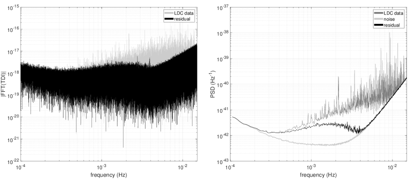
Figure 7: Periodogram (left) and PSD (right) of the residual after removing the reported sources for the MAIN combination in Table 1 from LDC1-4 TDI A data. The frequency resolution of the PSD is $8.1380\times 10^{-3}$ mHz.

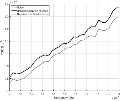
Figure 8: PSD of the residual in the $[4,15]$ mHz range obtained by removing (black curve) only the reported sources in the MAIN combination of Table 1, and (gray curve) all the identified sources. Due to a higher fraction of spurious sources in the latter set, the residual PSD is lowered below that of the instrumental noise (dotted curve). (The displayed frequency interval has been restricted to $[7,8]$ mHz for visual clarity.)

V.5 Parameter estimation performance

Figures 9 and 10 show the marginal distributions of the differences between the parameters of confirmed and true sources. They appear to be qualitatively similar to those in [26, 25].

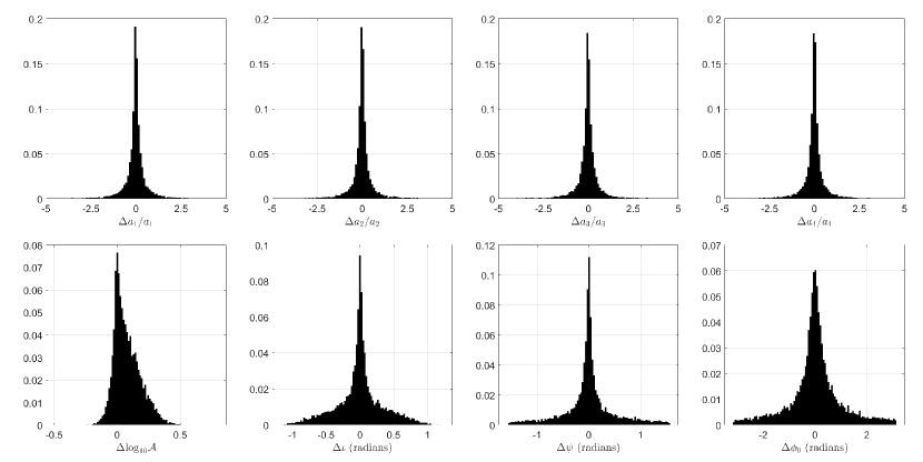
Figure 9: Histogram of the differences between the extrinsic parameters of confirmed and true sources in LDC1-4 data. The confirmed sources are obtained from the combination of cuts called MAIN in Table 1. For each distribution, a small fraction of outliers are not shown for visual clarity. The number of outliers dropped, as a fraction of the $10,341$ confirmed sources, for $\Delta a_{i}$, $i=1$ to $4$, are $2.6\%$, $2.4\%$, $2.6\%$, and $2.7\%$, respectively. Note that the extrinsic parameters in the bottom row are functions of the ones in the top row.

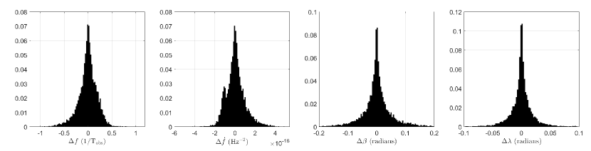
Figure 10: Histogram of the differences between the intrinsic parameters of confirmed and true sources in LDC1-4 data. The confirmed sources are obtained from the combination of cuts called MAIN in Table 1. In the distributions of $\Delta\beta$ and $\Delta\lambda$, $1.5\%$ and $1\%$, respectively, of the $10,341$ confirmed sources have been dropped for visual clarity.

It is worth noting that the differences in parameter values are computed over a spread in true source parameters and their distributions are, in general, not the same as those of parameter estimation errors for a fixed true source. (The former are mixture distributions while the latter are not.) In particular, the distribution of parameter differences will be affected by the distribution of the SNR of resolvable sources. This is illustrated in Fig. 11 containing scatterplots of the differences against the true source SNR. It can be seen that the asymmetry in the distribution of $\Delta\log_{10}\mathcal{A}$ is more pronounced for lower SNR sources, which also happen to be predominantly at lower frequencies where the confusion between sources is higher. We conjecture that the higher density of sources at lower frequencies leads to spurious constructive interference that biases the estimation of the amplitude of a given source to higher values.

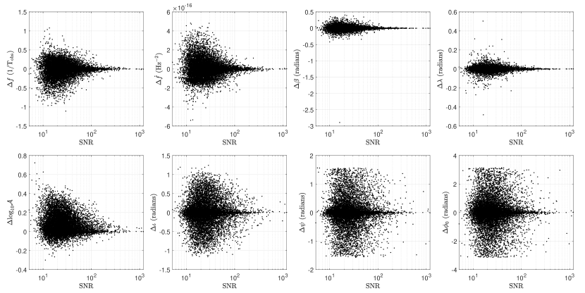
Figure 11: Scatterplots of differences in the parameters of confirmed and true sources in LDC1-4 against the SNR of the latter. The outliers that were excluded in Fig. 9 and Fig. 10 are included here.

Overall, the estimation of every parameter shows asymptotic convergence to the true parameter with increasing SNR. This supports the statistical consistency of the iterative source subtraction approach to GB resolution.

V.6 Computational considerations

Cross-validation requires at least two complete passes of a multi-source resolution method on the same data. Hence, its computational feasibility hinges on the runtime of the method. For GBSIEVER, the two main accelerators of runtime are the efficient global optimization of $\mathcal{F}$-statistic by PSO and the undersampling of template waveforms. The former reduces the number of $\mathcal{F}$-statistic evaluations while the latter speeds up each one.

The current implementation of GBSIEVER is in the Matlab [42] programming language. The $N_{\rm runs}$ independent PSO runs (c.f., Sec. III.4) are executed in parallel on a matching number of cores of a multi-core processor, while the frequency bands are analyzed in parallel on different nodes of a computing cluster. For each band and PSO run, the code completes the analysis of $2$ yr of data in $\lesssim 15$ hrs on a $2.3$ GHz core. A third level of parallelization, over PSO particle fitness evaluations in each iteration, is possible but this cannot be implemented in Matlab and requires a compiled language such as C. In principle, achieving all three layers of parallelization could speed up the code by up to a factor of $\lesssim 40$, the number of PSO particles. (The shift to a compiled language by itself should afford a significant increase in speed.)

VI Conclusions

We have presented a new method, GBSIEVER, for resolving Galactic binaries in LISA data and have quantified its performance on LDC1-4 and (modified) MLDC3.1 data. Our results affirm the validity of the iterative single source estimation and subtraction approach for the LISA multi-source resolution problem. The principal novel features of GBSIEVER are the use of PSO for maximization of the $\mathcal{F}$-statistic, fast template generation using undersampling, and mitigation of spurious sources using a cross-validation scheme. We also showed that the trade-off between the detection rate and the depth of the search can be tuned using different combinations of the cuts used for extracting reported sources from the initial set of identified ones.

Inspection of the residual left from the subtraction of reported sources shows that it is possible to reach the instrumental noise floor for frequencies $\gtrsim 4$ mHz. Increased confusion noise below $4$ mHz precludes this but the residual power still remains substantially lower than that of the data down to $\simeq 1$ mHz. We envision GBSIEVER to be a part of a hierarchical analysis pipeline where it will be applied to the residual after subtracting louder signals, such as massive black hole binaries, from the data. Provided such signals are reduced below the GB confusion noise, GBSIEVER can take over and find resolvable GBs. However, quantifying the effects of weaker non-GB sources left behind in the data on a pure GB search pipeline, such as GBSIEVER, remains an open question. The ability to reach the instrumental noise floor above $4$ mHz bodes well for the extraction of non-GB sources in this frequency band although an actual test must await future work.

The performance of GBSIEVER in terms of the number of reported sources, the detection rate, and differences between the parameters of confirmed and true sources is comparable to state-of-the-art methods. There remains substantial scope for improvements, ranging from minor, such as how PSO handles the search over the sky (currently treated as a box instead of a sphere), to major, such as supplementing iterative single source fitting with a global one that fits multiple sources simultaneously. The latter is also required to address a current limitation, namely, error estimates for the parameters of individual reported sources. Since the errors arise not only from instrumental or confusion noise but also from the presence of other resolvable sources, a global fit analysis is required. We also need to go beyond our current, empirically obtained, understanding of cross-validation and find out how to better control its performance.

With significantly improved runtimes in the future, it will become possible to characterize the performance of GBSIEVER on an ensemble of realizations of the GB population. This will, in turn, enable a statistically rigorous study of the effect of different combinations of cuts on detection rates and search depths.

References

- [1] J. Aasi et al., “Advanced LIGO,” Classical and quantum gravity, vol. 32, no. 7, p. 074001, 2015.
- [2] F. Acernese et al., “Advanced Virgo: a second-generation interferometric gravitational wave detector,” Classical and Quantum Gravity, vol. 32, no. 2, p. 024001, 2014.
- [3] B. Abbott et al., “GWTC-1: A Gravitational-Wave Transient Catalog of Compact Binary Mergers Observed by LIGO and Virgo during the First and Second Observing Runs,” Phys. Rev. X, vol. 9, no. 3, p. 031040, 2019.
- [4] R. Abbott et al., “GWTC-2: Compact Binary Coalescences Observed by LIGO and Virgo During the First Half of the Third Observing Run,” arXiv e-prints, p. arXiv:2010.14527, Oct. 2020.
- [5] T. Venumadhav, B. Zackay, J. Roulet, L. Dai, and M. Zaldarriaga, “New binary black hole mergers in the second observing run of Advanced LIGO and Advanced Virgo,” Phys. Rev. D, vol. 101, no. 8, p. 083030, 2020.
- [6] B. Abbott et al., “GW170817: Observation of Gravitational Waves from a Binary Neutron Star Inspiral,” Phys. Rev. Lett., vol. 119, no. 16, p. 161101, 2017.
- [7] P. Amaro-Seoane et al., “Laser Interferometer Space Antenna,” arXiv e-prints, p. arXiv:1702.00786, Feb. 2017.
- [8] M. Armano et al., “LISA Pathfinder: The experiment and the route to LISA,” Class. Quant. Grav., vol. 26, p. 094001, 2009.
- [9] W.-H. Ruan, Z.-K. Guo, R.-G. Cai, and Y.-Z. Zhang, “Taiji program: Gravitational-wave sources,” Int. J. Mod. Phys. A, vol. 35, no. 17, p. 2050075, 2020.
- [10] J. Luo et al., “TianQin: a space-borne gravitational wave detector,” Class. Quant. Grav., vol. 33, no. 3, p. 035010, 2016.
- [11] G. Hobbs, A. Archibald, Z. Arzoumanian, D. Backer, M. Bailes, N. Bhat, M. Burgay, S. Burke-Spolaor, D. Champion, I. Cognard, et al., “The international pulsar timing array project: using pulsars as a gravitational wave detector,” Classical and Quantum Gravity, vol. 27, no. 8, p. 084013, 2010.
- [12] Y. Wang and S. D. Mohanty, “Pulsar Timing Array Based Search for Supermassive Black Hole Binaries in the Square Kilometer Array Era,” Phys. Rev. Lett., vol. 118, no. 15, p. 151104, 2017. [Erratum: Phys.Rev.Lett. 124, 169901 (2020)].
- [13] G. Hobbs, S. Dai, R. N. Manchester, R. M. Shannon, M. Kerr, K. J. Lee, and R. Xu, “The Role of FAST in Pulsar Timing Arrays,” Res. Astron. Astrophys., vol. 19, no. 2, p. 020, 2019.
- [14] R. Smits, M. Kramer, B. Stappers, D. R. Lorimer, J. Cordes, and A. Faulkner, “Pulsar searches and timing with the square kilometre array,” Astron. Astrophys., vol. 493, pp. 1161–1170, 2009.
- [15] M. Tinto and S. V. Dhurandhar, “Time-Delay Interferometry,” Living Rev. Rel., vol. 17, p. 6, 2014.
- [16] M. L. Katz, L. Z. Kelley, F. Dosopoulou, S. Berry, L. Blecha, and S. L. Larson, “Probing Massive Black Hole Binary Populations with LISA,” Mon. Not. Roy. Astron. Soc., vol. 491, no. 2, pp. 2301–2317, 2020.
- [17] S. Babak, J. Gair, A. Sesana, E. Barausse, C. F. Sopuerta, C. P. Berry, E. Berti, P. Amaro-Seoane, A. Petiteau, and A. Klein, “Science with the space-based interferometer LISA. V: Extreme mass-ratio inspirals,” Phys. Rev. D, vol. 95, no. 10, p. 103012, 2017.
- [18] G. Nelemans, L. R. Yungelson, and S. F. Portegies Zwart, “The gravitational wave signal from the Galactic disk population of binaries containing two compact objects,” Astron. Astrophys., vol. 375, pp. 890–898, 2001.
- [19] K. A. Arnaud et al., “Report on the first round of the Mock LISA Data Challenges,” Classical and Quantum Gravity, vol. 24, no. 19, pp. S529–S539, 2007.
- [20] S. Babak et al., “Report on the second Mock LISA Data Challenge,” Class. Quant. Grav., vol. 25, p. 114037, 2008.
- [21] S. Babak et al., “The Mock LISA Data Challenges: from challenge 3 to challenge 4,” Classical and Quantum Gravity, vol. 27, no. 8, p. 084009, 2010.
- [22] LISA Consortium’s LDC working group, “(the new) LISA Data Challenges.” https://lisa-ldc.lal.in2p3.fr. Accessed: 2021-02-25.
- [23] S. D. Mohanty and R. K. Nayak, “Tomographic approach to resolving the distribution of LISA Galactic binaries,” Phys. Rev., vol. D73, p. 083006, 2006.
- [24] J. Crowder and N. J. Cornish, “Extracting Galactic binary signals from the first round of Mock LISA Data Challenges,” Classical and Quantum Gravity, vol. 24, pp. S575–S585, sep 2007.
- [25] T. B. Littenberg, “A detection pipeline for Galactic binaries in LISA data,” Phys. Rev., vol. D84, p. 063009, 2011.
- [26] A. Blaut, S. Babak, and A. Krolak, “Mock LISA Data Challenge for the Galactic white dwarf binaries,” Phys. Rev., vol. D81, p. 063008, 2010.
- [27] N. J. Cornish and S. L. Larson, “LISA data analysis: Source identification and subtraction,” Phys. Rev., vol. D67, p. 103001, 2003.
- [28] T. B. Littenberg, N. J. Cornish, K. Lackeos, and T. Robson, “Global analysis of the gravitational wave signal from galactic binaries,” Phys. Rev. D, vol. 101, p. 123021, 2020.
- [29] J. Kennedy and R. Eberhart, “Particle swarm optimization,” in Proceedings of ICNN’95-international conference on neural networks, vol. 4, pp. 1942–1948, IEEE, 1995.
- [30] A. Petiteau, G. Auger, H. Halloin, O. Jeannin, E. Plagnol, S. Pireaux, T. Regimbau, and J.-Y. Vinet, “LISACode: A Scientific simulator of LISA,” Phys. Rev., vol. D77, p. 023002, 2008.
- [31] N. J. Cornish and T. B. Littenberg, “Tests of bayesian model selection techniques for gravitational wave astronomy,” Phys. Rev. D, vol. 76, p. 083006, Oct 2007.
- [32] We could have used analytical formulae for but its direct estimation from the noise avoids problems arising from a mismatch of conventions.
- [33] A. P. Engelbrecht, Fundamentals of computational swarm intelligence, vol. 1. Wiley Chichester, 2005.
- [34] R. Eberhart and J. Kennedy, “A new optimizer using particle swarm theory,” in Micro Machine and Human Science, 1995. MHS’95., Proceedings of the Sixth International Symposium on, pp. 39–43, IEEE, 1995.
- [35] S. D. Mohanty, Swarm Intelligence Methods for Statistical Regression. Chapman and Hall/CRC, 2018.
- [36] D. Bratton and J. Kennedy, “Defining a standard for particle swarm optimization,” in 2007 IEEE Swarm Intelligence Symposium, pp. 120–127, 2007.
- [37] M. E. Normandin, S. D. Mohanty, and T. S. Weerathunga, “Particle swarm optimization based search for gravitational waves from compact binary coalescences: Performance improvements,” Physical Review D, vol. 98, no. 4, p. 044029, 2018.
- [38] J. Crowder and N. J. Cornish, “Solution to the Galactic foreground problem for LISA,” Phys. Rev. D, vol. 75, p. 043008, Feb 2007.
- [39] W. Kester, Mixed-signal and DSP design techniques. Newnes, 2003.
- [40] R. N. Bracewell, The Fourier transform and its applications. McGraw-Hill New York, 3 ed., 1986.
- [41] The threshold is actually based on the -statistic ( to be exact), hence the approximate value for SNR shown here.
- [42] The Mathworks, Inc., Natick, Massachusetts, MATLAB version 9.7.0.1261785 (R2019b), 2019.