Variability of Late-time Radio Emission in the Superluminous Supernova PTF10hgi

Abstract

We report the time variability of the late-time radio emission in a Type-I superluminous supernova (SLSN), PTF10hgi, at $z=0.0987$. The Karl G. Jansky Very Large Array 3-GHz observations at 8.6 and 10 years after the explosion both detected radio emission with a $\sim$40% decrease in flux density in the second epoch. This is the first report of a significant variability of the late-time radio light curve in a SLSN. Through combination with previous measurements in two other epochs, we constrained both the rise and decay phases of the radio light curve over three years, peaking at approximately 8–9 years after the explosion with a peak luminosity of $L_{\rm 3GHz}=2\times 10^{21}$ W Hz^-1. Possible scenarios for the origin of the variability are an active galactic nucleus (AGN) in the host galaxy, an afterglow caused by the interaction between an off-axis jet and circumstellar medium, and a wind nebula powered by a newly-born magnetar. Comparisons with models show that the radio light curve can be reproduced by both the afterglow model and magnetar wind nebula model. Considering the flat radio spectrum at 1–15 GHz and an upper limit at 0.6 GHz obtained in previous studies, plausible scenarios are a low-luminosity flat-spectrum AGN or a magnetar wind nebula with a shallow injection spectral index.

1 Introduction

Superluminous supernovae (SLSNe) are very bright explosions that are $\sim$10–100 times brighter than ordinary Type Ia and core-collapse supernovae (SNe) (see Gal-Yam, 2012, for a review). SLSNe are classified into two subclasses according to their spectra: hydrogen-poor SLSNe-I and hydrogen-rich SLSNe-II. Due to their huge luminosity and scarcity, the physical nature of SLSNe is still a matter of debate, and SLSNe-I are particularly among the least understood SN populations. There are many models proposed for progenitors and powering sources for SLSNe-I, such as pair-instability SNe (e.g., Woosley et al., 2007), spin-down of a newborn strongly magnetized neutron star (magnetar; e.g., Kasen & Bildsten, 2010), fallback accretion onto a compact remnant (Dexter & Kasen, 2013), and interaction a with dense circumstellar medium (CSM) (e.g., Chevalier & Irwin, 2011).

Late-time radio observations are useful to constrain the models of SLSNe. It is expected that radio emission arise from shock interaction between SN ejecta CSM. The connection between SLSNe-I and long-duration gamma-ray bursts (GRBs) has been suggested observationally and theoretically (e.g., Lunnan et al., 2014; Greiner et al., 2015; Metzger et al., 2015), and it is thought that an afterglow from an off-axis jet is observable in late-time at radio bands. Non-detections in previous studies constrained physical properties, such as energies, mass-loss rates, and CSM densities, for off-axis jets (e.g., Nicholl et al., 2016; Margalit et al., 2018; Coppejans et al., 2018). Based on the the model of a SN driven by a young pulsar or magnetar (Murase et al., 2016), Omand et al. (2018) predicted quasi-state synchrotron radio emission peaking at $\gtrsim$10 years after SN explosion, which can be tested with current radio telescopes. Radio observations by Hatsukade et al. (2018) put constraint on the predictions for one of the SLSNe by Omand et al. (2018).

Recently, Eftekhari et al. (2019) found an unresolved radio source coincident with the position of the SLSN-I SN 2010md/PTF10hgi. PTF10hgi was discovered on May 15, 2010 (Quimby et al., 2010) in a dwarf galaxy at $z=0.0987$ (Inserra et al., 2013; Lunnan et al., 2014; Leloudas et al., 2015). Spectral energy distribution (SED) analysis by Perley et al. (2016) and Schulze et al. (2018) obtained a star-formation rate (SFR) of $\sim$0.1–0.2 $M_{\odot}$ yr^-1 and stellar mass of $\log{M_{*}}=7.6$–7.9 $M_{\odot}$. Eftekhari et al. (2019) argued that the radio emission is consistent with an off-axis jet or wind nebula powered by a magnetar, suggesting the presence of a central engine. Further detections at 1.2, 3, and 15 GHz by Law et al. (2019) and Mondal et al. (2020) support the model of a magnetar-powered SLSN.

In this Letter, we report the time variability in the late-time radio emission of PTF10hgi based on our new 3-GHz radio continuum observations using the Karl G. Jansky Very Large Array (VLA). The remainder of the Letter is organized as follows. Section 2 describes the radio observations, and the results are presented in Section 3. In Section 4, we discuss the possible scenarios for the origin of the radio emission. Conclusions are presented in Section 5. Throughout the Letter, we adopt a Chabrier (2003) initial mass function and cosmological parameters based on the Planck 2018 results (Planck Collaboration et al., 2020). The luminosity distance to PTF10hgi is 469 Mpc, and $1^{\prime\prime}$ corresponds to 2.07 kpc.

2 VLA Observations

The VLA S-band 3-GHz (13-cm) observations were performed on December 2, 2018 in semester 18B (Project ID: 18B-077) and April 25, 2020 in semester 20A (Project ID: 20A-133) as part of a search for late-time radio emissions from SLSNe (B. Hatsukade et al., in preparation). The observation dates are 8.6 and 10 years after the discovery date of PTF10hgi, respectively. The observations were conducted in array configuration C with the baseline length ranging from 45 m to 3.4 km. The WIDAR correlator was used with 8-bit samplers. We used two basebands, each with a 1-GHz bandwidth, centered at 2.5 GHz and 3.5 GHz, which provided a total bandwidth of 2 GHz. The SN positions were used as phase centers of the observations. Bandpass and amplitude calibrations were conducted with 3C286, and phase calibrations were conducted with J1640+1220. The details are summarized in Table 1.

The data were reduced with Common Astronomy Software Applications (CASA; McMullin et al., 2007) release 5.6.2. The maps were produced with the task tclean. Briggs weighting with robust 0.5 was adopted. The absolute flux accuracy was estimated by comparing the measured flux density of the amplitude calibrator and the flux density scale of Perley & Butler (2017), and the difference was found to be $<$1%.

Table 1: VLA 3-GHz Observations and Results

Date	Semester	Time since explosion	$T_{\rm on}$a	$N_{\rm ant}$b	Beam sizec	P.A.c	RMSd	$S_{\rm 3GHz}$e	$L_{\rm 3GHz}$
		(yr)	(min)		(arcsec)	(∘)	($\mu$Jy beam-1)	($\mu$Jy)	(W Hz-1)
2018-12-02	18B	8.6	91	26	$8.9\times 5.8$	42.7	5.3	$85\pm 7$	$(2.0\pm 0.2)\times 10^{21}$
2020-04-25	20A	10.0	103	28	$7.8\times 6.3$	43.5	5.8	$51\pm 6$	$(1.2\pm 0.1)\times 10^{21}$

Note. — ^a On-source integration time. ^b Number of antennas. ^c Synthesized beam size and position angle. ^d RMS noise level of the map. ^e The emission was spatially unresolved and we adopt the peak intensity. The uncertainty is the combination of the map rms and a 5% absolute flux calibration uncertainty .

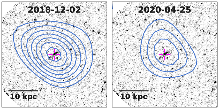
Figure 1: VLA 3-GHz contours of PTF10hgi obtained on November 2, 2018 (left) and April 25, 2020 (right) overlaid on the host galaxy image taken with HST WFC3/UVIS F336W. North is up, and east is to the left. The contours start from $3\sigma$ with $2\sigma$ increments. The crosses represent the SN position. The scale bar shows 10 kpc (4$\farcs$9) at the distance of PTF10hgi.

3 Results

The 3-GHz images taken in the two semesters are shown in Figure 1. Radio emission was significantly detected in both semesters with peak signal-to-noise ratios of 16 and 9 in the former and latter semesters, respectively. The positional uncertainties of peak position were estimated to be $\sim$0$\farcs$3 and $\sim$0$\farcs$5, respectively. The peak position is consistent with the SN location and with previous observations at 3 and 6 GHz within the positional uncertainties (Eftekhari et al., 2019; Law et al., 2019). We conducted a 2-D Gaussian fit to the emission in the image plane, which could not deconvolve source from the synthesized beam in both semesters. Because the emission was spatially unresolved in the observations, we adopted the peak intensity as a source flux density. We found a significant time variability of the radio emission between the two semesters with a 40% decrease in flux density. Note that we found no systematic difference in flux densities of $>$$5\sigma$ sources detected in the same field-of-view in the two semesters. In Figure 2, we plot the flux densities as a function of time together with two previous measurements at 3 GHz by Law et al. (2019) and Mondal et al. (2020). The light curve shows both the rise and decay phases over three years with a peak luminosity of $(2.0\pm 0.2)\times 10^{21}$ W Hz^-1. We searched for other radio observations of PTF10hgi in wide-field radio surveys and in the literature. Schulze et al. (2018) reported a non-detection in the 1.4 GHz data of the NRAO VLA Sky Survey (NVSS; Condon et al., 1998) with a nominal rms level of $\sim$0.45 mJy beam^-1. We also did not find radio emission in the 3 GHz image of the Very Large Array Sky Survey (VLASS; Lacy et al., 2020) observed in March 2019 with an rms noise level of $\sim$0.22 mJy beam^-1. These noise levels are relatively shallow compared to the observations by Eftekhari et al. (2019), Law et al. (2019), Mondal et al. (2020), and in this study, and do not provide useful constraints on the light curve. By using the four data points with radio detection at 3 GHz, we calculated the flux coefficient of variation ($V$; Swinbank et al., 2015), which is equivalent to the fractional variability, defined as $V=s/\bar{F}$, where $s$ is the standard deviation of the flux measurements and $\bar{F}$ is the mean flux density. The calculated fractional variability was $V=0.24$, corresponding to 24% variability in flux density. The maximum-to-median flux density ratio was 1.5. This is the first case of a significant time variability being reported in the late-time radio light curve of a SLSN.

4 Discussion

There are various possibilities for the origin of the variability of radio emission. It is possible that the effects of scintillation could have resulted in the flux changes (e.g., Rickett, 1990). If it were to be the case and the cause of the higher flux density for the first semester, the intrinsic luminosity of the source would be nearly constant. However, it is hard to quantify the effects of scintillation with only four data points. In what follows, we assume the variability is intrinsic to the source and discuss the physical origin related to the SLSN or its host galaxy.

Eftekhari et al. (2019) discussed possible origins for the radio emission, such as star formation activity in the host galaxy, an active galactic nucleus (AGN), interaction between the SN ejecta/jet and CSM, and magnetar wind nebulae. The significant time variability we found in this study enables us to reject the steady radio emission from star-formation activity. We discuss the possibilities of an AGN, shock interaction, and magnetar wind nebulae in the following sections.

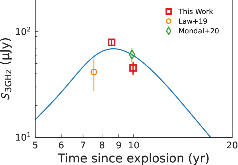
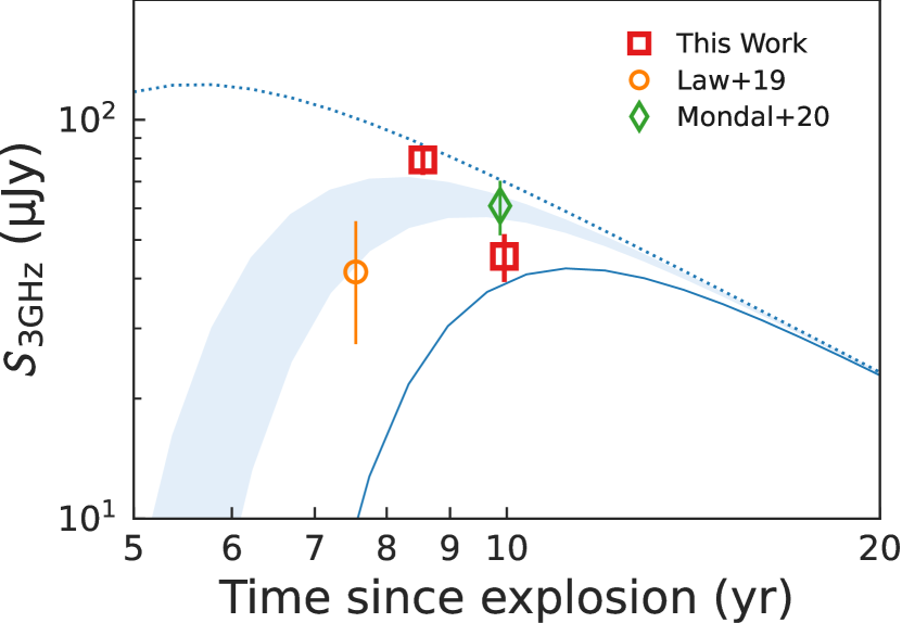
Figure 2: Light curve of PTF10hgi at 3 GHz. Our observed data are presented as squares along with the results of Law et al. (2019) at 3 GHz and Mondal et al. (2020) at 3.3 GHz. The radio emission expected from the star-forming activity in the host galaxy is subtracted from the data points (see text). Left panel: We plot an afterglow model generated using the afterglowpy code (Ryan et al., 2020) with $E_{\rm iso}=1.5\times 10^{54}$ erg and $n=7\times 10^{-3}$ cm^-3. Right panel: We plot the magnetar model presented by Law et al. (2019) with and without free-free absorption as solid and dotted lines, respectively, scaled by a factor of 1.6. The shaded region shows the model with 40–60% of the ejecta singly ionized.

4.1 AGN

The peak position of the radio emission coincides with the SN location and with the center of the host galaxy (Figure 1). Although the optical line diagnostic based on a BPT (Baldwin et al., 1981) diagram shows that the host galaxy lies on the star-forming branch (Leloudas et al., 2015; Perley et al., 2016), it has been reported that the diagram is biased against AGNs in low-mass, blue star-forming galaxies (e.g., Trump et al., 2015). Deep radio surveys have revealed extragalactic variable sources and AGN signatures in faint radio sources (e.g., Mooley et al., 2016; Radcliffe et al., 2019; Smolčić et al., 2017; Algera et al., 2020; Reines et al., 2020). Sarbadhicary et al. (2020) conducted a deep blind survey of radio variables at 1-2 GHz probing down to faint sources ($<$100 $\mu$Jy) on timescales ranging from days to years. They found that 4.9% of radio sources (18 out of 370) have fractional variabilities of $V>0.1$, and their host galaxies show AGN signatures based on thresholds such as X-ray luminosity, mid-infrared colors, optical-to-mm SEDs, and radio excess. Deep radio continuum surveys found that faint sources with radio luminosities or stellar masses similar to those of the PTF10hgi host show AGN features based on various criteria (Smolčić et al., 2017; Algera et al., 2020). A sensitive search for radio emission towards 111 dwarf galaxies ($M_{*}<3\times 10^{9}$ $M_{\odot}$) by Reines et al. (2020) found that 13 galaxies have compact radio sources that are almost certainly AGNs.

Figure 3 compares $V$ with flux density or radio spectral index $\alpha$ (defined as $S_{\nu}\propto\nu^{\alpha}$). The radio spectral index of PTF10hgi was calculated to be $\alpha=-0.14\pm 0.06$ using the data points between 1.2 and 15 GHz obtained in this study and by Eftekhari et al. (2019), Law et al. (2019), and Mondal et al. (2020). Note that we subtracted the expected radio contribution due to star-forming activity from the data points when driving the spectral index, because the radio observations did not spatially resolve the host galaxy. We calculated the radio emission expected from the SFR of 0.15 $M_{\odot}$ yr^-1, which is in between the estimates of Perley et al. (2016) and Schulze et al. (2018): 9.2, 5.4, 3.8, and 2.5 $\mu$Jy at 1.2, 3, 6, and 15 GHz, respectively. Figure 3 shows that PTF10hgi shares a similar region to those of moderate-variability sources ($V>0.1$) found in the survey of Sarbadhicary et al. (2020). Mondal et al. (2020) obtained a flat spectrum of PTF10hgi in the frequency range 1.2–15 GHz and an upper limit at 0.6 GHz. Figure 4 shows the radio spectrum of PTF10hgi. The spectral features are similar to those of flat-spectrum sources or gigahertz-peaked-spectrum (GPS) sources, which have radio spectra with peak frequencies of a few GHz (O’Dea, 1998, for a review). Their spectral shape may arise from compact cores and jets due to self-absorbed synchrotron emission. It was found that the linear source size is negatively correlated with turnover frequency in their spectra (O’Dea, 1998), giving a linear size of $\sim$100-500 pc for sources with peaks at $\sim$1–3 GHz, which is consistent with the upper limit obtained in 6-GHz observations of PTF10hgi ($\lesssim$2 kpc; Eftekhari et al., 2019). These sources are thought to represent the early stages of the evolution of radio AGN, confinement to small spatial scales by a dense interstellar medium, or intermittent phases of AGN activity. They are typically bright radio sources, but it is expected that a large population of low-luminosity sources exist, which are yet to be explored (e.g., Collier et al., 2018).

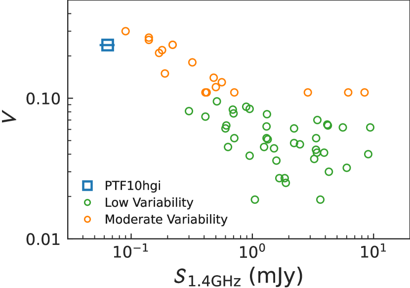
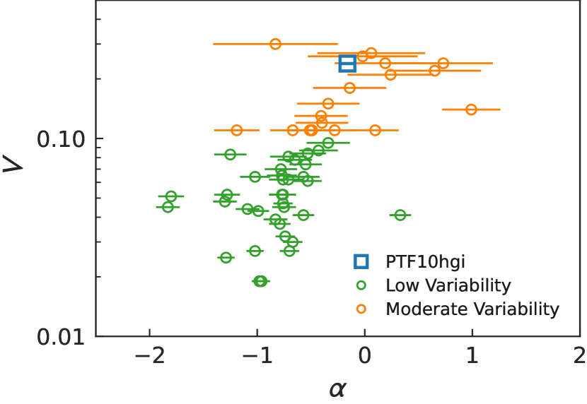
Figure 3: Left panel: Comparison between 1.4 GHz flux density and flux coefficient of variation $V$. The flux density of PTF10hgi is taken from the measured by Mondal et al. (2020) at 1.2 GHz. Radio variable sources with ‘moderate-variability’ ($V>0.1$) and ‘low-variability’ ($V<0.1$) found by Sarbadhicary et al. (2020) are plotted for comparison. Right panel: Comparison between radio spectral index $\alpha$ and $V$. The spectral index was measured at 1.2–15 GHz for PTF10hgi and at 1.4–3 GHz for the sample of radio variable sources by Sarbadhicary et al. (2020).

4.2 Interaction between SN Outflow and CSM

Eftekhari et al. (2019) discussed the external shock interaction between SN outflow and CSM as the origin of radio emission. They considered two scenarios: non-relativistic (quasi-)spherical SN ejecta and an off-axis relativistic jet. For the spherical SN ejecta scenario, they investigated the ejecta velocity and mass-loss rate based on the phase-space of peak luminosity versus peak time assuming that the radio observations were conducted around the peak time. The inferred values are significantly different from those of known radio-emitting SNe Ib/c, and they concluded that this scenario is unlikely.

The other scenario is that the radio emission is an afterglow arising from an initially off-axis jet that decelerated and spread into the line of sight at late times. They generated afterglow models for a range of jet energies and CSM densities and found that the observed 6-GHz flux density measured approximately 7.5 years after the explosion can be reproduced with an isotropic-equivalent energy $E_{\rm iso}\sim$ (3-5) $\times 10^{53}$ erg and CSM densities $n\sim 10^{-3}$–$10^{2}$ cm^-3. Now that we have more data points that show the time variability, we can examine whether the light curve can be explained by afterglow models. We utilize the publicly available afterglowpy code (Ryan et al., 2020), which generates afterglow light curves using semianalytic approximations of the jet evolution and synchrotron emission. We adopted a top hat jet with following fixed parameters: jet opening angle of $10^{\circ}$, electron energy distribution index of $p=2.5$, thermal energy fraction in electrons of $\epsilon_{e}=0.1$, and thermal energy fraction in magnetic field of $\epsilon_{B}=0.01$, which are typical values for GRBs (e.g., Wang et al., 2015); these values were also assumed by Eftekhari et al. (2019) and Eftekhari et al. (2020). The left panel of Figure 2 shows a model light curve along with the radio data. We found that the data points can be reproduced with $E_{\rm iso}\approx 10^{54}$ erg, $n\approx 10^{-2}$ cm^-3, and a viewing angle of $\theta_{\rm obs}=60^{\circ}$. The inferred energy is in the highest range of GRBs (e.g., Butler et al., 2010; Wang et al., 2015). Coppejans et al. (2018) compiled all radio observations of SLSNe-I and constrained energies and mass-loss rates or CSM densities for off-axis jets, but lower-density environments ($n\lesssim 10^{-2}$ cm^-3) with larger viewing angles were not ruled out. However, the spectral index of the afterglow model, $(1-p)/2$ ($p>2$), is inconsistent with the observed flat radio spectrum. Even if we consider the time evolution of the spectral index of an afterglow (Sari et al., 1998), it is difficult to reproduce the flat spectrum.

4.3 Magnetar Wind Nebula

PTF10hgi has been proposed to be a magnetar-powered SLSN (Eftekhari et al., 2019; Law et al., 2019; Mondal et al., 2020). Eftekhari et al. (2019) argued that the properties of the source are consistent with a magnetar wind nebula, and its timescale or luminosity can be reproduced by scaling the magnetar model for the persistent radio source associated with the repeating FRB 121102 (Metzger et al., 2017). Law et al. (2019) detected radio emission in VLA 3-GHz observations and found that the emission is consistent with the interpretation that it is powered by a magnetar with free-free absorption in partially ionized ejecta. They calculated the time evolution of radio emission from the pulsar wind nebulae (PWNe) based on the model of Murase et al. (2015) and Murase et al. (2016). Murase et al. (2016) showed that under their model, pulsar-driven SN remnants cause quasi-steady synchrotron radio emission associated with non-thermal electron-positron pairs in nascent PWNe on a timescale of decades. Based on this model, Law et al. (2019) estimated the initial parameters of a magnetar (spin period $P_{i}$, magnetic field $B$, and ejecta mass $M_{\rm ej}$) by fitting the early optical light curve. They assumed an electron-positron injection spectrum motivated by Galactic PWNe, such as the Crab PWN (e.g. Tanaka & Takahara, 2010, 2013), a broken power law with a peak Lorentz factor of $\gamma_{b}=10^{5}$, and injection spectral indices of $q_{1}=1.5$ and $q_{2}=2.5$. They found that a model with ($P_{i}$, $B$, $M_{\rm ej}$) = (1 ms, $1.4\times 10^{13}$ G, 15 $M_{\odot}$) and 30–50% of the ejecta singly ionized can reproduce the observed data at 3 and 6 GHz.

In the right panel of Figure 2, we plot the magnetar model presented by Law et al. (2019) with the same initial parameters. We found that this model with 40–60% of the ejecta singly ionized and scaled by a factor of 1.6 in the vertical direction can reproduce the observed light curve. The increase of flux density by a factor of 1.6 can be achieved by a slight modification of the parameters, such as a $\sim$30% decrease of the magnetic field. The timescale of the declining phase appears to be shorter than that of the model. One possibility is a rapid spin-down of a young pulsar by the loss of rotational energy due to not only magnetic dipole radiation but also dissipation processes (e.g., Maeda et al., 2007). Alternatively, a steeper spectral injection index would cause a rapid decline. However, a larger $q_{1}$ yields a steeper spectrum, which is inconsistent with the flat spectrum in the range of 1–15 GHz (Mondal et al., 2020). Figure 4 shows the radio spectrum of PTF10hgi along with the same magnetar model as in Figure 2 by changing observation epochs. We divided the data set into three epochs to see the time variability of the spectral index in Figure 4. We found no significant change between the epochs of October 2017–January 2018 ($\alpha=0.07\pm 0.54$) and December 2019–April 2020 ($\alpha=-0.08\pm 0.07$), although the power-law fitting results are not stringent. It is difficult to compare with the data of December 2018 due to its limited number of points. The model significantly underpredicts the 15-GHz flux, as noted by Mondal et al. (2020) and Eftekhari et al. (2020). A shallower spectral injection index could be a solution for reproducing the flatter spectrum (Mondal et al., 2020). This may suggest a need for modifying the standard model of PWNe (e.g., Ishizaki et al., 2017). To constrain the models and parameters, multi-frequency long-term monitoring is required.

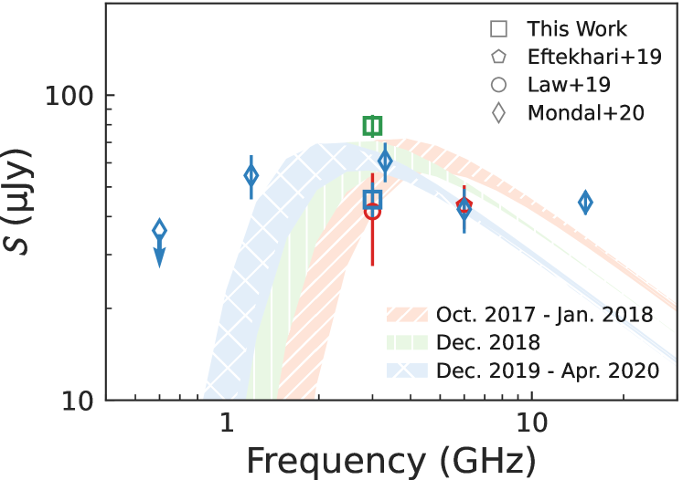
Figure 4: Radio spectra of PTF10hgi. The observed data are taken from our results and the literature (Eftekhari et al., 2019; Law et al., 2019; Mondal et al., 2020). Radio emission expected from the star-forming activity in the host galaxy was subtracted from the data. We plot the magnetar model presented by Law et al. (2019) scaled by a factor of 1.6 with free-free absorption 40–60% of the ejecta singly ionized. The data points and models are color-coded by their observation epochs.

5 Conclusions

We conducted VLA 3-GHz observations of SLSN-I PTF10hgi ($z=0.0987$) 8.6 and 10 years after its explosion. Radio emission was significantly detected in both epochs. We found a time variability with a $\sim$40% decrease in flux density in the second epoch. Through combination with previous measurements in two other epochs, we constrained both the rise and decay phases of a radio light curve over three years peaking at approximately 8–9 years after the explosion. This is the first report of variability of a late-time radio light curve in a SLSN. A possible scenario for the origin of the variability is a low-luminosity AGN in the host galaxy. Another possibility is an afterglow caused by the interaction between an off-axis jet and CSM. Comparison with models shows that although the light curve can be reproduced, the predicted radio spectrum is inconsistent with the observed flat spectrum. Alternatively, we found that the light curve can be reproduced by a magnetar wind nebula model. Our findings provide important implications for the central engine of SLSNe.

Current data sets are not enough to make definitive settlements on PTF10hgi, and more data at different times and frequencies are required. A decrease in flux density on a long timescale would be favored for the central engine scenarios, because fluctuations of observed flux density can be caused by AGN activity or scintillation. While a flat spectrum can be explained by AGN or magnetar scenarios, a steeper spectral index is expected for afterglow models. Because a time evolution of spectral index could also happen in magnetar wind nebula models (Murase et al., 2016; Omand et al., 2018), long-term monitoring with multi-frequencies are important.

References

- Algera et al. (2020) Algera, H. S. B., van der Vlugt, D., Hodge, J. A., et al. 2020, The Astrophysical Journal, 903, 139, doi: 10.3847/1538-4357/abb77a
- Baldwin et al. (1981) Baldwin, J. A., Phillips, M. M., & Terlevich, R. 1981, Publications of the Astronomical Society of the Pacific, 93, 5, doi: 10.1086/130766
- Butler et al. (2010) Butler, N. R., Bloom, J. S., & Poznanski, D. 2010, The Astrophysical Journal, 711, 495, doi: 10.1088/0004-637X/711/1/495
- Chabrier (2003) Chabrier, G. 2003, Publications of the Astronomical Society of the Pacific, 115, 763, doi: 10.1086/376392
- Chevalier & Irwin (2011) Chevalier, R. A., & Irwin, C. M. 2011, The Astrophysical Journal, 729, L6, doi: 10.1088/2041-8205/729/1/L6
- Collier et al. (2018) Collier, J. D., Tingay, S. J., Callingham, J. R., et al. 2018, Monthly Notices of the Royal Astronomical Society, 477, 578, doi: 10.1093/mnras/sty564
- Condon et al. (1998) Condon, J. J., Cotton, W. D., Greisen, E. W., et al. 1998, The Astronomical Journal, 115, 1693, doi: 10.1086/300337
- Coppejans et al. (2018) Coppejans, D. L., Margutti, R., Guidorzi, C., et al. 2018, The Astrophysical Journal, 856, 56, doi: 10.3847/1538-4357/aab36e
- Dexter & Kasen (2013) Dexter, J., & Kasen, D. 2013, The Astrophysical Journal, 772, 30, doi: 10.1088/0004-637X/772/1/30
- Eftekhari et al. (2019) Eftekhari, T., Berger, E., Margalit, B., et al. 2019, The Astrophysical Journal, 876, L10, doi: 10.3847/2041-8213/ab18a5
- Eftekhari et al. (2020) Eftekhari, T., Margalit, B., Omand, C. M. B., et al. 2020, arXiv:2010.06612 [astro-ph]. https://arxiv.org/abs/2010.06612
- Gal-Yam (2012) Gal-Yam, A. 2012, Science, 337, 927, doi: 10.1126/science.1203601
- Greiner et al. (2015) Greiner, J., Mazzali, P. A., Kann, D. A., et al. 2015, Nature, 523, 189, doi: 10.1038/nature14579
- Hatsukade et al. (2018) Hatsukade, B., Tominaga, N., Hayashi, M., et al. 2018, The Astrophysical Journal, 857, 72, doi: 10.3847/1538-4357/aab616
- Inserra et al. (2013) Inserra, C., Smartt, S. J., Jerkstrand, A., et al. 2013, The Astrophysical Journal, 770, 128, doi: 10.1088/0004-637X/770/2/128
- Ishizaki et al. (2017) Ishizaki, W., Tanaka, S. J., Asano, K., & Terasawa, T. 2017, The Astrophysical Journal, 838, 142, doi: 10.3847/1538-4357/aa679b
- Kasen & Bildsten (2010) Kasen, D., & Bildsten, L. 2010, The Astrophysical Journal, 717, 245, doi: 10.1088/0004-637X/717/1/245
- Lacy et al. (2020) Lacy, M., Baum, S. A., Chandler, C. J., et al. 2020, Publications of the Astronomical Society of the Pacific, 132, 035001, doi: 10.1088/1538-3873/ab63eb
- Law et al. (2019) Law, C. J., Omand, C. M. B., Kashiyama, K., et al. 2019, The Astrophysical Journal, 886, 24, doi: 10.3847/1538-4357/ab4adb
- Leloudas et al. (2015) Leloudas, G., Hsiao, E. Y., Johansson, J., et al. 2015, Astronomy & Astrophysics, 574, A61, doi: 10.1051/0004-6361/201322035
- Lunnan et al. (2014) Lunnan, R., Chornock, R., Berger, E., et al. 2014, The Astrophysical Journal, 787, 138, doi: 10.1088/0004-637X/787/2/138
- Maeda et al. (2007) Maeda, K., Tanaka, M., Nomoto, K., et al. 2007, The Astrophysical Journal, 666, 1069, doi: 10.1086/520054
- Margalit et al. (2018) Margalit, B., Metzger, B. D., Thompson, T. A., Nicholl, M., & Sukhbold, T. 2018, Monthly Notices of the Royal Astronomical Society, 475, 2659, doi: 10.1093/mnras/sty013
- McMullin et al. (2007) McMullin, J. P., Waters, B., Schiebel, D., Young, W., & Golap, K. 2007, 376, 127
- Metzger et al. (2017) Metzger, B. D., Berger, E., & Margalit, B. 2017, The Astrophysical Journal, 841, 14, doi: 10.3847/1538-4357/aa633d
- Metzger et al. (2015) Metzger, B. D., Margalit, B., Kasen, D., & Quataert, E. 2015, Monthly Notices of the Royal Astronomical Society, 454, 3311, doi: 10.1093/mnras/stv2224
- Mondal et al. (2020) Mondal, S., Bera, A., Chandra, P., & Das, B. 2020, Monthly Notices of the Royal Astronomical Society, 498, 3863, doi: 10.1093/mnras/staa2637
- Mooley et al. (2016) Mooley, K. P., Hallinan, G., Bourke, S., et al. 2016, The Astrophysical Journal, 818, 105, doi: 10.3847/0004-637X/818/2/105
- Murase et al. (2015) Murase, K., Kashiyama, K., Kiuchi, K., & Bartos, I. 2015, The Astrophysical Journal, 805, 82, doi: 10.1088/0004-637X/805/1/82
- Murase et al. (2016) Murase, K., Kashiyama, K., & Mészáros, P. 2016, Monthly Notices of the Royal Astronomical Society, 461, 1498, doi: 10.1093/mnras/stw1328
- Nicholl et al. (2016) Nicholl, M., Berger, E., Smartt, S. J., et al. 2016, The Astrophysical Journal, 826, 39, doi: 10.3847/0004-637X/826/1/39
- O’Dea (1998) O’Dea, C. P. 1998, Publications of the Astronomical Society of the Pacific, 110, 493, doi: 10.1086/316162
- Omand et al. (2018) Omand, C. M. B., Kashiyama, K., & Murase, K. 2018, Monthly Notices of the Royal Astronomical Society, 474, 573, doi: 10.1093/mnras/stx2743
- Perley et al. (2016) Perley, D. A., Quimby, R. M., Yan, L., et al. 2016, The Astrophysical Journal, 830, 13, doi: 10.3847/0004-637X/830/1/13
- Perley & Butler (2017) Perley, R. A., & Butler, B. J. 2017, The Astrophysical Journal Supplement Series, 230, 7, doi: 10.3847/1538-4365/aa6df9
- Planck Collaboration et al. (2020) Planck Collaboration, Aghanim, N., Akrami, Y., et al. 2020, Astronomy and Astrophysics, 641, A6, doi: 10.1051/0004-6361/201833910
- Quimby et al. (2010) Quimby, R. M., Kulkarni, S., Ofek, E., et al. 2010, The Astronomer’s Telegram, 2740
- Radcliffe et al. (2019) Radcliffe, J. F., Beswick, R. J., Thomson, A. P., et al. 2019, Monthly Notices of the Royal Astronomical Society, 490, 4024, doi: 10.1093/mnras/stz2748
- Reines et al. (2020) Reines, A. E., Condon, J. J., Darling, J., & Greene, J. E. 2020, The Astrophysical Journal, 888, 36, doi: 10.3847/1538-4357/ab4999
- Rickett (1990) Rickett, B. J. 1990, Annual Review of Astronomy and Astrophysics, 28, 561, doi: 10.1146/annurev.aa.28.090190.003021
- Ryan et al. (2020) Ryan, G., van Eerten, H., Piro, L., & Troja, E. 2020, The Astrophysical Journal, 896, 166, doi: 10.3847/1538-4357/ab93cf
- Sarbadhicary et al. (2020) Sarbadhicary, S. K., Tremou, E., Stewart, A. J., et al. 2020, arXiv e-prints, 2009, arXiv:2009.05056
- Sari et al. (1998) Sari, R., Piran, T., & Narayan, R. 1998, The Astrophysical Journal Letters, 497, L17, doi: 10.1086/311269
- Schulze et al. (2018) Schulze, S., Krühler, T., Leloudas, G., et al. 2018, Monthly Notices of the Royal Astronomical Society, 473, 1258, doi: 10.1093/mnras/stx2352
- Smolčić et al. (2017) Smolčić, V., Delvecchio, I., Zamorani, G., et al. 2017, Astronomy & Astrophysics, 602, A2, doi: 10.1051/0004-6361/201630223
- Swinbank et al. (2015) Swinbank, J. D., Staley, T. D., Molenaar, G. J., et al. 2015, Astronomy and Computing, 11, 25, doi: 10.1016/j.ascom.2015.03.002
- Tanaka & Takahara (2010) Tanaka, S. J., & Takahara, F. 2010, The Astrophysical Journal, 715, 1248, doi: 10.1088/0004-637X/715/2/1248
- Tanaka & Takahara (2013) —. 2013, Monthly Notices of the Royal Astronomical Society, 429, 2945, doi: 10.1093/mnras/sts528
- Trump et al. (2015) Trump, J. R., Sun, M., Zeimann, G. R., et al. 2015, The Astrophysical Journal, 811, 26, doi: 10.1088/0004-637X/811/1/26
- Wang et al. (2015) Wang, X.-G., Zhang, B., Liang, E.-W., et al. 2015, The Astrophysical Journal Supplement Series, 219, 9, doi: 10.1088/0067-0049/219/1/9
- Woosley et al. (2007) Woosley, S. E., Blinnikov, S., & Heger, A. 2007, Nature, 450, 390, doi: 10.1038/nature06333