How Alfvén waves energize the solar wind: heat vs work

Abstract

A growing body of evidence suggests that the solar wind is powered to a large extent by an Alfvén-wave (AW) energy flux. AWs energize the solar wind via two mechanisms: heating and work. We use high-resolution direct numerical simulations of reflection-driven AW turbulence (RDAWT) in a fast-solar-wind stream emanating from a coronal hole to investigate both mechanisms. In particular, we compute the fraction of the AW power at the coronal base ($P_{\rm AWb}$) that is transferred to solar-wind particles via heating between the coronal base and heliocentric distance $r$, which we denote $\chi_{\rm H}(r)$, and the fraction that is transferred via work, which we denote $\chi_{\rm W}(r)$. We find that $\chi_{\rm W}(r_{\rm A})$ ranges from 0.15 to 0.3, where $r_{\rm A}$ is the Alfvén critical point. This value is small compared to one because the Alfvén speed $v_{\rm A}$ exceeds the outflow velocity $U$ at $r<r_{\rm A}$, so the AWs race through the plasma without doing much work. At $r>r_{\rm A}$, where $v_{\rm A}<U$, the AWs are in an approximate sense “stuck to the plasma,” which helps them do pressure work as the plasma expands. However, much of the AW power has dissipated by the time the AWs reach $r=r_{\rm A}$, so the total rate at which AWs do work on the plasma at $r>r_{\rm A}$ is a modest fraction of $P_{\rm AWb}$. We find that heating is more effective than work at $r<r_{\rm A}$, with $\chi_{\rm H}(r_{\rm A})$ ranging from 0.5 to 0.7. The reason that $\chi_{\rm H}\geq 0.5$ in our simulations is that an appreciable fraction of the local AW power dissipates within each Alfvén-speed scale height in RDAWT, and there are a few Alfvén-speed scale heights between the coronal base and $r_{\rm A}$. A given amount of heating produces more magnetic moment in regions of weaker magnetic field. Thus, paradoxically, the average proton magnetic moment increases robustly with increasing $r$ at $r>r_{\rm A}$, even though the total rate at which AW energy is transferred to particles at $r>r_{\rm A}$ is a small fraction of $P_{\rm AWb}$.

1 Introduction

Following Parker’s (1958) prediction that the Sun emits a supersonic wind, a number of studies attempted to model the solar wind as a spherically symmetric outflow powered by the outward conduction of heat from a hot coronal base (e.g. Parker, 1965; Hartle & Sturrock, 1968; Durney, 1972; Roberts & Soward, 1972). Although these studies obtained supersonic wind solutions, they were unable to reproduce the large outflow velocities measured in the fast solar wind near Earth ($700-800\mbox{ km}\mbox{ s}^{-1}$), and they did not explain the origin of the high coronal temperatures ($\sim 10^{6}\mbox{ K}$) upon which the models were based.

These shortcomings led a number of authors to conjecture that the solar wind is powered to a large extent by an energy flux carried by waves. Several observations support this idea, including in situ measurements of large-amplitude, outward-propagating Alfvén waves (AWs) in the interplanetary medium (e.g., Belcher & Davis, 1971; Tu & Marsch, 1995; Bruno & Carbone, 2013) and remote observations of AW-like motions in the low corona that carry an energy flux sufficient to power the solar wind (De Pontieu et al., 2007).

These observations have stimulated numerous theoretical investigations of how AWs might heat and accelerate the solar wind (see, e.g., Hansteen & Velli, 2012, and references therein). In many of these models, a substantial fraction of the Sun’s AW energy flux is transferred to solar-wind particles by some form of dissipation. Because photospheric motions primarily launch large-wavelength AWs, and because large-wavelength AWs are virtually dissipationless, the AWs are unable to transfer their energy to the plasma near the Sun unless they become turbulent. Turbulence dramatically enhances the rate of AW dissipation because it causes AW energy to cascade from large wavelengths to small wavelengths where dissipation is rapid. One of the dominant nonlinearities that gives rise to AW turbulence is the interaction between counter-propgating AWs (Iroshnikov, 1963; Kraichnan, 1965). Because the Sun launches only outward-propagating waves, solar-wind models that invoke this nonlinearity require some source of inward-propagating AWs. One such source is AW reflection arising from the radial variation in the Alfvén speed (Heinemann & Olbert, 1980; Velli, 1993; Hollweg & Isenberg, 2007). Direct numerical simulations of reflection-driven AW turbulence (RDAWT) in a fast-solar-wind stream emanating from a coronal hole (Perez & Chandran, 2013; van Ballegooijen & Asgari-Targhi, 2016, 2017; Chandran & Perez, 2019) have shown that AW turbulence initiated by wave reflections can drive a vigorous turbulent cascade. The turbulent dissipation rates in the simulations of Perez & Chandran (2013) and Chandran & Perez (2019) are consistent with the turbulent heating rates in solar-wind models that rely on RDAWT, which have proven quite successful at explaining solar-wind observations (Cranmer et al., 2007; Verdini et al., 2010; Chandran et al., 2011; van der Holst et al., 2014; Usmanov et al., 2014). (We note that there are a number of alternative approaches to incorporating AWs into solar-wind models — see, e.g., Suzuki & Inutsuka, 2006; Suzuki, 2006; Ofman, 2010; Shoda et al., 2019).

In addition to solar-wind heating via the cascade and dissipation of AW energy, AWs energize the solar wind through the work done by the AW pressure force, which directly accelerates plasma away from the Sun (e.g., Hollweg, 1973; Wang, 1993). The relative importance of AW heating and AW work, however, is not well understood. Our goal in this paper is to use direct numerical simulations of RDAWT to determine the fraction of the AW power that is transferred to the solar wind via turbulent dissipation between the coronal base and radius $r$, denoted $\chi_{\rm H}(r)$, and the fraction that is transferred via work, $\chi_{\rm W}(r)$.

In Section 2, we present the mathematical framework that we use to address this problem and derive mathematical expressions for $\chi_{\rm H}(r)$ and $\chi_{\rm W}(r)$. In Section 3 we compute $\chi_{\rm H}(r)$ and $\chi_{\rm W}(r)$ using high-resolution numerical simulations of RDAWT with fixed, observationally constrained, model radial profiles for the plasma density, solar-wind outflow velocity, and background magnetic-field strength. We compare our numerical results with the values of $\chi_{\rm H}(r)$ and $\chi_{\rm W}(r)$ that result from a previously published analytic model of RDAWT (Chandran & Hollweg, 2009). We also investigate the radial evolution of the average proton magnetic moment $k_{\rm B}T_{\perp\rm p}(r)/B(r)$ when RDAWT is the dominant proton heating mechanism, where $T_{\perp\rm p}$ is the perpendicular proton temperature, $k_{\rm B}$ is the Boltzmann constant, and $B$ is the magnetic-field strength.

2 Energization of the solar wind by AW turbulence

We consider turbulent fluctuations within a narrow magnetic flux tube of cross-sectional area $a(r)\ll r^{2}$, where $r$ is heliocentric distance. We neglect solar rotation and take this flux tube to be centered on a radial magnetic-field line. We take the density $\rho$, solar-wind outflow velocity $\bm{U}$, and background magnetic field $\bm{B}_{0}$ to be fixed functions of $r$,

$$\rho=\rho(r),\quad\bm{U} = U(r)\mathbf{\hat{b}},\quad\bm{B}_{0}=B_{0}(r)\mathbf{\hat{b}},$$ (1)

where $\mathbf{\hat{b}}\equiv\mathbf{B}_{0}/B_{0}$. Magnetic-flux conservation implies that

$$a(r)=\frac{B_{\odot}}{B_{0}(r)}a_{\odot},$$ (2)

where $a_{\odot}$ and $B_{\odot}$ are the values of $a(r)$ and $B(r)$ at the coronal base, located at $r\simeq R_{\odot}$, where $R_{\odot}$ is the solar radius. We allow for super-radial expansion of the magnetic field, but assume that $a/r^{2}$ is small enough that $\mathbf{\hat{b}}$ is nearly radial and $r-R_{\odot}$ is approximately equal to distance from the coronal base measured along the magnetic field. We also assume that the fluctuations in the velocity and magnetic field, denoted $\delta\bm{v}$ and $\delta\bm{B}$, are orthogonal to $\bm{B}_{0}$, that $\delta\bm{v}$ is divergence-free, and that density fluctuations are negligibly small.

Given these simplifying assumptions, the fluctuations satisfy the equations (see, e.g., Cranmer & van Ballegooijen, 2005; Verdini & Velli, 2007; Chandran & Hollweg, 2009)

$$\frac{\partial\mathbf{z}^{\pm}}{\partial t}+\left(U\pm v_{A}\right)\frac{\partial\mathbf{z}^{\pm}}{\partial r}+\left(U\mp v_{A}\right)\left(\frac{1}{4H_{\rho}}\mathbf{z}^{\pm}-\frac{1}{2H_{A}}\mathbf{z}^{\mp}\right)=-\left(\mathbf{z}^{\mp}\cdot\mathbf{\nabla}\mathbf{z}^{\pm}-\frac{\nabla P}{\rho}\right)+\bm{D}^{\pm},$$ (3)

where $\mathbf{z}^{\pm}=\delta\mathbf{v}\mp\delta\mathbf{b}$ are the Elsasser variables, $\delta\mathbf{v}$ is the fluctuating velocity, $\delta\mathbf{b}=\delta\mathbf{B}/\sqrt{4\pi\rho}$ is the fluctuating Alfvén velocity, $v_{\rm A}=B_{0}/\sqrt{4\pi\rho}$ is the Alfvén speed, $P=p+B^{2}/8\pi$ is the combined plasma and magnetic pressure, $\bm{D}^{\pm}$ is a dissipation term that accounts for viscosity and resistivity (or possibly hyper-viscosity and hyper-resistivity in some numerical models), and

$$\frac{1}{H_{\rho}}\equiv-\frac{1}{\rho}\frac{\mathrm{d}\rho}{\mathrm{d}r},\quad\frac{1}{H_{B}}\equiv-\frac{1}{B_{0}}\frac{\mathrm{d}B_{0}}{\mathrm{d}r},\quad\hbox{and}\quad\frac{1}{H_{A}}\equiv\frac{1}{v_{A}}\frac{\mathrm{d}v_{\rm A}}{\mathrm{d}r}=\frac{1}{2H_{\rho}}-\frac{1}{H_{B}}$$ (4)

are characteristic length scales of $\rho$, $B_{0}$ and $v_{\rm A}$ along the magnetic field, respectively. Our definition of Elsasser variables with the “$\mp$” sign convention implies that $\mathbf{z}^{+}$ ($\mathbf{z}^{-}$) represents AW fluctuations propagating parallel (anti-parallel) to $\bm{B}_{0}$ in the local plasma frame. For concreteness, we take $\bm{B}_{0}$ to point radially outward from the Sun so that $\bm{z}^{+}$ ($\bm{z}^{-}$) represents AW fluctuations that propagate anti-sunward (sunward) in the plasma frame. Equations (3) can be also seen as an inhomogeneous version of the reduced magnetohydrodynamics (RMHD) model (Kadomtsev & Pogutse, 1974; Strauss, 1976) with an important new piece of physics, namely the linear coupling between $\mathbf{z}^{+}$ and $\mathbf{z}^{-}$ fluctuations that is responsible for the non-WKB reflection of AWs resulting from the spatial variation of $v_{\rm A}$.

2.1 Solar wind energization: how the AW power decreases with $r$

The background flow and turbulent fluctuations satisfy a total-energy conservation relation, which, in steady state, takes the form (Chandran et al., 2015)

$$\mathbf{\nabla}\cdot\left[(F_{\rm flow}+F_{\rm turb})\bm{\hat{b}}\right]=0,$$ (5)

where

$$F_{\rm flow}=\frac{\rho U^{3}}{2}+\frac{\gamma Up}{\gamma-1}-\frac{GM_{\odot}\rho U}{r}+q_{r}$$ (6)

is the enthalpy flux of the background plasma, $G$ is the universal gravitational constant, $M_{\odot}$ is the mass of the sun, $\gamma$ is the ratio of specific heats, $q_{r}$ is the radial component of the heat flux,

$$F_{\rm turb}(r)=F^{+}(r)+F^{-}(r)+U(r)p_{\rm w}(r)$$ (7)

is the enthalpy flux of the fluctuations,

$$F^{\pm}(r)\equiv\left[U(r)\pm v_{\rm A}(r)\right]\mathcal{E}^{\pm}(r)$$ (8)

is the energy flux of the Elsasser field $\mathbf{z}^{\pm}$,

$$\mathcal{E}^{\pm}(r)\equiv\left\langle\frac{1}{4}\rho|\mathbf{z}^{\pm}|^{2}\right\rangle=\frac{1}{4}\rho(r)[z_{\rm rms}^{\pm}(r)]^{2}$$ (9)

is the average energy density of Elsasser field $\mathbf{z}^{\pm}$, $\left\langle\cdots\right\rangle$ denotes a statistical ensemble average, rms denotes the root-mean-square (rms) value,

$$p_{\rm w}(r)=\frac{1}{2}\left[{\mathcal{E}}^{+}(r)+{\mathcal{E}}^{-}(r)-{\cal E}_{\rm R}(r)\right]=\frac{\delta B_{\rm rms}^{2}(r)}{8\pi}$$ (10)

is the magnetic pressure of the fluctuations, and

$$\mathcal{E}_{\rm R}(r)\equiv\left\langle\frac{1}{2}\rho\bm{z}^{+}\cdot\bm{z}^{-}\right\rangle=\frac{1}{2}\rho(r)\left[\delta v_{\rm rms}^{2}(r)-\frac{\delta B^{2}_{\rm rms}(r)}{4\pi\rho(r)}\right]$$ (11)

is the average residual energy density.

Upon taking the dot product of equation (3) with $\rho\mathbf{z}^{\pm}/2$, performing an ensemble average, and summing the $+$ and $-$ versions of the equation, we obtain a separate equation describing the evolution of the fluctuation energy in steady state,

$$\mathbf{\nabla}\cdot[(F^{+}+F^{-})\bm{\hat{b}}]=-p_{\rm w}\mathbf{\nabla}\cdot(\bm{\hat{b}}U)-\sigma U\mathcal{E}_{\rm R}-Q,$$ (12)

where

$$Q=\left\langle\frac{1}{2}\rho(\mathbf{z}^{+}\cdot\mathbf{D}^{+}+\mathbf{z}^{-}\cdot\mathbf{D}^{-})\right\rangle$$ (13)

is the average turbulent heating rate, and $\sigma=\nabla\cdot\mathbf{\hat{b}}=1/H_{B}$. When ${\mathcal{E}}_{\rm R}\rightarrow 0$, ${\mathcal{E}}^{-}/{\mathcal{E}}^{+}\rightarrow 0$, and $Q\rightarrow 0$, (12) reduces to Equation (42) of Dewar (1970), which is equivalent to the statement that the action of outward-propagating AWs is conserved. Combining (7) and (12), we obtain the relation

$$\mathbf{\nabla}\cdot(F_{\rm turb}\bm{\hat{b}})=\frac{1}{a(r)}\frac{\mathrm{d}P_{\rm AW}}{\mathrm{d}r}=-\sigma U{\mathcal{E}}_{\rm R}+U\frac{\mathrm{d}p_{\rm w}}{\mathrm{d}r}-Q,$$ (14)

where

$$P_{\rm AW}(r)=a(r)F_{\rm turb}(r)$$ (15)

is the AW power. For the solar case, in which ${\mathcal{E}}^{+}>{\mathcal{E}}^{-}$ and $P_{\rm AW}>0$, (14) describes how the AW power decreases with increasing $r$. Equation (5) implies that $P_{\rm AW}(r)+P_{\rm flow}(r)$ is independent of $r$, where $P_{\rm flow}=a(r)F_{\rm flow}(r)$ is the power carried by the outflowing background plasma. Thus, as $P_{\rm AW}$ decreases, $P_{\rm flow}$ increases, and energy is transferred from the AW fluctuations to the background without loss.

By multiplying (14) by $a(r)$ and integrating from the coronal base at $r=r_{\rm b}$ out to radius $r$ we obtain

$$P_{\rm AW}(r)-P_{\rm AWb}=\int_{r_{\rm b}}^{r}a(r^{\prime})U(r^{\prime})\left[\frac{\mathrm{d}}{\mathrm{d}r^{\prime}}p_{\rm w}(r^{\prime})-\sigma(r^{\prime})\mathcal{E}_{\rm R}(r^{\prime})\right]\textrm{d}r^{\prime}-\int_{r_{\rm b}}^{r}a(r^{\prime})Q(r^{\prime})\textrm{d}r^{\prime},$$ (16)

where the “b” subscript indicates that the subscripted quantity ($P_{\rm AW}$ in this case) is evaluated at $r=r_{\rm b}$. The first term inside the first integral of Equation (16) is the negative of the radial component of the pressure force on a plasma parcel of thickness $dr$, $-a(\textrm{d}p_{\rm w}/\textrm{d}r)dr$, multiplied by the radial velocity $U$, which has the familiar force-times-velocity form of mechanical power and represents the rate at which $P_{\rm AW}$ decreases with increasing radius due to the work done by AWs on the flow. When residual energy $\mathcal{E}_{\rm R}$ is negative, which has been shown to result from the nonlinear interaction of counter-propagating AWs (Müller & Grappin, 2005; Boldyrev et al., 2011; Wang et al., 2011), the second term in the first integral results in a small reduction of the net work done by the AW pressure. However, positive residual energy is possible in RDAWT when linear terms responsible for non-WKB reflection dominate nonlinear terms and when $\textrm{d}v_{\rm A}/\textrm{d}r>0$, in which case the residual energy will be responsible for a slight increase in the net work done by the AW pressure. The second integral in Equation (16) represents the rate of decrease in $P_{\rm AW}$ due to dissipation and turbulent heating. We rewrite Equation (16) as

$$P_{\rm AW}(r)-P_{\rm AWb}=-H(r)-W(r),$$ (17)

where

$$H(r) = \int_{\rm r_{\rm b}}^{r}a(r^{\prime})Q(r^{\prime})\textrm{d}r^{\prime}$$ (18)

$$\quad W(r) = -\int_{\rm r_{\rm b}}^{r}a(r^{\prime})U(r^{\prime})\left[\frac{\mathrm{d}}{\mathrm{d}r^{\prime}}p_{\rm w}(r^{\prime})-\sigma(r^{\prime})\mathcal{E}_{\rm R}(r^{\prime})\right]\textrm{d}r^{\prime}$$ (19)

are the rates at which energy is transferred from the fluctuations to the background flow in the radial interval $(r_{\rm b},r)$ via heat and work, respectively. We then divide (17) by $-P_{\rm AWb}$ and rearrange terms to obtain

$$1=\frac{P_{\rm AW}}{P_{\rm AWb}}+\chi_{\rm H}+\chi_{\rm W},$$ (20)

where

$$\chi_{\rm H}(r)=\frac{H(r)}{P_{\rm AWb}}\qquad\chi_{\rm W}(r)=\frac{W(r)}{P_{\rm AWb}}.$$ (21)

The first term on the right-hand side of (20) is the fraction of the coronal-base AW power $P_{\rm AWb}$ that survives to radius $r$. The second term $\chi_{\rm H}(r)$ is the fraction of $P_{\rm AWb}$ that is transferred to solar-wind particles via dissipation and heating between $r_{\rm b}$ and $r$. The third term $\chi_{\rm W}$ is the fraction of $P_{\rm AWb}$ that is transferred to solar-wind particles via work in the radial interval $(r_{\rm b},r)$.

3 Heat and Work fractions of AW power transferred by RDAWT

In this section, we compute the rates at which AW fluctuation energy is transferred to the background solar wind via heating and work in direct numerical simulations of reflection-driven AW turbulence. We also compute these same rates using an approximate analytic model of reflection-driven AW turbulence. The numerical simulations were carried out using the pseudo-spectral Chebyshev-Fourier REFLECT code (Perez & Chandran, 2013), which solves (3) in the narrow-flux-tube gemoetry described in the previous section.

3.1 Numerical simulations

We consider the three simulations labeled Run 1, Run 2 and Run 3 in the work of Chandran & Perez (2019), in which

$$\rho(r)=m_{\rm p}n(r),$$ (22)

$$n(r)=\left(3.23\times 10^{8}x^{-15.6}+2.51\times 10^{6}x^{-3.76}+1.85\times 10^{5}x^{-2}\right)\mbox{ cm}^{-3},$$ (23)

$$B_{0}(r)=\left[1.5(f_{\rm max}-1)x^{-6}+1.5x^{-2}\right]\mbox{ G},$$ (24)

$$U(r)=9.25\times 10^{12}\;\frac{B_{\rm G}}{\tilde{n}}\;\mbox{cm}\;\mbox{s}^{-1},$$ (25)

where $n$ is the proton number density, $m_{\rm p}$ is the proton mass, $x=r/R_{\odot}$, $f_{\rm max}$ is the super-radial expansion factor (Kopp & Holzer, 1976), which we set equal to 9, $B_{\rm G}$ is $B_{0}(r)$ in Gauss, and $\tilde{n}$ is $n(r)$ in units of $\mbox{cm}^{-3}$. In all three runs, the simulation domain consists of a narrow magnetic flux tube with a square cross section of area $L_{\perp}(r)^{2}$ extending from the photosphere ($r=R_{\odot}$) out to approximately $r=21R_{\odot}$. The Alfvén critical point in these simulations, defined as the heliocentric radius at which the local Alfvén speed equals the solar wind speed, is located at $r=r_{\rm A}\simeq 11.1R_{\odot}$ (for a list of relevant heliocentric radii see Table 2). Equation (2) implies that

$$L_{\perp}(r)=L_{\perp,\rm b}\sqrt{\frac{a(r)}{a_{\odot}}}=L_{\perp,\rm b}\sqrt{\frac{B_{\odot}}{B(r)}},$$ (26)

where $L_{\perp,\rm b}$ is the width of the simulation domain at the coronal base.

AWs are injected into the solar corona by imposing a broad spectrum of $z^{+}$ fluctuations at the coronal base, located at $r=1.0026R_{\odot}$ in our simulations (approximately 1800 km above the photosphere), which then propagate outwards and generate reflected (inward-propagating) waves that drive the turbulent cascade. A strong-turbulence spectrum at the coronal base is achieved by adding a model chromosphere just below the coronal base, with a sharp transition region modeled as a discontinuity of the background profiles. Although the model chromosphere ignores important effects, such as compressibility, it allows us to generate a strong turbulence spectrum of fluctuations driven by reflections from strong inhomogeneities in the chromosphere and the sharp transition region.

The three simulations, which are described in greater detail in Chandran & Perez (2019) and a subsequent publication, differ only in the properties of the photospheric velocity field imposed at the inner boundary, namely, the root-mean-square amplitudes of the velocity fluctuations, the correlation lengths, and the correlation times. These parameters, shown in Table 1, are chosen to investigate how the turbulence properties at each $r$ depend on the properties of the fluctuations at the coronal base within observational constraints. For instance, the width of the simulation domain at the coronal base, $L_{\perp,\rm b}$, is chosen to allow for characteristic correlation lengths of AWs launched at the base to be consistent with observational estimates between $10^{3}$ km to $10^{4}$ km (Cranmer et al., 2007; Hollweg et al., 2010; van Ballegooijen & Asgari-Targhi, 2016, 2017; Dmitruk et al., 2002; Verdini & Velli, 2007; Verdini et al., 2012). Similarly, photospheric velocity driving with amplitude $\delta v_{\rm rms}\simeq 1.3$ km/s and characteristic times between 3 min to 10 min leads to $\delta v_{\rm rms,b}$ values between $20$ km/s and $30$ km/s with correlation times between $0.3$ min and $1.6$ min.

Parameter			Run 1		Run 2		Run 3
$\tau^{+}_{\rm c,p}$			3.3 min		9.6 min		9.3 min
$\tau^{+}_{\rm c,b}$			0.3 min		0.3 min		1.6 min
$L_{\perp,\rm b}$			4100 km		4100 km		16000 km
$z^{+}_{\rm rms,\rm b}$			60 km/s		55 km/s		40 km/s
$\delta v_{\rm rms,\rm b}$			31 km/s		28 km/s		21 km/s

Table 1: Relevant simulation parameters. At the photosphere: $\tau^{+}_{\rm c,p}$ is the correlation time of velocity fluctuations imposed at $r=R_{\odot}$. At the coronal base: $\tau^{+}_{\rm c,p}$ is the correlation time of outward-propagating AWs ($z^{+}$), $L_{\perp,\rm b}$ is the perpendicular box length, $z^{+}_{\rm rms}$ is the rms amplitude of AWs injected at the base, and $v_{\rm rms,b}$ is the bulk velocity rms.

3.2 Analytic model of reflection-driven AW turbulence

Chandran & Hollweg (2009) (hereafter CH09) developed an analytic model of reflection-driven AW turbulence based on (3) but with the additional assumption that

$$z^{+}_{\rm rms}\gg z^{-}_{\rm rms},$$ (27)

which implies that

$$\mathcal{E}^{+}+\mathcal{E}^{-}\simeq\frac{1}{4}\rho(z^{+}_{\rm rms})^{2}.$$ (28)

Given (27), CH09 estimated the turbulent heating rate to be

$$Q=\frac{\rho z^{-}_{\rm rms}(z^{+}_{\rm rms})^{2}}{4\lambda_{\perp}},$$ (29)

where $\lambda_{\perp}$ is the correlation length of the turbulence measured perpendicular to $\bm{B}_{0}$. Following Dmitruk et al. (2002), CH09 estimated $z^{-}_{\rm rms}$ by balancing the rate at which $\bm{z}^{-}$ is produced by non-WKB reflection against the rate at which $\bm{z}^{-}$ cascades to small scales and dissipates in the small-$\lambda_{\perp}$ limit, obtaining

$$z^{-}_{\rm rms}(r)=\frac{\lambda_{\perp}(U+v_{\rm A})}{v_{\rm A}}\left|\frac{\mathrm{d}v_{\rm A}}{\mathrm{d}r}\right|,$$ (30)

which is independent of $z^{+}_{\rm rms}$, because the source and sink terms for $\bm{z}^{-}$ are both proportional to $z^{+}_{\rm rms}$. CH09 then used (27) and (30) to solve (14), obtaining

$$\left[z^{+}_{\rm rms}(r)\right]^{2}=(z^{+}_{\rm rms,b})^{2}\,\frac{\eta^{1/2}}{\eta_{\rm b}^{1/2}}\left(\frac{1+\eta_{\rm b}^{1/2}}{1+\eta^{1/2}}\right)^{2}h(r),$$ (31)

where

$$\eta(r)=\frac{\rho(r)}{\rho(r_{\rm A})},$$ (32)

$$h(r)=\left\{\begin{array}[]{cc}v_{\rm Ab}/v_{\rm A}(r)&\mbox{ \hskip 8.5359pt if $r_{\rm b}<r<r_{\rm m}$}\vspace{0.2cm}\\ v_{\rm Ab}v_{\rm A}(r)/v_{\rm Am}^{2}&\mbox{ \hskip 8.5359pt if $r>r_{\rm m}$}\end{array}\right.,$$ (33)

and $v_{\rm Am}$ is the maximum Alfvén speed in the corona, which occurs at $r=r_{\rm m}$. (CH09 assumed that $v_{\rm A}$ increased monotonically with increasing $r$ between $r_{\rm b}$ and $r_{\rm m}$, and then decreased monotonically with increasing $r$ at $r>r_{\rm m}$.) The CH09 model reduces to the model of Dmitruk et al. (2002) in the limit $U\rightarrow 0$.

Quantity		Meaning	Numerical value in CH09
$r_{\rm b}$		radius of coronal base	$1.0026R_{\rm s}$
$r_{\rm m}$		radius of Alfvén-speed maximum	$1.72R_{\rm s}$
$r_{\rm A}$		radius of Alfvén critical point	$11.1R_{\rm s}$
$v_{\rm Ab}$		Alfvén speed at $r=r_{\rm b}$	$906\mbox{ km}\mbox{ s}^{-1}$
$v_{\rm Am}$		Alfvén speed at $r=r_{\rm m}$	$2430\mbox{ km}\mbox{ s}^{-1}$
$v_{\rm Aa}$		Alfvén speed at $r=r_{\rm A}$	$626\mbox{ km}\mbox{ s}^{-1}$
$U(1\mbox{ au})$		solar-wind outflow velocity at Earth	$750\mbox{ km}\mbox{ s}^{-1}$

Table 2: Glossary of relevant quantities and their numerical values.

Mass and flux conservation imply that

$$\frac{\rho U}{B_{0}}=\mbox{constant}.$$ (34)

This equation and the condition that $U(r_{\rm A})=v_{\rm A}(r_{\rm A})$ imply that

$$v_{\rm A}=\eta^{1/2}U.$$ (35)

The density at the coronal base exceeds the density at the Alfvén critical point by a large factor ($\simeq 10^{5}$ in the fast-solar-wind model of Chandran et al. (2011)). Thus,

$$1+\eta_{\rm b}^{1/2}\simeq\eta_{\rm b}^{1/2}.$$ (36)

Given (15), (27), (35), and (36),

$$P_{\rm AWb}\simeq\frac{1}{4}a_{\rm b}v_{\rm Ab}\rho_{\rm b}(z^{+}_{\rm rms,b})^{2}.$$ (37)

Upon substituting (29), (30), (31), and (37) into (18) and (21), we obtain

$$\chi_{\rm H}(r)=\int_{r_{\rm b}}^{r}\left[\frac{\eta(r^{\prime})^{1/2}}{1+\eta(r^{\prime})^{1/2}}\right]\frac{1}{v_{\rm A}(r^{\prime})}\left|\frac{\mathrm{d}v_{\rm A}(r^{\prime})}{\mathrm{d}r^{\prime}}\right|h(r^{\prime})\textrm{d}r^{\prime}.$$ (38)

Equations (15), (31), and (36) imply that

$$\frac{P_{\rm AW}}{P_{\rm AWb}}=\left(\displaystyle\frac{3}{2}+\eta^{1/2}\right)\eta^{1/2}(1+\eta^{1/2})^{-2}h(r).$$ (39)

It then follows from (20) and (39) that

$$\chi_{\rm W}=1-\chi_{\rm H}-\left(\displaystyle\frac{3}{2}+\eta^{1/2}\right)\eta^{1/2}(1+\eta^{1/2})^{-2}h(r).$$ (40)

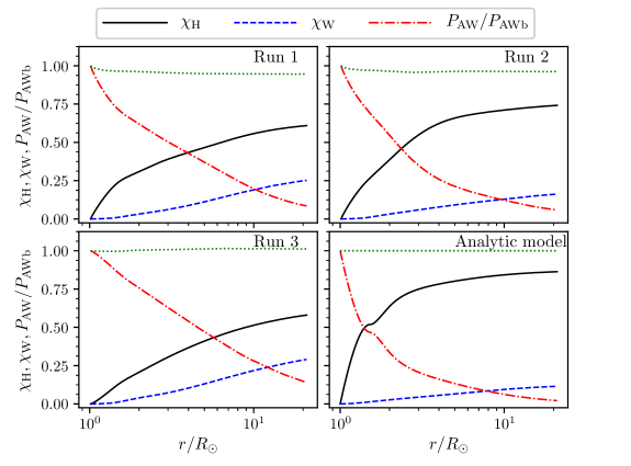
Figure 1: $\chi_{\rm H}(r)$ (solid) and $\chi_{\rm W}(r)$ (dashed) are the fractions of the Sun’s AW power injected at the base that are transferred to solar-wind particles via heating and work, respectively, between the coronal base and heliocentric distance $r$. $P_{\rm AW}/P_{\rm AWb}$ (dashed-dotted) is the fraction of the power that remains at each heliocentric distance $r$. These fractions are evaluated for Run 1, Run 2, and Run 3 using the expressions in Section 2.1 and for the CH09 analytic model (lower-right panel) using the expressions in Section 3.2. All four panels are computed using the $n(r)$, $B_{0}(r)$, and $U(r)$ profiles in (23) through (25). The green dotted lines represent the sum of the three fractions, which due to energy conservation equal one in steady state. Small deviations from one in the numerical simulations are due primarily to averaging over a finite number of realizations rather than a full ensemble representing a true statistical state.

3.3 The fractions of the AW power that are converted into heat and work

Figure 1 shows the fractions $\chi_{\rm H},\chi_{\rm W}$ and $P_{\rm AW}/P_{\rm AWb}$ for Run 1, Run 2 and Run 3, as well as the corresponding fractions calculated from the analytic model described in the previous section, using equations (23), (24), (25), (38), (39), (40), and the numerical values of relevant parameters listed in table 2. In the simulations, the heating fractions are calculated using equations (9), (10), (11), (13), (18) and (19). Assuming ergodicity in space and time at each radius, ensemble averages in equations (9), (11) and (13) are computed using a combined average over time (during the simulation’s steady state) and over the cross-sectional area of the fluxtube. More precisely, ensemble averages of any quantity $f=f(\mathbf{x},t)$ in the simulations are computed as

$$\left\langle f\right\rangle\equiv\frac{1}{T}\int_{0}^{T}\left(\frac{1}{a}\int_{S}fda\right)dt,$$ (41)

where $S$ is the cross-sectional surface of the fluxtube at each radius.

The reason that $\chi_{\rm H}(r_{\rm A})$ is greater than 0.5 in the simulations is that a moderate fraction of the remaining AW energy flux dissipates each time the outward-propagating AWs pass through one Alfvén-speed scale height (Dmitruk et al., 2002; Chandran & Hollweg, 2009), and there are a few Alfvén-speed scale heights between $r=r_{\rm b}$ and $r=r_{\rm A}$. On the other hand, the work fraction $\chi_{\rm W}\lesssim 0.3$ is significantly smaller because $v_{\rm A}>U$ at $r<r_{\rm A}$, and thus AWs at $r<r_{\rm A}$ are in an approximate sense speeding through a quasi-stationary background without doing much work. In contrast, at $r>r_{\rm A}$, $v_{\rm A}<U$, and the AWs can be thought of as being “stuck to the plasma,” which enhances the rate at which the fluctuations do work and causes work to become somewhat more efficient than heating. For example, $\chi_{\rm W}(21R_{\odot})-\chi_{\rm W}(r_{\rm A})$ equals 0.05, 0.027, 0.062, and 0.017 in Run 1, Run 2, Run 3, and the analytic model, respectively, whereas $\chi_{\rm H}(21R_{\odot})-\chi_{\rm H}(r_{\rm A})$ equals 0.04, 0.026, 0.055, and 0.016 in Run 1, Run 2, Run 3, and the analytic model, respectively. Although work is slightly more efficient than heating at transferring energy from AWs to solar-wind particles between $r=r_{\rm A}$ and $r=21R_{\odot}$, most of the AW energy flux has dissipated by the time the AWs reach $r_{\rm A}$, and the amount of AW power that is transferred to particles via work in this region is only a tiny fraction ($\lesssim 6\%$) of $P_{\rm AWb}$.

The different efficiencies of AW energy loss via work inside and outside the Alfvén critical point are in some ways analogous to the different rates at which energetic particles lose energy in the expanding solar wind in the scatter-free and scatter-dominated regimes (Ruffolo, 1995). When pitch-angle scattering is weak, energetic particles race through the plasma, their energies are approximately conserved, and they do negligible work on the plasma. In contrast, when pitch-angle scattering is strong, energetic particles are “stuck to the plasma,” and they lose energy through adiabatic expansion, because the scattering centers that “collide” with the particles are rooted in the plasma and diverge from one another as the plasma expands. As the particles lose energy, they do work on the background flow.

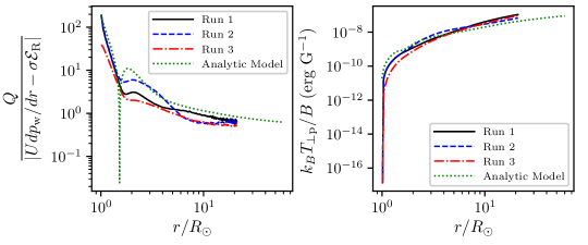
Figure 2: Left panel: The ratio of the heating rate $Q$ to the rate at which AWs do work on the flow per unit volume, $|U\textrm{d}p_{\rm w}/\textrm{d}r-\sigma\mathcal{E}_{\rm R}|$, as a function of heliocentric distance $r$. Heating is much more efficient than work close to the Sun, but at $r>r_{\rm A}=11.1R_{\odot}$, work becomes slightly more efficient than heating. Right panel: The average proton magnetic moment, $k_{\rm B}T_{\perp\rm p}/B$, as a function of heliocentric distance $r$, computed using (29), (30), (31), (43), (23), (24), and (25), with $f_{\perp\rm p}=0.9$, $z^{+}_{\rm rms,b}=72\mbox{ km}\mbox{ s}^{-1}$, and $T_{\perp\rm pb}=10^{6}\mbox{ K}$.

In the left panel of Figure 2, we plot the ratio of $Q$ to $|U\textrm{d}p_{\rm W}/\textrm{d}r-\sigma U{\mathcal{E}}_{\rm R}|$. These two quantities are the rates of heating and work per unit volume, which appear on the right-hand side of (16). This figure further illustrates the increasing relative efficiency of work beyond the Alfvén critical point, where the AWs become less mobile. The sharp feature in $Q/|U\textrm{d}p_{\rm W}/\textrm{d}r-\sigma U{\mathcal{E}}_{\rm R}|$ at $r=r_{\rm m}=1.72R_{\odot}$ in the analytic model (in which ${\cal E}_{\rm R}$ is taken to be negligible in comparison to $p_{\rm W}$) is an artifact of the local nature of the CH09 model, in which $z^{-}_{\rm rms}$ is determined at each $r$ by balancing the local rate of wave reflection against the local rate at which $\bm{z}^{-}$ fluctuations cascade and dissipate. This local balance causes $z^{-}_{\rm rms}$ and $Q$ to be proportional to $|\textrm{d}v_{\rm A}/\textrm{d}r|$, which vanishes at $r=r_{\rm m}$. In our numerical simulations, $\bm{z}^{-}$ fluctuations propagate some radial distance before dissipating, and $z^{-}_{\rm rms}$ and $Q$ remain nonzero at $r=r_{\rm m}$, as seen in the $Q$ profiles for numerical simulations shown in figure 2.

3.4 Magnetic-moment production

Beyond the sonic point at $r=r_{\rm s}$ ($r_{\rm s}\simeq 2R_{\odot}$ in coronal holes), the solar-wind outflow velocity exceeds the proton thermal speed $v_{\rm Tp}$, and the expansion time scale $r/U$ becomes shorter than the minimum time in which heat can conduct over a distance $r$, which is $\sim r/v_{\rm Tp}$. Proton thermal conduction can thus be neglected to a reasonable approximation at $r>r_{\rm s}$. For simplicity, in this section, we neglect proton thermal conduction at all $r$. We also neglect energy transfer from proton-electron collisions, as well as temperature isotropization from collisions and instabilities. The rate at which the average proton magnetic moment $k_{\rm B}T_{\perp\rm p}/B$ increases with $r$ is then given by (Sharma et al., 2006; Chandran et al., 2011)

$$BnU\frac{\mathrm{d}}{\mathrm{d}r}\left(\frac{k_{\rm B}T_{\perp\rm p}}{B}\right)=f_{\perp\rm p}Q,$$ (42)

where $k_{\rm B}$ is the Boltzmann constant, $T_{\perp\rm p}$ is the perpendicular proton temperature, and $f_{\perp\rm p}(r)$ is the fraction of the heating rate that goes into perpendicular proton heating at heliocentric distance $r$. We approximate (42) by setting $B(r)=B_{0}(r)$. Upon dividing (42) by $B_{0}nU$, integrating, and making use of (34), we obtain

$$\frac{k_{\rm B}T_{\perp\rm p}}{B_{0}}=\frac{k_{\rm B}T_{\perp\rm pb}}{B_{0b}}+\int_{\rm r_{\rm b}}^{r}\frac{f_{\perp\rm p}(r^{\prime})Q(r^{\prime})B_{0\rm b}}{n_{\rm b}U_{\rm b}[B_{0}(r^{\prime})]^{2}}\textrm{d}r^{\prime}.$$ (43)

The form of the integrand in (43) shows that a given amount of heating produces more magnetic moment in regions of weaker magnetic field.

In right panel of figure 2, we plot the average magnetic moment $k_{\rm B}T_{\perp\rm p}/B$ as a function of $r$ using (23), (24), (25), (29), (30), (31), and (43), with $f_{\perp\rm p}=0.9$, $z^{+}_{\rm rms,b}=72\mbox{ km}\mbox{s}^{-1}$, and $T_{\perp\rm pb}=10^{6}\mbox{ K}$. Figures 1 and 2 show that, although only a small fraction of $P_{\rm AWb}$ is dissipated at $r>r_{\rm A}$, $k_{\rm B}T_{\perp\rm p}/B$ rises robustly at $r>r_{\rm A}$.

4 Conclusion

In this paper, we use direct numerical simulations of RDAWT to determine $\chi_{\rm H}(r)$ and $\chi_{\rm W}(r)$, the fractions of the AW power at the coronal base ($P_{\rm AWb}$) that are transferred to the solar wind via heating and work between the coronal base ($r=r_{\rm b}$) and radius $r$. Our simulations solve for the evolution of transverse, non-compressive fluctuations in a fixed background solar wind whose density, magnetic-field strength, and outflow-velocity profiles are chosen to emulate a fast-solar-wind stream emanating from a coronal hole. We find that heating from the cascade and dissipation of AW fluctuations between $r_{\rm b}$ and the Alfvén critical point $r_{\rm A}$ transfers between 50% and 70% of $P_{\rm AWb}$ to the solar wind, whereas work in this same region transfers between 15% and 30% of $P_{\rm AWb}$ to the solar wind. The variation in these numbers arises from the different photospheric boundary conditions imposed in our different numerical simulations.

The reason that $\chi_{\rm H}(r_{\rm A})$ is in the range of 50% to 70% is that a moderate fraction of the local AW power dissipates within each Alfvén speed scale height (Dmitruk et al., 2002; Chandran & Hollweg, 2009), and there are a few Alfvén speed scale heights between $r_{\rm b}$ and $r_{\rm A}$. The reason that $\chi_{\rm W}(r_{\rm A})$ is small compared to 1 is that $v_{\rm A}>U$ at $r<r_{\rm A}$, so AWs in this sub-Alfvénic region are in an approximate sense speeding through a quasi-stationary background without doing much work. Work becomes relatively more efficient at transferring AW energy to the particles at $r>r_{\rm A}$, where $v_{\rm A}<U$ and the AWs are in an approximate sense “stuck to the plasma.” However, because most of the Sun’s AW power dissipates via heating before the AWs reach $r_{\rm A}$, the total rate at which work transfers AW energy to the plasma at $r>r_{\rm A}$ is a small fraction of $P_{\rm AWb}$. Although only a small fraction of $P_{\rm AWb}$ survives to reach $r_{\rm A}$, the average proton magnetic moment increases robustly at $r>r_{\rm A}$ (assuming that a substantial fraction of the turbulent heating rate goes into perpendicular proton heating at these radii), because heating becomes more effective at producing magnetic moment in regions of weaker magnetic field.

The accuracy of our results is limited by our neglect of compressive fluctuations, which enhance the dissipation of AW energy via “AW phase mixing” (Heyvaerts & Priest, 1983). Plasma compressibility further enhances the rate of AW dissipation via parametric decay (Galeev & Oraevskii, 1963; Sagdeev & Galeev, 1969; Cohen & Dewar, 1974; Goldstein, 1978; Spangler, 1986; Hollweg, 1994; Dorfman & Carter, 2016; Tenerani et al., 2017; Chandran, 2018). Three-dimensional compressible MHD simulations of the turbulent solar wind from $r=r_{\rm b}$ out to $r>r_{\rm A}$, such as those carried out by Shoda et al. (2019), could lead to improved estimates of $\chi_{\rm H}(r)$ and $\chi_{\rm W}(r)$.