Order-of-Magnitude Beam Current Improvement in Compact Cyclotrons

Abstract

There is great need for high intensity proton beams from compact particle accelerators in particle physics, medical isotope production, and materials- and energy-research. To address this need, we present, for the first time, a design for a compact isochronous cyclotron that will be able to deliver 10 mA of 60 MeV protons - an order of magnitude higher than on-market compact cyclotrons and a factor four higher than research machines. A key breakthrough is that vortex motion is incorporated in the design of a cyclotron, leading to clean extraction. Beam losses on the septa of the electrostatic extraction channels stay below 50 W (a factor four below the required safety limit), while maintaining good beam quality. We present a set of highly accurate particle-in-cell simulations, and an uncertainty quantification of select beam input parameters using machine learning, showing the robustness of the design. This design can be utilized for beams for experiments in particle and nuclear physics, materials science and medical physics as well as for industrial applications.

1 Introduction

This paper describes the design and simulations of a 10 mA, 60 MeV/amu compact cyclotron that can be mass-manufactured. Such a machine would have a transformative effect on multiple fields of fundamental and applied science, including neutrino physics, through the IsoDAR project [1, 2, 3]; isotope production for medicine and other uses [4, 5, 6]; materials testing for high radiation environments [7, 8, 9, 10, 11]; and as a pre-accelerator for a 10 mA, 800 MeV to 1 GeV cyclotron that can be used for Accelerator Driven Systems (ADS) [12, 13, 14, 15] and particle physics (e.g. the DAE$\delta$ALUS experiment [16, 17, 18, 19, 20]). We discuss these motivations below and summarize the applications in TAB. 1. This beam intensity is an order of magnitude higher than 60 to 100 MeV cyclotrons on the market [21, 22], and a factor of four higher than the Paul Scherrer Institute - Injector II cyclotron [23].

Figure 1: (From [24]) Schematic of the IsoDAR experiment at Kamioka. From left to right: The cyclotron (ion source on top), the medium energy beam transport line, the neutrino production target [25], and the KamLAND detector [26].

Table 1: A few potential uses for high current proton beams and how cyclotrons can be leveraged to reach the goals. ADSR: Accelerator Driven Sub-critical Reactors, ADS: Accelerator Driven Systems for nuclear waste transmutation. Cyclotrons can be a cost-effective alternative for tests and demonstrations at the low-power end of the spectrum (tens of mA).

Application	Current	Energy	Comment
IsoDAR [1, 2, 3]	10 mA	60 MeV	Use $\bar{\nu}_{e}$ from decay-at-rest to search for sterile neutrinos.
DAE$\delta$ALUS [16, 17, 18, 19, 20]	10 mA	800 MeV	A proposed search for leptonic CP violation.
ADSR [12, 13]	10-40 mA	$\sim 1$ GeV	Cost-effective alternative for demonstrator experiments.
ADS [14, 15]	4-120 mA	$\sim 1$ GeV	Cost-effective alternative for demonstrator experiments.
Isotopes [4, 5, 6]	$1-10$ mA	3-70 MeV	Produce more than 250 Ge/Ga generators per week [5].
Material tests [7, 8, 9, 10]	10-100 mA	5-40 MeV	Testing of fusion materials similar to IFMIF [11].

The cyclotron presented here was originally motivated by the need for high-flux sources of neutrinos for the precision study of transformation of neutrino flavor, or oscillations. This machine was proposed as the first in a two-cyclotron acceleration complex designed for the DAE$\delta$ALUS experiment, hence it is called the DAE$\delta$ALUS Injector Cyclotron or DIC. To address the DAE$\delta$ALUS goal of studying $CP$-violation in the neutrino sector [17], the complex must produce 10 mA of 800 MeV protons, which, when targeted, results in a well-understood neutrino flux from pion and muon decay-at-rest. Early on, it was recognized that the DIC also could be used stand-alone, to drive a novel electron anti-neutrino source arising from ⁸Li decay [1, 2, 3]. This concept, proposed as the Isotope Decay-At-Rest experiment (IsoDAR), targets 10 mA of protons at 60 MeV on beryllium to produce an intense neutron flux that bathes a ⁷Li target producing the required ⁸Li. The resulting $\beta^{+}$-decay-produced antineutrino flux allows for tests of $2\sigma$ to $4\sigma$ oscillation anomalies that are attributed to beyond Standard Model particles called “sterile neutrinos” [27]. IsoDAR can address the sterile neutrino hypothesis at the $>$5$\sigma$ level when the paired with a 1 kton neutrino detector. The proposed source design, which can be installed in the Kamioka mine in Japan, next to the KamLAND detector [26], is shown in FIG. 1. The “IsoDAR cyclotron” and the “DIC” are identical in design. For consistency, in this paper, we will use “IsoDAR cyclotron” throughout.

The energy of the IsoDAR cyclotron is similar to cyclotrons proposed for medical isotope production [4], but with an order of magnitude higher beam intensity. In particular a modestly-converted IsoDAR cyclotron can produce much-needed isotopes (²²⁵Ac and Ge/Ga generators) for medical treatment and imaging, as described in two recent publications [5, 6]. ⁶⁸Ge is the parent of the PET imaging isotope ⁶⁸Ga. ⁶⁸Ge has a 270 day half-life, making it ideal for storage and delivery, with the ⁶⁸Ga extracted at the hospital. One can envision dedicating 10% of the IsoDAR running time to production of ⁶⁸Ge. If, instead, a separate version of our cyclotron is constructed for dedicated isotope production, it can produce more than 250 Ge-Ga generators per week. ²²⁵Ac is a valuable alpha-emitter for cancer therapy. This new design can impinge 10 mA of protons on a natural thorium target to produce, in a dedicated machine, up to 20 doses per hour. This would substantially increase the world-wide production rate.

Another example is the use of compact cyclotrons to test materials proposed for use inside advanced nuclear reactors and fusion energy devices. Here, intense proton beams with energy of 10 to 30 MeV provide a platform to achieve relevant materials responses in a fraction of the time compared to conventional irradiation methods inside nuclear reactors [9, 7]. The small footprint and relatively moderate costs makes them attractive for university laboratories, facilitating student involvement and interdisciplinary research [10].

Among the IsoDAR cyclotron challenges are the strong space charge effects of such a high-intensity beam and the small phase acceptance window of an isochronous cyclotron, accelerating protons. Space charge, the mutual Coulomb repulsion of the beam particles inside each bunch, matters most in the Low Energy Beam Transport line (LEBT) and during injection into the cyclotron. It leads to beam growth and, ultimately, particle loss when the bunch dimensions exceed the physical constraints of the accelerator. Phase acceptance poses a similar problem, where particles entering the cyclotron at the wrong phase, with respect to the RF cavities’ oscillating voltage, will gain too little or too much energy and consequently go on unfavorable trajectories. This leads to energy spread and halo formation. Both effects cause overlapping final turns and high particle loss during extraction, which leads to excess thermal load and activation of the hardware.

To overcome these challenges, the IsoDAR cyclotron concept is based on three innovations:

1. Accelerating 5 mA of $\mathrm{H}_{2}^{+}$ instead of 10 mA of protons leads to the same number of nucleons on target at half the electrical current, as the remaining electron bound in the $\mathrm{H}_{2}^{+}$ molecular ion reduces the electrical current in the beam by 50 %.

2. Injecting into the compact cyclotron via a Radio-Frequency Quadrupole (RFQ) partially embedded in the yoke aggressively pre-bunches the beam significantly increasing the acceptance.

3. Designing the cyclotron main acceleration to optimally utilize vortex motion leads to clean extraction. This effect can stabilize beam growth and is explained in Section 3.

The focus of this publication lies on the simulation of the main acceleration, from turn 2 (194 keV/amu) to turn 103 (60 MeV/amu), and the demonstration of the IsoDAR cyclotron design’s capability to use vortex motion to keep a stable, round longitudinal-radial bunch shape all the way to the final turn and thus accelerate 5 mA of $\mathrm{H}_{2}^{+}$ while keeping the beam losses in the extraction region around 50 W. An upper limit of 200 W for hands-on maintenance corresponds to relative losses on the order of 10^-4 and is based on practical experience at the Paul-Scherrer-Institute Injector II cyclotron [28]. The robustness of the design and simulations is then shown by means of an uncertainty quantification using machine learning techniques.

In the following section, we review the latest IsoDAR cyclotron design. To give a more complete picture, we also briefly describe the current design status of the injection system, including ion source, RFQ, and central region, although the particle distributions resulting from injection system simulations have not yet been used in the main acceleration simulations. Methodology and simulation strategies are discussed in Section 3. Our simulations in Section 4 demonstrate that fully acceptable beam can be delivered to the extraction system, by careful collimator placement, even if the beam is not perfectly matched at injection. Inclusion of the injection system to close the full start-to-end chain will likely require retuning of the collimators, but not change our findings. Finally, Uncertainty Quantification (UQ) using Machine Learning (ML) will be shown in Section 5.

2 Hardware Considerations

Figure 2: Schematic of the IsoDAR cyclotron. Indicated are the hills (magenta) and valleys (yellow) of the isochronous field, the four double-gap RF cavities (centered around 45^∘, 135^∘, 225^∘, and 315^∘), the 60 MeV/amu static equilibrium orbit, and examples of deflectors and magnetic channels (MC1 and MC2). The outer diameter is 6.2 m. From [29].

This publication focuses on the design, simulation, and uncertainty quantification of the IsoDAR 60 MeV/amu cyclotron, using, for the first time, vortex-motion in the design process. The IsoDAR cyclotron magnet and RF cavities will be described in the following subsection. The starting point of the simulation study is a particle bunch with an average kinetic energy of 193 keV/amu, placed in the first turn. Because the injection of a high-current beam into a compact cyclotron requires care, significant work has also been done on the injection system, comprising an $\mathrm{H}_{2}^{+}$ ion source, an RFQ buncher-accelerator, embedded axially in the cyclotron yoke, and the central region of the cyclotron with a spiral inflector. This RFQ is operated at the cyclotron RF frequency of 32.8 MHz. A proof-of-concept machine is currently being constructed to experimentally demonstrate the capability to inject and match the needed $\mathrm{H}_{2}^{+}$ beam current into the cyclotron: The RFQ-Direct Injection Project (RFQ-DIP) [30, 31]. For completeness, we briefly describe RFQ-DIP and central region in subsections 2.2 and 2.3, respectively, but it should be stressed that this work is ongoing and a separate publication on injection is forthcoming.

2.1 Cyclotron Magnet and RF Design

Table 2: Parameters of the IsoDAR cylclotron. Power/cavity assumes a 50% efficiency at transferring RF power to the beam.

Parameter	Value	Parameter	Value
$E_{max}$	60 MeV/amu	$E_{inj}$	35 keV/amu
$R_{ext}$	1.99 m	$R_{inj}$	55 mm
$\langle B\rangle$ @ $R_{ext}$	1.16 T	$\langle B\rangle$ @ $R_{inj}$	0.97 T
Sectors	4	Hill width	25.5 - 36.5 deg
Valley gap	1800 mm	Pole gap	80 - 100 mm
Outer Dia.	6.2 m	Full height	2.7 m
Cavities	4	Cavity type	$\lambda/2$, 2-gap
Harmonic	4th	rf frequency	32.8 MHz
Acc. Voltage	70 - 240 kV	Power/cavity	$310$ kW
Coil size	200x250 mm2	Current dens.	3.167 A/mm2
Iron weight	450 tons	Vacuum	$<10^{-7}$ mbar

The IsoDAR cyclotron is a compact isochronous cyclotron operating at 32.8 MHz (4^th harmonic of the particle revolution frequency 8.2 MHz). The design has been presented in detail elsewhere [29, 32, 3, 19] and will be reviewed here. A schematic of the machine is shown in FIG. 2 and important parameters are listed in TAB. 2.

Figure 3: RF cavity modelled in the multiphysics software CST [33]. The colors correspond to surface current density. Central stems are used for support and frequency tuning. The cavities are made from oxygen-free high-conductivity (OFHC) copper. From [3].

Being a compact cyclotron, the main magnetic field is produced by a single pair of coils encompassing the entire machine and a shared return yoke for the four sectors. Notably, the hill gap is large at 100 mm (except for the center, where it is reduced to 80 mm to increase vertical focusing) to allow for a large vertical beam size. Furthermore, the magnet design includes a $\nu_{r}=1$ resonance crossing close to extraction, which leads to precessional motion and improved turn separation. This is achieved by shaping the magnet poles at larger radii accordingly. To increase azimuthal field variation (flutter), and thus vertical focusing in the first turn, a vanadium-permendur (VP) insert is envisioned on the inner pole tips (see FIG. 5). The magnet was designed using the Finite Elements Analysis software OPERA [34] and the generated field was exported for the simulations.

As was shown by Joho [35], a high energy gain per turn is crucial to acceleration of a high current beam. In the IsoDAR cyclotron, we place four $\lambda/2$ double-gap RF cavities in the four magnet valleys. Their design is based on that of commercial cyclotrons and they are tuned for 4^th harmonic operation. These RF cavities have a radial voltage distribution going from 70 kV at the injection radius to 240 kV at extraction. With a synchronous phase $\Phi_{S}=-2.5^{\circ}$ (close to the crest), this amounts to energy gains per turn between 500 keV and 2 MeV during the acceleration process. The cavity is shown in FIG. 3. The radial voltage distribution calculated in the multiphysics software CST [33] is used in the simulations for each of the eight acceleration gaps.

2.2 The RFQ-Direct Injection Project

Figure 4: Schematic of the IsoDAR cyclotron (left) next to the RFQ Direct Injection Prototype (right). Ions are produced in the ion source (top), are accelerated and bunched in the RFQ (middle) and injected into the cyclotron central region to be accelerated.

RFQ-DIP [30, 31] is the prototype of a novel injection system for compact cyclotrons. A cartoon of the device is shown in FIG. 4. RFQ-DIP comprises a multicusp ion source (MIST-1) [36, 24], a short matching LEBT with chopping and steering capabilities, and an RFQ that is embedded in the cyclotron yoke, to axially inject a highly bunched beam into the central region through a spiral inflector. By aggressively pre-bunching the beam, we fit more particles into the RF phase acceptance window of $\approx 20^{\circ}$. The system is designed to produce and inject up to 15 mA of $\mathrm{H}_{2}^{+}$. Early commissioning runs with MIST-1 have shown a 76 % $\mathrm{H}_{2}^{+}$ fraction at 11 mA/cm² and a maximum current density of 40 mA/cm² when the source is tuned for $\mathrm{H}_{3}^{+}$ [24]. This is currently a factor 4 short of the design goal. However, further upgrades to cooling and extraction system are ongoing that we anticipate will yield the necessary beam currents. In Ref. [31], we also describe the physics design of the RFQ linear accelerator-buncher that will be embedded in the cyclotron yoke. It will deliver a highly bunched beam to the spiral inflector – an electrostatic device that bends the beam from the axial direction into the acceleration plane of the cyclotron (median plane, or mid-plane), where the beam is accelerated and matched to the cyclotron main acceleration (described in Section 4). Due to the high bunching factor and strong space charge, the beam starts diverging in transverse direction and de-bunching in a longitudinal direction soon after the RFQ exit. To mitigate this, we included a re-bunching cell in the RFQ design and place an electrostatic quadrupole focusing element before the spiral inflector. Furthermore, the spiral inflector electrodes can be carefully shaped to add vertical focusing. First simulations of the full injector (up to the exit of the spiral inflector) showed transmission of $\approx 78\%$ for two test cases (10 mA and 20 mA of total beam current, 80% $\mathrm{H}_{2}^{+}$, 20% protons) with transverse emittances of $0.3-0.4$ mm-mrad (RMS, normalized) and longitudinal emittances of $7-8$ keV/amu-ns (RMS) [31].

2.3 Central region

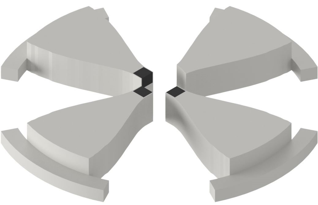
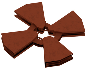
Figure 5: CAD renderings of the central region. Left: The iron poles for magnetic field calculations (lower half only). The VP inserts can be seen in black at the pole tips. One of the pole tips is truncated, yielding space for the spiral inflector. Right: The RF electrodes with tips angled to adjust the phase during the first two turns.

In parallel with the simulation study presented in this manuscript, and complementary to it (overlapping in the first four turns of the cyclotron), a detailed central region study, subcontracted to the company AIMA Developpement in France, was performed, and summarized in a technical report [37]. In this study, a 3D magnetic field was generated that includes the effects of VP inserts in the pole tips, and mimics the center field of the IsoDAR cyclotron. One pole tip was cut short to make room for the spiral inflector (see FIG. 5 (left)). The VP has a sharper turn in the B-H curve, slightly improving the flutter in the central region. An optimized dee electrode system was generated, which can be seen in FIG. 5 (right). This system exhibits good vertical focusing and small orbit center precession. The dee peak voltage was increased to 80 kV from the nominal 70 kV in the IsoDAR baseline, which is high, but achievable. Particle distributions from a simulation of the ion source extraction and RFQ injector (described in the previous section) were used as initial conditions in the AIMA study.

Figure 6: Left: Trajectories of the first 3.5 turns (2 MeV) in the simulated central region. Right: Demonstrated turn separation of 1 cm (edge-to-edge) after placing a single collimator in the first turn. Beam transmission from the entrance of the spiral inflector to the probe was 42%. From [37].

The desired edge-to-edge turn separation of 10 mm in the fourth turn (at 1 MeV/amu beam energy) was achieved by placing a single collimator in the first turn (see FIG. 6). The combined beam loss in the spiral inflector and in the central region (mostly on the single collimator) was 58% and thus the cumulative transmission efficiency was 42% from ion source to turn 4 of the cyclotron. Should we take these results at face value, a total current of 20 mA (comprised of 80 % $\mathrm{H}_{2}^{+}$ and 20 % protons) would be needed from the ion source and injected into the RFQ. In Ref. [31] we showed that the RFQ-DIP system can handle such a current. However, this central region study, as of yet, does not include space charge effects (space charge was included only up to the entrance of the spiral inflector, cf. previous section). As we will show in Section 4, including space-charge will, somewhat counter-intuitively, improve the situation, as the vortex-effect will help maintain a stable distribution and only halo particles will have to be removed with collimators. Furthermore, placement of several collimators instead of one allows more control over which particles are removed, yielding lower losses. This does not hold for the spiral inflector itself, where including space charge will lead to slightly lower transmission. Future work will combine the results presented in Section 4 with the design work performed in the AIMA study, by importing the 3D magnetic and electric fields of the CAD model into OPAL and tracking with space charge, using the cyclotron injection mode described in Ref [38].

3 Methodology

3.1 OPAL simulation code

OPAL [39] is a suite of software for the simulation of particle accelerators, which originates at the Paul Scherrer Institute, and which is programmed in C++. One of the available flavors is OPAL-cycl, which is specifically created to simulate cyclotrons, and which we used for this study. The following is a brief summary of the description in [38]. OPAL uses the Particle-In-Cell (PIC) method to solve the collisionless Vlasov equation

$$\frac{df}{dt}=\partial_{t}f+\sum_{j=1}^{M}\left[\frac{\partial f}{\partial\mathbf{x}_{j}}\dot{\mathbf{x}}_{j}+q(\mathbf{E}+c\mbox{\boldmath$\beta$}\times\mathbf{B})_{j}\frac{\partial f}{\partial\mathbf{P}_{j}}\right],$$

in the presence of external electromagnetic fields and self-fields,

$$\mathbf{E} = \mathbf{E}_{\mathrm{ext}}+\mathbf{E}_{\mathrm{self}},$$ (1)

$$\mathbf{B} = \mathbf{B}_{\mathrm{ext}}+\mathbf{B}_{\mathrm{self}}.$$ (2)

Here, $\mathbf{x}$ and $\mathbf{P}$ are the canonical position and momentum of the particles in the distribution function

$$f(\mathbf{x},\mathbf{P},t):(\Re^{3M}\times\Re^{3M}\times\Re)\rightarrow\Re,$$

and $M$, $c$, $t$, $q$, and $\mbox{\boldmath$\beta$}=\mathbf{v}/c$, the number of simulation particles, vacuum speed of light, time, charge of a particle, and velocity scaled by c, respectively. A 4^th order Runge-Kutta (RK) integrator is used for time integration. External fields are evaluated four times per time step. Self-fields are assumed to be constant during one time step, because they typically vary much slower than the external fields.

The self fields $\mathbf{E}_{\mathrm{self}}$ and $\mathbf{B}_{\mathrm{self}}$ are calculated on a grid using a Fast Fourier Transform (FFT) method. The external fields $\mathbf{E}_{\mathrm{ext}}$ and $\mathbf{B}_{\mathrm{ext}}$ can be calculated with any method of the users choosing and then loaded into OPAL either as a 2D median plane field (magnetic field only) or a full 3D electromagnetic field map. OPAL uses a series expansion to calculate off-plane elements from the 2D median plane fields. Furthermore, the 3D maps are time-varied according to

$$\mathbf{E}_{\mathrm{ext,3D}}(t)=\mathbf{E}_{\mathrm{ext,3D,0}}\cdot\cos(\omega_{\mathrm{RF}}t-\phi_{S})$$

with $\omega_{\mathrm{RF}}$ the cyclotron RF frequency and $\phi_{S}$ the phase. If a static 3D field is desired, the frequency and phase can be set to zero. Here, we used OPERA to calculate the median plane field and COMSOL [40] for the 3D electrostatic fields of the extraction system.

OPAL-cycl comes with a number of built-in diagnostic devices. One such diagnostic is the OPAL PROBE. It is a 2D rectangle placed in the 3D simulation space. Whenever a particle crosses the probe plane, it is registered and the particle data is added to the probe data storage. In Section 4 we denote probes with a single line in a top-down view of the cyclotron. Trajectory data, probe data, and data of particles lost on collimators are stored by OPAL in separate files in HDF5 [41] data format. All post-processing is done in Python 3.7 [42].

OPAL has been extensively tested and benchmarked. Pertaining to the cyclotron studies presented here, we cite three examples:

OPAL was used to study beam dynamics in PSI Injector II, where high-fidelity simulations of the full cyclotron using $10^{6}$ particles were performed that showed the formation of a stable vortex [43] (cf. Subsection 3.3). In [43], the effects of radially neighboring bunches in the PSI ring cyclotron were also investigated. A comparison of OPAL simulations with radial probe measurements in Injector II, yielding good agreement, was shown in [28, Fig. 3]. More recently, a detailed study was performed for the planned 3 mA upgrade of PSI Injector II that further corroborates the fidelity of the code and the applicability of the vortex motion design concept for high intensity cyclotrons [44].

3.2 Coordinate systems

Trajectory data and general layout images are shown in the laboratory frame (global coordinates). However, as vortex motion happens through coupling in the longitudinal-radial plane and collimators can only scrape particles that extend away from the bunch in the direction perpendicular to the direction of bunch movement (mean momentum), it is convenient to look at the bunch in a local frame (local coordinates) that are defined as follows: vertical: $\tilde{\mathrm{z}}$ = z, longitudinal: $\tilde{\mathrm{y}}$ = direction of mean bunch momentum, transversal (also called “radial” here): $\tilde{\mathrm{x}}$ = orthogonal to $\tilde{\mathrm{z}}$ and $\tilde{\mathrm{y}}$. N.B.: The radial direction does not necessarily coincide with the ray originating in the origin and passing through the bunch center, as the magnetic field is not uniform, but has hills and valleys.

3.3 Vortex-motion

Figure 7: An intuitive picture of vortex motion. The beam is presented in its local frame (cf. text) and the direction of the additional velocity component $\mathbf{v}_{E}$ due to an $\mathbf{E}\times\mathbf{B}$ drift is indicated for the four extrema of the bunch. Inspired by [45].

Figure 8: OPAL-cycl simulation of a single, coasting bunch in PSI injector II, shown in its local frame, moving to the left. Beam current: 1 mA, beam energy: 60 MeV. Left to right: Upper row: turn 0, 5, 10, lower row: turn 20, 30, 40. From [43].

In isochronous cyclotrons, the interaction between the self fields of the beam, arising from space charge, and the external magnetic forces, from the cyclotron main magnet, can lead to the formation of a stable, almost round, spatial distribution in the horizontal plane. In this subsection, we give a brief overview on the current understanding of this effect, dubbed vortex motion.

Vortex motion was first seen in PSI Injector II, and subsequently investigated and confirmed both experimentally and through computer simulations [46, 47, 48]. A simplified, but intuitive picture inspired by Ref [45] is shown schematically in FIG. 7. Here, only the force at the four extrema (longitudinal and radial minima and maxima) of the bunch in the local frame ($\tilde{\mathrm{x}}$, $\tilde{\mathrm{y}}$, $\tilde{\mathrm{z}}$) are considered. This is simply the Lorentz force due to self fields and external fields:

$$\mathbf{F}=q\cdot(\mathbf{v}\times\mathbf{B}_{\mathrm{ext}})+q\cdot\mathbf{E}_{\mathrm{self}}$$

with $\mathbf{B}_{\mathrm{ext}}=\mathbf{e}_{\tilde{\mathrm{z}}}B_{0}$. Here $\mathbf{e}_{\tilde{\mathrm{x}}}$, $\mathbf{e}_{\tilde{\mathrm{y}}}$, and $\mathbf{e}_{\tilde{\mathrm{z}}}$ are the coordinate vectors of the local frame. Neglecting for a moment the self term, the solution to the equation of motion would be the usual circular motion of the particles in the magnetic dipole field. Assuming mid-plane symmetry, $E_{\tilde{\mathrm{z}}}$ must be zero, and the addition of the self term leads to an $\mathbf{E}\times\mathbf{B}$ drift in the $\tilde{\mathrm{x}}$-$\tilde{\mathrm{y}}$ plane that adds an additional velocity term to each particle:

$$\mathbf{v}_{E}=\frac{\mathbf{E}_{\mathrm{self}}\times\mathbf{B}_{\mathrm{ext}}}{\mathrm{B_{\mathrm{ext}}}^{2}}.$$

For example, at the head of the bunch (P₁ in FIG. 7), $\mathbf{E}_{\mathrm{self}}=\mathbf{e}_{\tilde{\mathrm{x}}}E_{\tilde{\mathrm{x}}}$ and consequently, $\mathbf{v}_{E}=\mathbf{e}_{\tilde{\mathrm{y}}}\cdot(E_{\tilde{\mathrm{x}}}B_{0})/\mathrm{B}^{2}$. Similar relations hold for P₂, P₃, and P₄ and lead to the velocity vectors indicated in FIG. 7, which in turn lead to the spiraling motion in the local frame. A simulation of this effect in PSI Injector II is shown in FIG. 8. In reality, the situation is, of course, more complex, as the magnetic field is not uniform but an Azimuthally Varying Field (AVF) and the space charge force is not linear, as was assumed in the intuitive picture.

An early theoretical approach to vortex motion was presented in [49]. A more rigorous treatment for AVF cyclotrons was presented in [50] and later extended to the central region and injection in [51]. These methods allow finding matched distributions under the assumption that the energy gain per turn is small compared to the beam energy (adiabatic energy gain). These theories together with simulations and experimental studies suggest that, in order for the beam to be well matched, a very short bunch with minimal energy spread should be injected into the cyclotron at high energy. In practice, this is not possible in a compact cyclotron with axial injection, as the spiral inflector typically can only hold voltages $<20$ kV without sparking, due to space restrictions. As described at the end of [51], in the center of the cyclotron, where energy gain cannot be adiabatic by the nature of the machine, a careful collimation process must then be employed to shape the bunch in longitudinal-radial phase space. This is what we have done here and what is described in Subsection 9. At higher energies (main acceleration), the stable distribution has then formed and all the points of [50] hold, which means that very high current beams can be accelerated, albeit with significant losses on the central region collimators to cut away halo until the stable round distribution has formed.

3.4 Collimator modelling

Figure 9: Calculation of the 3D electrostatic septum field in three steps: Left: Calculation of the coordinates in Python with visual feedback. Center: Export into a Autodesk Inventor macro to generate the 3D CAD model. Right: Import into COMSOL and calculation of the field.

Collimators are placed in the OPAL-cycl code as CCOLLIMATOR objects in the input scripts using the following syntax [52]:

    "Name": CCOLLIMATOR, WIDTH=w
            XSTART=x1, XEND=x2,
            YSTART=y1, YEND=y2,
            ZSTART=z1, ZEND=z2;

where “Name” is a unique label for the collimator, x1, x2, y1, y2 are the start and end coordinates along the direction of movement, w is the width of a single collimator block perpendicular to the direction of movement (both in the cyclotron median plane), and z1, z2 mark the vertical extent. OPAL terminates particles intersecting with collimators and saves the particle data of lost particles in an HDF5 file.

The manual optimization of collimator placement is an iterative process consisting of the following steps:

1. The beam is tracked for ten turns while saving the full 6D particle distributions 250 times per turn (2500 data-sets).

2. Particle distributions at each step are projected onto the median plane and transformed into their local frame.

3. Good positions (time steps) to scrape halo particles are manually selected, length, width and height are specified by the user, and a Python script is used to generate the text to add the new collimators to the OPAL input file.

4. Return to Step 1: The simulation is run again with the new collimator(s).

5. Occasionally, all 103 turns are simulated while saving particles only 4 times per turn and the data on the probes is analyzed to see what the anticipated beam loss on the septum will be.

The placement of collimators used in Section 4 (cf. FIG. 11) is optimized by hand, following the process described above. Using the surrogate modelling described in Section 5, an optimization of the radial collimator positions was performed that yielded no significant improvement, showing that the solution is robust.

3.5 Extraction Channel Modelling

The electrostatic extraction septa (grounded) and corresponding puller electrodes (at negative high voltage potential) are generated in an iterative process. In each iteration, the same workflow is used to obtain a 3D electrostatic field map for OPAL. We limit our description to the process for Septum 1 with the understanding that, with the exception of the azimuthal position of the septum, it is identical to that for Septum 2. The workflow in each iteration comprises the following steps (see also FIG. 9):

1. Numerical calculation of septum position using Python. The Python script creates a text file with the coordinates of the septum strips. OPAL-cycl uses these coordinates to place CCOLLIMATOR objects. It also generates a Visual Basic macro to automatically generate the 3D model in Inventor.

2. Generation of a 3D CAD model of the septum and puller electrodes in Autodesk Inventor [53]. The macro from Step 1 is used.

3. Import of the Inventor model into COMSOL [40] and calculation of the electrostatic fields. A mesh refinement study was performed to determine the correct mesh size, which was then kept throughout the process.

4. Import of the 3D field into OPAL-cycl as a static field map. This is achieved by loading it as an RF-field map with $\omega_{\mathrm{RF}}$ set to zero.

In the first iteration, a baseline high-fidelity OPAL simulation without septa is used for the placement of a septum that has twice the nominal gap width and twice the nominal voltage (thus keeping the electric field strength the same, while giving the beam space to move radially outwards as intended). In the second iteration, the new trajectories are used to place the septum and puller electrodes, now with nominal width and voltage, symmetrically around the beam in their final position. This process is then repeated for the second septum-puller pair.

4 Beam Dynamics Simulations in the IsoDAR cyclotron

A preliminary study of the IsoDAR cyclotron was performed in [54] with encouraging results. Since then, the harmonic was changed from 6 to 4 and the mean starting energy was reduced from 1.5 MeV/amu to 194 keV/amu. This is a change in starting position from the fourth turn down to the first turn. More careful collimator placement and a full 3D treatment of the electrostatic septa were added to the simulations to demonstrate the capability of accelerating and extracting 5 mA of $\mathrm{H}_{2}^{+}$.

Figure 10: Beam projections onto the median plane in local frame. (a) Turn 0, initial beam, (b) Turn 6, no space charge. (c) Turn 6, $\mathrm{I}_{\mathrm{beam}}=6.65$ mA, no collimators, (d) Turn 6, $\mathrm{I}_{\mathrm{beam}}=6.65$ mA, 12 collimators The development of a round $\tilde{\mathrm{x}}$-$\tilde{\mathrm{y}}$ distribution can be seen after six turns when space charge is present (c, d). Halo that is formed in the process can be removed with collimators (d).

4.1 First Turns and Collimation

Table 3: Initial bunch parameters in the local frame.

Parameter	Value	Parameter	Value
Distr. type	Gaussian	Ekin,mean	194 keV/amu
$\sigma_{\tilde{\mathrm{x}}}$	1 mm	$\tilde{\mathrm{x}}$-cutoff	$4\sigma$
$\sigma_{\tilde{\mathrm{y}}}$	3 mm	$\tilde{\mathrm{y}}$-cutoff	$4\sigma$
$\sigma_{\tilde{\mathrm{z}}}$	5 mm	$\tilde{\mathrm{z}}$-cutoff	$4\sigma$
$\epsilon_{\tilde{\mathrm{x}},\mathrm{RMS,norm.}}$	0.14 mm-mrad	$\epsilon_{\tilde{\mathrm{z}},\mathrm{RMS,norm.}}$	0.59 mm-mrad

The initial beam distribution is unmatched to mimic the behaviour out of the spiral inflector. It is Gaussian in all three spatial directions (cutoff at $4\sigma$). The parameters are listed in TAB. 3. The beam is large in the vertical direction ($\tilde{\mathrm{z}}$) and has large emittance. A local frame projection of the beam onto the median plane ($\tilde{\mathrm{x}}$-$\tilde{\mathrm{y}}$) is shown in FIG. 10, top, right. After seven turns, the stationary (matched) distribution has formed as can be seen in FIG. 10, bottom-right. The halo that has formed in the process is cut away by placing 12 collimators (see FIG. 11). The number of particles intercepted by these collimators and their energy is shown in the histogram in FIG. 12. It can be seen that the highest energy of terminated particles stays below 1.5 MeV/amu. This is below the threshold for overcoming the Coulomb barrier and thus no activation of the collimators will occur. The relative losses on the central region collimators are $\sim 30$ %.

Figure 11: The centroid trajectory of the bunch (blue) in the first turns of the cyclotron after injection. Twelve collimators (red) have been placed along the beam to intercept and limit halo particles.

Figure 12: Energy histogram of particles lost on collimators 11 and 12. Total number of accelerated particles: $10^{5}$. Collimator 11 is on the inside of the orbit, Collimator 12 on the outside. Both are indicated in FIG. 11.

4.2 Acceleration

Figure 13: RMS beam size for two cases: No collimators and 12 collimators. A reduction in size can be seen with collimators. Also visible is the effect of the $\nu_{r}=1$ resonance above 60 MeV/amu. The longitudinal and radial beam size are approximately the same above 5 MeV/amu, due to the vortex effect.

Figure 14: Halo parameter (cf. Equation 3) for two cases: No collimators and 12 collimators. A reduction can be seen with collimators. Also visible is the effect of the $\nu_{r}=1$ resonance above 60 MeV/amu. The halo increases significantly above 60 MeV/amu in the case without collimators.

After the bunch has cleared the central region (10th turn), OPAL is switched into a mode that saves full particle distributions only 4 times per turn, to not generate an overflow of data. We then run up to 103 turns (60 MeV/amu). During the acceleration, we use the RMS beam size and halo parameter as metrics.

The halo parameter is defined as

$$H=\frac{\langle x^{4}\rangle}{\langle x^{2}\rangle^{2}}-1$$ (3)

Figure 15: Probe 1 (placed at 25^∘ azimuth, where 0^∘ azimuth is the positive x-axis). The beam power is binned in 0.5 mm bins (this is a conservative choice for septum width) versus radius from the center of the cyclotron. R-Z scatter plot of beam spread passing through the probe has been overlaid to scale. It can be seen that on a septum inserted at the appropriate radial position, only about 35 W of power would be deposited.

and gives an idea of the ratio of particles in a low density halo versus those in the dense core of the bunch. The RMS beam sizes, and halo parameter are shown in FIG. 13 and FIG. 14, respectively. A clear reduction of oscillations and size can be seen with collimators. Also visible is the effect of the $\nu_{r}=1$ resonance above 60 MeV/amu. The beam power on an OPAL-cycl probe (placed at 25^∘ azimuth and ranging from $\mathrm{R}=1.75$ m to $\mathrm{R}=2.0$ m, where 0^∘ azimuth is the positive x-axis), binned in 0.5 mm bins, is shown in FIG. 15. 0.5 mm is a very conservative choice for septum width, and even so, the beam power deposited (35 W) is far below the 200 W threshold. Beam power on a 2D probe can, of course only be an estimate of the septum losses and in the next step, we consider a full 3D treatment of the electrostatic channels.

4.3 Extraction

Figure 16: The final turns in the cyclotron. 1000 randomly sampled trajectories are displayed with the septa and puller electrodes. The position of the entrance to the magnetic channel at 135^∘ azimuth is indicated, where the turn separation is 8.5 cm center-to-center, and parameters of the final beam are extracted.

Table 4: Final bunch parameters in turn 103 at 135^∘ azimuth (see FIG. 16).

Parameter	Value	Parameter	Value
Ekin,mean	62.4 MeV/amu	$\Delta$E	0.17 MeV
$\sigma_{\tilde{\mathrm{x}},\mathrm{RMS}}$	7.5 mm	$\epsilon_{\tilde{\mathrm{x}},\mathrm{RMS,norm.}}$	3.8 mm-mrad
$\sigma_{\tilde{\mathrm{y}},\mathrm{RMS}}$	11.0 mm	$\epsilon_{\tilde{\mathrm{y}},\mathrm{RMS}}$	0.1 MeV-deg
$\sigma_{\tilde{\mathrm{z}},\mathrm{RMS}}$	1.9 mm	$\epsilon_{\tilde{\mathrm{z}},\mathrm{RMS,norm.}}$	0.44 mm-mrad

The extraction channels are generated as described in Section 3 and the final placement can be seen in FIG. 16. After careful optimization, the combined beam losses on both septum electrodes are below 50 W (1e-4 relative particle losses). The parameters of the beam about to enter the magnetic channels are recorded at the “extraction point”, at an azimuthal position of 135^∘ (as indicated in FIG. 16 as “final beam parameters”) and listed in TAB. 4. All values are RMS, and normalized where applicable. The vertical size and emittance are small, owing to the vertical focusing of the isochronous cyclotron. It can be seen that the longitudinal and radial sizes no longer match in the way we would expect from vortex motion. This is due to phase slipping and entering the $\nu_{r}=1$ resonance region. At the extraction point, the turn separation is 8.5 cm center-to-center, leaving ample space for magnetic channels.

4.4 Beam Current Variation

Figure 17: Losses in the central region and on the first septum versus initial beam currents. The placement of collimators and electrostatic extraction channels (septa) was optimized for 6.65 mA.

In this part of the study, all parameters were held fixed and identical to the previous subsections. The only exception being the total beam current, which was varied from 2 mA to 20 mA in steps of 2 mA. No re-tuning was performed, assuming that the collimator and electrostatic extraction channel placements are fixed like in a running machine. The losses in the central region and during extraction are shown in FIG. 17. It can be seen that losses on the septa rise for low beam currents as well as high beam currents. This is discussed below.

4.5 Discussion of Simulations

The most important results taken from this large set of high-fidelity simulations is that $<$50 W loss ($<$1e-4 relative loss) on the extraction septum, with good beam quality and excellent separation, as the beam enters the magnetic channels, is possible for a 5 mA $\mathrm{H}_{2}^{+}$ beam in a compact cyclotron. To achieve this, we incur $\sim$30% loss on collimators below 2 MeV/amu We note that the design of magnetic extraction channels are an engineering task outside of the scope of this paper. A preliminary study of the beam envelope in the magnetic extraction channel was presented in [29] assuming very conservative emittance values that our current results are far below.

Another consideration is the effect of the $\nu_{r}=1$ resonance on the beam size. Its precession effect contributes strongly to the neccessary turn separation, however, it can be seen in FIG. 13 and FIG. 14 that, after 60 MeV/amu, the longitudinal beam size and halo parameter both increase strongly. As demonstrated, the beam quality in the last turn is sufficient for the IsoDAR experiment, however, if more stringent restrictions have to be placed on the beam quality, FIG. 15 shows that the preceding turn also has septum losses below 200 W.

An interesting observation in Subsection 4.4 is that, if the beam current becomes too low, the relative number of particles lost on the septum rises again and at the very low end, the beam power on the septum becomes high enough to pose a problem. This hints at vortex motion not being properly established if the space charge forces are too small. Machine protection mechanisms must hence be introduced also in case of sudden reduction in LEBT beam current output. Similarly, pulsed beams must be used during commissioning rather than reduced current beams to guarantee full space charge in each bunch.

Everything we have observed points to clean extraction from the IsoDAR cyclotron being possible. However, as an interesting mitigation method for high losses on the first septum, which is only possible for $\mathrm{H}_{2}^{+}$ beams, the idea of a shadow foil protecting the septum was introduced [3]. Here, a narrow carbon foil is placed in front of the septum electrode and $\mathrm{H}_{2}^{+}$ particles that would otherwise strike it are now split into two protons. Due to their different magnetic rigidity, the protons follow a new path and can safely be extracted. In [6] an idea was presented to use these particles for the symbiotic production of radioisotopes for medical applications.

5 Uncertainty Quantification

In order to understand how the IsoDAR cyclotron model compares with the true physics behind it, uncertainty quantification techniques are used. For the high-intensity cyclotron design, we focus on global sensitivity analysis, which is performed to test how certain output Quantities of Interest (QoI), such as emittances, halo parameters, and RMS beam sizes, depend on the input parameters [55]. This allows one to quantify error propagation in the cyclotron design, as well as determine its robustness.

5.1 Theory

Generally, the sensitivity of output variables to input parameters can be quantified through Sobol’ indices [56]. These indices are obtained from an ANalysis Of VAriance (ANOVA) decomposition of the model’s response function. It seeks to attribute the variability of the output to the different input parameters, while also taking into account correlations between them. A few mathematical bases are presented below:

Let $\vec{x}\in\mathbb{R}^{d}$ be the design variables, and $f(\vec{x})$ the output of the model. The ANOVA decomposition is given by:

$$f(\vec{x})=f_{0}+\sum_{i=1}^{d}f_{i}(x_{i})+\sum_{1\leq i<j\leq d}f_{ij}(x_{i},x_{j})+...+f_{1,2,...,d}(x_{1},x_{2},...,x_{d}),$$

where $\int_{0}^{1}f_{i_{1},...,i_{s}}(x_{i_{1}},...,x_{i_{s}})dx_{i_{k}}=0$ for $1\leq k\leq s$, and $f_{0}=\int_{[0,1]^{d}}f(\vec{x})d\vec{x}$ is the mean. The total variance D can be written and decomposed as:

$$D=\int_{[0,1]^{d}}f^{2}(\vec{x})d\vec{x}-f_{0}^{2}=\sum_{i=1}^{d}D_{i}+\sum_{1\leq i<j\leq d}D_{ij}+...+D_{1,...,d},$$

with $D_{i_{1},...,i_{s}}=\int_{[0,1]^{s}}f^{2}_{i_{1},...,i_{s}}(x_{i_{1}},...,x_{i_{s}})dx_{i_{1}}...dx_{i_{s}}$ for $1\leq i_{1}<...<i_{s}\leq d$. Then the main Sobol’ indices and total Sobol’ indices are given by:

$$S_{i_{1},...,i_{s}}=\frac{D_{i_{1},...,i_{s}}}{D}\hskip 22.76219ptS_{i}^{T}=\sum_{\mathcal{I}_{i}}\frac{D_{i_{1},...,i_{s}}}{D}$$

where $\mathcal{I}_{i}=\{(i_{1},...,i_{s}):\exists k,1\leq k\leq s,i_{k}=i\}$. The main Sobol’ indices quantify the effect of a parameter on the output variable without taking into account correlations with other parameters. The total Sobol’ indices do take these into account, and are the most important ones for a global sensitivity analysis [57].

The Sobol’ indices can be computed via Monte-Carlo simulations. However, due to the computational costs of these types of simulations, other less expensive techniques must be explored. One such technique is to use Polynomial Chaos Expansion (PCE). A short theoretical overview is given below [55].

Let $(\Omega,\mathcal{F},\mathcal{P})$ be a complete probability space. The design variables can be written as random variables $\vec{x}\in\mathbb{R}^{d}$, where $d$ is the number of design variables. The joint probability density function is then given by $\rho(\vec{x})=\prod_{k=1}^{d}\rho(x_{k})$, where $\rho(x_{k})$ is the individual probability density of the $k$-th design variable. We define also the set of multi-indices $\mathcal{I}_{d,p}=\{\vec{i}=(i_{1},...,i_{d})\in\mathcal{N}_{0}^{d}:||\vec{i}||_{1}\leq p\}$, where $p$ is the order at which we will truncate the polynomial. Then $\forall u(\vec{x})\in L_{2}(\Omega,\mathcal{F},\mathcal{P})$, which corresponds to a QoI, can be decomposed as:

$$u(\vec{x})=\sum_{\vec{i}\in I_{d,\infty}}\alpha_{\vec{i}}\psi_{\vec{i}}(\vec{x}),$$ (4)

where $\psi_{\vec{i}}(\vec{x})=\prod_{k=1}^{d}\psi_{i_{k}}(x_{k})$ are the multivariate polynomial chaos basis functions. They are obtained as the product of $\psi_{i_{k}}$, the univariate polynomials of degree $i_{k}\in\mathcal{N}_{0}$, which satisfy the orthogonality relation $<\psi_{i_{k}}\psi_{j_{k}}>=\int_{\Omega}\psi_{i_{k}}\psi_{j_{k}}\rho(x_{k})dx_{k}=\delta_{i_{k}j_{k}}\mathcal{E}[\psi_{i_{k}}^{2}]$. The explicit form of this basis depends on the probability density function. The PCE approximates the QoI $u(\vec{x})$ by a truncated series $\hat{u}(\vec{x})=\sum_{\vec{i}\in I_{d,p}}\alpha_{\vec{i}}\psi_{\vec{i}}(\vec{x})$.

Building a PCE model requires a set of high-fidelity simulation samples to train it. However, once this is obtained, the Sobol’ indices are analytically calculated from the PCE coefficients by gathering the polynomial decomposition into terms with the same parameter dependence to obtain the ANOVA decomposition. The Sobol’ indices follow without needing to perform more simulations, reducing computational cost [58].

Furthermore, the PCE model is now a surrogate model, i.e. a black-box that mimics the behaviour of the high-fidelity simulations when given a set of input parameters. Furthermore, this surrogate model has the corollary of allowing for fast multi-objective optimisation of the design [55].

5.2 The IsoDAR Case

The PCE models will be constructed using the Uncertainty Quantification Toolkit (UQTk) [59]. For this specific case, the polynomials will be Legendre polynomials as we assume uniform distribution of the QoIs. The design parameters for the IsoDAR cyclotron, as well as the lower and upper bounds of variation around the design value, are given in Table 5.

	$p_{r0}$ [$\beta\gamma$]	$r_{0}$ [mm]	$\phi_{rf}$ [deg]	$\sigma_{x}$ [m]	$\sigma_{y}$ [m]	$\sigma_{z}$ [m]
Lower	0.00225	115.9	283.0	0.00095	0.00285	0.00475
Upper	0.00235	119.9	287.0	0.00105	0.00315	0.00525

Table 5: Design parameters that are to be varied around the design values in order to perform an uncertainty quantification. $p_{r0}$ is the radial momentum at injection [52], $r_{0}$ is the radial position at injection, $\phi_{RF}$ is the RF angle, and $\sigma_{x,y,z}$ are the RMS beam sizes in each direction.

The QoIs are measured at the 95th turn of the cyclotron. Measurement at the 103rd turn is avoided since at that point particles are artificially removed in the simulation. The QoIs are listed below.

• Projected emittances $\epsilon_{x,y,z}$ [mm-mrad]

• Halo parameters $h_{x,y,z}$ [-]

• RMS beam sizes $\sigma_{x,y,z}$ [m]

The PCE models for each quantity of interest are trained using 80% of a 7500-point sample, and validated on the other 20 %. Some oversampling was done in order to improve the fit in sparsely populated regions of the output. Figure 18 shows the global sensitivity analysis, obtained using an order 6 model. As can be seen, the RMS beam sizes at injection have little to no effect on the output quantities if they vary 5 % around their design value. The RF angle $\phi_{RF}$ is the most significant design variable, followed by the initial radial momentum $p_{r0}$. This is consistent with the physics of the accelerator. The beam velocity needs to be matched to the RF phase of the cavity to ensure the beam is accelerated and focused, so it is to be expected that $p_{r0}$ and $\phi_{RF}$ have the most impact on final beam properties. The injection radius $r_{0}$ is also important, since this is a parameter which should be precisely set so that the beam does not arrive at an undue time at the accelerating cavity. The robustness of the model is ensured by realizing that most significant design variables are fully controllable. It is also corroborated by the physical consistency of the model.

Figure 18: Global sensitivity analysis using an order 6 PCE for the IsoDAR cyclotron.

5.3 Surrogate Model

The reliability of the surrogate model is seen by comparing the values of the QoIs obtained through the high-fidelity OPAL simulations versus those predicted by the PCE model. This is shown in Figures 19, 20, and 21, for the order 6 model.

The models for the emittances exhibit a specific pattern which is not yet understood yet, but they stay close to the $\hat{y}=y$ line nonetheless. Some anomalies show departures from the main trend, but generally the predictions correspond well to the values from the simulations. The halo parameters and RMS beam sizes have better predictions. The Mean Absolute Errors (MAE) on the training and the validation set can be found in Table 6. The MAE test and train errors stay below 5% for all QoIs except for the projected emittances on the $x$-plane and the $y$-plane, $\epsilon_{x}$ and $\epsilon_{y}$. This can be attributed to the emittance being a quantity that is generally hard to compute. In our experiments we found that the order 6 PCE model proved to minimize the MAE for the testing set. Increasing order more than 6 caused the model to over-fit on the training set. Overall, the errors are reasonable, and FIG. 19, FIG. 20, and FIG. 21 show a good fit between high-fidelity and surrogate model values.

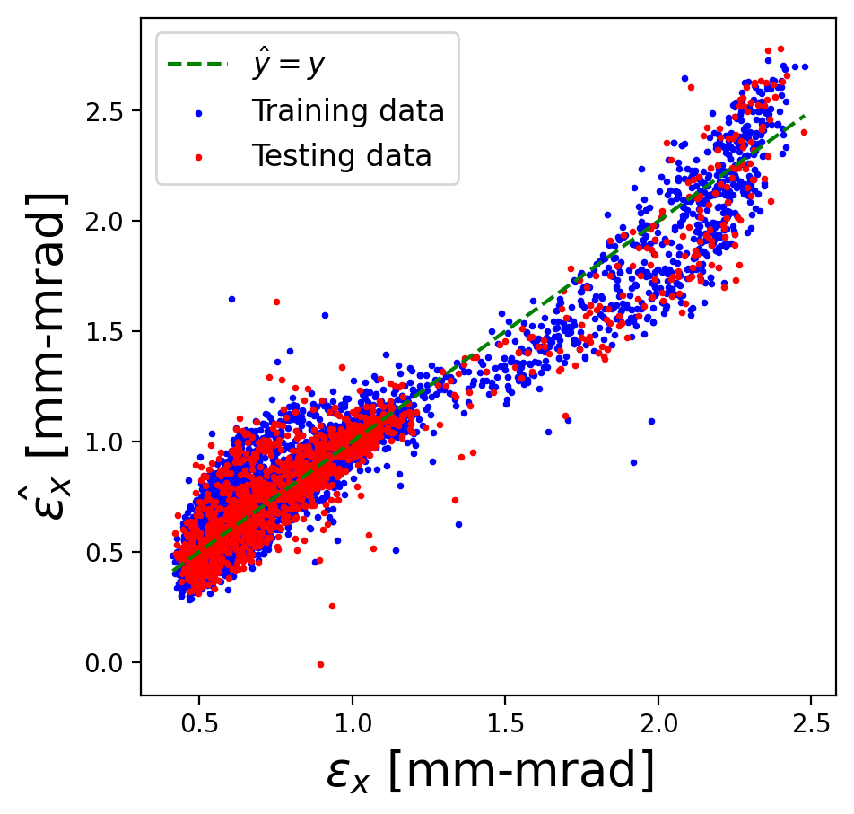
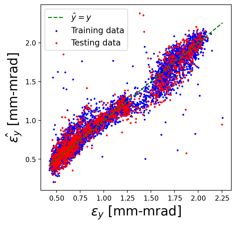
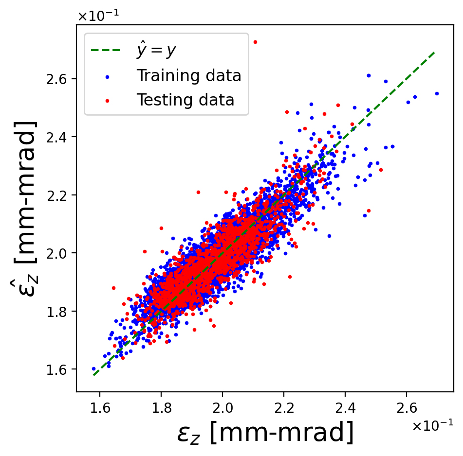
Figure 19: Surrogate model predicted value (indicated with a hat) versus OPAL simulation value of the projected emittances in all three planes, for training and testing points. The PCE model would perfectly replicate the high-fidelity simulations if all the points were lying on the 45^∘ dashed line.

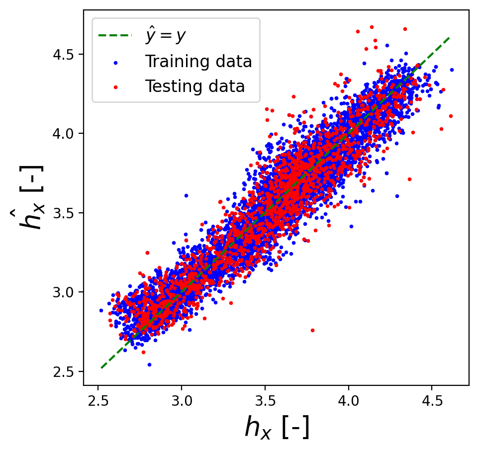
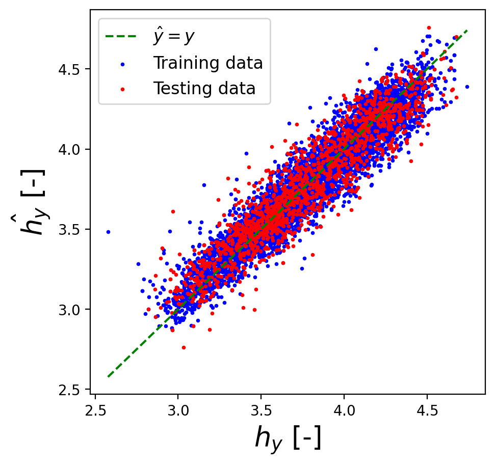
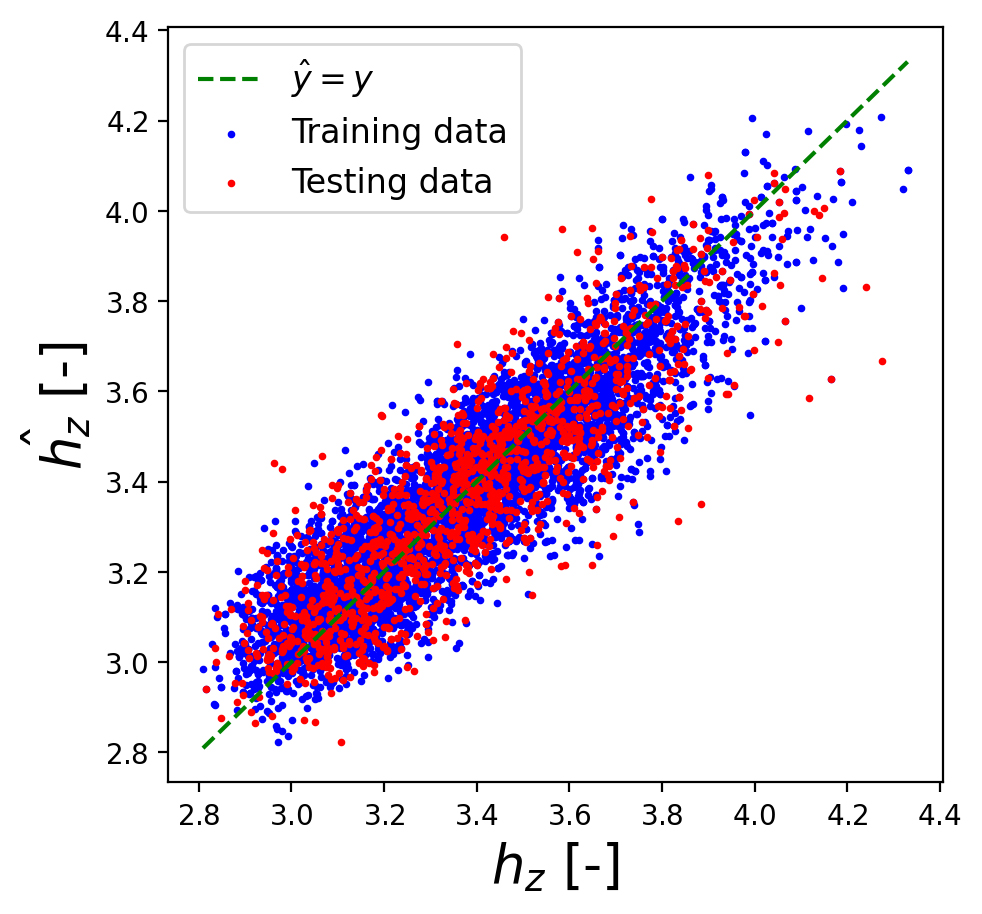
Figure 20: Surrogate model predicted value (indicated with a hat) versus OPAL simulation value of the halo parameters in all three planes, for training and validation points. The PCE model would perfectly replicate the high-fidelity simulations if all the points were lying on the 45^∘ dashed line.

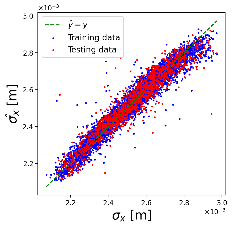
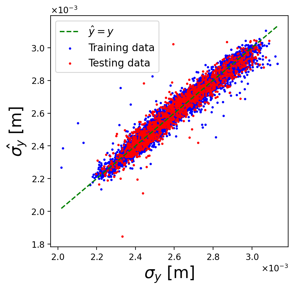
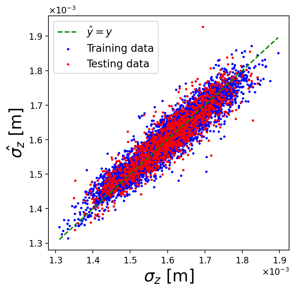
Figure 21: Surrogate model predicted value (indicated with a hat) versus OPAL simulation value of the RMS beam sizes in all three planes, for training and validation points. The PCE model would perfectly replicate the high-fidelity simulations if all the points were lying on the 45^∘ dashed line.

Table 6: Mean Absolute Error (MAE) of the surrogate models in percentage for the training and the testing sets.

	MAE train [%]	MAE test [%]
$\epsilon_{x}$ [mm-mrad]	9.397187	11.643873
$\epsilon_{y}$ [mm-mrad]	7.621135	9.097649
$\epsilon_{z}$ [mm-mrad]	2.065314	2.378235
$h_{x}$ [-]	2.776718	3.372337
$h_{y}$ [-]	2.477438	2.968650
$h_{z}$ [-]	2.635573	3.027616
$\sigma_{x}$ [m]	1.221384	1.521169
$\sigma_{y}$ [m]	1.250924	1.521905
$\sigma_{z}$ [m]	1.571111	1.760405

5.4 Discussion of Uncertainty Quantification

The IsoDAR cyclotron uncertainty quantification shows that the computational model and the physics model are consistent with each other, and gives credibility to the design. Furthermore, the advantage of surrogate modeling is that we obtain a black-box that reasonably predicts the output of a costly high-fidelity simulation given certain design variables at a fraction of the computational cost. These surrogate models are orders of magnitude faster [55] than the OPAL simulation. This fact can be exploited in order to perform fast multi-objective optimisation, for example using a genetic algorithm [60]. This could be used to finding other optimal working points of the IsoDAR cyclotron in future studies. A first trial at finding another optimal working point within the bounds presented in Table 5 makes the optimization algorithm fall back to the original design values of the cyclotron, ensuring that it is indeed an optimum, and again verifying the robustness of the design.

6 Conclusion and Outlook

In this paper, we presented a mature design, and simulations thereof, for the IsoDAR 60 MeV/amu compact isochronous cyclotron, which accelerates 5 mA of $\mathrm{H}_{2}^{+}$. The molecular hydrogen ions can then be charge-stripped with a carbon foil, yielding 10 mA of protons. The primary application of this machine is a definitive search for sterile neutrinos, however, the applications in other areas of science and industry are numerous: Material research, isotope production, energy research, and CP-violation searches in the neutrino sector (the latter two when the IsoDAR cyclotron is used as an injector to a larger cyclotron).

In order to verify our design, an exhaustive simulation study, using the well-established particle-in-cell code OPAL with 1e5 to 1e6 particles per bunch, was performed. Space-charge was taken into account, as well as all external fields and termination of particles inside the cyclotron. The extraction channels were modeled in CAD software and 3D fields were imported into OPAL. Through the combined forces of the cyclotron magnet, the accelerating RF cavities, and the particles’ self-fields, a vortex-effect takes place, which we exploited to stabilize the bunch size and phase space in the longitudinal-radial plane. This led to clean extraction, when using a set of two electrostatic channels, where power deposition at the highest particle energies was kept below 50 W (a quarter of the 200 W safety limit established at PSI). This is sufficient to guarantee low activation of the cyclotron and hence allows for frequent hands-on maintenance. To our knowledge, this is the first particle accelerator actively designed to exploit the vortex effect to transport and accelerate high intensity beams.

In the presented study, we started the design and simulation process with the bunch already injected into the cyclotron and coasting at 193 keV/amu. Our ongoing work on radiofrequency-direct injection (RFQ-DIP), and a preliminary design of the cyclotron spiral inflector and central region (which we briefly described in Section 2) give us confidence that the particle distributions can be matched at that point and that the total losses from ion source extraction to cyclotron extraction are below 50 %, requiring only 10 mA of DC $\mathrm{H}_{2}^{+}$ beam from the ion source. A full start-to-end simulation of ion source, low energy beam transport, RFQ-buncher and central region, including space-charge in all parts of the line, is currently ongoing and a publication is forthcoming.

We have also presented a full uncertainty quantification (UQ) using machine learning (surrogate modeling with polynomial chaos expansion) to determine how sensitive our optimized design is with respect to variations of the beam input parameters. From the results we can conclude that small variations of input beam parameters within the expected limits can be tolerated according to the UQ and thus our design is robust. Furthermore the computational model is shown to be consistent with the physics.

In addition, we propose a novel method to protect the extraction channel, in which $\mathrm{H}_{2}^{+}$ particles that would hit the septum are broken up into protons by means of a narrow stripper foil placed upstream of the septum. These protons will be bent inside of the septum, and follow a trajectory that takes them safely outside the cyclotron into either a beam dump, or a medical isotope target. Having this option is a direct consequence of the novel concept of using $\mathrm{H}_{2}^{+}$ for acceleration.

Other future work also includes multi-bunch simulations, wherein OPAL injects five bunches in sequence (one per full turn for five turns) to account for the space charge effect of neighboring bunches. This was done for an earlier iteration of our cyclotron design and the results were not dramatically changed. If anything, they were slightly improved when neighboring bunches “pushed” against each other through space charge.

References

References

- [1] Bungau A, Adelmann A, Alonso J R, Barletta W, Barlow R, Bartoszek L, Calabretta L, Calanna A, Campo D, Conrad J M, Djurcic Z, Kamyshkov Y, Shaevitz M H, Shimizu I, Smidt T, Spitz J, Wascko M, Winslow L A and Yang J J 2012 Phys. Rev. Lett. 109(14) 141802 URL http://link.aps.org/doi/10.1103/PhysRevLett.109.141802
- [2] Adelmann A, Alonso J R, Barletta W, Barlow R, Bartoszek L, Bungau A, Calabretta L, Calanna A, Campo D, Conrad J M, Djurcic Z, Kamyshkov Y, Owen H, Shaevitz M H, Shimizu I, Smidt T, Spitz J, Toups M, Wascko M, Winslow L A and Yang J J 2012 arxiv:1210.4454 [physics.acc-ph]
- [3] Abs M, Adelmann A, Alonso J, Axani S, Barletta W, Barlow R, Bartoszek L, Bungau A, Calabretta L et al. 2015 arXiv preprint arXiv:1511.05130
- [4] Schmor P 2010 Review of cyclotrons used in the production of radioisotopes for biomedical applications Proceedings of CYCLOTRONS pp 419–424
- [5] Alonso J R, Barlow R, Conrad J M and Waites L H 2019 Nature Reviews Physics 1 533–535 ISSN 2522-5820 URL https://www.nature.com/articles/s42254-019-0095-6
- [6] Waites L H, Alonso J R, Barlow R and Conrad J M 2020 EJNMMI Radiopharmacy and Chemistry 5 6 ISSN 2365-421X URL https://doi.org/10.1186/s41181-020-0090-3
- [7] Jepeal S J et al. 2020 Submitted to the Journal of Materials and Design
- [8] Jepeal S J et al. 2020 Submitted to the Nucl. Instr. and Meth. B
- [9] Zinkle S J and Snead L L 2018 Scripta Materialia 143 154–160 ISSN 1359-6462 URL https://doi.org/10.1016/j.scriptamat.2017.06.041
- [10] Vincent J, Blosser G, Horner G, Smirnov V, Stevens K, Usher N, Vorozhtsov S and Wu X 2016 Proceedings of Cyclotrons 2016, Zurich Switzerland
- [11] Moeslang A, Heinzel V, Matsui H and Sugimoto M 2006 Fusion Engineering and Design 81 863–871 ISSN 0920-3796 URL http://www.sciencedirect.com/science/article/pii/S0920379605005995
- [12] Ishi Y, Inoue M, Kuriyama Y, Mori Y, Uesugi T, Lagrange J, Planche T, Takashima M, Yamakawa E, Imazu H et al. 2010 Present status and future of FFAGs at KURRI and the first ADSR experiment Proceedings of IPAC10, Kyoto p 1323
- [13] Rubbia C, Roche C, Rubio J A, Carminati F, Kadi Y, Mandrillon P, Revol J P C, Buono S, Klapisch R, Fiétier N et al. 1995 Conceptual design of a fast neutron operated high power energy amplifier Tech. rep. CERN
- [14] Biarrotte J, Uriot D, Bouly F, Vandeplassche D and Carneiro J 2013 Design of the MYRRHA 17-600 MeV superconducting linac Proceedings of SRF13
- [15] Lisowski P 1997 The accelerator production of tritium Proceedings of PAC97 vol 97 p 3780
- [16] Alonso J, Avignone F, Barletta W, Barlow R, Baumgartner H, Bernstein A, Blucher E, Bugel L, Calabretta L, Camilleri L et al. 2010 arXiv preprint arXiv:1006.0260
- [17] Aberle C, Adelmann A, Alonso J, Barletta W, Barlow R, Bartoszek L, Bungau A, Calanna A, Campo D et al. 2013 arXiv preprint arXiv:1307.2949
- [18] Abs M, Adelmann A, Alonso J, Barletta W, Barlow R, Calabretta L, Calanna A, Campo D, Celona L, Conrad J et al. 2012 arXiv preprint arXiv:1207.4895
- [19] Calabretta L, Celona L, Gammino S, Rifuggiato D, Ciavola G, Maggiore M, Piazza L, Alonso J, Barletta W et al. 2011 arXiv preprint arXiv:1107.0652
- [20] Conrad J M, Collaboration D et al. 2012 Nuclear Physics B-Proceedings Supplements 229 386–390
- [21] 2013 Cyclone 70 (IBA – Ion Beam Applications S.A.) http://www.iba-cyclotron-solutions.com/products-cyclo/cyclone-70
- [22] 2019 BEST 70p Cyclotron (Best Cyclotron Systems, Inc.) http://www.bestcyclotron.com/product_70p.html
- [23] Grillenberger J, Humbel J M, Mezger A C, Seidel M and Tron W 2013 Status and Further Development of the PSI High Intensity Proton Facility Proceedings of Cyclotrons2013, Vancouver BC p 3
- [24] Winklehner D, Conrad J, Smolsky J and Waites L 2020 arXiv:2008.12292 [physics] ArXiv: 2008.12292 URL http://arxiv.org/abs/2008.12292
- [25] Bungau A, Alonso J, Bartoszek L, Conrad J, Shaevitz M and Spitz J 2019 Journal of Instrumentation 14 P03001–P03001 ISSN 1748-0221 (2019), Publisher: IOP Publishing URL https://doi.org/10.1088%2F1748-0221%2F14%2F03%2Fp03001
- [26] Inoue K 2004 International Journal of Modern Physics A 19
- [27] Diaz A, Argüelles C A, Collin G H, Conrad J M and Shaevitz M H 2020 Physics Reports 884 1–59 ISSN 0370-1573 URL http://www.sciencedirect.com/science/article/pii/S0370157320302921
- [28] Seidel M, Adam S R A, Adelmann A and Baumgarten C 2010 Production of a 1.3 MW Proton Beam at PSI Proceedings of IPAC’10, Kyoto, Japan p 5
- [29] Calanna A, Campo D, Yang J J, Calabretta L, Rifuggiato D, Maggiore M M, Piazza L A C and Adelmann A 2012 A Compact High Intensity Cyclotron Injector for DAEdALUS Experiment Proceedings, 3rd International Conference on Particle accelerators (IPAC 2012) vol C1205201 pp 424–426 URL http://accelconf.web.cern.ch/AccelConf/IPAC2012/papers/moppd027.pdf
- [30] Winklehner D, Hamm R, Alonso J, Conrad J M and Axani S 2015 Review of Scientific Instruments 87 02B929 ISSN 0034-6748 publisher: American Institute of Physics URL https://aip.scitation.org/doi/full/10.1063/1.4935753
- [31] Winklehner D, Bahng J, Calabretta L, Calanna A, Chakrabarti A, Conrad J, D’Agostino G, Dechoudhury S, Naik V, Waites L et al. 2018 Nuclear Instruments and Methods in Physics Research Section A: Accelerators, Spectrometers, Detectors and Associated Equipment 907 231–243
- [32] Campo D, Alonso J, Barletta W, Bartoszek L, Calanna A, Conrad J, Toups M and Shaevitz M 2013 High intensity compact cyclotron for IsoDAR experiment Proceedings of Cyclotrons2013, Vancouver, Canada URL http://epaper.kek.jp/CYCLOTRONS2013/papers/weppt030.pdf
- [33] 2021 CST Studio Suite 3D EM simulation and analysis software https://www.3ds.com/products-services/simulia/products/cst-studio-suite/
- [34] 2021 Opera | SIMULIA by Dassault Systems https://www.3ds.com/products-services/simulia/products/opera/
- [35] Joho W 1981 High Intensity Problems in Cyclotrons 9th International Conference on Cyclotrons and their Applications p 11
- [36] Axani S, Winklehner D, Alonso J and Conrad J M 2016 Review of Scientific Instruments 87 02B704
- [37] Conjat M and Mandrillon P 2018 Central Region studies for the IsoDAR test cyclotron Tech. rep. AIMA Developpement
- [38] Winklehner D, Adelmann A, Gsell A, Kaman T and Campo D 2017 Physical Review Accelerators and Beams 20 124201 URL https://link.aps.org/doi/10.1103/PhysRevAccelBeams.20.124201
- [39] Adelmann A, Calvo P, Frey M, Gsell A, Locans U, Metzger-Kraus C, Neveu N, Rogers C, Russell S, Sheehy S, Snuverink J and Winklehner D 2019 arXiv:1905.06654 [physics] ArXiv: 1905.06654 URL http://arxiv.org/abs/1905.06654
- [40] 2020 Comsol: Multiphysics software for optimizing designs https://www.comsol.com/
- [41] The HDF Group 2000-2010 Hierarchical Data Format version 5 http://www.hdfgroup.org/HDF5
- [42] 2021 Python Software Foundation. Python Language Reference, version 3.8. http://www.python.org
- [43] Yang J, Adelmann A, Humbel M, Seidel M, Zhang T et al. 2010 Physical Review Special Topics-Accelerators and Beams 13 064201
- [44] Kolano A, Adelmann A, Barlow R and Baumgarten C 2018 Nuclear Instruments and Methods in Physics Research Section A: Accelerators, Spectrometers, Detectors and Associated Equipment 885 54–59 ISSN 0168-9002 URL http://www.sciencedirect.com/science/article/pii/S0168900217314511
- [45] Kleeven W 2016 Some Examples of Recent Progress of Beam-Dynamics Studies for Cyclotrons 21st International Conference on Cyclotrons and their Applications p 7
- [46] Stetson J, Adam S, Humbel M, Joho W and Stammbach T 1992 The commissioning of PSI injector 2 for high intensity, high quality beams 13th International Conference on Cyclotrons and their Applications p 4
- [47] Koscielniak S R and Adam S R 1993 Simulation of space-charge dominated beam dynamics in an isochronous AVF cyclotron Proceedings of International Conference on Particle Accelerators pp 3639–3641 vol.5
- [48] Adam S 1985 Calculation of space charge effects in isochronous cyclotrons IEEE Transactions on Nuclear Science vol 32-5 pp 2507–2509 ISSN 1558-1578
- [49] Bertrand P and Ricaud C 2001 Specific cyclotron correlations under space charge effects in the case of spherical beam 16th International Conference on Cyclotrons and their Applications (AIP Conference Proceedings) pp 379–382 URL https://cds.cern.ch/record/536176
- [50] Baumgarten C 2011 Physical Review Special Topics-Accelerators and Beams 14 114201
- [51] Baumgarten C 2020 Proceedings of the 22nd International Conference on Cyclotrons and their Applications Cyclotrons2019 5 pages, 0.661 MB artwork Size: 5 pages, 0.661 MB ISBN: 9783954502059 Medium: PDF Publisher: JACoW Publishing, Geneva, Switzerland URL http://jacow.org/cyclotrons2019/doi/JACoW-Cyclotrons2019-WEB03.html
- [52] 2021 The OPAL Framework: Version 2.4 http://amas.web.psi.ch/opal/Documentation/2.4/index.html
- [53] 2021 Inventor | Mechanical Design & 3D CAD Software | Autodesk https://www.autodesk.com/products/inventor/overview
- [54] Yang J, Adelmann A, Barletta W, Calabretta L, Calanna A, Campo D and Conrad J 2013 Nuclear Instruments and Methods in Physics Research Section A: Accelerators, Spectrometers, Detectors and Associated Equipment 704 84 – 91 ISSN 0168-9002
- [55] Adelmann A 2019 SIAM/ASA Journal on Uncertainty Quantification 7 383–416
- [56] Sobol I 2001 Mathematics and Computers in Simulation 55 271 – 280 ISSN 0378-4754 the Second IMACS Seminar on Monte Carlo Methods
- [57] Frey M and Adelmann A 2021 Computer Physics Communications 258 107577 ISSN 0010-4655 URL http://www.sciencedirect.com/science/article/pii/S0010465520302770
- [58] Sudret B 2008 Reliability Engineering & System Safety 93 964 – 979 ISSN 0951-8320 bayesian Networks in Dependability URL http://www.sciencedirect.com/science/article/pii/S0951832007001329
- [59] Debusschere B, Sargsyan K, Safta C and Chowdhary K 2017 The uncertainty quantification toolkit (uqtk) Handbook of Uncertainty Quantification ed Ghanem R, Higdon D and Owhadi H (Springer) pp 1807–1827
- [60] Edelen A, Neveu N, Huber Y, Frey M and Adelmannn A 2020 Phys. Rev. AB 23 044601 URL https://link.aps.org/doi/10.1103/PhysRevAccelBeams.23.044601