Combinatorial generation via permutation languages.
III. Rectangulations
Abstract.
A generic rectangulation is a partition of a rectangle into finitely many interior-disjoint rectangles, such that no four rectangles meet in a point.In this work we present a versatile algorithmic framework for exhaustively generating a large variety of different classes of generic rectangulations.Our algorithms work under very mild assumptions, and apply to a large number of rectangulation classes known from the literature, such as generic rectangulations, diagonal rectangulations, 1-sided/area-universal, block-aligned rectangulations, and their guillotine variants, including aspect-ratio-universal rectangulations.They also apply to classes of rectangulations that are characterized by avoiding certain patterns, and in this work we initiate a systematic investigation of pattern avoidance in rectangulations.Our generation algorithms are efficient, in some cases even loopless or constant amortized time, i.e., each new rectangulation is generated in constant time in the worst case or on average, respectively.Moreover, the Gray codes we obtain are cyclic, and sometimes provably optimal, in the sense that they correspond to a Hamilton cycle on the skeleton of an underlying polytope.These results are obtained by encoding rectangulations as permutations, and by applying our recently developed permutation language framework.
Key words and phrases:
Exhaustive generation, Gray code, flip graph, polytope, generic rectangulation, diagonal rectangulation, cartogram, floorplan, permutation pattern1. Introduction
Partitioning a geometric shape into smaller shapes is a fundamental theme in discrete and combinatorial geometry.In this paper we consider rectangulations, i.e., partitions of a rectangle into finitely many interior-disjoint rectangles.Such partitions have an abundance of practical applications, which motivates their combinatorial and algorithmic study.For example, rectangulations are an appealing way to represent geographic information as a cartogram.This is a map where each country is represented as a rectangle, the adjacencies between rectangles correspond to those between countries, and the areas of the rectangles are determined by some geographic variable, such as population size [vKS07].If the rectangulation is area-universal [EMSV12] or aspect-ratio-universal [FNT21], respectively, then such an adjacency-preserving cartogram can be drawn for any assignment of area values or aspect ratios to the rectangles.Another important use of rectangulations is as floorplans in VLSI design and architectural design.These problems often involve additional constraints on top of adjacency, such as extra space for wires [Ott82] or proportion limits for the rooms [MSL76].An important notion in this context are slicing floorplans [Ott82], also known as guillotine floorplans, i.e., floorplans that can be subdivided into their constituent rectangles by a sequence of straight vertical or horizontal cuts.Rectangulations have rich combinatorial properties, and a task that has received a lot of attention is counting, i.e., determining the number of rectangulations of a particular type with rectangles, either exactly as a function of [YCCG03] or asymptotically as grows [SC03].This led to several beautiful bijections of rectangulations with pattern-avoiding permutations [ABP06a, Rea12, ABBM+13] or with twin binary trees [YCCG03].The focus of this paper is on another fundamental algorithmic task, which is more fine-grained than counting, namely exhaustive generation, meaning that every rectangulation from a given class must be produced exactly once.While such generation algorithms are known for many other discrete objects such as permutations, combinations, subsets, trees etc. and covered in standard textbooks such as Knuth’s [Knu11], much less is known about the generation of geometric objects such as rectangulations.The ultimate goal for a generation algorithm is to produce each new object in time , which requires that consecutively generated objects differ only by a ‘small local change’.Such a minimum change listing of combinatorial objects is often called a Gray code [Sav97].If the time bound for producing the next object holds in every step, then the algorithm is called loopless [Ehr73], and if it holds on average it is called constant amortized time (CAT) [Rus16].The Gray code problem entails the definition of a flip graph, which has as nodes all the combinatorial objects to be generated, and an edge between any two objects that differ in the specified small way.Clearly, computing a Gray code ordering of the objects is equivalent to traversing a Hamilton path or cycle in the corresponding flip graph.It turns out that some interesting flip graphs arising from rectangulations can be equipped with a natural lattice structure [Mee19], analogous to the Tamari lattice on triangulations, and realized as polytopes in high-dimensional space [LR12], analogous to the associahedron (see [PPR21] for generalizations).This ties in the Gray code problem with deep methods and results from lattice and polytope theory.
1.1. Our results
The main contribution of this paper is a versatile algorithmic framework for generating a large variety of different classes of generic rectangulations, i.e., rectangulations with the property that no four rectangles meet in a point.In particular, we obtain efficient generation algorithms for several interesting classes known from the literature, in some cases loopless or CAT algorithms; see Table 1.1.The initialization time and memory requirement for all these algorithms is linear in the number of rectangles.The classes of rectangulations shown in the table arise from generic rectangulations by imposing structural constraints, such as the guillotine property or forbidden configurations, or by equivalence relations, and they will be defined in Section 2.2.We implemented the algorithms generating the classes of rectangulations from the table in C++, and we made the code available for download and experimentation on the Combinatorial Object Server [cos].
| Class | Forbidden patterns | Counts/OEIS [oei20] | Refs. | Runtime | |
| generic |
: 2-clumped permutations |
A342141 |
[Rea12, Mee19] |
CAT
Thm. 12 |
|
|
diagonal
=mosaic floorpl. /R-equivalence |
: Baxter : twisted Baxter |
A001181 (Baxter numbers) |
[YCCG03, ABP06a, LR12, CSS18] |
LL
Thm. 15 |
|
|
1-sided
=area-universal |
|
[EMSV12, Lei21] |
Thm. 19 |
||
| block-aligned /S-equivalence |
n/a
|
A214358 |
[ABBM+13] |
LL
Thm. 37 |
|
| guillotine | generic |
|
Thm. 19 |
||
|
diagonal
=slicing fl.pl. /R-equiv. |
: separable |
A006318 (Schröder numbers) |
[YCCG03, ABP06a, AM10, ABBM+13] |
Thm. 19 |
|
|
1-sided
=aspect-ratio-universal |
|
A078482 |
[AM10, FNT21, Lei21] |
Thm. 19 |
|
|
|
A006012 |
[AM10] |
Thm. 19 |
||
|
block-aligned
/S-equiv. |
n/a
|
A078482 |
[ABBM+13] |
Thm. 38 |
|
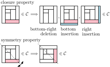
The classes of rectangulations that our algorithms can generate are not limited to the examples shown in Table 1.1, but can be described by the following closure property; see Figure 1.Given an infinite class of rectangulations , we require that if a rectangulation is contained in , then the rectangulation obtained from by deleting the bottom-right rectangle is also in , and the two rectangulations obtained from by inserting a new rectangle at the bottom or right, respectively, are also in (formal definitions of deletion and insertion are given in Section 2).If satisfies this property, then our algorithms allow generating the set of all rectangulations from with exactly rectangles, for every , by so-called jumps, a minimum change operation that generalizes simple flips, T-flips, and wall slides studied in [Rea12, CSS18] (the formal definition of jumps is in Section 3.1).Moreover, if the class is symmetric, i.e., if is in then the rectangulation obtained from by reflection at the diagonal from top-left to bottom-right is also in , then the jump Gray code for is cyclic, i.e., the last rectangulation differs from the first one only by a jump.In other words, we not only obtain a Hamilton path in the corresponding flip graph, but a Hamilton cycle.In fact, all the classes of rectangulations listed in Table 1.1 satisfy the aforementioned closure and symmetry properties, so in all those cases we obtain cyclic jump Gray codes.Generic rectangulations and diagonal rectangulations, shown in the first two rows of Table 1.1, have an underlying lattice and polytope structure [LR12, Mee19], and in those two cases our Gray codes form a Hamilton cycle on the skeleton of this polytope, i.e., jumps are provably optimal minimum change operations.The Gray codes for these two rectangulation classes with rectangles are shown in the appendix.
It turns out that many interesting classes of rectangulations can be characterized by pattern avoidance; see the second column in Table 1.1.Under very mild conditions on the patterns, these classes satisfy the aforementioned closure property, and can hence be generated by our framework.In this work we initiate a systematic investigation of pattern avoidance in rectangulations, and we obtain the first counting results for many known and new classes; see the third column in Table 1.1 and the more extensive tables in Section 10.Our generation framework for rectangulations consists of two main algorithms.The first is a simple greedy algorithm that generates a jump Gray code ordering for any set of rectangulations for which satisfies the aforementioned closure property; see Algorithm J□ and Theorem 5 in Section 3.The second is a memoryless version of the first algorithm, which computes the same ordering of rectangulations; see Algorithm M□ and Theorem 8 in Section 5.This algorithm can be fine-tuned to derive efficient algorithms for several known rectangulation classes such as the ones listed in Table 1.1, by providing corresponding jump oracles for the class .To prove Theorems 5 and 8, we encode rectangulations by permutations as described by Reading [Rea12], and we then apply our framework for exhaustively generating permutation languages presented in [HHMW20, HHMW21, HM21].The minimum change operations on permutations used in that framework translate to jumps on rectangulations.Generating different classes of rectangulations efficiently is thus another major new application of our permutation language framework, and in this paper we flesh out the details of this application.
1.2. Related work
There has been some prior work on generating a few special classes of rectangulations, all based on Avis and Fukuda’s reverse search method [AF96].Specifically, Nakano [Nak01] described a CAT generation algorithm for generic rectangulations, which does not produce a Gray code, however.This algorithm has been adapted by Takagi and Nakano [TN04] to generate generic rectangulations with bounds on the number of rectangles that do not touch the outer face.Yoshii, Chigira, Yamanaka and Nakano [YCYN06] gave a Gray code for generic rectangulations based on a generating tree that is different from ours, resulting in a loopless algorithm.Their Gray code changes at most 3 edges of the rectangulation in each step, whereas our algorithm changes only 1 edge in each step for generic and for diagonal rectangulations.Consequently, none of the listings produced by these earlier algorithms corresponds to a walk along the skeleton of the underlying polytope.There has been a lot of work on combinatorial properties of rectangulations.Yao, Chen, Cheng and Graham [YCCG03] showed that diagonal rectangulations are counted by the Baxter numbers and that guillotine diagonal rectangulations are counted by the Schröder numbers, using a bijection between diagonal rectangulations and twin binary trees.Ackerman, Barequet and Pinter [ABP06a] presented another bijection between diagonal rectangulations and Baxter permutations, which also yields a bijection between guillotine diagonal rectangulations and separable permutations.Leifheit [Lei21] showed that this bijection can be restricted to the 1-sided variants of these two rectangulation classes by adding two permutation patterns; see Table 1.1.Shen and Chu [SC03] provided asymptotic estimates for diagonal rectangulations and their guillotine variant.Moreover, He [He14] presented an optimal encoding of diagonal rectangulations with rectangles using only bits, which is optimal.The term ‘generic rectangulation’ was coined by Reading [Rea12], who established a bijection between generic rectangulations and 2-clumped permutations, proving that these permutations are representatives of equivalence classes of a lattice congruence of the weak order on the symmetric group.Earlier, generic rectangulations had been studied under the name ‘rectangular drawings’ by Amano, Nakano and Yamanaka [ANY07] and by Inoue, Takahashi and Fujimaki [FIT09, ITF09], who established recursion formulas and asymptotic bounds for their number.More general classes of rectangular partitions were analyzed by Conant and Michaels [CM14].Ackerman, Barequet and Pinter [ABP06b] considered the setting where we are given a set of points in general position in a rectangle, and the goal is to partition the rectangle into smaller rectangles by walls, such that each point from the set lies on a distinct wall.They showed that for every set of points that forms a separable permutation in the plane, the number of possible rectangulations is the st Baxter number, and for every point set the number of possible guillotine rectangulations is the th Schröder number.They also presented a counting and generation procedure based on simple flips and T-flips using reverse search, which was later improved by Yamanaka, Rahman and Nakano [YRN18].
1.3. Outline of this paper
In Section 2 we provide basic definitions and concepts that will be used throughout the paper.In Section 3 we present a greedy algorithm for generating a set of rectangulations by jumps, and we provide a sufficient condition for the algorithm to succeed.In Section 4 we show that the algorithm applies to a large number of rectangulation classes that are characterized by pattern avoidance.In Section 5 we demonstrate how to make our generation algorithm memoryless and efficient.The implementation details for our algorithms are provided in Sections 6 and 7.The proofs of Theorems 5 and 8 are presented in Section 8, by establishing a connection between rectangulations and permutations and by applying our permutation language framework.The results for one special class of rectangulations mentioned in Table 1.1 are deferred to Section 9.In Section 10 we report on our computer experiments about counting pattern-avoiding rectangulations.We conclude the paper with some interesting open questions in Section 11.Several visualizations of Gray codes produced by our algorithms are shown in the appendix.
2. Preliminaries
2.1. Generic rectangulations
A generic rectangulation, or rectangulation for short, is a partition of a rectangle into finitely many interior-disjoint axis-aligned rectangles, such that no four rectangles of the partition have a point in common; see Figure 2.In other words, every point where three rectangles meet, or where two rectangles meet the outer face forms a T-joint with the incident rectangle boundaries.Given rectangles and , we say that is left of , and is right of , if the right side of intersects the left side of (necessarily in a line segment, rather than a single point).Similarly, we say that is below , and is above , if the top side of intersects the bottom side of .We consider generic rectangulations up to equivalence that preserves the left/right and below/above relations between rectangles, and we use , , to denote the set of all rectangulations with rectangles.We write for the unique rectangulation in , i.e., the rectangulation consisting of a single rectangle.
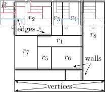
We refer to every rectangle corner in a rectangulation as a vertex, to every minimal line segment between two vertices as an edge, and to every maximal line segment between two vertices that are not corners of the rectangulation as a wall.The type of a vertex that is not a corner of the rectangulation describes the shape of the T-joint at this vertex, and it is one of , , , or .
2.2. Flip operations and classes of rectangulations
Our Gray codes use three types of local change operations on rectangulations; see Figure 3.
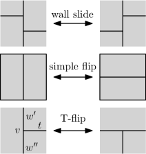
A wall slide swaps the order of two neighboring vertices of types and along a vertical wall, or of types and along a horizontal wall.A simple flip swaps the orientation of a wall that separates two rectangles.Given a vertex that belongs to three rectangles, we consider the wall that goes through and the wall that ends at , and we let and be the two halves of meeting in .If or is an edge, respectively, then a T-flip swaps the orientation of this edge so that it merges with .We now define various interesting subclasses of generic rectangulations that have been studied in the literature and that appear in Table 1.1.Examples illustrating these classes are in Figure 4.A diagonal rectangulation is one in which every rectangle intersects the main diagonal that goes from the top-left to the bottom-right corner of the rectangulation.We write for the set of all diagonal rectangulations with rectangles.Diagonal rectangulations are characterized by avoiding the wall patterns and [CSS18].Consider the equivalence relation on obtained from wall slides, sometimes referred to as R-equivalence [ABBM+13].The equivalence classes are referred to as mosaic floorplans, and every equivalence class contains exactly one diagonal rectangulation, obtained by repeatedly destroying occurrences of or by wall slides [CSS18].Consequently, in a diagonal rectangulation, along every vertical wall, all -vertices are below all -vertices, and along every horizontal wall, all -vertices are to the left of all -vertices.In a 1-sided rectangulation, every wall is the side of at least one rectangle, i.e., these rectangulations are characterized by avoiding the four patterns , , and .The notion of 1-sidedness was introduced by Eppstein, Mumford, Speckmann, and Verbeek [EMSV12] to characterize area-universal rectangulations, i.e., for any assignment of areas to the rectangles, the rectangulation can be drawn so that each rectangle has the prescribed area.Asinowski et al. [ABBM+13] also considered the equivalence relation on obtained from wall slides and simple flips, and they called it S-equivalence.By definition, S-equivalence is a coarser relation than R-equivalence, i.e., the equivalence classes are obtained by identifying mosaic floorplans that differ in simple flips.In Section 9 we introduce block-aligned rectangulations, which are a subset of diagonal rectangulations with the property that every equivalence class of S-equivalence contains exactly one block-aligned rectangulation.A rectangulation is guillotine, if each of its rectangles can be cut out from the entire rectangulation by a sequence of straight vertical or horizontal cuts.Guillotine rectangulations are characterized by avoiding the windmill patterns and , which is a folklore result.Various special classes of guillotine diagonal rectangulations, characterized by the avoidance of certain wall configurations, were introduced by Asinowski and Mansour [AM10] (see Section 4 for precise definitions of these configurations).Mosaic floorplans that are guillotine are also known as slicing floorplans.Felsner, Nathenson, and Tóth [FNT21] showed that 1-sided guillotine rectangulations are precisely the aspect-ratio-universal rectangulations, i.e., for any assignment of aspect ratios to the rectangles, the rectangulation can be drawn so that each rectangle has the prescribed aspect ratio.

2.3. Deletion of rectangles
We now describe two operations on a generic rectangulation , namely deleting a rectangle and inserting a rectangle.The resulting rectangulations will be denoted by and , notations that refer to the parent and children of , in a tree structure that will be discussed shortly.The deletion and insertion operations were introduced in [HHC+00] and heavily used e.g. in [ABP06a] and [Nak01].The idea of deletion is to contract the rectangle in the bottom-right corner of the rectangulation.Formally, given a rectangulation , , we consider the rectangle in the bottom-right corner, and we consider the top-left vertex of .If this vertex has type , then we collapse by sliding its top side, which forms a wall, downwards until it merges with the bottom side of ; see Figure 5 (a).Similarly, if this vertex has type , then we collapse by sliding its left side, which forms a wall, to the right until it merges with the right side of ; see Figure 5 (b).We denote the resulting rectangulation with rectangles by , and we say that is obtained from by deletion.
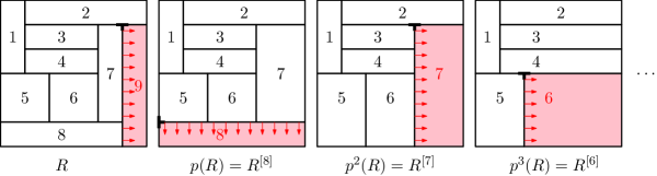
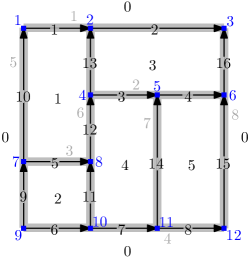
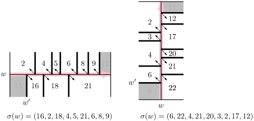
Moreover, we denote the rectangles of by in the order in which they are deleted when applying the deletion operation exhaustively; see Figure 6.Clearly, if is deleted and its top-left vertex has type , then the rightmost rectangle above is .Similarly, if the top-left vertex has type , then the lowest rectangle to the left of is .For any and we define , i.e., this is the sub-rectangulation of formed by the first rectangles; see Figure 6.
2.4. Insertion of rectangles
The idea of insertion is to add a new rectangle into the bottom-right corner of the rectangulation.Given a rectangulation , we first define a set of points in that can become the top-left corner of the newly added rectangle; see Figure 7.For any rectangle in , , that touches the bottom boundary of , we consider all edges forming the left side of , and from every such edge we select one interior point, and we refer to it as a vertical insertion point.

Similarly, for any rectangle in that touches the right boundary of , we consider the set of all edges forming the top side of , and from every such edge we select one interior point, and we refer to it as a horizontal insertion point.Combinatorially it does not make a difference which interior point of each edge is selected.We order the insertion points linearly, by sorting all vertical insertion points lexicographically by their -coordinates, followed by all horizontal insertion points sorted lexicographically by their -coordinates; see Figure 7.We write for the sequence of all insertion points ordered in this linear order.In particular, denotes the number of insertion points.
Lemma 1.
For any rectangulation we have .
Proof.
Each rectangle in has at most one vertical insertion point on its right side, and at most one horizontal insertion point on its bottom side.Moreover, no rectangle has both, the bottom-right rectangle has neither of the two, and exactly 2 insertion points lie on the boundary of .Combining these observations shows that .∎
Clearly, the upper bound in Lemma 1 is attained if every rectangle touches the bottom or right boundary of .Given and the sequence of insertion points , for each we define a rectangulation as follows:If is a vertical insertion point, then is obtained from by inserting a new rectangle in the bottom-right corner such that has above it exactly all rectangles which in lie to the right of and touch the bottom boundary of , and such that has to its left exactly all rectangles which in touch the vertical wall through below ; see Figure 8 (a).Similarly, if is a horizontal insertion point, then is obtained from by inserting a new rectangle in the bottom-right corner such that has to its left exactly all rectangles which in lie below and touch the right boundary of , and such that has above it exactly all rectangles which in touch the horizontal wall through to the right of ; see Figure 8 (b).We say that is obtained from by insertion.
By these definitions, the operations of deletion and insertion are inverse to each other, which we record in the following lemma.
Lemma 2.
For any rectangulation and any two distinct insertion points and from , the rectangulations and are distinct, and we have .Moreover, for any with there is an insertion point in such that .
The first and last insertion point play a special role in our arguments, which is why they are highlighted in Figure 8.We say that is bottom-based if has a rectangle whose bottom side is the entire bottom boundary of , and is right-based if has a rectangle whose right side is the entire right boundary of .Note that the rectangulation is both bottom-based and right-based, and if , then is bottom-based if and only if and right-based if and only if .
3. The basic algorithm
In this section we present the basic algorithm that we use to generate a set of rectangulations .
3.1. Jumps in rectangulations
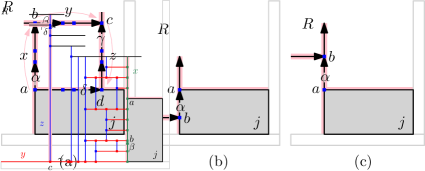
To state the algorithm, we first introduce a local change operation that generalizes the three kinds of flips introduced in Section 2.2 (recall Figure 3) and that will be applied when moving from one rectangulation in to the next in the algorithm.A jump changes the insertion point for exactly one rectangle of the rectangulation.Formally, for a rectangulation , we say that differs from by a right jump of rectangle by steps, denoted , where and , if one of the following conditions holds; see Figure 10:
-
•
, and we have , and for some ;
-
•
, and and are either both bottom-based or both right-based, and differs from in a right jump of rectangle by steps.
In words, the first condition asserts that the first rectangles in and form the same rectangulation , and and are obtained by insertion from using the th and th insertion point, respectively.The second condition asserts that and agree in the rectangle , which either forms the bottom boundary or the right boundary of those rectangulations, and differs from in a right jump with the same parameters.

A right jump as before is called minimal w.r.t. to a set of rectangulations , if in the first condition above there is no index with such that .A (minimal) left jump, denoted , is defined analogously by replacing by and by in the definitions above.Clearly, if differs from by a right jump of rectangle by steps, then differs from by a left jump of rectangle by steps, and vice versa, i.e., we have if and only if .We sometimes simply say that and differ in a jump, without specifying the direction left or right.We state the following simple observations for further reference; see Figure 9.
Lemma 3.
Consider two rectangulations that differ in a jump of rectangle , define , and let and be the insertion points in such that and .
-
(a)
If and are consecutive (w.r.t. ) on a common wall of , then and differ in a wall slide.
-
(b)
If lies on the last vertical wall and on the first horizontal wall of (w.r.t. ), then and differ in a simple flip.
-
(c)
If lies on a vertical wall and is the first insertion point on the next vertical wall of (w.r.t. ), or if lies on a horizontal wall and is the last insertion point on the previous horizontal wall, then and differ in a T-flip.
For any rectangulation , we say that two insertion points from belong to the same vertical or horizontal group, if they lie on the same vertical or horizontal wall in , respectively.In the sequence , insertion points belonging to the same group appear consecutively.

3.2. Generating rectangulations by minimal jumps
Consider the following algorithm that attempts to greedily generate a set of rectangulations using minimal jumps.Algorithm J□ (Greedy minimal jumps).This algorithm attempts to greedily generate a set of rectangulations using minimal jumps starting from an initial rectangulation .
-
J1.
[Initialize] Visit the initial rectangulation .
-
J2.
[Jump] Generate an unvisited rectangulation from by performing a minimal jump of the rectangle with largest possible index in the most recently visited rectangulation.If no such jump exists, or the jump direction is ambiguous, then terminate.Otherwise visit this rectangulation and repeat J2.
To illustrate how Algorithm J□ works, we consider the set of five rectangulations shown in Figure 11.If initialized with , then the algorithm performs a left jump of rectangle 4 by one step (a right jump of rectangle 4 is impossible) to reach , i.e., we have .In , there are two options, either a right jump of rectangle 4 by one step, leading back to , which has been visited before, or a left jump of rectangle 4 by two steps, leading to , so we visit .In , the jumps involving rectangle 4 lead to rectangulations that were visited before ( and ).Moreover, a jump of rectangle 3 does not lead to a rectangulation in .However, a right jump of rectangle 2 by one step leads to (a left jump of rectangle 2 is impossible), so we visit .Finally, in a right jump of rectangle 4 by two steps leads to (a left jump of rectangle 4 is impossible).In this example, Algorithm J□ successfully visits every rectangulation from exactly once.
On the other hand, suppose we instead initialize the algorithm with .The algorithm will then visit followed by , and then terminates without success, as from no jump leads to an unvisited rectangulation from .Lastly, suppose we initialize Algorithm J□ with .As before, in , there are two possibilities, either a right jump or a left jump of rectangle 4, both leading to an unvisited rectangulation from .Both are minimal jumps in opposite directions, and as the jump direction is ambiguous, the algorithm terminates immediately without success.
Remark 4.
We do not recommend using Algorithm J□ in the stated form to generate a set of rectangulations efficiently!This is because the algorithm requires to maintain the list of all previously visited rectangulations (possibly exponentially many), and to look up this list in each step to check whether a rectangulation obtained by a jump from the current one has been visited before.For us, Algorithm J□ is merely a tool to define a Gray code ordering of the rectangulations in the given set in way that is easy to remember (cf. [Wil13]).In fact, in Section 5 we will present a modified algorithm that dispenses with the costly lookup operations, and that computes the very same sequence of rectangulations.
3.3. A guarantee for success
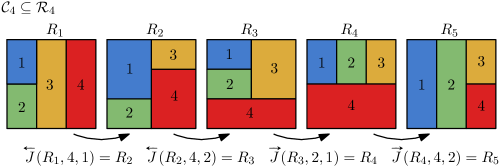
By definition, Algorithm J□ visits every rectangulation from a given set at most once, but it may terminate before having visited all.We now provide a sufficient condition guaranteeing that Algorithm J□ visits every rectangulation from exactly once.A set of generic rectangulations is called zigzag, if either and , or if and is zigzag and for every we have and .In words, the set must be closed under repeatedly deleting bottom-right rectangles and replacing them by rectangles inserted either below or to the right of the remaining ones; recall Figure 1.The name ‘zigzag’ does not refer to the shape of a rectangulation, but to the order in which they are visited by Algorithm J□, which will become clear momentarily.We also say that is symmetric, if reflection at the main diagonal is an involution of , i.e., if , then the rectangulation obtained from by reflection at the main diagonal is also in .We write for the rectangulation that consists of vertically stacked rectangles.
Theorem 5.
Given any zigzag set of rectangulations and initial rectangulation , Algorithm J□ visits every rectangulation from exactly once.Moreover, if is symmetric, then the ordering of rectangulations generated by Algorithm J□ is cyclic, i.e., the first and last rectangulation differ in a minimal jump.
The proof of Theorem 5 is provided in Section 8.Note that the rectangulation is contained in every zigzag set by definition, so this is a valid initialization for Algorithm J□.We write for the sequence of rectangulations generated by Algorithm J□ for a zigzag set when initialized with .It is easy to see that the number of distinct zigzag sets of generic rectangulations is at least (the latter estimate uses the best known lower bound on from [ANY07]), i.e., at least double-exponential in .In other words, Algorithm J□ exhaustively generates a given set of generic rectangulations in a vast number of cases.Moreover, many natural classes of rectangulations are in fact zigzag.In particular, all the different classes introduced in Section 2.2 and shown in Table 1.1 satisfy the aforementioned closure property.Moreover, all of these classes are symmetric, so for each of them we obtain cyclic jump orderings.Several such Gray codes are visualized in the appendix.
3.4. Tree of rectangulations
The notion of zigzag sets and the operation of Algorithm J□ can be interpreted combinatorially in the so-called tree of rectangulations, which is an infinite rooted tree, defined recursively as follows; see Figure 12:The root of the tree is a single rectangle .For any node , , of the tree we consider all insertion points of the rectangulation , and the set of children of in the tree is .Conversely, the parent of each , , is .In words, insertion leads to the children of a node, and deletion leads to the parent of a node.By Lemma 2, each generic rectangulation appears exactly once in the tree, and the set of nodes at distance from the root of the tree is precisely the set of generic rectangulations with rectangles.We emphasize that this tree is unordered, i.e., there is no specified ordering among the children of a node.By Lemma 1, a node in the tree has at most children, i.e., we have .As we see from Figure 12, this inequality is tight up to , but starting from , there are nodes with strictly less than children, i.e., we have .In fact, it was shown in [ANY07] that .A subset of nodes in depth of this tree is zigzag, if and only if it arises from the full tree of rectangulations by pruning some subtrees whose roots are neither bottom-based nor right-based rectangulations.In Figure 12, all bottom-based or right-based rectangulations are highlighted by gray boxes, and can therefore not be pruned, while all other nodes can possibly be pruned.If no nodes are pruned, then we have , and if all possible nodes are pruned, then is the set of rectangulations obtained by repeatedly stacking a new rectangle either below or to the right of the previous ones, i.e., for and .Moreover, we have for any zigzag set .
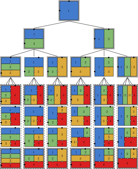
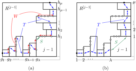
The operation of Algorithm J□ for a zigzag set as input can be interpreted as follows:Given the pruned tree corresponding to , we consider the set of nodes on all previous levels of the tree, i.e., the sets for , which are all zigzag sets by definition.Moreover, we consider the orderings , , defined by Algorithm J□ for each of these sets.These sequences turn the unordered tree corresponding to into an ordered tree, where the children of each node from left to right appear alternatingly in increasing order or in decreasing order .Consequently, in the sequence , , which forms the left-to-right sequence of all nodes in depth of this ordered tree, the rectangle alternatingly jumps left and right between the first and last insertion point, which motivates the name ‘zigzag’ set; see also the animations provided in [cos].It is important to realize that these orderings are not consistent with respect to taking subsets, i.e., if we have two zigzag sets , then the entries of the sequence do not necessarily appear in the same relative order in the sequence .
4. Pattern-avoiding rectangulations
In this section we show that Algorithm J□ applies to a large number of rectangulation classes that are defined by pattern avoidance, under some very mild conditions on the patterns; recall Table 1.1.A rectangulation pattern is a configuration of walls with prescribed directions and incidences.For example, the windmill patterns and describe four walls such that when considering the walls in clockwise or counterclockwise order, respectively, the end vertex of one wall lies in the interior of the next wall.We can also think of a pattern as the rectangulation formed by the given walls and incidences.For example, we can think of the windmill patterns as rectangulations with 5 rectangles.We say that a rectangulation contains the pattern , if contains a subset of walls with the directions and incidences specified by .Otherwise we say that avoids .For any set of rectangulation patterns and for any set of rectangulations , we write for the rectangulations from that avoid each pattern from .For example, diagonal rectangulations are given by .Examples of rectangulations containing and avoiding various patterns are shown in Figure 4.We say that a rectangulation pattern is tame, if for any rectangulation that avoids , we also have that and avoid .In words, inserting a new rectangle below or to the right of must not create the forbidden pattern .The next lemma follows directly from these definitions.
Lemma 6.
If a rectangulation pattern is neither bottom-based nor right-based, then it is tame.In particular, each of the patterns is tame.
The following powerful theorem allows to obtain many new zigzag sets of rectangulations from a given zigzag set by forbidding one or more tame patterns.All of these zigzag sets can then be generated by our Algorithm J□.
Theorem 7.
Let be a zigzag set of rectangulations, and let be a set of tame rectangulation patterns.Then is a zigzag set of rectangulations.Moreover, if is symmetric, then is symmetric.
Recall that is symmetric if for each pattern , we have that the pattern obtained from by reflection at the main diagonal is also in .The significance of the second part of the theorem is that if is symmetric, then the ordering of rectangulations of generated by Algorithm J□ is cyclic by Theorem 5.
Proof.
As is a zigzag set of rectangulations, we know that for are also zigzag sets.We argue by induction that is also a zigzag set for all .For the induction basis note that the rectangulation that consists of a single rectangle has no walls, so it avoids any pattern, showing that .For the induction step we assume that , , is a zigzag set, and we prove it for .Note that , and so we only need to check that and are in for all , which is guaranteed by the assumption that each pattern is tame.This proves the first part of the theorem.It remains to prove the second part.If , then avoids every pattern from .Let be the rectangulation obtained from by reflection at the main diagonal. must also avoid every pattern from , because if it contained a pattern from , then would contain the corresponding reflected pattern , which is in because of the assumption that is symmetric.It follows that , completing the proof.∎
5. Efficient computation
Recall from Remark 4 that Algorithm J□ in its stated form is unsuitable for efficient implementation.We now discuss how to make the algorithm efficient, so as to achieve the time bounds claimed in Table 1.1 for several interesting classes of rectangulations.
5.1. Memoryless algorithm
Consider Algorithm M□ below, which takes as input a zigzag set of rectangulations and generates them exhaustively by minimal jumps in the same order as Algorithm J□, i.e., in the order .After initialization in line M1, the algorithm loops over lines M2–M5, visiting the current rectangulation at the beginning of each iteration (line M2), until it terminates (line M3).The key idea of the algorithm is to track explicitly which rectangle jumps in each step, and the direction of the jump.With this information, the jump is determined by the condition that it must be minimal w.r.t. , i.e., starting from the current insertion point of the given rectangle, we choose the first insertion point (w.r.t. their linear ordering) for that rectangle in the given direction that creates the next rectangulation from .Algorithm M□ (Memoryless minimal jumps).This algorithm generates all rectangulations of a zigzag set by minimal jumps in the same order as Algorithm J□.It maintains the current rectangulation in the variable , and auxiliary arrays and .
-
M1.
[Initialize] Set , and , for .
-
M2.
[Visit] Visit the current rectangulation .
-
M3.
[Select rectangle] Set , and terminate if .
-
M4.
[Jump rectangle] In the current rectangulation , perform a jump of rectangle that is minimal w.r.t. , where the jump direction is left if and right if .
-
M5.
[Update and ] Set .If and is bottom-based set , or if and is right-based set , and in both cases set and . Go back to M2.
| jump | jump | |||||||||
|---|---|---|---|---|---|---|---|---|---|---|
| 1 | 1234 | 12 | 114 | |||||||
| 2 | 4 | 13 | 4 | |||||||
| 3 | 4 | 14 | 4 | |||||||
| 4 | 33 | 15 | 33 | |||||||
| 5 | 4 | 16 | 4 | |||||||
| 6 | 4 | 17 | 4 | |||||||
| 7 | 4 | 18 | 4 | |||||||
| 8 | 33 | 19 | 33 | |||||||
| 9 | 224 | 20 | 214 | |||||||
| 10 | 4 | 21 | 4 | |||||||
| 11 | 32 | 22 | 31 |
Specifically, the jump directions are maintained by an array , where means that rectangle performs a left jump in the next step, and means that rectangle performs a right jump in the next step (line M4).All sub-rectangulations of the initial rectangulation are right-based, so the initial jump directions are for (line M1).Whenever rectangle jumps left and reaches the first insertion point, which means that is bottom-based, or if it jumps right and reaches the last insertion point, which means that is right-based, then the jump direction is reversed (line M5).The array is used to determine which rectangle jumps in each step.Specifically, the last entry determines the rectangle that jumps in the current iteration (line M3).This array simulates a stack in a loopless fashion, following an idea first used by Bitner, Ehrlich, and Reingold [BER76].The stack is initialized by (line M1), with being the value on the top of the stack.The stack is popped (by the instruction in line M5) when rectangle reaches its first or last insertion point in this step, meaning that this rectangle is not eligible to jump in the next step, but becomes eligible again after the next step, which is achieved by pushing the value on the stack again (by the instructions and in line M5).Table 2 shows the execution of Algorithm M□ with input being the set of all diagonal rectangulations with 4 rectangles.
Theorem 8.
For any zigzag set of rectangulations , Algorithm M□ visits every rectangulation from exactly once, in the order defined by Algorithm J□.
The proof of Theorem 8 is provided in Section 8.To make meaningful statements about the running time of Algorithm M□, we need to specify the data structures used to represent the current rectangulation , and the operations on this data structure to perform jumps in line M4 and to check the bottom-based and right-based property in line M5.Most importantly, we will develop oracles which efficiently compute the next minimal jump w.r.t. for some interesting zigzag sets .One should think of here as a class of rectangulations specified by some properties or forbidden patterns, such as ‘diagonal guillotine rectangulations’, and not as a large precomputed set of rectangulations.All of these details are described in the following sections, and they are part of our C++ implementation provided in [cos].
6. Implementation details
In the following we describe the data structures we use to represent and manipulate generic rectangulations, and the efficient implementation of jump operations using those data structures.
6.1. Data structures
We represent a generic rectangulation with rectangles as follows; see Figure 13:Rectangles are stored in the variables , indexed by the reverse deletion order described in Section 2.3 (recall Figure 6).Vertices and edges are stored in variables and , respectively (indexed in no particular order).
|
|
|
|
Each vertex points to the edges incident to it in the four directions by , , , and .Some of these can be 0, indicating that no edge is incident.This information determines the type , which is one of , , , , or 0 at the corner vertices of the rectangulation.We give all edges a default orientation from left to right, or from bottom to top.The dir entry of each edge specifies its direction, which is either for a horizontal edge or for a vertical edge.Each edge points to its two end vertices, specifically to its tail by and to its head by (with respect to the default orientation).It also points to the previous and next edge, in the direction of its orientation, by and , respectively, which can be 0 if no such edge exists.The rectangle to the left and right side of an edge , in the direction of its orientation, are stored in and , which can be 0 at the boundary of the rectangulation.Each rectangle points to its four corner vertices by , , , and in the corresponding directions.For some rectangulation classes it is useful to store information about walls, i.e., maximal sequences of edges between two vertices that are not corners of the rectangulation.These are stored in , where for simplicity we also keep track of the four maximal line segments between corners of the rectangulation (which are not walls in our definition).We also think of walls having a default orientation from left to right, or from bottom to top, and each wall points to its first and last vertex by and , respectively, in the direction of its orientation.Moreover, each edge has an entry pointing to the wall that contains it.
Remark 9.
The aforementioned data structures are natural in the sense that they also capture the dual graph of the rectangulation, i.e., the graph obtained by replacing every rectangle by a vertex, and by joining any two vertices that correspond to rectangles sharing a common edge.This allows constructing the so-called transversal structure [Fus09] (also known as regular edge labeling [KH97]), which is useful for computing a layout of the rectangulation; see Felsner’s survey [Fel13].Our data structures also allow to easily extract the twin binary tree representation of diagonal rectangulations described in [YCCG03].
We now use these data structures for implementing jumps efficiently.Recall the conditions stated in Lemma 3 when a jump is one of the three flip operations shown in Figure 3.We refer to a jump as in (a), (b) or (c) in the lemma as a W-jump, S-jump, or T-jump, respectively.By these definitions, a W-jump is a special wall slide, an S-jump is a special simple flip, and a T-jump is a special T-flip.We refer to W-, S- and T-jump as local jumps collectively.Moreover, a W-jump or T-jump between two horizontal insertion points, or between two vertical insertion points, is referred to as a horizontal or vertical W- or T-jump, respectively.Consider two rectangulations and that differ in a jump of rectangle .If the jump is an S-jump or a horizontal T-jump, we let denote the number of horizontal insertion points of that lie in the interior of the top side of rectangle in or ; see Figure 14.Similarly, if the jump is an S-jump or a vertical T-jump, we let denote the number of vertical insertion points of that lie in the interior of the left side of rectangle in or .
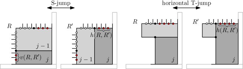
Lemma 10.
Local jumps can be implemented with the following time guarantees:
-
(a)
A W-jump takes time .
-
(b)
An S-jump between rectangulations and takes time .
-
(c)
A horizontal T-jump between rectangulations and takes time and a vertical T-jump takes time .
Clearly, every jump can be performed as a sequence of local jumps, and then the time bounds given by Lemma 10 can be added up.
Proof.
The time bounds follow from the number of incidences that change during local jumps.The crucial point is that during a jump of rectangle between and , all rectangles for are right-based or bottom-based in and , entailing that only constantly many incidences with such rectangles have to be modified.∎
6.2. Auxiliary functions
In Section 6.3 we provide implementations of local jumps with the runtime guarantees stated in Lemma 10.Before doing so, we introduce some auxiliary functions to add and remove edges from a rectangulation.These auxiliary functions only update the incidences between edges, vertices and walls, but not the incidences between rectangles and any other objects and the type of vertices (this will be done separately later).The following function removes the edge together with its head vertex.Function (Remove and its head).
-
1.
[Prepare] Set , , .
-
2.
[Update edges/vertices]If , set .If , set and .If , set .Otherwise we have and set .
-
3.
[Update wall] Set .If , set .
After defining some auxiliary variables in the first step, the function updates the incidences between edges and vertices in the second step, and the incidences between walls and edges in the third step.We also define an analogous function that removes and its tail instead of its head.For details, see our C++ implementation [cos].The following two functions and insert the edge with head or tail , respectively, before or after the edge or .Function (Insertion of with head before ).
-
1.
[Prepare] Set and .
-
2.
[Update edges/vertices] Set , , , , , , and if set .If , set , , and .Otherwise we have and set , , and .
-
3.
[Update wall] Set .
Function (Insertion of with tail after ).
-
1.
[Prepare] Set and .
-
2.
[Update edges/vertices] Set , , , , , , and if set .If , set , , and .Otherwise we have and set , , and .
-
3.
[Update wall] Set .
6.3. Local jumps
Armed with these auxiliary functions, we now tackle the implementation of local jumps with the time guarantees stated in Lemma 10.Each of the functions , and below takes as input the current rectangulation in which the jump is performed, the index of the rectangle to be jumped, the direction of the jump, and the index of the edge which contains the insertion point of that will become the top-left vertex of after the jump.In the pseudocode of these algorithms, all references to rectangles , edges , vertices or walls are with respect to the current rectangulation .We first present the implementation of W-jumps.For simplicity, we only show the implementation of left horizontal W-jumps in the function below; see Figure 15 (a).The implementation of right horizontal W-jumps, and of left and right vertical W-jumps in a function is very similar; we omit the details here.Function (left horizontal W-jump).
-
1.
[Prepare] Set , and .
-
2.
[Flip and update rectangles] Call and .Then set and .
The running time of is clearly , as claimed in part (a) of Lemma 10.We proceed with the implementation of S-jumps.For simplicity, we only provide the implementation of left S-jumps in the function below; see Figure 15 (b).The implementation of right S-jumps is very similar.
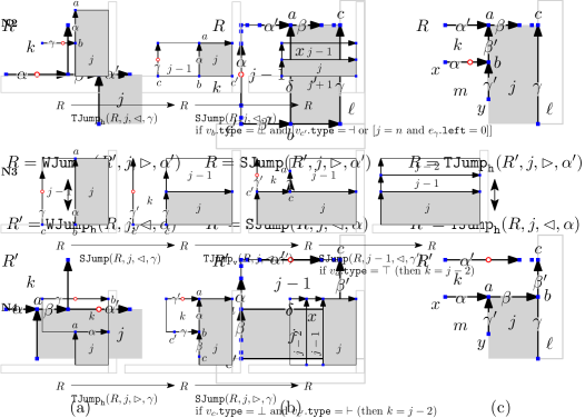
Function (left S-jump).
-
1.
[Prepare] Set , , , , , , , , , , and .
-
2.
[Flip] Call , , and .Then set , , , , , , , , , and .
-
3.
[Update rectangles]Set , , , and .Set , and while repeat and .Set , and while repeat and .Also set , , and .
Let be the rectangulation obtained from by one call of .The running time of this call is , as claimed in part (b) of Lemma 10.This time is incurred by the while-loops in step 3.Specifically, the first while-loop is iterated exactly times, and the second while-loop is iterated exactly times.We complete this section by presenting the implementation of T-jumps; see Figure 15 (c).For simplicity, we only provide the implementation of left horizontal T-jumps in the function below.The implementation of right horizontal T-jumps, and of left and right vertical T-jumps in a function is very similar.Function (left horizontal T-jump).
-
1.
[Prepare] Set , , , , , , , , , , , and .
-
2.
[Flip] Call , , and .Then set , , , , and .
-
3.
[Update rectangles]Set , and .Set , and while repeat and .Also set and .
Let be the rectangulation obtained from by one call of .The running time of this call is , as claimed in part (c) of Lemma 10.This time is incurred by the while-loop in step 3, which is iterated exactly times.
7. Minimal jump oracles
A minimal jump oracle is a function that is called in line M4 of Algorithm M□ to compute a jump in the current rectangulation that is minimal respect to the given zigzag set of rectangulations .In this section we specify such oracles for the zigzag sets mentioned in Table 1.1, which allows us to establish the runtime bounds for Algorithm M□ stated in the last column of the table (except for block-aligned rectangulations, which are handled in Section 9).A minimal jump oracle has the form , and this function call performs in the current rectangulation a jump of rectangle in direction that is minimal w.r.t. , and the function will modify accordingly.Depending on , our minimal jump oracles perform a suitable W-, S-, or T-jump, or a combination thereof, as implemented in the previous section.
7.1. Generic rectangulations
We first consider the case of generic rectangulations.Given the current rectangulation , upon a jump of rectangle in direction , every insertion from is used, so we simply need to detect the next one.By Lemma 3, a W-jump occurs between any two consecutive (w.r.t. ) insertion points belonging to the same horizontal or vertical group, an S-jump occurs between the last vertical insertion point and the first horizontal insertion point, and a T-jump occurs between the last insertion point of a group and the first insertion point of the next group, if both groups are vertical or horizontal.Specifically, suppose there are vertical groups and horizontal groups with cardinalities , , and , , respectively in (note that ).Then the jump sequence consisting of letters that specifies the types of jumps performed with rectangle from the first to the last insertion point is
| (1) |
see Figure 16 (a).Of course, during Algorithm M□, these jump operations are not consecutive, but they are interleaved with the jump sequences of other rectangles , .The details are spelled out in the function . (Minimal jump oracle for generic rectangulations).
-
N1.
[Prepare] Set .If and , set , , and and goto N2.If and , set , and goto N3.If and , set , , and and goto N4.If and , set , and goto N5.
-
N2.
[Horizontal left jump] If , set and call .Else if , set and call .Otherwise we have , set and call . Return.
-
N3.
[Horizontal right jump] If , set and call .Otherwise we have , set , and and call . Return.
-
N4.
[Vertical right jump] If , set and call .Else if , set and call .Otherwise we have , set and call . Return.
-
N5.
[Vertical left jump] If , set and call .Otherwise we have , set , and and call . Return.
The four distinct cases treated in lines N2–N4 come from the directions and whether the jump is horizontal or vertical.The latter condition is determined in line N1 by querying the type of the top-left vertex of , which is either or .Note that the code in lines N2 and N4 is symmetric by reflecting all directions at the main diagonal.The same holds for the code in lines N3 and N5.
Lemma 11.
Consider a rectangulation with insertion points.Then calling exactly times with initial rectangulation , yields for , and the total time for these calls is .An analogous statement holds for .
Proof.
If the sequence of insertion points has vertical groups and horizontal groups of cardinalities , , and , , respectively, then the sequence of jumps performed by the calls to has the form (1).We clearly have .We use Lemma 10 to bound the overall time to perform those operations; see Figure 16 (a).The number of W-jumps in (1) is .The sum of the terms and over any two consecutive rectangulations in this sequence that differ in a T-jump is and , respectively.The sum for the two consecutive rectangulations in this sequence that differ in an S-jump is .Clearly, we have .Consequently, the overall time for those operations is , as claimed.∎
Theorem 12.
Algorithm M□ with the minimal jump oracle takes time on average to visit each generic rectangulation.
Proof.
For some fixed , we consider all jumps of rectangle .Whenever rectangle jumps in a rectangulation , then is either bottom-based or right-based for all .Moreover, none of the rectangles jumps unless is bottom-based or right-based.Consequently, we can partition the jumps of in the entire jump sequence into subsequences, such that in each subsequence, for each rectangulation of the subsequence, is the same subrectangulation and in the rectangle jumps to the next insertion point of .By Lemma 11, the total time for visiting the many rectangulations of this subsequence is , which is on average.∎
Remark 13.
By slightly modifying our data structures, we could even obtain a loopless algorithm for generic rectangulations.The idea is to introduce an additional data structure called sides.Each rectangle is subdivided into four sides, and in the incidence relations, sides sit between edges and rectangles, i.e., edges do not point to the two touching rectangles directly, but to the relevant sides of those rectangles, and each side points to the rectangle it belongs to.During S-jumps and T-jumps, a rectangle can be broken up into its four sides and the sides of two rectangles can be interchanged in constant time, avoiding the while-loops in the functions Sjump and Tjump that need to update possibly linearly many incidences between edges and rectangles.To keep the presentation simple, we do not show these modifications.Also, the resulting improvement is not substantial, and sides are a somewhat artificial concept.
7.2. Diagonal rectangulations
Recall that in a diagonal rectangulation , every rectangle intersects the main diagonal, or equivalently, avoids the patterns and .Consequently, during a jump of rectangle in the current rectangulation , we need to consider precisely the insertion points from that are the first insertion point of a vertical group, or the last insertion point of a horizontal group, as any other insertion point from each group would create one of the forbidden pattern; see Figure 16 (b).Consequently, if the sequence has vertical groups and horizontal groups, then the jump sequence that specifies the types of jumps with rectangle from the first to the last insertion point is
In particular, we do not perform any wall slides.An implementation of this is provided in the function . (Minimal jump oracle for diagonal rectangulations).
-
N1.
[Prepare] Set .If and , set and and goto N2.If and , set and goto N3.If and , set and and goto N4.If and , set and goto N5.
-
N2.
[Horizontal left jump] If , set and call .Otherwise we have , set and and call .Return.
-
N3.
[Horizontal right jump] Set , and and call . Return.
-
N4.
[Vertical right jump] If , set and call .Otherwise we have , set and and call .Return.
-
N5.
[Vertical left jump] Set , and and call . Return.
Similarly to before, the code in lines N2 and N4, and in lines N3 and N5 is symmetric by reflecting all directions at the main diagonal.For diagonal rectangulations the runtime analysis is straightforward and gives a loopless algorithm.
Lemma 14.
Each call takes time .
Proof.
Let be the rectangulation after the call , which differs from in an S-jump or T-jump.As we only consider the first insertion point of each vertical group and the last insertion point of each horizontal group of , we have and .The claim now follows from Lemma 10 (b)+(c).∎
Lemma 14 immediately yields the following result.
Theorem 15.
Algorithm M□ with the minimal jump oracle takes time to visit each diagonal rectangulation.
Remark 16.
Jumps as performed by the oracles and and shown in Figure 16 correspond to cover relations in the lattice of generic rectangulations and the lattice of diagonal rectangulations described by Meehan [Mee19] and Law and Reading [LR12], respectively, which both arise as lattice quotients of the weak order on the symmetric group.Consequently, our cyclic Gray codes correspond to Hamilton cycles in the cover graphs of those lattices.In [HM21] we showed that our permutation language framework can be used to generate a Hamilton path on every lattice quotient of the weak order, which also yields a Hamilton path on the skeleton of the corresponding polytope [PS19] (see also [PPR21]).
7.3. Pattern-avoiding rectangulations
For any zigzag set of rectangulations , and any set of tame patterns , Theorem 7 guarantees that the set of rectangulations that avoid all patterns from is also a zigzag set.We now describe how we can obtain a minimal jump oracle for from a minimal jump oracle for .The idea is simply to perform a minimal jump of w.r.t. , and to test after each jump whether the resulting rectangulation contains any pattern from , repeating this process until we arrive at a rectangulation that avoids all patterns from .This is guaranteed to terminate after at most iterations, as the first and last insertion point of will produce rectangulations that avoid all patterns from , due to the zigzag property. (Minimal jump oracle for pattern-avoiding permutations).
-
N1.
[Fast forward] While contains a pattern from repeat .
We immediately obtain the following generic runtime bounds.
Theorem 17.
Let be a finite set of tame rectangulation patterns.If the zigzag set has a minimal jump oracle that runs in time , and containment of any pattern from in can be tested in time , then is a minimal jump oracle for that runs in time .
In some cases the runtime bound for at most consecutive calls of or several consecutive pattern containment tests can be improved upon the trivial bounds and , respectively (see the proof of Theorem 19 below).Moreover, for some patterns further optimizations of the function are possible.For example, the property of to be guillotine is invariant under W-jumps and S-jumps, so if is found to contain one of the windmill patterns, then we only need to check containment after the next T-jump performed by the call .Most importantly, when testing for containment of a pattern, we only need to check incidences of walls involving the rectangle .In the following, we provide functions that test whether contains one of the tame patterns listed in Lemma 6 after a sequence of jumps of rectangle from a rectangulation that avoids .We emphasize here that these functions only work under these assumptions, and are not suitable for general pattern containment testing of arbitrary rectangulations, but only for use within our algorithm M□.We first present an implementation of such a containment testing function for the clockwise windmill ; see Figure 17 (a).It uses the wall data structure to quickly move to the end vertex of a wall (without traversing the possibly many edges along the wall). (Check for clockwise windmill pattern after jump of rectangle ).
-
C1.
[Prepare] Set .If , return false.Otherwise we have and proceed with C2.
-
C2.
[Check] Set , , , , , , , , and .If , return true, otherwise return false.
The function that tests for the counterclockwise windmill is symmetric, and is not shown here for simplicity.

The next two functions test for containment of the patterns and , respectively; see Figure 17 (b)+(c). (Check for after jump of rectangle ).
-
C1.
[Prepare] Set .If , return false.Otherwise we have and proceed with C2.
-
C2.
[Check] Set and .If , return true, otherwise return false.
(Check for after jump of rectangle ).
-
C1.
[Prepare] Set .If , return false.Otherwise we have and proceed with C2.
-
C2.
[Check] Set and .If , return true, otherwise return false.
Similarly to before, testing for the patterns and is symmetric to the previous two cases, so we omit those implementations.It remains to provide containment testing for the patterns and .We only show the first case, as the other is symmetric; see Figure 18. (Check for after jump of rectangle ).
-
C1.
[Prepare] Set .If , return false.Otherwise we have , set and proceed with C2.
-
C2.
[Go up] While repeat: goto C3; [*] set and .Return false.
-
C3.
[Go left] Set .While repeat: if goto C4; [**] set and .Go back to [*].
-
C4.
[Go up] Set .While and repeat: if return true; set and .Go back to [**].
Lines C2–C4 are essentially a triply nested loop that moves along the edges of the vertical wall that contains the left side of (line C2), the edges of each horizontal wall whose right end vertex lies on (line C3), and the edges of each vertical wall whose bottom end vertex lies on , searching for a vertex of type on (line C4); see Figure 18.This is realized by repeatedly calling line C3 from within the while-loop in line C2, and upon completion returning to from where the call occurred.Similarly, line C4 is repeatedly called from within the while-loop in line C3, and upon completion it returns to from where it was called.
The aforementioned functions have the following runtime guarantees.
Lemma 18.
The function takes time for the patterns and time for the patterns .
Proof.
For the first six patterns the statement is obvious, as the specified functions only make constantly many changes to our data structures.For the pattern , note that each edge index of the rectangulation is assigned to one of the variables at most once during the call in lines C2–C4, and the number of edges of is .For the pattern the argument is the same.∎
The next theorem combines all the observations from this section, thus establishing most of the runtime bounds stated in Table 1.1.
Theorem 19.
Let and .Algorithm M□ with the minimal jump oracle or visits each rectangulation from or , respectively, in time for any set of patterns and in time for any set of patterns .
All the bounds stated in Theorem 19 hold in the worst case (not just on average).
Proof.
We first consider the minimal jump oracle , which repeatedly calls the function described in Section 7.2.Applying Theorem 17 with the bound from Lemma 14 and the bounds for and for from Lemma 18, the term evaluates to or , respectively, as claimed.We now consider the minimal jump oracle , which repeatedly calls described in Section 7.1.In this case applying Theorem 17 directly would not give the desired bounds, so we have to refine the analysis of the while-loop in the algorithm .Specifically, we consider the sequence of calls to from one rectangulation avoiding all patterns from until the next one.The length of this sequence is at most (recall Lemma 1), and by Lemma 11 the total time of all calls to is .The total time of all pattern containment tests is at most , which is for and for by Lemma 18.This proves the claimed bounds, completing the proof of the theorem.∎
Remark 20.
For we have , so we could use, or rather ‘misuse’, the minimal jump oracle to generate .However, this would give a worse guarantee of time per visited diagonal rectangulation, rather than for as guaranteed by Theorem 15.
Remark 21.
We write for the set of all rectangulations from that are obtained by inserting a rectangle into a rectangulation from .To assess the runtime bounds stated in Theorem 19, one may try to investigate the quantity .This is a lower bound for the average number of iterations of the while-loop of the algorithm before it returns a rectangulation from .Experimentally, we found that this ratio grows with in many cases, though maybe not linearly with , hinting at the possibility that the time bounds stated in Theorem 19 are too pessimistic and can be improved in an average case analysis.
8. Proofs of Theorems 5 and 8
In this section we present the proofs of Theorems 5 and 8.For this purpose we first recap the exhaustive generation framework for permutation languages developed in [HHMW20, HHMW21].Definitions and terminology intentionally parallel the corresponding definitions given for rectangulations before, and the connection between rectangulations and permutations will be made precise in Lemma 28 below.
8.1. Permutation basics
For any two integers we define , and we refer to a set of this form as an interval.We also define .We write for the set of permutations on , and we write in one-line notation as .Moreover, we use to denote the empty permutation, and to denote the identity permutation.Given two permutations and , we say that contains the pattern , if there is a subsequence of whose elements have the same relative order as in .Otherwise we say that avoids .For example, contains the pattern , as the highlighted entries show, whereas avoids .In a vincular pattern , there is exactly one underlined pair of consecutive entries, with the interpretation that the underlined entries must match adjacent positions in .For instance, the permutation contains the pattern , but it avoids the vincular pattern .
8.2. Deletion, insertion and jumps in permutations
For , , we write for the permutation obtained from by deleting the largest entry .We also define for .Moreover, for any and any , we write for the permutation obtained from by inserting the new largest value at position of , i.e., if then .For example, for we have and , and .Given a permutation with a substring with and , a right jump of the value by steps is a cyclic left rotation of this substring by one position to .Similarly, given a substring with and , a left jump of the value by steps is a cyclic right rotation of this substring to .For example, a right jump of the value 5 in the permutation by 2 steps yields .We say that a jump is minimal w.r.t. a set of permutations , if every jump of the same value in the same direction by fewer steps creates a permutation that is not in .
8.3. Generating permutations by minimal jumps
Consider the following analogue of Algorithm J□ for greedily generating a set of permutations using minimal jumps.Algorithm J (Greedy minimal jumps).This algorithm attempts to greedily generate a set of permutations using minimal jumps starting from an initial permutation .
-
J1.
[Initialize] Visit the initial permutation .
-
J2.
[Jump] Generate an unvisited permutation from by performing a minimal jump of the largest possible value in the most recently visited permutation.If no such jump exists, or the jump direction is ambiguous, then terminate.Otherwise visit this permutation and repeat J2.
The following results were proved in [HHMW21].A set of permutations is called a zigzag language, if either and , or if and is a zigzag language and for every we have and .We now define a sequence of all permutations from a zigzag language .For any we let be the sequence of all for , starting with and ending with , and we let denote the reverse sequence, i.e., it starts with and ends with .In words, those sequences are obtained by inserting into the new largest value in all possible positions from left to right, or from right to left, respectively, in all possible positions that yield a permutation from , skipping the positions that yield a permutation that is not in .If then we define , and if then we consider the finite sequence and define
| (2) |
i.e., this sequence is obtained from the previous sequence by inserting the new largest value in all possible positions alternatingly from right to left, or from left to right.
Theorem 22 ([HHMW21, Thm. 1+Lemma 4]).
Given any zigzag language of permutations and initial permutation , Algorithm J visits every permutation from exactly once, in the order defined by (2).Moreover, if is even for all , then the sequence is cyclic, i.e., the first and last permutation differ in a minimal jump.
A permutation is called 2-clumped if it avoids each of the vincular patterns , , , and .We write for the set of 2-clumped permutations.
Lemma 23 ([HHMW21, Thm. 8+Lemma 10]).
We have , and for every we have and .In particular, is a zigzag language for all .
We also state the following observations for further reference.
Lemma 24.
The sequence of permutations defined in (2) has the following properties:
-
(a)
The first permutation in is the identity permutation .
-
(b)
For , the first jump of the value in is a left jump.
-
(c)
Every jump in the sequence is minimal w.r.t. .
-
(d)
Given two consecutive permutations in that differ in a jump of some value , then we have and , or and for all .
-
(e)
Let be two consecutive permutations in such that is obtained from by a left jump of some value , and let be the next two consecutive permutations in that differ in a jump of .If is not at the first position in and the value left of it is smaller than , then is obtained from by a left jump.Conversely, if is at the first position in or the value left of it is bigger than , then is obtained from by a right jump.An analogous statement holds with left and right interchanged.
Proof.
Properties (a) and (b) follow easily from the definition (2).Property (c) follows from Theorem 22 and line J2 of Algorithm J.We prove (d) and (e) by induction on .Both statements are trivial for and , which settles the induction basis.We now assume that , and suppose that satisfies (a) and (b) for jumps of all values .We start with the induction step for (d).If in differ in a jump of the value , then (d) is satisfied trivially, so it suffices to consider jumps of values in .However, by (2), such jumps only occur at the transitions between and or between and for some .In the first case, is followed by , and in the second case is followed by , completing the proof.We proceed with the induction step for (e).If in differ in a jump of the value , then (e) follows from the definition (2) and of the sequences and .On the other hand, consider in that differ in a jump of some value , and let be the next two permutations in that differ in a jump of , satisfying (e) by induction.Then in , after the jump of from to or from to , the next jump of the value is from to or from to .If is not at the first position in and the value left of it is smaller than , then is not at the first position and the value left of it is smaller in both and , and and are obtained from and , respectively, by a left jump.On the other hand, if is at the first position in or the value left of it is bigger than , then is at the first position or the value left of it is bigger than in both and , and and are obtained from and , respectively, by a right jump.This completes the proof.∎
8.4. A surjection from permutations to generic rectangulations
Observe that a diagonal rectangulation with rectangles can be laid out canonically so that each rectangle intersects the main diagonal in a -fraction.Specifically, rectangle intersects the main diagonal in the th such line segment counted from top-left to bottom-right, for .We say that is left-fixed or left-extended, if its left side touches or does not touch the diagonal, respectively.These notions are defined analogously for all the other three sides right, bottom, and top.

We begin by reviewing a mapping , , from permutations to diagonal rectangulations, first described by Law and Reading [LR12].Maps closely related to have appeared previously in the literature, see e.g. [ABP06b, FFNO11].We consider the outer rectangle and divide its main diagonal into equally sized line segments numbered from top-left to bottom-right.Given a permutation , the diagonal rectangulation is obtained as follows; see Figure 19:For , in step we add the rectangle such that it intersects the main diagonal precisely in the th line segment, and such that the rectangle is maximal w.r.t. the property that the rectangles form a staircase, which means that the bottom-left boundary of is an L-shape, and the top-right boundary is a non-increasing polygonal line.With any wall of a generic rectangulation we associate a wall shuffle , which is a permutation of a subset of the rectangles that share a side with , defined as follows; see Figure 20.If the wall is horizontal, we move from the left endpoint of to the right endpoint, and whenever we encounter a vertical wall that is incident to from the bottom, we record the rectangle whose top side lies on and left side lies on , and if we encounter a vertical wall that is incident to from the top, we record the rectangle whose bottom side lies on and right side lies on .Clearly, we record all rectangles whose bottom or top side lies on , except the first rectangle below and the last rectangle above .On the other hand, if the wall is vertical, we move from the bottom endpoint of to the top endpoint, and whenever we encounter a horizontal wall that is incident to from the left, we record the rectangle whose right side lies on and bottom side lies on , and if we encounter a horizontal wall that is incident to from the right, we record the rectangle whose left side lies on and top side lies on .In this case we record all rectangles whose left or right side lies on , except the first rectangle to the left of and the last rectangle to the right of .Observe that wall slides do not affect the rectangles that appear in a wall shuffle, but only their relative order in the shuffle.
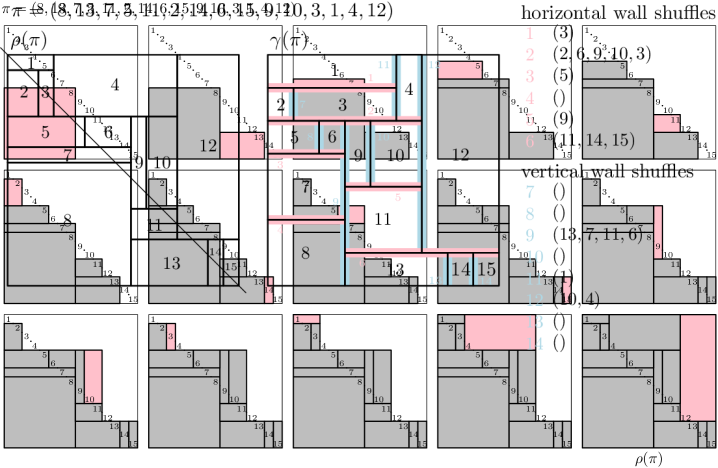
We are now in position to define the mapping , , from permutations to generic rectangulations; see Figure 21.From we first construct the diagonal rectangulation .Let be a horizontal wall in , and consider the rectangles in whose bottom side lies on from left to right.By construction of , these rectangles form an increasing subsequence of .Similarly, the rectangles in whose top side lies on from left to right form an increasing subsequence of .Thus, we can specify a wall shuffle by taking the subsequence of that contains the appropriate rectangle numbers.On the other hand, for a vertical wall in , the rectangles in whose left side lies on from bottom to top form a decreasing subsequence of , and the rectangles whose right side lies on form a decreasing subsequence of , so we can specify a wall shuffle by taking the subsequence of containing the appropriate rectangle numbers.The rectangulation is obtained from by applying wall slides to it, so as to obtain the wall shuffles specified by .
Lemma 25 ([Rea12, Prop. 4.2]).
The map is surjective.
Even though is not a bijection, Reading [Rea12] showed that it becomes a bijection when restricting the domain to 2-clumped permutations.
Theorem 26 ([Rea12, Thm. 4.1]).
The map is a bijection when restricted to the set of 2-clumped permutations.
8.5. The connection between permutations and rectangulations
The key lemma of this section, Lemma 28 below, asserts that deletion, insertion and jumps in permutations as defined in Section 8.2 are in bijective correspondence under to deletion, insertion and jumps in generic rectangulations as defined in Sections 2.3, 2.4 and 3.1.In order to prove it, we first establish a coarser version of this statement for the mapping .
Lemma 27.
Let , , and define .In the sequence , consider the subsequence consisting of the first insertion point of every vertical group, and the last insertion point of every horizontal group.Then we have for all , and the sequence can be partitioned into consecutive nonempty intervals with the following properties:
-
(a)
for every and every we have ;
-
(b)
for any interval , , such that the top-left vertex of in , , has type , we have that the rectangle is the unique rectangle left of , and the rectangle is the leftmost rectangle above ;
-
(c)
for any interval , , such that the top-left vertex of in , , has type , we have that the rectangle is the topmost rectangle left of , and the rectangle is the unique rectangle above ;
-
(d)
we have and .
Proof.
For the reader’s convenience, the proof is illustrated in Figure 22.Recall the definition of the mapping via the process described in Section 8.4 and illustrated in Figure 19.Using the definition of the rectangle insertion from Section 2.4, we first observe that and .We consider the sequence of permutations for and their images under .Observe that is obtained from by the adjacent transposition .We consider the construction of , specifically the two steps in which the rectangles and are added, and we analyze how the swapped insertion order of these two rectangles changes the resulting rectangulation .Clearly, in both and , the rectangle is either left-extended and top-fixed, or left-fixed and top-extended, and we treat both cases separately.In particular, these two cases are not symmetric.
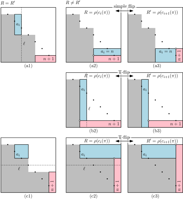
Case (i): is left-extended and top-fixed in .This case is shown in the top and middle part of Figure 22.We distinguish two subcases, namely and .Case (ia): .In this case the top side of coincides with the bottom side of in , as both rectangles left-extend to the same vertical line by the staircase property and the fact that every rectangle intersects the main diagonal; see Figure 22 (a2).Consequently, inserting them in the swapped order, first and then , produces a sub-rectangulation that differs in a simple flip of the wall between these two rectangles; see Figure 22 (a3).As the height of the top side of is not determined by , but only by previous rectangles , both insertion orders produce the same staircase , which by the definition of is all that matters for the next construction steps.Consequently, and differ in a simple flip of the rectangles and .Moreover, by the definition of rectangle deletion given in Section 2.3 we have , and by the definition of rectangle insertion and the definition of we have and for some index .Note that in , the top-left vertex of has type and , , is the leftmost rectangle above .Furthermore, in , the top-left vertex of has type and , , is the topmost rectangle left of .Case (ib): .If is bottom-fixed in , or if does not left-extend beyond the vertical line through the right endpoint of the th interval on the main diagonal, then the rectangles and do not touch; see Figure 22 (a1).Consequently, inserting them in the swapped order, first and then , produces the same sub-rectangulation.It follows that , i.e., , and therefore trivially .On the other hand, if is bottom-extended and left-extends beyond , then must be right-fixed because of (otherwise would reach into the st line segment on the main diagonal).Moreover, because of the staircase property the top side of contains the bottom side of , and both rectangles left-extend to the same vertical line; see Figure 22 (b2).Consequently, inserting them in the swapped order, first and then produces a sub-rectangulation that differs in a T-flip from to around the top-right common vertex of these two rectangles; see Figure 22 (b3).As the height of the top side of is not determined by , and as is right-fixed and is top-fixed in both insertion orders, we obtain that and differ in a T-flip around the top-right common vertex of the rectangles and .Moreover, by the definition of rectangle insertion and deletion and the definition of , we have , and and for some index .Note that in , the top-left vertex of has type and , , is the leftmost rectangle above .Furthermore, in , the top-left vertex of has type and , , is the unique rectangle left of .Case (ii): is left-fixed and top-extended in .This case is shown in the bottom part of Figure 22.As is top-extended, the staircase property implies that , as must be among the first entries of .If is right-fixed in , or if does not top-extend beyond the horizontal line through the right endpoint of the st interval on the main diagonal, then the rectangles and do not touch; see Figure 22 (c1).Consequently, inserting them in the swapped order, first and then , produces the same sub-rectangulation.It follows that , i.e., , and therefore trivially .On the other hand, if is right-extended and top-extends beyond , then must be bottom-fixed because of (otherwise would reach into the st line segment on the main diagonal).Moreover, because of the staircase property the top side of must lie on the horizontal line through the bottom side of , and therefore right-extends to the right outer boundary, i.e., the bottom side of contains the top side of ; see Figure 22 (c2).Consequently, inserting them in the swapped order, first and then produces a sub-rectangulation that differs in a T-flip from to around the bottom-left common vertex of these two rectangles; see Figure 22 (c3).As the height of the top side of is not determined by in the two insertion orders, we obtain that and differ in a T-flip around the bottom-left common vertex of the rectangles and .Moreover, by the definition of rectangle insertion and deletion and the definition of , we have , and and for some index .Note that in , the top-left vertex of has type and , , is the unique rectangle above .Furthermore, in , the top-left vertex of has type and , , is the topmost rectangle left of .This proves (a), (b) and (c).For (d) observe that the rectangle in the bottom-left corner of is , whereas the rectangle in the top-right corner is , so and .This completes the proof of the lemma.∎
Lemma 28.
Let , , and consider the rectangulation with insertion points.Then we have for all , and the sequence can be partitioned into consecutive nonempty intervals , such that for every and every we have .Furthermore, if is 2-clumped, then each interval contains exactly one 2-clumped permutation.
The proof of Lemma 28 shows that and .
Proof.
For any , consider the permutation , and the two diagonal rectangulations and .From Lemma 27 we know that and for some index such that the th insertion point in is the first of a vertical group, or the last of a horizontal group.By the definitions from Section 8.4, consists of applying plus wall slides that are determined by the wall shuffles of and and the relative order of the rectangle indices in those shuffles in and , i.e., and are obtained from and by wall slides.Observe that in and , the bottom-right rectangle is contained in at most one wall shuffle.Specifically, if the top-left corner of has type and does not lie on the left boundary of the rectangulation, then participates in a single wall shuffle of the vertical wall that contains the left side of , whereas if the top-left corner of has type and does not lie on the upper boundary of the rectangulation, then participates in a single wall shuffle of the horizontal wall that contains the top side of .In particular, in the cases and the rectangle is not contained in any wall shuffle.As the elements of all subsequences of and that do not contain appear in the same relative order in both permutations, all wall shuffles of and are the same, except the wall shuffle of containing , which is obtained from a wall shuffle of by inserting the value .We conclude that and for some index .The desired interval partition of the indices is obtained by refining the partition guaranteed by Lemma 27, where is the number of vertical and horizontal groups of , which is the same for , as wall slides do not affect it.As and by Lemma 27 (d), these two intervals are not refined, so we have and .It remains to consider the remaining intervals , .First consider an interval , , such that in , , the top-left vertex has type (recall Lemma 27 (a)).By Lemma 27 (b), in the rectangle is the unique rectangle left of , and the rectangle is the leftmost rectangle above .Consider the wall shuffle of the vertical wall between and in .It has the form , for some , i.e., the rectangles are stacked on top of and their bottom sides are incident with below the incidence of the top side of with .It follows that contains the subsequence , and so the permutations for have the value appear at every possible position within the subsequence .Consequently, the interval is refined into subintervals such that if are in the same subinterval and and for some index if are in consecutive subintervals.Now consider an interval , , such that in , , the top-left vertex has type (recall Lemma 27 (a)).By Lemma 27 (c), in the rectangle is the topmost rectangle left of , and the rectangle is the unique rectangle above .Consider the wall shuffle of the horizontal wall between and in .It has the form , for some , i.e., the rectangles are stacked to the left of and their right sides are incident with to the right of the incidence of the left side of with .It follows that contains the subsequence , and so the permutations for have the value appear at every possible position within the subsequence .Consequently, the interval is refined into subintervals such that if are in the same subinterval and and for some index if are in consecutive subintervals.It remains to argue that each set of permutations , , contains exactly one 2-clumped permutation.Indeed, can contain at most one 2-clumped permutation by Theorem 26, as all have the same image under .Suppose for the sake of contradiction that contains no 2-clumped permutation.Then by Theorem 26 there is another 2-clumped permutation with and for all .However, by Lemma 23, the permutation is also 2-clumped, i.e., we have .Moreover, we have as , and by Lemma 28 we have , a contradiction to the fact that is a bijection between and by Theorem 26.∎
8.6. Proof of Theorem 5
Proof of Theorem 5.
Consider a zigzag set of rectangulations , and consider the zigzag sets for .By Lemma 28, for all there is a set of 2-clumped permutations such that restricted to is a bijection between and , and such that for all .Moreover, as is a zigzag set, we know that for all we have and , for all .By Lemma 28, this implies that for all we have and , for all , i.e., is a zigzag language of 2-clumped permutations (using that and are zigzag languages).By Theorem 22, Algorithm J visits every permutation from exactly once, in the order defined by (2).From Lemma 24 (d) we obtain that if Algorithm J performs a jump of some value in the current permutation , then the corresponding rectangulations for are either bottom-based or right-based.Using the definition of jumps from Section 3.1 and Lemma 28, a minimal left/right jump of the value in , as performed by Algorithm J, corresponds to a minimal left/right jump of the rectangle in , as performed by Algorithm J□.This together with the observation that proves the first part of the theorem.Specifically, the ordering of rectangulations generated by Algorithm J□ is
| (3) |
To prove the second part of the theorem, by Theorem 22 it suffices to show that is even for all .For any rectangulation , we write for the rectangulation obtained by reflection at the main diagonal.First observe that if , , satisfy , then we also have .Consequently, the assumption that is symmetric implies that is symmetric for all .Consider a rectangulation , , and observe that if the top-left vertex of the bottom-right rectangle of has type , then it has type in , and vice versa.It follows that is an involution without fixed points on for all , proving that is even.This completes the proof.∎
8.7. Memoryless generation of permutations
Consider Algorithm M below, which takes as input a zigzag language of permutations and generates them exhaustively by minimal jumps in the same order as Algorithm J, i.e., in the order .Algorithm M (Memoryless minimal jumps).This algorithm generates all permutations of a zigzag language by minimal jumps in the same order as Algorithm J.It maintains the current permutation in the variable , and auxiliary arrays and .
-
M1.
[Initialize] Set , and , for .
-
M2.
[Visit] Visit the current permutation .
-
M3.
[Select value] Set , and terminate if .
-
M4.
[Jump value] In the current permutation , perform a jump of the value that is minimal w.r.t. , where the jump direction is left if and right if .
-
M5.
[Update and ] Set .If and is at the first position in or the value left of it is bigger than set , or if and is at the last position in or the value right of it is bigger than set , and in both cases set and . Go back to M2.
Theorem 29.
For any zigzag language of permutations , , Algorithm M visits every rectangulation from exactly once, in the order defined by (2).
The rest of this section is devoted to proving Theorem 29.For any in the sequence we define a sequence as follows:If we have with and we define .If , we consider the permutation in the sequence , and we define if appears at an odd position in , or if appears at an even position.If is not the last permutation in we define
| (4a) | |||||
| (4b) |
for , and if is the last permutation in we define
| (5a) | |||||
| (5b) | |||||
| (5c) |
for .The following lemma captures important properties of the sequences defined in this way.
Lemma 30.
The sequences defined in (4b) and (5c) have the following properties.
-
(a)
For the first permutation in the sequence , we have .
-
(b)
For any two consecutive permutations in the sequence , is obtained from by a jump of the value .
-
(c)
For the last permutation in we have .
Moreover, for any three consecutive permutations in we have:
-
(c)
If and differ in a jump of , and and differ in a jump of , then we have for .
-
(d)
If and differ in a jump of , and and differ in a jump of , then we have for and .
-
(e)
If and differ in a jump of , and differ in a jump of , and is not at a boundary position in , then we have for .
-
(f)
If and differ in a jump of , and differ in a jump of , and is at a boundary position in , then we have for , and .
Proof.
We prove these properties by induction on .The induction basis is trivial.For the induction step let and assume that all properties hold for the sequence .We first show the induction step for (a), (b) and (c).Consider a permutation in and define .To prove (a), let be the first permutation in (recall Lemma 24 (a)).We have and by induction and (a) we hence have .Using (4b) we obtain , as claimed.To prove (b), let be a permutation that is not the last in the sequence , and let be the permutation succeeding in .If is not the last permutation in the subsequence of , then by (2) the permutation is obtained from by a jump of the value , and then (b) follows directly from (4b).On the other hand, if is the last permutation in the subsequence , then is obtained from by a jump of the value by induction and (b), and by (5c) we have , as desired.To prove (c), let be the last permutation in .Then the permutation is also the last permutation in , so by induction we have .Using (5c) we see that , as desired.To prove (d), note that and therefore is not the last permutation in the subsequence , so the claim follows directly from (4a).To prove (e), note that and therefore is the last permutation in the subsequence , so the claim follows directly from (4a), (5a) and (5b).To prove (f) and (g), let , and .Note that and therefore is the last permutation in the subsequence , whereas is the first permutation in the subsequence .Consequently, is defined by (5c) and is defined by (4b).In particular, we have by (5b) and by (4a).We first prove (f), and we distinguish whether or .If , then and differ in a jump of , and as is not at a boundary position in , and also differ in a jump of by (2).Consequently, we have for by induction and (d), and by (4b), so (f) indeed holds in this case.If , then and differ in a jump of , and and differ in a jump of by (2).As is not at a boundary position in , we have for by induction and (f), and by induction and (b), so (f) indeed holds in this case.We now prove (g), and again we distinguish whether or .If , then and differ in a jump of , in particular , and as is at a boundary position in , and differ in a jump of some value smaller than by (2).Consequently, we have for and by induction and (e).Moreover, we have by (4a).Combining these observations shows that indeed (g) holds in this case.If , then and differ in a jump of , and and differ in a jump of by (2).Clearly, is at a boundary position in , and by induction and (g) we have for , and .Moreover, we have by (4a).Combining these observations proves (g) in this last case.∎
Proof of Theorem 29.
We establish the following invariants about the permutation visited in line M2 of the algorithm:
-
(A)
For all , the direction of the next jump of the value after the permutation in is left if and right if .
- (B)
By Lemma 24 (a), the identity permutation is the first permutation in the sequence .Moreover, by the initialization of in line M1, is also the first permutation visited in line M2.Combining this with the above invariants, we obtain by induction on the length of that after visiting a permutation , the next permutation visited by Algorithm M is the permutation that succeeds in .Indeed, by the instructions in line M3 and M4, the next permutation visited by the algorithm is obtained from by a jump of the value that is minimal w.r.t. , and the jump direction is left if and right if .Applying (B) and Lemma 30 (b), and (A) and Lemma 24 (c), we obtain that is indeed the permutation that succeeds in .Also, the algorithm terminates correctly after visiting the last permutation in the sequence by the condition in line M3 and Lemma 30 (c).We prove (A)+(B) by double induction on and the number of iterations of Algorithm M.The induction basis is trivial.For the induction step, let , and assume that the invariants hold for the zigzag language .We first verify that (A)+(B) hold in line M2 during the first iteration of the algorithm when .By line M1 we have for , so (A) is satisfied by Lemma 24 (b).By line M1 we also have , which equals by Lemma 30 (a).For the induction step, consider three consecutive permutations in the sequence , and suppose that (A)+(B) are satisfied when Algorithm M visits .We need to verify that (A)+(B) still hold after one iteration through lines M2—M5, after which the algorithm visits by the instructions in lines M3 and M4, as argued before.Case (i):We first consider the case that satisfy and therefore both are contained in the subsequence of .We only treat the case , as the other case is symmetric.In this case is obtained from by a left jump of the value .In particular, the variable has the value and in this iteration of the algorithm.Case (ia):The value is not at the first position in .Then by (2) the permutation is obtained from by another left jump of the value .In line M5, the value of is set to , which was the previous value, but none of the conditions in line M5 holds for , so overall none of the arrays and is modified.We conclude that (A) holds after this iteration for .Moreover, (B) holds by Lemma 30 (c) and (4b).Case (ib):The value is at the first position in , i.e., we have .Then by (2) we have where succeeds in the sequence .In line M5, the value of is set to , which is the same as the previous value, but since the first if-condition is satisfied, is then overwritten by , and is set to .Consequently, the new values are and by induction and (B) and (4a).Moreover, the value of is flipped to .Using Lemma 24 (e), we conclude that (A) holds after this iteration for .Applying Lemma 30 (d) and using that by (5c), we obtain that (B) holds as well.Case (ii):It remains to consider the case that , i.e., both permutations have at the first or last position.By symmetry, it suffices to consider the case that is at the first position, i.e., and , where and are consecutive permutations in .They differ in a jump of the value by Lemma 30 (b) and (B).Then by (2), the permutation is obtained from by a right jump of .We proceed to show that (A) and (B) hold for , and for this we distinguish subcases.Case (iia):The value is not at a boundary position in .Then by Lemma 24 (d) in the value is surrounded by the same values as in , both smaller than .In line M5, the value of is set to , and no other entries of and are modified.Using Lemma 24 (e), we conclude that (A) holds after this iteration for .Moreover, (B) holds by Lemma 30 (e), also using that by (4b).Case (iib):The value is at a boundary position in , and the value next to it is smaller than .Then by Lemma 24 (d) in the value is also next to , and either is at a boundary position (the right boundary, as is at the first position in ) or the other value next to in the direction of the jump is bigger than .In line M5, the value of is set to , the value of is set to , and is set to .Moreover, the value of is flipped.Using Lemma 24 (e), we conclude that (A) holds after this iteration for .Moreover, (B) holds by Lemma 30 (f), also using that by (4b).This completes the proof of the theorem.∎
8.8. Proof of Theorem 8
9. S-equivalence of rectangulations
Recall that R-equivalence is the equivalence relation on obtained from wall slides, i.e., any two generic rectangulations that differ in a sequence of wall slides are equivalent.It is well known that every equivalence class contains exactly one diagonal rectangulation, i.e., is a set of representatives for R-equivalence (see e.g. [CSS18]).
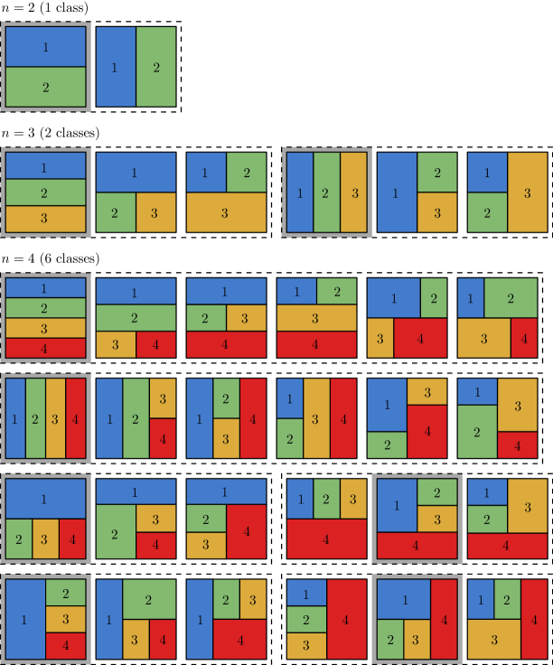
We aim to do something analogous for S-equivalence, and to pick a suitable set of representatives for our generation algorithm.Recall that S-equivalence is the equivalence relation on obtained from wall slides and simple flips, i.e., any two generic rectangulations that differ in a sequence of wall slides or simple flips are equivalent.Figure 23 shows the equivalence classes of generic rectangulations under S-equivalence for .Unfortunately, one can check that there is no choice of representatives , , for those equivalence classes (i.e., , , ) that is consistent with the operations of rectangle deletion and insertion, i.e., such that and .Consequently, for S-equivalence there is no set of unique representatives, one for each equivalence class, that would form a zigzag set, so our generation algorithms cannot be applied directly.However, we will show how to choose representatives for each equivalence class (highlighted in Figure 23), such that those representatives and the rectangulations obtained from them by a simple flip of the rectangle admit a generation tree approach with our algorithms.
9.1. Representatives for S-equivalence
By definition, S-equivalence is a coarsening of R-equivalence, and we will therefore choose a subset of diagonal rectangulations as representatives.We start with some definitions; see Figure 24.A rectangulation is horizontally aligned, or H-aligned for short, if all of its walls are horizontal.Moreover, a rectangulation is almost horizontally aligned, or AH-aligned for short, if all of its walls except one at the bottom are horizontal.Equivalently, it is obtained by gluing copies of on top of .Similarly, a rectangulation is vertically aligned, or V-aligned for short, if all of its walls are vertical.Moreover, a rectangulation is almost vertically aligned, or AV-aligned for short, if all of its walls except one at the right are vertical.Equivalently, it is obtained by gluing copies of on the left of .

The rectangulation is H-aligned and V-aligned.The rectangulation is H-aligned and AV-aligned, and the rectangulation is V-aligned and AH-aligned.A rectangulation is H- or V-alignable, if we can apply a sequence of simple flips to make it H- or V-aligned, respectively.Clearly, a rectangulation is H-alignable if it is obtained by vertically gluing together copies of and , and it is V-alignable if it is obtained by horizontally gluing together copies of and .A block in a rectangulation is a subset of rectangles whose union is a rectangle.The size of a block is the number of rectangles of the block.
Lemma 31.
Every diagonal rectangulation can be partitioned uniquely into maximal alignable blocks.
Proof.
Suppose for the sake of contradiction that for some rectangulation there were two distinct block partitions of .Consider a block in that is not a block in .Consider one of the rectangles in , and consider the block of containing this rectangle.As does not have any points where 4 rectangles meet and , the block must be a proper subset or superset of , contradicting the maximal choice of the blocks.∎
Lemma 31 holds more generally for generic rectangulations and for maximal blocks with any additional property (such as alignable), but this is not needed here.
Lemma 32.
For any diagonal rectangulation, the partition into maximal alignable blocks is invariant under simple flips.
Proof.
Consider a wall that can be simple-flipped, and observe that the two rectangles to both sides of the wall must belong to the same alignable block due to the maximal choice of the blocks.∎
From now on, whenever we refer to a block in a rectangulation, we mean a maximal alignable block.A block is a base block, if it contains the bottom boundary of the rectangulation.Based on the partition of a diagonal rectangulation into blocks, which is unique by Lemma 31, we introduce the following definitions; see Figure 25.We refer to each block of as an H-block or V-block, if it is H-alignable or V-alignable, respectively.We consider an H-block of size at least 2 with rectangle at the bottom-right.If or if rectangle of is below we say that is free, whereas if is right of we say that is locked.Similarly, we consider a V-block of size at least 2 with rectangle at the bottom-right.If or if rectangle of is right of we say that is free, whereas if is below we say that is locked.
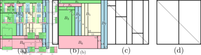
We say that is block-aligned if for every block of size at least 2 in the following conditions hold: if is a free H-block then is H-aligned, if is a free V-block then is V-aligned, if is a locked H-block then is AH-aligned, and if is a locked V-block then is AV-aligned.A special rule applies if the rectangle is contained in a block of size 2 (which is free and both H-alignable and V-alignable), and then we require this block to be V-aligned, unless it is a base block, in which case it must be H-aligned.Note that a block of size exactly 2 that does not contain is both an H-block and a V-block, however, if is a locked/free H-block then is a free/locked V-block, respectively, so this definition is consistent (as AH-aligned equals V-aligned and H-aligned equals AV-aligned for a block of size 2).We write for the set of diagonal rectangulations that are block-aligned.We partition this set into and , respectively, according to whether the rectangle is contained in a block of size 1 or at least 2, respectively.Note that if , then the wall between and does not admit a simple flip, whereas if , then this wall admits a simple flip.For any we write for the rectangulation obtained from by a simple flip of this wall.The set is partitioned into and according to whether this wall is horizontal or vertical, respectively.As a consequence of Lemma 32, every equivalence class of generic rectangulations under S-equivalence contains exactly one block-aligned diagonal rectangulation; see Figure 23.Consequently, we will use the block-aligned rectangulations as representatives for S-equivalence.
9.2. Insertion in block-aligned rectangulations
The next two lemmas describe how to construct block-aligned rectangulations by rectangle insertion; see Figure 27.For any diagonal rectangulation , we let denote the subsequence of of the first insertion point of each vertical group.Similarly, we let denote the subsequence of of the last insertion point of each horizontal group.
Lemma 33.
Let , and .Then we have the following:
-
•
For any we have , and every for which the top-left vertex of has type and forms its own block is obtained by insertion from some in this way.
-
•
For any we have , and every for which the top-left vertex of has type and forms its own block is obtained by insertion from some in this way.
-
•
If we have , and every for which and form a V-aligned block of size 2 is obtained by insertion from some in this way.
-
•
If we have , and every for which and form an H-aligned base block of size 2 is obtained by insertion from some in this way.
Proof.
The first and second part of the lemma are symmetric, so it suffices to prove the first one.For this we analyze how the blocks of differ from the blocks of , and prove that they are all aligned as required.The rectangle forms a block of size 1 in , and as this is also true in .Similarly, as the rectangle forms a block of size 1 in .Consequently, we only need to verify whether blocks of not containing or in are aligned as required.If , then the blocks of are the same as those of , plus the block containing , so we are done; see Figure 26 (a).If , we let and be the rectangles in to the left and right of the edge that contains the insertion point .If and belong to two distinct blocks in , then the blocks of are the same as those of , plus the block containing , so we are done; see Figure 26 (b).On the other hand, if and belong to the same block in , then it must be a free V-block that is V-aligned or a locked H-block that AH-aligned, and we have .If is a free V-block in , then in this block is split into two free V-blocks and , one containing and the other one containing , and both and are V-aligned; see Figure 26 (c).If is a locked H-block in , then in this block is split into the H-block , and two blocks of size 1 containing or , respectively; see Figure 26 (d).Moreover, if then , and otherwise is a free H-block that is H-aligned in .In all cases we obtain , as claimed.We continue to prove the third part of the lemma about the rectangulation .The rectangle forms a block of size 1 in , and together with it forms a block of size 2 in ; see Figure 26 (e).This block is V-aligned in , so we have , as claimed.It remains to prove the fourth part of the lemma about the rectangulation .The rectangle forms a block of size 1 in , and together with it forms a block of size 2 in ; see Figure 26 (f).This block is a base block and H-aligned in , so we have , as claimed.∎

Lemma 34.
Let and , or let and , and define and .Then we have the following:
-
•
For any we have , and every for which the top-left vertex of has type and is contained in a block of size at least 2 is obtained by insertion from some in this way.
-
•
For any we have , and every for which the top-left vertex of has type and is contained in a block of size at least 2 is obtained by insertion from some in this way.
-
•
We have , and every for which and are contained in an H-aligned block of size at least 3 is obtained by insertion from some in this way.
-
•
We have , and every for which and are contained in a V-aligned block of size at least 3 is obtained by insertion from some in this way.
Proof.
The proof for the first part in the case and for the second part in the case is analogous to the proof of Lemma 33.Therefore, by symmetry, to complete the proof of the first two parts, it suffices to argue about the case , and the rectangulation for ; see Figure 26 (g).The V-block in containing , which is free and V-aligned in , is AV-aligned and free in .Consequently, in the block is either split into two blocks, a free V-block that is V-aligned to the left of a locked V-block (Figure 26 (g1)) that is AV-aligned, or remains a single locked V-block that is AV-aligned in (Figure 26 (g2)), where the locking is due to the insertion of .The remaining blocks of are treated as in the proof of Lemma 33.In all cases we obtain that , as claimed.The third and fourth part of the lemma are symmetric, so it suffices to prove the third one about the rectangulation .In this case is an H-block that is free and H-aligned in , and either or is a V-block that is free and V-aligned in ; see Figure 26 (h).It follows that , as claimed.∎
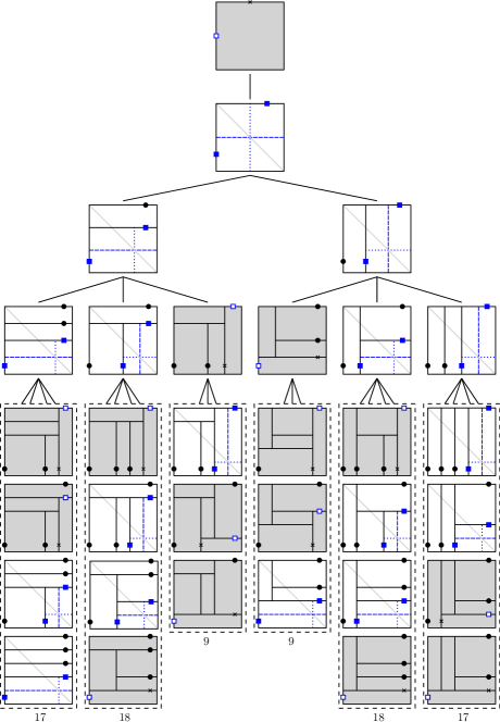
9.3. Tree of block-aligned rectangulations
By Lemmas 33 and 34, all block-aligned rectangulations can be obtained by suitable rectangle insertions into all block-aligned rectangulations and .We consider the subtree of the tree of rectangulations discussed in Section 3.4 induced by the rectangulations and for all .By gluing together pairs of nodes for all , we obtain the tree shown in Figure 27.For any , using the notation from Lemma 33 we define
| (6a) | |||
| For any and , using the notation from Lemma 34 we define | |||
| (6b) | |||
These sequences define an ordering among the children of each node in the aforementioned (unordered) tree of block-aligned rectangulations.Note that any two consecutive rectangulations in the sequence (6a) differ in a T-flip, except and , and and , which differ in a T-flip plus a simple flip.Similarly, any two consecutive rectangulations in the sequence (6b) differ in a T-flip, except and , which differ in a simultaneous flip of the two walls between , and .We refer to this operation as a D-flip (D like ‘double’).
9.4. Next oracle for block-aligned rectangulations
Using (6), we may modify the minimal jump oracle for diagonal rectangulations described in Section 7.2 for the generation of block-aligned rectangulations within Algorithm M□ as follows.Some Gray code orderings produced by this algorithm are shown in the appendix. (Next oracle for block-aligned rectangulations).
-
N1.
[Prepare] Set and call .If and , set and .If goto N2, otherwise we have and goto N3.If and , set and goto N4.If and , set and .If goto N5, otherwise we have and goto N6.If and , set and goto N7.
-
N2.
[Horizontal left jump (T/TS)] Set and call .Then set , , , , , and if and [ or [ and ]] call .Call and return.
-
N3.
[Horizontal left jump (ST/D)] Set and and call .Then set , , and and call .Set , and .If we have , set , and call .Call and return.
-
N4.
[Horizontal right jump (T/TS)] Set , and and call .Then set , , , , , and , and if and we have , set and call .Call and return.
-
N5.
[Vertical right jump (T/TS)] Set and call .Then set , , , , , , and if and [ or [ and not [ and ]] call .Call and return.
-
N6.
[Vertical right jump (ST/D)] Set and and call .Then set , , and and call .Set , and .If we have , set , and call .Call and return.
-
N7.
[Vertical left jump (T/TS)] Set , and and call .Then set , , , , , and , and if and we have , set and call .Call and return.
Lines N2–N4 are symmetric to lines N5–N7, so we only consider N2–N4; see the illustrations in Figure 28.Lines N2 and N4 perform a T-flip, possibly followed by a simple flip.Line N3 performs a simple flip followed by a T-flip, possibly followed by a simple flip, and in this case the combination of three flips, simple flip plus T-flip plus simple flip, yields a D-flip overall.The function , , called at the end of each of the lines N2–N7 checks whether rectangle participates in an H-aligned block (if ) or V-aligned block (if ) that is locked and must be transformed to an AH-aligned block or AV-aligned block by a simple flip.The function , , called at the beginning in line N1 does the converse, namely checking whether participates in an AH-aligned block or AV-aligned block that must be made H-aligned or V-aligned, respectively, before performing a jump of rectangle in direction .The implementation of these functions is shown below for the cases and .The other variants and are omitted for simplicity.

(Lock block if necessary).
-
L1.
[Prepare] Set , , , , and return if or or .
-
L2.
[Lock if necessary] Set and if call .
(Unlock block if necessary).
-
U1.
[Prepare] Set , , and .
-
U2.
[Unlock if necessary] If and call .
To use Algorithm M□ with this oracle, in line M5 we also need to check whether is bottom-based or right-based (in addition to ), and whether or are one simple flip away from such a configuration.Similarly, to use this oracle in conjunction with the oracle defined in Section 7.3, we need to test containment of a pattern in the rectangulation after a jump of rectangle not only via , but also using and , as all three rectangles , and may be modified through one call of .For details see our C++ implementation [cos].We obtain the following analogue of Theorems 7 and 8.
Theorem 35.
Let .For any set of patterns that are neither bottom-based nor right-based nor simple-flippable to a bottom-based or right-based pattern, Algorithm M□ with the oracle defined in Section 7.3, which calls as defined above, visits every rectangulation from exactly once, performing a sequence of one T- or D-flip plus at most three simple flips in each step.
It remains to analyze the running time of this algorithm.
Lemma 36.
Each call takes time .
As we are dealing with a subset of diagonal rectangulations, the proof is very similar to the proof of Lemma 14.
Proof.
Consider any of the calls , , in lines N2–N7 and let be the rectangulation after the call.As we only consider the first insertion point of each vertical group and the last insertion point of each horizontal group of , we have and , so the claim follows from Lemma 10 (b)+(c).∎
Lemma 36 immediately yields the following result.
Theorem 37.
Algorithm M□ with the oracle takes time to visit each block-aligned rectangulation.
For the pattern avoidance version of this algorithm, we obtain the following runtime bounds.
Theorem 38.
For any set of patterns , Algorithm M□ with the oracle visits each rectangulation from in time .
10. Counting pattern-avoiding rectangulations
In this section we report on computer experiments that count pattern-avoiding rectangulations for all interesting subsets of patterns where , , , , , , , .Clearly, we can omit sets of patterns that are equivalent to another set of patterns under actions (rotations and mirroring vertically or horizontally).Table 3 shows the results for generic rectangulations as a base class, and Table 4 for block-aligned rectangulations as a base class.The set of patterns used in each row of the table is denoted by the pattern indices, omitting curly brackets and commas.For example, the row 1478 refers to the set .When counting block-aligned rectangulations with our algorithms, the patterns cannot be used, as they do not satisfy the conditions of Theorem 35.
| Patterns | Counts for | OEIS | ||||||||||||
|---|---|---|---|---|---|---|---|---|---|---|---|---|---|---|
| A342141 | ||||||||||||||
| 1 | ||||||||||||||
| 3 | A117106 ? | |||||||||||||
| 7 | ||||||||||||||
| 12 | ||||||||||||||
| 13 | ||||||||||||||
| 14 | ||||||||||||||
| 17 | ||||||||||||||
| 34 | A001181 | |||||||||||||
| 35 | ||||||||||||||
| 36 | A001181 ? | |||||||||||||
| 37 | ||||||||||||||
| 38 | ||||||||||||||
| 78 | ||||||||||||||
| 123 | ||||||||||||||
| 127 | ||||||||||||||
| 134 | A000139 ? | |||||||||||||
| 135 | ||||||||||||||
| 136 | A000139 ? | |||||||||||||
| 137 | ||||||||||||||
| 138 | ||||||||||||||
| 145 | A000139 ? | |||||||||||||
| 147 | ||||||||||||||
| 148 | ||||||||||||||
| 178 | ||||||||||||||
| 345 | A281784 ? | |||||||||||||
| 347 | ||||||||||||||
| 357 | ||||||||||||||
| 358 | ||||||||||||||
| 367 | ||||||||||||||
| 378 | ||||||||||||||
| 1234 | A006318 | |||||||||||||
| 1235 | ||||||||||||||
| 1236 | A006318 ? | |||||||||||||
| 1237 | ||||||||||||||
| 1238 | ||||||||||||||
| 1278 | ||||||||||||||
| 1345 | ||||||||||||||
| 1346 | ||||||||||||||
| 1347 | ||||||||||||||
| 1348 | ||||||||||||||
| 1357 | ||||||||||||||
| 1358 | ||||||||||||||
| 1367 | ||||||||||||||
| 1378 | ||||||||||||||
| 1457 | ||||||||||||||
| 1478 | ||||||||||||||
| 3456 | ||||||||||||||
| 3457 | ||||||||||||||
| 3458 | ||||||||||||||
| 3478 | ||||||||||||||
| 3578 | ||||||||||||||
| 3678 | ||||||||||||||
| 12345 | A106228 ? | |||||||||||||
| 12347 | ||||||||||||||
| 12357 | ||||||||||||||
| 12358 | ||||||||||||||
| 12367 | ||||||||||||||
| 12378 | ||||||||||||||
| 13456 | ||||||||||||||
| 13457 | ||||||||||||||
| 13458 | ||||||||||||||
| 13467 | ||||||||||||||
| 13468 | ||||||||||||||
| 13478 | ||||||||||||||
| 13578 | ||||||||||||||
| 13678 | ||||||||||||||
| 14578 | ||||||||||||||
| 34567 | ||||||||||||||
| 34578 | ||||||||||||||
| 123456 | A078482 | |||||||||||||
| 123457 | A033321 ? | |||||||||||||
| 123458 | ||||||||||||||
| 123478 | ||||||||||||||
| 123578 | ||||||||||||||
| 123678 | ||||||||||||||
| 134567 | ||||||||||||||
| 134578 | ||||||||||||||
| 134678 | ||||||||||||||
| 345678 | A000984 ? | |||||||||||||
| 1234567 | ||||||||||||||
| 1234578 | ||||||||||||||
| 1345678 | A026029 ? | |||||||||||||
| 12345678 | A006012 | |||||||||||||
| Patterns | Counts for | OEIS | |||||||||||||
| A214358 | |||||||||||||||
| 1 | |||||||||||||||
| 12 | A078482 | ||||||||||||||
Several of these counting sequences appear in the OEIS [oei20], and are related to pattern-avoiding permutations (see e.g. [BGRR18]).The matching OEIS entries marked with ? are observed through are numerical experiments, but no formal bijective proof has been obtained yet, even though finding one should be straightforward in some cases.The last two rows in Table 3 with ? are interesting, as the correspondence to the objects mentioned in those OEIS entries is not obvious.This is true in particular for OEIS sequence A000984, which are the central binomial coefficients .
11. Open questions
The subject of pattern-avoiding rectangulations deserves further systematic investigation, and may still hold many undiscovered gems; recall Table 3.Understanding the number of pattern-avoiding rectangulations that are obtained by rectangle insertion may also help to improve the runtime bounds for our generation algorithms (recall Remark 21).Moreover, does the avoidance of a rectangulation pattern always correspond to the avoidance of a particular permutation pattern, and what is this correspondence?In our paper we considered R-equivalence and S-equivalence of generic rectangulations , and these equivalence relations are induced by wall slides, or by wall slides and simple flips, respectively.Considering all three basic flip operations , namely wall slides, simple flips, and T-flips, there are possible subsets of to induce an equivalence relation on .Which of these equivalence relations are interesting (apart from , and considered here), and what are suitable representatives that can be generated efficiently?Another interesting question to investigate would be Gray codes for rectangulations of point sets as introduced by Ackerman, Barequet and Pinter [ABP06b].Some first results in this direction have been obtained by Yamanaka, Rahman and Nakano [YRN18].In particular, can we apply our permutation-based generation framework for this task?
Acknowledgements
We thankfully acknowledge several discussions in the early phases of this manuscript with Hung P. Hoang, which took place at the 17th Gremo Workshop on Open Problems in Switzerland.We thank the organizers for the invitation to the workshop, and the other participants for the pleasant and stimulating working atmosphere.Furthermore, we thank the reviewers for their numerous helpful comments, which helped improving the manuscript.
References
- [ABBM+13] A. Asinowski, G. Barequet, M. Bousquet-Mélou, T. Mansour, and R. Y. Pinter. Orders induced by segments in floorplans and (2-14-3,3-41-2)-avoiding permutations. Electron. J. Combin., 20(2):Paper 35, 43, 2013.
- [ABP06a] E. Ackerman, G. Barequet, and R. Y. Pinter. A bijection between permutations and floorplans, and itsapplications. Discrete Appl. Math., 154(12):1674–1684, 2006.
- [ABP06b] E. Ackerman, G. Barequet, and R. Y. Pinter. On the number of rectangulations of a planar point set. J. Combin. Theory Ser. A, 113(6):1072–1091, 2006.
- [AF96] D. Avis and K. Fukuda. Reverse search for enumeration. Discrete Appl. Math., 65(1-3):21–46, 1996. First International Colloquium on Graphs and Optimization (GOI), 1992(Grimentz).
- [AM10] A. Asinowski and T. Mansour. Separable -permutations and guillotine partitions. Ann. Comb., 14(1):17–43, 2010.
- [ANY07] K. Amano, S. Nakano, and K. Yamanaka. On the number of rectangular drawings: Exact counting and lower andupper bounds. IPSJ SIG Technical Report 2007-AL-115 (5), 2007.
- [BER76] J. R. Bitner, G. Ehrlich, and E. M. Reingold. Efficient generation of the binary reflected Gray code and itsapplications. Comm. ACM, 19(9):517–521, 1976.
- [BGRR18] M. Bouvel, V. Guerrini, A. Rechnitzer, and S. Rinaldi. Semi-Baxter and strong-Baxter: two relatives of the Baxtersequence. SIAM J. Discrete Math., 32(4):2795–2819, 2018.
- [CM14] J. Conant and T. Michaels. On the number of tilings of a square by rectangles. Ann. Comb., 18(1):21–34, 2014.
- [cos] The Combinatorial Object Server: Generate rectangulations.http://www.combos.org/rect.
- [CSS18] J. Cardinal, V. Sacristán, and R. I. Silveira. A note on flips in diagonal rectangulations. Discrete Math. Theor. Comput. Sci., 20(2):Paper No. 14, 22,2018.
- [Ehr73] G. Ehrlich. Loopless algorithms for generating permutations, combinations, andother combinatorial configurations. J. Assoc. Comput. Mach., 20:500–513, 1973.
- [EMSV12] D. Eppstein, E. Mumford, B. Speckmann, and K. Verbeek. Area-universal and constrained rectangular layouts. SIAM J. Comput., 41(3):537–564, 2012.
- [Fel13] S. Felsner. Rectangle and square representations of planar graphs. In Thirty essays on geometric graph theory, pages 213–248.Springer, New York, 2013.
- [FFNO11] S. Felsner, É. Fusy, M. Noy, and D. Orden. Bijections for Baxter families and related objects. J. Combin. Theory Ser. A, 118(3):993–1020, 2011.
- [FIT09] R. Fujimaki, Y. Inoue, and T. Takahashi. An asymptotic estimate of the numbers of rectangular drawings orfloorplans. In 2009 IEEE International Symposium on Circuits and Systems(ISCAS), pages 856–859, 2009.
- [FNT21] S. Felsner, A. Nathenson, and C. D. Tóth. Aspect ratio universal rectangular layouts. Manuscript, 2021.
- [Fus09] É. Fusy. Transversal structures on triangulations: a combinatorial study andstraight-line drawings. Discrete Math., 309(7):1870–1894, 2009.
- [He14] B. D. He. A simple optimal binary representation of mosaic floorplans andBaxter permutations. Theoret. Comput. Sci., 532:40–50, 2014.
- [HHC+00] X. Hong, G. Huang, Y. Cai, J. Gu, S. Dong, C.-K. Cheng, and J. Gu. Corner block list: An effective and efficient topologicalrepresentation of non-slicing floorplan. In E. Sentovich, editor, Proceedings of the 2000 IEEE/ACMInternational Conference on Computer-Aided Design, 2000, San Jose,California, USA, November 5-9, 2000, pages 8–12. IEEE Computer Society,2000.
- [HHMW20] E. Hartung, H. P. Hoang, T. Mütze, and A. Williams. Combinatorial generation via permutation languages. In Shuchi Chawla, editor, Proceedings of the 2020 ACM-SIAMSymposium on Discrete Algorithms, SODA 2020, Salt Lake City, UT, USA,January 5-8, 2020, pages 1214–1225. SIAM, 2020.
- [HHMW21] E. Hartung, H. P. Hoang, T. Mütze, and A. Williams. Combinatorial generation via permutation languages. I.Fundamentals. To appear in Trans. Amer. Math. Soc.; preprint available athttps://arxiv.org/abs/1906.06069, 2021.
- [HM21] H. P. Hoang and T. Mütze. Combinatorial generation via permutation languages. II. Latticecongruences. To appear in Israel J. Math.; preprint available athttps://arxiv.org/abs/1911.12078, 2021.
- [ITF09] Y. Inoue, T. Takahashi, and R. Fujimaki. Counting rectangular drawings or floorplans in polynomial time. IEICE Trans. Fundam. Electron. Commun. Comput. Sci.,92-A(4):1115–1120, 2009.
- [KH97] G. Kant and X. He. Regular edge labeling of -connected plane graphs and itsapplications in graph drawing problems. Theoret. Comput. Sci., 172(1-2):175–193, 1997.
- [Knu11] D. E. Knuth. The Art of Computer Programming. Vol. 4A. Combinatorialalgorithms. Part 1. Addison-Wesley, Upper Saddle River, NJ, 2011.
- [Lei21] L. J. Leifheit. Combinatorial properties of rectangulations. Master’s thesis, TU Berlin, 2021.
- [LR12] S. Law and N. Reading. The Hopf algebra of diagonal rectangulations. J. Combin. Theory Ser. A, 119(3):788–824, 2012.
- [Mee19] E. Meehan. The Hopf algebra of generic rectangulations. https://arxiv.org/abs/1903.09874, 2019.
- [MSL76] W. J. Mitchell, J. P. Steadman, and R. S. Liggett. Synthesis and optimization of small rectangular floor plans. Environment and Planning B: Planning and Design, 3(1):37–70,1976.
- [Nak01] S. Nakano. Enumerating floorplans with rooms. In Algorithms and computation (Christchurch, 2001), volume2223 of Lecture Notes in Comput. Sci., pages 107–115. Springer,Berlin, 2001.
- [oei20] OEIS Foundation Inc. The on-line encyclopedia of integer sequences,2020. http://oeis.org.
- [Ott82] R. H. J. M. Otten. Automatic floorplan design. In J. S. Crabbe, C. E. Radke, and H. Ofek, editors, Proceedingsof the 19th Design Automation Conference, DAC ’82, Las Vegas, Nevada, USA,June 14-16, 1982, pages 261–267. ACM/IEEE, 1982.
- [PPR21] A. Padrol, V. Pilaud, and J. Ritter. Shard polytopes. To appear in Proceedings of the 33rd International Conference onFormal Power Series and Algebraic Combinatorics; preprint available athttps://arxiv.org/abs/2007.01008, 2021.
- [PS19] V. Pilaud and F. Santos. Quotientopes. Bull. Lond. Math. Soc., 51(3):406–420, 2019.
- [Rea12] N. Reading. Generic rectangulations. European J. Combin., 33(4):610–623, 2012.
- [Rus16] F. Ruskey. Combinatorial Gray code. In M.-Y. Kao, editor, Encyclopedia of Algorithms, pages342–347. Springer, 2016.
- [Sav97] C. Savage. A survey of combinatorial Gray codes. SIAM Rev., 39(4):605–629, 1997.
- [SC03] Z. C. Shen and C. C. N. Chu. Bounds on the number of slicing, mosaic, and general floorplans. IEEE Transactions on Computer-Aided Design of IntegratedCircuits and Systems, 22(10):1354–1361, 2003.
- [TN04] M. Takagi and S. Nakano. Listing all rectangular drawings with certain properties. Systems and Computers in Japan, 35(4):1–8, 2004.
- [vKS07] M. van Kreveld and B. Speckmann. On rectangular cartograms. Comput. Geom., 37(3):175–187, 2007.
- [Wil13] A. Williams. The greedy Gray code algorithm. In Algorithms and Data Structures - 13th InternationalSymposium, WADS 2013, London, ON, Canada, August 12-14, 2013. Proceedings,pages 525–536, 2013.
- [YCCG03] B. Yao, H. Chen, C.-K. Cheng, and R. L. Graham. Floorplan representations: Complexity and connections. ACM Trans. Design Autom. Electr. Syst., 8(1):55–80, 2003.
- [YCYN06] S. Yoshii, D. Chigira, K. Yamanaka, and S. Nakano. Constant time generation of rectangular drawings with exactlyn faces. IEICE Trans. Fundam. Electron. Commun. Comput. Sci.,89-A(9):2445–2450, 2006.
- [YRN18] K. Yamanaka, M. S. Rahman, and S. Nakano. Enumerating floorplans with columns. IEICE Trans. Fundam. Electron. Commun. Comput. Sci.,101-A(9):1392–1397, 2018.
Appendix A Visualization of Gray codes
In this section we visualize the Gray codes obtained from our algorithms for generic rectangulations, diagonal rectangulations and block-aligned rectangulations (without any forbidden patterns).The corresponding 2-clumped permutations are shown below each rectangulation.
A.1. Generic rectangulations
| 1 |
| 12 | 21 |
| 123 | 132 | 312 | 321 | 231 | 213 |
| 1234 | 1243 | 1423 | 4123 | 4132 | 1432 | 1342 | 1324 | 3124 | 3142 | 3412 |
|---|---|---|---|---|---|---|---|---|---|---|
| 4312 | 4321 | 3421 | 3241 | 3214 | 2314 | 2341 | 2431 | 4231 | 4213 | 2413 |
| 2143 | 2134 |
| 12345 | 12354 | 12534 | 15234 | 51234 | 51243 | 15243 | 12543 | 12453 |
| 12435 | 14235 | 14253 | 14523 | 15423 | 51423 | 54123 | 45123 | 41523 |
| 41253 | 41235 | 41325 | 41352* | 41532 | 45132 | 54132 | 51432 | 15432 |
| 14532 | 14352 | 14325 | 13425 | 13452 | 13542 | 15342 | 51342 | 51324 |
| 15324 | 13524 | 13254 | 13245 | 31245 | 31254 | 31524 | 53124 | 53142 |
| 31542 | 31452 | 31425 | 34125 | 34152 | 34512 | 35412 | 53412 | 54312 |
| 45312 | 43512 | 43152 | 43125 | 43215 | 43251 | 43521 | 45321 | 54321 |
| 53421 | 35421 | 34521 | 34251 | 34215 | 32415 | 32451 | 32541 | 35241 |
| 53241 | 53214 | 35214 | 32514 | 32154 | 32145 | 23145 | 23154 | 23514 |
| 25314* | 52314 | 52341 | 25341 | 23541 | 23451 | 23415 | 24315 | 24351 |
| 24531 | 25431 | 52431 | 54231 | 45231 | 42531 | 42351 | 42315 | 42135 |
| 42153 | 45213 | 54213 | 52413 | 25413 | 24153 | 24135 | 21435 | 21453 |
| 21543 | 25143 | 52143 | 52134 | 25134 | 21534 | 21354 | 21345 |
A.2. Diagonal rectangulations
| 1 |
| 12 | 21 |
| 123 | 132 | 312 | 321 | 231 | 213 |
| 1234 | 1243 | 1423 | 4123 | 4132 | 1432 | 1342 | 1324 | 3124 | 3142 | 4312 |
| 4321 | 3421 | 3241 | 3214 | 2314 | 2341 | 2431 | 4231 | 4213 | 2413 | 2134 |
| 12345 | 12354 | 12534 | 15234 | 51234 | 51243 | 15243 | 12543 | 12453 |
|---|---|---|---|---|---|---|---|---|
| 12435 | 14235 | 14253 | 15423 | 51423 | 54123 | 41253 | 41235 | 41325 |
| 41352* | 41532 | 54132 | 51432 | 15432 | 14532 | 14352 | 14325 | 13425 |
| 13452 | 13542 | 15342 | 51342 | 51324 | 15324 | 13524 | 13245 | 31245 |
| 31524 | 53124 | 53142 | 31542 | 31452 | 31425 | 43125 | 43152 | 45312 |
| 54312 | 54321 | 45321 | 43521 | 43251 | 43215 | 34215 | 34251 | 34521 |
| 35421 | 53421 | 53241 | 35241 | 32451 | 32415 | 32145 | 35214 | 53214 |
| 52314 | 25314* | 23514 | 23145 | 23415 | 23451 | 23541 | 25341 | 52341 |
| 52431 | 25431 | 24531 | 24351 | 24315 | 42315 | 42351 | 42531 | 54231 |
| 54213 | 42153 | 42135 | 24135 | 24153 | 25413 | 52413 | 52134 | 25134 |
| 21354 | 21345 |
A.3. Block-aligned rectangulations
| 1 |
| 21 |
| 123 | 321 |
| 1234 | 1432 | 4132 | 4321 | 2341 | 2314 |
| 12345 | 12543 | 15243 | 51243 | 51432 | 15432 | 13452 | 13425 | 41325 |
|---|---|---|---|---|---|---|---|---|
| 41352* | 54132 | 54321 | 34521 | 34251 | 34215 | 23415 | 23451 | 25431 |
| 52431 | 52314 | 25314* | 23145 |