Graph Convolutional Network for Swahili News Classification

Abstract

This work empirically demonstrates the ability of Text Graph Convolutional Network (Text GCN) to outperform traditional natural language processing benchmarks for the task of semi-supervised Swahili news classification. In particular, we focus our experimentation on the sparsely-labelled semi-supervised context which is representative of the practical constraints facing low-resourced African languages. We follow up on this result by introducing a variant of the Text GCN model which utilises a bag of words embedding rather than a naive one-hot encoding to reduce the memory footprint of Text GCN whilst demonstrating similar predictive performance.

1 Introduction

Text classification is a widespread natural language processing (NLP) task with applications including topic classification Wang and Manning (2012), content moderation Bodapati et al. (2019), and fake news detection Wang (2017). News categorisation, another example application, is of particular relevance as it is used to automatically handle the incredible volume of news published daily. Effective classification assists in better article recommendation for readers, semantic topic categorisation, and removal of abusive or untrue content Minaee et al. (2020).

Traditional news classification techniques involve extracting features from the text followed by a classifier to generate predictions. More recently, large transformer-based pre-trained models have dominated text classification benchmarks in high-resource settings Yang et al. (2019); Sun et al. (2020).

Graph Neural Networks (GNNs), a family of model architectures designed to operate directly on irregularly structured graphs, have seen a recent uptick in popularity in several applications. These include citation networks Fey et al. (2018); Veličković et al. (2018); Kipf and Welling (2017), semantic role labelling Marcheggiani and Titov (2017), machine translation Beck et al. (2018), and named entity recognition Cetoli et al. (2017). Although news texts superficially present a sequence of words, a document contains an implicit graph structure in the form of semantic and syntactic relationships Mihalcea and Tarau (2004). A corpus can be arranged into a graph by making use of both inter-document and intra-document relationships. Yao et al. (2019) construct a single graph from the complete corpus while Huang et al. (2019) construct a graph on a per-document basis.

2 Motivation

Despite the importance of this application area and Swahili being the fourteenth most widely spoken language in the world Eberhard et al. (2020), there is a deficit of published work on text classification for Swahili documents. Some of the factors contributing to this under-representation include a shortage of freely-available annotated datasets, and limited literature comparing methods commonly applied to high-resource languages in a low-resource context Orife et al. (2020); Niyongabo et al. (2020). Joshi et al. (2020) classify Swahili as a hopeful language, indicating that although research endeavours and community-driven efforts to digitise and annotate data exist Hurskainen and Department of World Cultures, University of Helsinki (2016); David (2020); Shikali and Mokhosi (2020), there remains a sizeable gap between the NLP tools available for Swahili and high-resource languages.

Off the back of the effectiveness of transformer-based models in high-resource settings, efforts have been made to apply these architectures to low-resource languages. While multilingual models Lample and Conneau (2019); Conneau et al. (2020) have shown promising zero-shot cross-lingual results, the performance has been shown to vary greatly by target languages, often with a large drop for tasks in low-resource languages like Swahili Jiang et al. (2020); Hu et al. (2020). An alternative approach, with comparable results, involves transferring monolingual models to a target language Tran (2020); Artetxe et al. (2020). This method still relies on sequentially fine-tuning transformer models, which has financial and ethical implications Strubell et al. (2019). In addition to these shortcomings, transformer-based methods typically impose a memory requirement which scales quadratically with the sequence length. Despite work to reduce this drawback Zaheer et al. (2021); Beltagy et al. (2020), large transformer-based models remain computationally challenging in the context of African research and industry.

Consequently, we aim to combat these challenges with the following set of contributions:

• Provide a set of accessible traditional NLP benchmarks for Swahili news classification.

• Empirically compare these benchmarks to a Text Graph Convolutional Network (Text GCN) solution which was initially developed for English. To our knowledge this is the first instance of a GNN being used for text classification on any African language dataset.

• Focus experiments on the semi-supervised context where the number of labels are highly constrained and the compute is restricted.

3 Graph Neural Networks

Graph Neural Networks are a neural network model architecture which is able to generalise to non-euclidean data structures Gori et al. (2005); Scarselli et al. (2009); Battaglia et al. (2018). As with other modern deep learning architectures, a GNN is constructed by stacking a number of GNN layers sequentially. In fact, Wu et al. (2021) and Zhou et al. (2018) present GNNs as a generalisation of convolutional neural networks. The underlying idea is that for a given graph $\mathcal{G}$, with nodes $\mathcal{V}$ and edges $\mathcal{E}$, one can learn a rich representation for each input node by aggregating information from its neighbourhood. Each node $v_{i}$ is initially represented by an embedding vector $x_{i}\in\mathbb{R}^{F}$ while the edge structure is stored in an adjacency matrix $A\in\mathcal{R}^{N\times N}$. $N$ is the number of nodes in $\mathcal{G}$. By stacking GNN layers, one can learn increasingly rich representations by incorporating features from neighbours of neighbours. Figure 1 illustrates how the hidden representation of $h_{i}\in\mathcal{R}^{F^{\prime}}$ is obtained by aggregating the 1-hop neighbourhood along the red shaded edges.

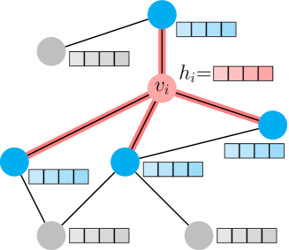
Figure 1: Information is pooled along the shaded edges in the graph and aggregated at node $v_{i}$ to update the hidden representation of $h_{i}$.

3.1 Text Graph Convolutional Networks

Graph Convolutional Networks (GCNs), a particular type of GNN, aim to learn a localised and fast approximation of a spectral graph convolution Kipf and Welling (2017). A GCN layer can be formalised mathematically as given in equation 1 where $H^{(\ell)}\in\mathbb{R}^{N\times F}$ is the node representation at layer $\ell$, $\Theta^{(\ell)}\in\mathbb{R}^{F\times F^{\prime}}$ are trainable parameters, and $\phi(\cdot)$ is an element-wise activation function. The $\widetilde{D}^{-\frac{1}{2}}\widetilde{A}\widetilde{D}^{-\frac{1}{2}}$ term is the result of the renormalisation trick wherein $\widetilde{A}=A+\mathbb{1}_{N}$ and $\widetilde{D}_{ii}=\sum_{j}\widetilde{A}_{ij}$.

$$H^{(\ell+1)}=\phi\left(\widetilde{D}^{-\frac{1}{2}}\widetilde{A}\widetilde{D}^{-\frac{1}{2}}H^{(\ell)}\Theta^{(\ell)}\right)$$ (1)

In semi-supervised classification, a GCN is trained using gradient descent where the loss is calculated using cross entropy over the subset of labelled nodes. Unlike many self-training approaches, which rely on sudo-labels generated by a supervised model trained on the labelled subset of the data Jo and Cinarel (2019), a GCN operates directly on all nodes and without the need to generate potentially noisy sudo-labels.

Text GCN applies this model to a corpus of documents by treating documents and words as nodes in a heterogeneous graph Yao et al. (2019). Furthermore, Text GCN constructs a weighted adjacency matrix by representing document-word interactions using their TF-IDF value and word-word interactions using Positive Point-wise Mutual Information (PPMI) over a fixed length context window (see Appendix A).

4 Experiments

All experiments presented below are conducted in a transductive setting and assume a fixed corpus size. Furthermore, results are presented in terms of the mean and standard deviation obtained by repeating all experiments 5 times with different seeds.

4.1 Data

The Swahili News Classification dataset David (2020) is used to compare the ability of each model to categorise news articles into one of six categories: kitaifa (“national”), michezo (“sports”), burudani (“entertainment”), uchumi (“economy”), kimataifa (“international”), and afya (“health”). In total, the data contains 23,266 labelled samples which we divide into train, validation, and test sets using a 8:1:1 split. Table 1 details the number of samples from each news category present in each subset. It is important to note the considerable class imbalance, which motivates the use of macro $F_{1}$ score as the primary metric in the results to follow.

Class	Train	Validation	Test
kitaifa	8,193	1024	1025
michezo	4,802	601	600
burudani	1,783	223	223
uchumi	1,622	202	203
kimataifa	1,525	191	190
afya	687	86	86
Total	18,612	2,327	2,327

Table 1: The number of documents per class in the train, validation, and test subsets.

The corpus undergoes a text processing stage which includes stemming using the SALAMA language manager Hurskainen (2004, 1999) (see Appendix B). Since code-switching is common in Swahili speakers Ndubuisi-Obi et al. (2019) and often degrades model performance Piergallini et al. (2016), we attempt to estimate the proportion of English tokens in the dataset. Without removing proper nouns or words that are shared between Swahili and English, an upper threshold estimate indicates that at most 2.41% of all the words are code-switched. We deem this to be small enough that no special treatment is applied to account for code-switched tokens.

4.2 Baselines

A set of traditional baseline models are compared to the graph-based solutions. In all cases the feature vectors, $X\in\mathcal{R}^{N\times 300}$, produced by these models are fed into a logistic regression classifier.

The first of these is the term frequency inverse document frequency (TF-IDF) model, which is a normalised representation of the relationship between word frequency and a particular document. The unnormalised version is the Counts model, which simply uses the word count per document. The third baseline averages all word embeddings in the document to generate a document embedding. We use the pre-trained 300 dimension Swahili fastText embeddings without bigrams Bojanowski et al. (2017). The final two baseline models are the PV-DBOW and PV-DM variants of the popular doc2vec model Le and Mikolov (2014). The former uses a distributed bag of words technique while the latter uses distributed memory.

4.3 Implementation

We implement two Text GCN variants. The first is the vanilla model where the input feature vectors are simply represented using one-hot vectors (as presented in Yao et al. (2019)), while the second variant, Text GCN-t2v (text2vec), makes use of word2vec and doc2vec embeddings to represent the word and document input features respectively. Both the word2vec and doc2vec representations were trained using the default parameter settings as per the original papers, with exception of a 20 epoch training limit. Both graph models make use of two GCN layers, each with a dropout rate of 0.5. The first layer applies a ReLU activation to the output from a 200-dimension hidden layer while the final layer applies the softmax operation over the output layer. The Adam optimiser Kingma and Ba (2015) is used with a learning rate of 0.02 and the models are trained for a maximum of 100 epochs. Unless otherwise indicated, all PPMI weights in the graph are constructed using a window size of 30 and only 20% of the training set nodes are labelled. The code to reproduce all experiments can be found online.

4.4 Results and Discussion

Table 2 presents the test set accuracy and macro $F_{1}$ score for all baseline and Text GCN models. Of the baseline models, we notice that the PV-DBOW and Counts models perform the best in terms of $F_{1}$, while the averaged fastText vectors clearly perform worst. Both GCN variants outperform the traditional baselines on both test set metrics, with a mean $F_{1}$ score of 75.29% and 75.67% for Text GCN and Text GCN-t2v respectively. Although Text GCN-t2v does not significantly outperform Text GCN, it has a reduced memory footprint which makes it computationally more attractive. Reducing the input feature size reduces the training time and cloud costs by factors of 5 and 20 respectively (see Appendix C). It is worth noting the discrepancy between the accuracy and $F_{1}$ metric, particularly for the TF-IDF and PV-DM baselines. In the remainder of our experiments, we focus on $F_{1}$ score as we are interested in models which are robust to class imbalance.

Model	Accuracy (%)	$\mathbf{F_{1}}$ (%)
TF-IDF	83.07 $\pm$ 0.00	68.72 $\pm$ 0.00
Counts	83.32 $\pm$ 0.00	73.60 $\pm$ 0.00
fastText	67.47 $\pm$ 0.00	32.41 $\pm$ 0.00
PV-DBOW	81.64 $\pm$ 0.47	72.93 $\pm$ 0.75
PV-DM	77.01 $\pm$ 0.38	67.50 $\pm$ 0.64
Text GCN	84.62 $\pm$ 0.10	75.29 $\pm$ 0.52
Text GCN-t2v	85.40 $\pm$ 0.22	75.67 $\pm$ 0.90

Table 2: Comparison of the mean and standard deviation test set accuracy and $F_{1}$ scores for all models.

Figure 2 examines the impact of the PPMI window size on the performance of Text GCN. These experiments demonstrate that for this Swahili news corpus, a window size of at least 20 is recommended to provide a context large enough to capture useful word co-occurrence statistics. Furthermore, there is a sharp drop in average $F_{1}$ performance to 73.33% if PPMI is omitted entirely.

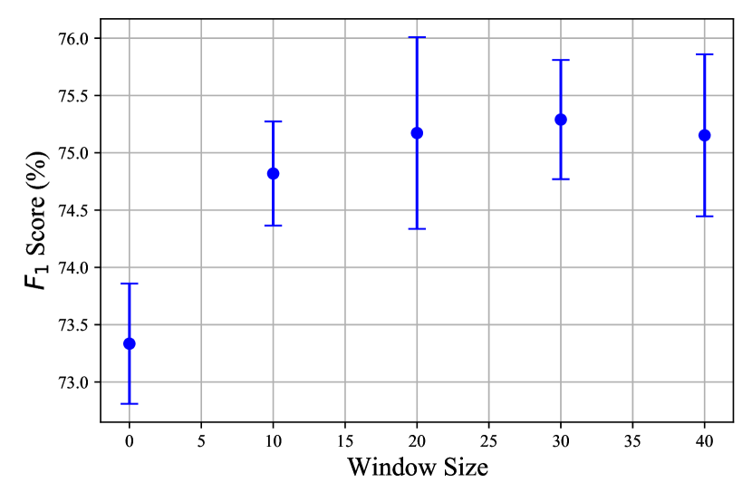
Figure 2: Text GCN performance for varied word co-occurrence window sizes.

As mentioned in section 2, annotated data is particularly difficult to source for Swahili applications. Therefore, it is important to determine the effectiveness of the top performing models when the proportion of labels in the training set is drastically reduced. To this end, figure 3 compares the macro $F_{1}$ scores obtained by both Text GCN variants, TF-IDF, and the PV-DBOW models for training set proportions of 1%, 5%, 10%, and 20%. We find that both Text GCN models consistently outperform the traditional techniques, most noticeably as the proportion of labels is reduced. The TF-IDF and Counts models in particular see a significant degradation in performance when reducing the label proportion from 5% to 1%, while PV-DBOW consistently lags behind both Text GCN models.

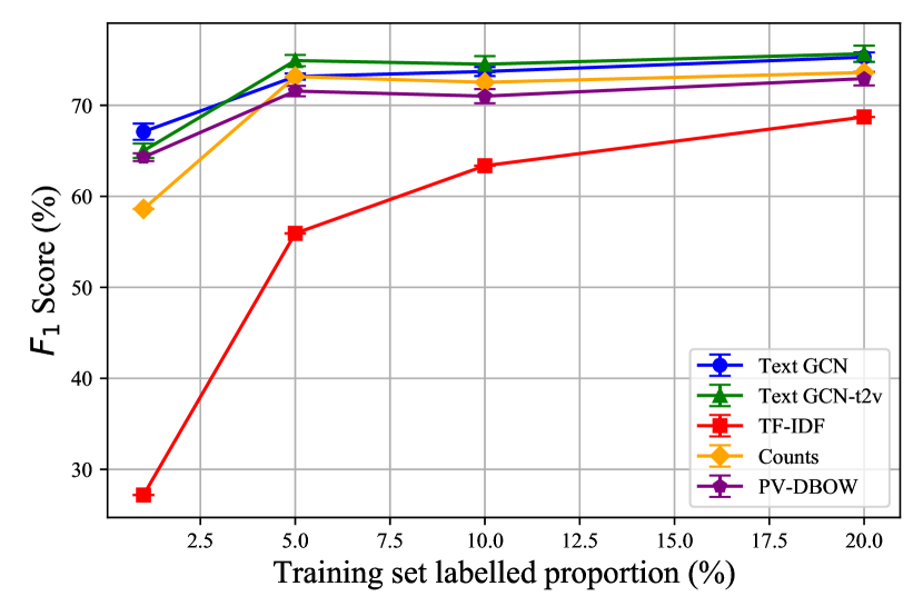
Figure 3: Test set macro $F_{1}$ scores using varying percentages of the training set labels.

5 Conclusion

This paper empirically demonstrates the ability of Text GCN, a model originally developed for English, to outperform traditional models for the task of semi-supervised Swahili news classification. In doing so, we present an accessible set of baselines and demonstrate that when the number of training set labels is reduced, these methods fail to maintain their predictive ability. Finally, our Text GCN-t2v variant imposes a significantly reduced memory cost while continuing to match the predictive performance of the vanilla Text GCN.

Our hope is that these results highlight the applicability of GNNs to semi-supervised Swahili applications more broadly than news categorisation. Future endeavours could extend this work to Swahili speech recognition where decoded outputs are often represented as a directed graph Ragni and Gales (2018); Kastanos et al. (2020).

Appendix A Text GCN Adjacency Matrix

A formal definition of the adjacency matrix, as applied in Text GCN, is provided in equation 2 Yao et al. (2019).

$$A_{ij}=\left\{\begin{array}[]{ll}\textnormal{PMI}(i,j)&i,j\textnormal{ are words; }\textnormal{PMI}(i,j)>0\\ \textnormal{TF-IDF}_{ij}&i\textnormal{ is a document, }j\textnormal{ is a word}\\ 1&i=j\\ 0&\textnormal{else}\end{array}\right.$$ (2)

Through the constraint defined in the first condition, we implicitly interpret word co-occurrence as a Positive Point-wise Mutual Information (PPMI).

$$\textnormal{PPMI}(i,j)=\textnormal{max}\left(\textnormal{PMI}(i,j),\ 0\right)$$ (3)

Using $W(i)$ to indicate the number of sliding windows in which word $i$ occurs and $\#W$ as the total number of sliding windows, we can formulate PMI as follows:

$$\textnormal{PMI}(i,j)=log\left(\frac{p(i,j)}{p(i)p(j)}\right)$$ (4)

where the joint and marginal probabilities are given by equations 5 and 6 respectively.

$$p(i,j)=\frac{W(i,j)}{\textnormal{\#W}}$$ (5)

$$p(i)=\frac{W(i)}{\textnormal{\#W}}$$ (6)

It is worth noting that while applying the renormalisation trick mentioned in section 3.1, we replace the original definition of $\widetilde{A}$ where $\widetilde{A}=A+\mathbb{1}_{N}$, with $\widetilde{A}=A$. This is because the identity diagonal is handled in equation 2.

Appendix B Data Processing

This section describes the preprocessing pipeline applied to the Swahili News Dataset before training any of the baseline models or constructing the graph for the Text GCN models.

First, we drop one of the samples from the initial dataset as it simply contains the string ‘[.]’. A cleaning stage is applied to all remaining samples wherein all text is converted to lower case, Unicode characters are mapped to an ASCII equivalent, some Twitter meta information is removed, and superfluous whitespace characters are stripped.

Next, we tokenize the text into words using word_tokenize from the NLTK library Bird (2006), and exclude stop words, single character words, and words containing non-alphabetical characters. All words which occur more than once are stemmed using the SALAMA language manager Hurskainen (1999, 2004) and words longer than 30 characters are discarded. Finally, we use regular expressions to detect and merge onomatopoeic and laughter tokens to the special tokens onomatopoeia and laughter respectively.

Appendix C Cloud Compute Comparison

This Appendix provides further details on the training comparison between the vanilla Text GCN, which uses one-hot encoding to represent nodes, and the Text GCN-t2v variant, which uses word2vec and doc2vec embeddings to represent the word and document nodes respectively (hence text2vec).

Table 3 compares two cloud machines from Amazon Web Services (AWS). Both machines are CPU only and are billed according to the total time the instance is running. The Text GCN model, with input features $X\in\mathcal{R}^{N\times N}$ requires over $32\ \textnormal{GB}$ of RAM during training, and therefore is trained on the r5a.2xlarge machine. On the other hand, the Text GCN-t2v has a radically reduced input feature space $X\in\mathcal{R}^{N\times 300}$, and therefore requires less than $16\ \textnormal{GB}$ of RAM. This allows us to train it on the significantly cheaper r5a.large machine.

Machine Name	RAM (GB)	$ / Hour
r5a.large	16	0.133
r5a.2xlarge	64	0.532

Table 3: AWS machine and price comparison. Information as of February 2021.

Table 4 presents the billable cloud time required for each model to construct their respective graphs and train to 100 epochs on their respective instances. We note that although the more sophisticated node representation results in Text GCN-t2v taking 15 minutes longer to construct the graph representation, the resulting model trains far quicker that the Text GCN equivalent. As a result, Text GCN-t2v only incurs costs for just over an hour while Text GCN remains running for over 5 hours.

	Text GCN	Text GCN-t2v
Build graph	30	45
Train model	273	16
Total	303	61

Table 4: Cloud time comparison between Text GCN and Text GCN-t2v. All times are reported in minutes.

Combining the information from tables 3 and 4, the total cost to train Text GCN is $\$2.69$ while the cost to train Text GCN-t2v is estimated at $\$0.14$ . This comparative cost analysis motives the reduction factor reported in section 4.4.

References

- Artetxe et al. (2020) Mikel Artetxe, Sebastian Ruder, and Dani Yogatama. 2020. On the cross-lingual transferability of monolingual representations. In Proceedings of the 58th Annual Meeting of the Association for Computational Linguistics, pages 4623–4637, Online. Association for Computational Linguistics.
- Battaglia et al. (2018) Peter W. Battaglia, Jessica B. Hamrick, Victor Bapst, Alvaro Sanchez-Gonzalez, Vinícius Flores Zambaldi, Mateusz Malinowski, Andrea Tacchetti, David Raposo, Adam Santoro, Ryan Faulkner, Çaglar Gülçehre, H. Francis Song, Andrew J. Ballard, Justin Gilmer, George E. Dahl, Ashish Vaswani, Kelsey R. Allen, Charles Nash, Victoria Langston, Chris Dyer, Nicolas Heess, Daan Wierstra, Pushmeet Kohli, Matthew Botvinick, Oriol Vinyals, Yujia Li, and Razvan Pascanu. 2018. Relational inductive biases, deep learning, and graph networks. CoRR, abs/1806.01261.
- Beck et al. (2018) Daniel Beck, Gholamreza Haffari, and Trevor Cohn. 2018. Graph-to-sequence learning using gated graph neural networks. In Proceedings of the 56th Annual Meeting of the Association for Computational Linguistics (Volume 1: Long Papers), pages 273–283, Melbourne, Australia. Association for Computational Linguistics.
- Beltagy et al. (2020) Iz Beltagy, Matthew E. Peters, and Arman Cohan. 2020. Longformer: The long-document transformer.
- Bird (2006) Steven Bird. 2006. NLTK: The Natural Language Toolkit. In Proceedings of the COLING/ACL 2006 Interactive Presentation Sessions, pages 69–72, Sydney, Australia. Association for Computational Linguistics.
- Bodapati et al. (2019) Sravan Bodapati, Spandana Gella, Kasturi Bhattacharjee, and Yaser Al-Onaizan. 2019. Neural word decomposition models for abusive language detection. In Proceedings of the Third Workshop on Abusive Language Online, pages 135–145, Florence, Italy. Association for Computational Linguistics.
- Bojanowski et al. (2017) Piotr Bojanowski, Edouard Grave, Armand Joulin, and Tomas Mikolov. 2017. Enriching word vectors with subword information. Transactions of the Association for Computational Linguistics, 5:135–146.
- Cetoli et al. (2017) Alberto Cetoli, Stefano Bragaglia, Andrew O’Harney, and Marc Sloan. 2017. Graph convolutional networks for named entity recognition. In Proceedings of the 16th International Workshop on Treebanks and Linguistic Theories, pages 37–45, Prague, Czech Republic.
- Conneau et al. (2020) Alexis Conneau, Kartikay Khandelwal, Naman Goyal, Vishrav Chaudhary, Guillaume Wenzek, Francisco Guzmán, Edouard Grave, Myle Ott, Luke Zettlemoyer, and Veselin Stoyanov. 2020. Unsupervised cross-lingual representation learning at scale. In Proceedings of the 58th Annual Meeting of the Association for Computational Linguistics, pages 8440–8451, Online. Association for Computational Linguistics.
- David (2020) Davis David. 2020. Swahili : News classification dataset.
- Eberhard et al. (2020) David M. Eberhard, Gary F. Simons, and Charles D.Fennig. Ethnologue: Languages of the world [online]. 2020.
- Fey et al. (2018) Matthias Fey, Jan Eric Lenssen, Frank Weichert, and Heinrich Müller. 2018. Splinecnn: Fast geometric deep learning with continuous b-spline kernels. In Proceedings of the IEEE Conference on Computer Vision and Pattern Recognition (CVPR).
- Gori et al. (2005) Marco Gori, Gabriele Monfardini, and Franco Scarselli. 2005. A new model for learning in graph domains. In Proceedings. 2005 IEEE International Joint Conference on Neural Networks, 2005., volume 2, pages 729–734 vol. 2.
- Hu et al. (2020) Junjie Hu, Sebastian Ruder, Aditya Siddhant, Graham Neubig, Orhan Firat, and Melvin Johnson. 2020. Xtreme: A massively multilingual multi-task benchmark for evaluating cross-lingual generalization.
- Huang et al. (2019) Lianzhe Huang, Dehong Ma, Sujian Li, Xiaodong Zhang, and Houfeng Wang. 2019. Text level graph neural network for text classification. In Proceedings of the 2019 Conference on Empirical Methods in Natural Language Processing and the 9th International Joint Conference on Natural Language Processing (EMNLP-IJCNLP), pages 3444–3450, Hong Kong, China. Association for Computational Linguistics.
- Hurskainen (2004) Arvi Hurskainen. 2004. Swahili language manager: A storehouse for developing multiple computational applications. Nordic Journal of African Studies, 13(3):363 – 397.
- Hurskainen and Department of World Cultures, University of Helsinki (2016) Arvi Hurskainen and Department of World Cultures, University of Helsinki. 2016. Helsinki Corpus of Swahili 2.0 Annotated Version.
- Hurskainen (1999) Avri Hurskainen. 1999. Salama: Swahili language manager. Nordic Journal of African Studies, 8:139–157.
- Jiang et al. (2020) Zhengbao Jiang, Antonios Anastasopoulos, Jun Araki, Haibo Ding, and Graham Neubig. 2020. X-FACTR: Multilingual factual knowledge retrieval from pretrained language models. In Proceedings of the 2020 Conference on Empirical Methods in Natural Language Processing (EMNLP), pages 5943–5959, Online. Association for Computational Linguistics.
- Jo and Cinarel (2019) Hwiyeol Jo and Ceyda Cinarel. 2019. Delta-training: Simple semi-supervised text classification using pretrained word embeddings. In Proceedings of the 2019 Conference on Empirical Methods in Natural Language Processing and the 9th International Joint Conference on Natural Language Processing (EMNLP-IJCNLP), pages 3458–3463, Hong Kong, China. Association for Computational Linguistics.
- Joshi et al. (2020) Pratik Joshi, Sebastin Santy, Amar Budhiraja, Kalika Bali, and Monojit Choudhury. 2020. The state and fate of linguistic diversity and inclusion in the NLP world. In Proceedings of the 58th Annual Meeting of the Association for Computational Linguistics, pages 6282–6293, Online. Association for Computational Linguistics.
- Kastanos et al. (2020) Alexandros Kastanos, Anton Ragni, and Mark J. F. Gales. 2020. Confidence estimation for black box automatic speech recognition systems using lattice recurrent neural networks. In ICASSP 2020 - 2020 IEEE International Conference on Acoustics, Speech and Signal Processing (ICASSP), pages 6329–6333.
- Kingma and Ba (2015) Diederik P. Kingma and Jimmy Ba. 2015. Adam: A method for stochastic optimization. In 3rd International Conference on Learning Representations, ICLR 2015, San Diego, CA, USA, May 7-9, 2015, Conference Track Proceedings.
- Kipf and Welling (2017) Thomas N. Kipf and Max Welling. 2017. Semi-supervised classification with graph convolutional networks. In 5th International Conference on Learning Representations, ICLR 2017, Toulon, France, April 24-26, 2017, Conference Track Proceedings. OpenReview.net.
- Lample and Conneau (2019) Guillaume Lample and Alexis Conneau. 2019. Cross-lingual language model pretraining. Advances in Neural Information Processing Systems (NeurIPS).
- Le and Mikolov (2014) Quoc Le and Tomas Mikolov. 2014. Distributed representations of sentences and documents. In Proceedings of the 31st International Conference on Machine Learning, volume 32 of Proceedings of Machine Learning Research, pages 1188–1196, Bejing, China. PMLR.
- Marcheggiani and Titov (2017) Diego Marcheggiani and Ivan Titov. 2017. Encoding sentences with graph convolutional networks for semantic role labeling. In Proceedings of the 2017 Conference on Empirical Methods in Natural Language Processing, pages 1506–1515, Copenhagen, Denmark. Association for Computational Linguistics.
- Mihalcea and Tarau (2004) Rada Mihalcea and Paul Tarau. 2004. TextRank: Bringing order into text. In Proceedings of the 2004 Conference on Empirical Methods in Natural Language Processing, pages 404–411, Barcelona, Spain. Association for Computational Linguistics.
- Minaee et al. (2020) Shervin Minaee, Nal Kalchbrenner, Erik Cambria, Narjes Nikzad, Meysam Chenaghlu, and Jianfeng Gao. 2020. Deep Learning Based Text Classification: A Comprehensive Review. arXiv e-prints, page arXiv:2004.03705.
- Ndubuisi-Obi et al. (2019) Innocent Ndubuisi-Obi, Sayan Ghosh, and David Jurgens. 2019. Wetin dey with these comments? modeling sociolinguistic factors affecting code-switching behavior in nigerian online discussions. In Proceedings of the 57th Annual Meeting of the Association for Computational Linguistics, pages 6204–6214, Florence, Italy. Association for Computational Linguistics.
- Niyongabo et al. (2020) Rubungo Andre Niyongabo, Qu Hong, Julia Kreutzer, and Li Huang. 2020. KINNEWS and KIRNEWS: Benchmarking cross-lingual text classification for Kinyarwanda and Kirundi. In Proceedings of the 28th International Conference on Computational Linguistics, pages 5507–5521, Barcelona, Spain (Online). International Committee on Computational Linguistics.
- Orife et al. (2020) Iroro Orife, Julia Kreutzer, Blessing Sibanda, Daniel Whitenack, Kathleen Siminyu, Laura Martinus, Jamiil Toure Ali, Jade Z. Abbott, Vukosi N. Marivate, Salomon Kabongo, Musie Meressa, Espoir Murhabazi, Orevaoghene Ahia, Elan Van Biljon, Arshath Ramkilowan, Adewale Akinfaderin, Alp Öktem, Wole Akin, Ghollah Kioko, Kevin Degila, Herman Kamper, Bonaventure Dossou, Chris Emezue, Kelechi Ogueji, and Abdallah Bashir. 2020. Masakhane - machine translation for africa. CoRR, abs/2003.11529.
- Piergallini et al. (2016) Mario Piergallini, Rouzbeh Shirvani, Gauri S. Gautam, and Mohamed Chouikha. 2016. Word-level language identification and predicting codeswitching points in Swahili-English language data. In Proceedings of the Second Workshop on Computational Approaches to Code Switching, pages 21–29, Austin, Texas. Association for Computational Linguistics.
- Ragni and Gales (2018) Anton Ragni and Mark J.F. Gales. 2018. Automatic speech recognition system development in the ”wild”. In Proceedings of INTERSPEECH, pages 2217–2221.
- Scarselli et al. (2009) Franco Scarselli, Marco Gori, Ah C. Tsoi, Markus Hagenbuchner, and Gabriele Monfardini. 2009. The graph neural network model. IEEE Transactions on Neural Networks, 20(1):61–80.
- Shikali and Mokhosi (2020) Casper S. Shikali and Refuoe Mokhosi. 2020. Enhancing african low-resource languages: Swahili data for language modelling. Data in Brief, 31:105951.
- Strubell et al. (2019) Emma Strubell, Ananya Ganesh, and Andrew McCallum. 2019. Energy and policy considerations for deep learning in NLP. In Proceedings of the 57th Annual Meeting of the Association for Computational Linguistics, pages 3645–3650, Florence, Italy. Association for Computational Linguistics.
- Sun et al. (2020) Chi Sun, Xipeng Qiu, Yige Xu, and Xuanjing Huang. 2020. How to fine-tune bert for text classification?
- Tran (2020) Ke Tran. 2020. From english to foreign languages: Transferring pre-trained language models.
- Veličković et al. (2018) Petar Veličković, Guillem Cucurull, Arantxa Casanova, Adriana Romero, Pietro Liò, and Yoshua Bengio. 2018. Graph attention networks. In International Conference on Learning Representations.
- Wang and Manning (2012) Sida Wang and Christopher Manning. 2012. Baselines and bigrams: Simple, good sentiment and topic classification. In Proceedings of the 50th Annual Meeting of the Association for Computational Linguistics (Volume 2: Short Papers), pages 90–94, Jeju Island, Korea. Association for Computational Linguistics.
- Wang (2017) William Yang Wang. 2017. “liar, liar pants on fire”: A new benchmark dataset for fake news detection. In Proceedings of the 55th Annual Meeting of the Association for Computational Linguistics (Volume 2: Short Papers), pages 422–426, Vancouver, Canada. Association for Computational Linguistics.
- Wu et al. (2021) Z. Wu, S. Pan, F. Chen, G. Long, C. Zhang, and P. S. Yu. 2021. A comprehensive survey on graph neural networks. IEEE Transactions on Neural Networks and Learning Systems, 32(1):4–24.
- Yang et al. (2019) Zhilin Yang, Zihang Dai, Yiming Yang, Jaime Carbonell, Russ R Salakhutdinov, and Quoc V Le. 2019. Xlnet: Generalized autoregressive pretraining for language understanding. In Advances in Neural Information Processing Systems, volume 32, pages 5753–5763. Curran Associates, Inc.
- Yao et al. (2019) Liang Yao, Chengsheng Mao, and Yuan Luo. 2019. Graph convolutional networks for text classification. In AAAI, pages 7370–7377.
- Zaheer et al. (2021) Manzil Zaheer, Guru Guruganesh, Avinava Dubey, Joshua Ainslie, Chris Alberti, Santiago Ontanon, Philip Pham, Anirudh Ravula, Qifan Wang, Li Yang, and Amr Ahmed. 2021. Big bird: Transformers for longer sequences.
- Zhou et al. (2018) Jie Zhou, Ganqu Cui, Zhengyan Zhang, Cheng Yang, Zhiyuan Liu, Lifeng Wang, Changcheng Li, and Maosong Sun. 2018. Graph neural networks: A review of methods and applications. arXiv preprint arXiv:1812.08434.