Intelligent Reflecting Surface-aided URLLC in a Factory Automation Scenario

Abstract

Different from conventional wired line connections, industrial control through wireless transmission is widely regarded as a promising solution due to its reduced cost, increased long-term reliability, and enhanced reliability. However, mission-critical applications impose stringent quality of service (QoS) requirements that entail ultra-reliability low-latency communications (URLLC). The primary feature of URLLC is that the blocklength of channel codes is short, and the conventional Shannon’s Capacity is not applicable. In this paper, we consider the URLLC in a factory automation (FA) scenario. Due to densely deployed equipment in FA, wireless signal are easily blocked by the obstacles. To address this issue, we propose to deploy intelligent reflecting surface (IRS) to create an alternative transmission link, which can enhance the transmission reliability. In this paper, we focus on the performance analysis for IRS-aided URLLC-enabled communications in a FA scenario. Both the average data rate (ADR) and the average decoding error probability (ADEP) are derived under finite channel blocklength for seven cases: 1) Rayleigh fading channel; 2) With direct channel link; 3) Nakagami-m fading channel; 4) Imperfect phase alignment; 5) Multiple-IRS case; 6) Rician fading channel; 7) Correlated channels. Extensive numerical results are provided to verify the accuracy of our derived results.

I Introduction

Nowadays, industry world is evolving into another new paradigm, that is the so-called fourth industrial revolution or Industrial 4.0 [1], in which more advanced manufacturing functions can be realized with the aid of industrial internet-of-things (IIoT). Conventionally, industrial control systems mainly rely on wired network infrastructure, where the central control unit is connected to various machines through wired lines such as copper lines or optical fibers. However, there are some drawbacks by deploying wired lines such as high installation and maintenance costs, limited motion ranges, and vulnerability to wear and tear in the applications with motion actions.

As a result, the adoption of wireless networks is a promising solution to bypass all the aforementioned issues associated with wired lines. However, the industrial communications are totally different from conventional wireless communications. Instead, they require deterministic communications with the stringent quality of service requirements such as ultra reliability and low latency communications by exchanging a small amount of data such as control command data or measurement data. For typical industrial scenarios such as factory automation (FA), the maximum transmission latency is required to be kept within one millisecond, and the packet error probability should range from $10^{-6}$-$10^{-9}$ [2]. In addition, due to the densely deployed equipment such as metal machinery, random movement of objects (robots and trucks), and thick pillars, the wireless signals are more vulnerable to blockages, which can degrade the reliability performance.

To overcome the above hurdle, intelligent reflecting surface (IRS) is regarded as a promising solution, which has attracted considerable research interest from both academia and industry [3, 4, 5]. In particular, IRS is a square or circular panel that consists of a large number of passive reflecting elements, each of which can induce an independent phase shift on the impinging electromagnetic (EM) waves. Hence, by carefully designing the phase shifts of all reflecting elements, the reflected EM waves can be constructively added with the direct signal from the base station (BS) to enhance the signal power at the desired user, which can enhance the system signal-to-noise (SNR) performance.

Most of the existing contributions on IRS focus on the transmission design for various IRS-aided wireless networks by jointly optimizing the active beamforming at the BS and the phase shift matrix at the IRS for perfect channel state information (CSI) in [6, 7, 8, 9, 10, 11, 12, 13, 14, 15], imperfect CSI in [16, 17, 18, 19], or statistical CSI in [20, 21, 22, 23]. Although extensive research efforts have been devoted to the transmission design for IRS-aided networks, only a few works studied the analytical performance in IRS-aided wireless systems [24, 25, 26, 4, 27, 28, 29, 30, 31, 32, 33, 34, 35, 36]. The performance comparison between IRS-aided systems and relaying systems was performed in [24, 25, 26]. For the IRS-aided single user communication system, the symbol error probability (SEP) was derived for the Rayleigh channel in [4], and the coverage probability was analyzed in [27]. The central limit theorem (CLT) was used in [4] and [27] to derive the probability density function (PDF) of signal-to-noise ratio (SNR). Then the Rayleigh channel model was extended to the more general Rician channel in [28, 29] and Nakagami channel in [30]. The outage probability and spectral efficiency were analyzed in [31] for IRS-aided two-way networks. The exact distribution for signal-to-noise ratio (SNR) was derived in [32] for an IRS-aided millimeter wave (mmWave) communication system, where the fluctuating two-ray distribution was adopted to characterize the small-scale fading in the mmWave band. In practical systems, the phase shifts can only be set with finite discrete values, which induce phase errors. Hence, recent contributions have focused on the study of the impact of the phase errors on the system performance [33, 34, 35, 36]. The authors in [33] demonstrated that transmission under imperfect reflectors is equivalent to a point-to-point communication over a Nakagami fading channel. For the IRS-aided physical layer security networks with phase errors, secrecy outage probability and the average secrecy rate was studied in [34] for a single eavesdropper case and in [35] for the case with multiple eavesdroppers.

All the above-mentioned contributions only focused on the traditional services with long packet, in which Shannon’s Capacity is an accurate approximation of the achievable data rate. However, in a factory automation scenario with URLLC requirements, only small packets are transmitted due to the delay limit. In this case, the channel blocklength is finite, and the decoding error probability cannot approach zero for arbitrarily high SNR. Then, Shannon’s Capacity can no longer be applied [37] since the law of large numbers does not hold and it cannot characterize the maximal achievable data rate with given decoding error probability. In fact, simulation results in [38] demonstrated that the delay outage probability will be underestimated if directly using Shannon’s Capacity, and thus the quality of service (QoS) requirements cannot be guaranteed. In the seminal work in [39], by using normal approximation technique the authors have derived the accurate approximation of the maximal achievable rate that is valid under the short blocklength regime for the point-to-point AWGN channel, which is a complicated function of SNR, channel blocklength, and decoding error probability. Most recently, based on the results in [39], extensive research attention has been devoted to the short packet transmission design [40, 41, 42, 43, 44, 45, 46, 47] or performance analysis under the short blocklength regime [48, 49, 50, 51]. However, all these contributions in [40, 41, 42, 52, 43, 44, 45, 46, 47, 48, 49, 50, 51] did not consider the IRS-aided wireless systems. To the best of our knowledge, only a few works have studied the IRS-aided URLLC networks [53, 54]. In [53], the authors proposed a novel polytope-based method to solve the overall decoding error probability minimization problem for an IRS-aided URLLC-enabled UAV system by jointly optimizing the passive beamforming, UAV location and channel blocklength. In [54], the authors studied the resource allocation problem for IRS-aided multiple-input single-output (MISO) orthogonal frequency division multiple access (OFDMA) multicell networks. However, these two papers focused on the transmission design, the analytical performance of IRS-aided systems is not yet available in the existing literature.

Against the above background, we present a comprehensive performance analysis of the end-to-end IRS-aided URLLC-enabled system in a factory automation scenario. Specifically, the main contributions are summarized as follows:

1. We first construct the system model for IRS-aided URLLC in a factory automation scenario. In specific, there is one central control that attempts to send control signals to a remote device. Due to the dense blockage between the transmitter and receiver, the direct signal power is weak. To enhance the communication quality, an IRS is deployed between the transmitter and the receiver, and an alternative transmission link is created to aid the communications. Due to the stringent latency requirement and the small packet size of control signals, the short packet transmission theory should be adopted, which is more complex than conventional Shannon capacity expression.

2. We have derived the closed-form expressions for the average data rate (ADR) and average decoding error probability (ADEP) under finite channel blocklength for seven cases: 1) Rayleigh fading channel; 2) With direct channel link; 3) Nakagami-m fading channel; 4) Imperfect phase alignment; 5) Multiple-IRS case; 6) Rician fading channel; 7) Correlated channels. In specific, the distribution of SNR is first approximated as a Gamma distribution by using the moment matching technique, based on which the ADR is derived in closed form. By using the linearization technique, we also derive the approximate closed-form expression of average decoding error probability (ADEP) under finite channel blocklength.

3. Extensive numerical results obtained from Monte-Carlo simulations demonstrate the accuracy of the derived results and we also provide insightful analysis. Specifically, there is a roughly fixed gap between Shannon capacity and ADR under finite channel blocklength, which implies that the conventional Shannon capacity overestimates the system performance.

The rest of this paper is organized as follows. Section II introduces the system model with IRS-aided point-to-point system along with the short packet theory; Section III is devoted to performance analysis for the simple Rayleigh fading channel. Section IV provides some extensions to six more general cases. Numerical results are presented in Section V to validate the accuracy of the derived results. Finally, the conclusion is drawn in Section VI.

II System Model and Problem Formulation

II-A System Model

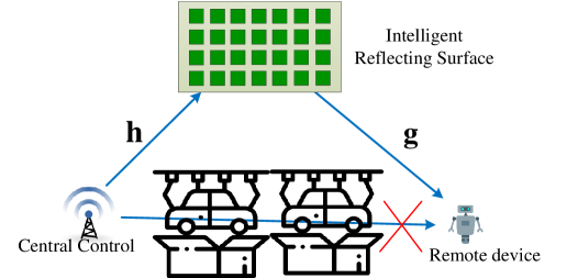
Figure 1: Illustration of an IRS-aided automated factory scenario.

As shown in Fig. 1, we consider an IRS-aided transmission system for an automated factory scenario, where the central controller transmits command signals with short packet size to one remote device (e.g., a robot or an actuator) . Due to the severe blockage caused by huge metallic machines in car manufacturing plants, the channel strength of direct links between the controller and the device is very weak and even lost. The communication link can be established via an IRS installed on the wall or the ceiling of the factory. For the sake of analysis, we assume that the controller and the device are equipped with one single antenna. The IRS is composed of $N$ reflecting phase shifters. The complex channel vectors from the controller to the IRS and from the IRS to the device are denoted by ${\bf{h}}\in\mathbb{C}^{N\times 1}$ and ${\bf{g}}\in\mathbb{C}^{N\times 1}$, respectively. Specifically, the channel vector ${\bf{h}}$ can be represented as ${{\bf{h}}}={\left[{h_{1},\cdots,h_{N}}\right]^{\rm{H}}}$, where $h_{n}$ denotes the complex channel coefficient from the controller to the $n$-th element of the IRS that follows the distribution of ${\cal{CN}}(0,\alpha)$, where ${\cal{CN}}(0,\alpha)$ means the complex Gaussian distribution with zero mean and the variance of $\alpha$. Similarly, we can express ${\bf{g}}$ as ${{\bf{g}}}={\left[{g_{1},\cdots,g_{N}}\right]^{\rm{H}}}$, where $g_{n}$ follows the distribution of ${\cal{CN}}(0,\beta)$. In our analysis, both ${\bf{h}}$ and ${\bf{g}}$ are assumed to be available at the transmitter, which includes the instantaneous realization of ${\bf{h}}$ and ${\bf{g}}$ for the phase shift design at the IRS and the distribution of ${\bf{h}}$ and ${\bf{g}}$ for the performance analysis.

Let us first denote the diagonal reflection-coefficient matrix at the IRS by

$${\bm{\Phi}}={\rm{diag}}\left\{{{e^{j{\phi_{1}}}},\cdots,{e^{j{\phi_{n}}}},\cdots,{e^{j{\phi_{N}}}}}\right\},$$ (1)

where ${\phi_{n}}\in[0,2\pi]$ is the phase shift of the $n$-th element. By assuming that the controller transmits with fixed power $P$, the received signal at the device is given by

$$r=\sqrt{P}{\bf{g}}^{\rm{H}}{\bm{\Phi}}{{\bf{h}}}x+n,$$ (2)

where $x\in\mathbb{C}$ is the data information with unit power, and $n\in\mathbb{C}$ is the noise at the user that follows zero mean and variance of ${\sigma^{2}}$. Then, the instantaneous SNR at the device is given by

$$\gamma=\rho{{{\left|{{\bf{g}}^{\rm{H}}{\bm{\Phi}}{{\bf{h}}}}\right|}^{2}}},$$ (3)

where $\rho=\frac{P}{{{\sigma^{2}}}}$.

II-B Short Packet Transmission Theory

The coding rate for a communication system is defined as the ratio of the number of bits to the total number of channel uses. Shannon capacity is the largest coding rate that can be achieved such that there exists an encoder/decoder pair whose decoding error probability can approach zero when the number of channel uses is sufficiently large [55]. However, for applications in industrial factories, the number of channel uses (channel blocklength) cannot be very large due to the stringent delay requirement. As a result, the decoding error probability will not be equal to zero and has to be reconsidered [46, 47].

Let us first denote the maximum decoding error probability as $\varepsilon$. Then, the maximum instantaneous achievable data rate $R$ (bit/s/Hz) [39] of the remote device can be approximated by

$$R={\log_{2}}\left({1+\gamma}\right)-\sqrt{\frac{V(\gamma)}{M}}\frac{{{Q^{-1}}\left(\varepsilon\right)}}{{\ln 2}},$$ (4)

where $M$ is the number of channel uses, $Q^{-1}(\cdot)$ is the inverse function of $Q(x)\!=\!\frac{1}{{\sqrt{2\pi}}}\int_{x}^{\infty}{{e^{-\frac{{{t^{2}}}}{2}}}dt}$, and $V(\gamma)$ is the channel dispersion given by $V(\gamma)\!=\!1-{(1+\gamma)^{-2}}$. Assume that we require to transmit a packet with $D$ bits within $M$ channel uses. Then, the achievable date rate can be calculated by $R=D/M$, and the corresponding minimum decoding error probability is given by

$${\varepsilon}=Q\left({f\left({{{\gamma}},{M},D}\right)}\right),$$ (5)

where $f\!\left({\gamma,M,D}\right)\!=\!\ln 2\sqrt{\frac{M}{V(\gamma)}}\left({{{\log}_{2}}(1+\gamma)\!-\!\frac{D}{M}}\right)$.

III Performance Analysis

Since the CSI is assumed to be available at the BS, the SNR of $\gamma$ in (3) can be rewritten as

$$\gamma=\rho\left|{\sum\limits_{n=1}^{N}{{g_{n}}{h_{n}}{e^{j{\phi_{n}}}}}}\right|^{2}.$$ (6)

With the aid of CSI at the BS, the optimal $\phi_{n}$ that maximizes the instantaneous $\gamma$ is given by

$${\phi_{n}^{\star}}=-\angle{g_{n}}-\angle{h_{n}}.$$ (7)

Then, $\gamma$ is given by

$$\gamma=\rho{\left({\sum\limits_{n=1}^{N}{\left|{{g_{n}}}\right|\left|{{h_{n}}}\right|}}\right)^{2}}.$$ (8)

Let us define $X\buildrel\Delta\over{=}{\left({\sum\nolimits_{n=1}^{N}{\left|{{g_{n}}}\right|\left|{{h_{n}}}\right|}}\right)^{2}}$. In the following lemma, we approximate $X$ as a Gamma distribution.

Lemma 1: Let us denote the first and second moments of the random variable (RV) $X$ by ${u_{X}}=\mathbb{E}\left\{X\right\}$ and $u_{X}^{(2)}=\mathbb{E}\left\{{{X^{2}}}\right\}$, respectively. Then, the distribution of $X$ can be approximated as a Gamma distribution with the same first and second moments, and its shape $\bar{k}$ and scale $\bar{\theta}$ are given by

$$\bar{k}=\frac{{u_{X}^{2}}}{{u_{X}^{(2)}-u_{X}^{2}}},\bar{\theta}=\frac{{u_{X}^{(2)}-u_{X}^{2}}}{{{u_{X}}}},$$ (9)

where $u_{X}$ and $u_{X}^{(2)}$ are given in (A.5) and (A.7), respectively. The PDF and CDF of $X$ are respectively approximated by

$${f_{X}}(x)=\frac{1}{{\Gamma(\bar{k}){{\bar{\theta}}^{\bar{k}}}}}{x^{\bar{k}-1}}{e^{-\frac{x}{{\bar{\theta}}}}},{F_{X}}(x)=\frac{1}{{\Gamma\left({\bar{k}}\right)}}\gamma\left({\bar{k},\frac{x}{{\bar{\theta}}}}\right).$$ (10)

Proof: Please refer to Appendix A.  

Since $\gamma=\rho X$, we have $\mathbb{E}\{\gamma\}=\rho\mathbb{E}\{X\}$ and $\mathbb{E}\{\gamma^{2}\}=\rho^{2}\mathbb{E}\{X^{2}\}$. Then, $\gamma$ can also be approximated as a Gamma distribution with $k=\bar{k}$ and $\theta=\rho\bar{\theta}$. The PDF and CDF of $\gamma$ are respectively approximated by

$${f_{\gamma}}(x)=\frac{1}{{\Gamma(k){\theta^{k}}}}{x^{k-1}}{e^{-\frac{x}{\theta}}},{F_{X}}(x)=\frac{1}{{\Gamma\left(k\right)}}\gamma\left({k,\frac{x}{\theta}}\right).$$ (11)

Based on the above results, we proceed to derive the ADR and ADEP in the following subsections.

III-A Average Data Rate

It is difficult to get the exact expression of the average data rate (ADR). Next, we show the approximate expression of ADR.

Lemma 2: By using $V(\gamma)=1-\frac{1}{(\gamma+1)^{2}}\approx 1$ when $\gamma$ is large, ADR can be approximated as

$${\bar{R}}\approx\frac{\Gamma({k}-1)\,_{2}F_{2}\left(1,1;2,2-{k};\frac{1}{{\theta}}\right)}{{\theta}(\log(2)\Gamma({k}))}-\frac{{{Q^{-1}}\left(\varepsilon\right)}}{\sqrt{M}\log(2)}+\frac{\psi^{(0)}({k})+\log({\theta})}{\log(2)}+$$ (12)

$$\frac{\left(\pi(-1)^{-{k}}\csc(\pi{k})\right)\gamma\left({k},-\frac{1}{{\theta}}\right)}{\log(2)\Gamma({k})},$$

where ${}_{p}F_{q}(a;b;z)$ is the generalized hypergeometric function [56], ${\psi^{(0)}}(n)$ is the polygamma function [57, 58].

Proof: See Appendix B.  

III-B Average Decoding Error Probability

In this subsection, we aim to derive the ADEP by transmitting a packet with fixed size of $D$ within $M$ channel uses. Then, the ADEP is defined as

$$\bar{\varepsilon}=\int_{0}^{\infty}{Q\left({\ln 2\sqrt{\frac{M}{{V(x)}}}\left({{{\log}_{2}}(1+x)-\frac{D}{M}}\right)}\right){f_{\gamma}}\left(x\right)dx},$$ (13)

where $f_{\gamma}(x)$ is given in (11).

Again, by using the linearization technique to approximate the Q-function, we have the following lemma.

Lemma 3: The closed-form expression of $\bar{\varepsilon}$ can be derived as

$$\bar{\varepsilon}\approx\frac{{\theta}^{-{k}}}{2\Gamma({k})}$$ (14)

$$\left((2{\mu}{x_{0}}+1)\left({x_{0}}+\frac{1}{2{\mu}}\right)^{{k}}E_{-{k}}\left(\frac{{x_{0}}+\frac{1}{2{\mu}}}{{\theta}}\right)-(2{\mu}{x_{0}}-1)\left({x_{0}}-\frac{1}{2{\mu}}\right)^{{k}}E_{-{k}}\left(\frac{{x_{0}}-\frac{1}{2{\mu}}}{{\theta}}\right)\right.$$

$$\left.+{\theta}^{{k}}\left((1+2{\mu}{x_{0}})\gamma\left({k},\frac{{x_{0}}+\frac{1}{2{\mu}}}{{\theta}}\right)+(1-2{\mu}{x_{0}})\gamma\left({k},\frac{{x_{0}}-\frac{1}{2{\mu}}}{{\theta}}\right)\right)\right),$$

where $E_{n}(z)=\int_{1}^{\infty}\frac{e^{-zt}}{t^{n}}dt$ gives the exponential integral function [59].

Proof: See Appendix C.  

IV Extensions to More General Cases

In this section, we consider several possible extensions.

IV-A The existence of direct channel link

In this subsection, we consider the case when there is direct channel link between the BS and the remote device, and its channel coefficient is denoted as $h_{0}$, following the distribution of ${\cal{CN}}(0,\eta)$. Then, the instantaneous SNR at the device is given by

$$\gamma=\rho{{{\left|h_{0}+{{\bf{g}}^{\rm{H}}{\bm{\Phi}}{{\bf{h}}}}\right|}^{2}}}=\rho{{{\left|h_{0}+{\sum\limits_{n=1}^{N}{{g_{n}}{h_{n}}{e^{j{\phi_{n}}}}}}\right|}^{2}}},$$ (15)

where $\rho=\frac{P}{{{\sigma^{2}}}}$.

When CSI is available at the BS, the optimal $\phi_{n}$ that maximizes the instantaneous $\gamma$ is given by

$${\phi_{n}^{\star}}=-\angle{g_{n}}-\angle{h_{n}}+\angle{h_{0}}.$$ (16)

Then, $\gamma$ is given as

$$\gamma=\rho{\left(\left|h_{0}\right|+{\sum\limits_{n=1}^{N}{\left|{{g_{n}}}\right|\left|{{h_{n}}}\right|}}\right)^{2}}=\rho Y,$$ (17)

where $Y=\left(\left|h_{0}\right|+{\sum\nolimits_{n=1}^{N}{\left|{{g_{n}}}\right|\left|{{h_{n}}}\right|}}\right)^{2}$.

In the next lemma, we approximate $Y$ as a Gamma distribution.

Lemma 4: The distribution of $Y$ can be approximated as a Gamma distribution, which is characterized by two parameters $\bar{k}_{Y}$ and $\bar{\theta}_{Y}$, i.e.,

$$Y\sim{\rm{Gamma}}\left({{\bar{k}_{Y}},{\bar{\theta}_{Y}}}\right),$$ (18)

in which the parameters $\bar{k}_{Y}$ and $\bar{\theta}_{Y}$ are given by

$$\bar{k}_{Y}=\frac{{u_{Y}^{2}}}{{u_{Y}^{(2)}-u_{Y}^{2}}},\bar{\theta}_{Y}=\frac{{u_{Y}^{(2)}-u_{Y}^{2}}}{{{u_{Y}}}},$$ (19)

where $u_{Y}$ and $u_{Y}^{(2)}$ are given in (D.2) and (D.5), respectively.

Proof: See Appendix D.  

Since $\gamma=\rho X$, $\gamma$ can also be approximated as a Gamma distribution with $k=\bar{k}_{Y}$ and $\theta=\rho\bar{\theta}_{Y}$. The PDF and CDF of $\gamma$ are respectively approximated by

$${f_{\gamma}}(x)=\frac{1}{{\Gamma(k){\theta^{k}}}}{x^{k-1}}{e^{-\frac{x}{\theta}}},{F_{X}}(x)=\frac{1}{{\Gamma\left(k\right)}}\gamma\left({k,\frac{x}{\theta}}\right).$$ (20)

IV-B Nakagami-$m$ fading channel

The channel links from BS to the IRS and from the IRS to the device are assumed to experience the Nakagami-$m$ fading. Specifically, we assume $\left|{{h_{n}}}\right|\sim{\rm{Nakagami}}({m_{1}},\alpha),\forall n$, and $\left|{{g_{n}}}\right|\sim{\rm{Nakagami}}({m_{2}},\beta),\forall n$, where $m_{1}$ and $m_{2}$ are the parameters that measure the severity of fading, $\alpha$ and $\beta$ are the average channel power gains.

By using the phase shift in (7), the SNR $\gamma$ is given by

$$\gamma=\rho{\left({\sum\limits_{n=1}^{N}{\left|{{g_{n}}}\right|\left|{{h_{n}}}\right|}}\right)^{2}}=\rho Z,$$ (21)

where $Z=\left({\sum\nolimits_{n=1}^{N}{\left|{{g_{n}}}\right|\left|{{h_{n}}}\right|}}\right)^{2}$.

Define ${\xi_{n}}=\left|{{g_{n}}}\right|\left|{{h_{n}}}\right|$. In the following lemma, we approximate $Z$ as a Gamma distribution.

Lemma 5: The distribution of $Z$ can be approximated as a Gamma distribution, which is characterized by two parameters $\bar{k}_{Z}$ and $\bar{\theta}_{Z}$, i.e.,

$$Z\sim{\rm{Gamma}}\left({{\bar{k}_{Z}},{\bar{\theta}_{Z}}}\right),$$ (22)

in which the parameters $\bar{k}_{Z}$ and $\bar{\theta}_{Z}$ are given by

$$\bar{k}_{Z}=\frac{{u_{Z}^{2}}}{{u_{Z}^{(2)}-u_{Z}^{2}}},\bar{\theta}_{Z}=\frac{{u_{Z}^{(2)}-u_{Z}^{2}}}{{{u_{Z}}}},$$ (23)

where $u_{Z}$ and $u_{Z}^{(2)}$ are the same as in (A.5) and (A.7) except that the moments of ${\xi_{n}}$ are given by

$$\mathbb{E}\{\xi_{n}^{k}\}=\frac{{\Gamma\left({{m_{1}}+{k\mathord{\left/{\vphantom{k2}}\right.\kern-1.2pt}2}}\right)\Gamma\left({{m_{2}}+{k\mathord{\left/{\vphantom{k2}}\right.\kern-1.2pt}2}}\right)}}{{\Gamma\left({{m_{1}}}\right)\Gamma\left({{m_{2}}}\right)}}{\left({\frac{{{m_{1}}{m_{2}}}}{{\alpha\beta}}}\right)^{-{k\mathord{\left/{\vphantom{k2}}\right.\kern-1.2pt}2}}}.$$

Proof: The proof is similar to Appendix A, which is omitted for simplicity.  

Based on Lemma 5, the SNR $\gamma=\rho Z$ is approximated as the Gamma distribution $\gamma\sim{\rm{Gamma}}\left({{k},\theta}\right)$, where $k=k_{Z}$ and $\theta=\rho{\theta_{Z}}$. The PDF and CDF of $\gamma$ are given by

$${f_{{\gamma}}}(x)\approx\frac{1}{{\Gamma(k){\theta^{k}}}}{x^{k-1}}{e^{-\frac{x}{\theta}}},{F_{{\gamma}}}(x)\approx\frac{1}{{\Gamma\left(k\right)}}\gamma\left({k,\frac{x}{\theta}}\right).$$ (24)

IV-C Imperfect Phase Alignment

In this subsection, we consider the case when the phase shift cannot be perfectly aligned with the channel phases due to the channel estimation error or limited quantization bits of the phase shifts of the IRS. In this case, the SNR $\gamma$ is given by

$$\gamma=\rho{\left|{\sum\limits_{n=1}^{N}{\left|{{g_{n}}}\right|\left|{{h_{n}}}\right|{e^{j{\omega_{n}}}}}}\right|^{2}},$$ (25)

where $\omega_{n}$ is the phase alignment error that follows the uniform distribution, i.e., ${\omega_{n}}\sim U\left({-\Delta,\Delta}\right)$, and $\Delta$ is a constant characterizing the phase error level. When $\Delta=0$, it reduces to the perfect CSI case in Section III.

Define $G\buildrel\Delta\over{=}{\left|{\sum\limits_{n=1}^{N}{\left|{{g_{n}}}\right|\left|{{h_{n}}}\right|{e^{j{\omega_{n}}}}}}\right|^{2}}$. In the following lemma, we approximate $G$ as a Gamma distribution.

Lemma 6: The distribution of $G$ can be approximated as a Gamma distribution, which is characterized by two parameters $\bar{k}_{G}$ and $\bar{\theta}_{G}$, i.e.,

$$G\sim{\rm{Gamma}}\left({{\bar{k}_{G}},{\bar{\theta}_{G}}}\right),$$ (26)

in which the parameters $\bar{k}_{G}$ and $\bar{\theta}_{G}$ are given by

$$\bar{k}_{G}=\frac{{u_{G}^{2}}}{{u_{G}^{(2)}-u_{G}^{2}}},\bar{\theta}_{G}=\frac{{u_{G}^{(2)}-u_{G}^{2}}}{{{u_{G}}}},$$ (27)

where $u_{G}$ and $u_{G}^{(2)}$ are given in (E.1) and (E.2), respectively.

Proof: See Appendix E.  

Based on Lemma 6, the SNR $\gamma=\rho G$ is approximated as the Gamma distribution $\gamma\sim{\rm{Gamma}}\left({{k},\theta}\right)$, where $k=\bar{k}_{G}$ and $\theta=\rho{\bar{\theta}_{G}}$. The PDF and CDF of $\gamma$ are given by

$${f_{{\gamma}}}(x)\approx\frac{1}{{\Gamma(k){\theta^{k}}}}{x^{k-1}}{e^{-\frac{x}{\theta}}},{F_{{\gamma}}}(x)\approx\frac{1}{{\Gamma\left(k\right)}}\gamma\left({k,\frac{x}{\theta}}\right).$$ (28)

IV-D Multiple-IRS Case

In this subsection, we consider the case when there are multiple IRSs, the number of which is $I$. The IRS are distributed far away such that the channels to/from IRSs are uncorrelated, which can increase the diversity. Denote the channel from the controller to the $i$-th IRS and that from the $i$-th IRS to the user as ${\bf{h}}_{i}$ and ${\bf{g}}_{i}$, respectively. Each element of ${\bf{h}}_{i}$ and ${\bf{g}}_{i}$ follows the distribution of ${\cal{CN}}(0,\alpha_{i})$ and ${\cal{CN}}(0,\beta_{i})$, respectively. Then, the SNR of $\gamma$ can be rewritten as

$$\gamma=\rho{\left|{\sum\limits_{i=1}^{I}{\sum\limits_{n=1}^{N}{{g_{i,n}}{h_{i,n}}{e^{j{\phi_{i,n}}}}}}}\right|^{2}},$$ (29)

where $h_{i,n}$ and $g_{i,n}$ are the $n$-th element of ${\bf{h}}_{i}$ and ${\bf{g}}_{i}$.

With the aid of CSI at the controller, the optimal $\phi_{i,n}$ that maximizes the instantaneous $\gamma$ is given by

$${\phi_{i,n}^{\star}}=-\angle{g_{i,n}}-\angle{h_{i,n}}.$$ (30)

Then, $\gamma$ is given as

$$\gamma=\rho{\left({\sum\limits_{i=1}^{I}{\sum\limits_{n=1}^{N}{\left|{{g_{i,n}}}\right|\left|{{h_{i,n}}}\right|}}}\right)^{2}}.$$ (31)

Define ${\xi_{i,n}}=\left|{{g_{i,n}}}\right|\left|{{h_{i,n}}}\right|$ and $\xi_{i}=\sum\nolimits_{n=1}^{N}{{\xi_{i,n}}}$, then the SNR can be rewritten as $\gamma=\rho{\left({\sum\nolimits_{i=1}^{I}{{\xi_{i}}}}\right)^{2}}=\rho U$, where $U=\left({\sum\nolimits_{i=1}^{I}{{\xi_{i}}}}\right)^{2}$.

In the following lemma, we approximate $U$ as a Gamma distribution.

Lemma 7: The distribution of $U$ can be approximated as a Gamma distribution, which is characterized by two parameters $\bar{k}_{U}$ and $\bar{\theta}_{U}$, i.e.,

$$U\sim{\rm{Gamma}}\left({{\bar{k}_{U}},{\bar{\theta}_{U}}}\right),$$ (32)

in which the parameters $k_{U}$ and $\theta_{U}$ are given by

$$\bar{k}_{U}=\frac{{u_{U}^{2}}}{{u_{U}^{(2)}-u_{U}^{2}}},\bar{\theta}_{U}=\frac{{u_{U}^{(2)}-u_{U}^{2}}}{{{u_{U}}}},$$ (33)

where $u_{U}$ and $u_{U}^{(2)}$ are given in (F.9) and (F.10), respectively.

Proof: See Appendix F.  

Based on Lemma 7, the SNR $\gamma=\rho U$ is approximated as the Gamma distribution $\gamma\sim{\rm{Gamma}}\left({{k},\theta}\right)$, where $k=\bar{k}_{U}$ and $\theta=\rho{\bar{\theta}_{U}}$. The PDF and CDF of $\gamma$ are given by

$${f_{{\gamma}}}(x)\approx\frac{1}{{\Gamma(k){\theta^{k}}}}{x^{k-1}}{e^{-\frac{x}{\theta}}},{F_{{\gamma}}}(x)\approx\frac{1}{{\Gamma\left(k\right)}}\gamma\left({k,\frac{x}{\theta}}\right).$$ (34)

IV-E Rician Fading Channel

In this subsection, we consider the Rician channel model. Specifically, we assume $\left|{{h_{n}}}\right|\sim{\rm{Rician}}(\alpha_{1},\beta_{1}),\forall n$, the PDF of which is given by

$${f_{\left|{{h_{n}}}\right|}}\left(x\right)=\frac{x}{{{\alpha_{1}^{2}}}}\exp\left({-\frac{{{x^{2}}+{\beta_{1}^{2}}}}{{2{\alpha_{1}^{2}}}}}\right){I_{0}}\left({\frac{{x\beta_{1}}}{{{\alpha_{1}^{2}}}}}\right),$$ (35)

where $I_{0}(z)$ is the modified Bessel function of the first kind with order zero. In the above Rician fading, the shape parameter $K=\frac{{\beta_{1}^{2}}}{{2\alpha_{1}^{2}}}$ denotes the ratio of the power contributions by line-of-sight path to the remaining multipaths, and the Scale parameter $\Omega=2\alpha_{1}^{2}+\beta_{1}^{2}$ is the total power received in all paths. In addition, we assume $\left|{{g_{n}}}\right|\sim{\rm{Rician}}(\alpha_{2},\beta_{2}),\forall n$.

By using the phase shift in (7), the SNR $\gamma$ is given by

$$\gamma=\rho{\left({\sum\limits_{n=1}^{N}{\left|{{g_{n}}}\right|\left|{{h_{n}}}\right|}}\right)^{2}}=\rho\left({\sum\limits_{n=1}^{N}{{\xi_{n}}}}\right)^{2}=\rho V,$$ (36)

where we have defined ${\xi_{n}}=\left|{{g_{n}}}\right|\left|{{h_{n}}}\right|$ and $V=\left({\sum\nolimits_{n=1}^{N}{{\xi_{n}}}}\right)^{2}$. Define ${\xi_{n}}=\left|{{g_{n}}}\right|\left|{{h_{n}}}\right|$ and $\xi=\sum\nolimits_{n=1}^{N}{{\xi_{n}}}$. In the following lemma, we approximate $V$ as a Gamma distribution.

Lemma 8: The distribution of $V$ can be approximated as a Gamma distribution, which is characterized by two parameters $\bar{k}_{V}$ and $\bar{\theta}_{V}$, i.e.,

$$V\sim{\rm{Gamma}}\left({{\bar{k}_{V}},{\bar{\theta}_{V}}}\right),$$ (37)

in which the parameters $\bar{k}_{V}$ and $\bar{\theta}_{V}$ are given by

$$\bar{k}_{V}=\frac{{u_{V}^{2}}}{{u_{V}^{(2)}-u_{V}^{2}}},\bar{\theta}_{V}=\frac{{u_{V}^{(2)}-u_{V}^{2}}}{{{u_{V}}}},$$ (38)

where $u_{V}$ and $u_{V}^{(2)}$ are the same as in (A.5) and (A.7) except that the moments of ${\xi_{n}}$ are given by [60]

$$u_{{\xi_{n}}}^{(k)}=\alpha_{1}^{k}{2^{k/2}}\Gamma\left({1+{k\mathord{\left/{\vphantom{k2}}\right.\kern-1.2pt}2}}\right){L_{k/2}}\left({-{{\beta_{1}^{2}}\mathord{\left/{\vphantom{{\beta_{1}^{2}}{2\alpha_{1}^{2}}}}\right.\kern-1.2pt}{2\alpha_{1}^{2}}}}\right),$$

where ${L_{q}}(x)$ denotes a Laguerre polynomial ${L_{q}}(z)={}_{1}{F_{1}}\left({-q;1;z}\right)$.

Proof: The proof is similar to Appendix A, which is omitted for simplicity.  

Then, the random variable $\xi$ follows the Gamma distribution with parameters equal to $Nk_{\xi_{n}}$ and $\theta_{\xi_{n}}$. The following steps are the same as those in Section III.

IV-F Correlated Channels

In this subsection, we consider the correlated channels at the IRS. Specifically, the channels follow the following distribution:

$${\bf{h}}\sim\cal{CN}(\bf{0},\alpha\bf{R_{\rm{ci}}}),{\bf{g}}\sim\cal{CN}(\bf{0},\beta\bf{R_{\rm{id}}}),$$ (39)

where $\bf{R_{\rm{ci}}}$ and $\bf{R_{\rm{id}}}$ are the covariance matrices.

Assume that IRS with $N=N_{\rm{H}}N_{\rm{V}}$ reflecting elements is a two-dimensional rectangular surface, which has $N_{\rm{H}}$ elements per row and $N_{\rm{V}}$ elements per column. Each element is assumed to have size of ${d_{\rm{H}}}\times{d_{\rm{V}}}$, where $d_{\rm{H}}$ and $d_{\rm{V}}$ are the horizontal width and vertical height, respectively. We consider the local spherical coordinate system as in [61], and the location of the $n$th element with respect to the origin is ${{\bf{u}}_{n}}={\left[{0,i(n){d_{\rm{H}}},j(n){d_{\rm{V}}}}\right]^{\rm{T}}}$, where $i(n)={\rm{mod}}(n-1,N_{\rm{H}})$ and $j(n)=\left\lfloor{{{\left({n-1}\right)}\mathord{\left/{\vphantom{{\left({n-1}\right)}{{N_{\rm{H}}}}}}\right.\kern-1.2pt}{{N_{\rm{H}}}}}}\right\rfloor$. Here, ${\rm{mod}}(\cdot,\cdot)$ denotes the modulus operation and $\left\lfloor\cdot\right\rfloor$ is the truncation operation. Then, we have $\bf{R_{\rm{ci}}}=\bf{R_{\rm{id}}}=\bf{R}$, and the element of which is given by

$${\left[{\bf{R}}\right]_{n,m}}={\rm{sinc}}\left({\frac{{2\left\|{{{\bf{u}}_{n}}-{{\bf{u}}_{m}}}\right\|}}{\lambda}}\right),n,m=1,\cdots,N$$ (40)

where ${\rm{sinc}}(x)={{\sin\left({\pi x}\right)}\mathord{\left/{\vphantom{{\sin\left({\pi x}\right)}{\left({\pi x}\right)}}}\right.\kern-1.2pt}{\left({\pi x}\right)}}$ is the sinc function.

Based on the above system model, we then analyze the PDF of the SNR $\gamma=\rho{{{\left|{{\bf{g}}^{\rm{H}}{\bm{\Phi}}{{\bf{h}}}}\right|}^{2}}}$ when only the statistic covariance matrix is available. Here, we fix the value of the phase shift matrix of the IRS at ${\bm{\Phi}}$. In the following lemma, we approximate $\gamma$ as a Gamma distribution.

Lemma 9: The distribution of $\gamma$ can be approximated as a Gamma distribution, which is characterized by two parameters $k_{\gamma}$ and $\theta_{\gamma}$, i.e.,

$$\gamma\sim{\rm{Gamma}}\left({{k_{\gamma}},{\theta_{\gamma}}}\right),$$ (41)

in which the parameters $k_{\gamma}$ and $\theta_{\gamma}$ are given by

$$k_{\gamma}=\frac{{u_{\gamma}^{2}}}{{u_{\gamma}^{(2)}-u_{\gamma}^{2}}},\theta_{\gamma}=\frac{{u_{\gamma}^{(2)}-u_{\gamma}^{2}}}{{{u_{\gamma}}}},$$ (42)

where $u_{\gamma}$ and $u_{\gamma}^{(2)}$ are given in (G.1) and (G.3), respectively.

Proof: See Appendix G.  

V Simulation Results

In this section, numerical results are provided to verify the accuracy of our derived results. For illustration purposes, the simulation parameters are set as follows: $\alpha=\beta=1$ and $M=200$. For the case of ADR, $\varepsilon$ is set to $\varepsilon=10^{-6}$, while for the case of ADEP, the number of bits is set to $D=100$. The other parameters are specified in each simulation figure. The curve labelled as ‘Simulation’ is obtained by averaging over 10000 randomly and uniformly generating channels.

V-A Rayleigh Fading Channel

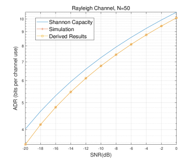
(a) $N=50$

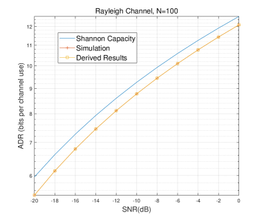
(b) $N=100$

Figure 2: ADR versus SNR $N=50$ and $N=100$ for the case of Rayleigh channel.

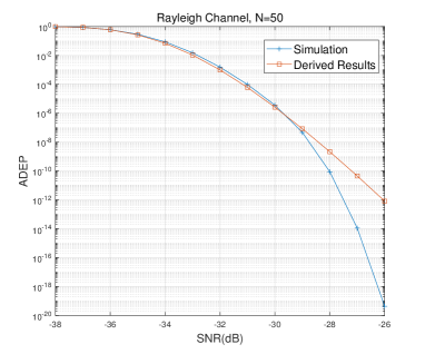
(a) $N=50$

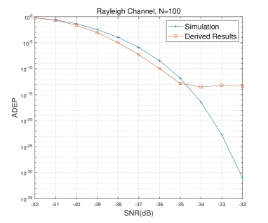
(b) $N=100$

Figure 3: ADEP versus SNR $N=50$ and $N=100$ for the case of Rayleigh channel.

In this subsection, we consider the Rayleigh fading channel.

In Fig. 2, the ADR versus the SNR (in dB) for two different values of $N$. Here, the SNR in the figures is defined as $10{\log_{10}}\rho$, where $\rho=\frac{P}{{{\sigma^{2}}}}$. The curves labelled as ‘Derived Results’ are obtained in (12). For comparison purposes, we also provide the curse based on Shannon’s Capacity that can serve as the performance upper bound. As expected, the ADR increases with SNR, and larger $N$ yields high ADR due to higher passive beamforming gain provided by the IRS. It is also observed from Fig. 2 that the derived results have a perfect agreement with the simulation results for various SNR values and different values of $N$. In addition, there is a constant gap of roughly 0.5 bits per channel use between the Shannon’s capacity and the derived results under the short packet capacity theory.

Fig. 3 depicts the ADEP versus the SNR under two different values of $N$. The curve corresponding to ‘Derived Results’ is obtained by using (14). One can observe from Fig. 3 that when SNR is smaller than -30 dB for the case of $N=50$ and smaller than -35 dB for the case of $N=100$, the derived results coincide with the simulation results, which confirms the accuracy of the derived results and the linearization technique. However, when continuing to increase the SNR value, there is some gap between the derived results and simulation results, and this gap increases with the SNR values. The main reason for this phenomenon is that the value of Q-function will be approximated as zero when the SNR is very large as shown in the third approximation result in (C.1). However, the derived results are very accurate when the ADEP is larger than $10^{-6}$, which generally falls the reliability requirements for most of the URLLC applications.

V-B With Direct Channel Link

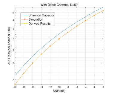
(a) $N=50$

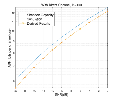
(b) $N=100$

Figure 4: ADR versus SNR for the case with direct channel.

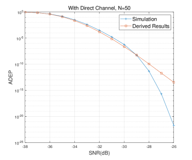
(a) $N=50$

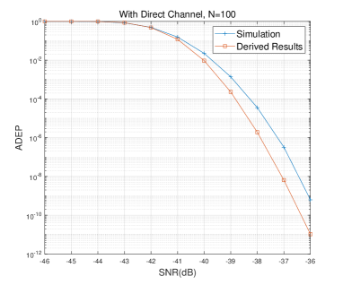
(b) $N=100$

Figure 5: ADEP versus SNR for the case with direct channel.

In this subsection, we consider the case when there is a direct channel link between the BS and the device. The channel gain of the direct channel is assumed to be $\eta=10$.

In Fig. 4, the ADR is shown as a function of SNR for two different values of $N$. The similar trend to Fig. 2 is observed in Fig. 4. In particular, the ADR increases with the values of SNR, and there is a roughly constant gap of 0.5 bit per channel between the Shannon capacity and that of the ADR based on short packet capacity theory. In addition, a larger value of $N$ produces a higher ADR. By comparing Fig. 4-(a) with Fig. 2-(a), the ADR achieved by the case with direct link has a performance gain of 0.2 bit per channel use over the case without direct link when the SNR is equal to -16 dB. However, by comparing the case of $N=50$ with the case of $N=100$ when SNR is equal to -10 dB, we can find 2 bits per channel use can be achieved, which demonstrate the efficiency of using more reflecting elements.

Fig. 5 illustrates the ADEP versus SNR for different values of $N$. From Fig. 5-(a), we can observe that when the SNR is smaller than -30 dB, the derived results are consistent with the simulation results, and can achieve the ADEP as low as $10^{-7}$, which is sufficient for some URLLC applications. However, in the high SNR regime, there is a gap between the derived results and the simulation results, which is mainly due to the approximation error of the linearization technique in the high SNR regime. For Fig. 5-(b), the similar decreasing trend between the ‘Derived results’ and simulation results is observed, and thus the derived results can be used for revealing the diversity order of the ADEP.

V-C Nakagami-$m$ Fading Channel

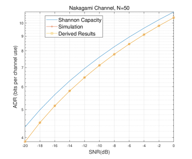
(a) $N=50$

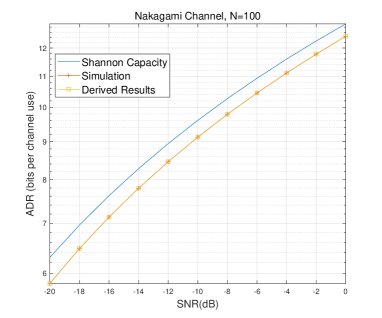
(b) $N=100$

Figure 6: ADR versus SNR for the case of Nakagami channel.

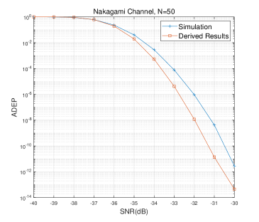
(a) $N=50$

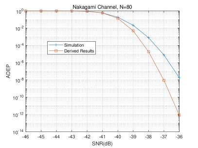
(b) $N=80$

Figure 7: ADEP versus SNR for the case of Nakagami channel.

In this subsection, we consider the case of Nakagami-$m$ fading channel. The parameters of $m_{1}$ and $m_{2}$ that measure the severity of fading are set as $m_{1}=2$ and $m_{2}=2$, respectively.

In Fig. 6, we illustrate the ADR versus the SNR for two different values of $N$. For comparison, the performance of Shannon Capacity is also shown in the figure. It is observed from Fig. 6 that for both values of $N$, the Shannon capacity achieves high ADR than that based on short packet theory, and this gain decreases with the SNR. This shows that the conventional Shannon capacity will overestimate the system performance, and short packet capacity theory should be adopted to measure the system performance for URLLC applications. By comparing Fig. 6-(a) with Fig. 2-(a), we can find that the ADR achieved under the Nakagami-$m$ fading channel is slightly higher than that under the Rayleigh Channel. In addition, the performance gain of 2 bits per channel use can be achieved when increasing $N$ from 50 to 100, which shows the benefits of using more reflecting elements.

In Fig. 7, we illustrate the ADEP versus SNR for different values of $N$. It is again observed that the derived results are accurate when the SNR is very low, and there is approximation error when the SNR is large due to the approximation error of the linearization technique.

V-D Imperfect Phase Alignment

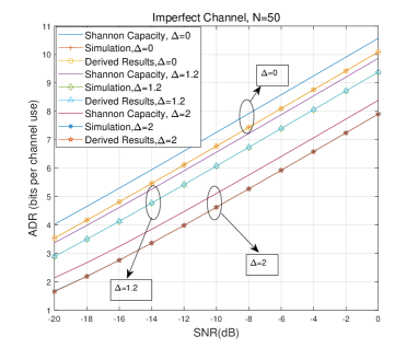
(a) $N=50$

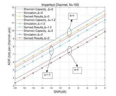
(b) $N=100$

Figure 8: ADR versus SNR for the case of imperfect phase alignment.

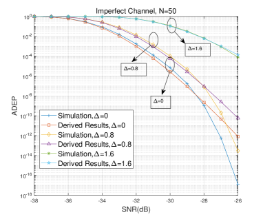
(a) $N=50$

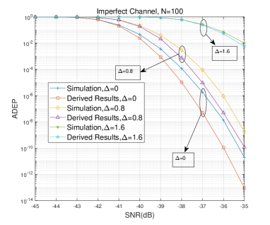
(b) $N=100$

Figure 9: ADEP versus SNR for the case of imperfect phase alignment.

In this subsection, we study the case when there is imperfect phase alignment. The different values of phase alignment error $\Delta$ are shown in the simulation figures.

In Fig. 8, the ADR is shown as a function of SNR for two different values of $N$. Three different values of phase alignment errors are considered: $\Delta=0,1.2,2$. By comparing Fig. 8 for the case of $\Delta=0$ with Fig. 2, we can find that the ADR achieved in both cases is the same, which implies the accuracy of our derived results. As expected, the ADR decreases with the increase of the phase alignment error. In addition, for various values of $\Delta$ and $N$, the derived results are consistent with the simulation results, and verifies the accuracy of the derived results. Larger value of $N$ can achieve larger value of ADR. In addition, higher phase alignment error leads to lower ADR, which means highly precise phase shifts are required to achieve the satisfactory performance.

In Fig. 9, we plot the ADEP versus SNR for two different values of $N$. Three different values of phase alignment errors are considered: $\Delta=0,0.8,1.6$. It is observed from Fig. 9 that the ADEP increases with the increase of the phase alignment error. Specifically, when $N=50$ and SNR is -30 dB, the ADEP increases from $10^{-5}$ to $10^{-1}$. This result demonstrates the importance of obtaining the accurate channel state information. For the case of $N=100$, the ADR achieved by the derived results has almost the same trend as the simulation results although there is some gap between them.

V-E Multiple-IRS Case

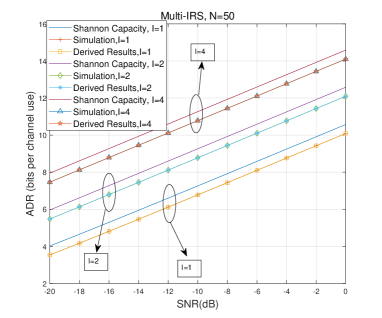
(a) $N=50$

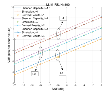
(b) $N=100$

Figure 10: ADR versus SNR for the case of multiple IRSs.

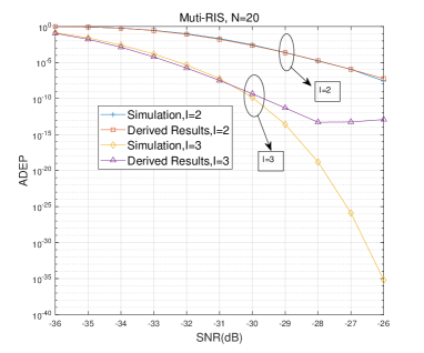
(a) $N=20$

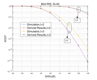
(b) $N=40$

Figure 11: ADEP versus SNR for the case of multiple IRSs.

In this subsection, we consider the case when there are multiple IRSs in the system. The various numbers of IRSs $I$ are shown in the simulation figures.

In Fig. 10, we plot the ADR versus SNR for three different values of $I$ and $N$. It is again observed that the ADR increases with SNR, and larger value of $N$ can achieve higher ADR. As expected, more IRSs can achieve higher ADR due to the increased reflecting beamforming gain. Specifically, by comparing Fig. 10-(a) with Fig. 2-(a), when $I$ increases from 1 to 2 and ${\rm{SNR}}=-12\ \rm{dB}$, the ADR increases from 6 bits per channel use to 8 bits per channel use. Hence, more RISs can increase the ADR performance due to the increased diversity gains.

In Fig. 11, the ADEP versus SNR is plotted for various values of $I$ and $N$. We can observe from Fig. 11 that the ADEP decreases with the increase of $I$ due to the increased beamforming gain. In particular, for the case of $N=20$ and ${\rm{SNR}}=-30\ \rm{dB}$, the ADR decreases from $10^{-3}$ to $10^{-10}$ when increasing $I=2$ to $I=3$, which demonstrates the benefits of using more IRSs. For the case of $N=40$, the derived results have the similar trend as the simulation results although there are some performance differences. This difference is mainly due to the approximation error in the large value of $\gamma$.

V-F Rician Fading Channel

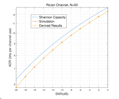
(a) $N=50$

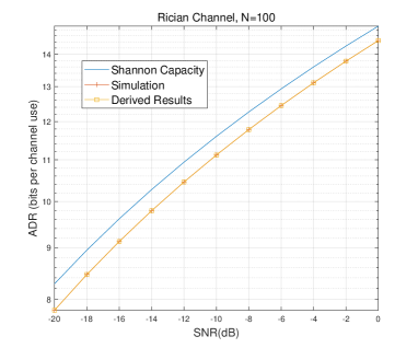
(b) $N=100$

Figure 12: ADR versus SNR for the case of Rician channel.

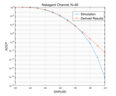
(a) $N=50$

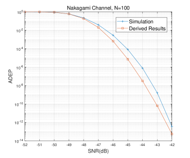
(b) $N=100$

Figure 13: ADEP versus SNR for the case of Rician channel.

In this subsection, we consider the case of Rician channel model, where the parameters are set as $\alpha_{1}=\alpha_{2}=1$, and $\beta_{1}=\beta_{2}=0.5$. Then, the parameter that denotes the ratio of the power contributions by line-of-sight path to the remaining multipaths is $K=1/8$.

In Fig. 12, we illustrate the ADR versus SNR for different values of $N$. Again, it is observed that the simulation results coincide with the derived results, which verifies the accuracy of our derived results. For the case of $N=50$ and ${\rm{SNR}}=-10\ \rm{dB}$, 9 bits per channel use can be achieved for the case of Rician channel, while only 6.8 bits per channel use is achieved for the case of Rayleigh channel model. This shows the advantage of using line-of-sight links in IRS-aided communications. In addition, the benefits of using more reflecting elements are also demonstrated in Fig. 12.

In Fig. 13, the ADEP versus SNR is plotted for two values of $N$. For the case of $N=50$, the derived results are very accurate when ${\rm{SNR}}\leq-37\ \rm{dB}$, and the ADEP can be as low as $10^{-6}$, which are enough for some URLLC applications. It is observed there is performance difference between the derived results and the simulation results when ${\rm{SNR}}\geq-38\ \rm{dB}$, which is due the approximation error due to the large value of $\gamma$. The similar phenomenon is observed for the case of $N=100$.

V-G Correlated Channels

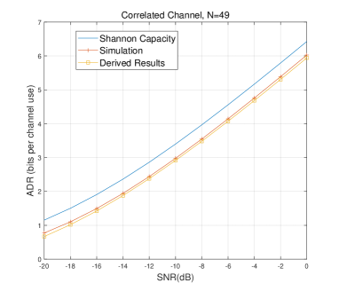
(a) $N=50$

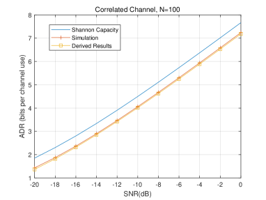
(b) $N=100$

Figure 14: ADR versus SNR for the case of correlated channel.

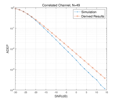
(a) $N=50$

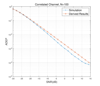
(b) $N=100$

Figure 15: ADEP versus SNR for the case of correlated channel.

Finally, we consider the case when there is correlation among the reflecting elements at the IRS. The parameters are set as follows: $d_{H}=d_{V}=\lambda/4$, and $N_{H}=N_{V}$.

In Fig. 14, we plot the ADR versus the SNR for two different values of $N$. It can be observed from Fig. 14 that the ADR increases with the SNR as expected. However, by comparing Fig. 14 with Fig. 2, we can find that the performance under the correlated channel is much lower than that of the uncorrelated channel. This implies that the correlation significantly affects the ADR performance, and the element spacing should be large to reduce the coupling and correlation among the elements.

In Fig. 15, the ADEP is shown as a function of SNR. It is observed that the ADEP decreases with SNR, and the ADEP achieved in the case of correlated channel is significantly lower than that without correlation. This again demonstrates the importance of enlarging the element spacing distance to eliminate the mutual correlation.

VI Conclusions

In this paper, we proposed to deploy an IRS in a FA scenario to support the URLLC. Different from the existing contributions on transmission design, this paper focused on the analytical analysis by characterizing the performance under the assistance of IRS. To this end, the performance analysis is performed for seven cases: 1) Rayleigh fading channel; 2) With direct channel link; 3) Nakagami-m fading channel; 4) Imperfect phase alignment; 5) Multiple-IRS case; 6) Rician fading channel; 7) Correlated channels. The approximate/accurate ADR and ADEP expressions were derived in closed-form. Extensive numerical results were provided to validate the accuracy of our derived results.

In this work, the phase shifts of the IRS are designed based on the instantaneous CSI, which entails high channel estimation overhead. One promising future direction is to design the phase shifts based on statistical CSI such as angle/location information that varies much slower than the instantaneous CSI. Hence, channel estimation overhead can be significantly reduced. In addition, only one transmit antenna is assumed to be equipped at the base station. To serve more devices with the same time and frequency resources, multiple-antenna technique is a promising research direction due to the fact that it can provide enough spatial degrees of freedom. However, the performance analysis for this case is more complicated, and would leave it for future work. Furthermore, in smart factories with limited space, the transmission distance between the IRS and the devices may fall into the near-field regime. In this case, the conventional uniform plane wave (UPW)-based channel model may become inaccurate, and the near-field radiation with spherical wavefront may appear. How to analyze the performance in the near filed would be challenging but practical, and we will leave it to our future work.

Appendix A Proof of Lemma 1

Define ${\xi_{n}}=\left|{{g_{n}}}\right|\left|{{h_{n}}}\right|$. When $|h_{n}|$ and $|g_{n}|$ are Rayleigh distributions, we have

$$\mathbb{E}\left\{{{\xi_{n}}}\right\} = \frac{\pi}{4}\sqrt{\alpha\beta},\forall n$$ (A.1)

$$\mathbb{E}\left\{{\xi_{n}^{2}}\right\} = \mathbb{E}\left\{{{{\left|{{g_{n}}}\right|}^{2}}{{\left|{{h_{n}}}\right|}^{2}}}\right\}=\alpha\beta,\forall n$$ (A.2)

$$\mathbb{E}\left\{{\xi_{n}^{3}}\right\} = \mathbb{E}\left\{{{{\left|{{g_{n}}}\right|}^{3}}{{\left|{{h_{n}}}\right|}^{3}}}\right\}=\frac{9}{{16}}\pi{\left({\alpha\beta}\right)^{\frac{3}{2}}},\forall n$$ (A.3)

$$\mathbb{E}\left\{{\xi_{n}^{4}}\right\} = \mathbb{E}\left\{{{{\left|{{g_{n}}}\right|}^{4}}{{\left|{{h_{n}}}\right|}^{4}}}\right\}=4{\left({\alpha\beta}\right)^{2}},\forall n.$$ (A.4)

Then, $X$ can be rewritten as $X\buildrel\Delta\over{=}{\left({\sum\nolimits_{n=1}^{N}{\xi_{n}}}\right)^{2}}$. The first moment of the RV $X$ can be calculated by

$$u_{X}=\mathbb{E}\left\{X\right\}=\sum\limits_{n=1}^{N}{\mathbb{E}\left\{{\xi_{n}^{2}}\right\}}+\sum\limits_{n=1}^{N}{\sum\limits_{m=1,m\neq n}^{N}{\mathbb{E}\left\{{{\xi_{n}}}\right\}\mathbb{E}\left\{{{\xi_{m}}}\right\}}},$$ (A.5)

which can be calculated by using (A.1) and (A.2).

The second moment of $X$ can be calculated as follows:

$$u_{X}^{(2)} = \mathbb{E}\left\{{{X^{2}}}\right\}=\mathbb{E}\left\{{{{\left({\sum\limits_{n=1}^{N}{{\xi_{n}}}}\right)}^{4}}}\right\}=\mathbb{E}\left\{{{{\left({\sum\limits_{n=1}^{N}{\xi_{n}^{2}}+\sum\limits_{n=1}^{N}{\sum\limits_{m=1,m\neq n}^{N}{{\xi_{n}}}}{\xi_{m}}}\right)}^{2}}}\right\}$$ (A.7)

$$= \sum\limits_{n=1}^{N}{\mathbb{E}\left\{{\xi_{n}^{4}}\right\}}+4\sum\limits_{n=1}^{N}{\sum\limits_{m=1,m\neq n}^{N}{\mathbb{E}\left\{{\xi_{n}^{3}{\xi_{m}}}\right\}}}+3\sum\limits_{n=1}^{N}{\sum\limits_{m=1,m\neq n}^{N}{\mathbb{E}\left\{{\xi_{n}^{2}\xi_{m}^{2}}\right\}}}$$

$$+6\sum\limits_{{n_{1}}=1}^{N}{\sum\limits_{{n_{2}}=1,n_{2}\neq n_{1}}^{N}{\sum\limits_{{n_{3}}=1,n_{3}\neq n_{2},n_{3}\neq n_{1}}^{N}{\mathbb{E}\left\{{\xi_{{n_{1}}}^{2}{\xi_{{n_{2}}}}{\xi_{{n_{3}}}}}\right\}}}}$$

$$+\sum\limits_{{n_{1}}=1}^{N}{\sum\limits_{{n_{2}}\neq{n_{1}}}{\sum\limits_{{n_{3}}\neq{n_{2}},{n_{3}}\neq{n_{1}}}{\sum\limits_{{n_{4}}\neq{n_{1}},{n_{2}},{n_{3}}}{\mathbb{E}\left\{{{\xi_{{n_{1}}}}{\xi_{{n_{2}}}}{\xi_{{n_{3}}}}{\xi_{{n_{4}}}}}\right\}}}}}.$$

By using the independence between $\xi_{n}$ and $\xi_{m}$, and using (A.1)-(A.4), we can calculate the second moment of $X$.

Appendix B Proof of Lemma 2

By using the approximate PDF of $\gamma$ in (11), ${\bar{R}}$ can be approximated as

$${\bar{R}} = \int_{0}^{\infty}{\left({{{\log}_{2}}\left({1+x}\right)-\frac{{{Q^{-1}}\left(\varepsilon\right)}}{{\ln 2}}\sqrt{\frac{{V(x)}}{M}}}\right){f_{\gamma}}\left(x\right)dx}$$ (B.1)

$$= \!\!\!\frac{1}{{{\theta^{k}}\Gamma(k)}}\underbrace{\int_{0}^{\infty}{{\gamma^{k-1}}}{e^{-\frac{\gamma}{\theta}}}{{\log}_{2}}(1+\gamma)d\gamma}_{{U_{1}}}-\frac{{{Q^{-1}}\left(\varepsilon\right)}}{{\log(2){\theta^{k}}\Gamma(k)}}\underbrace{\int_{0}^{\infty}{{\gamma^{k-1}}}\sqrt{\frac{{1-\frac{1}{{{{(\gamma+1)}^{2}}}}}}{M}}{e^{-\frac{\gamma}{\theta}}}d\gamma}_{{U_{2}}}.$$

Then, $U_{1}$ in (B.1) can be further simplified as

$$U_{3} =\frac{\left(-\frac{1}{{\theta}^{2}}\right)^{-{k}}{\theta}^{-{k}-1}}{\log(2)}$$ (B.2)

$$\left(\left(-\frac{1}{{\theta}}\right)^{{k}}{\theta}^{{k}}\left(\Gamma({k}-1)\,_{2}F_{2}\left(1,1;2,2-{k};\frac{1}{{\theta}}\right)+{\theta}\Gamma({k})(\psi^{(0)}({k})+\log({\theta}))\right)\right.$$

$$\left.+\pi{\theta}\csc(\pi{k})\left(\Gamma({k})-\Gamma\left({k},-\frac{1}{{\theta}}\right)\right)\right)$$

$$=\frac{(-1)^{-{k}}{\theta}^{{k}-1}}{\log(2)}\left((-1)^{{k}}\left(\Gamma({k}-1)\,_{2}F_{2}\left(1,1;2,2-{k};\frac{1}{{\theta}}\right)+{\theta}\Gamma({k})(\psi^{(0)}({k})+\log({\theta}))\right)\right.$$

$$\left.+\pi{\theta}\csc(\pi{k})\left(\Gamma({k})-\Gamma\left({k},-\frac{1}{{\theta}}\right)\right)\right)$$

where ${\psi^{(0)}}(n)$ is the logarithmic Gamma function [57, 58].

By using $V(\gamma)=1-\frac{1}{(\gamma+1)^{2}}\approx 1$, $U_{2}$ can be written as

$$U_{4}\approx\sqrt{\frac{1}{M}}{\theta}^{{k}}\Gamma({k})$$ (B.3)

Then, ${\bar{R}}$ in (B.1) can be approximated as

$${\bar{R}}\approx\frac{\Gamma({k}-1)\,_{2}F_{2}\left(1,1;2,2-{k};\frac{1}{{\theta}}\right)}{{\theta}(\log(2)\Gamma({k}))}-\frac{{{Q^{-1}}\left(\varepsilon\right)}}{\sqrt{M}\log(2)}+\frac{\psi^{(0)}({k})+\log({\theta})}{\log(2)}$$ (B.4)

$$+\frac{\left(\pi(-1)^{-{k}}\csc(\pi{k})\right)\left(\Gamma({k})-\Gamma\left({k},-\frac{1}{{\theta}}\right)\right)}{\log(2)\Gamma({k})}$$

which can be further simplified as (12).

Appendix C Proof of Lemma 3

We adopt the linearization technique to approximate ${Q\left({\ln 2\sqrt{\frac{M}{{V(x)}}}\left({{{\log}_{2}}(1+x)-\frac{D}{M}}\right)}\right)}$ at point $x=x_{0}$ as:

$$\begin{array}[]{l}Q\left({\ln 2\sqrt{\frac{M}{{V(x)}}}\left({{{\log}_{2}}(1+x)-\frac{D}{M}}\right)}\right)\\ \approx U(x)=\left\{\begin{array}[]{l}1,x\leq{x_{0}}-\frac{1}{{2\mu}},\\ \frac{1}{2}-\mu\left({x-{x_{0}}}\right),x\in\left[{{x_{0}}-\frac{1}{{2\mu}},{x_{0}}+\frac{1}{{2\mu}}}\right],\\ 0,x\geq{x_{0}}+\frac{1}{{2\mu}},\end{array}\right.\end{array}$$ (C.1)

where $\mu$ is the value of the first-order derivative of Q-function at point $x=x_{0}$, given by

$$\mu=-{\left.{\frac{{\partial\left({Q\left({\ln 2\sqrt{\frac{M}{{V(x)}}}\left({{{\log}_{2}}(1+x)-\frac{D}{M}}\right)}\right)}\right)}}{{\partial x}}}\right|_{x={x_{0}}}}=\sqrt{\frac{M}{{2\pi\left({{2^{\frac{{2D}}{M}}}-1}\right)}}}.$$ (C.2)

In addition, $x_{0}$ is given by ${x_{0}}={2^{\frac{D}{M}}}-1$.

By inserting (C.1) into (13), the ADEP $\bar{\varepsilon}$ can be approximated as

$$\bar{\varepsilon} \approx{F_{\gamma}}\left({{x_{0}}-\frac{1}{{2\mu}}}\right)+\left({\frac{1}{2}+\mu{x_{0}}}\right)\left({{F_{\gamma}}\left({{x_{0}}+\frac{1}{{2\mu}}}\right)-{F_{\gamma}}\left({{x_{0}}-\frac{1}{{2\mu}}}\right)}\right)-\mu\int_{{x_{0}}-\frac{1}{{2\mu}}}^{{x_{0}}+\frac{1}{{2\mu}}}{x{f_{\gamma}}\left(x\right)dx}$$ (C.3)

$$=\frac{{\mu}}{{\theta}^{{k}}\Gamma({k})}\underbrace{\int_{{x_{0}}-\frac{1}{{2\mu}}}^{{x_{0}}+\frac{1}{{2\mu}}}{\gamma}^{{k}}e^{-\frac{{\gamma}}{{\theta}}}dx}_{U_{6}}$$

$$\quad+\left(\mu x_{0}+\frac{1}{2}\right)\left({F_{\gamma}}\left(\frac{1}{2\mu}+x_{0}\right)-{F_{\gamma}}\left(x_{0}-\frac{1}{2\mu}\right)\right)+{F_{\gamma}}\left(x_{0}-\frac{1}{2\mu}\right).$$

Then, $U_{6}$ can be solved as

$$U_{6}=\left({x_{0}}-\frac{1}{2{\mu}}\right)^{{k}+1}E_{-{k}}\left(\frac{{x_{0}}-\frac{1}{2{\mu}}}{{\theta}}\right)-\left(\frac{1}{2{\mu}}+{x_{0}}\right)^{{k}+1}E_{-{k}}\left(\frac{{x_{0}}+\frac{1}{2{\mu}}}{{\theta}}\right)$$ (C.4)

Then, after some transformation, one can have (14).

Appendix D Proof of Lemma 4

Let us define $\xi_{n}\buildrel\Delta\over{=}\left|{{g_{n}}}\right|\left|{{h_{n}}}\right|,n=1,\cdots,N$ and $\xi_{N+1}=\left|h_{0}\right|$. Then, $Y$ can be rewritten as $Y={\left({\sum\nolimits_{n=1}^{N+1}{{\xi_{n}}}}\right)^{2}}$. For $1\leq n\leq N$, the moments of $\xi_{n}$ are given in (A.1)-(A.4). For $n=N+1$, the moments of $\xi_{n}$ are given by

$$\mathbb{E}\left\{{{\xi_{n}}}\right\}=\frac{{\sqrt{\pi\eta}}}{2},\mathbb{E}\left\{{\xi_{n}^{2}}\right\}=\eta,\mathbb{E}\left\{{\xi_{n}^{3}}\right\}=\frac{3}{4}\sqrt{\pi}{\eta^{\frac{3}{2}}},\mathbb{E}\left\{{\xi_{n}^{4}}\right\}=2{\eta^{2}},n=N+1.$$ (D.1)

Then, by using the similar methods in Appendix A, we have

$$u_{Y}=\mathbb{E}\left\{Y\right\}=\sum\limits_{n=1}^{N+1}{\mathbb{E}\left\{{\xi_{n}^{2}}\right\}}+\sum\limits_{n=1}^{N+1}{\sum\limits_{m=1,m\neq n}^{N+1}{\mathbb{E}\left\{{{\xi_{n}}}\right\}\mathbb{E}\left\{{{\xi_{m}}}\right\}}},$$ (D.2)

and

$$u_{Y}^{(2)} = \sum\limits_{n=1}^{N+1}{\mathbb{E}\left\{{\xi_{n}^{4}}\right\}}+4\sum\limits_{n=1}^{N+1}{\sum\limits_{m=1,m\neq n}^{N+1}{\mathbb{E}\left\{{\xi_{n}^{3}{\xi_{m}}}\right\}}}+3\sum\limits_{n=1}^{N+1}{\sum\limits_{m=1,m\neq n}^{N+1}{\mathbb{E}\left\{{\xi_{n}^{2}\xi_{m}^{2}}\right\}}}$$ (D.5)

$$+6\sum\limits_{{n_{1}}=1}^{N+1}{\sum\limits_{{n_{2}}=1,n_{2}\neq n_{1}}^{N+1}{\sum\limits_{{n_{3}}=1,n_{3}\neq n_{2},n_{3}\neq n_{1}}^{N+1}{\mathbb{E}\left\{{\xi_{{n_{1}}}^{2}{\xi_{{n_{2}}}}{\xi_{{n_{3}}}}}\right\}}}}$$

$$+\sum\limits_{{n_{1}}=1}^{N}{\sum\limits_{{n_{2}}\neq{n_{1}}}{\sum\limits_{{n_{3}}\neq{n_{2}},{n_{3}}\neq{n_{1}}}{\sum\limits_{{n_{4}}\neq{n_{1}},{n_{2}},{n_{3}}}{\mathbb{E}\left\{{{\xi_{{n_{1}}}}{\xi_{{n_{2}}}}{\xi_{{n_{3}}}}{\xi_{{n_{4}}}}}\right\}}}}}$$

Appendix E Proof of Lemma 6

Let us define ${\xi_{n}}=\left|{{g_{n}}}\right|\left|{{h_{n}}}\right|$. Then, $G$ can be rewritten as $G\buildrel\Delta\over{=}{\left|{\sum\nolimits_{n=1}^{N}{{\xi_{n}}{e^{j{\omega_{n}}}}}}\right|^{2}}$. The first moment of the RV $G$ can be calculated by

$${u_{G}} = \mathbb{E}\{G\}=\mathbb{E}\left\{{{{\left|{\sum\limits_{n=1}^{N}{{\xi_{n}}{e^{j{\omega_{n}}}}}}\right|}^{2}}}\right\}$$ (E.1)

$$= \mathbb{E}\left\{{\sum\limits_{n=1}^{N}{\xi_{n}^{2}}+\sum\limits_{n=1}^{N}{\sum\limits_{m=1,m\neq n}^{N}{{\xi_{n}}{\xi_{m}}\cos({\omega_{n}}-{\omega_{m}})}}}\right\}$$

$$= \sum\limits_{n=1}^{N}{\mathbb{E}\left\{{\xi_{n}^{2}}\right\}}+\sum\limits_{n=1}^{N}{\sum\limits_{m=1,m\neq n}^{N}{\mathbb{E}\left\{{{\xi_{n}}}\right\}\mathbb{E}\left\{{{\xi_{m}}}\right\}\mathbb{E}\left\{{\cos({\omega_{n}}-{\omega_{m}})}\right\}}}.$$

where $\mathbb{E}\left\{{\xi_{n}^{2}}\right\}$ and $\mathbb{E}\left\{{{\xi_{n}}}\right\}$ can be calculated by using (A.1) and (A.2). By using some simple calculations, we have $\mathbb{E}\left\{{\cos({\omega_{n}}-{\omega_{m}})}\right\}={\left({\frac{{\sin\Delta}}{\Delta}}\right)^{2}},\forall m\neq n$.

The second moment of $G$ can be calculated as follows:

$$u_{G}^{(2)} = \mathbb{E}\left\{{{{\left|{\sum\limits_{n=1}^{N}{{\xi_{n}}{e^{j{\omega_{n}}}}}}\right|}^{4}}}\right\}=\mathbb{E}\left\{{{{\left({\sum\limits_{n=1}^{N}{\xi_{n}^{2}}+\sum\limits_{n=1}^{N}{\sum\limits_{m=1,m\neq n}^{N}{{\xi_{n}}{\xi_{m}}\cos({\omega_{n}}-{\omega_{m}})}}}\right)}^{2}}}\right\}$$ (E.2)

$$= {\sum\limits_{n=1}^{N}{\mathbb{E}\left\{{\xi_{n}^{4}}\right\}}+2\sum\limits_{n=1}^{N}{\sum\limits_{m\neq n}{\mathbb{E}\left\{{\xi_{n}^{2}\xi_{m}^{2}{{\cos}^{2}}\left({{\omega_{n}}-{\omega_{m}}}\right)}\right\}}}}$$

$$+\sum\limits_{n=1}^{N}{\sum\limits_{m\neq n}{\mathbb{E}\left\{{\xi_{n}^{2}\xi_{m}^{2}}\right\}}}+4\sum\limits_{n=1}^{N}{\sum\limits_{m\neq n}{\mathbb{E}\left\{{\xi_{n}^{3}{\xi_{m}}\cos\left({{\omega_{n}}-{\omega_{m}}}\right)}\right\}}}$$

$$+2\sum\limits_{{n_{1}}=1}^{N}{\sum\limits_{{n_{2}}\neq{n_{1}}}{\sum\limits_{{n_{3}}\neq{n_{1}},{n_{2}}}{\mathbb{E}\left\{{\xi_{{n_{1}}}^{2}{\xi_{{n_{2}}}}{\xi_{{n_{3}}}}\cos\left({{\omega_{{n_{2}}}}-{\omega_{{n_{3}}}}}\right)}\right\}}}}$$

$${+4\sum\limits_{{n_{1}}=1}^{N}{\sum\limits_{{n_{2}}\neq{n_{1}}}{\sum\limits_{{n_{3}}\neq{n_{1}},{n_{2}}}{\mathbb{E}\left\{{\xi_{{n_{1}}}^{2}{\xi_{{n_{2}}}}{\xi_{{n_{3}}}}\cos\left({{\omega_{{n_{1}}}}-{\omega_{{n_{2}}}}}\right)\cos\left({{\omega_{{n_{1}}}}-{\omega_{{n_{3}}}}}\right)}\right\}}}}}$$

$${+\sum\limits_{{n_{1}}=1}^{N}{\sum\limits_{{n_{2}}\neq{n_{1}}}{\sum\limits_{{n_{3}}\neq{n_{1}},{n_{2}}}{\sum\limits_{{n_{4}}\neq{n_{1}},{n_{2}},{n_{3}}}{\mathbb{E}\left\{{{\xi_{{n_{1}}}}{\xi_{{n_{2}}}}{\xi_{{n_{3}}}}{\xi_{{n_{4}}}}\cos\left({{\omega_{{n_{1}}}}-{\omega_{{n_{2}}}}}\right)\cos\left({{\omega_{{n_{3}}}}-{\omega_{{n_{4}}}}}\right)}\right\}}}}}}.$$

By using some simple calculations, we have

$$\mathbb{E}\left\{{{{\cos}^{2}}\left({{\omega_{n}}-{\omega_{m}}}\right)}\right\} = \frac{1}{2}+\frac{1}{2}{\left({\frac{{\sin\left({2\Delta}\right)}}{{2\Delta}}}\right)^{2}}$$ (E.3)

$$\mathbb{E}\left\{{\cos\left({{\omega_{{n_{1}}}}-{\omega_{{n_{2}}}}}\right)\cos\left({{\omega_{{n_{1}}}}-{\omega_{{n_{3}}}}}\right)}\right\} = \frac{{\sin(\Delta)\cos\left(\Delta\right)+4\Delta{{\sin}^{2}}(\Delta)-\sin(\Delta)\cos(3\Delta)}}{{8{\Delta^{3}}}}.$$ (E.4)

Then, by using (A.1)-(A.4) and the above equalities, we can calculate the second moment of $G$.

Appendix F Proof of Lemma 7

For each $i$, we have

$$\mathbb{E}\left\{{{\xi_{i,n}}}\right\} = \frac{\pi}{4}\sqrt{\alpha_{i}\beta_{i}},\forall n$$ (F.1)

$$\mathbb{E}\left\{{\xi_{i,n}^{2}}\right\} = \mathbb{E}\left\{{{{\left|{{g_{i,n}}}\right|}^{2}}{{\left|{{h_{n}}}\right|}^{2}}}\right\}=\alpha_{i}\beta_{i},\forall n$$ (F.2)

$$\mathbb{E}\left\{{\xi_{i,n}^{3}}\right\} = \mathbb{E}\left\{{{{\left|{{g_{i,n}}}\right|}^{3}}{{\left|{{h_{i,n}}}\right|}^{3}}}\right\}=\frac{9}{{16}}\pi{\left({\alpha_{i}\beta_{i}}\right)^{\frac{3}{2}}},\forall n$$ (F.3)

$$\mathbb{E}\left\{{\xi_{i,n}^{4}}\right\} = \mathbb{E}\left\{{{{\left|{{g_{i,n}}}\right|}^{4}}{{\left|{{h_{i,n}}}\right|}^{4}}}\right\}=4{\left({\alpha_{i}\beta_{i}}\right)^{2}},\forall n.$$ (F.4)

Based on (F.1)-(F.4), we can now calculate the moments of $\xi_{i}$ as follows:

$$\mathbb{E}\left\{{{\xi_{i}}}\right\} = \frac{\pi}{4}N\sqrt{{\alpha_{i}}{\beta_{i}}}$$ (F.5)

$$\mathbb{E}\left\{{\xi_{i}^{2}}\right\} = N{\alpha_{i}}{\beta_{i}}{\rm{+}}\frac{{{\pi^{2}}}}{{16}}N(N-1){\alpha_{i}}{\beta_{i}}$$ (F.6)

$$\mathbb{E}\left\{{\xi_{i}^{3}}\right\} = N\frac{9}{{16}}\pi{\left({{\alpha_{i}}{\beta_{i}}}\right)^{\frac{3}{2}}}+3N(N-1)\frac{\pi}{4}{\left({{\alpha_{i}}{\beta_{i}}}\right)^{\frac{3}{2}}}+N(N-1)(N-2)\frac{{{\pi^{3}}}}{{64}}{\left({{\alpha_{i}}{\beta_{i}}}\right)^{\frac{3}{2}}}$$ (F.7)

$$\mathbb{E}\left\{{\xi_{i}^{4}}\right\} = 4N{\left({{\alpha_{i}}{\beta_{i}}}\right)^{2}}+\frac{9}{{16}}{\pi^{2}}N(N-1){\left({{\alpha_{i}}{\beta_{i}}}\right)^{2}}+3N(N-1){\left({{\alpha_{i}}{\beta_{i}}}\right)^{2}}$$ (F.8)

$$+\frac{{3{\pi^{2}}}}{8}N(N-1)(N-2){\left({{\alpha_{i}}{\beta_{i}}}\right)^{2}}+\frac{{{\pi^{4}}}}{{256}}N(N-1)(N-2)(N-3){\left({{\alpha_{i}}{\beta_{i}}}\right)^{2}}.$$

Then, based on (F.5)-(F.8), we can calculate the first and second moments of $U$:

$$u_{U} = \mathbb{E}\left\{U\right\}=\mathbb{E}\left\{{{{\left({\sum\limits_{i=1}^{I}{{\xi_{i}}}}\right)}^{2}}}\right\}=\sum\limits_{i=1}^{I}{\mathbb{E}\left\{{\xi_{i}^{2}}\right\}}+\sum\limits_{i=1}^{I}{\sum\limits_{j\neq i}{\mathbb{E}\left\{{{\xi_{i}}{\xi_{j}}}\right\}}}$$ (F.9)

$$u_{U}^{(2)} = \mathbb{E}\left\{{{U^{2}}}\right\}=\sum\limits_{i=1}^{I}{\mathbb{E}\left\{{\xi_{i}^{4}}\right\}}+4\sum\limits_{i=1}^{I}{\sum\limits_{j\neq i}{\mathbb{E}\left\{{\xi_{i}^{3}{\xi_{j}}}\right\}}}+3\sum\limits_{i=1}^{I}{\sum\limits_{j\neq i}{\mathbb{E}\left\{{\xi_{i}^{2}\xi_{j}^{2}}\right\}}}$$ (F.10)

$$+6\sum\limits_{{i_{1}}=1}^{I}{\sum\limits_{{i_{2}}\neq{i_{1}}}{\sum\limits_{{i_{3}}\neq{i_{1}}{i_{2}}}{\mathbb{E}\left\{{\xi_{{i_{1}}}^{2}{\xi_{{i_{2}}}}{\xi_{{i_{3}}}}}\right\}}}}$$

$$+\sum\limits_{{i_{1}}=1}^{I}{\sum\limits_{{i_{2}}\neq{i_{1}}}{\sum\limits_{{i_{3}}\neq{i_{1}},{i_{2}}}{\sum\limits_{{i_{4}}\neq{i_{1}},{i_{2}},{i_{3}}}{\mathbb{E}\left\{{{\xi_{{i_{1}}}}{\xi_{{i_{2}}}}{\xi_{{i_{3}}}}{\xi_{{i_{4}}}}}\right\}}}}}.$$

Appendix G Proof of Lemma 9

The first moment of $\gamma$ is given by

$$u_{\gamma}=\mathbb{E}\{\gamma\}=\mathbb{E}\left\{{\rho{{\left|{{{\bf{g}}^{\rm{H}}}{\bm{\Phi}}{\bf{h}}}\right|}^{2}}}\right\}=\mathbb{E}\left\{{\rho{{\bf{g}}^{\rm{H}}}{\bm{\Phi}}{\bf{h}}{{\bf{h}}^{\rm{H}}}{{\bm{\Phi}}^{\rm{H}}}{\bf{g}}}\right\}=\rho\alpha\beta{\rm{tr}}\left({{\bf{R}}{{\bm{\Phi}}^{\rm{H}}}{\bf{R}}{\bm{\Phi}}}\right).$$ (G.1)

The second moment of $\gamma$ is given by

$$u_{\gamma}^{(2)}=\mathbb{E}\{{\gamma^{2}}\}={\rho^{2}}\mathbb{E}\left\{{{{\left\|{\sqrt{\beta}{{\bf{R}}^{1/2}}{\bm{\Phi}}{\bf{h}}}\right\|}^{4}}{{\left|{\frac{{{{\bf{g}}^{\rm{H}}}{\bm{\Phi}}{\bf{h}}}}{{\left\|{\sqrt{\beta}{{\bf{R}}^{1/2}}{\bm{\Phi}}{\bf{h}}}\right\|}}\frac{{{{\bf{h}}^{\rm{H}}}{{\bm{\Phi}}^{\rm{H}}}{\bf{g}}}}{{\left\|{\sqrt{\beta}{{\bf{R}}^{1/2}}{\bm{\Phi}}{\bf{h}}}\right\|}}}\right|}^{2}}}\right\}.$$ (G.2)

Define $\kappa={{{{\bf{g}}^{\rm{H}}}{\bm{\Phi}}{\bf{h}}}\mathord{\left/{\vphantom{{{{\bf{g}}^{\rm{H}}}{\bm{\Phi}}{\bf{h}}}{\left\|{\sqrt{\beta}{{\bf{R}}^{1/2}}{\bm{\Phi}}{\bf{h}}}\right\|}}}\right.\kern-1.2pt}{\left\|{\sqrt{\beta}{{\bf{R}}^{1/2}}{\bm{\Phi}}{\bf{h}}}\right\|}}$, which is a circularly symmetric Gaussian variable when conditioning on ${\bf{h}}$. Due to the normalization operation, we have $\kappa\sim{\cal{CN}}(0,1)$. In addition, $\kappa$ is also independent of ${\sqrt{\beta}{{\bf{R}}^{1/2}}{\bm{\Phi}}{\bf{h}}}$. Hence, we have

$$u_{\gamma}^{(2)} = {\rho^{2}}\mathbb{E}\left\{{{{\left\|{\sqrt{\beta}{{\bf{R}}^{1/2}}{\bm{\Phi}}{\bf{h}}}\right\|}^{4}}{{\left|\kappa\right|}^{4}}}\right\}={\rho^{2}}\mathbb{E}\left\{{{{\left\|{\sqrt{\beta}{{\bf{R}}^{1/2}}{\bm{\Phi}}{\bf{h}}}\right\|}^{4}}}\right\}\mathbb{E}\left\{{{{\left|\kappa\right|}^{4}}}\right\}$$ (G.3)

$$= 2{\rho^{2}}{\alpha^{2}}{\beta^{2}}\left({{{\left|{{\rm{tr}}\left({{\bf{R}}{{\bm{\Phi}}^{\rm{H}}}{\bf{R}}{\bm{\Phi}}}\right)}\right|}^{2}}+{\rm{tr}}\left({{{\left({{\bf{R}}{{\bm{\Phi}}^{\rm{H}}}{\bf{R}}{\bm{\Phi}}}\right)}^{2}}}\right)}\right)$$

where the last equality is obtained by using [62].

References

• [1] K. Schwab, The fourth industrial revolution.   Currency, 2017.
• [2] Z. Pang, M. Luvisotto, and D. Dzung, “Wireless high-performance communications: The challenges and opportunities of a new target,” IEEE Industrial Electronics Magazine, vol. 11, no. 3, pp. 20–25, 2017.
• [3] Q. Wu and R. Zhang, “Towards smart and reconfigurable environment: Intelligent reflecting surface aided wireless network,” IEEE Communications Magazine, vol. 58, no. 1, pp. 106–112, 2019.
• [4] E. Basar, M. Di Renzo, J. De Rosny, M. Debbah, M. Alouini, and R. Zhang, “Wireless communications through reconfigurable intelligent surfaces,” IEEE Access, vol. 7, pp. 116 753–116 773, 2019.
• [5] C. Pan, H. Ren, K. Wang, J. F. Kolb, M. Elkashlan, M. Chen, M. Di Renzo, Y. Hao, J. Wang, A. L. Swindlehurst, X. You, and L. Hanzo, “Reconfigurable intelligent surfaces for 6G systems: Principles, applications, and research directions,” IEEE Communications Magazine, vol. 59, no. 6, pp. 14–20, 2021.
• [6] X. Yu, D. Xu, and R. Schober, “MISO wireless communication systems via intelligent reflecting surfaces : (invited paper),” in 2019 IEEE/CIC International Conference on Communications in China (ICCC), 2019, pp. 735–740.
• [7] S. Zhang and R. Zhang, “Capacity characterization for intelligent reflecting surface aided MIMO communication,” IEEE Journal on Selected Areas in Communications, vol. 38, no. 8, pp. 1823–1838, 2020.
• [8] Q. Wu and R. Zhang, “Intelligent reflecting surface enhanced wireless network via joint active and passive beamforming,” IEEE Transactions on Wireless Communications, vol. 18, no. 11, pp. 5394–5409, 2019.
• [9] B. Di, H. Zhang, L. Song, Y. Li, Z. Han, and H. V. Poor, “Hybrid beamforming for reconfigurable intelligent surface based multi-user communications: Achievable rates with limited discrete phase shifts,” IEEE Journal on Selected Areas in Communications, vol. 38, no. 8, pp. 1809–1822, 2020.
• [10] C. Pan, H. Ren, K. Wang, W. Xu, M. Elkashlan, A. Nallanathan, and L. Hanzo, “Multicell MIMO communications relying on intelligent reflecting surfaces,” IEEE Transactions on Wireless Communications, vol. 19, no. 8, pp. 5218–5233, 2020.
• [11] C. Pan, H. Ren, K. Wang, M. Elkashlan, A. Nallanathan, J. Wang, and L. Hanzo, “Intelligent reflecting surface aided MIMO broadcasting for simultaneous wireless information and power transfer,” IEEE Journal on Selected Areas in Communications, vol. 38, no. 8, pp. 1719–1734, 2020.
• [12] Z. Chu, W. Hao, P. Xiao, and J. Shi, “Intelligent reflecting surface aided multi-antenna secure transmission,” IEEE Wireless Communications Letters, vol. 9, no. 1, pp. 108–112, 2020.
• [13] L. Dong and H. Wang, “Secure MIMO transmission via intelligent reflecting surface,” IEEE Wireless Communications Letters, vol. 9, no. 6, pp. 787–790, 2020.
• [14] S. Hong, C. Pan, H. Ren, K. Wang, and A. Nallanathan, “Artificial-noise-aided secure MIMO wireless communications via intelligent reflecting surface,” IEEE Transactions on Communications, vol. 68, no. 12, pp. 7851–7866, 2020.
• [15] T. Bai, C. Pan, Y. Deng, M. Elkashlan, A. Nallanathan, and L. Hanzo, “Latency minimization for intelligent reflecting surface aided mobile edge computing,” IEEE Journal on Selected Areas in Communications, vol. 38, no. 11, pp. 2666–2682, 2020.
• [16] G. Zhou, C. Pan, H. Ren, K. Wang, M. D. Renzo, and A. Nallanathan, “Robust beamforming design for intelligent reflecting surface aided MISO communication systems,” IEEE Wireless Communications Letters, vol. 9, no. 10, pp. 1658–1662, 2020.
• [17] X. Yu, D. Xu, Y. Sun, D. W. K. Ng, and R. Schober, “Robust and secure wireless communications via intelligent reflecting surfaces,” IEEE Journal on Selected Areas in Communications, vol. 38, no. 11, pp. 2637–2652, 2020.
• [18] G. Zhou, C. Pan, H. Ren, K. Wang, and A. Nallanathan, “A framework of robust transmission design for IRS-aided MISO communications with imperfect cascaded channels,” IEEE Transactions on Signal Processing, vol. 68, pp. 5092–5106, 2020.
• [19] S. Hong, C. Pan, H. Ren, K. Wang, K. K. Chai, and A. Nallanathan, “Robust transmission design for intelligent reflecting surface aided secure communication systems with imperfect cascaded CSI,” IEEE Transactions on Wireless Communications, pp. 1–1, 2020.
• [20] Y. Han, W. Tang, S. Jin, C. Wen, and X. Ma, “Large intelligent surface-assisted wireless communication exploiting statistical CSI,” IEEE Transactions on Vehicular Technology, vol. 68, no. 8, pp. 8238–8242, 2019.
• [21] Z. Peng, T. Li, C. Pan, H. Ren, W. Xu, and M. D. Renzo, “Analysis and optimization for RIS-aided multi-pair communications relying on statistical CSI,” IEEE Transactions on Vehicular Technology, vol. 70, no. 4, pp. 3897–3901, 2021.
• [22] K. Zhi, C. Pan, H. Ren, and K. Wang, “Statistical CSI-based design for reconfigurable intelligent surface-aided massive MIMO systems with direct links,” IEEE Wireless Communications Letters, vol. 10, no. 5, pp. 1128–1132, 2021.
• [23] L. You, J. Xiong, D. W. K. Ng, C. Yuen, W. Wang, and X. Gao, “Energy efficiency and spectral efficiency tradeoff in RIS-aided multiuser MIMO uplink transmission,” IEEE Transactions on Signal Processing, vol. 69, pp. 1407–1421, 2021.
• [24] E. Bjornson, O. Ozdogan, and E. G. Larsson, “Intelligent reflecting surface versus decode-and-forward: How large surfaces are needed to beat relaying?” IEEE Wireless Communications Letters, vol. 9, no. 2, pp. 244–248, 2020.
• [25] A. A. Boulogeorgos and A. Alexiou, “Performance analysis of reconfigurable intelligent surface-assisted wireless systems and comparison with relaying,” IEEE Access, vol. 8, pp. 94 463–94 483, 2020.
• [26] M. Di Renzo, K. Ntontin, J. Song, F. H. Danufane, X. Qian, F. Lazarakis, J. De Rosny, D. T. Phan-Huy, O. Simeone, R. Zhang, M. Debbah, G. Lerosey, M. Fink, S. Tretyakov, and S. Shamai, “Reconfigurable intelligent surfaces vs. relaying: Differences, similarities, and performance comparison,” IEEE Open Journal of the Communications Society, vol. 1, pp. 798–807, 2020.
• [27] L. Yang, Y. Yang, M. O. Hasna, and M. S. Alouini, “Coverage, probability of SNR gain, and DOR analysis of RIS-aided communication systems,” IEEE Wireless Communications Letters, vol. 9, no. 8, pp. 1268–1272, 2020.
• [28] L. Yang, F. Meng, J. Zhang, M. O. Hasna, and M. D. Renzo, “On the performance of ris-assisted dual-hop uav communication systems,” IEEE Transactions on Vehicular Technology, vol. 69, no. 9, pp. 10 385–10 390, 2020.
• [29] Q. Tao, J. Wang, and C. Zhong, “Performance analysis of intelligent reflecting surface aided communication systems,” IEEE Communications Letters, vol. 24, no. 11, pp. 2464–2468, 2020.
• [30] H. Ibrahim, H. Tabassum, and U. T. Nguyen, “Exact coverage analysis of intelligent reflecting surfaces with Nakagami-m channels,” IEEE Transactions on Vehicular Technology, pp. 1–1, 2021.
• [31] S. Atapattu, R. Fan, P. Dharmawansa, G. Wang, J. Evans, and T. A. Tsiftsis, “Reconfigurable intelligent surface assisted two-way communications: Performance analysis and optimization,” IEEE Transactions on Communications, vol. 68, no. 10, pp. 6552–6567, 2020.
• [32] H. Du, J. Zhang, J. Cheng, and B. Ai, “Millimeter wave communications with reconfigurable intelligent surfaces: Performance analysis and optimization,” IEEE Transactions on Communications, pp. 1–1, 2021.
• [33] M. Badiu and J. P. Coon, “Communication through a large reflecting surface with phase errors,” IEEE Wireless Communications Letters, vol. 9, no. 2, pp. 184–188, 2020.
• [34] J. D. V. Sanchez, P. Ramirez-Espinosa, and F. J. Lopez-Martinez, “Physical layer security of large reflecting surface aided communications with phase errors,” IEEE Wireless Communications Letters, pp. 1–1, 2020.
• [35] P. Xu, G. Chen, G. Pan, and M. Di Renzo, “Ergodic secrecy rate of RIS-assisted communication systems in the presence of discrete phase shifts and multiple eavesdroppers,” IEEE Wireless Communications Letters, pp. 1–1, 2020.
• [36] D. Li, “Ergodic capacity of intelligent reflecting surface-assisted communication systems with phase errors,” IEEE Communications Letters, vol. 24, no. 8, pp. 1646–1650, 2020.
• [37] G. Durisi, T. Koch, and P. Popovski, “Toward massive, ultrareliable, and low-latency wireless communication with short packets,” Proceedings of the IEEE, vol. 104, no. 9, pp. 1711–1726, 2016.
• [38] S. Schiessl, J. Gross, and H. Al-Zubaidy, “Delay analysis for wireless fading channels with finite blocklength channel coding,” in Proceedings of the 18th ACM International Conference on Modeling, Analysis and Simulation of Wireless and Mobile Systems, 2015, pp. 13–22.
• [39] Y. Polyanskiy, H. V. Poor, and S. Verdú, “Channel coding rate in the finite blocklength regime,” IEEE Transactions on Information Theory, vol. 56, no. 5, pp. 2307–2359, 2010.
• [40] X. Sun, S. Yan, N. Yang, Z. Ding, C. Shen, and Z. Zhong, “Short-packet downlink transmission with non-orthogonal multiple access,” IEEE Transactions on Wireless Communications, vol. 17, no. 7, pp. 4550–4564, 2018.
• [41] W. R. Ghanem, V. Jamali, Y. Sun, and R. Schober, “Resource allocation for multi-user downlink URLLC-OFDMA systems,” in 2019 IEEE International Conference on Communications Workshops (ICC Workshops), 2019, pp. 1–6.
• [42] C. She, C. Yang, and T. Q. S. Quek, “Joint uplink and downlink resource configuration for ultra-reliable and low-latency communications,” IEEE Transactions on Communications, vol. 66, no. 5, pp. 2266–2280, 2018.
• [43] A. Avranas, M. Kountouris, and P. Ciblat, “Energy-latency tradeoff in ultra-reliable low-latency communication with retransmissions,” IEEE Journal on Selected Areas in Communications, vol. 36, no. 11, pp. 2475–2485, 2018.
• [44] J. Chen, L. Zhang, Y. Liang, X. Kang, and R. Zhang, “Resource allocation for wireless-powered IoT networks with short packet communication,” IEEE Transactions on Wireless Communications, vol. 18, no. 2, pp. 1447–1461, 2019.
• [45] Y. Hu, Y. Zhu, M. C. Gursoy, and A. Schmeink, “SWIPT-enabled relaying in IoT networks operating with finite blocklength codes,” IEEE Journal on Selected Areas in Communications, vol. 37, no. 1, pp. 74–88, 2019.
• [46] H. Ren, C. Pan, Y. Deng, M. Elkashlan, and A. Nallanathan, “Joint power and blocklength optimization for URLLC in a factory automation scenario,” IEEE Transactions on Wireless Communications, vol. 19, no. 3, pp. 1786–1801, 2020.
• [47] ——, “Joint pilot and payload power allocation for massive-MIMO-enabled URLLC IIoT networks,” IEEE Journal on Selected Areas in Communications, vol. 38, no. 5, pp. 816–830, 2020.
• [48] J. Zheng, Q. Zhang, and J. Qin, “Average block error rate of downlink NOMA short-packet communication systems in nakagami- $m$ fading channels,” IEEE Communications Letters, vol. 23, no. 10, pp. 1712–1716, 2019.
• [49] S. Schiessl, H. Al-Zubaidy, M. Skoglund, and J. Gross, “Delay performance of wireless communications with imperfect CSI and finite-length coding,” IEEE Transactions on Communications, vol. 66, no. 12, pp. 6527–6541, 2018.
• [50] J. Zeng, T. Lv, R. P. Liu, X. Su, Y. J. Guo, and N. C. Beaulieu, “Enabling ultrareliable and low-latency communications under shadow fading by massive MU-MIMO,” IEEE Internet of Things Journal, vol. 7, no. 1, pp. 234–246, 2020.
• [51] H. Ren, C. Pan, K. Wang, Y. Deng, M. Elkashlan, and A. Nallanathan, “Achievable data rate for URLLC-enabled UAV systems with 3-D channel model,” IEEE Wireless Communications Letters, vol. 8, no. 6, pp. 1587–1590, 2019.
• [52] S. Han, X. Xu, Z. Liu, P. Xiao, K. Moessner, X. Tao, and P. Zhang, “Energy-efficient short packet communications for uplink NOMA-based massive MTC networks,” IEEE Transactions on Vehicular Technology, vol. 68, no. 12, pp. 12 066–12 078, 2019.
• [53] A. Ranjha and G. Kaddoum, “URLLC facilitated by mobile UAV relay and RIS: A joint design of passive beamforming, blocklength and UAV positioning,” IEEE Internet of Things Journal, pp. 1–1, 2020.
• [54] W. R. Ghanem, V. Jamali, and R. Schober, “Joint beamforming and phase shift optimization for multicell IRS-aided OFDMA-URLLC systems.” [Online]. Available: https://arxiv.org/abs/2010.07698
• [55] C. Shannon, “A mathematical theory of communication,” The Bell System Technical Journal, vol. 27, no. 1, pp. 379–423, July 1948.
• [56] Wolfram, “Generalized hypergeometric function.” [Online]. Available: https://reference.wolfram.com/language/ref/HypergeometricPFQ.html
• [57] Wikipedia, “Polygamma approximation.” [Online]. Available: https://en.wikipedia.org/wiki/Polygamma_function
• [58] I. S. Gradshteyn and I. M. Ryzhik, Table of integrals, series, and products.   Academic press, 2014.
• [59] Wolfram, “Exponential integral function.” [Online]. Available: https://reference.wolfram.com/language/ref/ExpIntegralE.html?q=ExpIntegralE
• [60] “Rice distribution.” [Online]. Available: https://en.wikipedia.org/wiki
• [61] E. Bjornson and L. Sanguinetti, “Rayleigh fading modeling and channel hardening for reconfigurable intelligent surfaces,” IEEE Wireless Communications Letters, vol. 10, no. 4, pp. 830–834, 2021.
• [62] A. M. Tulino, S. Verdú, and S. Verdu, Random matrix theory and wireless communications.   Now Publishers Inc, 2004.