Measuring fundamental jet properties with multi-wavelength fast timing of the black hole X-ray binary MAXI J1820+070

Abstract

We present multi-wavelength fast timing observations of the black hole X-ray binary MAXI J1820+070 (ASASSN-18ey), taken with the Karl G. Jansky Very Large Array (VLA), Atacama Large Millimeter/Sub-Millimeter Array (ALMA), Very Large Telescope (VLT), New Technology Telescope (NTT), Neutron Star Interior Composition Explorer (NICER), and XMM-Newton. Our data set simultaneously samples ten different electromagnetic bands (radio – X-ray) over a 7-hour period during the hard state of the 2018–2019 outburst. The emission we observe is highly variable, displaying multiple rapid flaring episodes. To characterize the variability properties in our data, we implemented a combination of cross-correlation and Fourier analyses. We find that the emission is highly correlated between different bands, measuring time-lags ranging from hundreds of milliseconds between the X-ray/optical bands to minutes between the radio/sub-mm bands. Our Fourier analysis also revealed, for the first time in a black hole X-ray binary, an evolving power spectral shape with electromagnetic frequency. Through modelling these variability properties, we find that MAXI J1820+070 launches a highly relativistic ($\Gamma=6.81^{+1.06}_{-1.15}$) and confined ($\phi=0.45^{+0.13}_{-0.11}$ deg) jet, which is carrying a significant amount of power away from the system (equivalent to $\sim 0.6\,L_{1-100{\rm keV}}$). We additionally place constraints on the jet composition and magnetic field strength in the innermost jet base region. Overall, this work demonstrates that time-domain analysis is a powerful diagnostic tool for probing jet physics, where we can accurately measure jet properties with time-domain measurements alone.

1 Introduction

One of the key open questions in high energy astrophysics is the nature of the connection between accretion and relativistic jets launched from compact objects. Determining how jets arise as a result of accretion, and quantifying how much energy they inject into the local environment, are important problems, as jet feedback can affect many other astrophysical processes (such as star formation and galaxy evolution; silk98; mir11). However, we still do not understand the complex relationship between the properties of the accretion flow (geometry, mass accretion rate), and the properties of relativistic jets (kinetic power, bulk speed).

A crucial step towards understanding the inner workings of these jets is characterizing jet properties and how they evolve with the accretion flow. Black hole X-ray binaries (BHXBs) are ideal test-beds to study jets, as they are close in proximity, display a wide range of accretion and jet launching environments, and evolve on human timescales. BHXBs contain a stellar-mass black hole accreting matter from a companion star, where a portion of the accreted material can be ejected in the form of a relativistic jet. The majority of these systems are transient, evolving from periods of minimal activity into bright outbursts (over timescales of days to months), during which the system evolves through several different accretion states (fbg04; remmc06; fenhombel09; bel10; tetarenkob2015; cs16). Compact jet emission observed in the hard accretion state of a BHXB outburst is produced as a result of synchrotron radiation (hj88aa; corfen02), and displays a characteristic spectrum consisting of an inverted optically thick portion ($\alpha>0$, where flux density scales as $\nu^{\alpha}$), which breaks to an optically thin ($\alpha\sim-0.7$) portion (this synchrotron spectral break is thought to mark the most compact jet base region where particle acceleration begins; mar01; mar05; rus12; rus13). Therefore, jet synchrotron emission tends to dominate in the lower electromagnetic frequency bands (radio, sub-mm, infrared, and possibly optical; fen01; rus06; tetarenkoa2015), while emission from the accretion flow dominates in the higher electromagnetic frequency bands (optical, UV, X-ray; d07).

The jet launched during a BHXB outburst is known to produce highly-variable emission, and thus time-domain analyses can offer a new avenue to probe detailed jet properties (cas10; gan17; teta19). For instance, Fourier domain measurements can probe physical scales not accessible with current imaging capabilities (sub-AU scales at kpc distances). This allows us to map out the jet size scale with respect to the distance downstream from the black hole, and in turn make geometric measurements of the jet cross-section and opening angle (in the case of a conical jet). Further, due to optical depth effects, emission originating from a BHXB jet displays a distinct observational signature where the signal at lower electromagnetic frequencies will appear as a delayed version of the signal at higher electromagnetic frequencies. Through combining size scale constraints at different electromagnetic frequencies, with time-lag measurements between emission features (e.g., flares) at these electromagnetic frequencies, we are able to place constraints on jet power and speed (also possibly jet acceleration over different scales; blandford79; heinz06; utt15). Lastly, with simultaneous radio, sub-mm, infrared/optical (OIR), and X-ray observations we are also able to cross-correlate multi-band jet/accretion flow variability signals. This type of analysis allows us to directly link changes in the accretion flow (probed by X-ray variability) with changes in the jet on different scales (OIR probes the jet base, radio probes further along the flow).

Multi-wavelength spectral timing studies on BHXBs were first performed in the optical bands (e.g., motch82; kan01; ganh08), but it was only recently that the first unambiguous detection of (stationary) IR variability (cas10; vinc18) originating in a compact jet came from GX 339–4 (as optical frequencies can at times contain contributions from other emission sources, such as the accretion disc). These works discovered that IR emission originating from the base of the jet varied significantly on sub-second timescales, IR variability was highly correlated with X-ray variability, and the IR jet variability properties (i.e., time-lags, variability amplitude) appeared to be vastly different at different stages of the outburst (kalam16). With similar sub-second correlated variability signatures now also seen in several outbursting sources in the optical (gan10; gan17; pai19), there is little doubt that a common mechanism must be driving this variability. Further, mal18 have recently shown that IR variability properties measured in the Fourier domain (e.g., power spectra, coherence, lags) can be reproduced by a jet model where the variability is driven by internal shocks in the jet flow created through the collision of discrete shells of plasma injected at the base of the jet with variable speeds (the behaviour of these shells is directly linked to the amplitude of X-ray variability at different timescales; see also jam10; mal14; drap15; drap17; pea19; bassi20; marino20). The same model can also explain broadband IR spectral properties, including the presence of the synchrotron spectral break, which under the assumption of a single-zone model is an estimator of the magnetic field strength in the jet plasma and the size of the emitting region in this first acceleration zone at the base of the jet (chat; gan11). This new work opens up the possibility of studying internal processes in the jet through measuring variability properties in the Fourier domain. Overall, all of these results suggest that variability in the accretion flow is subsequently driving variability in the jet, and confirmed the diagnostic potential of time domain studies for studying jet and accretion physics in BHXBs.

Recently, teta19 expanded these BHXB spectral timing studies into the radio frequency bands (probing further out along the jet flow when compared to OIR frequencies), by repeating this spectral timing experiment using simultaneous radio and X-ray observations of the BHXB Cygnus X–1. Due to the vastly different instruments and observing techniques used at radio frequencies (when compared to OIR frequencies), to enable a radio timing study the authors implemented a new technique whereby a full interferometric array was split into separate sub-arrays, allowing for the periods of continuous, multi-band data needed to use Fourier and cross-correlation analyses to study the variability. This work was able to connect rapid variability properties in radio light curves to real jet physics in a BHXB for the first time. In particular, the jet speed and opening angle were measured through detecting and modelling time-lags between the radio/X-ray signals at different bands, and a Fourier analysis of the radio signals further allowed the authors to track how matter propagates through the radio emission regions, revealing new information about the internal processes occurring in the jet. These new results show that not only is time-domain analysis possible in the lower electromagnetic frequency bands, but it is a powerful tool that can provide an unprecedented view of a BHXB jet.

In this work, we build on the success of this first radio spectral timing study by using the sub-array technique to observe the BHXB MAXI J1820+070 during its 2018 – 2019 outburst. Here we further improve upon the Cygnus X–1 experiment by adding sub-mm, infrared, and optical observations to sample more electromagnetic frequency bands, in turn allowing us to connect variability properties across different scales in the jet (from the jet base probed by the infrared/optical, to regions further out along the jet flow probed by the radio/sub-mm).

1.1 MAXI J1820+070

MAXI J1820+070 (also known as ASASSN-18ey) is a dynamically confirmed, low-mass BHXB, containing a K-type dwarf donor star and a $8.48^{+0.79}_{-0.72}M_{\odot}$ black hole (torr19; torr20). This source was first discovered as a bright optical transient by the All-Sky Automated Survey for Supernovae (ASASSN; kochan17) when it entered into outburst in 2018 March (denis18; tuck18). Archival photographic plates have since presented evidence of two past outbursts of this system, in 1898 and 1934 (koj19). An X-ray counterpart to the optical source was subsequently detected by the Monitor for All-sky X-ray Image (MAXI; kawa18; shid18), while a radio counterpart was detected with the Arcminute Microkelvin Imager Large Array (AMI-LA; bri18) and the RATAN-600 radio telescope (trus18). The radio source was shown to have a flat spectrum extending up to the sub-mm bands (teta18m1820a), consistent with the presence of a partially self-absorbed compact jet. MAXI J1820+070 remained in a hard accretion state, with a compact jet present, from 2018 March until early 2018 July (homa18), when it began transitioning to the soft accretion state. At this point, the compact jet was quenched (teta18m1820b), and superluminal discrete jet ejections were launched (bright20; esp20). Recent radio parallax measurements indicate that MAXI J1820+070 is located at a distance of $2.96\pm 0.33$ kpc, and the jets have an inclination angle of $63\pm 3$ degrees to our line of sight (atri20). The recently released Gaia EDR3 (gaiaedr3) distance of $2.66^{+0.85}_{-0.52}$ kpc (calculated using the recommended zero-point correction and a prior that models the XB density distribution in the Milky Way; grimm2002; atri19; lind20) is consistent with this radio parallax estimate, improving upon the larger uncertainties reported in DR2 (gand18).

MAXI J1820+070 has been found to be highly variable down to sub-second timescales in the X-ray and optical bands (kaj19; pai19; mud20; st20; buis21). In this work, we focus on connecting variability from across the electromagnetic spectrum, combining fast timing observations at radio, sub-mm, infrared, optical, and X-ray frequencies. In §2, we outline the data collection and reduction processes. In §3, we present high time resolution light curves of MAXI J1820+070, and characterize the variability we observe in these light curves with Fourier domain and cross-correlation analyses. In §LABEL:sec:model, we model the jet timing properties derived from our Fourier and cross-correlation analyses, placing constraints on jet power, speed, geometry, and size scales. In §LABEL:sec:discuss, we discuss the time-domain properties of the jet in MAXI J1820+070, and highlight important considerations in designing future spectral timing experiments of BHXB jets. A summary of the results is presented in §LABEL:sec:sum.

2 Observations and data analysis

2.1 ALMA sub-mm observations

MAXI J1820+070 was observed with the Atacama Large Millimeter/Sub-Millimeter Array (ALMA; Project Code: 2017.1.01103.T) on 2018 April 12, for a total on-source observation time of 2.0 hours. Data were taken in Band 7, at a central frequency of 343.5 GHz. The ALMA correlator was set up to yield $4\times 2$ GHz wide base-bands, with a 2.0-second correlator dump time. During our observations, the array was in its Cycle 5 C3 configuration, with 46 antennas. We reduced and imaged the data within the Common Astronomy Software Application package (casa v5.4; mc07), using standard procedures outlined in the casaGuides for ALMA data reduction. We used J1751+0939 as a bandpass/flux calibrator, and J1830+0619 as a phase calibrator. To obtain high time resolution flux density measurements, we used our custom casa variability measurement scripts. These scripts perform multi-frequency synthesis imaging for each time-bin with the tclean task, using a natural weighting scheme to maximize sensitivity. Flux densities of the source in each time bin are then measured by fitting a point source in the image plane (with the imfit task). We performed phase-only self-calibration (down to a solution interval of 60 sec) prior to running the imaging scripts. To check that any variability observed in these MAXI J1820+070 sub-mm frequency light curves is dominated by intrinsic variations in the source, and not due to atmospheric or instrumental effects, we also ran additional tests on a check source (see Appendix LABEL:sec:ap_cal for details). An time-averaged flux density measurement over the whole observation period is shown in Table 1.

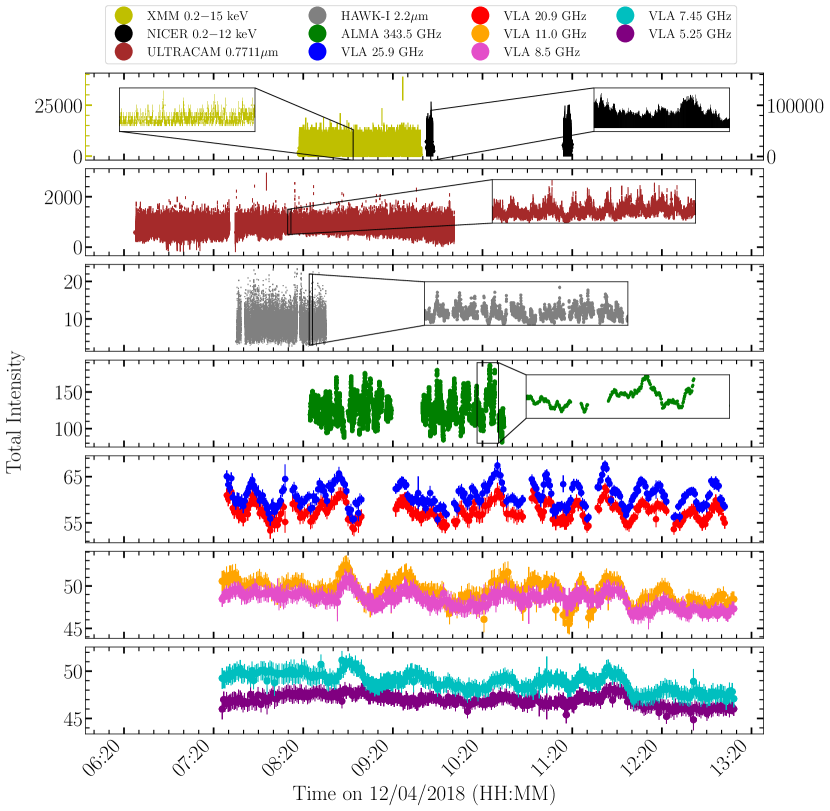
Figure 1: Simultaneous multi-band light curves of the BHXB MAXI J1820+070 taken on 2018 April 12 in the X-ray (XMM-Newton 0.2–15 keV and NICER 0.2–12 keV), optical (0.7711$\mu$m), infrared (2.2$\mu$m), sub-mm (343.5 GHz), and radio (5.25–25.9 GHz) bands. The main panels from top to bottom show light curves for progressively decreasing electromagnetic frequency bands, and the inset panels show zoomed in versions of the light curves. The total intensity units for VLA/ALMA are mJy/bm, HAWK-I is amplitude with respect to the reference star, ULTRACAM is arbitrary instrumental units, and NICER/XMM-Newton are counts/sec. The time resolution for the VLA, ALMA, HAWK-I, ULTRACAM, NICER, and XMM-Newton light curves are: 5 sec, 2 sec, 0.0625 sec, 0.01 sec, 0.01 sec, and 0.004 sec, respectively. We observe clear variability in the emission from MAXI J1820+070, taking the form of rapid flaring across all of the electromagnetic bands sampled.

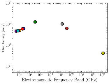
Figure 2: Time-averaged broad-band spectrum of our radio–X-ray data of MAXI J1820+070 (see Table 1 and §2.3, 2.4, 2.5). The colours of the data points correspond to the same colours of the electromagnetic frequency bands in Figure 1. The radio through sub-mm data appear to lie on the slightly inverted optically thick portion of the jet spectrum (spectral index $\alpha_{\rm thick}\sim 0.25$), while the infrared and optical data appear to lie on the steep optically thin portion of the jet spectrum (spectral index $\alpha_{\rm thin}\sim-0.5$).

2.2 VLA radio observations

MAXI J1820+070 was observed with the Karl G. Jansky Very Large Array (VLA; Project Code: 18A-470) on 2018 April 12, for a total on-source observation time of 6.0 hours. The array was in the A configuration at the time of our observations, where we split the full array into 3 sub-arrays of 10, 9, and 8 antennas. Observations in each sub-array were made with the 8-bit samplers, where each sub-array observed exclusively in one frequency band; C (4 – 8 GHz), X (8 – 12 GHz), or K (18 – 26 GHz) band. Each band was comprised of 2 base-bands, with 8 spectral windows of 64 2-MHz channels each, giving a total bandwidth of 1.024 GHz per base-band. The sub-array setup allows us to push to shorter correlator dump times than would be possible if we were using the full array. In these observations, we set a 0.15-second correlator dump time, providing the highest time resolution possible, while staying within the standard 25 ${\rm Mb\,s}^{-1}$ data rate limit. With our sub-array setup, we record data fast enough to probe timescales down to hundreds of ms. We implemented a custom non-periodic target/calibrator cycle for each sub-array, alternating observing MAXI J1820+070 and calibrators, at one band per sub-array, such that we obtained simultaneous data in all three bands. We reduced and imaged the data within casa, using standard procedures outlined in the casaGuides for VLA data reduction (i.e., a priori flagging, setting the flux density scale, initial phase calibration, solving for antenna-based delays, bandpass calibration, gain calibration, scaling the amplitude gains, and final target flagging). We used 3C286 (J1331+305) as a flux/bandpass calibrator, and J1824+1044 as a phase calibrator. To obtain high time resolution flux density measurements, we follow the same procedure as for the ALMA data, using our custom casa variability measurement scripts. We performed phase-only self-calibration (down to a solution interval of 10 sec) prior to running the imaging scripts. To check that any variability observed in these MAXI J1820+070 radio frequency light curves is dominated by intrinsic variations in the source, and not due to atmospheric or instrumental effects, we also ran additional tests on a check source (see Appendix LABEL:sec:ap_cal for details). An time-averaged flux density measurement over the whole observation period is shown for each band in Table 1.

2.3 VLT HAWK-I infrared observations

HAWK-I is a wide-field photometer operating in the near-IR band (0.97 to 2.31 $\mu$m) made by four HAWAII 2RG 2048x2048 pixel detectors (Pirard2004). High time resolution near-IR ($K_{s}$ band; $2.2\mu$m; $1.4\times 10^{5}$ GHz) data of MAXI J1820+070 was collected on 2018 April 12 between 07:32:58 – 08:31:39 UTC with the HAWK-I instrument mounted on the Very Large Telescope (VLT; Project Code: 0100.D-0308(A)) UT-4/Yepun. The instrument was set up in Fast-Phot mode: i.e. the detector was limited only to a stripe made of 16 contiguous windows of 64 $\times$ 64 pixels in each quadrant, permitting a time resolution of 0.0625 sec. In order to read out the data, the final light curve has periodic gaps of $\approx$ 3 sec every 15–16 sec. We pointed the instrument in order to place the target and a bright reference star (K${}_{s}$= 11.9) in the lower-left quadrant (Q1). We extracted photometric data using the ULTRACAM data reduction pipeline v9.14 tools (dhilon2007), deriving the parameters from the bright reference star and its position (the position of the target was linked in each exposure). To avoid seeing effects, we used the ratio between the source and the reference star count rate. Finally, we put the time of each frame in the Barycentric Dynamical Time (BJD_TDB) system. We also derive a rough estimate of the time-averaged flux density from these data, to help put our longer wavelength measurements into context, by comparing the target to the reference star. With $E(B-V)=0.18$ (tuck18), this leads to a de-reddened flux density of $\sim 101$ mJy.

2.4 NTT ULTRACAM optical observations

ULTRACAM is a fast-timing optical instrument which uses three channels for simultaneous multi-wavelength monitoring, and can observe at a high frame rate (dhilon2007). High time resolution optical ($i_{s}$ band; $0.7711\mu$m; $3.9\times 10^{5}$ GHz) data of MAXI J1820+070 was collected on 2018 April 12 between 06:28 – 10:01 UTC with the ULTRACAM instrument mounted on the 3.5 m New Technology Telescope in La Silla, Chile (NTT; Project Code: 0101.D-0767). The instrument was used in two-window mode (one each for the target and the comparison star), with both window sizes of 50 $\times$ 50 pixels with a 2 $\times$ 2 binning for sensitivity, and speed at 96.5 Hz in $i_{s}$ band (using ULTRACAM’s ‘co-adding’ feature, $i_{s}$ band was observed with an exposure time of 8.96 ms, and a total cycle time of 10.4 ms, giving 1.44 ms of dead time and a sampling rate of $\sim$96.5 Hz).

The data were reduced using the ULTRACAM pipeline v9.14 (dhilon2007). The bias was subtracted from each frame, and flat field corrections were also applied. Aperture sizes scaled to the instantaneous seeing were used, with radii between 0.7$\arcsec$ and 3.5$\arcsec$, with an annulus of between 12$\arcsec$ and 6.3$\arcsec$ to calculate the background. These apertures had variable centre positions that tracked the centroids of the sources on each frame, with a two-pass iteration (where an initial pass is made to track the sources on the CCD before a second photometry pass) used for accuracy. Our times were then adjusted to BJD_TDB system using methods given in eastman_achieving_2010.

Our comparison star is listed as PSO J182026.430+071011.742 in the PanSTARRS survey catalog (Magnier_PanSTARRS_2020). We extracted the target count rates and count rates for the comparison star using aperture photometry with a variable aperture size dictated by the seeing conditions. The aperture also tracked the centroid of the source of interest by using a bright star in the field as a reference source. We also derive a rough estimate of the time-averaged flux density from these data, to help put our longer wavelength measurements into context, by comparing the target to the reference star. With $E(B-V)=0.18$ (tuck18), this leads to a de-reddened flux density of $\sim 62$ mJy.

2.5 NICER and XMM-Newton X-ray observations

Table 1: Time-averaged radio and sub-mm flux densities of MAXI J1820+070

Electromagnetic	Average Flux	Systematic
Frequency Band	Density (mJy)${}^{\dagger}$	Error (%)${}^{\star}$
5.25 GHz	$46.0\pm 0.1$	5
7.45 GHz	$48.1\pm 0.2$	5
8.5 GHz	$48.3\pm 0.2$	5
11.0 GHz	$49.2\pm 0.2$	5
20.9 GHz	$58.7\pm 1.1$	10
25.9 GHz	$60.5\pm 1.1$	10
343.5 GHz	$125.3\pm 0.05$	5

${}^{\dagger}$ Errors on the VLA and ALMA average flux density measurements are calculated from the local rms in images made from data taken over the entire observation period.

${}^{\star}$ Additional systematic errors added (in quadrature) to the average flux density error measurements, to account for absolute flux calibration uncertainties at the VLA and ALMA.

NICER (Neutron star Interior Composition ExploreR) is an X-ray instrument aboard the International Space Station (ISS). It comprises 52 functioning X-ray concentrator optics and silicon drift detector pairs, arranged in seven groups of eight. Individual photons between 0.2–12 keV, and their energies, can be detected to a time resolution of 40 ns (GendreauArzoumanian_NICER_2016).

For this work, we reduced NICER data from ObsID 1200120127 using nicerdas, a collection of NICER-specific tools which is apart of the heasarc software package. Full Level2 calibration and screening was conducted with the nicerl2 task, which calibrated, checked the time intervals, merged, and cleaned the data. Barycentric correction was carried out using barycorr.

XMM-Newton observed MAXI J1820+070 with the EPIC-pn camera for approximately 2 hours, between 07:39:28 – 9:39:28 UTC on 2018 April 12. These observations were set up in Burst Mode. Events were extracted with a PATTERN <= 4, FLAG==), in the 0.2–15 keV energy range. We used a box of angular size $\approx$ 86 arcsec (RAWX between 28 and 48). The event file was barycentred using the command barycen, and the XMM-Newton X-ray light curve was extracted with 1 ms time resolution. Due to the very high count rate, the source showed several telemetry drop outs lasting $\approx$ 14 sec every $\approx$ 30–50 sec.

To acquire a rough estimate of the X-ray flux, for comparison with our other multi-wavelengths measurements, we fit the XMM-Newton X-ray spectrum with a powerlaw $+$ diskbb model, finding an X-ray flux in the $1-10$ keV band of $\sim 4.9\times 10^{-8}\,{\rm erg\,cm}^{-2}{\rm s}^{-1}$ ($\sim 4$ mJy).

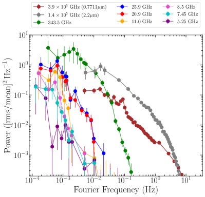
Figure 3: Fourier power spectra (PSDs) of optical (0.7711$\mu$m; ULTRACAM), infrared (2.2$\mu$m; HAWK-I), sub-mm (343.5 GHz; ALMA) and radio (5.25 – 25.9 GHz; VLA) emission from MAXI J1820+070. Note that PSDs of the X-ray bands are shown separately in Figure 4 for clarity. The PSDs shown here were built by stitching together PSD segments created from data imaged/extracted with different time-bin sizes (with the shortest time-scales sampled being 0.01/0.065/2/5 sec for the optical/infrared/sub-mm/radio bands; see §3.2 for details), in order to circumvent the gaps in the light curves and sample the lower Fourier frequencies. In these PSDs, we observe a clear trend in the shape of the PSDs with electromagnetic frequency band, where the break in the PSDs moves to lower Fourier frequencies as we shift to lower electromagnetic frequency bands. Note that all PSDs shown here have been white-noise subtracted, and the pre-white noise subtracted PSDs are shown in Appendix LABEL:sec:ap_wn.

3 Measuring jet timing characteristics

3.1 Light curves

Time-resolved multi-band light curves of MAXI J1820+070 are displayed in Figure 1 and an average broad-band spectrum is displayed in Figure 2. In the light curves, we observe clear structured variability at all electromagnetic frequencies, in the form of multiple flaring events. Similar flare morphology can be observed between the time-series signals (especially in the radio and sub-mm bands), suggesting that the emission in the different electromagnetic frequency bands is correlated and may show measurable delays. Upon comparing the signals across all of the electromagnetic bands sampled, the variability appears to occur on much faster timescales in the higher electromagnetic bands when compared to the lower electromagnetic bands. When considering the radio and sub-mm bands, the variability is of higher amplitude in the higher frequency sub-mm band ($\sim 100$ mJy), when compared to the lower frequency radio bands ($\sim 5-20$ mJy). Further, the sub-mm band shows a higher average flux level when compared to the radio bands ($\sim 125$ mJy in the sub-mm vs. $\sim 46-60$ mJy in the radio bands; see Table 1), indicating an inverted optically thick radio through sub-mm spectrum. The infrared and optical bands appear to not lie on the extension of the radio–sub-mm spectrum, but rather on the steep optically thin portion of the jet spectrum, indicating the jet spectral break lies between the sub-mm and infrared bands (see Figure 2). This result is consistent with previous reports of bright mid-IR emission in excess of the optical emission during the hard state of the outburst (ateldrus1820). All of these emission patterns are consistent with the radio, sub-mm, infrared, and optical emission originating in a compact jet, where the higher electromagnetic frequency emission is emitted from a region closer to the black hole (with a smaller cross-section), while the lower electromagnetic frequency emission is emitted from regions further downstream in the jet flow (with larger cross-sections).

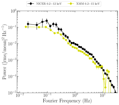
Figure 4: Fourier power spectra (PSDs) of the NICER and XMM-Newton X-ray emission from MAXI J1820+070. Note that the X-ray PSDs shown here have been white-noise subtracted, and the pre-white noise subtracted PSDs are shown in Appendix LABEL:sec:ap_wn.

3.2 Fourier Power Spectra

To characterize the variability we observe in the light curves of MAXI J1820+070, we opted to perform a Fourier analysis on the data. We use the stingray software package for this Fourier analysis (stingray; stingray2), and Figures 3 and 4 display the resulting power spectral densities (PSDs).

As our light curves contain gaps, to build the PSDs over a wide range of Fourier frequencies we stitch together PSD segments created from light curves imaged/extracted with different time-bin sizes. In particular, by building light curves on timescales larger than the gaps, we can manufacture a continuous time-series with which we are able to probe a lower Fourier frequency range. For the radio frequency VLA data, we use three PSD segments, built from light curves with 5 sec (final PSD segment is an average over 100 sec chunks), 60 sec (final PSD segment is an average over 15 min chunks), and 240 sec (final PSD segment is an average over 90, 108, 132 min chunks for 20.9/5.9GHz, 8.5/11 GHz, 5.25/7.45 GHz bands, respectively) time-bins. For the sub-mm frequency ALMA data, we use two PSD segments, built from light curves with 2 sec (final PSD segment is an average over 180 sec chunks) and 90 sec (final PSD segment is an average over 50 min chunks) time-bins. For the infrared/optical frequency data, we use two PSD segments, built from light curves with 0.0625/0.01 sec (final PSD segment is an average over 15/0.75 sec chunks) and 10/0.5 sec (final PSD segment is an average over 200 sec chunks for both) time-bins. For the NICER/XMM-Newton X-ray frequency data, we use only one PSD segment, built from light curves with 0.01/0.004 sec time-bins (final PSD segment is an average over 50/30 sec chunks). The number of segments/chunk sizes were chosen based on the gap timescales, and to reduce the noise in the PSDs. Further, a geometric re-binning in frequency was applied (factor of $f=0.2$ for radio–sub-mm, $f=0.05$ for infrared/optical, and $f=0.15$ for X-ray, where each bin-size is $1+f$ times larger than the previous bin size) to reduce the scatter at higher Fourier frequencies in all the PSDs. The PSDs are normalized using the fractional rms-squared formalism (bel90), and white noise has been subtracted. White noise levels were estimated by fitting a constant to the highest Fourier frequencies (see Appendix LABEL:sec:ap_wn).

The PSDs all appear to display a broken power-law type form, where the highest power occurs at the lowest Fourier frequencies (corresponding to the longest timescales sampled). However, there are clear differences between the PSD shape for the different bands, where the break in the PSDs moves to lower Fourier frequencies as we shift to lower electromagnetic frequency bands. The same effect can be seen when examining the smallest time-scales (or highest Fourier frequencies) at which significant power is observed in each band (i.e., 10 sec at 343.5 GHz, 100 sec at 20.9/25.9 GHz, and 500 sec at 5.25–11 GHz). This is the first time an evolving PSD with electromagnetic frequency has been observed from a BHXB.

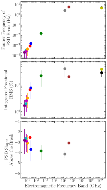
Figure 5: Variability characteristics of the emission from MAXI J1820+070, derived from the PSDs shown in Figure 3 & 4. From top to bottom, the panels show the Fourier frequency of the PSD break, integrated fractional RMS, and the slope above the PSD break (as we only fit the X-ray PSDs with Lorentzian components, no PSD slope is shown for these bands). The colours of the data points in all panels correspond to the same colours of the electromagnetic frequency bands in Figure 3 & 4. We observe a clear trend with electromagnetic frequency in all of these quantities, except for the slope above the PSD breaks, which remains relatively constant (within error) across the radio–optical bands.

Table 2: PSD modelling results

Electromagnetic Frequency Band	$\bm{f_{\rm break}}$ (Hz) ${}^{\dagger}$	Slope above break	$\bm{z_{\nu}}$ ($\bm{\times 10^{12}}$ cm)${}^{\star}$	$\bm{z_{\rm cross}}$ ($\bm{\times 10^{11}}$ cm)${}^{\ddagger}$
5.25 GHz	$(2.0^{+2.1}_{-0.8})\times 10^{-4}$	$-2.84^{+1.09}_{-1.34}$	$37.6^{+32.7}_{-19.0}$	$2.8^{+2.9}_{-1.5}$
7.45 GHz	$(3.1^{+2.6}_{-2.2})\times 10^{-4}$	$-2.67^{+0.65}_{-0.89}$	$22.2^{+33.4}_{-11.2}$	$1.7^{+2.8}_{-0.9}$
8.5 GHz	$(2.8^{+3.5}_{-1.4})\times 10^{-4}$	$-2.93^{+0.70}_{-1.04}$	$26.7^{+30.1}_{-15.0}$	$2.0^{+2.8}_{-1.2}$
11.0 GHz	$(4.1^{+3.2}_{-2.6})\times 10^{-4}$	$-3.12^{+0.79}_{-0.94}$	$17.8^{+22.9}_{-8.6}$	$1.4^{+1.9}_{-0.7}$
20.9 GHz	$(8.6^{+4.9}_{-9.9})\times 10^{-4}$	$-2.57^{+0.71}_{-1.12}$	$9.1^{+10.6}_{-3.8}$	$0.8^{+1.0}_{-0.4}$
25.9 GHz	$(1.5^{+0.9}_{-0.6})\times 10^{-3}$	$-3.72^{+0.87}_{-1.14}$	$5.2^{+4.2}_{-2.1}$	$0.4^{+0.4}_{-0.2}$
343.5 GHz	$(1.5^{+0.7}_{-0.5})\times 10^{-2}$	$-3.87^{+0.55}_{-0.87}$	$0.5^{+0.3}_{-0.2}$	$0.05^{+0.04}_{-0.02}$
$2.2\mu$m	$2.7^{+0.4}_{-0.3}$	$-4.18^{+0.34}_{-0.39}$	$(2.9^{+0.8}_{-0.6})\times 10^{-3}$	$(2.3^{+1.0}_{-0.8})\times 10^{-4}$
$0.7711\mu$m	$5.8^{+0.8}_{-0.5}$	$-3.10^{+0.22}_{-0.22}$	$(1.3^{+0.3}_{-0.2})\times 10^{-3}$	$(1.2^{+0.5}_{-0.4})\times 10^{-4}$
NICER 0.2–12 keV	$4.9^{+0.4}_{-0.4}$	…	…	…
XMM-Newton 0.2–15 keV	$4.7^{+0.8}_{-0.7}$	…	…	…

${}^{\dagger}$ For the NICER/XMM-Newton X-ray PSDs, we take the break frequency to be the “characteristic frequency" defined in belloni02 as $f_{\rm break}=\sqrt{\nu_{0}^{2}+\Delta^{2}}$, where $\nu_{0}$ is the central frequency and $\Delta$ is the FWHM of the highest Fourier frequency Lorentzian.

${}^{\star}$ Distance downstream from the black hole to the $\tau_{\nu}=1$ surface. Here we use the formalism, $z_{\nu}=\frac{\beta c\delta}{f_{\rm\,break}}$, and sample from the best-fit $\beta$ distribution along with the known $\theta$ distribution (see §3.2 and LABEL:sec:model for details).

${}^{\ddagger}$ Jet cross-section assuming a conical jet. Here we use the formalism, $z_{\rm cross}=z_{\nu}\tan{\phi}$, and sample from the best-fit $\phi$ distribution (see §LABEL:sec:model for details).