On the exponentially small corrections
to ${\cal N}=2$ superconformal correlators at large R-charge

Simeon Hellerman^1,2

¹Kavli Institute for the Physics and Mathematics of the Universe (wpi)
The University of Tokyo
Kashiwa, Chiba 277-8582, Japan
²Department of Physics, Faculty of Science,
University of Tokyo, Bunkyo-ku, Tokyo 133-0022, Japan

Abstract

In this note we consider Coulomb-branch chiral primary correlation functions in ${\cal N}=2$ superconformal QCD with gauge group $SU(2)$, in the limit of large R-charge ${\color[rgb]{0.808594,0.242188,0.46875}{{\cal J}}}=2n$ for the chiral primary operators $[{\cal O}(x)]^{n}$ with the inverse gauge coupling $\tau$ held fixed. In previous work [5, 6, 7, 8] these correlation functions were determined to all orders in $n$, up to unknown exponentially small corrections. In this paper we determine the first several orders of the asymptotic expansion of the exponentially small correction itself. To do this we use: the physical interpretation of the exponentially small correction as the virtual propagation of a massive BPS particle, to fix the leading term in the expansion; the supersymmetric recursion relations of [68, 67, 3, 14] to derive differential equations for the coupling-dependence of the subleading terms; and the double-scaling limit of [9, 13], to fix undetermined coefficients in the solution of the differential equation. We calculate the expansion of the exponentially small term up to and including relative order $n^{-{5\over 2}}$. We also use the recursion relations to calculate the subleading large-${\color[rgb]{0.808594,0.242188,0.46875}{{\cal J}}}$ corrections to the exponentially small correction in the double-scaling limit, up to and including relative order $n^{-5}$ at fixed double-scaled coupling ${\color[rgb]{0.808594,0.242188,0.46875}{\lambda}}$. We compare the expansion to exact results from supersymmetric localization [91] at the coupling $\tau={{25}\over\pi}\,i$, up to $n=150$. At values $n\sim 100-150$, we find the fixed-coupling and double-scaled large-R-charge expansions are accurate to within one part in $10^{6}$ and $10^{8}$, respectively, of the size of the exponentially small correction itself. Relative to the full correlator including the dominant eft contribution, these estimates give results accurate to one part in $10^{15}$ and $10^{17},$ respectively.

Dedication

This paper is dedicated to the memory of Fred Hellerman, and to his granddaughter Dymond Henry on the occasion of her thirteenth birthday.

Contents

1. 1 Introduction
2. 2 Review of chiral primary correlation functions for ${\cal N}=2$ superconformal theories in $D=4$ with one-dimensional Coulomb branch
   1. 2.1 Large R-charge expansion at fixed coupling
   2. 2.2 Scheme-dependence and marginal couplings
   3. 2.3 The case of ${\cal N}=2$ superconformal QCD with $G=SU(2)$ and $N_{{\rm{F}}}=4$
   4. 2.4 Large R-charge in the double-scaling limit
   5. 2.5 Large-charge, fixed $\tau$ limit, versus the large-${\color[rgb]{0.808594,0.242188,0.46875}{\lambda}}$ limit of the double-scaling limit
3. 3 Large-R-charge asymptotic expansion for the massive macroscopic propagation function $q_{n}^{({\rm{\textsc{mmp}}})}$ at fixed $\tau$
   1. 3.1 Recursion relations for subleading large-charge corrections at fixed $\tau$
   2. 3.2 Fixing the integration constants using the strong coupling expansion of the double-scaling limit
4. 4 Accuracy of the asymptotic estimates of the MMP function at large $n$ and fixed $\tau$
   1. 4.1 Limitations on the accuracy of agreement between the fixed-$\tau$ large-charge asymptotic series and the localization calculation
   2. 4.2 Summary and highlights of the results
   3. 4.3 Plots
      1. 4.3.1 On the visual display of quantitative information
      2. 4.3.2 Plotting the log of relative error of the fixed-$\tau$ estimates through order $n^{-{5\over 2}}$ in the exponent, evaluated at $\tau={{25}\over\pi},1\leq n\leq 150.$
      3. 4.3.3 Plotting the log of relative error of the fixed-$\tau$ estimates through order $n^{-{5\over 2}}$ in the exponent, evaluated at $\tau={{25}\over\pi},1\leq n\leq 150.$, relative to the full log of the scheme-independent correlator $\tilde{G}_{2n}\equiv{{G_{2n}}\over{(G_{2})^{n}}}=e^{q_{n}-n\,q_{1}+(n-1)q_{0}}$
   4. 4.4 Table of values of the fixed-$\tau$ large-charge asymptotic estimates at $\tau={{25}\over\pi}\,i$, up to $n=150$
   5. 4.5 Table of effective digits of accuracy of the fixed-$\tau$ large-charge asymptotic estimates at $\tau={{25}\over\pi}\,i$, up to $n=150$
5. 5 Subleading large-$n$ corrections to the double-scaling limit
   1. 5.1 Recursion relation for the two-loop correction
   2. 5.2 Solving the recursion relation for the two-loop correction
   3. 5.3 Physical interpretation of the double-scaled MMP term at order $n^{-1}$
      1. 5.3.1 Breakdown of the double-scaling regime at ultra-large $n$
      2. 5.3.2 Physical mechanism for the breakdown of double-scaled perturbation theory
      3. 5.3.3 Higher order in $n$
   4. 5.4 Order $n^{-2}$ through $n^{-5}$ corrections to the MMP function at fixed ${\color[rgb]{0.808594,0.242188,0.46875}{\lambda}}$
6. 6 Accuracy of the asymptotic large-charge expansion at large $n$ and fixed double-scaled coupling ${\color[rgb]{0.808594,0.242188,0.46875}{\lambda}}$
   1. 6.1 Limitations on the accuracy of agreement between the asymptotic series and the localization calculation
   2. 6.2 Plotting the log of relative error of the double-scaled estimates through order $n^{-5}$ at fixed ${\color[rgb]{0.808594,0.242188,0.46875}{\lambda}},$ evaluated at $\tau={{25}\over\pi},1\leq n\leq 150$
   3. 6.3 Table of values of the double-scaled (i.e. fixed-${\color[rgb]{0.808594,0.242188,0.46875}{\lambda}}$) large-charge asymptotic estimates at $\tau={{25}\over\pi}\,i$ up to $n=150$
   4. 6.4 Tables listing the accuracy of the double-scaled (i.e. fixed-${\color[rgb]{0.808594,0.242188,0.46875}{\lambda}}$) large-charge asymptotic estimates at $\tau={{25}\over\pi}\,i$, up to $n=150$
7. 7 Discussion and conclusions

1 Introduction

Recently there has been development of the use of large quantum number as a limit in which observables can be computed in systems with global symmetries with control over quantum effects beyond the usual weak-coupling regime. In systems with no weak-coupling parameter in the Hamiltonian, inverse large quantum number can play the role of a small coupling constant [15, 16, 17, 18, 19, 20, 21, 22, 23, 24, 25, 37, 26, 27, 30, 31, 32, 33, 35, 41, 42, 29, 28, 38, 39, 40, 44, 45, 46, 81, 83, 84, 90, 85, 86, 87, 88, 89, 80, 82, 94, 5, 9, 6, 10, 11, 12, 13, 7, 8] In a wide range of systems one finds that the limit of large quantum number dramatically simplifies the computation of many observables in the theory, while preserving interesting dynamical behaviors of the theory. In all examples, the physical picture is rather straightforward: The large-charge state is well-described by a classical ground state of a set of Nambu-Goldstone degrees of freedom  [15, 16, 17, 37, 26, 27, 30, 31, 32, 33, 35, 34, 36]. In such theories, quantum fluctuations about the dominant classical solution are suppressed by negative powers of the total charge ${\color[rgb]{0.808594,0.242188,0.46875}{{\cal J}}}$. In principle this picture gives an all-orders asymptotic expansion in inverse powers of the charge for operator dimensions, OPE coefficients, and other large-charge observables. The only unknown ingredients are the Wilson coefficients in the action of the large-charge eft. Beyond an all-orders asymptotic expansion, the eft picture is modified only by exponentially small corrections associated with virtual propagation of massive non-Goldstone degrees of freedom over distances of order the infrared scale.

One particularly nice testing ground for these ideas has been superconformal field theory in $D=4$ with ${\cal N}=2$ extended supersymmetry. [5, 9, 6, 10, 11, 12, 13, 7, 8], particularly those with a one-complex-dimensional Coulomb branch. For such theories there are tools available associated with exact supersymmetry that allow the computation of supersymmetrically-protected observables at a nonperturbative level, with the computation of the $S^{4}$ partition function as a starting point. These methods [14], associated with supersymmetric localization [47, 48, 49] make it possible to check the predictions of the large-quantum-number expansion against an independent calculation.

For $D=4,~{}{\cal N}=2$ superconformal theories, the simplest nontrivial large quantum number calculation is the two-point function of a BPS chiral primary operator carrying large $U(1)_{R}$ R-charge. For the special case of rank-one gauge group $G=SU(2)$, the chiral ring of the Coulomb branch is generated by a single operator ${\cal O}_{\Delta}$ of dimension $\Delta$ and $U(1)_{{\rm{R}}}$ R-charge $J=\Delta$. In previous work [5, 6, 7, 8] the correlation functions of the $n^{\rm{\underline{th}}}$ powers of these operators have been computed in a large-$n$ expansion. In the expansion at large $n$ with the coupling held fixed, there is a simple asymptotic formula for the logarithm of the correlation function that holds to all orders in ${1\over n}$, and gives universal, theory-independent predictions for all power-law terms ${\color[rgb]{0.808594,0.242188,0.46875}{{\cal J}}}^{-k},~{}k\geq 1$ down to corrections exponentially small in $\sqrt{{\color[rgb]{0.808594,0.242188,0.46875}{{\cal J}}}}$. These exponentially small corrections are the leading non-universal scheme-independent contributions to the log of the correlation function, and represent the contribution of virtual macroscopic propagation of BPS particles which are massive on the Coulomb branch. Their masses scale as $\sqrt{{\color[rgb]{0.808594,0.242188,0.46875}{{\cal J}}}}$ because the theory is conformal, so their masses come purely from the expectation value of the vector multiplet scalar $a$ which is in turn set by the R-charge density in the classical solution describing the charged ground state. Concrete formulae for those relationships were given in [8] and will be reviewed in sec. 2.5.

These massive macroscopic propagation (mmp) corrections are interesting, and we would like to study them in order to probe the physics associated with these tiny but distinctly visible corrections, and also to increase the numerical precision of the large-R-charge expansion. In the case of non-Lagrangian theories such as Argyres-Douglas theories [71, 72, 73, 74, 75, 76, 77] we do not yet have the tools to compute these corrections. The two interacting Lagrangian superconformal theories in $D=4$ with ${\cal N}=2$ supersymmetry, are both $G=SU(2)$ gauge theories: ${\cal N}=4$ super-Yang-mills, and superconformal QCD with $4$ hypermultiplets in the fundamental representation. In the case of ${\cal N}=4$ super-Yang-Mills, the MMP corrections vanish. In this paper we will give asymptotic formulae for the leading large-$n$ asymptotics of the massive macroscopic propagation term, in the case of ${\cal N}=2$ superconformal QCD (sqcd) with $G=SU(2)$ and $N_{{\rm{F}}}=2N_{{\rm{c}}}=4$.

The plan of the paper is as follows. In sec. 2 we will review relevant material on chiral primary correlation functions for ${\cal N}=2$ superconformal theories in $D=4$ with one-dimensional Coulomb branch In sec. 3 we will apply the recursion relations of [68, 67, 3, 14] to the formula for the exponentially small correction $q_{n}^{({\rm{\textsc{mmp}}})}$, which will give an order by order differential equation for the coupling-dependence of each order of the large-$n$ expansion of $q_{n}^{({\rm{\textsc{mmp}}})}$. We will find it is algorithmic to solve this equation in closed form up to a single undetermined term $c_{p}({\rm Im}[\sigma]/n)^{{p\over 2}}$ in the logarithm of $q_{n}^{({\rm{\textsc{mmp}}})}$ at each order $p$. By taking the double-scaling limit, we will see that we can determine the coefficient $c_{p}$ precisely by matching it with a term in the large-${\color[rgb]{0.808594,0.242188,0.46875}{\lambda}}$ expansion of the logarithm of the function $F^{{\rm{inst}}}[{\color[rgb]{0.808594,0.242188,0.46875}{\lambda}}]$ appearing in [13]. We carry out this algorithm to give the fixed-coupling, large-$n$ corrections to the exponentially small correction up to $p=5,$ the term of order $n^{-{5\over 2}}$ in the exponent. In sec 4 we will test our subleading large-$n$ corrections by comparison with high-precision numerical data representing the output of the algorithm of [14] at one particular value of the complexified gauge coupling ($\tau={{25}\over\pi}\,i$) and large values of $n$. At this value of $\tau$ and large $n,$ we find highly precise agreement between the exact results from localization on the one hand, and the large-R-charge expansion of the exponentially small correction on the other hand. Even at small values of the R-charge $n=1,2,3\cdots,$ we find startlingly precise agreement between the exact result and the large-R-charge asymptotic estimate.

In sec. 5 we will apply the recursion relations directly to find the subleading large-$n$ corrections in the double-scaling limit, and solve for the subleading large-$n$ corrections to the double-scaling limit up to and including the six-loop contribution to the MMP term, which is order $n^{-5}$ at fixed ${\color[rgb]{0.808594,0.242188,0.46875}{\lambda}}$. We will show that the large-${\color[rgb]{0.808594,0.242188,0.46875}{\lambda}}$ limit of each order in the expansion has an increasing power-law growth at large ${\color[rgb]{0.808594,0.242188,0.46875}{\lambda}}$ on top of the exponential suppresson, which explains why there is a distinction between the large-${\color[rgb]{0.808594,0.242188,0.46875}{\lambda}}$ expansion of the double-scaling limit on the one hand, and the large-$n$ expansion at fixed $\tau$ on the other hand. We will show that the large-${\color[rgb]{0.808594,0.242188,0.46875}{\lambda}}$ growth of the subleading large-$n$ corrections to the double scaling limit, are all directly connected with the ${\cal N}=2$ one-loop threshold correction to the effective Abelian gauge coupling [57, 56, 49] that gives the entire perturbative difference between the UV coupling $\tau$ and the effective IR coupling $\sigma\simeq 2\tau+{{4i}\over{\pi}}\,{\tt log}[2]$. Then in sec 6 we go on to compare the data with our subleading large-$n$ corrections to the double-scaled amplitude. Finally we comment on some outstanding issues in the conclusions (sec. 7), including the possible large-order behavior of the asymptotic series in $1\over{\sqrt{n}}$ and its physical interpretation [94]

2 Review of chiral primary correlation functions for ${\cal N}=2$ superconformal theories in $D=4$ with one-dimensional Coulomb branch

2.1 Large R-charge expansion at fixed coupling

In the special case of Lagrangian superconformal $SU(2)$ gauge theories with marginal coupling constant, the chiral ring generator has dimension and R-charge $\Delta=J=2$ and its Lagrangian representation is ${\cal O}\propto{\rm Tr}[\hat{\phi}^{2}]$ where $\hat{\phi}$ is the lowest component of the adjoint-valued $SU(2)$ gauge vector multiplet superfield. In Lagrangian and non-Lagrangian theories alike, if the gauge symmetry is rank one, the Coulomb branch has complex dimension $1$ and its chiral ring is spanned by the operators ${\cal O}_{\Delta}^{n}$ for $n=0,1,2,\cdots$. The correlation functions

$$\begin{array}[]{c}G_{2n}\equiv|x-y|^{+2\Delta}\,\langle{\cal O}^{n}_{\Delta}(x)\,\overline{{\cal O}}^{n}_{\Delta}(y)\rangle\end{array}$$ (2.2)

are special observables of the theory that are particularly robust, because they are unaffected by any possible $D-$term deformations of the theory; they are related to special supersymmetrically protected properties of the theory, and can be calculated [68, 67, 3, 14] via supersymmetric localization [47, 48, 49]

At large $n$ the R-charge ${\color[rgb]{0.808594,0.242188,0.46875}{{\cal J}}}\equiv n\Delta$ carried by these operators, is large, and one can use the large-charge eft to calculate the asymptotic expansion of the correlation function $G_{2n}$ at large $n$. For Lagrangian and non-Lagrangian theories alike, one finds

$$\begin{array}[]{c}G_{2n}=2^{{+2n\Delta}}\,[Z_{S^{4}}]^{-1}\,{\rm exp}\{q_{n}\}\ ,\end{array}$$ (2.4)

$$\begin{array}[]{c}q_{n}\equiv q_{n}^{({\rm{\textsc{eft}}})}+({\rm exponentially~{}small~{}at~{}large~{}}n)\ ,\end{array}$$ (2.6)

$$\begin{array}[]{c}q_{n}^{({\rm{\textsc{eft}}})}\equiv An+B+{\rm log}\big{[}\Gamma[n\Delta+\alpha+1]\big{]}\end{array}$$ (2.8)

where $Z_{S^{4}}$ is the four-sphere partition function, $A$ and $B$ may depend on the theory and on the marginal parameters if any, and $\alpha$ is a coefficient proportional to the Weyl $a-$anomaly mismatch between the interacting CFT and the effective theory of the Coulomb branch. The $\alpha-$coefficient can be expressed convention-independently in terms of the $a-$anomaly coefficient $a_{{\rm{favm}}}$ of a free $U(1)$ vector multiplet:

$$\begin{array}[]{c}\alpha={5\over{12}}\,{{a_{{\rm{CFT}}}-a_{{\rm{\textsc{eft}}}}}\over{a_{{\rm{favm}}}}}\ .\end{array}$$ (2.10)

A table of $\alpha$ coefficients of all known rank-one ${\cal N}=2$ superconformal theories was given in [5]. For ${\cal N}=4$ super-Yang-Mills theory the value of $\alpha$ is $+1$; for the case we will principally study in this paper, ${\cal N}=2$ superconformal QCD with $N_{{\rm{F}}}=4,$ the value of $\alpha$ is $+{3\over 2}$.

2.2 Scheme-dependence and marginal couplings

The $A$ and $B$ coefficients also depend on the normalization of the chiral ring generator and on the marginal coupling if any, and also, relatedly, on scheme choices. When there is a marginal coupling $\tau,$ the chiral ring generator lies in the same supermultiplet as the marginal operator, whose normalization and phase transform as holomorphic cotangent vectors under reparametrizations of the holomorphic coupling $\tau$; so we define ${\cal O}\equiv{\cal O}_{[{\tau}]}$ with a (sometimes implicit) lower index $\tau$ to indicate its transformation under reparametrizations of the holomorphic coupling constant,

$$\begin{array}[]{c}{\cal O}_{[{\tau}]}={{d\tau^{\prime}}\over{d\tau}}\,{\cal O}_{[{\tau^{\prime}}]}\ .\end{array}$$ (2.12)

It follows from the definition of $A$ that $A$ also transforms under holomorphic reparametrizations, as the logarithm of the norm-squared of a holomorphic cotangent vector:

$$\begin{array}[]{c}{\rm exp}\{A_{[{\tau}]}\}=|{{d\tau^{\prime}}\over{d\tau}}|^{2}\,{\rm exp}\{A_{[{\tau^{\prime}}]}\}\ ,\hskip 36.135pt\hskip 36.135ptA_{[{\tau}]}=A_{[{\tau^{\prime}}]}+{\rm log}|{{d\tau^{\prime}}\over{d\tau}}|^{2}\end{array}$$ (2.14)

The coefficient $B$ is also scheme-dependent under the choice of Euler density counterterm [54, 55], which can depend on the marginal coupling as a holomorphic plus antiholomorphic function of the complex coupling $\tau$:

$$\begin{array}[]{c}Z\to{\rm exp}\{f(\tau)+\bar{f}({\bar{\tau}})\}\ ,\hskip 36.135pt\hskip 36.135ptB\to B+f(\tau)+\bar{f}({\bar{\tau}})\ .\end{array}$$ (2.16)

This follows automatically from the definitions (2.4), (2.6), the fact that $Z_{S^{4}}$ has the same scheme-dependence, and from the fact that the correlators $G_{2n}$ are independent of this scheme choice. The combination ${\rm exp}\{\tilde{B}\}={\rm exp}\{B\}/Z_{S^{4}}$ is scheme-independent.

For theories with marginal couplings, it is useful to know the functional form of the $A$ and $B$ coefficients as functions of the couplings.

In the case of ${\cal N}=4$ super-Yang-Mills with $G=SU(2)$ the $A$ and $B$ coefficients are essentially trivial; their values [48, 14] are

$$\begin{array}[]{c}G_{2n}^{({{\cal N}=4})}={{\Gamma[2n+2]}\over{({\rm Im}[\tau])^{2n}}}\end{array}$$ (2.18)

In superconformal ${\cal N}=2$ super-QCD with $G=SU(2)$ and $N_{F}=4$ hypermultiplets in the fundamental representation, the dependence is considerably more complex.

2.3 The case of ${\cal N}=2$ superconformal QCD with $G=SU(2)$ and $N_{{\rm{F}}}=4$

In [7, 8] the authors studied the $A$ and $B$ coefficients in the case of super-QCD. Refs. [7, 8] solved for the full functional form of the $A$ and $B$ coefficients as functions of the gauge coupling, taking the scheme-dependences into account and using the S-duality invariance [62, 50, 49] of the theory. The result for the $A-$coefficient as a function of the coupling is

$$\begin{array}[]{c}{\rm exp}\{A_{[{\tau}]}\}={{|{{d\sigma}\over{d\tau}}|^{2}}\over{16\,{\rm Im}[\sigma]^{2}}}\ ,\end{array}$$ (2.20)

where $\sigma$ is the S-duality-covariant ”infrared coupling” that is related to the Lagrangian ”ultraviolet coupling” [50, 57, 56, 49] by a map

$$\begin{array}[]{c}\lambda[\sigma]=e^{2\pi i\tau}\ ,\end{array}$$ (2.22)

involving the modular lambda function $\lambda[\sigma]$. At weak coupling the map takes the form

$$\begin{array}[]{c}\hskip-36.135pt\tau={1\over{2\pi i}}\,{\rm Log}[\lambda[\sigma]]={\sigma\over 2}-{{2\,{\rm Log}[2]}\over{\pi}}\,i+O(e^{\pi i\sigma})\ ,\hskip 36.135pt\hskip 36.135pt\sigma=2\tau+{{4\,{\rm log}[2]}\over\pi}\,i+O(e^{2\pi i\tau})\ .\hskip 36.135pt\end{array}$$ (2.24)

The solution for the $B-$coefficient is expressed scheme-independently in terms of $\tilde{B}$:

$$\begin{array}[]{c}{\rm exp}\{\tilde{B}\}={\rm exp}\{B_{{\rm{{{Pestun-}\atop{Nekrasov}}}}}\}/Z_{{\rm{{{Pestun-}\atop{Nekrasov}}}}}\ ,\end{array}$$

$$\begin{array}[]{c}{\rm exp}\{B_{{\rm{{{Pestun-}\atop{Nekrasov}}}}}\}\equiv\gamma_{{\rm{G}}}^{+12}\,e^{-1}\,2^{-{9\over 2}}\pi^{-{3\over 2}}\,{{|\lambda[\sigma]|^{+{2\over 3}}\,|1-\lambda[\sigma]|^{+{8\over 3}}}\over{|\eta(\sigma)|^{8}\,[{\rm Im}(\sigma)]^{2}}}\ ,\end{array}$$ (2.27)

where $\lambda[\sigma]$ is the modular Lambda function, $\eta(\sigma)$ is the Dedekind eta function, $\gamma_{{\rm{G}}}$ is the Glaisher constant $\gamma_{{\rm{G}}}=1.282427129$ and $Z_{{\rm{{{Pestun-}\atop{Nekrasov}}}}}$ is the $S^{4}$ partition function computed by supersymmetric localization with the one-loop determinant of the localization integrand as given in [48] and the instanton factor of the integrand given by the Nekrasov $U(2)$ (as opposed to $SU(2)$ as in [49]) partition function [47] without the $U(1)$ factor being removed (as it is in [49]). The perturbative expansion, including the overall normalization, is given explicitly in [14] and reviewed in [8].

Both the $A[\tau]$ and $B[\tau]$ functions were solved almost completely using the constraints of the eft itself, including S-duality invariance imposed as a symmetry. Almost, because for each function, one overall $\tau-$independent coefficient was left undetermined by eft and duality considerations; in each case those coefficients were determined by matching wtih double-scaled perturbation theory introduced in [9]

2.4 Large R-charge in the double-scaling limit

Having completely solved for all power-law terms in the inverse R-charge, it is natural to turn one’s attention to the exponentially small corrections in the expansion (2.6). Since these terms are exponentially small, it is natural to infer they should lie outside the eft description altogether, and describe virtual propagation of massive degrees of freedom on distances of the infrared scale. The numerical analysis of correlation functions compared to the universal eft result in [6] supports this inference: Defining the difference

$$\begin{array}[]{c}q_{n}^{({\rm{\textsc{mmp}}})}\equiv q_{n}-q_{n}^{({\rm{eft}})}\end{array}$$ (2.29)

ref [6] computed $q_{n}^{({\rm{\textsc{mmp}}})}$ numerically based on the algorithm of [14] and showed that

$$\begin{array}[]{c}q_{n}^{({\rm{\textsc{mmp}}})}\sim{\rm exp}\{-({\rm const.})\times{\color[rgb]{0.808594,0.242188,0.46875}{\lambda}}^{1\over 2}\}\end{array}$$ (2.31)

to good approximation, where

$$\begin{array}[]{c}{\color[rgb]{0.808594,0.242188,0.46875}{\lambda}}\equiv{n\over{4\pi\,{\rm Im}[\tau]}}\ ,\end{array}$$ (2.33)

a quantity introduced in [9]). The observation of the exponential behavior was only numerical, but was also theoretically motivated by the idea that the size of the leading breakdown of the eft should is proportional to ${\rm exp}\{-S_{{\rm{WLI}}}\}$ where the exponent $S_{{\rm{WLI}}}$ is the scale of the geometry times the mass of the lowest massive excitation in the background Coulomb branch vev created by the large-charge operator insertions; with the identification of the lightest massive excitation as an electrically charged BPS state, the worldline instanton action $S_{{\rm{WLI}}}$ scales as ${\color[rgb]{0.808594,0.242188,0.46875}{\lambda}}^{1\over 2}$ at large $n$.

With the identification of the lightest state as a fundamental hypermultiplet, and the trajectory of the particle as an equator of the $S^{3}$ spatial slice in the conformal frame of the cylinder in which the R-charge density is constant, the worldline instanton action is

$$\begin{array}[]{c}S_{{\rm{WLI}}}=\sqrt{{8\pi n}\over{{\rm Im}[\sigma]}}\ ,\end{array}$$ (2.35)

where again $\sigma$ is the IR coupling whose relationship to $\tau$ is given above in (2.22).

In the limit $n\to\infty$ with ${\color[rgb]{0.808594,0.242188,0.46875}{\lambda}}\equiv{n\over{4\pi\,{\rm Im}[\tau]}}$ held fixed, the worldline instanton action becomes

$$\begin{array}[]{c}S_{{\rm{WLI}}}=4\pi{\color[rgb]{0.808594,0.242188,0.46875}{\lambda}}^{1\over 2}\ ,\end{array}$$ (2.37)

agreeing with the qualitative theoretical prediction of [6] and numerical evidence supporting it, as well as giving a specific theoretical prediction for the exponent.

In two beautiful and important papers [9, 13] the limit $n\to\infty$ and ${\color[rgb]{0.808594,0.242188,0.46875}{\lambda}}$ held fixed, was studied more generally. In this limit the perurbation theory can be reorganized into a new double-scaled perturbation theory with ${\color[rgb]{0.808594,0.242188,0.46875}{\lambda}}\equiv{n\over{4\pi\,{\rm Im}[\tau]}}$ as an adjustable classical parameter and $n$ as the quantum loop-counting parameter. This reorganized perturbation theory treats large and small ${\color[rgb]{0.808594,0.242188,0.46875}{\lambda}}$ on equal footing, with quantum effects uniformly suppressed when the total R-charge ${\color[rgb]{0.808594,0.242188,0.46875}{{\cal J}}}$ of the insertions is large. The correlation functions $G_{2n}$ were completely solved up to order $n^{0}$ in the logarithm ${\rm Log}[G_{2n}]$ at fixed ${\color[rgb]{0.808594,0.242188,0.46875}{\lambda}}$. Expressing the result in terms of our own function $q_{n}^{({\rm{\textsc{mmp}}})}$, ref. [13] found

$$\begin{array}[]{c}{\rm lim}_{{{n\to\infty}\atop{{\color[rgb]{0.808594,0.242188,0.46875}{\lambda}}{\rm~{}fixed}}}}q_{n}^{({\rm{\textsc{mmp}}})}=F^{{\rm{inst}}}_{({\hbox{\tiny{ref. \cite[cite]{[\@@bibref{}{Grassi:2019txd}{}{}]}}}})}[{\color[rgb]{0.808594,0.242188,0.46875}{\lambda}}]\ ,\end{array}$$ (2.39)

with $F^{{\rm{inst}}}_{({\hbox{\tiny{ref. \cite[cite]{[\@@bibref{}{Grassi:2019txd}{}{}]}}}})}[{\color[rgb]{0.808594,0.242188,0.46875}{\lambda}}]$ given as an explicit function in closed form:

$$\begin{array}[]{c}F^{{\rm{inst}}}_{({\hbox{\tiny{ref. \cite[cite]{[\@@bibref{}{Grassi:2019txd}{}{}]}}}})}[{\color[rgb]{0.808594,0.242188,0.46875}{\lambda}}]\equiv\sum_{w\in\{{\rm positive~{}odd~{}integers}\}}\,I_{w}[{\color[rgb]{0.808594,0.242188,0.46875}{\lambda}}]\ ,\end{array}$$

$$\begin{array}[]{c}I_{w}[{\color[rgb]{0.808594,0.242188,0.46875}{\lambda}}]\equiv{8\over{\pi^{2}w^{2}}}\,\bigg{[}\,K_{0}[4\pi w\sqrt{{\color[rgb]{0.808594,0.242188,0.46875}{\lambda}}}]+(4\pi w\sqrt{{\color[rgb]{0.808594,0.242188,0.46875}{\lambda}}})\,K_{1}[4\pi w\sqrt{{\color[rgb]{0.808594,0.242188,0.46875}{\lambda}}}]\,\bigg{]}\ ,\end{array}$$ (2.42)

where $K_{0}$ and $K_{1}$ are modified Bessel functions of the second kind.

At large ${\color[rgb]{0.808594,0.242188,0.46875}{\lambda}}$, the function $F^{{\rm{inst}}}_{({\hbox{\tiny{ref. \cite[cite]{[\@@bibref{}{Grassi:2019txd}{}{}]}}}})}[{\color[rgb]{0.808594,0.242188,0.46875}{\lambda}}]$ behaves as

$$\begin{array}[]{c}F^{{\rm{inst}}}_{({\hbox{\tiny{ref. \cite[cite]{[\@@bibref{}{Grassi:2019txd}{}{}]}}}})}[{\color[rgb]{0.808594,0.242188,0.46875}{\lambda}}]\sim e^{-4\pi{\color[rgb]{0.808594,0.242188,0.46875}{\lambda}}^{1\over 2}}\ ,\end{array}$$ (2.44)

confirming the expected physical behavior of the MMP function, including the exponent of the leading exponential.

2.5 Large-charge, fixed $\tau$ limit, versus the large-${\color[rgb]{0.808594,0.242188,0.46875}{\lambda}}$ limit of the double-scaling limit

Ultimately we would like to solve for the fixed-$\tau$ large-$n$ limit, to gain insight into theories that have no adjustable perturbative parameter, and also to explore issues such as $S-$duality at large charge that cannot be understood directly in the double-scaling limit. The double-scaling picture is clearly physically relevant, in the sense that its behavior at strong coupling is physically similar to the large-$n$ fixed coupling behavior. However the large-$n$, fixed-$\tau$ limit is not quite the same as the large-${\color[rgb]{0.808594,0.242188,0.46875}{\lambda}}$ limit of the double-scaling limit.

To illustrate the distinction, consider the macroscopic massive propagation function $q_{n}^{({\rm{\textsc{mmp}}})}\equiv q_{n}-q_{n}^{({\rm{eft}})}$, in each of these two limits. In both limits, the MMP function is exponentially small, and the exponent is given by the action of a ”worldline instanton” describing a BPS particle circumnavigating the equator of an $S^{3}$ spatial slice of the cylinder, in the conformal frame in which the vector multiplet scalar has constant magnitude.

The worldline instanton action was worked out, in both limits, in sec. 6 of [8]. The mass of the hyper is $M_{{\rm{hyper}}}=|a|,$ where the vector multiplet scalar $a$ is normalized in the conventions of [48] and the mass is defined in the cylinder frame $S^{3}\times{\rm time}$ where the cylinder has radius $R$. The numerical value of $|a|$ in the large-R-charge classical solution depends on the kinetic term and differs between the double-scaling limit and the fixed-coupling large-charge limit. In the double-scaling limit, the inverse coupling ${\rm\tau}$ is going to infinity and the relationship is given by the tree-level kinetic term for the vacuum modulus in the nonabelian theory,

$$\begin{array}[]{c}\hat{\Phi}=ia\sigma^{3}\ ,\hskip 36.135pt\hskip 36.135pt|a|=\sqrt{-{1\over 2}\,{\rm Tr}_{{\rm{F}}}(\hat{\Phi}^{\dagger}\hat{\Phi})}\ ,\end{array}$$

$$\begin{array}[]{c}M_{{\rm{hyper}}}^{({\rm{double-scaled}})}=|a|_{{\rm{tree~{}level}}}={1\over R}\,\sqrt{{{\color[rgb]{0.808594,0.242188,0.46875}{{\cal J}}}}\over{2\pi\,\,{\tt Im}[\tau]}}={1\over R}\,\sqrt{{n}\over{\pi\,\,{\tt Im}[\tau]}}={{2{\color[rgb]{0.808594,0.242188,0.46875}{\lambda}}^{1\over 2}}\over R}\ ,\end{array}$$ (2.47)

in the normalization convention of [48]. In the fixed-coupling large-R-charge limit, the nonabelian degrees of freedom are becoming infinitely heavy and the formula for $|a|$ is given in terms of the infrared effective coupling $\sigma$ which controls the kinetic term for $a$ in the effective Abelian gauge theory:

$$\begin{array}[]{c}M_{{\rm{hyper}}}=|a|={1\over R}\,\sqrt{{{\color[rgb]{0.808594,0.242188,0.46875}{{\cal J}}}}\over{\pi\,\,{\tt Im}[\sigma]}}={1\over R}\,\sqrt{{2n}\over{\pi\,\,{\tt Im}[\sigma]}}\ .\end{array}$$ (2.49)

The worldline instanton action $S_{{\rm{WLI}}}=2\pi RM_{{\rm{hyper}}}$ corresponding to a particle with the tree-level hypermultiplet mass, is $S_{{\rm{WLI}}}^{({\rm{double-scaled}})}=4\pi{\color[rgb]{0.808594,0.242188,0.46875}{\lambda}}^{1\over 2}$ while the fixed-coupling large-$n$ expression retains the full, exact loop- and instanton-corrected BPS mass, and the formula in that limit is

$$\begin{array}[]{c}S_{{\rm{WLI}}}=\sqrt{{8\pi\,n}\over{{\rm Im}[\sigma]}}\end{array}$$ (2.51)

If we take the double-scaling limit first and then take ${\color[rgb]{0.808594,0.242188,0.46875}{\lambda}}$ to infinity, the corrections to the worldline-instanton action, including the gauge-instanton corrections and their $\theta-$angle dependence, is lost. This illustrates physically why the large-${\color[rgb]{0.808594,0.242188,0.46875}{\lambda}}$ limit of the double-scaling limit is not the same thing as the fixed-coupling large-charge limit.

At the same time, the double-scaling limit [9, 13] has already proven useful for practical calculations at fixed coupling and large charge, by fixing numerical coefficients in the eft results not determined by $S-$duality [8]. We would like to use the same kind of strategy to study the exponentially small correction $q_{n}^{({\rm{\textsc{mmp}}})}$ in the fixed-coupling, large-$n$ limit while making use of the results of [13] to fix undetermined coefficients.

3 Large-R-charge asymptotic expansion for the massive macroscopic propagation function $q_{n}^{({\rm{\textsc{mmp}}})}$ at fixed $\tau$

In this section we will use supersymmetric recursion relations and boundary conditions set by eft behavior and the double-scaling limit, to find an asymptotic expansion for $q_{n}^{({\rm{\textsc{mmp}}})}[\tau]$ to the first several orders in $1\over{\sqrt{n}}$ at fixed $\tau$ correcting the leading exponentially small term given by $e^{-S_{{\rm{WLI}}}}$.

3.1 Recursion relations for subleading large-charge corrections at fixed $\tau$

Now we want to derive recursion relations for the loop corrections to the macroscopic massive propagation amplitude $q_{n}^{({\rm{\textsc{mmp}}})}$ at fixed gauge coupling $\tau$ We start with the ansatz

$$\begin{array}[]{c}Z_{n}={\rm exp}\{q_{n}\}\ ,\end{array}$$

$$\begin{array}[]{c}q_{n}=q_{n}^{({\rm{eft}})}+q_{n}^{({\rm{\textsc{mmp}}})}\ .\end{array}$$ (3.3)

The recursion relations give a second-order ”equation of variation” (eov) for the coupling-dependence the mmp term. The eov of $q_{n}^{({\rm{\textsc{mmp}}})}$ is

$$\begin{array}[]{c}e^{-A}\,\partial\bar{\partial}q_{n}^{({\rm{\textsc{mmp}}})}=(2n+{7\over 2})(2n+{5\over 2})\,\biggl{[}\,{{Z_{n+1}^{({\rm{\textsc{mmp}}})}}\over{Z_{n}^{({\rm{\textsc{mmp}}})}}}-1\,\biggl{]}-(2n+{3\over 2})(2n+{1\over 2})\,\biggl{[}\,{{Z_{n}^{({\rm{\textsc{mmp}}})}}\over{Z_{n-1}^{({\rm{\textsc{mmp}}})}}}-1\,\biggl{]}\ ,\hskip 36.135pt\end{array}$$ (3.5)

where we have defined $Z_{n}^{({\rm{\textsc{mmp}}})}\equiv e^{q_{n}^{({\rm{\textsc{mmp}}})}}$.

Given the transformation law (2.14), eq. (3.5) is covariant under holomorphic reparametrizations of the coupling. It will be more convenient to analyze it in terms of the infrared coupling $\sigma$. The expression for ${\rm exp}\{-A\}$ is much simpler in terms of $\sigma$ than in terms of $\tau$, as is the leading-order behavior of $q_{n}^{({\rm{\textsc{mmp}}})}$. We have

$$\begin{array}[]{c}{\rm exp}\{-A_{[{\sigma}]}\}=16\,{\rm Im}[\sigma]^{2}\ ,\end{array}$$ (3.7)

so the LHS of (3.5) is

$$\begin{array}[]{c}e^{-A}\,\partial\bar{\partial}q_{n}^{({\rm{\textsc{mmp}}})}=e^{-A_{[{\sigma}]}}\,\partial_{\sigma}\bar{\partial}_{\bar{\sigma}}q_{n}^{({\rm{\textsc{mmp}}})}=16\,{\rm Im}[\sigma]^{2}\,\partial_{\sigma}\bar{\partial}_{\bar{\sigma}}q_{n}^{({\rm{\textsc{mmp}}})}\end{array}$$ (3.9)

So eq. (3.5) becomes

$$\begin{array}[]{c}16\,{\rm Im}[\sigma]^{2}\,\partial_{\sigma}\bar{\partial}_{\bar{\sigma}}q_{n}^{({\rm{\textsc{mmp}}})}=(2n+{7\over 2})(2n+{5\over 2})\,\biggl{[}\,{{Z_{n+1}^{({\rm{\textsc{mmp}}})}}\over{Z_{n}^{({\rm{\textsc{mmp}}})}}}-1\,\biggl{]}-(2n+{3\over 2})(2n+{1\over 2})\,\biggl{[}\,{{Z_{n}^{({\rm{\textsc{mmp}}})}}\over{Z_{n-1}^{({\rm{\textsc{mmp}}})}}}-1\,\biggl{]}\hskip 36.135pt\end{array}$$ (3.11)

Now expand the MMP function $q_{n}^{({\rm{\textsc{mmp}}})}$ as an asymptotic series at large $n$ and fixed coupling. On physical grounds, by virtue of the BPS formula we know the exponential representing the large-$n$ behavior exactly but not the prefactor. Because of this, it is easiest for us to expand the logarithm of $q_{n}^{({\rm{\textsc{mmp}}})}$ in powers of $n$ rather than $q_{n}^{({\rm{\textsc{mmp}}})}$ itself, with the BPS formula as the leading term of order $n^{+{1\over 2}}$ and the subleading term representing the fluctuation determinant. We have

$$\begin{array}[]{c}q_{n}^{({\rm{\textsc{mmp}}})}=e^{-\mathfrak{W}}\end{array}$$ (3.13)

with

$$\begin{array}[]{c}\mathfrak{W}=m\,\sqrt{n\over{{\rm Im}[\sigma]}}+\gamma[\sigma]\,{\rm log}[n]+\sum_{p\geq 0}\,w_{p}[\sigma]\,n^{-{p\over 2}}\ .\end{array}$$ (3.15)

We know from the BPS formula that $m=\sqrt{8\pi}$ but we leave it as a constant for now, so that we can understand clearly the $m-$dependence of various terms in the expansion.

Next we expand the recursion relation (3.11) at large $n$ and fixed $\sigma$, which gives PDEs for the coefficient functions $w_{p}[\sigma]$ in terms of the lower $w_{p^{\prime}<p}[\sigma]$. Then write the recursion relation (3.11) and expand each side at large $n$,

$$\begin{array}[]{c}[{\rm LHS}]=[{\rm RHS}]\end{array}$$ (3.17)

with

$$\begin{array}[]{c}[{\rm LHS}]\equiv 16\,{\rm Im}[\sigma]^{2}\,\partial_{\sigma}\bar{\partial}_{\bar{\sigma}}q_{n}^{({\rm{\textsc{mmp}}})}=\sum_{k\geq 0}\,[{\rm LHS}]_{1-{k\over 2}}\,n^{1-{k\over 2}}\ ,\end{array}$$

$$\begin{array}[]{c}\hskip-36.135pt[{\rm RHS}]\equiv(2n+{7\over 2})(2n+{5\over 2})\,\biggl{[}\,{{Z_{n+1}^{({\rm{\textsc{mmp}}})}}\over{Z_{n}^{({\rm{\textsc{mmp}}})}}}-1\,\biggl{]}-(2n+{3\over 2})(2n+{1\over 2})\,\biggl{[}\,{{Z_{n}^{({\rm{\textsc{mmp}}})}}\over{Z_{n-1}^{({\rm{\textsc{mmp}}})}}}-1\,\biggl{]}=\sum_{k\geq 0}\,[{\rm RHS}]_{1-{k\over 2}}\,n^{1-{k\over 2}}\ ,\hskip 36.135pt\end{array}$$ (3.20)

and set each order in $n$ on the LHS equal to the corresponding order on the RHS.

At order $n^{+1}$ we have

$$\begin{array}[]{c}[{\rm LHS}]_{1}=[{\rm RHS}]_{1}={{m^{2}}\over{{\rm Im}[\sigma]}}\end{array}$$ (3.22)

So the eov at order $n^{+1}$ is identically satisfied for our choice of the leading term in the exponent $\mathfrak{W}$, for any value of $m$. At order $n^{+{1\over 2}}$ we have

$$\begin{array}[]{c}[{\rm LHS}]_{1\over 2}=8im\,\sqrt{{\rm Im}[\sigma]}\,{\rm Log}[n]\,(\partial_{\sigma}-{\bar{\partial}}_{\bar{\sigma}})\gamma-4im\,\sqrt{{\rm Im}[\sigma]}\,\bigg{(}\,(\partial_{\sigma}-{\bar{\partial}}_{\bar{\sigma}})\,w_{0}-{{3i}\over{4\,{\rm Im}[\sigma]}}\,\bigg{)}\end{array}$$

$$\begin{array}[]{c}[{\rm RHS}]_{1\over 2}=-4im\,\sqrt{{\rm Im}[\sigma]}\,\bigg{(}\,+{{i\gamma}\over{{\rm Im}[\sigma]}}-{{3i}\over{4\,{\rm Im}[\sigma]}}\,\bigg{)}\end{array}$$ (3.25)

The cancellation of the logarithmic term gives the PDE

$$\begin{array}[]{c}(\partial_{\sigma}-{\bar{\partial}}_{\bar{\sigma}})\gamma=0\end{array}$$ (3.27)

and the cancellation of the nonlogarithmic term gives the PDE

$$\begin{array}[]{c}(\partial_{\sigma}-{\bar{\partial}}_{\bar{\sigma}})\,w_{0}=+{{i\gamma}\over{{\rm Im}[\sigma]}}\end{array}$$ (3.29)

Parametrize $\sigma\equiv{{\theta_{{\rm{IR}}}}\over{2\pi}}+is$ where $\theta_{{\rm{IR}}}$ is the infrared $\theta-$angle. Then using $\partial_{\sigma}-\partial_{\bar{\sigma}}=-i\partial_{s}$ we have

$$\begin{array}[]{c}\partial_{s}\gamma=0\ ,\hskip 36.135pt\hskip 36.135pt\partial_{s}w_{0}=-{\gamma\over s}\ .\end{array}$$ (3.31)

The general solution to the first equation is $\gamma=\gamma[\theta_{{\rm{IR}}}]$, independent of $s$. In the weak-coupling limit $s\to\infty$ we know the coefficient functions must all be independent of $\theta_{{\rm{IR}}}\equiv 2\pi\,{\rm Re}[\sigma]$ up to exponentially small corrections due to gauge instantons. But $\gamma$ is independent of $s$, so its $\theta_{{\rm{IR}}}$ dependence would be of order $s^{0}$ unless it is exactly independent of $\theta_{{\rm{IR}}}$ as well. So we have

$$\begin{array}[]{c}\gamma[\sigma]=\gamma={\rm constant}.\end{array}$$ (3.33)

Then the general solution to the nonlogarithmic eov (3.29) is $w_{0}=-\gamma\,{\rm log}[s]+c_{0}[\theta_{{\rm{IR}}}]$ . Again, the constraint that $w_{0}$ must be independent of ${\rm Re}[\sigma]$ up to terms exponentially small in $s,$ forces $c_{0}[\theta_{{\rm{IR}}}]$ to be a constant, so we have

$$\begin{array}[]{c}w_{0}=-\gamma\,{\rm log}[s]+c_{0}\ ,\hskip 36.135pt\hskip 36.135ptc_{0}{\rm~{}constant}.\end{array}$$ (3.35)

At higher order, the eov simplify if we absorb a power of $s$ into the definition of the coefficient functions. Define

$$\begin{array}[]{c}\hat{w}_{p}[\sigma]\equiv s^{-{p\over 2}}\,w_{p}[\sigma]\ ,\hskip 36.135pt\hskip 36.135ptw_{p}[\sigma]=s^{+{p\over 2}}\,\hat{w}_{p}[\sigma]\ .\end{array}$$ (3.37)

In terms of these rescaled coefficient functions, the eov simplify somewhat.

Now plug the solutions (3.33), (3.37) for $\gamma[\sigma]$ and $w_{0}[\sigma]$ into the large $n$ expansion of $\mathfrak{W}$ and expand the recursion relation to order $n^{0}$. This gives:

$$\begin{array}[]{c}[{\rm LHS}]_{0}=-4ms\,\big{[}\,\partial_{s}\hat{w}_{1}+{{\hat{w}_{1}}\over{2s}}+{{\gamma-\gamma^{2}}\over{ms}}\,\big{]}\end{array}$$

$$\begin{array}[]{c}[{\rm RHS}]_{0}=-4ms\,\big{[}\,+{{\hat{w}_{1}}\over{2s}}+{{\gamma-\gamma^{2}}\over{ms}}-{m\over{2s^{2}}}-{{m^{3}}\over{192\,s^{3}}}\,\big{]}\end{array}$$ (3.40)

so the eov at order $n^{0}$ is

$$\begin{array}[]{c}\partial_{s}\hat{w}_{1}=-{m\over{2s^{2}}}-{{m^{3}}\over{192\,s^{3}}}\ ,\end{array}$$ (3.42)

to which the general solution is $\hat{w}_{1}=+{m\over{2s}}+{{m^{3}}\over{384\,s^{3}}}+c_{1}[\theta_{{\rm{IR}}}]$. Again the constraint that $w_{1}$ be independent of $\theta_{{\rm{IR}}}$ up to exponentially small corrections forces the unfixed function $c_{1}[\theta_{{\rm{IR}}}]$ to be a constant, so the general solution satisfying the asymptotic condition in the weak coupling region is

$$\begin{array}[]{c}\hat{w}_{1}=c_{1}+{m\over{2s}}+{{m^{3}}\over{384\,s^{2}}}\end{array}$$

$$\begin{array}[]{c}w_{1}=c_{1}\,s^{+{1\over 2}}+{m\over 2}\,s^{-{1\over 2}}+{{m^{3}}\over{384}}\,s^{-{3\over 2}}\ ,\end{array}$$ (3.45)

where $c_{1}$ is a constant. Note that several terms cancelled between the LHS and RHS of the recursion relation at order $n^{0}$; the difference between the LHS and RHS is a simpler expression than either side individually. So at order $n^{-{1\over 2}}$ we will just give the difference between the two terms; the eov at order $n^{-{1\over 2}}$ is

$$\begin{array}[]{c}0=[{\rm LHS}-{\rm RHS}]_{-{1\over 2}}=-4ms^{{3\over 2}}\,\bigg{(}\,\partial_{s}\,\hat{w}_{2}+{\gamma\over{s^{2}}}+{{m^{2}\,\gamma}\over{32\,s^{3}}}\ ,\,\bigg{)}\end{array}$$ (3.47)

to which the general solution is $\hat{w}_{2}=c_{2}[\theta_{{\rm{IR}}}]+\frac{m^{2}\gamma}{64s^{2}}+\frac{\gamma}{s}$. Again the condition that the coefficient functions must be independent of $\theta_{{\rm{IR}}}$ up to exponentially small corrections at large $s,$ forces $c_{2}$ to be a constant, so the general solution consistent with the asymptotic condition is

$$\begin{array}[]{c}\hat{w}_{2}=c_{2}+\frac{m^{2}\gamma}{64s^{2}}+\frac{\gamma}{s}\end{array}$$ (3.49)

with $c_{2}$ independent of the coupling.

The same pattern continues at each higher order: At order $n^{{{1-p}\over 2}}$, the recursion relation gives first order linear inhomogeneous differential equation for $\hat{w}_{p}$ of the form $\partial_{s}\hat{w}_{p}=\cdots,$ where the RHS of the PDE is some fixed function of $s$ determined by the solutions for the $w_{p^{\prime}}$ with $p^{\prime}<p$; the RHS is a finite series in powers of $s^{-1}$ with leading term $s^{-2}$, and coefficients depending on $m,\gamma$ and the coefficients $c_{p^{\prime}}$ with $p^{\prime}<p$. The general solution for $\hat{w}_{p}$ is then given by the antiderivative of the RHS plus an undetermined function $c_{p}[\theta_{{\rm{IR}}}]$. The condition that $\hat{w}_{p}$ must be independent of $\theta_{{\rm{IR}}}$ up to exponentially small corrections, then forces $c_{p}$ to be a constant, independent of $\sigma$ altogether. The form of $\hat{w}_{p}$ is then $c_{p}+({\rm constant})\times s^{-1}+\cdots+({\rm constant})\times s^{-\hat{k}_{p}}$ where $\hat{k}_{p}=p$ for $p$ even and $\hat{k}_{p}=p+1$ for $p$ odd. Multiplying by $s^{+{p\over 2}}$ to obtain then unhatted $w_{p}[s],$ we then obtain

$$\begin{array}[]{c}w_{p}[\sigma]=w_{p}[s]=c_{p}\,s^{+{p\over 2}}+({\rm constant})\times s^{{p\over 2}-1}+\cdots+({\rm constant})\times s^{-k_{p}}\end{array}$$ (3.51)

where $k_{p}=\hat{k}_{p}-{p\over 2}$ is given by $k_{p}={p\over 2}$ for $p$ even and $k_{p}=1+{p\over 2}$ for $p$ odd.

Carrying out this algorithm up to $p=5$ we find the first five hatted coefficient functions $\hat{w}_{p}$ are:

$$\begin{array}[]{c}\hat{w}_{1}=\bigg{(}c_{1}+\frac{m^{3}}{384\,s^{2}}+\frac{m}{2s}\bigg{)}\end{array}$$ (3.53)

$$\begin{array}[]{c}\hat{w}_{2}=\bigg{(}c_{2}+\frac{m^{2}\gamma}{64\,s^{2}}+\frac{\gamma}{s}\bigg{)}\end{array}$$ (3.55)

$$\begin{array}[]{c}\hat{w}_{3}=\bigg{(}c_{3}-\frac{m^{5}}{163840\,s^{4}}-\frac{m^{3}}{768\,s^{3}}-\frac{m}{8\,s^{2}}-\frac{c_{1}m^{2}}{128\,s^{2}}-\frac{c_{1}}{2s}+\frac{m\gamma}{64\,s^{2}}+\frac{m\gamma^{2}}{32\,s^{2}}\bigg{)}\end{array}$$ (3.57)

$$\begin{array}[]{c}\hat{w}_{4}=\bigg{(}c_{4}-\frac{c_{1}m}{64\,s^{2}}-\frac{c_{2}m^{2}}{64\,s^{2}}-\frac{c_{2}}{s}-\frac{m^{4}\gamma}{8192\,s^{4}}-\frac{m^{2}\gamma}{64\,s^{3}}-\frac{47\gamma}{96\,s^{2}}-\frac{c_{1}m\gamma}{32\,s^{2}}+\frac{\gamma^{2}}{32\,s^{2}}+\frac{\gamma^{3}}{48\,s^{2}}\bigg{)}\end{array}$$ (3.59)

$$\begin{array}[]{c}\hat{w}_{5}=\bigg{(}c_{5}+\frac{m^{7}}{29,360,128\,s^{6}}+\frac{3m^{5}}{32,7680\,s^{5}}+\frac{25m^{3}}{24,576\,s^{4}}+\frac{3c_{1}m^{4}}{32,768\,s^{4}}+\frac{m}{16\,s^{3}}+\frac{3c_{1}m^{2}}{256\,s^{3}}+\frac{23c_{1}}{64\,s^{2}}+\frac{c_{1}^{2}m}{128\,s^{2}}\end{array}$$

$$\begin{array}[]{c}-\frac{3c_{2}m}{64\,s^{2}}-\frac{3c_{3}m^{2}}{128\,s^{2}}-\frac{3c_{3}}{2s}-\frac{3m^{3}\gamma}{8192\,s^{4}}-\frac{3m\gamma}{128\,s^{3}}-\frac{3c_{1}\gamma}{64\,s^{2}}-\frac{c_{2}m\gamma}{16\,s^{2}}-\frac{3m^{3}\gamma^{2}}{4096\,s^{4}}-\frac{3m\gamma^{2}}{64\,s^{3}}-\frac{c_{1}\gamma^{2}}{32\,s^{2}}\bigg{)}\end{array}$$ (3.62)

and the unhatted $w_{p}$ are given by $w_{p}=s^{+{p\over 2}}\,\hat{w}_{p}$.

3.2 Fixing the integration constants using the strong coupling expansion of the double-scaling limit

Now we want to fix the integration constants $c_{1,2,3,4,5,\cdots}$. We can do this by taking the double-scaling limit. In the double-scaling limit we have $s\to\infty$ and

$$\begin{array}[]{c}{n\over{{\rm im}[s]}}\to{n\over{2\,{\rm Im}[\tau]}}+O(n^{-1})=2\pi{\color[rgb]{0.808594,0.242188,0.46875}{\lambda}}+O(n^{-1})\end{array}$$ (3.64)

So then in the double-scaling limit we have

$$\begin{array}[]{c}-{\rm lim}_{{{n\to\infty}\atop{{\color[rgb]{0.808594,0.242188,0.46875}{\lambda}}{\rm~{}fixed}}}}{\rm log}[q_{n}]={\rm lim}_{{{n\to\infty}\atop{{\color[rgb]{0.808594,0.242188,0.46875}{\lambda}}{\rm~{}fixed}}}}\mathfrak{W}\end{array}$$

$$\begin{array}[]{c}={\rm lim}_{{{n\to\infty}\atop{{\color[rgb]{0.808594,0.242188,0.46875}{\lambda}}{\rm~{}fixed}}}}\,\biggl{\{}\,m(n/s)^{1\over 2}+\gamma\,{\rm log}[n/s]+c_{0}+\sum_{p\geq 1}\,\hat{w}_{p}[s]\,(n/s)^{-{p\over 2}}\,\biggl{\}}\end{array}$$ (3.67)

In the double-scaling limit, we have ${n\over s}\to 2\pi{\color[rgb]{0.808594,0.242188,0.46875}{\lambda}}$ and $\hat{w}_{p}[s]=c_{p}+O(s^{-{1\over 2}})$ goes to $c_{p}$. So

$$\begin{array}[]{c}-{\rm lim}_{{{n\to\infty}\atop{{\color[rgb]{0.808594,0.242188,0.46875}{\lambda}}{\rm~{}fixed}}}}{\rm log}[q_{n}]={\rm lim}_{{{n\to\infty}\atop{{\color[rgb]{0.808594,0.242188,0.46875}{\lambda}}{\rm~{}fixed}}}}\mathfrak{W}\end{array}$$

$$\begin{array}[]{c}=m(2\pi{\color[rgb]{0.808594,0.242188,0.46875}{\lambda}})^{1\over 2}+\gamma\,{\rm log}[2\pi{\color[rgb]{0.808594,0.242188,0.46875}{\lambda}}]+c_{0}+\sum_{p\geq 1}\,c_{p}\,(2\pi{\color[rgb]{0.808594,0.242188,0.46875}{\lambda}})^{-{p\over 2}}\end{array}$$ (3.70)

Also by comparing double-scaling limits, it was shown in [8] that the double scaling limit of $q_{n}^{({\rm{\textsc{mmp}}})}$ at any value of ${\color[rgb]{0.808594,0.242188,0.46875}{\lambda}},$ is exactly equal to the quantity $F_{({\hbox{\tiny{ref. \cite[cite]{[\@@bibref{}{Grassi:2019txd}{}{}]}}}})}^{{\rm{inst}}}$, as defined in [13] as the $n^{0}$ term in their $\Delta C_{1}$ with the linear, logarithmic, and constant terms of its large-${\color[rgb]{0.808594,0.242188,0.46875}{\lambda}}$ expansion removed. The authors computed this quantity exactly and its large-${\color[rgb]{0.808594,0.242188,0.46875}{\lambda}}$ expansion can be computed easily. In [13] the authors gave the formula

$$\begin{array}[]{c}F_{({\hbox{\tiny{ref. \cite[cite]{[\@@bibref{}{Grassi:2019txd}{}{}]}}}})}^{{\rm{inst}}}=\sum_{{{{\rm positive~{}odd}}\atop{{\rm integers~{}}w}}}\,I_{w}[{\color[rgb]{0.808594,0.242188,0.46875}{\lambda}}]\ ,\end{array}$$

$$\begin{array}[]{c}I_{w}[{\color[rgb]{0.808594,0.242188,0.46875}{\lambda}}]\equiv{8\over{\pi^{2}\,w^{2}}}\,\bigg{[}\,K_{0}(4\pi w{\color[rgb]{0.808594,0.242188,0.46875}{\lambda}}^{1\over 2})+(4\pi w{\color[rgb]{0.808594,0.242188,0.46875}{\lambda}}^{1\over 2})\,K_{1}(4\pi w{\color[rgb]{0.808594,0.242188,0.46875}{\lambda}}^{1\over 2})\,\bigg{]}.\end{array}$$ (3.73)

At large ${\color[rgb]{0.808594,0.242188,0.46875}{\lambda}}$ the term $I_{w}$ goes as $e^{-4\pi w{\color[rgb]{0.808594,0.242188,0.46875}{\lambda}}^{1\over 2}}$ so the $I_{3}$ and higher terms are exponentially smaller than the leading $I_{1}$ term. So we have

$$\begin{array}[]{c}\hskip-36.135ptm(2\pi{\color[rgb]{0.808594,0.242188,0.46875}{\lambda}})^{1\over 2}+\gamma\,{\rm log}[2\pi{\color[rgb]{0.808594,0.242188,0.46875}{\lambda}}]+c_{0}+\sum_{p\geq 1}\,c_{p}\,(2\pi{\color[rgb]{0.808594,0.242188,0.46875}{\lambda}})^{-{p\over 2}}=-{\rm lim}_{{{n\to\infty}\atop{{\color[rgb]{0.808594,0.242188,0.46875}{\lambda}}{\rm~{}fixed}}}}{\rm log}[q_{n}]=-{\rm log}[F_{({\hbox{\tiny{ref. \cite[cite]{[\@@bibref{}{Grassi:2019txd}{}{}]}}}})}^{{\rm{inst}}}[{\color[rgb]{0.808594,0.242188,0.46875}{\lambda}}]]\hskip 36.135pt\end{array}$$

$$\begin{array}[]{c}=-{\rm log}[I_{1}[{\color[rgb]{0.808594,0.242188,0.46875}{\lambda}}]]+({\rm exponentially~{}small~{}in~{}}{\color[rgb]{0.808594,0.242188,0.46875}{\lambda}}^{1\over 2})\ .\end{array}$$ (3.76)

So the integration constants $c_{p}$ can simply be read off from the large-${\color[rgb]{0.808594,0.242188,0.46875}{\lambda}}$ asymptotic expansion of the negative of the logarithm of the function $I_{1}[{\color[rgb]{0.808594,0.242188,0.46875}{\lambda}}]$. We have

$$\begin{array}[]{c}\hskip-36.135ptI_{1}[{\color[rgb]{0.808594,0.242188,0.46875}{\lambda}}]=2^{{7\over 2}}\,\pi^{-1}\,e^{-4\pi{\color[rgb]{0.808594,0.242188,0.46875}{\lambda}}^{1\over 2}}\,{\color[rgb]{0.808594,0.242188,0.46875}{\lambda}}^{+{1\over 4}}\times\biggl{\{}\,1+\frac{11}{2^{5}\pi\sqrt{{\color[rgb]{0.808594,0.242188,0.46875}{\lambda}}}}-\frac{31}{2^{11}\pi^{2}{\color[rgb]{0.808594,0.242188,0.46875}{\lambda}}}+\frac{177}{2^{16}\pi^{3}{\color[rgb]{0.808594,0.242188,0.46875}{\lambda}}^{3/2}}-\frac{7125}{2^{23}\pi^{4}{\color[rgb]{0.808594,0.242188,0.46875}{\lambda}}^{2}}+{{102,165}\over{2^{28}\,\pi^{5}\,{\color[rgb]{0.808594,0.242188,0.46875}{\lambda}}^{5\over 2}}}+O({\color[rgb]{0.808594,0.242188,0.46875}{\lambda}}^{-3})\,\biggl{\}}\hskip 36.135pt\end{array}$$ (3.78)

So, taking the negative of the logarithm, we have

$$\begin{array}[]{c}\hskip-36.135pt\hskip-36.135pt-{\rm log}[I_{1}[{\color[rgb]{0.808594,0.242188,0.46875}{\lambda}}]]=4\pi\,{\color[rgb]{0.808594,0.242188,0.46875}{\lambda}}^{+{1\over 2}}-{1\over 4}\,{\rm log}[{\color[rgb]{0.808594,0.242188,0.46875}{\lambda}}]-{\rm log}[2^{{7\over 2}}\,\pi^{-1}]-{\rm log}\biggl{[}\,1+\frac{11}{2^{5}\pi\sqrt{{\color[rgb]{0.808594,0.242188,0.46875}{\lambda}}}}-\frac{31}{2^{11}\pi^{2}{\color[rgb]{0.808594,0.242188,0.46875}{\lambda}}}+\frac{177}{2^{16}\,\pi^{3}{\color[rgb]{0.808594,0.242188,0.46875}{\lambda}}^{3/2}}-\frac{7125}{2^{23}\pi^{4}{\color[rgb]{0.808594,0.242188,0.46875}{\lambda}}^{2}}+{{102,165}\over{2^{28}\,\pi^{5}\,{\color[rgb]{0.808594,0.242188,0.46875}{\lambda}}^{5\over 2}}}+O({\color[rgb]{0.808594,0.242188,0.46875}{\lambda}}^{-3})\,\,\biggl{]}\ .\hskip 36.135pt\end{array}$$

The strong-coupling expansion of (the negative of) the log of $I_{1}[{\color[rgb]{0.808594,0.242188,0.46875}{\lambda}}]$ is

$$\begin{array}[]{c}-{\rm log}[I_{1}[{\color[rgb]{0.808594,0.242188,0.46875}{\lambda}}]]=4\pi\,{\color[rgb]{0.808594,0.242188,0.46875}{\lambda}}^{+{1\over 2}}-{1\over 4}\,{\rm log}[{\color[rgb]{0.808594,0.242188,0.46875}{\lambda}}]-{7\over 2}\,{\rm log}[2]+{\rm log}[\pi]+\sum_{p\geq 1}\,b_{p}\,{\color[rgb]{0.808594,0.242188,0.46875}{\lambda}}^{-{p\over 2}}\ ,\end{array}$$ (3.81)

with

$$\begin{array}[]{c}b_{1}\equiv-\frac{11}{2^{5}\,\pi}\end{array}$$

$$\begin{array}[]{c}b_{2}\equiv\frac{19}{2^{8}\,\pi^{2}}\end{array}$$

$$\begin{array}[]{c}b_{3}\equiv-\frac{527}{2^{13}\times 3\,\pi^{3}}\end{array}$$

$$\begin{array}[]{c}b_{4}\equiv\frac{235}{2^{15}\,\pi^{4}}\end{array}$$

$$\begin{array}[]{c}b_{5}\equiv-\frac{14,083}{2^{20}\times 5\,\pi^{5}}\end{array}$$ (3.87)

Matching coefficients of ${\color[rgb]{0.808594,0.242188,0.46875}{\lambda}}^{+{1\over 2}}$ we get

$$\begin{array}[]{c}m=\sqrt{8\pi}\ ,\end{array}$$ (3.89)

as anticipated in [8] from the eft derivation of the worldline instanton action via the BPS formula. Matching coefficients of ${\rm log}[{\color[rgb]{0.808594,0.242188,0.46875}{\lambda}}]$ we get

$$\begin{array}[]{c}\gamma=-{1\over 4}\ .\end{array}$$ (3.91)

Then the equality between constant coefficients gives

$$\begin{array}[]{c}\hskip-36.135pt\hskip-36.135ptc_{0}=-{\rm log}[2^{{7\over 2}}\,\pi^{-1}]-\gamma\,{\rm log}[2\pi]=-{7\over 2}\,{\rm Log}[2]+{\rm Log}[\pi]+{1\over 4}\,{\rm log}[2\pi]=-{{13}\over 4}\,{\rm Log}[2]+{5\over 4}\,{\rm Log}[\pi]\hskip 36.135pt\end{array}$$ (3.93)

Matching the coefficient of ${\color[rgb]{0.808594,0.242188,0.46875}{\lambda}}^{-{p\over 2}}$ gives

$$\begin{array}[]{c}c_{p}=(2\pi)^{+{p\over 2}}\,b_{p}\ .\end{array}$$ (3.95)

So then we have

$$\begin{array}[]{c}m=\sqrt{8\pi}\ ,\end{array}$$

$$\begin{array}[]{c}\gamma=-{1\over 4}\ ,\end{array}$$

$$\begin{array}[]{c}c_{0}=-{{13}\over 4}\,{\rm Log}[2]+{5\over 4}\,{\rm Log}[\pi]\end{array}$$

$$\begin{array}[]{c}c_{1}=(2\pi)^{+{1\over 2}}\,b_{1}=-\frac{11}{2^{{9\over 2}}\,\pi^{1\over 2}}\end{array}$$

$$\begin{array}[]{c}c_{2}=(2\pi)\,b_{2}=\frac{19}{2^{7}\,\pi}\end{array}$$

$$\begin{array}[]{c}c_{3}=(2\pi)^{+{3\over 2}}\,b_{3}=-\frac{527}{2^{{{23}\over 2}}\times 3\,\pi^{3\over 2}}\end{array}$$

$$\begin{array}[]{c}c_{4}=(2\pi)^{2}\,b_{4}=\frac{235}{2^{13}\,\pi^{2}}\end{array}$$

$$\begin{array}[]{c}c_{5}=(2\pi)^{+{5\over 2}}\,b_{5}=-\frac{14,083}{2^{{{35}\over 2}}\times 5\,\pi^{5\over 2}}\end{array}$$ (3.104)

So then the (unhatted) $w_{p}-$functions $w_{p}=s^{+{p\over 2}}\,\hat{w}_{p}$ for $p=1,\cdots,5$ are:

$$\begin{array}[]{c}w_{1}=\par\par\par\frac{1}{48(s/2\pi)^{3/2}}+\frac{1}{\sqrt{(s/2\pi)}}-\frac{11\sqrt{(s/2\pi)}}{16}\par\end{array}$$ (3.106)

$$\begin{array}[]{c}w_{2}=\par\par\par-\frac{1}{4}-\frac{1}{64(s/2\pi)}+\frac{19(s/2\pi)}{64}\par\end{array}$$ (3.108)

$$\begin{array}[]{c}w_{3}=\par\par\par-\frac{1}{5120(s/2\pi)^{5/2}}-\frac{1}{96(s/2\pi)^{3/2}}-\frac{119}{512\sqrt{(s/2\pi)}}+\frac{11\sqrt{(s/2\pi)}}{32}-\frac{527(s/2\pi)^{3/2}}{3072}\par\end{array}$$ (3.110)

$$\begin{array}[]{c}w_{4}=\par\par\par\frac{119}{1024}+\frac{1}{2048(s/2\pi)^{2}}+\frac{1}{64(s/2\pi)}-\frac{19(s/2\pi)}{64}+\frac{235(s/2\pi)^{2}}{2048}\par\end{array}$$ (3.112)

$$\begin{array}[]{c}\hskip-36.135pt\hskip-36.135ptw_{5}=\frac{1}{229,376(s/2\pi)^{7/2}}+\frac{3}{10,240(s/2\pi)^{5/2}}+\frac{737}{98,304(s/2\pi)^{3/2}}+\frac{101}{1024\sqrt{(s/2\pi)}}-\frac{8,155\sqrt{(s/2\pi)}}{32,768}+\frac{527(s/2\pi)^{3/2}}{2048}-\frac{14,083(s/2\pi)^{5/2}}{163,840}\hskip 36.135pt\par\end{array}$$ (3.114)

4 Accuracy of the asymptotic estimates of the MMP function at large $n$ and fixed $\tau$

Coulomb branch correlation functions can be computed exactly via supersymmetric localization, by an algorithm given in [14]. We now compare our asymptotic expansion with the results of the localization calculation.

4.1 Limitations on the accuracy of agreement between the fixed-$\tau$ large-charge asymptotic series and the localization calculation

Before doing this, we consider several possible sources of error, beyond the intrinsic imprecision of carrying an asymptotic series to finite order.

Numerical errors

To compute the two-point function of $[{\cal O}(x)]^{n},$ the algorithm involves taking the determinant of an $n\times n$ matrix, where each matrix element is a multi-partial derivative of the $S^{4}$ partition function with respect to $\tau$ and $\bar{\tau}$, each of which is calculated as an integral over a real section of the Coulomb branch. The major difficulty in the computation of correlation functions by this method to any given precision, comes from the fact that the matrix elements of the $(n+1)\times(n+1)$ matrix have wildly different orders of magnitude, and the alternating signs in the sum defining the determinant cause cancellation of the largest terms. As a result, the computation of the determinant to any desired precision, involves calculating the individual matrix elements to a far higher precision as $n$ becomes large. This difficulty is the main limitation on the practical calculation of exact correlation functions by the method of [14]. The result is that the precision of the localization calculation relative to the final result is generally far lower than the working precision of the numerical evaluation of the individual matrix elements. This difficulty has limited the guaranteed accuracy of the numerical evaluation of no better than one part in $10^{10}$ of the size of the overall MMP function. At $n=150,$ attaining this accuracy requires evaluating individual matrix elements to an accuracy of several hundred digits.

Omission of gauge instantons from the localization calculation

The inclusion of gauge instanton effects in the localization integrand, while well-understood in principle [47], in practice significantly increases the computational cost of numerical evaluation of the integrals; so far all practical computations at large $n$ have omitted those contributions, which demands that any comparison with eft large charge predictions be done at a value of $\tau$ small enough that gauge instanton effects are negligible compared to the desired precision in the MMP function. For that reason we are considering correlators evaluated at a ratier small value of the coupling, $\tau={{25}\over\pi}\,i,$ where the instanton factor $e^{2\pi i}$ is $e^{-50}\simeq 2\times 10^{-22}$. For the range of $n$ we consider, $n\leq 150,$ the value of $q_{n}$ is roughly $3.6\times 10^{2}$, so the absolute error from the omission of gauge instantons should cause an error no larger than $e^{-2\pi\,{\rm Im}[\tau]}\,q_{n}\lesssim O(10^{-20}-10^{-19})$.

Omission of two-worldline-instanton terms as limitation on the accuracy of the fixed-coupling estimates

The fixed-coupling estimates are based on the idea that the leading contribution at large $n$ and fixed $\tau$ to the MMP function is a single worldline instanton of a virtual BPS particle whose mass is controlled by the BPS formula and proportional to $\sqrt{{n\over{{\rm Im}[\sigma]}}}$. That is, the behavior of ${\rm Log}[q_{n}]=-\mathfrak{W}=-\mathfrak{W}[\tau,n]$ is assumed to be $-\mathfrak{W}=-\sqrt{{{8\pi n}\over{{\rm Im}[\sigma]}}}+O({\rm Log}[n])$ with the ${\rm Log}[n]$ and $n^{-{p\over 2}}$ terms determined by the recursion relations and asymptotic behaviors in various limits. As a series in $n^{-{p\over 2}}$ it is extremely unlikely that $\mathfrak{W}$ has a finite radius of convergence and even understanding its properties as an asymptotic series at fixed coupling is challenging. We expect that there will be contributions to the amplitude from two massive worldline instantons connected by a massless propagator. As discussed in sec. 5.3, these effects contribute at order $n^{-1}$ in the double-scaling limit and would have a parametric scaling $n^{-{1\over 2}}\,{\rm exp}\{-2\sqrt{{{8\pi n}\over{{\rm Im}[\sigma]}}}\}$. And indeed the numerical data show a maximum accuracy of the fixed-coupling large-$n$ expansion of approximately this amount. For $n=150$ and $\tau={{25}\over\pi}\,i$ the accuracy of the estimates stops improving for $p\geq 6.$ On the other hand, there is no clear internal sign of a breakdown of the asymptotic series when the size of the corrections reaches the level comparable to the two-worldline-instanton effect.

This outcome is somehwat in tension with the generic predictions of resurgence theory, in which the point at which the size of the perurbative terms stop decreasing agrees with the optimally accurate truncation of perturbation theory, at which the error is comparable to the contribution of the lowest-action omitted saddle point contributing to the path integral. In many supersymmetric examples, however (see e.g. [92, 93]) these three criteria for an optimal truncation may not agree with one another. It would be interesting to see whether the accuracy of the fixed-coupling asymptotic series can be improved by the inclusion of higher-action worldline-instanton effects. There is no corresponding puzzle for the double-scaled estimates, which already include all multi-winding contributions at a given order in $n^{-1}$.

Macroscopic virtual propagation of monopoles and dyons

The omitted instanton effects we have mentioned so far, appear only though the relationship between the ultraviolet coupling $\tau$ and the infrared coupling $\sigma$. These effects depend on the ultraviolet $\theta-$angle but are independent of the infrared $\theta$-angle $\theta_{{\rm{IR}}}\equiv 2\pi{\rm Re}[\sigma]$. However S-duality predicts there must be additional exponentially small terms that corresponding to macroscopic virtual propagation of BPS monopole and dyon particles carrying magnetic charge $Q_{{\rm{magnetic}}}$, whose masses depend on the infrared theta-angle $\theta_{{\rm{IR}}}$ via the Witten effect [95] with the BPS mass obeying the formula

$$\begin{array}[]{c}\hskip-36.135ptM_{{\rm{BPS}}}=|a|\,|Q_{{\rm{electric}}}+\sigma\,Q_{{\rm{magnetic}}}|=\sqrt{{2n}\over{\pi}}\times{{|Q_{{\rm{electric}}}+\sigma\,Q_{{\rm{magnetic}}}|}\over{R\sqrt{{\tt Im}[\sigma]}}}\end{array}$$ (4.2)

For nonzero $Q_{{\rm{magnetic}}}$ the virtual effects of these particles are parametrically smaller than all terms in the double-scaled large-$n$ expansion and even smaller than gauge instanton effects, so we have neglected them. And indeed at $\tau={{25}\over\pi}i$ these effects are far smaller numerically than the ten-digit window of relative accuracy we have maintained for comparison of our asymptotic expansion with exact results. However even at moderately small values of ${\rm Im}[\tau]$ these effects may contribute significantly to correlation functions. For instance, for $\sigma=is$ between $s=1$ and $s=2$, a macroscopic virtual monopole contribution is a larger effect than the leading doubly-exponentially suppressed contribution $\sim n^{-{1\over 2}}\,{\rm exp}\{-2\sqrt{{8\pi n}\over{{\rm Im}[\sigma]}}\}$ with two macroscopic massive electric hypermultiplet propagators. It would be interesting to understand how to incorporate these effects systematically as contributions to some kind of hyperasymptotic large-R-charge series, along with the multiple-macroscopic massive electric hypermultiplet effects discussed above. It is possible that the resugence-theoretic [101] ideas explored in the nonsupersymmetric Wilson-Fisher models [94] may play a role, although the distinct resurgence-theoretic issues associated with nonperturbative effects in supersymmetric theories (e.g. [92, 93]) caution against too simplistic an extrapolation of those results to SQCD.

4.2 Summary and highlights of the results

We evaluate the asymptotic expansion up to and including $n=150$ and compare with exact results from localization [91], as computed by the method of [14].

Before presenting the comparison of the estimate with data systematically, we first give some highlights of the comparison at $\tau={{25}\over\pi}\,i$ .

n=1

At $n=1$ the exact value of the connected MMP term is

$$\begin{array}[]{c}q_{1}^{({\rm{\textsc{mmp}}})}=0.42631\ .\end{array}$$ (4.4)

The best estimate obtained from the fixed-coupling large-charge asymptotic expansion is the expansion with the $-n^{-{3\over 2}}\,w_{3}[\sigma]$ term included in the exponent of the MMP estimate; after that, the series begins to diverge at $n=1$.

Even at the lowest possible nonzero value of the R-charge, the best estimate is reasonably accurate,

$$\begin{array}[]{c}q_{1}^{({\rm{\textsc{mmp}}})}\,\bigg{|}_{{\rm{{{fixed-coupling}\atop{estimate~{}incl.~{}{\it w}_{3}[\sigma]}}}}}=0.44737\ ,\end{array}$$ (4.6)

a relative error of only 4.94%.

The relative accuracy of the estimates of the MMP function gives a rather understated picture of the accuracy of the estimate of the correlator as a whole, since the correlator is parametrically dominated by the eft term, which is exponentially larger than the exact MMP term. At $n=1$, the eft term in the $\tau-$frame as computed in the Pestun-Nekrasov scheme, is

$$\begin{array}[]{c}q_{1}^{({\rm{eft}})}=-11.22042\ ,\end{array}$$ (4.8)

some 26 times larger than the MMP factor. So, compared to the full correlator as computed in this scheme, the relative error of the Pestun- Nekrasov scheme is about two tenths of a percent.

n=2

For $n=1$ however there is no natural scheme-independent measure of the accuracy of the full correlator so instead we can consider $n=2$. Here we have

$$\begin{array}[]{c}q_{2}^{({\rm{\textsc{mmp}}})}=0.292443\ .\end{array}$$ (4.10)

Here, even the NLO estimate of the MMP factor, the exponentiated WLI action with determinantal prefactor, is already accurate to less than 20 percent of the MMP term itself:

$$\begin{array}[]{c}q_{2}^{({\rm{\textsc{mmp}}})}\,\bigg{|}_{{\rm{{{estimatedby~{}WLI}\atop{with~{}prefactor}}}}}=0.236916\ .\end{array}$$ (4.12)

For larger $n$ the best fixed-coupling estimate is almost always the estimate with terms up to and including $-n^{-{5\over 2}}\,w_{5}[\sigma]$ included in the exponent of the estimate, with the few exceptions being a set of values with $n\lesssim 60$ for which the estimates up to and including $n^{-{3\over 2}}\,w_{3}[\sigma]$ are best due to an ”accidental” agreement, as the sign of the error changes sign before heading into the asymptotic regime. The estimate with terms up to and including $-n^{-{5\over 2}}\,w_{5}[\sigma]$ in the exponent, is

$$\begin{array}[]{c}q_{2}^{({\rm{\textsc{mmp}}})}\,\bigg{|}_{{\rm{{{fixed-coupling}\atop{estimate~{}incl.~{}{\it w}_{5}[\sigma]~{}term}}}}}=0.292332\ ,\end{array}$$ (4.14)

a relative error of less than 0.04% of the size of the MMP correction itself.

Relative errors

That is, defining

$$\begin{array}[]{c}\big{[}\,{{{\rm error~{}of}\atop{{\rm estimate~{}for~{}}q^{({\rm{\textsc{mmp}}})}_{n}}}}\,\big{]}\equiv(q_{n}^{({\rm{\textsc{mmp}}})})_{{\rm{estimate}}}-q_{n}^{({\rm{\textsc{mmp}}})}\ ,\end{array}$$ (4.16)

and the relative error of the asymptotic estimates,

$$\begin{array}[]{c}\big{[}\,{{{\rm relative~{}error~{}of}\atop{{\rm estimate~{}for~{}}q^{({\rm{\textsc{mmp}}})}_{n}}}}\,\big{]}\equiv\biggl{|}\,{{(q_{n}^{({\rm{\textsc{mmp}}})})_{{\rm{estimate}}}-q_{n}^{({\rm{\textsc{mmp}}})}\ }\over{q_{n}^{({\rm{\textsc{mmp}}})}}}\,\biggl{|}\ ,\end{array}$$ (4.18)

we find

$$\begin{array}[]{c}\big{[}\,{{{\rm relative~{}error~{}of}\atop{{\rm N^{4}LO~{}estimate~{}for~{}}q^{({\rm{\textsc{mmp}}})}_{1}}}}\,\big{]}=4.94\%\end{array}$$ (4.20)

for the fixed-coupling estimate including the $w_{3}[\sigma]$ term in the exponent, and

$$\begin{array}[]{c}\big{[}\,{{{\rm relative~{}error~{}of}\atop{{\rm N^{6}LO~{}estimate~{}for~{}}q^{({\rm{\textsc{mmp}}})}_{2}}}}\,\big{]}=3.8\times 10^{-4}\end{array}$$ (4.22)

for the fixed-coupling estimate including the $w_{5}[\sigma]$ term in the exponent. (Here, we are considering $e^{-S_{{\rm{WLI}}}}$ without the prefactor to be the leading-order estimate of the MMP function and the exponential with the prefactor included to be the NLO estimate, so that including the term $-n^{-{p\over 2}}\,w_{p}[\sigma]$ in the exponent gives the ${\rm N^{p+1}LO}$ estimate.)

Some larger values of $n$

The estimates get quickly better from there. At $n=40$ we have

$$\begin{array}[]{c}\big{[}\,{{{\rm relative~{}error~{}of}\atop{{\rm N^{6}LO~{}estimate~{}for~{}}q^{({\rm{\textsc{mmp}}})}_{40}}}}\,\big{]}=1.1\times 10^{-4}\ ,\end{array}$$ (4.24)

at $n=100$ we have

$$\begin{array}[]{c}\big{[}\,{{{\rm relative~{}error~{}of}\atop{{\rm N^{6}LO~{}estimate~{}for~{}}q^{({\rm{\textsc{mmp}}})}_{100}}}}\,\big{]}=1.2\times 10^{-6}\ ,\end{array}$$ (4.26)

and at $n=150$ we have

$$\begin{array}[]{c}\big{[}\,{{{\rm relative~{}error~{}of}\atop{{\rm N^{6}LO~{}estimate~{}for~{}}q^{({\rm{\textsc{mmp}}})}_{150}}}}\,\big{]}=3.8\times 10^{-9}\ ,\end{array}$$ (4.28)

less than four parts in a billion.

Errors relative to the (log of the) full (scheme-independent version of the) correlation function

To give an idea of the accuracy of the large-R-charge expansion overall, we can compute the relative error of the logarithm of the full correlator with the eft term included, as normalized by powers of the lowest correlator $G_{2}$ in order to cancel the dependence on the holomorphic coordinate in which the gauge coupling is expressed. That is, we can define

$$\begin{array}[]{c}\tilde{G}_{2n}\equiv{{G_{2n}}\over{(G_{2})^{n}}}\ ,\end{array}$$ (4.30)

which is independent of the holomorphic coordinate frame:

$$\begin{array}[]{c}\tilde{G}_{2n}={{G_{2n[\tau]}}\over{(G_{2}[\tau])^{n}}}={{G_{2n[\tau^{\prime}]}}\over{(G_{2}[\tau^{\prime}])^{n}}}\end{array}$$ (4.32)

for any holomorphic coordinate $\tau^{\prime}$. This combination is also independent of the Euler-density counterterm choice (2.16), and so it is fully scheme-independent. In terms of the $q_{n}$, it is given by

$$\begin{array}[]{c}\tilde{G}_{2n}=e^{q_{n}-nq_{1}+(n-1)\,q_{0}\ .}\end{array}$$ (4.34)

So defining the scheme-independent combination

$$\begin{array}[]{c}\tilde{q}_{n}\equiv{\rm Log}[\tilde{G}_{2n}]=q_{n}-nq_{1}+(n-1)\,q_{0}\ ,\end{array}$$ (4.36)

we can compute the asymptotic estimates,

$$\begin{array}[]{c}\hskip-36.135pt(\tilde{q}_{n})_{{\rm{estimate}}}\equiv(q_{n})_{{\rm{estimate}}}-nq_{1}+(n-1)\,q_{0}=q_{n}^{({\rm{eft}})}+(q_{n}^{({\rm{\textsc{mmp}}})})_{{\rm{estimate}}}-nq_{1}+(n-1)\,q_{0}\ ,\hskip 36.135pt\end{array}$$ (4.38)

the error of the asymptotic estimates,

$$\begin{array}[]{c}\big{[}\,{{{\rm error~{}of}\atop{{\rm estimate~{}for~{}}\tilde{q}_{n}}}}\,\big{]}\equiv(\tilde{q}_{n})_{{\rm{estimate}}}-\tilde{q_{n}}=(q_{n}^{({\rm{\textsc{mmp}}})})_{{\rm{estimate}}}-q_{n}^{({\rm{\textsc{mmp}}})}\ ,\end{array}$$ (4.40)

and the relative error of the asymptotic estimates,

$$\begin{array}[]{c}\big{[}\,{{{\rm relative~{}error~{}of}\atop{{\rm estimate~{}for~{}}\tilde{q}_{n}}}}\,\big{]}\equiv\bigg{|}\,{{(\tilde{q}_{n})_{{\rm{estimate}}}-\tilde{q}_{n}}\over{\tilde{q}_{n}}}\,\bigg{|}=\bigg{|}\,{{(q_{n}^{({\rm{\textsc{mmp}}})})_{{\rm{estimate}}}-q_{n}^{({\rm{\textsc{mmp}}})}}\over{q_{n}-nq_{1}+(n-1)q_{0}}}\,\bigg{|}\ .\end{array}$$ (4.42)

At $n=2$ we have

$$\begin{array}[]{c}\tilde{q}_{2}=q_{2}-2q_{1}+{\rm Log}{[Z_{S^{4}}]}=1.19311\end{array}$$

$$\begin{array}[]{c}(\tilde{q}_{2})_{{\rm{estimate}}}=(q_{2}^{({\rm{\textsc{mmp}}})})_{{\rm{estimate}}}+q_{2}^{({\rm{eft}})}-2q_{1}+{\rm Log}[Z_{S^{4}}]=1.19300\end{array}$$

$$\begin{array}[]{c}\big{[}\,{{{\rm relative~{}error~{}of}\atop{{\rm estimate~{}for~{}}\tilde{q}_{2}}}}\,\big{]}=9.32\times 10^{-5}\end{array}$$ (4.46)

already less than one part in ten thousand at $n=2$.

Some larger values of $n$

At $n=10$ we have

$$\begin{array}[]{c}\tilde{q}_{10}=27.15040\end{array}$$

$$\begin{array}[]{c}(\tilde{q}_{10})_{{\rm{estimate}}}=27.15023\end{array}$$

$$\begin{array}[]{c}\big{[}\,{{{\rm relative~{}error~{}of}\atop{{\rm estimate~{}for~{}}\tilde{q}_{10}}}}\,\big{]}=6.2\times 10^{-6}\end{array}$$ (4.50)

At $n=40$ we have

$$\begin{array}[]{c}\tilde{q}_{40}=203.998642600\end{array}$$

$$\begin{array}[]{c}(\tilde{q}_{40})_{{\rm{estimate}}}=203.9986424593\end{array}$$

$$\begin{array}[]{c}\big{[}\,{{{\rm relative~{}error~{}of}\atop{{\rm estimate~{}for~{}}\tilde{q}_{40}}}}\,\big{]}=6.9\times 10^{-10}\end{array}$$ (4.54)

At $n=100$ we have

$$\begin{array}[]{c}\,\,\,\,\,\,\,\,\,\,\,\,\,\,\,\,\,\,\,\,\tilde{q}_{100}=682.005901930669\end{array}$$

$$\begin{array}[]{c}(\tilde{q}_{100})_{{\rm{estimate}}}=682.005901930647\end{array}$$

$$\begin{array}[]{c}\big{[}\,{{{\rm relative~{}error~{}of}\atop{{\rm estimate~{}for~{}}\tilde{q}_{100}}}}\,\big{]}=3.2\times 10^{-14}\ ,\end{array}$$ (4.58)

and at $n=150$ we have

$$\begin{array}[]{c}\,\,\,\,\,\,\,\,\,\,\,\,\,\,\,\,\,\,\,\,\tilde{q}_{150}=1140.19247443414906186\end{array}$$

$$\begin{array}[]{c}(\tilde{q}_{150})_{{\rm{estimate}}}=1140.19247443414906669\end{array}$$

$$\begin{array}[]{c}\big{[}\,{{{\rm relative~{}error~{}of}\atop{{\rm estimate~{}for~{}}\tilde{q}_{150}}}}\,\big{]}=4.2\times 10^{-18}\ .\end{array}$$ (4.62)

4.3 Plots

4.3.1 On the visual display of quantitative information

When communicating results on the accuracy of the large-quantum-number expansion in general, one acute challenge has been to present the results graphically in a way that makes the errors visible to the naked eye. ”Errors too small to see on a graph” is certainly a target one should aspire to reach, and it has been reached consistently by large quantum number expansions, even when extrapolated to surprisingly low quantum numbers; and yet actually achieving it is a mixed blessing, since invisible deviations may seem to lose their meaning, but we wish to keep our scientific focus on the meaning of them.

With that in mind, we will plot our results in a way adapted to meet this peculiar difficulty as best we can. Instead of plotting data points indicating exact results and theory curves representing the approximations, we will plot the negative of the logarithm, base ten, of the absolute value of the difference between the estimate and the exact result for the log of the correlator, divided by the log of the correlator. That is, for each estimate $(q^{({\rm{\textsc{mmp}}})})_{{\rm{estimate}}}$ we will plot the $y$-coordinate $y_{n}$ as

$$\begin{array}[]{c}y(n)\equiv-{1\over{{\rm Log}[10]}}\,{\rm Log}\bigg{|}\,{{q_{n}^{({\rm{\textsc{mmp}}})}-(q^{({\rm{\textsc{mmp}}})})_{{\rm{estimate}}}}\over{q_{n}^{({\rm{\textsc{mmp}}})}}}\,\bigg{|}\end{array}$$ (4.64)

This means the $y-$coordinate on figure 1, plots the effective number of accurate significant digits of the estimate of the MMP function $q_{n}^{({\rm{\textsc{mmp}}})}$. In other words, the absolute accuracy of the estimate is

$$\begin{array}[]{c}\big{|}\,q_{n}^{({\rm{\textsc{mmp}}})}-(q^{({\rm{\textsc{mmp}}})})_{{\rm{estimate}}}\big{|}=10^{-y(n)}\,\big{|}q_{n}^{({\rm{\textsc{mmp}}})}\big{|}\ .\end{array}$$ (4.66)

For the best estimate we have computed, which expands the exponent $\mathfrak{W}[n,\sigma]$ up to order $n^{-{5\over 2}}$, and values of $n$ above $130$ or so, we have $y(n)\gtrsim 7$ digits of accuracy for our estimates of $q_{n}^{({\rm{\textsc{mmp}}})}$.

Denominating the errors relative to the MMP function somewhat understates the accuracy of the large-R-charge approximation, since the MMP term is itself exponentially small in $\sqrt{n}$ relative to the full logarithm of the correlator, with the exact closed-form expression for the eft contribution dominating the full correlator. So to give perspective, we have also plotted, on a separate graph, the effective number of accurate significant digits of the log of the scheme-independently normalized full correlator $\widetilde{G_{2n}}\equiv G_{2n}/(G_{2})^{n}=e^{q_{n}-nq_{1}+(n-1)q_{0}}$. The denominator is chosen to cancel the dependence on the choice of holomorphic coordinatization of the gauge coupling; that is, this normalized correlator is invariant under a holomorphic reparametrization (2.12) of the complexified inverse gauge coupling, and also under a change of Euler-counterterm choice, the Kähler transformation (2.16). The $y-$axis for the second plot, figure 2, is

$$\begin{array}[]{c}y(n)\equiv-{1\over{{\rm Log}[10]}}\,{\rm Log}\left[\,{{{\rm Log}[\tilde{G}_{2n}^{{\rm{exact}}}]-{\rm Log}[\tilde{G}_{2n}^{{\rm{estimate}}}]}\over{{\rm Log}[\tilde{G}_{2n}^{{\rm{exact}}}]}}\,\right]=-{1\over{{\rm Log}[10]}}\,{\rm Log}\left[\,{{|q_{n}-(q_{n})_{{\rm{estimate}}}|}\over{|q_{n}-n\,q_{1}+(n-1)q_{0}|}}\,\right]\end{array}$$ (4.68)

For the best estimate we have computed, which expands the exponent $\mathfrak{W}[n,\sigma]$ up to order $n^{-{5\over 2}}$, and values of $n$ above $130$ or so, we have $y(n)\gtrsim 15$ digits of accuracy for our estimates of the full ${\rm log}[\widetilde{G_{2n}}]=q_{n}-nq_{1}+(n-1)q_{0}$.

4.3.2 Plotting the log of relative error of the fixed-$\tau$ estimates through order $n^{-{5\over 2}}$ in the exponent, evaluated at $\tau={{25}\over\pi},1\leq n\leq 150.$

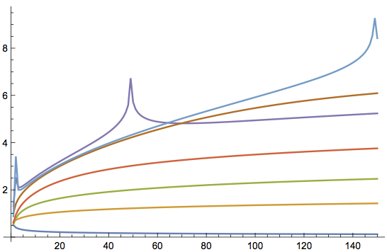
Figure 1: Plot giving the accuracy of the double-scaled estimates of the MMP function through N⁶LO, plotted as the number of digits of accuracy of each of the estimates, as a function of $n$. The quantity being plotted is $-{1\over{{\rm Log}[10]}}$ the logarithm of the relative error in the estimate of the MMP function. The horizontal axis is $n$, and the vertical axis is $-{1\over{{\rm Log}[10]}}\,{\rm Log}\left|\,{{q_{n}^{({\rm{\textsc{mmp}}})}-(q_{n}^{({\rm{\textsc{mmp}}})})_{{\rm{estimate}}}}\over{q_{n}^{({\rm{\textsc{mmp}}})}}}\,\right|$. The LO, NLO, N²LO, N³LO, N⁴LO, N⁵LO and N⁶LO estimates are given by the blue, yellow, green, red, and purple, brown, and light blue curves respectively, which are in ascending order on the chart for $n\gtrsim 65$. The upward spikes on the accuracy plots of the N⁴LO and N⁶LO estimates are ”accidental accuracies” in which the estimate transitions between slightly overestimating and slightly underestimating the exact result as $n$ is varied, generating an atypically precise estimate at N⁴LO and N⁶LO in certain limited ranges of $n$. At $n=150$ the N⁵LO fixed-$\tau$ large-$n$ estimate of the MMP function is accurate to one part in $10^{6}$ and the N⁶LO fixed-$\tau$ large-$n$ estimate is accurate to one part in $10^{8}$.

4.3.3 Plotting the log of relative error of the fixed-$\tau$ estimates through order $n^{-{5\over 2}}$ in the exponent, evaluated at $\tau={{25}\over\pi},1\leq n\leq 150.$, relative to the full log of the scheme-independent correlator
$\tilde{G}_{2n}\equiv{{G_{2n}}\over{(G_{2})^{n}}}=e^{q_{n}-n\,q_{1}+(n-1)q_{0}}$

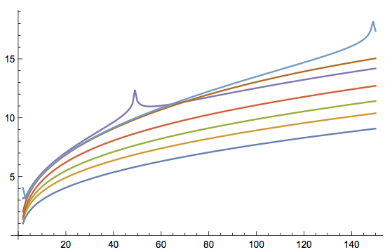
Figure 2: Plot giving the accuracy of the fixed-coupling large-R-charge estimates of the full log of the scheme-independent correlator, $\tilde{q}_{n}\equiv{\rm Log}[\tilde{G}_{2n}]\equiv q_{n}-n\,q_{1}+(n-1)q_{0}$. The estimate for $\tilde{q}_{n}$ is defined to be $(\tilde{q}_{n})_{{\rm{estimate}}}\equiv(q_{n}^{({\rm{\textsc{mmp}}})})_{{\rm{estimate}}}+q_{n}^{({\rm{eft}})}-nq_{1}+(n-1)q_{0}$, with the MMP contribution as estimated by eqs. (3.13),(3.15),(3.106)-(3.114) through N⁶LO. The quantity being plotted is $-{1\over{{\rm Log}[10]}}$ times the logarithm of the relative error in the estimate of the correlator. The horizontal axis is $n$, and the vertical axis is $y(n)\equiv-{1\over{{\rm Log}[10]}}\,{\rm Log}\left|\,{{{\rm Log}[\tilde{G}_{2n}^{{\rm{exact}}}]-{\rm Log}[\tilde{G}_{2n}^{{\rm{estimate}}}]}\over{{\rm Log}[\tilde{G}_{2n}^{{\rm{exact}}}]}}\,\right|=-{1\over{{\rm Log}[10]}}\,{\rm Log}\left|\,{{q_{n}^{({\rm{\textsc{mmp}}})}-(q_{n}^{({\rm{\textsc{mmp}}})})_{{\rm{estimate}}}}\over{q_{n}-n\,q_{1}+(n-1)q_{0}}}\,\right|$. The leading-order, NLO, N²LO, N³LO, N⁴LO, N⁵LO and N⁶LO estimates are given by the dark blue, yellow, green, red, and purple, brown, and light blue curves respectively. The upward spikes on the accuracy of the N⁴LO and N⁶LO estimates are ”accidental accuracies” in which an estimate transitions between slightly overestimating and slightly underestimating the exact result as $n$ is varied, generating an atypically precise estimate in some limited range of $n$. At $n=150$ the N⁵LO fixed-$\tau$ large-$n$ estimate of the scheme-independent correlator is accurate to one part in $10^{15}$ and the N⁶LO estimate is accurate to one part in $10^{17}$.

4.4 Table of values of the fixed-$\tau$ large-charge asymptotic estimates at $\tau={{25}\over\pi}\,i$, up to $n=150$

	${{e^{-S_{{\rm{WLI}}}}{\rm~{}w}/}\atop{\rm prefactor}}$	${{\rm estimate~{}w/}\atop{O(n^{-{1\over 2}})}}$	${{\rm estimate~{}w/}\atop{O(n^{-1})}}$	${{\rm estimate~{}w/}\atop{O(n^{-{3\over 2}})}}$	${{\rm estimate~{}w/}\atop{O(n^{-2})}}$	${{\rm estimate~{}w/}\atop{O(n^{-{5\over 2}})}}$	${{\rm exact}\atop{q_{n}^{({\rm{\textsc{mmp}}})}}}$
1	0.3306547971	0.5494056108	0.3208548662	0.4473688062	0.3855992091	0.4826779760	0.4263073863
2	0.2369155213	0.3392528251	0.2592574487	0.2915876823	0.2809550113	0.2923319506	0.2924432054
3	0.1777356756	0.2382818085	0.1991725121	0.2123297908	0.2088531261	0.2118834217	0.2140116919
4	0.1376160664	0.1773896477	0.1550715601	0.1616504023	0.1601561764	0.1612839808	0.1629019007
5	0.1090165541	0.1368079122	0.1228554207	0.1265627818	0.1258128005	0.1263191935	0.1274138410
6	0.08788478715	0.1081284329	0.09885739579	0.1011186866	0.1007021939	0.1009589550	0.1016922546
7	0.07184428016	0.08704428588	0.08060668448	0.08206644241	0.08181796572	0.08195980455	0.08245642599
8	0.05940855833	0.07109089681	0.06646850876	0.06745213130	0.06729571354	0.06737924445	0.06772080050
9	0.04960141702	0.05874895841	0.05534091587	0.05602642358	0.05592374401	0.05597544585	0.05621405675
10	0.04175689585	0.04903003507	0.04646262665	0.04695358198	0.04688386790	0.04691717164	0.04708632558
11	0.03540658081	0.04126413514	0.03929504552	0.03965469749	0.03960603245	0.03962819994	0.03974973039
12	0.03021262008	0.03498215250	0.03344884738	0.03371738216	0.03368260919	0.03369777501	0.03378615497
13	0.02592614410	0.02984686301	0.02863720688	0.02884100969	0.02881566382	0.02882628483	0.02889126648
14	0.02236051076	0.02561047918	0.02464524274	0.02480212485	0.02478332983	0.02479091948	0.02483917594
15	0.01937356121	0.02208752376	0.02130957226	0.02143184640	0.02141769798	0.02142321768	0.02145938050
16	0.01685554371	0.01913693280	0.01850432737	0.01860068261	0.01858988973	0.01859396672	0.01862129258
17	0.01472070962	0.01664992496	0.01613139844	0.01620807852	0.01619974753	0.01620280064	0.01622360696
18	0.01290134962	0.01454158672	0.01411350505	0.01417506884	0.01416856972	0.01417088442	0.01418683837
19	0.01134348831	0.01274491628	0.01238919441	0.01243901837	0.01243389962	0.01243567409	0.01244798710
20	0.01000372820	0.01120653279	0.01090917838	0.01094979540	0.01094572872	0.01094710280	0.01095666332
21	0.008846904394	0.009883536354	0.009633615187	0.009666947415	0.009663690908	0.009664764735	0.009672229925
22	0.007844320098	0.008741177896	0.008530067806	0.008557589292	0.008554962571	0.008555808820	0.008561668609
23	0.006972404298	0.007751108180	0.007571953743	0.007594805756	0.007592672836	0.007593344899	0.007597967228
24	0.006211680108	0.006890046993	0.006737356034	0.006756429974	0.006754687312	0.006755224851	0.006758887946
25	0.005545964521	0.006138761199	0.006008102884	0.006024100625	0.006022668651	0.006023101434	0.006026017027
26	0.004961742339	0.005481272548	0.005369049148	0.005382527465	0.005381344515	0.005381695095	0.005384025281
27	0.004447672504	0.004904238255	0.004807510976	0.004818914601	0.004817932510	0.004818218124	0.004820087697
28	0.003994195976	0.004396462814	0.004312817709	0.004322504168	0.004321685038	0.004321918968	0.004323424514
29	0.003593222175	0.003948510385	0.003875954302	0.003884212735	0.003883526547	0.003883719104	0.003884935751
30	0.003237876660	0.003552394945	0.003489274164	0.003496339719	0.003495762541	0.003495921786	0.003496908245

Table 1: The successive refined estimates for the massive macroscopic propagation function $q_{n}^{({\rm{\textsc{mmp}}})}\equiv q_{n}-q_{n}^{({\rm{eft}})}$, at the coupling $\tau={{25i}\over{\pi}}$. The first column, ”$e^{-S_{{\rm{WLI}}}}$ with prefactor” is the approximation $q_{n}^{({\rm{\textsc{mmp}}})}\simeq\big{[}\,{{2^{13}\,n}\over{\pi^{5}\,{\rm Im}[\sigma]}}\,\big{]}^{+{1\over 4}}\,{\rm exp}\{-\sqrt{{8\pi n}\over{{\rm Im}[\sigma]}}\}$, with $\sigma$ denoting the infrared coupling related to the UV coupling $\tau$ by $e^{2\pi i\tau}=\lambda[\sigma],$ where $\lambda[\sigma]$ is the modular lambda function. The value of $\tau$ in this table is $\tau={{25}\over\pi}\,i$. In each successive column we add a correction of the form $-n^{-{p\over 2}}\,w_{p}[\sigma]$ to the exponent of the exponential for $p=1,\cdots 5$. The functions $w_{p}[\sigma]$ are given explictly in eqs. (3.106)-(3.114)

.

	${{e^{-S_{{\rm{WLI}}}}{\rm~{}w}/}\atop{\rm prefactor}}$	${{\rm estimate~{}w/}\atop{O(n^{-{1\over 2}})}}$	${{\rm estimate~{}w/}\atop{O(n^{-1})}}$	${{\rm estimate~{}w/}\atop{O(n^{-{3\over 2}})}}$	${{\rm estimate~{}w/}\atop{O(n^{-2})}}$	${{\rm estimate~{}w/}\atop{O(n^{-{5\over 2}})}}$	${{\rm exact}\atop{q_{n}^{({\rm{\textsc{mmp}}})}}}$
31	0.002922296878	0.003201331023	0.003146267184	0.003152332104	0.003151844745	0.003151977022	0.003152779381
32	0.002641465936	0.002889531972	0.002841371302	0.002846593527	0.002846180510	0.002846290844	0.002846945436
33	0.002391076604	0.002612045828	0.002569818642	0.002574328534	0.002573977313	0.002574069707	0.002574605288
34	0.002167419511	0.002364621035	0.002327509260	0.002331414888	0.002331115242	0.002331192901	0.002331632319
35	0.001967290819	0.002143596083	0.002110907063	0.002114298388	0.002114041953	0.002114107457	0.002114468932
36	0.001787915643	0.001945808373	0.001916953643	0.001919905844	0.001919685741	0.001919741178	0.001920039289
37	0.001626884277	0.001768518637	0.001742996630	0.001745572764	0.001745383318	0.001745430384	0.001745676837
38	0.001482098879	0.001609348000	0.001586729899	0.001588983046	0.001588819551	0.001588859632	0.001589063854
39	0.001351728735	0.001466225365	0.001446143478	0.001448118466	0.001447977008	0.001448011239	0.001448180848
40	0.001234172590	0.001337343268	0.001319481435	0.001321216247	0.001321093558	0.001321122874	0.001321264040
41	0.001128026830	0.001221120707	0.001205206358	0.001206733271	0.001206626612	0.001206651784	0.001206769522
42	0.001032058507	0.001116171746	0.001101969286	0.001103315811	0.001103222881	0.001103244551	0.001103342946
43	0.0009451824252	0.001021278896	0.001008584201	0.001009773851	0.001009692709	0.001009711409	0.001009793798
44	0.0008664415919	0.0009353705035	0.0009240063010	0.0009250592249	0.0009249882309	0.0009250044051	0.0009250735212
45	0.0007949905180	0.0008575014645	0.0008473134585	0.0008482469668	0.0008481847288	0.0008481987498	0.0008482568358
46	0.0007300809000	0.0007868367408	0.0007776903459	0.0007785193470	0.0007784646815	0.0007784768620	0.0007785257633
47	0.0006710493189	0.0007226372331	0.0007144148153	0.0007151521785	0.0007151040766	0.0007151146799	0.0007151559185
48	0.0006173066448	0.0006642476420	0.0006568461799	0.0006575030396	0.0006574606387	0.0006574698874	0.0006575047208
49	0.0005683288901	0.0006110860113	0.0006044151093	0.0006050011198	0.0006049636807	0.0006049717634	0.0006050012329
50	0.0005236492943	0.0005626347012	0.0005566148966	0.0005571384461	0.0005571053342	0.0005571124109	0.0005571373807
51	0.0004828514617	0.0005184325769	0.0005129938943	0.0005134622857	0.0005134329544	0.0005134391614	0.0005134603500
52	0.0004455633979	0.0004780682350	0.0004731489485	0.0004735685520	0.0004735425302	0.0004735479836	0.0004735659895
53	0.0004114523178	0.0004411741180	0.0004367196891	0.0004370960719	0.0004370729519	0.0004370777512	0.0004370930739
54	0.0003802201166	0.0004074213892	0.0004033835532	0.0004037215894	0.0004037010183	0.0004037052488	0.0004037183057
55	0.0003515994118	0.0003765154626	0.0003728514412	0.0003731554055	0.0003731370769	0.0003731408118	0.0003731519527
56	0.0003253500775	0.0003481920948	0.0003448639164	0.0003451375640	0.0003451212116	0.0003451245140	0.0003451340321
57	0.0003012562054	0.0003222139647	0.0003191878753	0.0003194345108	0.0003194199026	0.0003194228267	0.0003194309685
58	0.0002791234344	0.0002983676725	0.0002956136258	0.0002958361615	0.0002958230949	0.0002958256878	0.0002958326607
59	0.0002587766014	0.0002764611036	0.0002739523175	0.0002741533239	0.0002741416221	0.0002741439244	0.0002741499032
60	0.0002400576708	0.0002563211089	0.0002540336796	0.0002542154292	0.0002542049370	0.0002542069841	0.0002542121164

Table 2: The successive refined estimates for the massive macroscopic propagation function $q_{n}^{({\rm{\textsc{mmp}}})}\equiv q_{n}-q_{n}^{({\rm{eft}})}$, at the coupling $\tau={{25i}\over{\pi}}$. The first column, ”$e^{-S_{{\rm{WLI}}}}$ with prefactor” is the approximation $q_{n}^{({\rm{\textsc{mmp}}})}\simeq\big{[}\,{{2^{13}\,n}\over{\pi^{5}\,{\rm Im}[\sigma]}}\,\big{]}^{+{1\over 4}}\,{\rm exp}\{-\sqrt{{8\pi n}\over{{\rm Im}[\sigma]}}\}$, with $\sigma$ denoting the infrared coupling related to the UV coupling $\tau$ by $e^{2\pi i\tau}=\lambda[\sigma],$ where $\lambda[\sigma]$ is the modular lambda function. The value of $\tau$ in this table is $\tau={{25}\over\pi}\,i$. In each successive column we add a correction of the form $-n^{-{p\over 2}}\,w_{p}[\sigma]$ to the exponent of the exponential for $p=1,\cdots 5$. The functions $w_{p}[\sigma]$ are given explictly in eqs. (3.106)-(3.114)

.

	${{e^{-S_{{\rm{WLI}}}}{\rm~{}w}/}\atop{\rm prefactor}}$	${{\rm estimate~{}w/}\atop{O(n^{-{1\over 2}})}}$	${{\rm estimate~{}w/}\atop{O(n^{-1})}}$	${{\rm estimate~{}w/}\atop{O(n^{-{3\over 2}})}}$	${{\rm estimate~{}w/}\atop{O(n^{-2})}}$	${{\rm estimate~{}w/}\atop{O(n^{-{5\over 2}})}}$	${{\rm exact}\atop{q_{n}^{({\rm{\textsc{mmp}}})}}}$
61	0.0002228239063	0.0002377914602	0.0002357040259	0.0002358685302	0.0002358591119	0.0002358609343	0.0002358653448
62	0.0002069462559	0.0002207310457	0.0002188244923	0.0002189735347	0.0002189650708	0.0002189666952	0.0002189704896
63	0.0001923079213	0.0002050122741	0.0002032694786	0.0002034046422	0.0002033970276	0.0002033984774	0.0002034017450
64	0.0001788030905	0.0001905196626	0.0001889252678	0.0001890479594	0.0001890411017	0.0001890423972	0.0001890452141
65	0.0001663358121	0.0001771485847	0.0001756888014	0.0001758002733	0.0001757940909	0.0001757952498	0.0001757976806
66	0.0001548189954	0.0001648041588	0.0001634665919	0.0001635679601	0.0001635623808	0.0001635634187	0.0001635655183
67	0.0001441735199	0.0001534002598	0.0001521737559	0.0001522660158	0.0001522609759	0.0001522619064	0.0001522637217
68	0.0001343274424	0.0001428586406	0.0001417331527	0.0001418171936	0.0001418126366	0.0001418134717	0.0001418150425
69	0.0001252152894	0.0001331081479	0.0001320746166	0.0001321512336	0.0001321471094	0.0001321478597	0.0001321492202
70	0.0001167774246	0.0001240840233	0.0001231342717	0.0001232041768	0.0001232004409	0.0001232011157	0.0001232022950
71	0.0001089594845	0.0001157272792	0.0001148539196	0.0001149177508	0.0001149143636	0.0001149149711	0.0001149159943
72	0.0001017118719	0.0001079841400	0.0001071804917	0.0001072388213	0.0001072357476	0.0001072362950	0.0001072371835
73	0.00009498930276	0.0001008055423	0.0001000655584	0.0001001189005	0.0001001161089	0.0001001166027	0.0001001173747
74	0.00008875039937	0.00009414668731	0.00009346488944	0.00009351370610	0.00009351116875	0.00009351161451	0.00009351228591
75	0.00008295732519	0.00008796663846	0.00008733805916	0.00008738276627	0.00008738045807	0.00008738086086	0.00008738144519
76	0.00007757545647	0.00008222796063	0.00008164809185	0.00008168906396	0.00008168696257	0.00008168732685	0.00008168783576
77	0.00007257308678	0.00007689639567	0.00007636114281	0.00007639871763	0.00007639680305	0.00007639713279	0.00007639757633
78	0.00006792116092	0.00007194057038	0.00007144621139	0.00007148069366	0.00007147894796	0.00007147924668	0.00007147963351
79	0.00006359303508	0.00006733173349	0.00006687488227	0.00006690654723	0.00006690495434	0.00006690522518	0.00006690556278
80	0.00005956426027	0.00006304351857	0.00006262109222	0.00006265018869	0.00006264873419	0.00006264897995	0.00006264927477
81	0.00005581238694	0.00005905173003	0.00005866091959	0.00005868767269	0.00005868634362	0.00005868656680	0.00005868682442
82	0.00005231678815	0.00005533414987	0.00005497239407	0.00005499700765	0.00005499579236	0.00005499599518	0.00005499622043
83	0.00004905849977	0.00005187036297	0.00005153532468	0.00005155798349	0.00005155687147	0.00005155705594	0.00005155725300
84	0.00004602007569	0.00004864159906	0.00004833114414	0.00004835201573	0.00004835099755	0.00004835116544	0.00004835133795
85	0.00004318545662	0.00004563058954	0.00004534276787	0.00004536200435	0.00004536107147	0.00004536122438	0.00004536137547
86	0.00004053985115	0.00004282143782	0.00004255446620	0.00004257220572	0.00004257135045	0.00004257148983	0.00004257162223
87	0.00003806962771	0.00004019950164	0.00003995174843	0.00003996811658	0.00003996733198	0.00003996745910	0.00003996757518
88	0.00003576221656	0.00003775128635	0.00003752125755	0.00003753636860	0.00003753564839	0.00003753576442	0.00003753586624
89	0.00003360602056	0.00003546434784	0.00003525067466	0.00003526463263	0.00003526397113	0.00003526407710	0.00003526416645
90	0.00003159033412	0.00003332720441	0.00003312863197	0.00003314153162	0.00003314092369	0.00003314102053	0.00003314109898

Table 3: The successive refined estimates for the massive macroscopic propagation function $q_{n}^{({\rm{\textsc{mmp}}})}\equiv q_{n}-q_{n}^{({\rm{eft}})}$, at the coupling $\tau={{25i}\over{\pi}}$. The first column, ”$e^{-S_{{\rm{WLI}}}}$ with prefactor” is the approximation $q_{n}^{({\rm{\textsc{mmp}}})}\simeq\big{[}\,{{2^{13}\,n}\over{\pi^{5}\,{\rm Im}[\sigma]}}\,\big{]}^{+{1\over 4}}\,{\rm exp}\{-\sqrt{{8\pi n}\over{{\rm Im}[\sigma]}}\}$, with $\sigma$ denoting the infrared coupling related to the UV coupling $\tau$ by $e^{2\pi i\tau}=\lambda[\sigma],$ where $\lambda[\sigma]$ is the modular lambda function. The value of $\tau$ in this table is $\tau={{25}\over\pi}\,i$. In each successive column we add a correction of the form $-n^{-{p\over 2}}\,w_{p}[\sigma]$ to the exponent of the exponential for $p=1,\cdots 5$. The functions $w_{p}[\sigma]$ are given explictly in eqs. (3.106)-(3.114)

.

	${{e^{-S_{{\rm{WLI}}}}{\rm~{}w}/}\atop{\rm prefactor}}$	${{\rm estimate~{}w/}\atop{O(n^{-{1\over 2}})}}$	${{\rm estimate~{}w/}\atop{O(n^{-1})}}$	${{\rm estimate~{}w/}\atop{O(n^{-{3\over 2}})}}$	${{\rm estimate~{}w/}\atop{O(n^{-2})}}$	${{\rm estimate~{}w/}\atop{O(n^{-{5\over 2}})}}$	${{\rm exact}\atop{q_{n}^{({\rm{\textsc{mmp}}})}}}$
91	0.00002970526931	0.00003132925656	0.00003114463367	0.00003115656141	0.00003115600238	0.00003115609094	0.00003115615984
92	0.00002794168866	0.00002946071395	0.00002928898394	0.00002930001857	0.00002929950422	0.00002929958526	0.00002929964580
93	0.00002629114378	0.00002771252889	0.00002755272122	0.00002756293471	0.00002756246120	0.00002756253540	0.00002756258862
94	0.00002474581949	0.00002607633566	0.00002592755843	0.00002593701650	0.00002593658035	0.00002593664834	0.00002593669514
95	0.00002329848272	0.00002454439522	0.00002440582830	0.00002441459104	0.00002441418909	0.00002441425141	0.00002441429258
96	0.00002194243589	0.00002310954469	0.00002298043354	0.00002298855589	0.00002298818526	0.00002298824243	0.00002298827865
97	0.00002067147429	0.00002176515122	0.00002164480122	0.00002165233348	0.00002165199155	0.00002165204402	0.00002165207590
98	0.00001947984709	0.00002050506980	0.00002039284119	0.00002039982941	0.00002039951380	0.00002039956198	0.00002039959005
99	0.00001836222166	0.00001932360471	0.00001921890791	0.00001922539430	0.00001922510284	0.00001922514711	0.00001922517183
100	0.00001731365088	0.00001821547422	0.00001811776564	0.00001812378889	0.00001812351960	0.00001812356029	0.00001812358207
101	0.00001632954327	0.00001717577827	0.00001708455643	0.00001709015203	0.00001708990310	0.00001708994053	0.00001708995971
102	0.00001540563547	0.00001619996883	0.00001611477088	0.00001611997141	0.00001611974120	0.00001611977565	0.00001611979255
103	0.00001453796714	0.00001528382277	0.00001520422131	0.00001520905670	0.00001520884369	0.00001520887541	0.00001520889031
104	0.00001372285780	0.00001442341693	0.00001434901710	0.00001435351484	0.00001435331766	0.00001435334688	0.00001435336001
105	0.00001295688564	0.00001361510529	0.00001354554210	0.00001354972747	0.00001354954486	0.00001354957179	0.00001354958336
106	0.00001223686802	0.00001285549794	0.00001279043386	0.00001279433010	0.00001279416091	0.00001279418575	0.00001279419595
107	0.00001155984356	0.00001214144179	0.00001208056453	0.00001208419306	0.00001208403624	0.00001208405915	0.00001208406814
108	0.00001092305564	0.00001147000284	0.00001141302337	0.00001141640388	0.00001141625845	0.00001141627960	0.00001141628753
109	0.00001032393722	0.00001083844988	0.00001078510051	0.00001078825118	0.00001078811626	0.00001078813579	0.00001078814278
110	9.760096897$\times 10^{-6}$	0.00001024423944	0.00001019427220	0.00001019720974	0.00001019708452	0.00001019710256	0.00001019710872
111	9.229306029$\times 10^{-6}$	9.685001983$\times 10^{-6}$	9.638187027$\times 10^{-6}$	9.640926874$\times 10^{-6}$	9.640810611$\times 10^{-6}$	9.640827288$\times 10^{-6}$	9.640832718$\times 10^{-6}$
112	8.729486868$\times 10^{-6}$	9.158529175$\times 10^{-6}$	9.114653382$\times 10^{-6}$	9.117209776$\times 10^{-6}$	9.117101782$\times 10^{-6}$	9.117117204$\times 10^{-6}$	9.117121989$\times 10^{-6}$
113	8.258701627$\times 10^{-6}$	8.662762128$\times 10^{-6}$	8.621627798$\times 10^{-6}$	8.624013880$\times 10^{-6}$	8.623913529$\times 10^{-6}$	8.623927795$\times 10^{-6}$	8.623932012$\times 10^{-6}$
114	7.815142395$\times 10^{-6}$	8.195780584$\times 10^{-6}$	8.157204245$\times 10^{-6}$	8.159432152$\times 10^{-6}$	8.159338865$\times 10^{-6}$	8.159352069$\times 10^{-6}$	8.159355782$\times 10^{-6}$
115	7.397121821$\times 10^{-6}$	7.755792923$\times 10^{-6}$	7.719604237$\times 10^{-6}$	7.721685182$\times 10^{-6}$	7.721598428$\times 10^{-6}$	7.721610654$\times 10^{-6}$	7.721613924$\times 10^{-6}$
116	7.003064516$\times 10^{-6}$	7.341126943$\times 10^{-6}$	7.307167705$\times 10^{-6}$	7.309112051$\times 10^{-6}$	7.309031343$\times 10^{-6}$	7.309042667$\times 10^{-6}$	7.309045546$\times 10^{-6}$
117	6.631499111$\times 10^{-6}$	6.950221352$\times 10^{-6}$	6.918344563$\times 10^{-6}$	6.920161895$\times 10^{-6}$	6.920086781$\times 10^{-6}$	6.920097276$\times 10^{-6}$	6.920099809$\times 10^{-6}$
118	6.281050911$\times 10^{-6}$	6.581617895$\times 10^{-6}$	6.551686917$\times 10^{-6}$	6.553386101$\times 10^{-6}$	6.553316169$\times 10^{-6}$	6.553325898$\times 10^{-6}$	6.553328125$\times 10^{-6}$
119	5.950435111$\times 10^{-6}$	6.233954090$\times 10^{-6}$	6.205841867$\times 10^{-6}$	6.207431107$\times 10^{-6}$	6.207365976$\times 10^{-6}$	6.207374999$\times 10^{-6}$	6.207376957$\times 10^{-6}$
120	5.638450512$\times 10^{-6}$	5.905956503$\times 10^{-6}$	5.879544842$\times 10^{-6}$	5.881031737$\times 10^{-6}$	5.880971055$\times 10^{-6}$	5.880979426$\times 10^{-6}$	5.880981146$\times 10^{-6}$

Table 4: The successive refined estimates for the massive macroscopic propagation function $q_{n}^{({\rm{\textsc{mmp}}})}\equiv q_{n}-q_{n}^{({\rm{eft}})}$, at the coupling $\tau={{25i}\over{\pi}}$. The first column, ”$e^{-S_{{\rm{WLI}}}}$ with prefactor” is the approximation $q_{n}^{({\rm{\textsc{mmp}}})}\simeq\big{[}\,{{2^{13}\,n}\over{\pi^{5}\,{\rm Im}[\sigma]}}\,\big{]}^{+{1\over 4}}\,{\rm exp}\{-\sqrt{{8\pi n}\over{{\rm Im}[\sigma]}}\}$, with $\sigma$ denoting the infrared coupling related to the UV coupling $\tau$ by $e^{2\pi i\tau}=\lambda[\sigma],$ where $\lambda[\sigma]$ is the modular lambda function. The value of $\tau$ in this table is $\tau={{25}\over\pi}\,i$. In each successive column we add a correction of the form $-n^{-{p\over 2}}\,w_{p}[\sigma]$ to the exponent of the exponential for $p=1,\cdots 5$. The functions $w_{p}[\sigma]$ are given explictly in eqs. (3.106)-(3.114)

.

	${{e^{-S_{{\rm{WLI}}}}{\rm~{}w}/}\atop{\rm prefactor}}$	${{\rm estimate~{}w/}\atop{O(n^{-{1\over 2}})}}$	${{\rm estimate~{}w/}\atop{O(n^{-1})}}$	${{\rm estimate~{}w/}\atop{O(n^{-{3\over 2}})}}$	${{\rm estimate~{}w/}\atop{O(n^{-2})}}$	${{\rm estimate~{}w/}\atop{O(n^{-{5\over 2}})}}$	${{\rm exact}\atop{q_{n}^{({\rm{\textsc{mmp}}})}}}$
121	5.343973708$\times 10^{-6}$	5.596434531$\times 10^{-6}$	5.571613442$\times 10^{-6}$	5.573005031$\times 10^{-6}$	5.572948473$\times 10^{-6}$	5.572956243$\times 10^{-6}$	5.572957753$\times 10^{-6}$
122	5.065953711$\times 10^{-6}$	5.304274642$\times 10^{-6}$	5.280941735$\times 10^{-6}$	5.282244539$\times 10^{-6}$	5.282191807$\times 10^{-6}$	5.282199022$\times 10^{-6}$	5.282200346$\times 10^{-6}$
123	4.803406960$\times 10^{-6}$	5.028435053$\times 10^{-6}$	5.006494974$\times 10^{-6}$	5.007715039$\times 10^{-6}$	5.007665857$\times 10^{-6}$	5.007672559$\times 10^{-6}$	5.007673719$\times 10^{-6}$
124	4.555412707$\times 10^{-6}$	4.767940789$\times 10^{-6}$	4.747304706$\times 10^{-6}$	4.748447639$\times 10^{-6}$	4.748401753$\times 10^{-6}$	4.748407980$\times 10^{-6}$	4.748408996$\times 10^{-6}$
125	4.321108734$\times 10^{-6}$	4.521879112$\times 10^{-6}$	4.502464239$\times 10^{-6}$	4.503535242$\times 10^{-6}$	4.503492416$\times 10^{-6}$	4.503498205$\times 10^{-6}$	4.503499093$\times 10^{-6}$
126	4.099687382$\times 10^{-6}$	4.289395279$\times 10^{-6}$	4.271124437$\times 10^{-6}$	4.272128338$\times 10^{-6}$	4.272088355$\times 10^{-6}$	4.272093738$\times 10^{-6}$	4.272094514$\times 10^{-6}$
127	3.890391871$\times 10^{-6}$	4.069688609$\times 10^{-6}$	4.052489823$\times 10^{-6}$	4.053431107$\times 10^{-6}$	4.053393766$\times 10^{-6}$	4.053398773$\times 10^{-6}$	4.053399450$\times 10^{-6}$
128	3.692512878$\times 10^{-6}$	3.862008840$\times 10^{-6}$	3.845814964$\times 10^{-6}$	3.846697794$\times 10^{-6}$	3.846662909$\times 10^{-6}$	3.846667569$\times 10^{-6}$	3.846668157$\times 10^{-6}$
129	3.505385368$\times 10^{-6}$	3.665652736$\times 10^{-6}$	3.650401109$\times 10^{-6}$	3.651229354$\times 10^{-6}$	3.651196753$\times 10^{-6}$	3.651201091$\times 10^{-6}$	3.651201602$\times 10^{-6}$
130	3.328385640$\times 10^{-6}$	3.479960950$\times 10^{-6}$	3.465593075$\times 10^{-6}$	3.466370332$\times 10^{-6}$	3.466339856$\times 10^{-6}$	3.466343896$\times 10^{-6}$	3.466344339$\times 10^{-6}$
131	3.160928593$\times 10^{-6}$	3.304315100$\times 10^{-6}$	3.290776351$\times 10^{-6}$	3.291505965$\times 10^{-6}$	3.291477466$\times 10^{-6}$	3.291481229$\times 10^{-6}$	3.291481613$\times 10^{-6}$
132	3.002465179$\times 10^{-6}$	3.138135057$\times 10^{-6}$	3.125374406$\times 10^{-6}$	3.126059487$\times 10^{-6}$	3.126032830$\times 10^{-6}$	3.126036336$\times 10^{-6}$	3.126036667$\times 10^{-6}$
133	2.852480037$\times 10^{-6}$	2.980876423$\times 10^{-6}$	2.968846188$\times 10^{-6}$	2.969489632$\times 10^{-6}$	2.969464689$\times 10^{-6}$	2.969467958$\times 10^{-6}$	2.969468243$\times 10^{-6}$
134	2.710489289$\times 10^{-6}$	2.832028189$\times 10^{-6}$	2.820683800$\times 10^{-6}$	2.821288301$\times 10^{-6}$	2.821264956$\times 10^{-6}$	2.821268003$\times 10^{-6}$	2.821268247$\times 10^{-6}$
135	2.576038494$\times 10^{-6}$	2.691110548$\times 10^{-6}$	2.680410332$\times 10^{-6}$	2.680978400$\times 10^{-6}$	2.680956543$\times 10^{-6}$	2.680959386$\times 10^{-6}$	2.680959594$\times 10^{-6}$
136	2.448700739$\times 10^{-6}$	2.557672873$\times 10^{-6}$	2.547577851$\times 10^{-6}$	2.548111823$\times 10^{-6}$	2.548091353$\times 10^{-6}$	2.548094006$\times 10^{-6}$	2.548094183$\times 10^{-6}$
137	2.328074866$\times 10^{-6}$	2.431291819$\times 10^{-6}$	2.421765526$\times 10^{-6}$	2.422267580$\times 10^{-6}$	2.422248404$\times 10^{-6}$	2.422250880$\times 10^{-6}$	2.422251029$\times 10^{-6}$
138	2.213783817$\times 10^{-6}$	2.311569574$\times 10^{-6}$	2.302577881$\times 10^{-6}$	2.303050047$\times 10^{-6}$	2.303032078$\times 10^{-6}$	2.303034389$\times 10^{-6}$	2.303034515$\times 10^{-6}$
139	2.105473094$\times 10^{-6}$	2.198132213$\times 10^{-6}$	2.189643171$\times 10^{-6}$	2.190087340$\times 10^{-6}$	2.190070498$\times 10^{-6}$	2.190072657$\times 10^{-6}$	2.190072761$\times 10^{-6}$
140	2.002809320$\times 10^{-6}$	2.090628173$\times 10^{-6}$	2.082611864$\times 10^{-6}$	2.083029804$\times 10^{-6}$	2.083014012$\times 10^{-6}$	2.083016029$\times 10^{-6}$	2.083016115$\times 10^{-6}$
141	1.905478906$\times 10^{-6}$	1.988726831$\times 10^{-6}$	1.981155232$\times 10^{-6}$	1.981548589$\times 10^{-6}$	1.981533780$\times 10^{-6}$	1.981535665$\times 10^{-6}$	1.981535734$\times 10^{-6}$
142	1.813186795$\times 10^{-6}$	1.892117180$\times 10^{-6}$	1.884964034$\times 10^{-6}$	1.885334345$\times 10^{-6}$	1.885320452$\times 10^{-6}$	1.885322214$\times 10^{-6}$	1.885322270$\times 10^{-6}$
143	1.725655303$\times 10^{-6}$	1.800506585$\times 10^{-6}$	1.793747283$\times 10^{-6}$	1.794095984$\times 10^{-6}$	1.794082948$\times 10^{-6}$	1.794084595$\times 10^{-6}$	1.794084639$\times 10^{-6}$
144	1.642623030$\times 10^{-6}$	1.713619633$\times 10^{-6}$	1.707231106$\times 10^{-6}$	1.707559537$\times 10^{-6}$	1.707547301$\times 10^{-6}$	1.707548842$\times 10^{-6}$	1.707548876$\times 10^{-6}$
145	1.563843842$\times 10^{-6}$	1.631197057$\times 10^{-6}$	1.625157670$\times 10^{-6}$	1.625467083$\times 10^{-6}$	1.625455596$\times 10^{-6}$	1.625457038$\times 10^{-6}$	1.625457062$\times 10^{-6}$
146	1.489085927$\times 10^{-6}$	1.552994725$\times 10^{-6}$	1.547284187$\times 10^{-6}$	1.547575752$\times 10^{-6}$	1.547564964$\times 10^{-6}$	1.547566314$\times 10^{-6}$	1.547566330$\times 10^{-6}$
147	1.418130909$\times 10^{-6}$	1.478782705$\times 10^{-6}$	1.473381976$\times 10^{-6}$	1.473656786$\times 10^{-6}$	1.473646653$\times 10^{-6}$	1.473647916$\times 10^{-6}$	1.473647926$\times 10^{-6}$
148	1.350773019$\times 10^{-6}$	1.408344385$\times 10^{-6}$	1.403235597$\times 10^{-6}$	1.403494676$\times 10^{-6}$	1.403485155$\times 10^{-6}$	1.403486338$\times 10^{-6}$	1.403486342$\times 10^{-6}$
149	1.286818322$\times 10^{-6}$	1.341475655$\times 10^{-6}$	1.336642035$\times 10^{-6}$	1.336886338$\times 10^{-6}$	1.336877391$\times 10^{-6}$	1.336878498$\times 10^{-6}$	1.336878498$\times 10^{-6}$
150	1.226083996$\times 10^{-6}$	1.277984141$\times 10^{-6}$	1.273409938$\times 10^{-6}$	1.273640360$\times 10^{-6}$	1.273631949$\times 10^{-6}$	1.273632987$\times 10^{-6}$	1.273632982$\times 10^{-6}$

Table 5: The successive refined estimates for the massive macroscopic propagation function $q_{n}^{({\rm{\textsc{mmp}}})}\equiv q_{n}-q_{n}^{({\rm{eft}})}$, at the coupling $\tau={{25i}\over{\pi}}$. The first column, ”$e^{-S_{{\rm{WLI}}}}$ with prefactor” is the approximation $q_{n}^{({\rm{\textsc{mmp}}})}\simeq\big{[}\,{{2^{13}\,n}\over{\pi^{5}\,{\rm Im}[\sigma]}}\,\big{]}^{+{1\over 4}}\,{\rm exp}\{-\sqrt{{8\pi n}\over{{\rm Im}[\sigma]}}\}$, with $\sigma$ denoting the infrared coupling related to the UV coupling $\tau$ by $e^{2\pi i\tau}=\lambda[\sigma],$ where $\lambda[\sigma]$ is the modular lambda function. The value of $\tau$ in this table is $\tau={{25}\over\pi}\,i$. In each successive column we add a correction of the form $-n^{-{p\over 2}}\,w_{p}[\sigma]$ to the exponent of the exponential for $p=1,\cdots 5$. The functions $w_{p}[\sigma]$ are given explictly in eqs. (3.106)-(3.114)

.

4.5 Table of effective digits of accuracy of the fixed-$\tau$ large-charge asymptotic estimates at $\tau={{25}\over\pi}\,i$, up to $n=150$

	${{\rm accuracy}\atop{{\rm of~{}}e^{-S_{{\rm{WLI}}}}}}$	${{\rm accuracy~{}w/}\atop{\rm prefactor}}$	${{\rm accuracy~{}w/}\atop{O(n^{-{1\over 2}})}}$	${{\rm accuracy~{}w/}\atop{O(n^{-1})}}$	${{\rm accuracy~{}w/}\atop{O(n^{-{3\over 2}})}}$	${{\rm accuracy~{}w/}\atop{O(n^{-2})}}$	${{\rm accuracy~{}w/}\atop{O(n^{-{5\over 2}})}}$
1	0.5091	0.6490	0.5395	0.6067	1.306	1.020	0.8787
2	0.4049	0.7215	0.7957	0.9451	2.534	1.406	3.420
3	0.3582	0.7708	0.9454	1.159	2.105	1.618	2.002
4	0.3294	0.8090	1.051	1.318	2.114	1.773	2.003
5	0.3091	0.8405	1.132	1.446	2.175	1.901	2.066
6	0.2937	0.8672	1.199	1.555	2.249	2.012	2.142
7	0.2813	0.8904	1.255	1.649	2.325	2.111	2.220
8	0.2710	0.9110	1.303	1.733	2.402	2.202	2.297
9	0.2623	0.9295	1.346	1.809	2.477	2.287	2.372
10	0.2548	0.9462	1.384	1.878	2.550	2.367	2.445
11	0.2482	0.9615	1.419	1.942	2.621	2.442	2.515
12	0.2423	0.9756	1.451	2.001	2.691	2.514	2.582
13	0.2370	0.9887	1.480	2.056	2.760	2.582	2.648
14	0.2323	1.001	1.508	2.107	2.826	2.648	2.712
15	0.2279	1.012	1.534	2.156	2.892	2.712	2.773
16	0.2239	1.023	1.558	2.202	2.956	2.773	2.833
17	0.2202	1.033	1.580	2.245	3.019	2.832	2.892
18	0.2168	1.043	1.602	2.287	3.081	2.890	2.949
19	0.2136	1.052	1.622	2.326	3.142	2.946	3.005
20	0.2106	1.061	1.642	2.363	3.203	3.001	3.059

Table 6: Effective number of digits of accuracy of each successive refined estimates for the massive macroscopic propagation function $q_{n}^{({\rm{\textsc{mmp}}})}\equiv q_{n}-q_{n}^{({\rm{eft}})}$, at the coupling $\tau={{25i}\over{\pi}}$. The first column, ”accuracy of $e^{-S_{{\rm{WLI}}}}$” is the approximation $q_{n}^{({\rm{\textsc{mmp}}})}\simeq{\rm exp}\{-\sqrt{{8\pi n}\over{{\rm Im}[\sigma]}}\}$, with $\sigma$ denoting the infrared coupling related to the UV coupling $\tau$ by $e^{2\pi i\tau}=\lambda[\sigma],$ where $\lambda[\sigma]$ is the modular lambda function. The value of $\tau$ in this table is $\tau={{25}\over\pi}\,i$. The second column, ”$e^{-S_{{\rm{WLI}}}}$ with prefactor” gives the accuracy of the approximation obtained by appending the prefactor $q_{n}^{({\rm{\textsc{mmp}}})}\simeq\big{[}\,{{2^{13}\,n}\over{\pi^{5}\,{\rm Im}[\sigma]}}\,\big{]}^{+{1\over 4}}$ to the exponential. In each successive column we add a correction of the form $-n^{-{p\over 2}}\,w_{p}[\sigma]$ to the exponent of the exponential for $p=1,\cdots 5$, and give the resulting accuracy. The ”effective number of accurate digits” is defined here as the log of the relative error of the estimate of $q_{n}^{({\rm{\textsc{mmp}}})}$ , times $-{1\over{{\rm Log}[10]}}$. That is, the table entries are given by $-{1\over{{\rm Log}[10]}}\,{\rm Log}\left|\,{{q_{n}^{({\rm{\textsc{mmp}}})}-(q_{n}^{({\rm{\textsc{mmp}}})})_{{\rm{estimate}}}}\over{q_{n}^{({\rm{\textsc{mmp}}})}}}\,\right|$.

	${{\rm accuracy}\atop{{\rm of~{}}e^{-S_{{\rm{WLI}}}}}}$	${{\rm accuracy~{}w/}\atop{\rm prefactor}}$	${{\rm accuracy~{}w/}\atop{O(n^{-{1\over 2}})}}$	${{\rm accuracy~{}w/}\atop{O(n^{-1})}}$	${{\rm accuracy~{}w/}\atop{O(n^{-{3\over 2}})}}$	${{\rm accuracy~{}w/}\atop{O(n^{-2})}}$	${{\rm accuracy~{}w/}\atop{O(n^{-{5\over 2}})}}$
21	0.2078	1.069	1.661	2.399	3.263	3.054	3.112
22	0.2052	1.077	1.678	2.433	3.322	3.106	3.165
23	0.2027	1.084	1.696	2.465	3.381	3.157	3.216
24	0.2004	1.092	1.712	2.497	3.439	3.207	3.266
25	0.1981	1.099	1.728	2.527	3.498	3.255	3.315
26	0.1960	1.106	1.743	2.556	3.556	3.303	3.364
27	0.1940	1.112	1.758	2.583	3.614	3.350	3.411
28	0.1921	1.118	1.772	2.610	3.672	3.395	3.458
29	0.1903	1.124	1.786	2.636	3.730	3.440	3.504
30	0.1885	1.130	1.799	2.661	3.789	3.485	3.550
31	0.1868	1.136	1.812	2.685	3.848	3.528	3.594
32	0.1852	1.142	1.825	2.708	3.908	3.571	3.638
33	0.1837	1.147	1.837	2.731	3.969	3.613	3.682
34	0.1822	1.152	1.849	2.752	4.030	3.654	3.725
35	0.1808	1.157	1.861	2.774	4.093	3.695	3.767
36	0.1794	1.162	1.872	2.794	4.158	3.735	3.809
37	0.1780	1.167	1.883	2.814	4.225	3.774	3.850
38	0.1768	1.172	1.894	2.833	4.294	3.813	3.891
39	0.1755	1.177	1.904	2.852	4.366	3.852	3.931
40	0.1743	1.181	1.915	2.870	4.442	3.889	3.971
41	0.1731	1.185	1.925	2.888	4.522	3.927	4.011
42	0.1720	1.190	1.935	2.905	4.609	3.963	4.050
43	0.1709	1.194	1.944	2.922	4.704	4.000	4.088
44	0.1698	1.198	1.953	2.938	4.811	4.035	4.127
45	0.1688	1.202	1.963	2.954	4.934	4.071	4.164

Table 7: Effective number of digits of accuracy of each successive refined estimates for the massive macroscopic propagation function $q_{n}^{({\rm{\textsc{mmp}}})}\equiv q_{n}-q_{n}^{({\rm{eft}})}$, at the coupling $\tau={{25i}\over{\pi}}$. The first column, ”WLI w/o prefactor” is the approximation $q_{n}^{({\rm{\textsc{mmp}}})}\simeq{\rm exp}\{-\sqrt{{8\pi n}\over{{\rm Im}[\sigma]}}\}$, with $\sigma$ denoting the infrared coupling related to the UV coupling $\tau$ by $e^{2\pi i\tau}=\lambda[\sigma],$ where $\lambda[\sigma]$ is the modular lambda function. The value of $\tau$ in this table is $\tau={{25}\over\pi}\,i$. The second column, ”$e^{-S_{{\rm{WLI}}}}$ with prefactor” gives the accuracy of the approximation obtained by appending the prefactor $q_{n}^{({\rm{\textsc{mmp}}})}\simeq\big{[}\,{{2^{13}\,n}\over{\pi^{5}\,{\rm Im}[\sigma]}}\,\big{]}^{+{1\over 4}}$ to the exponential. In each successive column we add a correction of the form $-n^{-{p\over 2}}\,w_{p}[\sigma]$ to the exponent of the exponential for $p=1,\cdots 5$, and give the resulting accuracy. The ”effective number of accurate digits” is defined here as the log of the relative error of the estimate of $q_{n}^{({\rm{\textsc{mmp}}})}$ , times $-{1\over{{\rm Log}[10]}}$. That is, the table entries are given by $-{1\over{{\rm Log}[10]}}\,{\rm Log}\left|\,{{q_{n}^{({\rm{\textsc{mmp}}})}-(q_{n}^{({\rm{\textsc{mmp}}})})_{{\rm{estimate}}}}\over{q_{n}^{({\rm{\textsc{mmp}}})}}}\,\right|$.

	${{\rm accuracy}\atop{{\rm of~{}}e^{-S_{{\rm{WLI}}}}}}$	${{\rm accuracy~{}w/}\atop{\rm prefactor}}$	${{\rm accuracy~{}w/}\atop{O(n^{-{1\over 2}})}}$	${{\rm accuracy~{}w/}\atop{O(n^{-1})}}$	${{\rm accuracy~{}w/}\atop{O(n^{-{3\over 2}})}}$	${{\rm accuracy~{}w/}\atop{O(n^{-2})}}$	${{\rm accuracy~{}w/}\atop{O(n^{-{5\over 2}})}}$
46	0.1678	1.206	1.972	2.969	5.084	4.105	4.202
47	0.1668	1.210	1.980	2.985	5.282	4.140	4.239
48	0.1659	1.214	1.989	2.999	5.592	4.174	4.276
49	0.1649	1.217	1.998	3.014	6.728	4.207	4.312
50	0.1640	1.221	2.006	3.028	5.718	4.240	4.349
51	0.1632	1.225	2.014	3.042	5.424	4.273	4.384
52	0.1623	1.228	2.022	3.055	5.267	4.305	4.420
53	0.1615	1.232	2.030	3.068	5.164	4.337	4.455
54	0.1607	1.235	2.038	3.081	5.090	4.368	4.490
55	0.1599	1.238	2.045	3.094	5.034	4.399	4.525
56	0.1591	1.242	2.053	3.106	4.990	4.430	4.559
57	0.1583	1.245	2.060	3.119	4.955	4.460	4.594
58	0.1576	1.248	2.067	3.131	4.927	4.490	4.628
59	0.1568	1.251	2.074	3.142	4.904	4.520	4.661
60	0.1561	1.254	2.081	3.154	4.885	4.549	4.695
61	0.1554	1.257	2.088	3.165	4.869	4.578	4.728
62	0.1548	1.260	2.095	3.176	4.857	4.606	4.761
63	0.1541	1.263	2.101	3.187	4.846	4.635	4.794
64	0.1534	1.266	2.108	3.198	4.838	4.662	4.827
65	0.1528	1.269	2.114	3.208	4.831	4.690	4.859

Table 8: Effective number of digits of accuracy of each successive refined estimates for the massive macroscopic propagation function $q_{n}^{({\rm{\textsc{mmp}}})}\equiv q_{n}-q_{n}^{({\rm{eft}})}$, at the coupling $\tau={{25i}\over{\pi}}$. The first column, ”WLI w/o prefactor” is the approximation $q_{n}^{({\rm{\textsc{mmp}}})}\simeq{\rm exp}\{-\sqrt{{8\pi n}\over{{\rm Im}[\sigma]}}\}$, with $\sigma$ denoting the infrared coupling related to the UV coupling $\tau$ by $e^{2\pi i\tau}=\lambda[\sigma],$ where $\lambda[\sigma]$ is the modular lambda function. The value of $\tau$ in this table is $\tau={{25}\over\pi}\,i$. The second column, ”$e^{-S_{{\rm{WLI}}}}$ with prefactor” gives the accuracy of the approximation obtained by appending the prefactor $q_{n}^{({\rm{\textsc{mmp}}})}\simeq\big{[}\,{{2^{13}\,n}\over{\pi^{5}\,{\rm Im}[\sigma]}}\,\big{]}^{+{1\over 4}}$ to the exponential. In each successive column we add a correction of the form $-n^{-{p\over 2}}\,w_{p}[\sigma]$ to the exponent of the exponential for $p=1,\cdots 5$, and give the resulting accuracy. The ”effective number of accurate digits” is defined here as the log of the relative error of the estimate of $q_{n}^{({\rm{\textsc{mmp}}})}$ , times $-{1\over{{\rm Log}[10]}}$. That is, the table entries are given by $-{1\over{{\rm Log}[10]}}\,{\rm Log}\left|\,{{q_{n}^{({\rm{\textsc{mmp}}})}-(q_{n}^{({\rm{\textsc{mmp}}})})_{{\rm{estimate}}}}\over{q_{n}^{({\rm{\textsc{mmp}}})}}}\,\right|$.

	${{\rm accuracy}\atop{{\rm of~{}}e^{-S_{{\rm{WLI}}}}}}$	${{\rm accuracy~{}w/}\atop{\rm prefactor}}$	${{\rm accuracy~{}w/}\atop{O(n^{-{1\over 2}})}}$	${{\rm accuracy~{}w/}\atop{O(n^{-1})}}$	${{\rm accuracy~{}w/}\atop{O(n^{-{3\over 2}})}}$	${{\rm accuracy~{}w/}\atop{O(n^{-2})}}$	${{\rm accuracy~{}w/}\atop{O(n^{-{5\over 2}})}}$
66	0.1522	1.272	2.121	3.218	4.826	4.717	4.892
67	0.1515	1.275	2.127	3.229	4.822	4.744	4.924
68	0.1509	1.277	2.133	3.238	4.819	4.770	4.956
69	0.1503	1.280	2.139	3.248	4.817	4.797	4.987
70	0.1498	1.283	2.145	3.258	4.816	4.822	5.019
71	0.1492	1.285	2.151	3.267	4.816	4.848	5.050
72	0.1486	1.288	2.157	3.277	4.816	4.873	5.082
73	0.1481	1.291	2.163	3.286	4.817	4.898	5.113
74	0.1475	1.293	2.169	3.295	4.819	4.923	5.144
75	0.1470	1.296	2.174	3.304	4.820	4.947	5.175
76	0.1465	1.298	2.180	3.313	4.823	4.971	5.206
77	0.1459	1.301	2.185	3.322	4.826	4.995	5.236
78	0.1454	1.303	2.191	3.330	4.829	5.018	5.267
79	0.1449	1.305	2.196	3.339	4.832	5.041	5.297
80	0.1444	1.308	2.201	3.347	4.836	5.064	5.327
81	0.1440	1.310	2.206	3.355	4.840	5.087	5.358
82	0.1435	1.312	2.212	3.363	4.844	5.109	5.388
83	0.1430	1.315	2.217	3.371	4.849	5.131	5.418
84	0.1426	1.317	2.222	3.379	4.853	5.152	5.448
85	0.1421	1.319	2.227	3.387	4.858	5.174	5.477
86	0.1417	1.321	2.232	3.395	4.863	5.195	5.507
87	0.1412	1.323	2.236	3.402	4.868	5.216	5.537

Table 9: Effective number of digits of accuracy of each successive refined estimates for the massive macroscopic propagation function $q_{n}^{({\rm{\textsc{mmp}}})}\equiv q_{n}-q_{n}^{({\rm{eft}})}$, at the coupling $\tau={{25i}\over{\pi}}$. The first column, ”WLI w/o prefactor” is the approximation $q_{n}^{({\rm{\textsc{mmp}}})}\simeq{\rm exp}\{-\sqrt{{8\pi n}\over{{\rm Im}[\sigma]}}\}$, with $\sigma$ denoting the infrared coupling related to the UV coupling $\tau$ by $e^{2\pi i\tau}=\lambda[\sigma],$ where $\lambda[\sigma]$ is the modular lambda function. The value of $\tau$ in this table is $\tau={{25}\over\pi}\,i$. The second column, ”$e^{-S_{{\rm{WLI}}}}$ with prefactor” gives the accuracy of the approximation obtained by appending the prefactor $q_{n}^{({\rm{\textsc{mmp}}})}\simeq\big{[}\,{{2^{13}\,n}\over{\pi^{5}\,{\rm Im}[\sigma]}}\,\big{]}^{+{1\over 4}}$ to the exponential. In each successive column we add a correction of the form $-n^{-{p\over 2}}\,w_{p}[\sigma]$ to the exponent of the exponential for $p=1,\cdots 5$, and give the resulting accuracy. The ”effective number of accurate digits” is defined here as the log of the relative error of the estimate of $q_{n}^{({\rm{\textsc{mmp}}})}$ , times $-{1\over{{\rm Log}[10]}}$. That is, the table entries are given by $-{1\over{{\rm Log}[10]}}\,{\rm Log}\left|\,{{q_{n}^{({\rm{\textsc{mmp}}})}-(q_{n}^{({\rm{\textsc{mmp}}})})_{{\rm{estimate}}}}\over{q_{n}^{({\rm{\textsc{mmp}}})}}}\,\right|$.

	${{\rm accuracy}\atop{{\rm of~{}}e^{-S_{{\rm{WLI}}}}}}$	${{\rm accuracy~{}w/}\atop{\rm prefactor}}$	${{\rm accuracy~{}w/}\atop{O(n^{-{1\over 2}})}}$	${{\rm accuracy~{}w/}\atop{O(n^{-1})}}$	${{\rm accuracy~{}w/}\atop{O(n^{-{3\over 2}})}}$	${{\rm accuracy~{}w/}\atop{O(n^{-2})}}$	${{\rm accuracy~{}w/}\atop{O(n^{-{5\over 2}})}}$
88	0.1408	1.326	2.241	3.410	4.873	5.236	5.567
89	0.1403	1.328	2.246	3.417	4.879	5.257	5.596
90	0.1399	1.330	2.251	3.425	4.884	5.277	5.626
91	0.1395	1.332	2.255	3.432	4.890	5.296	5.655
92	0.1391	1.334	2.260	3.439	4.895	5.316	5.685
93	0.1387	1.336	2.264	3.446	4.901	5.335	5.714
94	0.1383	1.338	2.269	3.453	4.907	5.354	5.744
95	0.1379	1.340	2.273	3.460	4.913	5.373	5.773
96	0.1375	1.342	2.278	3.467	4.919	5.391	5.803
97	0.1371	1.344	2.282	3.474	4.925	5.409	5.832
98	0.1368	1.346	2.286	3.480	4.931	5.427	5.861
99	0.1364	1.348	2.291	3.487	4.937	5.445	5.891
100	0.1360	1.350	2.295	3.494	4.943	5.463	5.920
101	0.1356	1.352	2.299	3.500	4.949	5.480	5.950
102	0.1353	1.354	2.303	3.507	4.955	5.497	5.979
103	0.1349	1.355	2.307	3.513	4.961	5.514	6.009
104	0.1346	1.357	2.312	3.519	4.967	5.530	6.039
105	0.1342	1.359	2.316	3.525	4.973	5.546	6.068
106	0.1339	1.361	2.320	3.532	4.979	5.562	6.098
107	0.1336	1.363	2.324	3.538	4.986	5.578	6.128
108	0.1332	1.364	2.327	3.544	4.992	5.594	6.158

Table 10: Effective number of digits of accuracy of each successive refined estimates for the massive macroscopic propagation function $q_{n}^{({\rm{\textsc{mmp}}})}\equiv q_{n}-q_{n}^{({\rm{eft}})}$, at the coupling $\tau={{25i}\over{\pi}}$. The first column, ”WLI w/o prefactor” is the approximation $q_{n}^{({\rm{\textsc{mmp}}})}\simeq{\rm exp}\{-\sqrt{{8\pi n}\over{{\rm Im}[\sigma]}}\}$, with $\sigma$ denoting the infrared coupling related to the UV coupling $\tau$ by $e^{2\pi i\tau}=\lambda[\sigma],$ where $\lambda[\sigma]$ is the modular lambda function. The value of $\tau$ in this table is $\tau={{25}\over\pi}\,i$. The second column, ”$e^{-S_{{\rm{WLI}}}}$ with prefactor” gives the accuracy of the approximation obtained by appending the prefactor $q_{n}^{({\rm{\textsc{mmp}}})}\simeq\big{[}\,{{2^{13}\,n}\over{\pi^{5}\,{\rm Im}[\sigma]}}\,\big{]}^{+{1\over 4}}$ to the exponential. In each successive column we add a correction of the form $-n^{-{p\over 2}}\,w_{p}[\sigma]$ to the exponent of the exponential for $p=1,\cdots 5$, and give the resulting accuracy. The ”effective number of accurate digits” is defined here as the log of the relative error of the estimate of $q_{n}^{({\rm{\textsc{mmp}}})}$ , times $-{1\over{{\rm Log}[10]}}$. That is, the table entries are given by $-{1\over{{\rm Log}[10]}}\,{\rm Log}\left|\,{{q_{n}^{({\rm{\textsc{mmp}}})}-(q_{n}^{({\rm{\textsc{mmp}}})})_{{\rm{estimate}}}}\over{q_{n}^{({\rm{\textsc{mmp}}})}}}\,\right|$.

	${{\rm accuracy}\atop{{\rm of~{}}e^{-S_{{\rm{WLI}}}}}}$	${{\rm accuracy~{}w/}\atop{\rm prefactor}}$	${{\rm accuracy~{}w/}\atop{O(n^{-{1\over 2}})}}$	${{\rm accuracy~{}w/}\atop{O(n^{-1})}}$	${{\rm accuracy~{}w/}\atop{O(n^{-{3\over 2}})}}$	${{\rm accuracy~{}w/}\atop{O(n^{-2})}}$	${{\rm accuracy~{}w/}\atop{O(n^{-{5\over 2}})}}$
109	0.1329	1.366	2.331	3.550	4.998	5.609	6.188
110	0.1326	1.368	2.335	3.556	5.004	5.625	6.219
111	0.1322	1.370	2.339	3.562	5.010	5.640	6.249
112	0.1319	1.371	2.343	3.567	5.016	5.654	6.280
113	0.1316	1.373	2.347	3.573	5.023	5.669	6.311
114	0.1313	1.375	2.350	3.579	5.029	5.683	6.342
115	0.1310	1.377	2.354	3.585	5.035	5.697	6.373
116	0.1307	1.378	2.358	3.590	5.041	5.711	6.405
117	0.1304	1.380	2.361	3.596	5.047	5.725	6.437
118	0.1301	1.381	2.365	3.601	5.053	5.739	6.469
119	0.1298	1.383	2.368	3.607	5.059	5.752	6.501
120	0.1295	1.385	2.372	3.612	5.065	5.765	6.534
121	0.1292	1.386	2.375	3.618	5.071	5.779	6.567
122	0.1289	1.388	2.379	3.623	5.077	5.791	6.601
123	0.1286	1.389	2.382	3.628	5.083	5.804	6.635
124	0.1284	1.391	2.386	3.633	5.089	5.817	6.670
125	0.1281	1.393	2.389	3.639	5.095	5.829	6.705
126	0.1278	1.394	2.393	3.644	5.101	5.841	6.741
127	0.1275	1.396	2.396	3.649	5.107	5.853	6.778
128	0.1273	1.397	2.399	3.654	5.113	5.865	6.815
129	0.1270	1.399	2.403	3.659	5.119	5.877	6.854
130	0.1267	1.400	2.406	3.664	5.125	5.888	6.893

Table 11: Effective number of digits of accuracy of each successive refined estimates for the massive macroscopic propagation function $q_{n}^{({\rm{\textsc{mmp}}})}\equiv q_{n}-q_{n}^{({\rm{eft}})}$, at the coupling $\tau={{25i}\over{\pi}}$. The first column, ”WLI w/o prefactor” is the approximation $q_{n}^{({\rm{\textsc{mmp}}})}\simeq{\rm exp}\{-\sqrt{{8\pi n}\over{{\rm Im}[\sigma]}}\}$, with $\sigma$ denoting the infrared coupling related to the UV coupling $\tau$ by $e^{2\pi i\tau}=\lambda[\sigma],$ where $\lambda[\sigma]$ is the modular lambda function. The value of $\tau$ in this table is $\tau={{25}\over\pi}\,i$. The second column, ”$e^{-S_{{\rm{WLI}}}}$ with prefactor” gives the accuracy of the approximation obtained by appending the prefactor $q_{n}^{({\rm{\textsc{mmp}}})}\simeq\big{[}\,{{2^{13}\,n}\over{\pi^{5}\,{\rm Im}[\sigma]}}\,\big{]}^{+{1\over 4}}$ to the exponential. In each successive column we add a correction of the form $-n^{-{p\over 2}}\,w_{p}[\sigma]$ to the exponent of the exponential for $p=1,\cdots 5$, and give the resulting accuracy. The ”effective number of accurate digits” is defined here as the log of the relative error of the estimate of $q_{n}^{({\rm{\textsc{mmp}}})}$ , times $-{1\over{{\rm Log}[10]}}$. That is, the table entries are given by $-{1\over{{\rm Log}[10]}}\,{\rm Log}\left|\,{{q_{n}^{({\rm{\textsc{mmp}}})}-(q_{n}^{({\rm{\textsc{mmp}}})})_{{\rm{estimate}}}}\over{q_{n}^{({\rm{\textsc{mmp}}})}}}\,\right|$.

	${{\rm accuracy}\atop{{\rm of~{}}e^{-S_{{\rm{WLI}}}}}}$	${{\rm accuracy~{}w/}\atop{\rm prefactor}}$	${{\rm accuracy~{}w/}\atop{O(n^{-{1\over 2}})}}$	${{\rm accuracy~{}w/}\atop{O(n^{-1})}}$	${{\rm accuracy~{}w/}\atop{O(n^{-{3\over 2}})}}$	${{\rm accuracy~{}w/}\atop{O(n^{-2})}}$	${{\rm accuracy~{}w/}\atop{O(n^{-{5\over 2}})}}$
131	0.1265	1.402	2.409	3.669	5.131	5.900	6.933
132	0.1262	1.403	2.412	3.674	5.137	5.911	6.975
133	0.1260	1.405	2.415	3.679	5.142	5.922	7.018
134	0.1257	1.406	2.419	3.684	5.148	5.933	7.063
135	0.1255	1.407	2.422	3.689	5.154	5.944	7.110
136	0.1252	1.409	2.425	3.693	5.160	5.955	7.159
137	0.1250	1.410	2.428	3.698	5.165	5.965	7.210
138	0.1247	1.412	2.431	3.703	5.171	5.975	7.264
139	0.1245	1.413	2.434	3.707	5.177	5.986	7.322
140	0.1242	1.414	2.437	3.712	5.182	5.996	7.385
141	0.1240	1.416	2.440	3.717	5.188	6.006	7.453
142	0.1238	1.417	2.443	3.721	5.194	6.016	7.528
143	0.1235	1.419	2.446	3.726	5.199	6.026	7.612
144	0.1233	1.420	2.449	3.730	5.205	6.035	7.709
145	0.1231	1.421	2.452	3.735	5.210	6.045	7.825
146	0.1228	1.423	2.455	3.739	5.216	6.054	7.971
147	0.1226	1.424	2.458	3.744	5.221	6.064	8.174
148	0.1224	1.425	2.461	3.748	5.226	6.073	8.529
149	0.1222	1.427	2.464	3.752	5.232	6.082	9.273
150	0.1220	1.428	2.466	3.757	5.237	6.091	8.421

Table 12: Effective number of digits of accuracy of each successive refined estimates for the massive macroscopic propagation function $q_{n}^{({\rm{\textsc{mmp}}})}\equiv q_{n}-q_{n}^{({\rm{eft}})}$, at the coupling $\tau={{25i}\over{\pi}}$. The first column, ”WLI w/o prefactor” is the approximation $q_{n}^{({\rm{\textsc{mmp}}})}\simeq{\rm exp}\{-\sqrt{{8\pi n}\over{{\rm Im}[\sigma]}}\}$, with $\sigma$ denoting the infrared coupling related to the UV coupling $\tau$ by $e^{2\pi i\tau}=\lambda[\sigma],$ where $\lambda[\sigma]$ is the modular lambda function. The value of $\tau$ in this table is $\tau={{25}\over\pi}\,i$. The second column, ”$e^{-S_{{\rm{WLI}}}}$ with prefactor” gives the accuracy of the approximation obtained by appending the prefactor $q_{n}^{({\rm{\textsc{mmp}}})}\simeq\big{[}\,{{2^{13}\,n}\over{\pi^{5}\,{\rm Im}[\sigma]}}\,\big{]}^{+{1\over 4}}$ to the exponential. In each successive column we add a correction of the form $-n^{-{p\over 2}}\,w_{p}[\sigma]$ to the exponent of the exponential for $p=1,\cdots 5$, and give the resulting accuracy. The ”effective number of accurate digits” is defined here as the log of the relative error of the estimate of $q_{n}^{({\rm{\textsc{mmp}}})}$ , times $-{1\over{{\rm Log}[10]}}$. That is, the table entries are given by $-{1\over{{\rm Log}[10]}}\,{\rm Log}\left|\,{{q_{n}^{({\rm{\textsc{mmp}}})}-(q_{n}^{({\rm{\textsc{mmp}}})})_{{\rm{estimate}}}}\over{q_{n}^{({\rm{\textsc{mmp}}})}}}\,\right|$.

5 Subleading large-$n$ corrections to the double-scaling limit

5.1 Recursion relation for the two-loop correction

Now we want to analyze eq. (3.5) in the double-scaling limit rather than the fixed-$\tau$ large-$n$ limit. In this limit we know from the start that gauge instanton effects are absent to all orders in $n$, since the instanton factor $e^{-2\pi{\rm Im}[\tau]}=e^{-{n\over{2\lambda}}}$ is exponentially small in $n$ at fixed double-scaling parameter ${\color[rgb]{0.808594,0.242188,0.46875}{\lambda}}$. This means the correlators are independent of the UV $\theta$-angle $\theta=2\pi{\rm Re}[\tau]$ to all orders in $n$ in the double scaling limit, depending only on $n$ and $t\equiv{\rm Im}[\tau]$ or equivalently on $n$ and ${\color[rgb]{0.808594,0.242188,0.46875}{\lambda}}={n\over{4\pi t}}$. For a function depending only on $t\equiv{\rm Im}[\tau]$ and not on ${\rm Re}[t]$ we can use $\partial_{\tau}{\bar{\partial}}_{\bar{\tau}}={1\over 4}\,\partial_{t}^{2}$ to write the recursion relation for $q_{n}^{({\rm{\textsc{mmp}}})}$ as

$$\begin{array}[]{c}{1\over 4}\,e^{-A}\,\partial_{t}^{2}q_{n}=(2n+{7\over 2})(2n+{5\over 2})\,\biggl{[}\,{{Z_{n+1}^{({\rm{\textsc{mmp}}})}}\over{Z_{n}^{({\rm{\textsc{mmp}}})}}}-1\,\biggl{]}-(2n+{3\over 2})(2n+{1\over 2})\,\biggl{[}\,{{Z_{n}^{({\rm{\textsc{mmp}}})}}\over{Z_{n-1}^{({\rm{\textsc{mmp}}})}}}-1\,\biggl{]}\hskip 36.135pt\end{array}$$ (5.2)

We must give eq. (5.2) as an eov in terms of $n$ and ${\color[rgb]{0.808594,0.242188,0.46875}{\lambda}}\equiv{n\over{4\pi t}}$ rather than $n$ and $t$. The inverse formula is $t={n\over{4\pi{\color[rgb]{0.808594,0.242188,0.46875}{\lambda}}}}$. At fixed $n$ the relationship between $\partial_{t}$ and $\partial_{\color[rgb]{0.808594,0.242188,0.46875}{\lambda}}$ is

$$\begin{array}[]{c}\partial_{t}={{d{\color[rgb]{0.808594,0.242188,0.46875}{\lambda}}}\over{dt}}\,\partial_{\color[rgb]{0.808594,0.242188,0.46875}{\lambda}}=({{dt}\over{d{\color[rgb]{0.808594,0.242188,0.46875}{\lambda}}}})^{-1}\,\partial_{\color[rgb]{0.808594,0.242188,0.46875}{\lambda}}=(-n/(4\pi{\color[rgb]{0.808594,0.242188,0.46875}{\lambda}}^{2}))^{-1}\,\partial_{\color[rgb]{0.808594,0.242188,0.46875}{\lambda}}=-{{4\pi{\color[rgb]{0.808594,0.242188,0.46875}{\lambda}}^{2}}\over n}\,\partial_{\color[rgb]{0.808594,0.242188,0.46875}{\lambda}}\ .\end{array}$$ (5.4)

so then

$$\begin{array}[]{c}\partial_{t}^{2}=+{{16\,\pi^{2}}\over{n^{2}}}\,[{\color[rgb]{0.808594,0.242188,0.46875}{\lambda}}^{4}\partial_{\color[rgb]{0.808594,0.242188,0.46875}{\lambda}}^{2}+2{\color[rgb]{0.808594,0.242188,0.46875}{\lambda}}^{3}\partial_{\color[rgb]{0.808594,0.242188,0.46875}{\lambda}}]\end{array}$$ (5.6)

and so

$$\begin{array}[]{c}\partial_{\tau}{\bar{\partial}}_{\bar{\tau}}=+{{4\pi^{2}}\over{n^{2}}}\,[{\color[rgb]{0.808594,0.242188,0.46875}{\lambda}}^{4}\partial_{\color[rgb]{0.808594,0.242188,0.46875}{\lambda}}^{2}+2{\color[rgb]{0.808594,0.242188,0.46875}{\lambda}}^{3}\partial_{\color[rgb]{0.808594,0.242188,0.46875}{\lambda}}]\end{array}$$ (5.8)

Now we would like to write $e^{-A_{[{\tau}]}}$ in terms of $n$ and ${\color[rgb]{0.808594,0.242188,0.46875}{\lambda}}$. We have

$$\begin{array}[]{c}e^{A_{[{\sigma}]}}={1\over{16\,[{\rm Im}[\sigma]]^{2}}}\ .\end{array}$$ (5.10)

So then in $\tau$ frame we have

$$\begin{array}[]{c}e^{A_{[{\tau}]}}=|{{d\sigma}\over{d\tau}}|^{2}\,{1\over{16\,[{\rm Im}[\sigma]]^{2}}}\end{array}$$ (5.12)

which means

$$\begin{array}[]{c}e^{-A_{[{\tau}]}}=16\,[{\rm Im}[\sigma]]^{2}\,|{{d\tau}\over{d\sigma}}|^{2}\end{array}$$ (5.14)

The perturbative relationship between $\sigma$ and $\tau$ is

$$\begin{array}[]{c}\tau\simeq{\sigma\over 2}-{{2i}\over\pi}\,{\tt log}[2]\ ,\hskip 36.135pt\sigma\simeq 2\tau+{{4i}\over{\pi}}\,{\tt log}[2]\ ,\end{array}$$ (5.16)

with the $\simeq$s indicating equality up to exponentially small corrections. So

$$\begin{array}[]{c}e^{-A_{[{\tau}]}}\simeq 16\,[{\rm Im}[\tau]+{2\over\pi}\,{\tt log}[2]]^{2}\end{array}$$ (5.18)

Then using

$$\begin{array}[]{c}{\color[rgb]{0.808594,0.242188,0.46875}{\lambda}}={{n}\over{4\pi\,{\rm Im}[\tau]}}\end{array}$$ (5.20)

we have

$$\begin{array}[]{c}{\rm Im}[\tau]={n\over{4\pi{\color[rgb]{0.808594,0.242188,0.46875}{\lambda}}}}\end{array}$$ (5.22)

which means

$$\begin{array}[]{c}e^{-A_{[{\tau}]}}\simeq 16\,[{n\over{4\pi{\color[rgb]{0.808594,0.242188,0.46875}{\lambda}}}}+{2\over\pi}\,{\tt log}[2]]^{2}={{n^{2}}\over{\pi^{2}{\color[rgb]{0.808594,0.242188,0.46875}{\lambda}}^{2}}}\,[1+{{8{\color[rgb]{0.808594,0.242188,0.46875}{\lambda}}}\over n}\,{\tt log}[2]]^{2}\end{array}$$ (5.24)

Then, using expression (5.8) for $\partial_{\tau}\bar{\partial}_{\bar{\tau}}$ in terms of $n$ and ${\color[rgb]{0.808594,0.242188,0.46875}{\lambda}}$, which we recap here,

$$\begin{array}[]{c}\partial_{\tau}{\bar{\partial}}_{\bar{\tau}}=+{{4\pi^{2}}\over{n^{2}}}\,[{\color[rgb]{0.808594,0.242188,0.46875}{\lambda}}^{4}\partial_{\color[rgb]{0.808594,0.242188,0.46875}{\lambda}}^{2}+2{\color[rgb]{0.808594,0.242188,0.46875}{\lambda}}^{3}\partial_{\color[rgb]{0.808594,0.242188,0.46875}{\lambda}}]\end{array}$$ (5.26)

we have

$$\begin{array}[]{c}e^{-A}\partial{\bar{\partial}}\simeq 4\,[1+{{8{\color[rgb]{0.808594,0.242188,0.46875}{\lambda}}}\over n}\,{\tt log}[2]]^{2}\,[{\color[rgb]{0.808594,0.242188,0.46875}{\lambda}}^{2}\partial_{\color[rgb]{0.808594,0.242188,0.46875}{\lambda}}^{2}+2{\color[rgb]{0.808594,0.242188,0.46875}{\lambda}}\partial_{\color[rgb]{0.808594,0.242188,0.46875}{\lambda}}]\end{array}$$ (5.28)

where the $\simeq$ indicates the omission of exponentially small corrections only.

Now expand in $n$ at fixed ${\color[rgb]{0.808594,0.242188,0.46875}{\lambda}}$ using the ansatz

$$\begin{array}[]{c}q_{n}^{({\rm{\textsc{mmp}}})}=F_{[{0}]}[{\color[rgb]{0.808594,0.242188,0.46875}{\lambda}}]+n^{-1}\,F_{[{1}]}[{\color[rgb]{0.808594,0.242188,0.46875}{\lambda}}]+n^{-2}\,F_{[{2}]}[{\color[rgb]{0.808594,0.242188,0.46875}{\lambda}}]+\cdots\end{array}$$ (5.30)

Defining

$$\begin{array}[]{c}[{\rm RHS}]\equiv(2n+{7\over 2})(2n+{5\over 2})\,\biggl{[}\,{{Z_{n+1}^{({\rm{\textsc{mmp}}})}}\over{Z_{n}^{({\rm{\textsc{mmp}}})}}}-1\,\biggl{]}-(2n+{3\over 2})(2n+{1\over 2})\,\biggl{[}\,{{Z_{n}^{({\rm{\textsc{mmp}}})}}\over{Z_{n-1}^{({\rm{\textsc{mmp}}})}}}-1\,\biggl{]}\hskip 36.135pt\end{array}$$ (5.32)

and expanding at large $n$ and fixed $\lambda$, we find that the $n^{+2}$ and $n^{+1}$ terms vanish, and we have

$$\begin{array}[]{c}[{\rm RHS}]=[{\rm RHS}]_{0}+n^{-1}\,[{\rm RHS}]_{1}+n^{-2}\,[{\rm RHS}]_{2}+\cdots\end{array}$$ (5.34)

with

$$\begin{array}[]{c}[{\rm RHS}]_{0}=4{\color[rgb]{0.808594,0.242188,0.46875}{\lambda}}^{2}F_{[{0}]}^{\prime\prime}[{\color[rgb]{0.808594,0.242188,0.46875}{\lambda}}]+8{\color[rgb]{0.808594,0.242188,0.46875}{\lambda}}F_{[{0}]}^{\prime}[{\color[rgb]{0.808594,0.242188,0.46875}{\lambda}}]\end{array}$$

$$\begin{array}[]{c}[{\rm RHS}]_{1}=4{\color[rgb]{0.808594,0.242188,0.46875}{\lambda}}^{2}F_{[{1}]}^{\prime\prime}[{\color[rgb]{0.808594,0.242188,0.46875}{\lambda}}]+{{\cal G}}[{\color[rgb]{0.808594,0.242188,0.46875}{\lambda}}]\ ,\end{array}$$

$$\begin{array}[]{c}{{\cal G}}[{\color[rgb]{0.808594,0.242188,0.46875}{\lambda}}]\equiv 4{\color[rgb]{0.808594,0.242188,0.46875}{\lambda}}\,({\color[rgb]{0.808594,0.242188,0.46875}{\lambda}}F_{[{0}]}^{\prime}[{\color[rgb]{0.808594,0.242188,0.46875}{\lambda}}]+2)({\color[rgb]{0.808594,0.242188,0.46875}{\lambda}}F_{[{0}]}^{\prime\prime}[{\color[rgb]{0.808594,0.242188,0.46875}{\lambda}}]+F_{[{0}]}^{\prime}[{\color[rgb]{0.808594,0.242188,0.46875}{\lambda}}])\end{array}$$

$$\begin{array}[]{c}=8{\color[rgb]{0.808594,0.242188,0.46875}{\lambda}}\,\partial_{\color[rgb]{0.808594,0.242188,0.46875}{\lambda}}\,\bigg{[}\,{{{\color[rgb]{0.808594,0.242188,0.46875}{\lambda}}^{2}}\over 4}\,(F_{[{0}]}^{\prime}[{\color[rgb]{0.808594,0.242188,0.46875}{\lambda}}])^{2}+{\color[rgb]{0.808594,0.242188,0.46875}{\lambda}}\,F_{[{0}]}^{\prime}[{\color[rgb]{0.808594,0.242188,0.46875}{\lambda}}]\,\bigg{]}\end{array}$$ (5.39)

and so forth.

We can expand the LHS similarly:

$$\begin{array}[]{c}[{\rm LHS}]_{0}=4{\color[rgb]{0.808594,0.242188,0.46875}{\lambda}}^{2}F_{[{0}]}^{\prime\prime}[{\color[rgb]{0.808594,0.242188,0.46875}{\lambda}}]+8{\color[rgb]{0.808594,0.242188,0.46875}{\lambda}}F_{[{0}]}^{\prime}[{\color[rgb]{0.808594,0.242188,0.46875}{\lambda}}]\end{array}$$

$$\begin{array}[]{c}[{\rm LHS}]_{1}=4{\color[rgb]{0.808594,0.242188,0.46875}{\lambda}}^{2}F_{[{1}]}^{\prime\prime}[{\color[rgb]{0.808594,0.242188,0.46875}{\lambda}}]+8{\color[rgb]{0.808594,0.242188,0.46875}{\lambda}}F_{[{1}]}^{\prime}[{\color[rgb]{0.808594,0.242188,0.46875}{\lambda}}]+64\,{\rm log}[2]\,{\color[rgb]{0.808594,0.242188,0.46875}{\lambda}}\,\bigg{[}\,{\color[rgb]{0.808594,0.242188,0.46875}{\lambda}}^{2}\,F_{[{0}]}^{\prime\prime}[{\color[rgb]{0.808594,0.242188,0.46875}{\lambda}}]+2{\color[rgb]{0.808594,0.242188,0.46875}{\lambda}}\,F_{[{0}]}^{\prime}[{\color[rgb]{0.808594,0.242188,0.46875}{\lambda}}]\,\bigg{]}\end{array}$$ (5.42)

and so on.

5.2 Solving the recursion relation for the two-loop correction

Now we can constrain the functions $F_{[{k}]}$ appearing in the double-scaled large-R-charge expansion of $q_{n}^{({\rm{\textsc{mmp}}})}$, by setting equal each $[{\rm LHS}]_{k}$ to each $[{\rm RHS}]_{k}$.

The functions $[{\rm LHS}]_{0}$ and $[{\rm RHS}]_{0}$ are equal identically, for any form of $F_{[{0}]}[{\color[rgb]{0.808594,0.242188,0.46875}{\lambda}}],$ so the recursion relation at order $n^{0}$ gives no information at all. At order $n^{-1}$ we can divide by $8{\color[rgb]{0.808594,0.242188,0.46875}{\lambda}}$ and we find

$$\begin{array}[]{c}0={1\over{8{\color[rgb]{0.808594,0.242188,0.46875}{\lambda}}}}\big{[}\,[{\rm LHS}]_{0}-[{\rm RHS}]_{0}\,\big{]}\end{array}$$

$$\begin{array}[]{c}=F_{[{1}]}^{\prime}[{\color[rgb]{0.808594,0.242188,0.46875}{\lambda}}]+8\,{\rm log}[2]\,\bigg{[}\,{\color[rgb]{0.808594,0.242188,0.46875}{\lambda}}^{2}\,F_{[{0}]}^{\prime\prime}[{\color[rgb]{0.808594,0.242188,0.46875}{\lambda}}]+2{\color[rgb]{0.808594,0.242188,0.46875}{\lambda}}\,F_{[{0}]}^{\prime}[{\color[rgb]{0.808594,0.242188,0.46875}{\lambda}}]\,\bigg{]}-{{{{\cal G}}[{\color[rgb]{0.808594,0.242188,0.46875}{\lambda}}]}\over{8{\color[rgb]{0.808594,0.242188,0.46875}{\lambda}}}}\end{array}$$

$$\begin{array}[]{c}=F_{[{1}]}^{\prime}[{\color[rgb]{0.808594,0.242188,0.46875}{\lambda}}]+8\,{\rm log}[2]\,\bigg{[}\,{\color[rgb]{0.808594,0.242188,0.46875}{\lambda}}^{2}\,F_{[{0}]}^{\prime\prime}[{\color[rgb]{0.808594,0.242188,0.46875}{\lambda}}]+2{\color[rgb]{0.808594,0.242188,0.46875}{\lambda}}\,F_{[{0}]}^{\prime}[{\color[rgb]{0.808594,0.242188,0.46875}{\lambda}}]\,\bigg{]}-\partial_{\color[rgb]{0.808594,0.242188,0.46875}{\lambda}}\,\bigg{[}\,{{{\color[rgb]{0.808594,0.242188,0.46875}{\lambda}}^{2}}\over 4}\,(F_{[{0}]}^{\prime}[{\color[rgb]{0.808594,0.242188,0.46875}{\lambda}}])^{2}+{\color[rgb]{0.808594,0.242188,0.46875}{\lambda}}\,F_{[{0}]}^{\prime}[{\color[rgb]{0.808594,0.242188,0.46875}{\lambda}}]\,\bigg{]}\end{array}$$

$$\begin{array}[]{c}=F_{[{1}]}^{\prime}[{\color[rgb]{0.808594,0.242188,0.46875}{\lambda}}]+8\,{\rm log}[2]\,\,\partial_{\color[rgb]{0.808594,0.242188,0.46875}{\lambda}}\bigg{[}\,{\color[rgb]{0.808594,0.242188,0.46875}{\lambda}}^{2}\,F_{[{0}]}^{\prime}[{\color[rgb]{0.808594,0.242188,0.46875}{\lambda}}]\,\bigg{]}-\partial_{\color[rgb]{0.808594,0.242188,0.46875}{\lambda}}\,\bigg{[}\,{{{\color[rgb]{0.808594,0.242188,0.46875}{\lambda}}^{2}}\over 4}\,(F_{[{0}]}^{\prime}[{\color[rgb]{0.808594,0.242188,0.46875}{\lambda}}])^{2}+{\color[rgb]{0.808594,0.242188,0.46875}{\lambda}}\,F_{[{0}]}^{\prime}[{\color[rgb]{0.808594,0.242188,0.46875}{\lambda}}]\,\bigg{]}\end{array}$$ (5.47)

So the content of the recursion relation at order $n^{-1}$ is

$$\begin{array}[]{c}F_{[{1}]}^{\prime}[{\color[rgb]{0.808594,0.242188,0.46875}{\lambda}}]=\partial_{\color[rgb]{0.808594,0.242188,0.46875}{\lambda}}\bigg{[}\,{{{\color[rgb]{0.808594,0.242188,0.46875}{\lambda}}^{2}}\over 4}\,(F_{[{0}]}^{\prime}[{\color[rgb]{0.808594,0.242188,0.46875}{\lambda}}])^{2}+{\color[rgb]{0.808594,0.242188,0.46875}{\lambda}}\,F_{[{0}]}^{\prime}[{\color[rgb]{0.808594,0.242188,0.46875}{\lambda}}]-8\,{\rm log}[2]\,{\color[rgb]{0.808594,0.242188,0.46875}{\lambda}}^{2}\,F_{[{0}]}^{\prime}[{\color[rgb]{0.808594,0.242188,0.46875}{\lambda}}]\,\bigg{]}\end{array}$$ (5.49)

so the general solution of the recursion relation is

$$\begin{array}[]{c}F_{[{1}]}[{\color[rgb]{0.808594,0.242188,0.46875}{\lambda}}]={{{\color[rgb]{0.808594,0.242188,0.46875}{\lambda}}^{2}}\over 4}\,(F_{[{0}]}^{\prime}[{\color[rgb]{0.808594,0.242188,0.46875}{\lambda}}])^{2}+{\color[rgb]{0.808594,0.242188,0.46875}{\lambda}}\,F_{[{0}]}^{\prime}[{\color[rgb]{0.808594,0.242188,0.46875}{\lambda}}]-8\,{\rm log}[2]\,{\color[rgb]{0.808594,0.242188,0.46875}{\lambda}}^{2}\,F_{[{0}]}^{\prime}[{\color[rgb]{0.808594,0.242188,0.46875}{\lambda}}]+({\rm constant})\ ,\end{array}$$ (5.51)

where the constant is independent of ${\color[rgb]{0.808594,0.242188,0.46875}{\lambda}}$ and $n$.

The function $F_{[{0}]}$ vanishes exponentially with ${\color[rgb]{0.808594,0.242188,0.46875}{\lambda}}^{1\over 2}$ at large ${\color[rgb]{0.808594,0.242188,0.46875}{\lambda}}$, so every term on the RHS other than the constant vanishes at large ${\color[rgb]{0.808594,0.242188,0.46875}{\lambda}}$; on physical grounds we should expect the two-loop correction $F_{[{1}]}[{\color[rgb]{0.808594,0.242188,0.46875}{\lambda}}]$ to the connected MMP function to vanish exponentially as well, since every contribution to it contains at least one macroscopic massive worldline; so the constant on the RHS must vanish, and we have a unique solution consistent with the expected physical behavior of the MMP function,

$$\begin{array}[]{c}F_{[{1}]}[{\color[rgb]{0.808594,0.242188,0.46875}{\lambda}}]={{{\color[rgb]{0.808594,0.242188,0.46875}{\lambda}}^{2}}\over 4}\,(F_{[{0}]}^{\prime}[{\color[rgb]{0.808594,0.242188,0.46875}{\lambda}}])^{2}+{\color[rgb]{0.808594,0.242188,0.46875}{\lambda}}\,F_{[{0}]}^{\prime}[{\color[rgb]{0.808594,0.242188,0.46875}{\lambda}}]-8\,{\rm log}[2]\,{\color[rgb]{0.808594,0.242188,0.46875}{\lambda}}^{2}\,F_{[{0}]}^{\prime}[{\color[rgb]{0.808594,0.242188,0.46875}{\lambda}}]\ .\end{array}$$ (5.53)

5.3 Physical interpretation of the double-scaled MMP term at order $n^{-1}$

The three terms in (5.53) can each be identified with three types of two-loop corrections to the connected macroscopic massive propagation amplitude. The first term, ${{{\color[rgb]{0.808594,0.242188,0.46875}{\lambda}}^{2}}\over 4}\,(F_{[{0}]}^{\prime}[{\color[rgb]{0.808594,0.242188,0.46875}{\lambda}}])^{2}$ is quadratic in $F_{[{0}]}^{\prime}[{\color[rgb]{0.808594,0.242188,0.46875}{\lambda}}]$ and therefore has a magnitude at least twice as exponentially suppressed as a single electric hypermultiplet worldline instanton, in the regime of large ${\color[rgb]{0.808594,0.242188,0.46875}{\lambda}}$. This term should be thought of as a sum of terms with two macroscopic massive hypermultiplet worldlines connected by a massless propagator. The second and third terms are both linear in $F_{[{0}]}^{\prime}[{\color[rgb]{0.808594,0.242188,0.46875}{\lambda}}]$ and have a single massive macroscopic worldline with a massless propagator beginning and ending on it. The second term ${\color[rgb]{0.808594,0.242188,0.46875}{\lambda}}\,F_{[{0}]}^{\prime}[{\color[rgb]{0.808594,0.242188,0.46875}{\lambda}}]$ is the piece of this diagram that is sub-extensive along the macroscopic massive worldline. The last term $-8\,{\rm log}[2]\,{\color[rgb]{0.808594,0.242188,0.46875}{\lambda}}^{2}\,F_{[{0}]}^{\prime}[{\color[rgb]{0.808594,0.242188,0.46875}{\lambda}}]$ is extensive along the worldline, and gives a finite mass renormalization to the BPS particle, corresponding to the one-loop threshold correction to the effective prepotential of the $U(1)$ vector multiplet. Now we will comment briefly on the meaning of these terms, particularly the mass renormalization.

5.3.1 Breakdown of the double-scaling regime at ultra-large $n$

The relationship between the two- and one-loop MMP results contains a clue as to the distinction between the large-${\color[rgb]{0.808594,0.242188,0.46875}{\lambda}}$ limit of the double-scaled large-$n$ limit, on the one hand, and the fixed-coupling large-$n$ limit on the other hand.

The double-scaled large-$n$ expansion of the MMP amplitude $q_{n}^{({\rm{\textsc{mmp}}})},$ breaks down at large $n$ and fixed $\tau$. This can be seen in the ratio of the two-loop term to the one-loop term, ${{F_{[{1}]}[{\color[rgb]{0.808594,0.242188,0.46875}{\lambda}}]}\over{n\,F_{[{0}]}[{\color[rgb]{0.808594,0.242188,0.46875}{\lambda}}]}}$. In the double-scaled laege-$n$ limit, this goes as $n^{-1},$ but at fixed $\tau$ and large $n$, the coupling ${\color[rgb]{0.808594,0.242188,0.46875}{\lambda}}$ goes to infinity, and each term $F_{[{0,1}]}[{\color[rgb]{0.808594,0.242188,0.46875}{\lambda}}]$ is replaced by its strong-${\color[rgb]{0.808594,0.242188,0.46875}{\lambda}}$ limit. At strong coupling $F_{[{0}]}$ goes as $[{\rm const.}]\times{\color[rgb]{0.808594,0.242188,0.46875}{\lambda}}^{{1\over 4}}\times e^{-4\pi\sqrt{{\color[rgb]{0.808594,0.242188,0.46875}{\lambda}}}}$. There are three terms in $F_{[{1}]}[{\color[rgb]{0.808594,0.242188,0.46875}{\lambda}}]$, of which the first has twice the exponential suppression and we can ignore it. The other two factors have only one macroscopic massive propagator and go as $e^{-4\pi{\color[rgb]{0.808594,0.242188,0.46875}{\lambda}}^{1\over 2}}$ times powers of ${\color[rgb]{0.808594,0.242188,0.46875}{\lambda}}$. One has an enhancement of ${\color[rgb]{0.808594,0.242188,0.46875}{\lambda}}^{+{1\over 2}}$ over $F_{[{0}]}[{\color[rgb]{0.808594,0.242188,0.46875}{\lambda}}]$ at large ${\color[rgb]{0.808594,0.242188,0.46875}{\lambda}}$ and the other has an enhancement of ${\color[rgb]{0.808594,0.242188,0.46875}{\lambda}}^{+{3\over 2}}$. Dividing by $nF_{[{0}]}[{\color[rgb]{0.808594,0.242188,0.46875}{\lambda}}]$ one of these terms goes as ${\color[rgb]{0.808594,0.242188,0.46875}{\lambda}}^{+{1\over 2}}/n\propto n^{-{1\over 2}}[{\rm Im}[\tau]]^{-{1\over 2}}$ and the other goes as ${\color[rgb]{0.808594,0.242188,0.46875}{\lambda}}^{+{3\over 2}}/n\propto n^{+{1\over 2}}[{\rm Im}[\tau]]^{-{3\over 2}}$. The term in the ratio that grows with $n$ at fixed coupling $t={\rm Im}[\tau]$, is

$$\begin{array}[]{c}{{F_{[{1}]}[{\color[rgb]{0.808594,0.242188,0.46875}{\lambda}}]}\over{n\,F_{[{0}]}[{\color[rgb]{0.808594,0.242188,0.46875}{\lambda}}]}}\,\bigg{|}_{{\color[rgb]{0.808594,0.242188,0.46875}{\lambda}}^{+{3\over 2}}\,n^{-1}{\rm~{}term}}=+{{16\pi\,{\color[rgb]{0.808594,0.242188,0.46875}{\lambda}}^{{3\over 2}}\,{\rm Log}[2]}\over n}=+{{2\,{\rm Log}[2]}\over{\sqrt{\pi}}}\,{{n^{+{1\over 2}}\over{t^{{3\over 2}}}}}\end{array}$$ (5.55)

So we find that at large ${\color[rgb]{0.808594,0.242188,0.46875}{\lambda}},$ the ratio of the two-loop MMP contribution to the one-loop MMP contribution is

$$\begin{array}[]{c}F_{[{1}]}/(nF_{[{0}]})\sim 16\pi\,{\rm log}[2]\,n^{-1}\,{\color[rgb]{0.808594,0.242188,0.46875}{\lambda}}^{+{3\over 2}}=2\,\pi^{-{3\over 2}}\,{\rm log}[2]\,n^{+{1\over 2}}\,{\rm Im}[\tau]^{-{1\over 2}}\end{array}$$ (5.57)

This behavior means that double-scaled perturbation expansion breaks down altogether – even while $n$ is large and the gauge coupling is weak – when

$$\begin{array}[]{c}{\color[rgb]{0.808594,0.242188,0.46875}{\lambda}}\,{>\hskip-5.05942pt>}\,~{}n^{+{2\over 3}}\end{array}$$ (5.59)

or equivalently when

$$\begin{array}[]{c}n\,\lesssim\,~{}{\color[rgb]{0.808594,0.242188,0.46875}{\lambda}}^{+{3\over 2}}\end{array}$$ (5.61)

or equivalently when

$$\begin{array}[]{c}n\,{>\hskip-5.05942pt>}\,~{}{\rm Im}[\tau]^{3}\end{array}$$ (5.63)

or equivalently when

$$\begin{array}[]{c}{\rm Im}[\tau]\,<\hskip-5.05942pt<\,~{}n^{+{1\over 3}}\end{array}$$ (5.65)

So the condition for the validity of the double-scaled large-charge expansion – beyond the minimal necessary condition $n\geq 1$ – can be expressed in four equivalent ways,

$$\begin{array}[]{c}{\rm Im}[\tau]\,{>\hskip-5.05942pt>}\,~{}n^{+{1\over 3}}\end{array}$$

$$\begin{array}[]{c}n\,<\hskip-5.05942pt<\,~{}{\rm Im}[\tau]^{3}\end{array}$$

$$\begin{array}[]{c}n\,{>\hskip-5.05942pt>}\,~{}{\color[rgb]{0.808594,0.242188,0.46875}{\lambda}}^{+{3\over 2}}\end{array}$$

$$\begin{array}[]{c}{\color[rgb]{0.808594,0.242188,0.46875}{\lambda}}\,\,<\hskip-5.05942pt<\,~{}n^{+{2\over 3}}\end{array}$$ (5.70)

In summary, double-scaled perturbation theory is applicable only for

$$\begin{array}[]{c}1<\hskip-5.05942pt<n<\hskip-5.05942pt<{\rm Im}[\tau]^{3}\ .\end{array}$$ (5.72)

This condition forces the gauge coupling to be at least somewhat weak and separates the regime of fixed-$\lambda$ large charge from the regime of fixed $\tau$ large charge.

5.3.2 Physical mechanism for the breakdown of double-scaled perturbation theory

The significance of the threshold correction term $-8\,{\rm log}[2]\,{\color[rgb]{0.808594,0.242188,0.46875}{\lambda}}^{2}\,F_{[{0}]}^{\prime}[{\color[rgb]{0.808594,0.242188,0.46875}{\lambda}}]$, the third term in the connected two-loop double-scaled MMP amplitude (5.53), becomes clearer when we recall the exact BPS formula for the worldline instanton action controlling the exponential falloff of the MMP function $q_{n}$ at large $n$ and fixed $\tau$, expression (2.51). The leading behavior at large charge and fixed $\tau$ is

$$\begin{array}[]{c}q_{n}^{({\rm{\textsc{mmp}}})}\simeq({\rm constant})\times({\rm power~{}law})\times{\rm exp}\{-\sqrt{{{8\pi n}\over{{\rm Im}[\sigma]}}}\}\end{array}$$ (5.74)

in the range of $\sigma$ in which the electric hypermultiplet is the lightest massive BPS particle.

If we expand this expression at large $n$ and fixed ${\color[rgb]{0.808594,0.242188,0.46875}{\lambda}}$, retaining the subleading large-$n$ corrections, the expression for $\sigma$ in terms of $\tau$ is replaced with its weak-coupling expansion,

$$\begin{array}[]{c}\sigma\sim 2\tau+{{4i\,{\rm Log}[2]}\over\pi}\ ,\hskip 36.135pt\hskip 36.135pt{\rm Im}[\sigma]=2\,{\rm Im}[\tau]+{{4\,{\rm Log}[2]}\over\pi}\end{array}$$ (5.76)

So the expected behavior at large $n$ is

$$\begin{array}[]{c}q_{n}^{({\rm{\textsc{mmp}}})}\simeq({\rm constant})\times({\rm power~{}law})\times{\rm exp}\{-\sqrt{{{4\pi n}\over{{\rm Im}[\tau]+{{2\,{\rm Log}[2]}\over\pi}+O(e^{-2\pi\,{\rm Im}[\tau]})}}}\}\end{array}$$ (5.78)

Re-expressing this in terms of $n$ and ${\color[rgb]{0.808594,0.242188,0.46875}{\lambda}}$ we have

$$\begin{array}[]{c}q_{n}^{({\rm{\textsc{mmp}}})}\simeq({\rm constant})\times({\rm power~{}law})\times{\rm exp}\{-4\pi\,\sqrt{{{\color[rgb]{0.808594,0.242188,0.46875}{\lambda}}\over{1+{{8\,{\rm Log}[2]\,{\color[rgb]{0.808594,0.242188,0.46875}{\lambda}}}\over n}+O({{{\color[rgb]{0.808594,0.242188,0.46875}{\lambda}}}\over n}\,e^{-{n\over{2{\color[rgb]{0.808594,0.242188,0.46875}{\lambda}}}}})}}}\}\end{array}$$ (5.80)

5.3.3 Higher order in $n$

We have not computed beyond two loops so far, but in sec. 5.4 we will. Let us first discuss what our interpretation of the threshold correction implies for the large-${\color[rgb]{0.808594,0.242188,0.46875}{\lambda}}$ limit of the higher ${1\over n}$ corrections to the double-scaling limit of $q_{n}^{({\rm{\textsc{mmp}}})}$.

Expanding at large $n,$ we expect the terms with the maximal number of threshold corrections to the ${1\over n}$ series in the double-scaling limit, to be given by the series

$$\begin{array}[]{c}\hskip-36.135ptq_{n}^{({\rm{\textsc{mmp}}})}\,\biggl{|}_{{\rm{{{maximal~{}number~{}of}\atop{threshold~{}corrections}}}}}=({\rm constant})\times({\rm power~{}law})\times e^{-4\pi{\color[rgb]{0.808594,0.242188,0.46875}{\lambda}}^{1\over 2}}\times{\rm exp}\{4\pi{\color[rgb]{0.808594,0.242188,0.46875}{\lambda}}^{1\over 2}\times\bigg{[}\,1-\big{(}\,1+{{8\,{\rm Log}[2]\,{\color[rgb]{0.808594,0.242188,0.46875}{\lambda}}}\over n}+O({{{\color[rgb]{0.808594,0.242188,0.46875}{\lambda}}}\over n}\,e^{-{n\over{2{\color[rgb]{0.808594,0.242188,0.46875}{\lambda}}}}})\,\big{)}^{-{1\over 2}}\,\bigg{]}\}\hskip 36.135pt\end{array}$$

$$\begin{array}[]{c}\hskip-36.135pt\simeq q_{n}^{({\rm{\textsc{mmp}}})}\,\biggl{|}_{{\rm{{{maximal~{}number~{}of}\atop{threshold~{}corrections}}}}}=q_{n}^{({\rm{\textsc{mmp}}})}\,\biggl{|}_{{\rm{terms~{}of~{}relative~{}size~{}{{{\color[rgb]{0.808594,0.242188,0.46875}{\lambda}}^{{{3p}\over 2}}}\over{n^{p}}}}}}\end{array}$$

$$\begin{array}[]{c}\hskip-36.135pt=\sum\ ({\rm constant})\times({\rm power~{}law})\times e^{-4\pi{\color[rgb]{0.808594,0.242188,0.46875}{\lambda}}^{1\over 2}}\times{\rm exp}\{4\pi{\color[rgb]{0.808594,0.242188,0.46875}{\lambda}}^{1\over 2}\times\bigg{[}\,1-\big{(}\,1-{{4\,{\rm Log}[2]\,{\color[rgb]{0.808594,0.242188,0.46875}{\lambda}}}\over n}+O({{{\color[rgb]{0.808594,0.242188,0.46875}{\lambda}}^{2}}\over{n^{2}}})\,\big{)}\,\bigg{]}\}\,\biggl{|}_{{\rm{terms~{}of~{}relative~{}size~{}{{{\color[rgb]{0.808594,0.242188,0.46875}{\lambda}}^{{{3p}\over 2}}}\over{n^{p}}}}}}\hskip 36.135pt\hskip 36.135pt\end{array}$$

$$\begin{array}[]{c}\hskip-36.135pt=\sum\,({\rm constant})\times({\rm power~{}law})\times e^{-4\pi{\color[rgb]{0.808594,0.242188,0.46875}{\lambda}}^{1\over 2}}\times{\rm exp}\{+{{16\pi\,{\rm Log}[2]\,{\color[rgb]{0.808594,0.242188,0.46875}{\lambda}}^{+{3\over 2}}}\over n}\}\end{array}$$ (5.85)

So, the interpretation of the largest terms in the subleading large-$n$ corrections at double-scaling, as the expansion of the one-loop mass correction to the BPS formula due to the one-loop threshold correction to the holomorphic prepotential, predicts that the largest term in $n^{-p}\,F_{[{p}]}[{\color[rgb]{0.808594,0.242188,0.46875}{\lambda}}]\in q_{n}^{({\rm{\textsc{mmp}}})}$ is given by

$$\begin{array}[]{c}n^{-p}\,F_{[{p}]}[{\color[rgb]{0.808594,0.242188,0.46875}{\lambda}}]\big{|}_{{\rm{{{largest}\atop{term}}}}}=({\rm constant})\times({\rm power~{}law})\times e^{-4\pi{\color[rgb]{0.808594,0.242188,0.46875}{\lambda}}^{1\over 2}}\times\bigg{[}\,{\rm exp}\{+{{16\pi\,{\rm Log}[2]\,{\color[rgb]{0.808594,0.242188,0.46875}{\lambda}}^{+{3\over 2}}}\over n}\}\,\bigg{]}_{n^{-p}\,{\rm term}}\end{array}$$ (5.87)

Taking the ratio with $F_{[{0}]}[{\color[rgb]{0.808594,0.242188,0.46875}{\lambda}}]$ to cancel out the power law and constant prefactors and the $n^{0}$ exponential term, we have

$$\begin{array}[]{c}\hskip-36.135pt{{n^{-p}\,F_{[{p}]}[{\color[rgb]{0.808594,0.242188,0.46875}{\lambda}}]}\over{F_{[{0}]}[{\color[rgb]{0.808594,0.242188,0.46875}{\lambda}}]}}\,\bigg{|}_{{\rm{{{largest~{}term}\atop{at~{}large~{}{\color[rgb]{0.808594,0.242188,0.46875}{\lambda}}}}}}}=\bigg{[}\,{\rm exp}\{+{{16\pi\,{\rm Log}[2]\,{\color[rgb]{0.808594,0.242188,0.46875}{\lambda}}^{+{3\over 2}}}\over n}\}\,\bigg{]}_{n^{-p}\,{\rm term}}=(16\pi\,{\rm Log}[2])^{p}\,{\color[rgb]{0.808594,0.242188,0.46875}{\lambda}}^{{3p}\over 2}\,n^{-p}\times{1\over{p!}}\ .\hskip 36.135pt\end{array}$$ (5.89)

Filling in the constant and power law from the exact solution of [13],

$$\begin{array}[]{c}({\rm constant})\times({\rm power~{}law})={{8\sqrt{2}}\over{\pi}}\,{\color[rgb]{0.808594,0.242188,0.46875}{\lambda}}^{+{1\over 4}}\end{array}$$ (5.91)

we have the prediction

$$\begin{array}[]{c}n^{-p}\,F_{[{p}]}[{\color[rgb]{0.808594,0.242188,0.46875}{\lambda}}]\big{|}_{{\rm{{{largest}\atop{term}}}}}={{8\sqrt{2}}\over{\pi}}\,{\color[rgb]{0.808594,0.242188,0.46875}{\lambda}}^{+{1\over 4}}\,e^{-4\pi{\color[rgb]{0.808594,0.242188,0.46875}{\lambda}}^{1\over 2}}\times(16\pi\,{\rm Log}[2])^{p}\,{\color[rgb]{0.808594,0.242188,0.46875}{\lambda}}^{{3p}\over 2}\,n^{-p}\times{1\over{p!}}\end{array}$$

$$\begin{array}[]{c}={1\over{p!}}\,2^{4p+{7\over 2}}\,\pi^{p-1}\,({\rm Log}[2])^{p}\,{\color[rgb]{0.808594,0.242188,0.46875}{\lambda}}^{{{3p}\over 2}+{1\over 4}}\,n^{-p}\,e^{-4\pi{\color[rgb]{0.808594,0.242188,0.46875}{\lambda}}^{1\over 2}}\end{array}$$ (5.94)

So in particular we predict

$$\begin{array}[]{c}{{n^{-1}\,F_{[{1}]}[{\color[rgb]{0.808594,0.242188,0.46875}{\lambda}}]}\over{F_{[{0}]}[{\color[rgb]{0.808594,0.242188,0.46875}{\lambda}}]}}\,\bigg{|}_{{\rm{{{largest~{}term}\atop{at~{}large~{}{\color[rgb]{0.808594,0.242188,0.46875}{\lambda}}}}}}}\ext@arrow 0055\arrowfill@\Relbar\Relbar\Relbar{{\color[rgb]{0.808594,0.242188,0.46875}{\uparrow}}}{{\color[rgb]{1,0,0}{?}}}16\pi\,{\rm Log}[2]\,{\color[rgb]{0.808594,0.242188,0.46875}{\lambda}}^{{3\over 2}}\,n^{-1}\end{array}$$

$$\begin{array}[]{c}{{n^{-2}\,F_{[{2}]}[{\color[rgb]{0.808594,0.242188,0.46875}{\lambda}}]}\over{F_{[{0}]}[{\color[rgb]{0.808594,0.242188,0.46875}{\lambda}}]}}\,\bigg{|}_{{\rm{{{largest~{}term}\atop{at~{}large~{}{\color[rgb]{0.808594,0.242188,0.46875}{\lambda}}}}}}}\ext@arrow 0055\arrowfill@\Relbar\Relbar\Relbar{{\color[rgb]{0.808594,0.242188,0.46875}{\uparrow}}}{{\color[rgb]{1,0,0}{?}}}128\,\pi^{2}\,({\rm Log}[2])^{2}\,{\color[rgb]{0.808594,0.242188,0.46875}{\lambda}}^{3}\,n^{-2}\end{array}$$

$$\begin{array}[]{c}{{n^{-3}\,F_{[{3}]}[{\color[rgb]{0.808594,0.242188,0.46875}{\lambda}}]}\over{F_{[{0}]}[{\color[rgb]{0.808594,0.242188,0.46875}{\lambda}}]}}\,\bigg{|}_{{\rm{{{largest~{}term}\atop{at~{}large~{}{\color[rgb]{0.808594,0.242188,0.46875}{\lambda}}}}}}}\ext@arrow 0055\arrowfill@\Relbar\Relbar\Relbar{{\color[rgb]{0.808594,0.242188,0.46875}{\uparrow}}}{{\color[rgb]{1,0,0}{?}}}{{2048}\over 3}\,\pi^{3}\,({\rm Log}[2])^{3}\,{\color[rgb]{0.808594,0.242188,0.46875}{\lambda}}^{{9\over 2}}\,n^{-3}\end{array}$$

$$\begin{array}[]{c}{{n^{-4}\,F_{[{4}]}[{\color[rgb]{0.808594,0.242188,0.46875}{\lambda}}]}\over{F_{[{0}]}[{\color[rgb]{0.808594,0.242188,0.46875}{\lambda}}]}}\,\bigg{|}_{{\rm{{{largest~{}term}\atop{at~{}large~{}{\color[rgb]{0.808594,0.242188,0.46875}{\lambda}}}}}}}\ext@arrow 0055\arrowfill@\Relbar\Relbar\Relbar{{\color[rgb]{0.808594,0.242188,0.46875}{\uparrow}}}{{\color[rgb]{1,0,0}{?}}}{{8192}\over 3}\,\pi^{4}\,({\rm Log}[2])^{4}\,{\color[rgb]{0.808594,0.242188,0.46875}{\lambda}}^{6}\,n^{-4}\end{array}$$

$$\begin{array}[]{c}{{n^{-5}\,F_{[{2}]}[{\color[rgb]{0.808594,0.242188,0.46875}{\lambda}}]}\over{F_{[{5}]}[{\color[rgb]{0.808594,0.242188,0.46875}{\lambda}}]}}\,\bigg{|}_{{\rm{{{largest~{}term}\atop{at~{}large~{}{\color[rgb]{0.808594,0.242188,0.46875}{\lambda}}}}}}}\ext@arrow 0055\arrowfill@\Relbar\Relbar\Relbar{{\color[rgb]{0.808594,0.242188,0.46875}{\uparrow}}}{{\color[rgb]{1,0,0}{?}}}{{2^{17}}\over{15}}\,\pi^{5}({\rm Log}[2])^{5}\,{\color[rgb]{0.808594,0.242188,0.46875}{\lambda}}^{{15}\over 2}\,n^{-5}\end{array}$$ (5.100)

Or, in absolute terms,

$$\begin{array}[]{c}n^{-p}\,F_{[{p}]}[{\color[rgb]{0.808594,0.242188,0.46875}{\lambda}}]\bigg{|}_{{\rm{{{largest~{}term}\atop{at~{}large~{}{\color[rgb]{0.808594,0.242188,0.46875}{\lambda}}}}}}}\ext@arrow 0055\arrowfill@\Relbar\Relbar\Relbar{{\color[rgb]{0.808594,0.242188,0.46875}{\uparrow}}}{{\color[rgb]{1,0,0}{?}}}2^{{{15}\over 2}}{\rm Log}[2]\,{\color[rgb]{0.808594,0.242188,0.46875}{\lambda}}^{{7\over 4}}\,n^{-1}\,e^{-4\pi{\color[rgb]{0.808594,0.242188,0.46875}{\lambda}}^{1\over 2}}\end{array}$$

$$\begin{array}[]{c}n^{-2}\,F_{[{2}]}[{\color[rgb]{0.808594,0.242188,0.46875}{\lambda}}]\bigg{|}_{{\rm{{{largest~{}term}\atop{at~{}large~{}{\color[rgb]{0.808594,0.242188,0.46875}{\lambda}}}}}}}\ext@arrow 0055\arrowfill@\Relbar\Relbar\Relbar{{\color[rgb]{0.808594,0.242188,0.46875}{\uparrow}}}{{\color[rgb]{1,0,0}{?}}}2^{{{21}\over 2}}\,\pi\,({\rm Log}[2])^{2}\,{\color[rgb]{0.808594,0.242188,0.46875}{\lambda}}^{{{13}\over 4}}\,n^{-2}\,e^{-4\pi{\color[rgb]{0.808594,0.242188,0.46875}{\lambda}}^{1\over 2}}\end{array}$$

$$\begin{array}[]{c}n^{-3}\,F_{[{3}]}[{\color[rgb]{0.808594,0.242188,0.46875}{\lambda}}]\bigg{|}_{{\rm{{{largest~{}term}\atop{at~{}large~{}{\color[rgb]{0.808594,0.242188,0.46875}{\lambda}}}}}}}\ext@arrow 0055\arrowfill@\Relbar\Relbar\Relbar{{\color[rgb]{0.808594,0.242188,0.46875}{\uparrow}}}{{\color[rgb]{1,0,0}{?}}}{{2^{{{29}\over 2}}}\over 3}\,\pi^{2}\,({\rm Log}[2])^{3}\,{\color[rgb]{0.808594,0.242188,0.46875}{\lambda}}^{{{19}\over 4}}\,n^{-3}\,e^{-4\pi{\color[rgb]{0.808594,0.242188,0.46875}{\lambda}}^{1\over 2}}\end{array}$$

$$\begin{array}[]{c}n^{-4}\,F_{[{4}]}[{\color[rgb]{0.808594,0.242188,0.46875}{\lambda}}]\bigg{|}_{{\rm{{{largest~{}term}\atop{at~{}large~{}{\color[rgb]{0.808594,0.242188,0.46875}{\lambda}}}}}}}\ext@arrow 0055\arrowfill@\Relbar\Relbar\Relbar{{\color[rgb]{0.808594,0.242188,0.46875}{\uparrow}}}{{\color[rgb]{1,0,0}{?}}}{{2^{{{33}\over 2}}}\over 3}\,\pi^{3}\,({\rm Log}[2])^{4}\,{\color[rgb]{0.808594,0.242188,0.46875}{\lambda}}^{{{25}\over 4}}\,n^{-4}\,e^{-4\pi{\color[rgb]{0.808594,0.242188,0.46875}{\lambda}}^{1\over 2}}\end{array}$$

$$\begin{array}[]{c}n^{-5}\,F_{[{5}]}[{\color[rgb]{0.808594,0.242188,0.46875}{\lambda}}]\bigg{|}_{{\rm{{{largest~{}term}\atop{at~{}large~{}{\color[rgb]{0.808594,0.242188,0.46875}{\lambda}}}}}}}\ext@arrow 0055\arrowfill@\Relbar\Relbar\Relbar{{\color[rgb]{0.808594,0.242188,0.46875}{\uparrow}}}{{\color[rgb]{1,0,0}{?}}}{{2^{{{41}\over 2}}}\over{15}}\,\pi^{4}\,({\rm Log}[2])^{5}\,{\color[rgb]{0.808594,0.242188,0.46875}{\lambda}}^{{{31}\over 4}}\,n^{-5}\,e^{-4\pi{\color[rgb]{0.808594,0.242188,0.46875}{\lambda}}^{1\over 2}}\end{array}$$ (5.106)

and so forth.

In sec. 5.4 we have computed the functional forms of $F_{[{p}]}[{\color[rgb]{0.808594,0.242188,0.46875}{\lambda}}]$ through $p=5$. Expanding at large ${\color[rgb]{0.808594,0.242188,0.46875}{\lambda}}$ we will find

$$\begin{array}[]{c}\hskip-36.135ptF_{[{1}]}[{\color[rgb]{0.808594,0.242188,0.46875}{\lambda}}]=-8\,{\rm log}[2]\,{\color[rgb]{0.808594,0.242188,0.46875}{\lambda}}^{2}\,F_{[{0}]}^{\prime}[{\color[rgb]{0.808594,0.242188,0.46875}{\lambda}}]+({\rm relative~{}}O({\color[rgb]{0.808594,0.242188,0.46875}{\lambda}}^{-{1\over 2}})=+16\pi\,{\rm Log}[2]\,{\color[rgb]{0.808594,0.242188,0.46875}{\lambda}}^{+{3\over 2}}\,F_{[{0}]}[{\color[rgb]{0.808594,0.242188,0.46875}{\lambda}}]+({\rm relative~{}}O({\color[rgb]{0.808594,0.242188,0.46875}{\lambda}}^{-{1\over 2}})\hskip 36.135pt\end{array}$$ (5.108)

and

$$\begin{array}[]{c}\hskip-36.135pt\hskip-36.135ptF_{[{2}]}[{\color[rgb]{0.808594,0.242188,0.46875}{\lambda}}]=32\,{\color[rgb]{0.808594,0.242188,0.46875}{\lambda}}^{4}\,({\rm Log}[2])^{2}\,F_{[{0}]}^{\prime\prime}[{\color[rgb]{0.808594,0.242188,0.46875}{\lambda}}]+({\rm relative~{}}O({\color[rgb]{0.808594,0.242188,0.46875}{\lambda}}^{-{1\over 2}})=+128\,\pi^{2}\,({\rm Log}[2])^{2}\,{\color[rgb]{0.808594,0.242188,0.46875}{\lambda}}^{3}\,F_{[{0}]}[{\color[rgb]{0.808594,0.242188,0.46875}{\lambda}}]+({\rm relative~{}}O({\color[rgb]{0.808594,0.242188,0.46875}{\lambda}}^{-{1\over 2}})\hskip 36.135pt\end{array}$$ (5.110)

and

$$\begin{array}[]{c}\hskip-36.135pt\hskip-36.135ptF_{[{3}]}[{\color[rgb]{0.808594,0.242188,0.46875}{\lambda}}]=-{{256}\over 3}\,({\rm Log}[2])^{3}\,{\color[rgb]{0.808594,0.242188,0.46875}{\lambda}}^{6}\,F_{[{0}]}^{\prime\prime\prime}[{\color[rgb]{0.808594,0.242188,0.46875}{\lambda}}]+({\rm relative~{}}O({\color[rgb]{0.808594,0.242188,0.46875}{\lambda}}^{-{1\over 2}}))=+{{2^{11}}\over 3}\,\pi^{3}\,({\rm Log}[2])^{3}\,{\color[rgb]{0.808594,0.242188,0.46875}{\lambda}}^{{9\over 2}}\,F_{[{0}]}[{\color[rgb]{0.808594,0.242188,0.46875}{\lambda}}]+({\rm relative~{}}O({\color[rgb]{0.808594,0.242188,0.46875}{\lambda}}^{-{1\over 2}}))\hskip 36.135pt\end{array}$$ (5.112)

and

$$\begin{array}[]{c}\hskip-36.135pt\hskip-36.135ptF_{[{4}]}[{\color[rgb]{0.808594,0.242188,0.46875}{\lambda}}]={{512}\over 3}\,({\rm Log}[2])^{4}\,{\color[rgb]{0.808594,0.242188,0.46875}{\lambda}}^{8}\,F_{[{0}]}^{\prime\prime\prime\prime}[{\color[rgb]{0.808594,0.242188,0.46875}{\lambda}}]+({\rm relative~{}}O({\color[rgb]{0.808594,0.242188,0.46875}{\lambda}}^{-{1\over 2}}))={{2^{13}}\over 3}\,\pi^{4}\,({\rm Log}[2])^{4}\,{\color[rgb]{0.808594,0.242188,0.46875}{\lambda}}^{6}\,F_{[{0}]}[{\color[rgb]{0.808594,0.242188,0.46875}{\lambda}}]+({\rm relative~{}}O({\color[rgb]{0.808594,0.242188,0.46875}{\lambda}}^{-{1\over 2}}))\hskip 36.135pt\end{array}$$ (5.114)

and

$$\begin{array}[]{c}\hskip-36.135pt\hskip-36.135ptF_{[{5}]}[{\color[rgb]{0.808594,0.242188,0.46875}{\lambda}}]=-{{4096}\over{15}}\,({\rm Log}[2])^{5}\,{\color[rgb]{0.808594,0.242188,0.46875}{\lambda}}^{10}\,F_{[{0}]}^{\prime\prime\prime\prime\prime}[{\color[rgb]{0.808594,0.242188,0.46875}{\lambda}}]+({\rm relative~{}}O({\color[rgb]{0.808594,0.242188,0.46875}{\lambda}}^{-{1\over 2}}))=+{{2^{17}}\over{15}}\,\pi^{5}\,({\rm Log}[2])^{5}\,{\color[rgb]{0.808594,0.242188,0.46875}{\lambda}}^{{{15}\over 2}}\,F_{[{0}]}[{\color[rgb]{0.808594,0.242188,0.46875}{\lambda}}]+({\rm relative~{}}O({\color[rgb]{0.808594,0.242188,0.46875}{\lambda}}^{-{1\over 2}}))\hskip 36.135pt\end{array}$$ (5.116)

So, at least for $0\leq p\leq 5$ we have the pattern

$$\begin{array}[]{c}F_{[{p}]}[{\color[rgb]{0.808594,0.242188,0.46875}{\lambda}}]={1\over{p!}}\,(-8\,{\rm Log}[2])^{p}\,{\color[rgb]{0.808594,0.242188,0.46875}{\lambda}}^{2p}\,\big{(}\,{d\over{d{\color[rgb]{0.808594,0.242188,0.46875}{\lambda}}}}\,\big{)}^{p}\,F_{[{0}]}[{\color[rgb]{0.808594,0.242188,0.46875}{\lambda}}]+({\rm smaller})\ ,\end{array}$$ (5.118)

where

$$\begin{array}[]{c}({\rm smaller})\ni({\rm exponentially~{}smaller})+({\rm smaller~{}by~{}powers~{}of~{}}{\color[rgb]{0.808594,0.242188,0.46875}{\lambda}})\ ,\end{array}$$ (5.120)

where

$$\begin{array}[]{c}({\rm exponentially~{}smaller})\ni{\color[rgb]{0.808594,0.242188,0.46875}{\lambda}}^{a}\prod_{i=1}^{w}\,\bigg{[}\,\big{(}\,{d\over{d{\color[rgb]{0.808594,0.242188,0.46875}{\lambda}}}}\,\big{)}^{r_{i}}\,F_{[{0}]}[{\color[rgb]{0.808594,0.242188,0.46875}{\lambda}}]\,\bigg{]}\ ,\hskip 36.135pt\hskip 36.135ptw\geq 2\ ,\end{array}$$

$$\begin{array}[]{c}({\rm smaller~{}by~{}powers~{}of~{}}{\color[rgb]{0.808594,0.242188,0.46875}{\lambda}})\ni{\color[rgb]{0.808594,0.242188,0.46875}{\lambda}}^{a}\,\big{(}\,{d\over{d{\color[rgb]{0.808594,0.242188,0.46875}{\lambda}}}}\,\big{)}^{r}\,F_{[{0}]}[{\color[rgb]{0.808594,0.242188,0.46875}{\lambda}}]\ ,\hskip 36.135pt\hskip 36.135pta-{r\over 2}<{{3p}\over 2}\ .\end{array}$$ (5.123)

The exponentially smaller terms go as ${\color[rgb]{0.808594,0.242188,0.46875}{\lambda}}^{a-{1\over 2}\,\sum_{i}r_{i}}\,e^{-4\pi w{\color[rgb]{0.808594,0.242188,0.46875}{\lambda}}^{+{1\over 2}}}$ and the subleading-by-power-law terms go as ${\color[rgb]{0.808594,0.242188,0.46875}{\lambda}}^{a-{r\over 2}}\,e^{-4\pi{\color[rgb]{0.808594,0.242188,0.46875}{\lambda}}^{1\over 2}}$ which is smaller than ${\color[rgb]{0.808594,0.242188,0.46875}{\lambda}}^{{{3p}}\over 2}\,e^{-4\pi{\color[rgb]{0.808594,0.242188,0.46875}{\lambda}}^{1\over 2}}$ at large ${\color[rgb]{0.808594,0.242188,0.46875}{\lambda}}$.

In conclusion, the analysis of the large-${\color[rgb]{0.808594,0.242188,0.46875}{\lambda}}$ limit of each $F_{[{k}]}[{\color[rgb]{0.808594,0.242188,0.46875}{\lambda}}]$ supports the interpretation of the breakdown of the double-scaling regime as attributable to the threshold correction to the BPS bound controlling the mass of the lightest massive BPS particle. This analysis has focused on a particular term in $F_{[{k}]}[{\color[rgb]{0.808594,0.242188,0.46875}{\lambda}}]$, whose full functional form we have not yet given. In the next subsection, sec. 5.4, we will present the full functional form of the double-scaled higher loop corrections $n^{-k}\,F_{[{k}]}[{\color[rgb]{0.808594,0.242188,0.46875}{\lambda}}]$ to the MMP function.

5.4 Order $n^{-2}$ through $n^{-5}$ corrections to the MMP function at fixed ${\color[rgb]{0.808594,0.242188,0.46875}{\lambda}}$

We can carry out the same algorithm to derive the higher-order corrections $n^{-k}\,F_{[{k}]}[{\color[rgb]{0.808594,0.242188,0.46875}{\lambda}}]$ to the MMP function $q_{n}^{({\rm{\textsc{mmp}}})}$ as exact functions of ${\color[rgb]{0.808594,0.242188,0.46875}{\lambda}}$ at higher order in $n$. Using Mathematica to organize the algebraic calculations, we can write the recursion relation (5.32) as an asymptotic series in $n^{-1}$. At order $n^{-k}$ we obtain a first-order linear inhomogeneous ODE for $F_{[{k}]}[{\color[rgb]{0.808594,0.242188,0.46875}{\lambda}}]$ that can be integrated in closed form for a general functional form for $F_{[{0}]}[{\color[rgb]{0.808594,0.242188,0.46875}{\lambda}}]$; that is, we obtain the general solution for each $F_{[{k}]}[{\color[rgb]{0.808594,0.242188,0.46875}{\lambda}}]$ in closed form as a polynomial in ${\color[rgb]{0.808594,0.242188,0.46875}{\lambda}}$ and the derivatives of $F_{[{0}]}[{\color[rgb]{0.808594,0.242188,0.46875}{\lambda}}]$. The single integration constant is fixed by the condition that the $F_{[{k}]}[{\color[rgb]{0.808594,0.242188,0.46875}{\lambda}}]$ should fall off exponentially at large ${\color[rgb]{0.808594,0.242188,0.46875}{\lambda}}$.

We present the results here up to and including $k=5,$ the term of order $n^{-5}$ at fixed ${\color[rgb]{0.808594,0.242188,0.46875}{\lambda}}$.

$$\begin{array}[]{c}\text{}\\ F_{[{1}]}[{\color[rgb]{0.808594,0.242188,0.46875}{\lambda}}]\text{=}{\color[rgb]{0.808594,0.242188,0.46875}{\lambda}}F_{[{0}]}^{\prime}[{\color[rgb]{0.808594,0.242188,0.46875}{\lambda}}]-8{\color[rgb]{0.808594,0.242188,0.46875}{\lambda}}^{2}\text{Log}[2]F_{[{0}]}^{\prime}[{\color[rgb]{0.808594,0.242188,0.46875}{\lambda}}]+\frac{1}{4}{\color[rgb]{0.808594,0.242188,0.46875}{\lambda}}^{2}F_{[{0}]}^{\prime}[{\color[rgb]{0.808594,0.242188,0.46875}{\lambda}}]^{2}\\ \end{array}$$ (5.126)

$$\begin{array}[]{c}F_{[{2}]}[{\color[rgb]{0.808594,0.242188,0.46875}{\lambda}}]\text{=}-8{\color[rgb]{0.808594,0.242188,0.46875}{\lambda}}^{2}\text{Log}[2]F_{[{0}]}^{\prime}[{\color[rgb]{0.808594,0.242188,0.46875}{\lambda}}]+64{\color[rgb]{0.808594,0.242188,0.46875}{\lambda}}^{3}\text{Log}[2]^{2}F_{[{0}]}^{\prime}[{\color[rgb]{0.808594,0.242188,0.46875}{\lambda}}]+\frac{1}{4}{\color[rgb]{0.808594,0.242188,0.46875}{\lambda}}^{2}F_{[{0}]}^{\prime}[{\color[rgb]{0.808594,0.242188,0.46875}{\lambda}}]^{2}-4{\color[rgb]{0.808594,0.242188,0.46875}{\lambda}}^{3}\text{Log}[2]F_{[{0}]}^{\prime}[{\color[rgb]{0.808594,0.242188,0.46875}{\lambda}}]^{2}+\\ \frac{1}{12}{\color[rgb]{0.808594,0.242188,0.46875}{\lambda}}^{3}F_{[{0}]}^{\prime}[{\color[rgb]{0.808594,0.242188,0.46875}{\lambda}}]^{3}+\frac{17}{32}{\color[rgb]{0.808594,0.242188,0.46875}{\lambda}}^{2}F_{[{0}]}^{\prime\prime}[{\color[rgb]{0.808594,0.242188,0.46875}{\lambda}}]-8{\color[rgb]{0.808594,0.242188,0.46875}{\lambda}}^{3}\text{Log}[2]F_{[{0}]}^{\prime\prime}[{\color[rgb]{0.808594,0.242188,0.46875}{\lambda}}]+32{\color[rgb]{0.808594,0.242188,0.46875}{\lambda}}^{4}\text{Log}[2]^{2}F_{[{0}]}^{\prime\prime}[{\color[rgb]{0.808594,0.242188,0.46875}{\lambda}}]+\\ \frac{1}{2}{\color[rgb]{0.808594,0.242188,0.46875}{\lambda}}^{3}F_{[{0}]}^{\prime}[{\color[rgb]{0.808594,0.242188,0.46875}{\lambda}}]F_{[{0}]}^{\prime\prime}[{\color[rgb]{0.808594,0.242188,0.46875}{\lambda}}]-4{\color[rgb]{0.808594,0.242188,0.46875}{\lambda}}^{4}\text{Log}[2]F_{[{0}]}^{\prime}[{\color[rgb]{0.808594,0.242188,0.46875}{\lambda}}]F_{[{0}]}^{\prime\prime}[{\color[rgb]{0.808594,0.242188,0.46875}{\lambda}}]+\frac{1}{8}{\color[rgb]{0.808594,0.242188,0.46875}{\lambda}}^{4}F_{[{0}]}^{\prime}[{\color[rgb]{0.808594,0.242188,0.46875}{\lambda}}]^{2}F_{[{0}]}^{\prime\prime}[{\color[rgb]{0.808594,0.242188,0.46875}{\lambda}}]+\frac{1}{48}{\color[rgb]{0.808594,0.242188,0.46875}{\lambda}}^{3}F_{[{0}]}^{(3)}[{\color[rgb]{0.808594,0.242188,0.46875}{\lambda}}]\\ \end{array}$$ (5.130)

$$\begin{array}[]{c}F_{[{3}]}[{\color[rgb]{0.808594,0.242188,0.46875}{\lambda}}]\text{=}64{\color[rgb]{0.808594,0.242188,0.46875}{\lambda}}^{3}\text{Log}[2]^{2}F_{[{0}]}^{\prime}[{\color[rgb]{0.808594,0.242188,0.46875}{\lambda}}]-512{\color[rgb]{0.808594,0.242188,0.46875}{\lambda}}^{4}\text{Log}[2]^{3}F_{[{0}]}^{\prime}[{\color[rgb]{0.808594,0.242188,0.46875}{\lambda}}]-4{\color[rgb]{0.808594,0.242188,0.46875}{\lambda}}^{3}\text{Log}[2]F_{[{0}]}^{\prime}[{\color[rgb]{0.808594,0.242188,0.46875}{\lambda}}]^{2}+\\ 48{\color[rgb]{0.808594,0.242188,0.46875}{\lambda}}^{4}\text{Log}[2]^{2}F_{[{0}]}^{\prime}[{\color[rgb]{0.808594,0.242188,0.46875}{\lambda}}]^{2}+\frac{1}{12}{\color[rgb]{0.808594,0.242188,0.46875}{\lambda}}^{3}F_{[{0}]}^{\prime}[{\color[rgb]{0.808594,0.242188,0.46875}{\lambda}}]^{3}-2{\color[rgb]{0.808594,0.242188,0.46875}{\lambda}}^{4}\text{Log}[2]F_{[{0}]}^{\prime}[{\color[rgb]{0.808594,0.242188,0.46875}{\lambda}}]^{3}+\frac{1}{32}{\color[rgb]{0.808594,0.242188,0.46875}{\lambda}}^{4}F_{[{0}]}^{\prime}[{\color[rgb]{0.808594,0.242188,0.46875}{\lambda}}]^{4}-\\ \frac{17}{2}{\color[rgb]{0.808594,0.242188,0.46875}{\lambda}}^{3}\text{Log}[2]F_{[{0}]}^{\prime\prime}[{\color[rgb]{0.808594,0.242188,0.46875}{\lambda}}]+128{\color[rgb]{0.808594,0.242188,0.46875}{\lambda}}^{4}\text{Log}[2]^{2}F_{[{0}]}^{\prime\prime}[{\color[rgb]{0.808594,0.242188,0.46875}{\lambda}}]-512{\color[rgb]{0.808594,0.242188,0.46875}{\lambda}}^{5}\text{Log}[2]^{3}F_{[{0}]}^{\prime\prime}[{\color[rgb]{0.808594,0.242188,0.46875}{\lambda}}]+\\ \frac{17}{32}{\color[rgb]{0.808594,0.242188,0.46875}{\lambda}}^{3}F_{[{0}]}^{\prime}[{\color[rgb]{0.808594,0.242188,0.46875}{\lambda}}]F_{[{0}]}^{\prime\prime}[{\color[rgb]{0.808594,0.242188,0.46875}{\lambda}}]-16{\color[rgb]{0.808594,0.242188,0.46875}{\lambda}}^{4}\text{Log}[2]F_{[{0}]}^{\prime}[{\color[rgb]{0.808594,0.242188,0.46875}{\lambda}}]F_{[{0}]}^{\prime\prime}[{\color[rgb]{0.808594,0.242188,0.46875}{\lambda}}]+96{\color[rgb]{0.808594,0.242188,0.46875}{\lambda}}^{5}\text{Log}[2]^{2}F_{[{0}]}^{\prime}[{\color[rgb]{0.808594,0.242188,0.46875}{\lambda}}]F_{[{0}]}^{\prime\prime}[{\color[rgb]{0.808594,0.242188,0.46875}{\lambda}}]+\\ \frac{1}{2}{\color[rgb]{0.808594,0.242188,0.46875}{\lambda}}^{4}F_{[{0}]}^{\prime}[{\color[rgb]{0.808594,0.242188,0.46875}{\lambda}}]^{2}F_{[{0}]}^{\prime\prime}[{\color[rgb]{0.808594,0.242188,0.46875}{\lambda}}]-6{\color[rgb]{0.808594,0.242188,0.46875}{\lambda}}^{5}\text{Log}[2]F_{[{0}]}^{\prime}[{\color[rgb]{0.808594,0.242188,0.46875}{\lambda}}]^{2}F_{[{0}]}^{\prime\prime}[{\color[rgb]{0.808594,0.242188,0.46875}{\lambda}}]+\frac{1}{8}{\color[rgb]{0.808594,0.242188,0.46875}{\lambda}}^{5}F_{[{0}]}^{\prime}[{\color[rgb]{0.808594,0.242188,0.46875}{\lambda}}]^{3}F_{[{0}]}^{\prime\prime}[{\color[rgb]{0.808594,0.242188,0.46875}{\lambda}}]+\\ \frac{55}{192}{\color[rgb]{0.808594,0.242188,0.46875}{\lambda}}^{4}F_{[{0}]}^{\prime\prime}[{\color[rgb]{0.808594,0.242188,0.46875}{\lambda}}]^{2}-4{\color[rgb]{0.808594,0.242188,0.46875}{\lambda}}^{5}\text{Log}[2]F_{[{0}]}^{\prime\prime}[{\color[rgb]{0.808594,0.242188,0.46875}{\lambda}}]^{2}+16{\color[rgb]{0.808594,0.242188,0.46875}{\lambda}}^{6}\text{Log}[2]^{2}F_{[{0}]}^{\prime\prime}[{\color[rgb]{0.808594,0.242188,0.46875}{\lambda}}]^{2}+\frac{1}{4}{\color[rgb]{0.808594,0.242188,0.46875}{\lambda}}^{5}F_{[{0}]}^{\prime}[{\color[rgb]{0.808594,0.242188,0.46875}{\lambda}}]F_{[{0}]}^{\prime\prime}[{\color[rgb]{0.808594,0.242188,0.46875}{\lambda}}]^{2}-\\ 2{\color[rgb]{0.808594,0.242188,0.46875}{\lambda}}^{6}\text{Log}[2]F_{[{0}]}^{\prime}[{\color[rgb]{0.808594,0.242188,0.46875}{\lambda}}]F_{[{0}]}^{\prime\prime}[{\color[rgb]{0.808594,0.242188,0.46875}{\lambda}}]^{2}+\frac{1}{16}{\color[rgb]{0.808594,0.242188,0.46875}{\lambda}}^{6}F_{[{0}]}^{\prime}[{\color[rgb]{0.808594,0.242188,0.46875}{\lambda}}]^{2}F_{[{0}]}^{\prime\prime}[{\color[rgb]{0.808594,0.242188,0.46875}{\lambda}}]^{2}+\frac{7}{32}{\color[rgb]{0.808594,0.242188,0.46875}{\lambda}}^{3}F_{[{0}]}^{(3)}[{\color[rgb]{0.808594,0.242188,0.46875}{\lambda}}]-\\ \frac{19}{4}{\color[rgb]{0.808594,0.242188,0.46875}{\lambda}}^{4}\text{Log}[2]F_{[{0}]}^{(3)}[{\color[rgb]{0.808594,0.242188,0.46875}{\lambda}}]+32{\color[rgb]{0.808594,0.242188,0.46875}{\lambda}}^{5}\text{Log}[2]^{2}F_{[{0}]}^{(3)}[{\color[rgb]{0.808594,0.242188,0.46875}{\lambda}}]-\frac{256}{3}{\color[rgb]{0.808594,0.242188,0.46875}{\lambda}}^{6}\text{Log}[2]^{3}F_{[{0}]}^{(3)}[{\color[rgb]{0.808594,0.242188,0.46875}{\lambda}}]+\\ \frac{19}{64}{\color[rgb]{0.808594,0.242188,0.46875}{\lambda}}^{4}F_{[{0}]}^{\prime}[{\color[rgb]{0.808594,0.242188,0.46875}{\lambda}}]F_{[{0}]}^{(3)}[{\color[rgb]{0.808594,0.242188,0.46875}{\lambda}}]-4{\color[rgb]{0.808594,0.242188,0.46875}{\lambda}}^{5}\text{Log}[2]F_{[{0}]}^{\prime}[{\color[rgb]{0.808594,0.242188,0.46875}{\lambda}}]F_{[{0}]}^{(3)}[{\color[rgb]{0.808594,0.242188,0.46875}{\lambda}}]+16{\color[rgb]{0.808594,0.242188,0.46875}{\lambda}}^{6}\text{Log}[2]^{2}F_{[{0}]}^{\prime}[{\color[rgb]{0.808594,0.242188,0.46875}{\lambda}}]F_{[{0}]}^{(3)}[{\color[rgb]{0.808594,0.242188,0.46875}{\lambda}}]+\\ \frac{1}{8}{\color[rgb]{0.808594,0.242188,0.46875}{\lambda}}^{5}F_{[{0}]}^{\prime}[{\color[rgb]{0.808594,0.242188,0.46875}{\lambda}}]^{2}F_{[{0}]}^{(3)}[{\color[rgb]{0.808594,0.242188,0.46875}{\lambda}}]-{\color[rgb]{0.808594,0.242188,0.46875}{\lambda}}^{6}\text{Log}[2]F_{[{0}]}^{\prime}[{\color[rgb]{0.808594,0.242188,0.46875}{\lambda}}]^{2}F_{[{0}]}^{(3)}[{\color[rgb]{0.808594,0.242188,0.46875}{\lambda}}]+\frac{1}{48}{\color[rgb]{0.808594,0.242188,0.46875}{\lambda}}^{6}F_{[{0}]}^{\prime}[{\color[rgb]{0.808594,0.242188,0.46875}{\lambda}}]^{3}F_{[{0}]}^{(3)}[{\color[rgb]{0.808594,0.242188,0.46875}{\lambda}}]+\\ \frac{1}{48}{\color[rgb]{0.808594,0.242188,0.46875}{\lambda}}^{5}F_{[{0}]}^{\prime\prime}[{\color[rgb]{0.808594,0.242188,0.46875}{\lambda}}]F_{[{0}]}^{(3)}[{\color[rgb]{0.808594,0.242188,0.46875}{\lambda}}]+\frac{1}{48}{\color[rgb]{0.808594,0.242188,0.46875}{\lambda}}^{4}F_{[{0}]}^{(4)}[{\color[rgb]{0.808594,0.242188,0.46875}{\lambda}}]-\frac{1}{6}{\color[rgb]{0.808594,0.242188,0.46875}{\lambda}}^{5}\text{Log}[2]F_{[{0}]}^{(4)}[{\color[rgb]{0.808594,0.242188,0.46875}{\lambda}}]+\frac{1}{96}{\color[rgb]{0.808594,0.242188,0.46875}{\lambda}}^{5}F_{[{0}]}^{\prime}[{\color[rgb]{0.808594,0.242188,0.46875}{\lambda}}]F_{[{0}]}^{(4)}[{\color[rgb]{0.808594,0.242188,0.46875}{\lambda}}]\end{array}$$ (5.142)

$$\begin{array}[]{c}F_{[{4}]}[{\color[rgb]{0.808594,0.242188,0.46875}{\lambda}}]\text{=}-512{\color[rgb]{0.808594,0.242188,0.46875}{\lambda}}^{4}\text{Log}[2]^{3}F_{[{0}]}^{\prime}[{\color[rgb]{0.808594,0.242188,0.46875}{\lambda}}]+4096{\color[rgb]{0.808594,0.242188,0.46875}{\lambda}}^{5}\text{Log}[2]^{4}F_{[{0}]}^{\prime}[{\color[rgb]{0.808594,0.242188,0.46875}{\lambda}}]+48{\color[rgb]{0.808594,0.242188,0.46875}{\lambda}}^{4}\text{Log}[2]^{2}F_{[{0}]}^{\prime}[{\color[rgb]{0.808594,0.242188,0.46875}{\lambda}}]^{2}-\\ 512{\color[rgb]{0.808594,0.242188,0.46875}{\lambda}}^{5}\text{Log}[2]^{3}F_{[{0}]}^{\prime}[{\color[rgb]{0.808594,0.242188,0.46875}{\lambda}}]^{2}-2{\color[rgb]{0.808594,0.242188,0.46875}{\lambda}}^{4}\text{Log}[2]F_{[{0}]}^{\prime}[{\color[rgb]{0.808594,0.242188,0.46875}{\lambda}}]^{3}+32{\color[rgb]{0.808594,0.242188,0.46875}{\lambda}}^{5}\text{Log}[2]^{2}F_{[{0}]}^{\prime}[{\color[rgb]{0.808594,0.242188,0.46875}{\lambda}}]^{3}+\frac{1}{32}{\color[rgb]{0.808594,0.242188,0.46875}{\lambda}}^{4}F_{[{0}]}^{\prime}[{\color[rgb]{0.808594,0.242188,0.46875}{\lambda}}]^{4}-\\ {\color[rgb]{0.808594,0.242188,0.46875}{\lambda}}^{5}\text{Log}[2]F_{[{0}]}^{\prime}[{\color[rgb]{0.808594,0.242188,0.46875}{\lambda}}]^{4}+\frac{1}{80}{\color[rgb]{0.808594,0.242188,0.46875}{\lambda}}^{5}F_{[{0}]}^{\prime}[{\color[rgb]{0.808594,0.242188,0.46875}{\lambda}}]^{5}+102{\color[rgb]{0.808594,0.242188,0.46875}{\lambda}}^{4}\text{Log}[2]^{2}F_{[{0}]}^{\prime\prime}[{\color[rgb]{0.808594,0.242188,0.46875}{\lambda}}]-1536{\color[rgb]{0.808594,0.242188,0.46875}{\lambda}}^{5}\text{Log}[2]^{3}F_{[{0}]}^{\prime\prime}[{\color[rgb]{0.808594,0.242188,0.46875}{\lambda}}]+\\ 6144{\color[rgb]{0.808594,0.242188,0.46875}{\lambda}}^{6}\text{Log}[2]^{4}F_{[{0}]}^{\prime\prime}[{\color[rgb]{0.808594,0.242188,0.46875}{\lambda}}]-\frac{51}{4}{\color[rgb]{0.808594,0.242188,0.46875}{\lambda}}^{4}\text{Log}[2]F_{[{0}]}^{\prime}[{\color[rgb]{0.808594,0.242188,0.46875}{\lambda}}]F_{[{0}]}^{\prime\prime}[{\color[rgb]{0.808594,0.242188,0.46875}{\lambda}}]+288{\color[rgb]{0.808594,0.242188,0.46875}{\lambda}}^{5}\text{Log}[2]^{2}F_{[{0}]}^{\prime}[{\color[rgb]{0.808594,0.242188,0.46875}{\lambda}}]F_{[{0}]}^{\prime\prime}[{\color[rgb]{0.808594,0.242188,0.46875}{\lambda}}]-\\ 1536{\color[rgb]{0.808594,0.242188,0.46875}{\lambda}}^{6}\text{Log}[2]^{3}F_{[{0}]}^{\prime}[{\color[rgb]{0.808594,0.242188,0.46875}{\lambda}}]F_{[{0}]}^{\prime\prime}[{\color[rgb]{0.808594,0.242188,0.46875}{\lambda}}]+\frac{51}{128}{\color[rgb]{0.808594,0.242188,0.46875}{\lambda}}^{4}F_{[{0}]}^{\prime}[{\color[rgb]{0.808594,0.242188,0.46875}{\lambda}}]^{2}F_{[{0}]}^{\prime\prime}[{\color[rgb]{0.808594,0.242188,0.46875}{\lambda}}]-18{\color[rgb]{0.808594,0.242188,0.46875}{\lambda}}^{5}\text{Log}[2]F_{[{0}]}^{\prime}[{\color[rgb]{0.808594,0.242188,0.46875}{\lambda}}]^{2}F_{[{0}]}^{\prime\prime}[{\color[rgb]{0.808594,0.242188,0.46875}{\lambda}}]+\\ 144{\color[rgb]{0.808594,0.242188,0.46875}{\lambda}}^{6}\text{Log}[2]^{2}F_{[{0}]}^{\prime}[{\color[rgb]{0.808594,0.242188,0.46875}{\lambda}}]^{2}F_{[{0}]}^{\prime\prime}[{\color[rgb]{0.808594,0.242188,0.46875}{\lambda}}]+\frac{3}{8}{\color[rgb]{0.808594,0.242188,0.46875}{\lambda}}^{5}F_{[{0}]}^{\prime}[{\color[rgb]{0.808594,0.242188,0.46875}{\lambda}}]^{3}F_{[{0}]}^{\prime\prime}[{\color[rgb]{0.808594,0.242188,0.46875}{\lambda}}]-6{\color[rgb]{0.808594,0.242188,0.46875}{\lambda}}^{6}\text{Log}[2]F_{[{0}]}^{\prime}[{\color[rgb]{0.808594,0.242188,0.46875}{\lambda}}]^{3}F_{[{0}]}^{\prime\prime}[{\color[rgb]{0.808594,0.242188,0.46875}{\lambda}}]+\\ \frac{3}{32}{\color[rgb]{0.808594,0.242188,0.46875}{\lambda}}^{6}F_{[{0}]}^{\prime}[{\color[rgb]{0.808594,0.242188,0.46875}{\lambda}}]^{4}F_{[{0}]}^{\prime\prime}[{\color[rgb]{0.808594,0.242188,0.46875}{\lambda}}]+\frac{61}{192}{\color[rgb]{0.808594,0.242188,0.46875}{\lambda}}^{4}F_{[{0}]}^{\prime\prime}[{\color[rgb]{0.808594,0.242188,0.46875}{\lambda}}]^{2}-\frac{161}{12}{\color[rgb]{0.808594,0.242188,0.46875}{\lambda}}^{5}\text{Log}[2]F_{[{0}]}^{\prime\prime}[{\color[rgb]{0.808594,0.242188,0.46875}{\lambda}}]^{2}+\\ 144{\color[rgb]{0.808594,0.242188,0.46875}{\lambda}}^{6}\text{Log}[2]^{2}F_{[{0}]}^{\prime\prime}[{\color[rgb]{0.808594,0.242188,0.46875}{\lambda}}]^{2}-512{\color[rgb]{0.808594,0.242188,0.46875}{\lambda}}^{7}\text{Log}[2]^{3}F_{[{0}]}^{\prime\prime}[{\color[rgb]{0.808594,0.242188,0.46875}{\lambda}}]^{2}+\frac{161}{192}{\color[rgb]{0.808594,0.242188,0.46875}{\lambda}}^{5}F_{[{0}]}^{\prime}[{\color[rgb]{0.808594,0.242188,0.46875}{\lambda}}]F_{[{0}]}^{\prime\prime}[{\color[rgb]{0.808594,0.242188,0.46875}{\lambda}}]^{2}-\\ 18{\color[rgb]{0.808594,0.242188,0.46875}{\lambda}}^{6}\text{Log}[2]F_{[{0}]}^{\prime}[{\color[rgb]{0.808594,0.242188,0.46875}{\lambda}}]F_{[{0}]}^{\prime\prime}[{\color[rgb]{0.808594,0.242188,0.46875}{\lambda}}]^{2}+96{\color[rgb]{0.808594,0.242188,0.46875}{\lambda}}^{7}\text{Log}[2]^{2}F_{[{0}]}^{\prime}[{\color[rgb]{0.808594,0.242188,0.46875}{\lambda}}]F_{[{0}]}^{\prime\prime}[{\color[rgb]{0.808594,0.242188,0.46875}{\lambda}}]^{2}+\frac{9}{16}{\color[rgb]{0.808594,0.242188,0.46875}{\lambda}}^{6}F_{[{0}]}^{\prime}[{\color[rgb]{0.808594,0.242188,0.46875}{\lambda}}]^{2}F_{[{0}]}^{\prime\prime}[{\color[rgb]{0.808594,0.242188,0.46875}{\lambda}}]^{2}-\\ 6{\color[rgb]{0.808594,0.242188,0.46875}{\lambda}}^{7}\text{Log}[2]F_{[{0}]}^{\prime}[{\color[rgb]{0.808594,0.242188,0.46875}{\lambda}}]^{2}F_{[{0}]}^{\prime\prime}[{\color[rgb]{0.808594,0.242188,0.46875}{\lambda}}]^{2}+\frac{1}{8}{\color[rgb]{0.808594,0.242188,0.46875}{\lambda}}^{7}F_{[{0}]}^{\prime}[{\color[rgb]{0.808594,0.242188,0.46875}{\lambda}}]^{3}F_{[{0}]}^{\prime\prime}[{\color[rgb]{0.808594,0.242188,0.46875}{\lambda}}]^{2}+\frac{59}{384}{\color[rgb]{0.808594,0.242188,0.46875}{\lambda}}^{6}F_{[{0}]}^{\prime\prime}[{\color[rgb]{0.808594,0.242188,0.46875}{\lambda}}]^{3}-\\ 2{\color[rgb]{0.808594,0.242188,0.46875}{\lambda}}^{7}\text{Log}[2]F_{[{0}]}^{\prime\prime}[{\color[rgb]{0.808594,0.242188,0.46875}{\lambda}}]^{3}+8{\color[rgb]{0.808594,0.242188,0.46875}{\lambda}}^{8}\text{Log}[2]^{2}F_{[{0}]}^{\prime\prime}[{\color[rgb]{0.808594,0.242188,0.46875}{\lambda}}]^{3}+\frac{1}{8}{\color[rgb]{0.808594,0.242188,0.46875}{\lambda}}^{7}F_{[{0}]}^{\prime}[{\color[rgb]{0.808594,0.242188,0.46875}{\lambda}}]F_{[{0}]}^{\prime\prime}[{\color[rgb]{0.808594,0.242188,0.46875}{\lambda}}]^{3}-\\ {\color[rgb]{0.808594,0.242188,0.46875}{\lambda}}^{8}\text{Log}[2]F_{[{0}]}^{\prime}[{\color[rgb]{0.808594,0.242188,0.46875}{\lambda}}]F_{[{0}]}^{\prime\prime}[{\color[rgb]{0.808594,0.242188,0.46875}{\lambda}}]^{3}+\frac{1}{32}{\color[rgb]{0.808594,0.242188,0.46875}{\lambda}}^{8}F_{[{0}]}^{\prime}[{\color[rgb]{0.808594,0.242188,0.46875}{\lambda}}]^{2}F_{[{0}]}^{\prime\prime}[{\color[rgb]{0.808594,0.242188,0.46875}{\lambda}}]^{3}-\frac{21}{4}{\color[rgb]{0.808594,0.242188,0.46875}{\lambda}}^{4}\text{Log}[2]F_{[{0}]}^{(3)}[{\color[rgb]{0.808594,0.242188,0.46875}{\lambda}}]+\\ 110{\color[rgb]{0.808594,0.242188,0.46875}{\lambda}}^{5}\text{Log}[2]^{2}F_{[{0}]}^{(3)}[{\color[rgb]{0.808594,0.242188,0.46875}{\lambda}}]-768{\color[rgb]{0.808594,0.242188,0.46875}{\lambda}}^{6}\text{Log}[2]^{3}F_{[{0}]}^{(3)}[{\color[rgb]{0.808594,0.242188,0.46875}{\lambda}}]+2048{\color[rgb]{0.808594,0.242188,0.46875}{\lambda}}^{7}\text{Log}[2]^{4}F_{[{0}]}^{(3)}[{\color[rgb]{0.808594,0.242188,0.46875}{\lambda}}]+\\ \frac{21}{64}{\color[rgb]{0.808594,0.242188,0.46875}{\lambda}}^{4}F_{[{0}]}^{\prime}[{\color[rgb]{0.808594,0.242188,0.46875}{\lambda}}]F_{[{0}]}^{(3)}[{\color[rgb]{0.808594,0.242188,0.46875}{\lambda}}]-\frac{55}{4}{\color[rgb]{0.808594,0.242188,0.46875}{\lambda}}^{5}\text{Log}[2]F_{[{0}]}^{\prime}[{\color[rgb]{0.808594,0.242188,0.46875}{\lambda}}]F_{[{0}]}^{(3)}[{\color[rgb]{0.808594,0.242188,0.46875}{\lambda}}]+144{\color[rgb]{0.808594,0.242188,0.46875}{\lambda}}^{6}\text{Log}[2]^{2}F_{[{0}]}^{\prime}[{\color[rgb]{0.808594,0.242188,0.46875}{\lambda}}]F_{[{0}]}^{(3)}[{\color[rgb]{0.808594,0.242188,0.46875}{\lambda}}]-\\ 512{\color[rgb]{0.808594,0.242188,0.46875}{\lambda}}^{7}\text{Log}[2]^{3}F_{[{0}]}^{\prime}[{\color[rgb]{0.808594,0.242188,0.46875}{\lambda}}]F_{[{0}]}^{(3)}[{\color[rgb]{0.808594,0.242188,0.46875}{\lambda}}]+\frac{55}{128}{\color[rgb]{0.808594,0.242188,0.46875}{\lambda}}^{5}F_{[{0}]}^{\prime}[{\color[rgb]{0.808594,0.242188,0.46875}{\lambda}}]^{2}F_{[{0}]}^{(3)}[{\color[rgb]{0.808594,0.242188,0.46875}{\lambda}}]-9{\color[rgb]{0.808594,0.242188,0.46875}{\lambda}}^{6}\text{Log}[2]F_{[{0}]}^{\prime}[{\color[rgb]{0.808594,0.242188,0.46875}{\lambda}}]^{2}F_{[{0}]}^{(3)}[{\color[rgb]{0.808594,0.242188,0.46875}{\lambda}}]+\\ 48{\color[rgb]{0.808594,0.242188,0.46875}{\lambda}}^{7}\text{Log}[2]^{2}F_{[{0}]}^{\prime}[{\color[rgb]{0.808594,0.242188,0.46875}{\lambda}}]^{2}F_{[{0}]}^{(3)}[{\color[rgb]{0.808594,0.242188,0.46875}{\lambda}}]+\frac{3}{16}{\color[rgb]{0.808594,0.242188,0.46875}{\lambda}}^{6}F_{[{0}]}^{\prime}[{\color[rgb]{0.808594,0.242188,0.46875}{\lambda}}]^{3}F_{[{0}]}^{(3)}[{\color[rgb]{0.808594,0.242188,0.46875}{\lambda}}]-2{\color[rgb]{0.808594,0.242188,0.46875}{\lambda}}^{7}\text{Log}[2]F_{[{0}]}^{\prime}[{\color[rgb]{0.808594,0.242188,0.46875}{\lambda}}]^{3}F_{[{0}]}^{(3)}[{\color[rgb]{0.808594,0.242188,0.46875}{\lambda}}]+\\ \frac{1}{32}{\color[rgb]{0.808594,0.242188,0.46875}{\lambda}}^{7}F_{[{0}]}^{\prime}[{\color[rgb]{0.808594,0.242188,0.46875}{\lambda}}]^{4}F_{[{0}]}^{(3)}[{\color[rgb]{0.808594,0.242188,0.46875}{\lambda}}]+\frac{79}{192}{\color[rgb]{0.808594,0.242188,0.46875}{\lambda}}^{5}F_{[{0}]}^{\prime\prime}[{\color[rgb]{0.808594,0.242188,0.46875}{\lambda}}]F_{[{0}]}^{(3)}[{\color[rgb]{0.808594,0.242188,0.46875}{\lambda}}]-\frac{187}{24}{\color[rgb]{0.808594,0.242188,0.46875}{\lambda}}^{6}\text{Log}[2]F_{[{0}]}^{\prime\prime}[{\color[rgb]{0.808594,0.242188,0.46875}{\lambda}}]F_{[{0}]}^{(3)}[{\color[rgb]{0.808594,0.242188,0.46875}{\lambda}}]+\\ 48{\color[rgb]{0.808594,0.242188,0.46875}{\lambda}}^{7}\text{Log}[2]^{2}F_{[{0}]}^{\prime\prime}[{\color[rgb]{0.808594,0.242188,0.46875}{\lambda}}]F_{[{0}]}^{(3)}[{\color[rgb]{0.808594,0.242188,0.46875}{\lambda}}]-128{\color[rgb]{0.808594,0.242188,0.46875}{\lambda}}^{8}\text{Log}[2]^{3}F_{[{0}]}^{\prime\prime}[{\color[rgb]{0.808594,0.242188,0.46875}{\lambda}}]F_{[{0}]}^{(3)}[{\color[rgb]{0.808594,0.242188,0.46875}{\lambda}}]+\\ \frac{187}{384}{\color[rgb]{0.808594,0.242188,0.46875}{\lambda}}^{6}F_{[{0}]}^{\prime}[{\color[rgb]{0.808594,0.242188,0.46875}{\lambda}}]F_{[{0}]}^{\prime\prime}[{\color[rgb]{0.808594,0.242188,0.46875}{\lambda}}]F_{[{0}]}^{(3)}[{\color[rgb]{0.808594,0.242188,0.46875}{\lambda}}]-6{\color[rgb]{0.808594,0.242188,0.46875}{\lambda}}^{7}\text{Log}[2]F_{[{0}]}^{\prime}[{\color[rgb]{0.808594,0.242188,0.46875}{\lambda}}]F_{[{0}]}^{\prime\prime}[{\color[rgb]{0.808594,0.242188,0.46875}{\lambda}}]F_{[{0}]}^{(3)}[{\color[rgb]{0.808594,0.242188,0.46875}{\lambda}}]+{\color[rgb]{0,0,1}{\rightarrow\rightarrow\rightarrow\downarrow\downarrow\downarrow}}\\ \text{{\rm(continued~{}on~{}next~{}page,~{}sorry!)} }\end{array}$$

$$\begin{array}[]{c}\text{{\rm(second page of the expression for $F_{[{4}]}[{\color[rgb]{0.808594,0.242188,0.46875}{\lambda}}]$, continued~{}from~{}previous~{}page)}}\\ {\color[rgb]{0,0,1}{\uparrow}}{\color[rgb]{0,0,1}{\uparrow}}{\color[rgb]{0,0,1}{\uparrow}}{\color[rgb]{0,0,1}{\leftarrow}}{\color[rgb]{0,0,1}{\leftarrow}}{\color[rgb]{0,0,1}{\leftarrow}}+24{\color[rgb]{0.808594,0.242188,0.46875}{\lambda}}^{8}\text{Log}[2]^{2}F_{[{0}]}^{\prime}[{\color[rgb]{0.808594,0.242188,0.46875}{\lambda}}]F_{[{0}]}^{\prime\prime}[{\color[rgb]{0.808594,0.242188,0.46875}{\lambda}}]F_{[{0}]}^{(3)}[{\color[rgb]{0.808594,0.242188,0.46875}{\lambda}}]+\frac{3}{16}{\color[rgb]{0.808594,0.242188,0.46875}{\lambda}}^{7}F_{[{0}]}^{\prime}[{\color[rgb]{0.808594,0.242188,0.46875}{\lambda}}]^{2}F_{[{0}]}^{\prime\prime}[{\color[rgb]{0.808594,0.242188,0.46875}{\lambda}}]F_{[{0}]}^{(3)}[{\color[rgb]{0.808594,0.242188,0.46875}{\lambda}}]-\\ \frac{3}{2}{\color[rgb]{0.808594,0.242188,0.46875}{\lambda}}^{8}\text{Log}[2]F_{[{0}]}^{\prime}[{\color[rgb]{0.808594,0.242188,0.46875}{\lambda}}]^{2}F_{[{0}]}^{\prime\prime}[{\color[rgb]{0.808594,0.242188,0.46875}{\lambda}}]F_{[{0}]}^{(3)}[{\color[rgb]{0.808594,0.242188,0.46875}{\lambda}}]+\frac{1}{32}{\color[rgb]{0.808594,0.242188,0.46875}{\lambda}}^{8}F_{[{0}]}^{\prime}[{\color[rgb]{0.808594,0.242188,0.46875}{\lambda}}]^{3}F_{[{0}]}^{\prime\prime}[{\color[rgb]{0.808594,0.242188,0.46875}{\lambda}}]F_{[{0}]}^{(3)}[{\color[rgb]{0.808594,0.242188,0.46875}{\lambda}}]+\\ \frac{1}{64}{\color[rgb]{0.808594,0.242188,0.46875}{\lambda}}^{7}F_{[{0}]}^{\prime\prime}[{\color[rgb]{0.808594,0.242188,0.46875}{\lambda}}]^{2}F_{[{0}]}^{(3)}[{\color[rgb]{0.808594,0.242188,0.46875}{\lambda}}]+\frac{1}{48}{\color[rgb]{0.808594,0.242188,0.46875}{\lambda}}^{6}F_{[{0}]}^{(3)}[{\color[rgb]{0.808594,0.242188,0.46875}{\lambda}}]^{2}-\frac{1}{6}{\color[rgb]{0.808594,0.242188,0.46875}{\lambda}}^{7}\text{Log}[2]F_{[{0}]}^{(3)}[{\color[rgb]{0.808594,0.242188,0.46875}{\lambda}}]^{2}+\\ \frac{1}{96}{\color[rgb]{0.808594,0.242188,0.46875}{\lambda}}^{7}F_{[{0}]}^{\prime}[{\color[rgb]{0.808594,0.242188,0.46875}{\lambda}}]F_{[{0}]}^{(3)}[{\color[rgb]{0.808594,0.242188,0.46875}{\lambda}}]^{2}+\frac{163{\color[rgb]{0.808594,0.242188,0.46875}{\lambda}}^{4}F_{[{0}]}^{(4)}[{\color[rgb]{0.808594,0.242188,0.46875}{\lambda}}]}{2048}-\frac{29}{12}{\color[rgb]{0.808594,0.242188,0.46875}{\lambda}}^{5}\text{Log}[2]F_{[{0}]}^{(4)}[{\color[rgb]{0.808594,0.242188,0.46875}{\lambda}}]+\\ \frac{67}{3}{\color[rgb]{0.808594,0.242188,0.46875}{\lambda}}^{6}\text{Log}[2]^{2}F_{[{0}]}^{(4)}[{\color[rgb]{0.808594,0.242188,0.46875}{\lambda}}]-\frac{256}{3}{\color[rgb]{0.808594,0.242188,0.46875}{\lambda}}^{7}\text{Log}[2]^{3}F_{[{0}]}^{(4)}[{\color[rgb]{0.808594,0.242188,0.46875}{\lambda}}]+\frac{512}{3}{\color[rgb]{0.808594,0.242188,0.46875}{\lambda}}^{8}\text{Log}[2]^{4}F_{[{0}]}^{(4)}[{\color[rgb]{0.808594,0.242188,0.46875}{\lambda}}]+\\ +\frac{29}{192}{\color[rgb]{0.808594,0.242188,0.46875}{\lambda}}^{5}F_{[{0}]}^{\prime}[{\color[rgb]{0.808594,0.242188,0.46875}{\lambda}}]F_{[{0}]}^{(4)}[{\color[rgb]{0.808594,0.242188,0.46875}{\lambda}}]-\frac{67}{24}{\color[rgb]{0.808594,0.242188,0.46875}{\lambda}}^{6}\text{Log}[2]F_{[{0}]}^{\prime}[{\color[rgb]{0.808594,0.242188,0.46875}{\lambda}}]F_{[{0}]}^{(4)}[{\color[rgb]{0.808594,0.242188,0.46875}{\lambda}}]+16{\color[rgb]{0.808594,0.242188,0.46875}{\lambda}}^{7}\text{Log}[2]^{2}F_{[{0}]}^{\prime}[{\color[rgb]{0.808594,0.242188,0.46875}{\lambda}}]F_{[{0}]}^{(4)}[{\color[rgb]{0.808594,0.242188,0.46875}{\lambda}}]-\\ \frac{128}{3}{\color[rgb]{0.808594,0.242188,0.46875}{\lambda}}^{8}\text{Log}[2]^{3}F_{[{0}]}^{\prime}[{\color[rgb]{0.808594,0.242188,0.46875}{\lambda}}]F_{[{0}]}^{(4)}[{\color[rgb]{0.808594,0.242188,0.46875}{\lambda}}]+\frac{67}{768}{\color[rgb]{0.808594,0.242188,0.46875}{\lambda}}^{6}F_{[{0}]}^{\prime}[{\color[rgb]{0.808594,0.242188,0.46875}{\lambda}}]^{2}F_{[{0}]}^{(4)}[{\color[rgb]{0.808594,0.242188,0.46875}{\lambda}}]-{\color[rgb]{0.808594,0.242188,0.46875}{\lambda}}^{7}\text{Log}[2]F_{[{0}]}^{\prime}[{\color[rgb]{0.808594,0.242188,0.46875}{\lambda}}]^{2}F_{[{0}]}^{(4)}[{\color[rgb]{0.808594,0.242188,0.46875}{\lambda}}]+\\ 4{\color[rgb]{0.808594,0.242188,0.46875}{\lambda}}^{8}\text{Log}[2]^{2}F_{[{0}]}^{\prime}[{\color[rgb]{0.808594,0.242188,0.46875}{\lambda}}]^{2}F_{[{0}]}^{(4)}[{\color[rgb]{0.808594,0.242188,0.46875}{\lambda}}]+\frac{1}{48}{\color[rgb]{0.808594,0.242188,0.46875}{\lambda}}^{7}F_{[{0}]}^{\prime}[{\color[rgb]{0.808594,0.242188,0.46875}{\lambda}}]^{3}F_{[{0}]}^{(4)}[{\color[rgb]{0.808594,0.242188,0.46875}{\lambda}}]-\frac{1}{6}{\color[rgb]{0.808594,0.242188,0.46875}{\lambda}}^{8}\text{Log}[2]F_{[{0}]}^{\prime}[{\color[rgb]{0.808594,0.242188,0.46875}{\lambda}}]^{3}F_{[{0}]}^{(4)}[{\color[rgb]{0.808594,0.242188,0.46875}{\lambda}}]+\\ \frac{1}{384}{\color[rgb]{0.808594,0.242188,0.46875}{\lambda}}^{8}F_{[{0}]}^{\prime}[{\color[rgb]{0.808594,0.242188,0.46875}{\lambda}}]^{4}F_{[{0}]}^{(4)}[{\color[rgb]{0.808594,0.242188,0.46875}{\lambda}}]+\frac{1}{32}{\color[rgb]{0.808594,0.242188,0.46875}{\lambda}}^{6}F_{[{0}]}^{\prime\prime}[{\color[rgb]{0.808594,0.242188,0.46875}{\lambda}}]F_{[{0}]}^{(4)}[{\color[rgb]{0.808594,0.242188,0.46875}{\lambda}}]-\frac{1}{4}{\color[rgb]{0.808594,0.242188,0.46875}{\lambda}}^{7}\text{Log}[2]F_{[{0}]}^{\prime\prime}[{\color[rgb]{0.808594,0.242188,0.46875}{\lambda}}]F_{[{0}]}^{(4)}[{\color[rgb]{0.808594,0.242188,0.46875}{\lambda}}]+\\ \frac{1}{64}{\color[rgb]{0.808594,0.242188,0.46875}{\lambda}}^{7}F_{[{0}]}^{\prime}[{\color[rgb]{0.808594,0.242188,0.46875}{\lambda}}]F_{[{0}]}^{\prime\prime}[{\color[rgb]{0.808594,0.242188,0.46875}{\lambda}}]F_{[{0}]}^{(4)}[{\color[rgb]{0.808594,0.242188,0.46875}{\lambda}}]+\frac{91{\color[rgb]{0.808594,0.242188,0.46875}{\lambda}}^{5}F_{[{0}]}^{(5)}[{\color[rgb]{0.808594,0.242188,0.46875}{\lambda}}]}{7680}-\frac{1}{6}{\color[rgb]{0.808594,0.242188,0.46875}{\lambda}}^{6}\text{Log}[2]F_{[{0}]}^{(5)}[{\color[rgb]{0.808594,0.242188,0.46875}{\lambda}}]+\\ \frac{2}{3}{\color[rgb]{0.808594,0.242188,0.46875}{\lambda}}^{7}\text{Log}[2]^{2}F_{[{0}]}^{(5)}[{\color[rgb]{0.808594,0.242188,0.46875}{\lambda}}]+\frac{1}{96}{\color[rgb]{0.808594,0.242188,0.46875}{\lambda}}^{6}F_{[{0}]}^{\prime}[{\color[rgb]{0.808594,0.242188,0.46875}{\lambda}}]F_{[{0}]}^{(5)}[{\color[rgb]{0.808594,0.242188,0.46875}{\lambda}}]-\frac{1}{12}{\color[rgb]{0.808594,0.242188,0.46875}{\lambda}}^{7}\text{Log}[2]F_{[{0}]}^{\prime}[{\color[rgb]{0.808594,0.242188,0.46875}{\lambda}}]F_{[{0}]}^{(5)}[{\color[rgb]{0.808594,0.242188,0.46875}{\lambda}}]+\\ \frac{1}{384}{\color[rgb]{0.808594,0.242188,0.46875}{\lambda}}^{7}F_{[{0}]}^{\prime}[{\color[rgb]{0.808594,0.242188,0.46875}{\lambda}}]^{2}F_{[{0}]}^{(5)}[{\color[rgb]{0.808594,0.242188,0.46875}{\lambda}}]+\frac{{\color[rgb]{0.808594,0.242188,0.46875}{\lambda}}^{6}F_{[{0}]}^{(6)}[{\color[rgb]{0.808594,0.242188,0.46875}{\lambda}}]}{4608}\end{array}$$

The formula for the coupling-dependence $F_{[{5}]}[{\color[rgb]{0.808594,0.242188,0.46875}{\lambda}}]$ of the $n^{-5}$ term in the exponent of the MMP amplitude, is lengthy and cannot be fit easily on fewer than five pages. We give the expression here but this is the last order we’re going to compute. For the function $F_{[{5}]}[{\color[rgb]{0.808594,0.242188,0.46875}{\lambda}}]$ we have:

$$\begin{array}[]{c}F_{[{5}]}[{\color[rgb]{0.808594,0.242188,0.46875}{\lambda}}]\text{=}4096{\color[rgb]{0.808594,0.242188,0.46875}{\lambda}}^{5}\text{Log}[2]^{4}F_{[{0}]}^{\prime}[{\color[rgb]{0.808594,0.242188,0.46875}{\lambda}}]-32768{\color[rgb]{0.808594,0.242188,0.46875}{\lambda}}^{6}\text{Log}[2]^{5}F_{[{0}]}^{\prime}[{\color[rgb]{0.808594,0.242188,0.46875}{\lambda}}]-512{\color[rgb]{0.808594,0.242188,0.46875}{\lambda}}^{5}\text{Log}[2]^{3}F_{[{0}]}^{\prime}[{\color[rgb]{0.808594,0.242188,0.46875}{\lambda}}]^{2}+\\ 5120{\color[rgb]{0.808594,0.242188,0.46875}{\lambda}}^{6}\text{Log}[2]^{4}F_{[{0}]}^{\prime}[{\color[rgb]{0.808594,0.242188,0.46875}{\lambda}}]^{2}+32{\color[rgb]{0.808594,0.242188,0.46875}{\lambda}}^{5}\text{Log}[2]^{2}F_{[{0}]}^{\prime}[{\color[rgb]{0.808594,0.242188,0.46875}{\lambda}}]^{3}-\frac{1280}{3}{\color[rgb]{0.808594,0.242188,0.46875}{\lambda}}^{6}\text{Log}[2]^{3}F_{[{0}]}^{\prime}[{\color[rgb]{0.808594,0.242188,0.46875}{\lambda}}]^{3}-\\ {\color[rgb]{0.808594,0.242188,0.46875}{\lambda}}^{5}\text{Log}[2]F_{[{0}]}^{\prime}[{\color[rgb]{0.808594,0.242188,0.46875}{\lambda}}]^{4}+20{\color[rgb]{0.808594,0.242188,0.46875}{\lambda}}^{6}\text{Log}[2]^{2}F_{[{0}]}^{\prime}[{\color[rgb]{0.808594,0.242188,0.46875}{\lambda}}]^{4}+\frac{1}{80}{\color[rgb]{0.808594,0.242188,0.46875}{\lambda}}^{5}F_{[{0}]}^{\prime}[{\color[rgb]{0.808594,0.242188,0.46875}{\lambda}}]^{5}-\frac{1}{2}{\color[rgb]{0.808594,0.242188,0.46875}{\lambda}}^{6}\text{Log}[2]F_{[{0}]}^{\prime}[{\color[rgb]{0.808594,0.242188,0.46875}{\lambda}}]^{5}+\\ \frac{1}{192}{\color[rgb]{0.808594,0.242188,0.46875}{\lambda}}^{6}F_{[{0}]}^{\prime}[{\color[rgb]{0.808594,0.242188,0.46875}{\lambda}}]^{6}-1088{\color[rgb]{0.808594,0.242188,0.46875}{\lambda}}^{5}\text{Log}[2]^{3}F_{[{0}]}^{\prime\prime}[{\color[rgb]{0.808594,0.242188,0.46875}{\lambda}}]+16384{\color[rgb]{0.808594,0.242188,0.46875}{\lambda}}^{6}\text{Log}[2]^{4}F_{[{0}]}^{\prime\prime}[{\color[rgb]{0.808594,0.242188,0.46875}{\lambda}}]-\\ 65536{\color[rgb]{0.808594,0.242188,0.46875}{\lambda}}^{7}\text{Log}[2]^{5}F_{[{0}]}^{\prime\prime}[{\color[rgb]{0.808594,0.242188,0.46875}{\lambda}}]+204{\color[rgb]{0.808594,0.242188,0.46875}{\lambda}}^{5}\text{Log}[2]^{2}F_{[{0}]}^{\prime}[{\color[rgb]{0.808594,0.242188,0.46875}{\lambda}}]F_{[{0}]}^{\prime\prime}[{\color[rgb]{0.808594,0.242188,0.46875}{\lambda}}]-4096{\color[rgb]{0.808594,0.242188,0.46875}{\lambda}}^{6}\text{Log}[2]^{3}F_{[{0}]}^{\prime}[{\color[rgb]{0.808594,0.242188,0.46875}{\lambda}}]F_{[{0}]}^{\prime\prime}[{\color[rgb]{0.808594,0.242188,0.46875}{\lambda}}]+\\ 20480{\color[rgb]{0.808594,0.242188,0.46875}{\lambda}}^{7}\text{Log}[2]^{4}F_{[{0}]}^{\prime}[{\color[rgb]{0.808594,0.242188,0.46875}{\lambda}}]F_{[{0}]}^{\prime\prime}[{\color[rgb]{0.808594,0.242188,0.46875}{\lambda}}]-\frac{51}{4}{\color[rgb]{0.808594,0.242188,0.46875}{\lambda}}^{5}\text{Log}[2]F_{[{0}]}^{\prime}[{\color[rgb]{0.808594,0.242188,0.46875}{\lambda}}]^{2}F_{[{0}]}^{\prime\prime}[{\color[rgb]{0.808594,0.242188,0.46875}{\lambda}}]+\\ 384{\color[rgb]{0.808594,0.242188,0.46875}{\lambda}}^{6}\text{Log}[2]^{2}F_{[{0}]}^{\prime}[{\color[rgb]{0.808594,0.242188,0.46875}{\lambda}}]^{2}F_{[{0}]}^{\prime\prime}[{\color[rgb]{0.808594,0.242188,0.46875}{\lambda}}]-2560{\color[rgb]{0.808594,0.242188,0.46875}{\lambda}}^{7}\text{Log}[2]^{3}F_{[{0}]}^{\prime}[{\color[rgb]{0.808594,0.242188,0.46875}{\lambda}}]^{2}F_{[{0}]}^{\prime\prime}[{\color[rgb]{0.808594,0.242188,0.46875}{\lambda}}]+\\ \frac{17}{64}{\color[rgb]{0.808594,0.242188,0.46875}{\lambda}}^{5}F_{[{0}]}^{\prime}[{\color[rgb]{0.808594,0.242188,0.46875}{\lambda}}]^{3}F_{[{0}]}^{\prime\prime}[{\color[rgb]{0.808594,0.242188,0.46875}{\lambda}}]-16{\color[rgb]{0.808594,0.242188,0.46875}{\lambda}}^{6}\text{Log}[2]F_{[{0}]}^{\prime}[{\color[rgb]{0.808594,0.242188,0.46875}{\lambda}}]^{3}F_{[{0}]}^{\prime\prime}[{\color[rgb]{0.808594,0.242188,0.46875}{\lambda}}]+160{\color[rgb]{0.808594,0.242188,0.46875}{\lambda}}^{7}\text{Log}[2]^{2}F_{[{0}]}^{\prime}[{\color[rgb]{0.808594,0.242188,0.46875}{\lambda}}]^{3}F_{[{0}]}^{\prime\prime}[{\color[rgb]{0.808594,0.242188,0.46875}{\lambda}}]+\\ \frac{1}{4}{\color[rgb]{0.808594,0.242188,0.46875}{\lambda}}^{6}F_{[{0}]}^{\prime}[{\color[rgb]{0.808594,0.242188,0.46875}{\lambda}}]^{4}F_{[{0}]}^{\prime\prime}[{\color[rgb]{0.808594,0.242188,0.46875}{\lambda}}]-5{\color[rgb]{0.808594,0.242188,0.46875}{\lambda}}^{7}\text{Log}[2]F_{[{0}]}^{\prime}[{\color[rgb]{0.808594,0.242188,0.46875}{\lambda}}]^{4}F_{[{0}]}^{\prime\prime}[{\color[rgb]{0.808594,0.242188,0.46875}{\lambda}}]+\frac{1}{16}{\color[rgb]{0.808594,0.242188,0.46875}{\lambda}}^{7}F_{[{0}]}^{\prime}[{\color[rgb]{0.808594,0.242188,0.46875}{\lambda}}]^{5}F_{[{0}]}^{\prime\prime}[{\color[rgb]{0.808594,0.242188,0.46875}{\lambda}}]-\\ \frac{61}{6}{\color[rgb]{0.808594,0.242188,0.46875}{\lambda}}^{5}\text{Log}[2]F_{[{0}]}^{\prime\prime}[{\color[rgb]{0.808594,0.242188,0.46875}{\lambda}}]^{2}+\frac{958}{3}{\color[rgb]{0.808594,0.242188,0.46875}{\lambda}}^{6}\text{Log}[2]^{2}F_{[{0}]}^{\prime\prime}[{\color[rgb]{0.808594,0.242188,0.46875}{\lambda}}]^{2}-3072{\color[rgb]{0.808594,0.242188,0.46875}{\lambda}}^{7}\text{Log}[2]^{3}F_{[{0}]}^{\prime\prime}[{\color[rgb]{0.808594,0.242188,0.46875}{\lambda}}]^{2}+\\ 10240{\color[rgb]{0.808594,0.242188,0.46875}{\lambda}}^{8}\text{Log}[2]^{4}F_{[{0}]}^{\prime\prime}[{\color[rgb]{0.808594,0.242188,0.46875}{\lambda}}]^{2}+\frac{61}{96}{\color[rgb]{0.808594,0.242188,0.46875}{\lambda}}^{5}F_{[{0}]}^{\prime}[{\color[rgb]{0.808594,0.242188,0.46875}{\lambda}}]F_{[{0}]}^{\prime\prime}[{\color[rgb]{0.808594,0.242188,0.46875}{\lambda}}]^{2}-\frac{479}{12}{\color[rgb]{0.808594,0.242188,0.46875}{\lambda}}^{6}\text{Log}[2]F_{[{0}]}^{\prime}[{\color[rgb]{0.808594,0.242188,0.46875}{\lambda}}]F_{[{0}]}^{\prime\prime}[{\color[rgb]{0.808594,0.242188,0.46875}{\lambda}}]^{2}+\\ 576{\color[rgb]{0.808594,0.242188,0.46875}{\lambda}}^{7}\text{Log}[2]^{2}F_{[{0}]}^{\prime}[{\color[rgb]{0.808594,0.242188,0.46875}{\lambda}}]F_{[{0}]}^{\prime\prime}[{\color[rgb]{0.808594,0.242188,0.46875}{\lambda}}]^{2}-2560{\color[rgb]{0.808594,0.242188,0.46875}{\lambda}}^{8}\text{Log}[2]^{3}F_{[{0}]}^{\prime}[{\color[rgb]{0.808594,0.242188,0.46875}{\lambda}}]F_{[{0}]}^{\prime\prime}[{\color[rgb]{0.808594,0.242188,0.46875}{\lambda}}]^{2}+{\color[rgb]{0,0,1}{\rightarrow\rightarrow\rightarrow\downarrow\downarrow\downarrow}}\\ \text{{\rm(continued~{}on~{}next~{}page,~{}sorry!)}}\end{array}$$ (5.189)

$$\begin{array}[]{c}\text{{\rm(second page of the expression for $F_{[{5}]}[{\color[rgb]{0.808594,0.242188,0.46875}{\lambda}}]$, continued~{}from~{}previous~{}page)}}\\ {\color[rgb]{0,0,1}{\uparrow}}{\color[rgb]{0,0,1}{\uparrow}}{\color[rgb]{0,0,1}{\uparrow}}{\color[rgb]{0,0,1}{\leftarrow}}{\color[rgb]{0,0,1}{\leftarrow}}{\color[rgb]{0,0,1}{\leftarrow}}+\frac{479}{384}{\color[rgb]{0.808594,0.242188,0.46875}{\lambda}}^{6}F_{[{0}]}^{\prime}[{\color[rgb]{0.808594,0.242188,0.46875}{\lambda}}]^{2}F_{[{0}]}^{\prime\prime}[{\color[rgb]{0.808594,0.242188,0.46875}{\lambda}}]^{2}-36{\color[rgb]{0.808594,0.242188,0.46875}{\lambda}}^{7}\text{Log}[2]F_{[{0}]}^{\prime}[{\color[rgb]{0.808594,0.242188,0.46875}{\lambda}}]^{2}F_{[{0}]}^{\prime\prime}[{\color[rgb]{0.808594,0.242188,0.46875}{\lambda}}]^{2}+240{\color[rgb]{0.808594,0.242188,0.46875}{\lambda}}^{8}\text{Log}[2]^{2}F_{[{0}]}^{\prime}[{\color[rgb]{0.808594,0.242188,0.46875}{\lambda}}]^{2}F_{[{0}]}^{\prime\prime}[{\color[rgb]{0.808594,0.242188,0.46875}{\lambda}}]^{2}+\\ \frac{3}{4}{\color[rgb]{0.808594,0.242188,0.46875}{\lambda}}^{7}F_{[{0}]}^{\prime}[{\color[rgb]{0.808594,0.242188,0.46875}{\lambda}}]^{3}F_{[{0}]}^{\prime\prime}[{\color[rgb]{0.808594,0.242188,0.46875}{\lambda}}]^{2}-10{\color[rgb]{0.808594,0.242188,0.46875}{\lambda}}^{8}\text{Log}[2]F_{[{0}]}^{\prime}[{\color[rgb]{0.808594,0.242188,0.46875}{\lambda}}]^{3}F_{[{0}]}^{\prime\prime}[{\color[rgb]{0.808594,0.242188,0.46875}{\lambda}}]^{2}+\frac{5}{32}{\color[rgb]{0.808594,0.242188,0.46875}{\lambda}}^{8}F_{[{0}]}^{\prime}[{\color[rgb]{0.808594,0.242188,0.46875}{\lambda}}]^{4}F_{[{0}]}^{\prime\prime}[{\color[rgb]{0.808594,0.242188,0.46875}{\lambda}}]^{2}+\\ \frac{23}{48}{\color[rgb]{0.808594,0.242188,0.46875}{\lambda}}^{6}F_{[{0}]}^{\prime\prime}[{\color[rgb]{0.808594,0.242188,0.46875}{\lambda}}]^{3}-\frac{169}{12}{\color[rgb]{0.808594,0.242188,0.46875}{\lambda}}^{7}\text{Log}[2]F_{[{0}]}^{\prime\prime}[{\color[rgb]{0.808594,0.242188,0.46875}{\lambda}}]^{3}+128{\color[rgb]{0.808594,0.242188,0.46875}{\lambda}}^{8}\text{Log}[2]^{2}F_{[{0}]}^{\prime\prime}[{\color[rgb]{0.808594,0.242188,0.46875}{\lambda}}]^{3}-\\ \frac{1280}{3}{\color[rgb]{0.808594,0.242188,0.46875}{\lambda}}^{9}\text{Log}[2]^{3}F_{[{0}]}^{\prime\prime}[{\color[rgb]{0.808594,0.242188,0.46875}{\lambda}}]^{3}+\frac{169}{192}{\color[rgb]{0.808594,0.242188,0.46875}{\lambda}}^{7}F_{[{0}]}^{\prime}[{\color[rgb]{0.808594,0.242188,0.46875}{\lambda}}]F_{[{0}]}^{\prime\prime}[{\color[rgb]{0.808594,0.242188,0.46875}{\lambda}}]^{3}-16{\color[rgb]{0.808594,0.242188,0.46875}{\lambda}}^{8}\text{Log}[2]F_{[{0}]}^{\prime}[{\color[rgb]{0.808594,0.242188,0.46875}{\lambda}}]F_{[{0}]}^{\prime\prime}[{\color[rgb]{0.808594,0.242188,0.46875}{\lambda}}]^{3}+\\ 80{\color[rgb]{0.808594,0.242188,0.46875}{\lambda}}^{9}\text{Log}[2]^{2}F_{[{0}]}^{\prime}[{\color[rgb]{0.808594,0.242188,0.46875}{\lambda}}]F_{[{0}]}^{\prime\prime}[{\color[rgb]{0.808594,0.242188,0.46875}{\lambda}}]^{3}+\frac{1}{2}{\color[rgb]{0.808594,0.242188,0.46875}{\lambda}}^{8}F_{[{0}]}^{\prime}[{\color[rgb]{0.808594,0.242188,0.46875}{\lambda}}]^{2}F_{[{0}]}^{\prime\prime}[{\color[rgb]{0.808594,0.242188,0.46875}{\lambda}}]^{3}-5{\color[rgb]{0.808594,0.242188,0.46875}{\lambda}}^{9}\text{Log}[2]F_{[{0}]}^{\prime}[{\color[rgb]{0.808594,0.242188,0.46875}{\lambda}}]^{2}F_{[{0}]}^{\prime\prime}[{\color[rgb]{0.808594,0.242188,0.46875}{\lambda}}]^{3}+\\ \frac{5}{48}{\color[rgb]{0.808594,0.242188,0.46875}{\lambda}}^{9}F_{[{0}]}^{\prime}[{\color[rgb]{0.808594,0.242188,0.46875}{\lambda}}]^{3}F_{[{0}]}^{\prime\prime}[{\color[rgb]{0.808594,0.242188,0.46875}{\lambda}}]^{3}+\frac{21}{256}{\color[rgb]{0.808594,0.242188,0.46875}{\lambda}}^{8}F_{[{0}]}^{\prime\prime}[{\color[rgb]{0.808594,0.242188,0.46875}{\lambda}}]^{4}-{\color[rgb]{0.808594,0.242188,0.46875}{\lambda}}^{9}\text{Log}[2]F_{[{0}]}^{\prime\prime}[{\color[rgb]{0.808594,0.242188,0.46875}{\lambda}}]^{4}+4{\color[rgb]{0.808594,0.242188,0.46875}{\lambda}}^{10}\text{Log}[2]^{2}F_{[{0}]}^{\prime\prime}[{\color[rgb]{0.808594,0.242188,0.46875}{\lambda}}]^{4}+\\ \frac{1}{16}{\color[rgb]{0.808594,0.242188,0.46875}{\lambda}}^{9}F_{[{0}]}^{\prime}[{\color[rgb]{0.808594,0.242188,0.46875}{\lambda}}]F_{[{0}]}^{\prime\prime}[{\color[rgb]{0.808594,0.242188,0.46875}{\lambda}}]^{4}-\frac{1}{2}{\color[rgb]{0.808594,0.242188,0.46875}{\lambda}}^{10}\text{Log}[2]F_{[{0}]}^{\prime}[{\color[rgb]{0.808594,0.242188,0.46875}{\lambda}}]F_{[{0}]}^{\prime\prime}[{\color[rgb]{0.808594,0.242188,0.46875}{\lambda}}]^{4}+\frac{1}{64}{\color[rgb]{0.808594,0.242188,0.46875}{\lambda}}^{10}F_{[{0}]}^{\prime}[{\color[rgb]{0.808594,0.242188,0.46875}{\lambda}}]^{2}F_{[{0}]}^{\prime\prime}[{\color[rgb]{0.808594,0.242188,0.46875}{\lambda}}]^{4}+\\ 84{\color[rgb]{0.808594,0.242188,0.46875}{\lambda}}^{5}\text{Log}[2]^{2}F_{[{0}]}^{(3)}[{\color[rgb]{0.808594,0.242188,0.46875}{\lambda}}]-\frac{5216}{3}{\color[rgb]{0.808594,0.242188,0.46875}{\lambda}}^{6}\text{Log}[2]^{3}F_{[{0}]}^{(3)}[{\color[rgb]{0.808594,0.242188,0.46875}{\lambda}}]+12288{\color[rgb]{0.808594,0.242188,0.46875}{\lambda}}^{7}\text{Log}[2]^{4}F_{[{0}]}^{(3)}[{\color[rgb]{0.808594,0.242188,0.46875}{\lambda}}]-\\ 32768{\color[rgb]{0.808594,0.242188,0.46875}{\lambda}}^{8}\text{Log}[2]^{5}F_{[{0}]}^{(3)}[{\color[rgb]{0.808594,0.242188,0.46875}{\lambda}}]-\frac{21}{2}{\color[rgb]{0.808594,0.242188,0.46875}{\lambda}}^{5}\text{Log}[2]F_{[{0}]}^{\prime}[{\color[rgb]{0.808594,0.242188,0.46875}{\lambda}}]F_{[{0}]}^{(3)}[{\color[rgb]{0.808594,0.242188,0.46875}{\lambda}}]+326{\color[rgb]{0.808594,0.242188,0.46875}{\lambda}}^{6}\text{Log}[2]^{2}F_{[{0}]}^{\prime}[{\color[rgb]{0.808594,0.242188,0.46875}{\lambda}}]F_{[{0}]}^{(3)}[{\color[rgb]{0.808594,0.242188,0.46875}{\lambda}}]-\\ 3072{\color[rgb]{0.808594,0.242188,0.46875}{\lambda}}^{7}\text{Log}[2]^{3}F_{[{0}]}^{\prime}[{\color[rgb]{0.808594,0.242188,0.46875}{\lambda}}]F_{[{0}]}^{(3)}[{\color[rgb]{0.808594,0.242188,0.46875}{\lambda}}]+10240{\color[rgb]{0.808594,0.242188,0.46875}{\lambda}}^{8}\text{Log}[2]^{4}F_{[{0}]}^{\prime}[{\color[rgb]{0.808594,0.242188,0.46875}{\lambda}}]F_{[{0}]}^{(3)}[{\color[rgb]{0.808594,0.242188,0.46875}{\lambda}}]+\\ \frac{21}{64}{\color[rgb]{0.808594,0.242188,0.46875}{\lambda}}^{5}F_{[{0}]}^{\prime}[{\color[rgb]{0.808594,0.242188,0.46875}{\lambda}}]^{2}F_{[{0}]}^{(3)}[{\color[rgb]{0.808594,0.242188,0.46875}{\lambda}}]-\frac{163}{8}{\color[rgb]{0.808594,0.242188,0.46875}{\lambda}}^{6}\text{Log}[2]F_{[{0}]}^{\prime}[{\color[rgb]{0.808594,0.242188,0.46875}{\lambda}}]^{2}F_{[{0}]}^{(3)}[{\color[rgb]{0.808594,0.242188,0.46875}{\lambda}}]+\\ 288{\color[rgb]{0.808594,0.242188,0.46875}{\lambda}}^{7}\text{Log}[2]^{2}F_{[{0}]}^{\prime}[{\color[rgb]{0.808594,0.242188,0.46875}{\lambda}}]^{2}F_{[{0}]}^{(3)}[{\color[rgb]{0.808594,0.242188,0.46875}{\lambda}}]-1280{\color[rgb]{0.808594,0.242188,0.46875}{\lambda}}^{8}\text{Log}[2]^{3}F_{[{0}]}^{\prime}[{\color[rgb]{0.808594,0.242188,0.46875}{\lambda}}]^{2}F_{[{0}]}^{(3)}[{\color[rgb]{0.808594,0.242188,0.46875}{\lambda}}]+\\ \frac{163}{384}{\color[rgb]{0.808594,0.242188,0.46875}{\lambda}}^{6}F_{[{0}]}^{\prime}[{\color[rgb]{0.808594,0.242188,0.46875}{\lambda}}]^{3}F_{[{0}]}^{(3)}[{\color[rgb]{0.808594,0.242188,0.46875}{\lambda}}]-12{\color[rgb]{0.808594,0.242188,0.46875}{\lambda}}^{7}\text{Log}[2]F_{[{0}]}^{\prime}[{\color[rgb]{0.808594,0.242188,0.46875}{\lambda}}]^{3}F_{[{0}]}^{(3)}[{\color[rgb]{0.808594,0.242188,0.46875}{\lambda}}]+80{\color[rgb]{0.808594,0.242188,0.46875}{\lambda}}^{8}\text{Log}[2]^{2}F_{[{0}]}^{\prime}[{\color[rgb]{0.808594,0.242188,0.46875}{\lambda}}]^{3}F_{[{0}]}^{(3)}[{\color[rgb]{0.808594,0.242188,0.46875}{\lambda}}]+\\ \frac{3}{16}{\color[rgb]{0.808594,0.242188,0.46875}{\lambda}}^{7}F_{[{0}]}^{\prime}[{\color[rgb]{0.808594,0.242188,0.46875}{\lambda}}]^{4}F_{[{0}]}^{(3)}[{\color[rgb]{0.808594,0.242188,0.46875}{\lambda}}]-\frac{5}{2}{\color[rgb]{0.808594,0.242188,0.46875}{\lambda}}^{8}\text{Log}[2]F_{[{0}]}^{\prime}[{\color[rgb]{0.808594,0.242188,0.46875}{\lambda}}]^{4}F_{[{0}]}^{(3)}[{\color[rgb]{0.808594,0.242188,0.46875}{\lambda}}]+\frac{1}{32}{\color[rgb]{0.808594,0.242188,0.46875}{\lambda}}^{8}F_{[{0}]}^{\prime}[{\color[rgb]{0.808594,0.242188,0.46875}{\lambda}}]^{5}F_{[{0}]}^{(3)}[{\color[rgb]{0.808594,0.242188,0.46875}{\lambda}}]+\\ \frac{455{\color[rgb]{0.808594,0.242188,0.46875}{\lambda}}^{5}F_{[{0}]}^{\prime\prime}[{\color[rgb]{0.808594,0.242188,0.46875}{\lambda}}]F_{[{0}]}^{(3)}[{\color[rgb]{0.808594,0.242188,0.46875}{\lambda}}]}{1024}-\frac{145}{6}{\color[rgb]{0.808594,0.242188,0.46875}{\lambda}}^{6}\text{Log}[2]F_{[{0}]}^{\prime\prime}[{\color[rgb]{0.808594,0.242188,0.46875}{\lambda}}]F_{[{0}]}^{(3)}[{\color[rgb]{0.808594,0.242188,0.46875}{\lambda}}]+\\ \frac{1048}{3}{\color[rgb]{0.808594,0.242188,0.46875}{\lambda}}^{7}\text{Log}[2]^{2}F_{[{0}]}^{\prime\prime}[{\color[rgb]{0.808594,0.242188,0.46875}{\lambda}}]F_{[{0}]}^{(3)}[{\color[rgb]{0.808594,0.242188,0.46875}{\lambda}}]-2048{\color[rgb]{0.808594,0.242188,0.46875}{\lambda}}^{8}\text{Log}[2]^{3}F_{[{0}]}^{\prime\prime}[{\color[rgb]{0.808594,0.242188,0.46875}{\lambda}}]F_{[{0}]}^{(3)}[{\color[rgb]{0.808594,0.242188,0.46875}{\lambda}}]+\\ 5120{\color[rgb]{0.808594,0.242188,0.46875}{\lambda}}^{9}\text{Log}[2]^{4}F_{[{0}]}^{\prime\prime}[{\color[rgb]{0.808594,0.242188,0.46875}{\lambda}}]F_{[{0}]}^{(3)}[{\color[rgb]{0.808594,0.242188,0.46875}{\lambda}}]+\frac{145}{96}{\color[rgb]{0.808594,0.242188,0.46875}{\lambda}}^{6}F_{[{0}]}^{\prime}[{\color[rgb]{0.808594,0.242188,0.46875}{\lambda}}]F_{[{0}]}^{\prime\prime}[{\color[rgb]{0.808594,0.242188,0.46875}{\lambda}}]F_{[{0}]}^{(3)}[{\color[rgb]{0.808594,0.242188,0.46875}{\lambda}}]-\\ \frac{131}{3}{\color[rgb]{0.808594,0.242188,0.46875}{\lambda}}^{7}\text{Log}[2]F_{[{0}]}^{\prime}[{\color[rgb]{0.808594,0.242188,0.46875}{\lambda}}]F_{[{0}]}^{\prime\prime}[{\color[rgb]{0.808594,0.242188,0.46875}{\lambda}}]F_{[{0}]}^{(3)}[{\color[rgb]{0.808594,0.242188,0.46875}{\lambda}}]+384{\color[rgb]{0.808594,0.242188,0.46875}{\lambda}}^{8}\text{Log}[2]^{2}F_{[{0}]}^{\prime}[{\color[rgb]{0.808594,0.242188,0.46875}{\lambda}}]F_{[{0}]}^{\prime\prime}[{\color[rgb]{0.808594,0.242188,0.46875}{\lambda}}]F_{[{0}]}^{(3)}[{\color[rgb]{0.808594,0.242188,0.46875}{\lambda}}]-\\ 1280{\color[rgb]{0.808594,0.242188,0.46875}{\lambda}}^{9}\text{Log}[2]^{3}F_{[{0}]}^{\prime}[{\color[rgb]{0.808594,0.242188,0.46875}{\lambda}}]F_{[{0}]}^{\prime\prime}[{\color[rgb]{0.808594,0.242188,0.46875}{\lambda}}]F_{[{0}]}^{(3)}[{\color[rgb]{0.808594,0.242188,0.46875}{\lambda}}]+\frac{131}{96}{\color[rgb]{0.808594,0.242188,0.46875}{\lambda}}^{7}F_{[{0}]}^{\prime}[{\color[rgb]{0.808594,0.242188,0.46875}{\lambda}}]^{2}F_{[{0}]}^{\prime\prime}[{\color[rgb]{0.808594,0.242188,0.46875}{\lambda}}]F_{[{0}]}^{(3)}[{\color[rgb]{0.808594,0.242188,0.46875}{\lambda}}]-\\ 24{\color[rgb]{0.808594,0.242188,0.46875}{\lambda}}^{8}\text{Log}[2]F_{[{0}]}^{\prime}[{\color[rgb]{0.808594,0.242188,0.46875}{\lambda}}]^{2}F_{[{0}]}^{\prime\prime}[{\color[rgb]{0.808594,0.242188,0.46875}{\lambda}}]F_{[{0}]}^{(3)}[{\color[rgb]{0.808594,0.242188,0.46875}{\lambda}}]+120{\color[rgb]{0.808594,0.242188,0.46875}{\lambda}}^{9}\text{Log}[2]^{2}F_{[{0}]}^{\prime}[{\color[rgb]{0.808594,0.242188,0.46875}{\lambda}}]^{2}F_{[{0}]}^{\prime\prime}[{\color[rgb]{0.808594,0.242188,0.46875}{\lambda}}]F_{[{0}]}^{(3)}[{\color[rgb]{0.808594,0.242188,0.46875}{\lambda}}]+{\color[rgb]{0,0,1}{\rightarrow\rightarrow\rightarrow\downarrow\downarrow\downarrow}}\\ \text{{\rm(continued~{}on~{}next~{}page,~{}sorry!)}}\end{array}$$

$$\begin{array}[]{c}\\ \text{{\rm(third page of the expression for $F_{[{5}]}[{\color[rgb]{0.808594,0.242188,0.46875}{\lambda}}]$, continued~{}from~{}previous~{}page)}}\\ {\color[rgb]{0,0,1}{\uparrow}}{\color[rgb]{0,0,1}{\uparrow}}{\color[rgb]{0,0,1}{\uparrow}}{\color[rgb]{0,0,1}{\leftarrow}}{\color[rgb]{0,0,1}{\leftarrow}}{\color[rgb]{0,0,1}{\leftarrow}}+\frac{1}{2}{\color[rgb]{0.808594,0.242188,0.46875}{\lambda}}^{8}F_{[{0}]}^{\prime}[{\color[rgb]{0.808594,0.242188,0.46875}{\lambda}}]^{3}F_{[{0}]}^{\prime\prime}[{\color[rgb]{0.808594,0.242188,0.46875}{\lambda}}]F_{[{0}]}^{(3)}[{\color[rgb]{0.808594,0.242188,0.46875}{\lambda}}]-5{\color[rgb]{0.808594,0.242188,0.46875}{\lambda}}^{9}\text{Log}[2]F_{[{0}]}^{\prime}[{\color[rgb]{0.808594,0.242188,0.46875}{\lambda}}]^{3}F_{[{0}]}^{\prime\prime}[{\color[rgb]{0.808594,0.242188,0.46875}{\lambda}}]F_{[{0}]}^{(3)}[{\color[rgb]{0.808594,0.242188,0.46875}{\lambda}}]+\\ \frac{5}{64}{\color[rgb]{0.808594,0.242188,0.46875}{\lambda}}^{9}F_{[{0}]}^{\prime}[{\color[rgb]{0.808594,0.242188,0.46875}{\lambda}}]^{4}F_{[{0}]}^{\prime\prime}[{\color[rgb]{0.808594,0.242188,0.46875}{\lambda}}]F_{[{0}]}^{(3)}[{\color[rgb]{0.808594,0.242188,0.46875}{\lambda}}]+\frac{95}{192}{\color[rgb]{0.808594,0.242188,0.46875}{\lambda}}^{7}F_{[{0}]}^{\prime\prime}[{\color[rgb]{0.808594,0.242188,0.46875}{\lambda}}]^{2}F_{[{0}]}^{(3)}[{\color[rgb]{0.808594,0.242188,0.46875}{\lambda}}]-\\ \frac{203}{24}{\color[rgb]{0.808594,0.242188,0.46875}{\lambda}}^{8}\text{Log}[2]F_{[{0}]}^{\prime\prime}[{\color[rgb]{0.808594,0.242188,0.46875}{\lambda}}]^{2}F_{[{0}]}^{(3)}[{\color[rgb]{0.808594,0.242188,0.46875}{\lambda}}]+48{\color[rgb]{0.808594,0.242188,0.46875}{\lambda}}^{9}\text{Log}[2]^{2}F_{[{0}]}^{\prime\prime}[{\color[rgb]{0.808594,0.242188,0.46875}{\lambda}}]^{2}F_{[{0}]}^{(3)}[{\color[rgb]{0.808594,0.242188,0.46875}{\lambda}}]-\\ 128{\color[rgb]{0.808594,0.242188,0.46875}{\lambda}}^{10}\text{Log}[2]^{3}F_{[{0}]}^{\prime\prime}[{\color[rgb]{0.808594,0.242188,0.46875}{\lambda}}]^{2}F_{[{0}]}^{(3)}[{\color[rgb]{0.808594,0.242188,0.46875}{\lambda}}]+\frac{203}{384}{\color[rgb]{0.808594,0.242188,0.46875}{\lambda}}^{8}F_{[{0}]}^{\prime}[{\color[rgb]{0.808594,0.242188,0.46875}{\lambda}}]F_{[{0}]}^{\prime\prime}[{\color[rgb]{0.808594,0.242188,0.46875}{\lambda}}]^{2}F_{[{0}]}^{(3)}[{\color[rgb]{0.808594,0.242188,0.46875}{\lambda}}]-\\ 6{\color[rgb]{0.808594,0.242188,0.46875}{\lambda}}^{9}\text{Log}[2]F_{[{0}]}^{\prime}[{\color[rgb]{0.808594,0.242188,0.46875}{\lambda}}]F_{[{0}]}^{\prime\prime}[{\color[rgb]{0.808594,0.242188,0.46875}{\lambda}}]^{2}F_{[{0}]}^{(3)}[{\color[rgb]{0.808594,0.242188,0.46875}{\lambda}}]+24{\color[rgb]{0.808594,0.242188,0.46875}{\lambda}}^{10}\text{Log}[2]^{2}F_{[{0}]}^{\prime}[{\color[rgb]{0.808594,0.242188,0.46875}{\lambda}}]F_{[{0}]}^{\prime\prime}[{\color[rgb]{0.808594,0.242188,0.46875}{\lambda}}]^{2}F_{[{0}]}^{(3)}[{\color[rgb]{0.808594,0.242188,0.46875}{\lambda}}]+\\ \frac{3}{16}{\color[rgb]{0.808594,0.242188,0.46875}{\lambda}}^{9}F_{[{0}]}^{\prime}[{\color[rgb]{0.808594,0.242188,0.46875}{\lambda}}]^{2}F_{[{0}]}^{\prime\prime}[{\color[rgb]{0.808594,0.242188,0.46875}{\lambda}}]^{2}F_{[{0}]}^{(3)}[{\color[rgb]{0.808594,0.242188,0.46875}{\lambda}}]-\frac{3}{2}{\color[rgb]{0.808594,0.242188,0.46875}{\lambda}}^{10}\text{Log}[2]F_{[{0}]}^{\prime}[{\color[rgb]{0.808594,0.242188,0.46875}{\lambda}}]^{2}F_{[{0}]}^{\prime\prime}[{\color[rgb]{0.808594,0.242188,0.46875}{\lambda}}]^{2}F_{[{0}]}^{(3)}[{\color[rgb]{0.808594,0.242188,0.46875}{\lambda}}]+\\ \frac{1}{32}{\color[rgb]{0.808594,0.242188,0.46875}{\lambda}}^{10}F_{[{0}]}^{\prime}[{\color[rgb]{0.808594,0.242188,0.46875}{\lambda}}]^{3}F_{[{0}]}^{\prime\prime}[{\color[rgb]{0.808594,0.242188,0.46875}{\lambda}}]^{2}F_{[{0}]}^{(3)}[{\color[rgb]{0.808594,0.242188,0.46875}{\lambda}}]+\frac{1}{96}{\color[rgb]{0.808594,0.242188,0.46875}{\lambda}}^{9}F_{[{0}]}^{\prime\prime}[{\color[rgb]{0.808594,0.242188,0.46875}{\lambda}}]^{3}F_{[{0}]}^{(3)}[{\color[rgb]{0.808594,0.242188,0.46875}{\lambda}}]+\frac{10631{\color[rgb]{0.808594,0.242188,0.46875}{\lambda}}^{6}F_{[{0}]}^{(3)}[{\color[rgb]{0.808594,0.242188,0.46875}{\lambda}}]^{2}}{61440}-\\ \frac{103}{24}{\color[rgb]{0.808594,0.242188,0.46875}{\lambda}}^{7}\text{Log}[2]F_{[{0}]}^{(3)}[{\color[rgb]{0.808594,0.242188,0.46875}{\lambda}}]^{2}+\frac{215}{6}{\color[rgb]{0.808594,0.242188,0.46875}{\lambda}}^{8}\text{Log}[2]^{2}F_{[{0}]}^{(3)}[{\color[rgb]{0.808594,0.242188,0.46875}{\lambda}}]^{2}-128{\color[rgb]{0.808594,0.242188,0.46875}{\lambda}}^{9}\text{Log}[2]^{3}F_{[{0}]}^{(3)}[{\color[rgb]{0.808594,0.242188,0.46875}{\lambda}}]^{2}+\\ 256{\color[rgb]{0.808594,0.242188,0.46875}{\lambda}}^{10}\text{Log}[2]^{4}F_{[{0}]}^{(3)}[{\color[rgb]{0.808594,0.242188,0.46875}{\lambda}}]^{2}+\frac{103}{384}{\color[rgb]{0.808594,0.242188,0.46875}{\lambda}}^{7}F_{[{0}]}^{\prime}[{\color[rgb]{0.808594,0.242188,0.46875}{\lambda}}]F_{[{0}]}^{(3)}[{\color[rgb]{0.808594,0.242188,0.46875}{\lambda}}]^{2}-\frac{215}{48}{\color[rgb]{0.808594,0.242188,0.46875}{\lambda}}^{8}\text{Log}[2]F_{[{0}]}^{\prime}[{\color[rgb]{0.808594,0.242188,0.46875}{\lambda}}]F_{[{0}]}^{(3)}[{\color[rgb]{0.808594,0.242188,0.46875}{\lambda}}]^{2}+\\ 24{\color[rgb]{0.808594,0.242188,0.46875}{\lambda}}^{9}\text{Log}[2]^{2}F_{[{0}]}^{\prime}[{\color[rgb]{0.808594,0.242188,0.46875}{\lambda}}]F_{[{0}]}^{(3)}[{\color[rgb]{0.808594,0.242188,0.46875}{\lambda}}]^{2}-64{\color[rgb]{0.808594,0.242188,0.46875}{\lambda}}^{10}\text{Log}[2]^{3}F_{[{0}]}^{\prime}[{\color[rgb]{0.808594,0.242188,0.46875}{\lambda}}]F_{[{0}]}^{(3)}[{\color[rgb]{0.808594,0.242188,0.46875}{\lambda}}]^{2}+\\ \frac{215{\color[rgb]{0.808594,0.242188,0.46875}{\lambda}}^{8}F_{[{0}]}^{\prime}[{\color[rgb]{0.808594,0.242188,0.46875}{\lambda}}]^{2}F_{[{0}]}^{(3)}[{\color[rgb]{0.808594,0.242188,0.46875}{\lambda}}]^{2}}{1536}-\frac{3}{2}{\color[rgb]{0.808594,0.242188,0.46875}{\lambda}}^{9}\text{Log}[2]F_{[{0}]}^{\prime}[{\color[rgb]{0.808594,0.242188,0.46875}{\lambda}}]^{2}F_{[{0}]}^{(3)}[{\color[rgb]{0.808594,0.242188,0.46875}{\lambda}}]^{2}+\\ 6{\color[rgb]{0.808594,0.242188,0.46875}{\lambda}}^{10}\text{Log}[2]^{2}F_{[{0}]}^{\prime}[{\color[rgb]{0.808594,0.242188,0.46875}{\lambda}}]^{2}F_{[{0}]}^{(3)}[{\color[rgb]{0.808594,0.242188,0.46875}{\lambda}}]^{2}+\frac{1}{32}{\color[rgb]{0.808594,0.242188,0.46875}{\lambda}}^{9}F_{[{0}]}^{\prime}[{\color[rgb]{0.808594,0.242188,0.46875}{\lambda}}]^{3}F_{[{0}]}^{(3)}[{\color[rgb]{0.808594,0.242188,0.46875}{\lambda}}]^{2}-\\ \frac{1}{4}{\color[rgb]{0.808594,0.242188,0.46875}{\lambda}}^{10}\text{Log}[2]F_{[{0}]}^{\prime}[{\color[rgb]{0.808594,0.242188,0.46875}{\lambda}}]^{3}F_{[{0}]}^{(3)}[{\color[rgb]{0.808594,0.242188,0.46875}{\lambda}}]^{2}+\frac{1}{256}{\color[rgb]{0.808594,0.242188,0.46875}{\lambda}}^{10}F_{[{0}]}^{\prime}[{\color[rgb]{0.808594,0.242188,0.46875}{\lambda}}]^{4}F_{[{0}]}^{(3)}[{\color[rgb]{0.808594,0.242188,0.46875}{\lambda}}]^{2}+\frac{1}{24}{\color[rgb]{0.808594,0.242188,0.46875}{\lambda}}^{8}F_{[{0}]}^{\prime\prime}[{\color[rgb]{0.808594,0.242188,0.46875}{\lambda}}]F_{[{0}]}^{(3)}[{\color[rgb]{0.808594,0.242188,0.46875}{\lambda}}]^{2}-\\ \frac{1}{3}{\color[rgb]{0.808594,0.242188,0.46875}{\lambda}}^{9}\text{Log}[2]F_{[{0}]}^{\prime\prime}[{\color[rgb]{0.808594,0.242188,0.46875}{\lambda}}]F_{[{0}]}^{(3)}[{\color[rgb]{0.808594,0.242188,0.46875}{\lambda}}]^{2}+\frac{1}{48}{\color[rgb]{0.808594,0.242188,0.46875}{\lambda}}^{9}F_{[{0}]}^{\prime}[{\color[rgb]{0.808594,0.242188,0.46875}{\lambda}}]F_{[{0}]}^{\prime\prime}[{\color[rgb]{0.808594,0.242188,0.46875}{\lambda}}]F_{[{0}]}^{(3)}[{\color[rgb]{0.808594,0.242188,0.46875}{\lambda}}]^{2}-\\ \frac{163}{64}{\color[rgb]{0.808594,0.242188,0.46875}{\lambda}}^{5}\text{Log}[2]F_{[{0}]}^{(4)}[{\color[rgb]{0.808594,0.242188,0.46875}{\lambda}}]+\frac{208}{3}{\color[rgb]{0.808594,0.242188,0.46875}{\lambda}}^{6}\text{Log}[2]^{2}F_{[{0}]}^{(4)}[{\color[rgb]{0.808594,0.242188,0.46875}{\lambda}}]-\frac{1952}{3}{\color[rgb]{0.808594,0.242188,0.46875}{\lambda}}^{7}\text{Log}[2]^{3}F_{[{0}]}^{(4)}[{\color[rgb]{0.808594,0.242188,0.46875}{\lambda}}]+\\ \frac{8192}{3}{\color[rgb]{0.808594,0.242188,0.46875}{\lambda}}^{8}\text{Log}[2]^{4}F_{[{0}]}^{(4)}[{\color[rgb]{0.808594,0.242188,0.46875}{\lambda}}]-\frac{16384}{3}{\color[rgb]{0.808594,0.242188,0.46875}{\lambda}}^{9}\text{Log}[2]^{5}F_{[{0}]}^{(4)}[{\color[rgb]{0.808594,0.242188,0.46875}{\lambda}}]+\frac{163{\color[rgb]{0.808594,0.242188,0.46875}{\lambda}}^{5}F_{[{0}]}^{\prime}[{\color[rgb]{0.808594,0.242188,0.46875}{\lambda}}]F_{[{0}]}^{(4)}[{\color[rgb]{0.808594,0.242188,0.46875}{\lambda}}]}{1024}-\\ \frac{26}{3}{\color[rgb]{0.808594,0.242188,0.46875}{\lambda}}^{6}\text{Log}[2]F_{[{0}]}^{\prime}[{\color[rgb]{0.808594,0.242188,0.46875}{\lambda}}]F_{[{0}]}^{(4)}[{\color[rgb]{0.808594,0.242188,0.46875}{\lambda}}]+122{\color[rgb]{0.808594,0.242188,0.46875}{\lambda}}^{7}\text{Log}[2]^{2}F_{[{0}]}^{\prime}[{\color[rgb]{0.808594,0.242188,0.46875}{\lambda}}]F_{[{0}]}^{(4)}[{\color[rgb]{0.808594,0.242188,0.46875}{\lambda}}]-\\ \frac{2048}{3}{\color[rgb]{0.808594,0.242188,0.46875}{\lambda}}^{8}\text{Log}[2]^{3}F_{[{0}]}^{\prime}[{\color[rgb]{0.808594,0.242188,0.46875}{\lambda}}]F_{[{0}]}^{(4)}[{\color[rgb]{0.808594,0.242188,0.46875}{\lambda}}]+\frac{5120}{3}{\color[rgb]{0.808594,0.242188,0.46875}{\lambda}}^{9}\text{Log}[2]^{4}F_{[{0}]}^{\prime}[{\color[rgb]{0.808594,0.242188,0.46875}{\lambda}}]F_{[{0}]}^{(4)}[{\color[rgb]{0.808594,0.242188,0.46875}{\lambda}}]+{\color[rgb]{0,0,1}{\rightarrow\rightarrow\rightarrow\downarrow\downarrow\downarrow}}\\ \text{{\rm(continued~{}on~{}next~{}page,~{}sorry!)}}\end{array}$$

$$\begin{array}[]{c}\\ \text{{\rm(fourth page of the expression for $F_{[{5}]}[{\color[rgb]{0.808594,0.242188,0.46875}{\lambda}}]$, continued~{}from~{}previous~{}page)}}\\ {\color[rgb]{0,0,1}{\uparrow}}{\color[rgb]{0,0,1}{\uparrow}}{\color[rgb]{0,0,1}{\uparrow}}{\color[rgb]{0,0,1}{\leftarrow}}{\color[rgb]{0,0,1}{\leftarrow}}{\color[rgb]{0,0,1}{\leftarrow}}+\frac{13}{48}{\color[rgb]{0.808594,0.242188,0.46875}{\lambda}}^{6}F_{[{0}]}^{\prime}[{\color[rgb]{0.808594,0.242188,0.46875}{\lambda}}]^{2}F_{[{0}]}^{(4)}[{\color[rgb]{0.808594,0.242188,0.46875}{\lambda}}]-\frac{61}{8}{\color[rgb]{0.808594,0.242188,0.46875}{\lambda}}^{7}\text{Log}[2]F_{[{0}]}^{\prime}[{\color[rgb]{0.808594,0.242188,0.46875}{\lambda}}]^{2}F_{[{0}]}^{(4)}[{\color[rgb]{0.808594,0.242188,0.46875}{\lambda}}]\\ +64{\color[rgb]{0.808594,0.242188,0.46875}{\lambda}}^{8}\text{Log}[2]^{2}F_{[{0}]}^{\prime}[{\color[rgb]{0.808594,0.242188,0.46875}{\lambda}}]^{2}F_{[{0}]}^{(4)}[{\color[rgb]{0.808594,0.242188,0.46875}{\lambda}}]-\frac{640}{3}{\color[rgb]{0.808594,0.242188,0.46875}{\lambda}}^{9}\text{Log}[2]^{3}F_{[{0}]}^{\prime}[{\color[rgb]{0.808594,0.242188,0.46875}{\lambda}}]^{2}F_{[{0}]}^{(4)}[{\color[rgb]{0.808594,0.242188,0.46875}{\lambda}}]+\frac{61}{384}{\color[rgb]{0.808594,0.242188,0.46875}{\lambda}}^{7}F_{[{0}]}^{\prime}[{\color[rgb]{0.808594,0.242188,0.46875}{\lambda}}]^{3}F_{[{0}]}^{(4)}[{\color[rgb]{0.808594,0.242188,0.46875}{\lambda}}]-\\ \frac{8}{3}{\color[rgb]{0.808594,0.242188,0.46875}{\lambda}}^{8}\text{Log}[2]F_{[{0}]}^{\prime}[{\color[rgb]{0.808594,0.242188,0.46875}{\lambda}}]^{3}F_{[{0}]}^{(4)}[{\color[rgb]{0.808594,0.242188,0.46875}{\lambda}}]+\frac{40}{3}{\color[rgb]{0.808594,0.242188,0.46875}{\lambda}}^{9}\text{Log}[2]^{2}F_{[{0}]}^{\prime}[{\color[rgb]{0.808594,0.242188,0.46875}{\lambda}}]^{3}F_{[{0}]}^{(4)}[{\color[rgb]{0.808594,0.242188,0.46875}{\lambda}}]+\frac{1}{24}{\color[rgb]{0.808594,0.242188,0.46875}{\lambda}}^{8}F_{[{0}]}^{\prime}[{\color[rgb]{0.808594,0.242188,0.46875}{\lambda}}]^{4}F_{[{0}]}^{(4)}[{\color[rgb]{0.808594,0.242188,0.46875}{\lambda}}]-\\ \frac{5}{12}{\color[rgb]{0.808594,0.242188,0.46875}{\lambda}}^{9}\text{Log}[2]F_{[{0}]}^{\prime}[{\color[rgb]{0.808594,0.242188,0.46875}{\lambda}}]^{4}F_{[{0}]}^{(4)}[{\color[rgb]{0.808594,0.242188,0.46875}{\lambda}}]+\frac{1}{192}{\color[rgb]{0.808594,0.242188,0.46875}{\lambda}}^{9}F_{[{0}]}^{\prime}[{\color[rgb]{0.808594,0.242188,0.46875}{\lambda}}]^{5}F_{[{0}]}^{(4)}[{\color[rgb]{0.808594,0.242188,0.46875}{\lambda}}]+\frac{743{\color[rgb]{0.808594,0.242188,0.46875}{\lambda}}^{6}F_{[{0}]}^{\prime\prime}[{\color[rgb]{0.808594,0.242188,0.46875}{\lambda}}]F_{[{0}]}^{(4)}[{\color[rgb]{0.808594,0.242188,0.46875}{\lambda}}]}{3072}-\\ 6{\color[rgb]{0.808594,0.242188,0.46875}{\lambda}}^{7}\text{Log}[2]F_{[{0}]}^{\prime\prime}[{\color[rgb]{0.808594,0.242188,0.46875}{\lambda}}]F_{[{0}]}^{(4)}[{\color[rgb]{0.808594,0.242188,0.46875}{\lambda}}]+\frac{148}{3}{\color[rgb]{0.808594,0.242188,0.46875}{\lambda}}^{8}\text{Log}[2]^{2}F_{[{0}]}^{\prime\prime}[{\color[rgb]{0.808594,0.242188,0.46875}{\lambda}}]F_{[{0}]}^{(4)}[{\color[rgb]{0.808594,0.242188,0.46875}{\lambda}}]-\\ \frac{512}{3}{\color[rgb]{0.808594,0.242188,0.46875}{\lambda}}^{9}\text{Log}[2]^{3}F_{[{0}]}^{\prime\prime}[{\color[rgb]{0.808594,0.242188,0.46875}{\lambda}}]F_{[{0}]}^{(4)}[{\color[rgb]{0.808594,0.242188,0.46875}{\lambda}}]+\frac{1024}{3}{\color[rgb]{0.808594,0.242188,0.46875}{\lambda}}^{10}\text{Log}[2]^{4}F_{[{0}]}^{\prime\prime}[{\color[rgb]{0.808594,0.242188,0.46875}{\lambda}}]F_{[{0}]}^{(4)}[{\color[rgb]{0.808594,0.242188,0.46875}{\lambda}}]+\\ \frac{3}{8}{\color[rgb]{0.808594,0.242188,0.46875}{\lambda}}^{7}F_{[{0}]}^{\prime}[{\color[rgb]{0.808594,0.242188,0.46875}{\lambda}}]F_{[{0}]}^{\prime\prime}[{\color[rgb]{0.808594,0.242188,0.46875}{\lambda}}]F_{[{0}]}^{(4)}[{\color[rgb]{0.808594,0.242188,0.46875}{\lambda}}]-\frac{37}{6}{\color[rgb]{0.808594,0.242188,0.46875}{\lambda}}^{8}\text{Log}[2]F_{[{0}]}^{\prime}[{\color[rgb]{0.808594,0.242188,0.46875}{\lambda}}]F_{[{0}]}^{\prime\prime}[{\color[rgb]{0.808594,0.242188,0.46875}{\lambda}}]F_{[{0}]}^{(4)}[{\color[rgb]{0.808594,0.242188,0.46875}{\lambda}}]+\\ 32{\color[rgb]{0.808594,0.242188,0.46875}{\lambda}}^{9}\text{Log}[2]^{2}F_{[{0}]}^{\prime}[{\color[rgb]{0.808594,0.242188,0.46875}{\lambda}}]F_{[{0}]}^{\prime\prime}[{\color[rgb]{0.808594,0.242188,0.46875}{\lambda}}]F_{[{0}]}^{(4)}[{\color[rgb]{0.808594,0.242188,0.46875}{\lambda}}]-\frac{256}{3}{\color[rgb]{0.808594,0.242188,0.46875}{\lambda}}^{10}\text{Log}[2]^{3}F_{[{0}]}^{\prime}[{\color[rgb]{0.808594,0.242188,0.46875}{\lambda}}]F_{[{0}]}^{\prime\prime}[{\color[rgb]{0.808594,0.242188,0.46875}{\lambda}}]F_{[{0}]}^{(4)}[{\color[rgb]{0.808594,0.242188,0.46875}{\lambda}}]+\\ \frac{37}{192}{\color[rgb]{0.808594,0.242188,0.46875}{\lambda}}^{8}F_{[{0}]}^{\prime}[{\color[rgb]{0.808594,0.242188,0.46875}{\lambda}}]^{2}F_{[{0}]}^{\prime\prime}[{\color[rgb]{0.808594,0.242188,0.46875}{\lambda}}]F_{[{0}]}^{(4)}[{\color[rgb]{0.808594,0.242188,0.46875}{\lambda}}]-2{\color[rgb]{0.808594,0.242188,0.46875}{\lambda}}^{9}\text{Log}[2]F_{[{0}]}^{\prime}[{\color[rgb]{0.808594,0.242188,0.46875}{\lambda}}]^{2}F_{[{0}]}^{\prime\prime}[{\color[rgb]{0.808594,0.242188,0.46875}{\lambda}}]F_{[{0}]}^{(4)}[{\color[rgb]{0.808594,0.242188,0.46875}{\lambda}}]+\\ 8{\color[rgb]{0.808594,0.242188,0.46875}{\lambda}}^{10}\text{Log}[2]^{2}F_{[{0}]}^{\prime}[{\color[rgb]{0.808594,0.242188,0.46875}{\lambda}}]^{2}F_{[{0}]}^{\prime\prime}[{\color[rgb]{0.808594,0.242188,0.46875}{\lambda}}]F_{[{0}]}^{(4)}[{\color[rgb]{0.808594,0.242188,0.46875}{\lambda}}]+\frac{1}{24}{\color[rgb]{0.808594,0.242188,0.46875}{\lambda}}^{9}F_{[{0}]}^{\prime}[{\color[rgb]{0.808594,0.242188,0.46875}{\lambda}}]^{3}F_{[{0}]}^{\prime\prime}[{\color[rgb]{0.808594,0.242188,0.46875}{\lambda}}]F_{[{0}]}^{(4)}[{\color[rgb]{0.808594,0.242188,0.46875}{\lambda}}]-\\ \frac{1}{3}{\color[rgb]{0.808594,0.242188,0.46875}{\lambda}}^{10}\text{Log}[2]F_{[{0}]}^{\prime}[{\color[rgb]{0.808594,0.242188,0.46875}{\lambda}}]^{3}F_{[{0}]}^{\prime\prime}[{\color[rgb]{0.808594,0.242188,0.46875}{\lambda}}]F_{[{0}]}^{(4)}[{\color[rgb]{0.808594,0.242188,0.46875}{\lambda}}]+\frac{1}{192}{\color[rgb]{0.808594,0.242188,0.46875}{\lambda}}^{10}F_{[{0}]}^{\prime}[{\color[rgb]{0.808594,0.242188,0.46875}{\lambda}}]^{4}F_{[{0}]}^{\prime\prime}[{\color[rgb]{0.808594,0.242188,0.46875}{\lambda}}]F_{[{0}]}^{(4)}[{\color[rgb]{0.808594,0.242188,0.46875}{\lambda}}]+\\ \frac{1}{32}{\color[rgb]{0.808594,0.242188,0.46875}{\lambda}}^{8}F_{[{0}]}^{\prime\prime}[{\color[rgb]{0.808594,0.242188,0.46875}{\lambda}}]^{2}F_{[{0}]}^{(4)}[{\color[rgb]{0.808594,0.242188,0.46875}{\lambda}}]-\frac{1}{4}{\color[rgb]{0.808594,0.242188,0.46875}{\lambda}}^{9}\text{Log}[2]F_{[{0}]}^{\prime\prime}[{\color[rgb]{0.808594,0.242188,0.46875}{\lambda}}]^{2}F_{[{0}]}^{(4)}[{\color[rgb]{0.808594,0.242188,0.46875}{\lambda}}]+\frac{1}{64}{\color[rgb]{0.808594,0.242188,0.46875}{\lambda}}^{9}F_{[{0}]}^{\prime}[{\color[rgb]{0.808594,0.242188,0.46875}{\lambda}}]F_{[{0}]}^{\prime\prime}[{\color[rgb]{0.808594,0.242188,0.46875}{\lambda}}]^{2}F_{[{0}]}^{(4)}[{\color[rgb]{0.808594,0.242188,0.46875}{\lambda}}]+\\ \frac{231{\color[rgb]{0.808594,0.242188,0.46875}{\lambda}}^{7}F_{[{0}]}^{(3)}[{\color[rgb]{0.808594,0.242188,0.46875}{\lambda}}]F_{[{0}]}^{(4)}[{\color[rgb]{0.808594,0.242188,0.46875}{\lambda}}]}{5120}-\frac{7}{12}{\color[rgb]{0.808594,0.242188,0.46875}{\lambda}}^{8}\text{Log}[2]F_{[{0}]}^{(3)}[{\color[rgb]{0.808594,0.242188,0.46875}{\lambda}}]F_{[{0}]}^{(4)}[{\color[rgb]{0.808594,0.242188,0.46875}{\lambda}}]+\\ \frac{7}{3}{\color[rgb]{0.808594,0.242188,0.46875}{\lambda}}^{9}\text{Log}[2]^{2}F_{[{0}]}^{(3)}[{\color[rgb]{0.808594,0.242188,0.46875}{\lambda}}]F_{[{0}]}^{(4)}[{\color[rgb]{0.808594,0.242188,0.46875}{\lambda}}]+\frac{7}{192}{\color[rgb]{0.808594,0.242188,0.46875}{\lambda}}^{8}F_{[{0}]}^{\prime}[{\color[rgb]{0.808594,0.242188,0.46875}{\lambda}}]F_{[{0}]}^{(3)}[{\color[rgb]{0.808594,0.242188,0.46875}{\lambda}}]F_{[{0}]}^{(4)}[{\color[rgb]{0.808594,0.242188,0.46875}{\lambda}}]-\\ \frac{7}{24}{\color[rgb]{0.808594,0.242188,0.46875}{\lambda}}^{9}\text{Log}[2]F_{[{0}]}^{\prime}[{\color[rgb]{0.808594,0.242188,0.46875}{\lambda}}]F_{[{0}]}^{(3)}[{\color[rgb]{0.808594,0.242188,0.46875}{\lambda}}]F_{[{0}]}^{(4)}[{\color[rgb]{0.808594,0.242188,0.46875}{\lambda}}]+\frac{7}{768}{\color[rgb]{0.808594,0.242188,0.46875}{\lambda}}^{9}F_{[{0}]}^{\prime}[{\color[rgb]{0.808594,0.242188,0.46875}{\lambda}}]^{2}F_{[{0}]}^{(3)}[{\color[rgb]{0.808594,0.242188,0.46875}{\lambda}}]F_{[{0}]}^{(4)}[{\color[rgb]{0.808594,0.242188,0.46875}{\lambda}}]+\\ \frac{29{\color[rgb]{0.808594,0.242188,0.46875}{\lambda}}^{8}F_{[{0}]}^{(4)}[{\color[rgb]{0.808594,0.242188,0.46875}{\lambda}}]^{2}}{46080}+\frac{55{\color[rgb]{0.808594,0.242188,0.46875}{\lambda}}^{5}F_{[{0}]}^{(5)}[{\color[rgb]{0.808594,0.242188,0.46875}{\lambda}}]}{2048}-\frac{853}{768}{\color[rgb]{0.808594,0.242188,0.46875}{\lambda}}^{6}\text{Log}[2]F_{[{0}]}^{(5)}[{\color[rgb]{0.808594,0.242188,0.46875}{\lambda}}]+\frac{41}{3}{\color[rgb]{0.808594,0.242188,0.46875}{\lambda}}^{7}\text{Log}[2]^{2}F_{[{0}]}^{(5)}[{\color[rgb]{0.808594,0.242188,0.46875}{\lambda}}]-\\ 72{\color[rgb]{0.808594,0.242188,0.46875}{\lambda}}^{8}\text{Log}[2]^{3}F_{[{0}]}^{(5)}[{\color[rgb]{0.808594,0.242188,0.46875}{\lambda}}]+\frac{512}{3}{\color[rgb]{0.808594,0.242188,0.46875}{\lambda}}^{9}\text{Log}[2]^{4}F_{[{0}]}^{(5)}[{\color[rgb]{0.808594,0.242188,0.46875}{\lambda}}]-\frac{4096}{15}{\color[rgb]{0.808594,0.242188,0.46875}{\lambda}}^{10}\text{Log}[2]^{5}F_{[{0}]}^{(5)}[{\color[rgb]{0.808594,0.242188,0.46875}{\lambda}}]+\\ \frac{853{\color[rgb]{0.808594,0.242188,0.46875}{\lambda}}^{6}F_{[{0}]}^{\prime}[{\color[rgb]{0.808594,0.242188,0.46875}{\lambda}}]F_{[{0}]}^{(5)}[{\color[rgb]{0.808594,0.242188,0.46875}{\lambda}}]}{12288}-\frac{41}{24}{\color[rgb]{0.808594,0.242188,0.46875}{\lambda}}^{7}\text{Log}[2]F_{[{0}]}^{\prime}[{\color[rgb]{0.808594,0.242188,0.46875}{\lambda}}]F_{[{0}]}^{(5)}[{\color[rgb]{0.808594,0.242188,0.46875}{\lambda}}]+\frac{27}{2}{\color[rgb]{0.808594,0.242188,0.46875}{\lambda}}^{8}\text{Log}[2]^{2}F_{[{0}]}^{\prime}[{\color[rgb]{0.808594,0.242188,0.46875}{\lambda}}]F_{[{0}]}^{(5)}[{\color[rgb]{0.808594,0.242188,0.46875}{\lambda}}]-\\ \frac{128}{3}{\color[rgb]{0.808594,0.242188,0.46875}{\lambda}}^{9}\text{Log}[2]^{3}F_{[{0}]}^{\prime}[{\color[rgb]{0.808594,0.242188,0.46875}{\lambda}}]F_{[{0}]}^{(5)}[{\color[rgb]{0.808594,0.242188,0.46875}{\lambda}}]+\frac{256}{3}{\color[rgb]{0.808594,0.242188,0.46875}{\lambda}}^{10}\text{Log}[2]^{4}F_{[{0}]}^{\prime}[{\color[rgb]{0.808594,0.242188,0.46875}{\lambda}}]F_{[{0}]}^{(5)}[{\color[rgb]{0.808594,0.242188,0.46875}{\lambda}}]+{\color[rgb]{0,0,1}{\rightarrow\rightarrow\rightarrow\downarrow\downarrow\downarrow}}\\ \text{{\rm(continued~{}on~{}next~{}page,~{}sorry!)}}\end{array}$$

$$\begin{array}[]{c}\\ \text{{\rm(fifth page of the expression for $F_{[{5}]}[{\color[rgb]{0.808594,0.242188,0.46875}{\lambda}}]$, continued~{}from~{}previous~{}page)}}\\ {\color[rgb]{0,0,1}{\uparrow}}{\color[rgb]{0,0,1}{\uparrow}}{\color[rgb]{0,0,1}{\uparrow}}{\color[rgb]{0,0,1}{\leftarrow}}{\color[rgb]{0,0,1}{\leftarrow}}{\color[rgb]{0,0,1}{\leftarrow}}+\frac{41}{768}{\color[rgb]{0.808594,0.242188,0.46875}{\lambda}}^{7}F_{[{0}]}^{\prime}[{\color[rgb]{0.808594,0.242188,0.46875}{\lambda}}]^{2}F_{[{0}]}^{(5)}[{\color[rgb]{0.808594,0.242188,0.46875}{\lambda}}]-\frac{27}{32}{\color[rgb]{0.808594,0.242188,0.46875}{\lambda}}^{8}\text{Log}[2]F_{[{0}]}^{\prime}[{\color[rgb]{0.808594,0.242188,0.46875}{\lambda}}]^{2}F_{[{0}]}^{(5)}[{\color[rgb]{0.808594,0.242188,0.46875}{\lambda}}]+4{\color[rgb]{0.808594,0.242188,0.46875}{\lambda}}^{9}\text{Log}[2]^{2}F_{[{0}]}^{\prime}[{\color[rgb]{0.808594,0.242188,0.46875}{\lambda}}]^{2}F_{[{0}]}^{(5)}[{\color[rgb]{0.808594,0.242188,0.46875}{\lambda}}]-\\ \frac{32}{3}{\color[rgb]{0.808594,0.242188,0.46875}{\lambda}}^{10}\text{Log}[2]^{3}F_{[{0}]}^{\prime}[{\color[rgb]{0.808594,0.242188,0.46875}{\lambda}}]^{2}F_{[{0}]}^{(5)}[{\color[rgb]{0.808594,0.242188,0.46875}{\lambda}}]+\frac{9}{512}{\color[rgb]{0.808594,0.242188,0.46875}{\lambda}}^{8}F_{[{0}]}^{\prime}[{\color[rgb]{0.808594,0.242188,0.46875}{\lambda}}]^{3}F_{[{0}]}^{(5)}[{\color[rgb]{0.808594,0.242188,0.46875}{\lambda}}]-\frac{1}{6}{\color[rgb]{0.808594,0.242188,0.46875}{\lambda}}^{9}\text{Log}[2]F_{[{0}]}^{\prime}[{\color[rgb]{0.808594,0.242188,0.46875}{\lambda}}]^{3}F_{[{0}]}^{(5)}[{\color[rgb]{0.808594,0.242188,0.46875}{\lambda}}]+\\ \frac{2}{3}{\color[rgb]{0.808594,0.242188,0.46875}{\lambda}}^{10}\text{Log}[2]^{2}F_{[{0}]}^{\prime}[{\color[rgb]{0.808594,0.242188,0.46875}{\lambda}}]^{3}F_{[{0}]}^{(5)}[{\color[rgb]{0.808594,0.242188,0.46875}{\lambda}}]+\frac{1}{384}{\color[rgb]{0.808594,0.242188,0.46875}{\lambda}}^{9}F_{[{0}]}^{\prime}[{\color[rgb]{0.808594,0.242188,0.46875}{\lambda}}]^{4}F_{[{0}]}^{(5)}[{\color[rgb]{0.808594,0.242188,0.46875}{\lambda}}]-\\ \frac{1}{48}{\color[rgb]{0.808594,0.242188,0.46875}{\lambda}}^{10}\text{Log}[2]F_{[{0}]}^{\prime}[{\color[rgb]{0.808594,0.242188,0.46875}{\lambda}}]^{4}F_{[{0}]}^{(5)}[{\color[rgb]{0.808594,0.242188,0.46875}{\lambda}}]+\frac{{\color[rgb]{0.808594,0.242188,0.46875}{\lambda}}^{10}F_{[{0}]}^{\prime}[{\color[rgb]{0.808594,0.242188,0.46875}{\lambda}}]^{5}F_{[{0}]}^{(5)}[{\color[rgb]{0.808594,0.242188,0.46875}{\lambda}}]}{3840}+\frac{59{\color[rgb]{0.808594,0.242188,0.46875}{\lambda}}^{7}F_{[{0}]}^{\prime\prime}[{\color[rgb]{0.808594,0.242188,0.46875}{\lambda}}]F_{[{0}]}^{(5)}[{\color[rgb]{0.808594,0.242188,0.46875}{\lambda}}]}{2304}-\\ \frac{1}{3}{\color[rgb]{0.808594,0.242188,0.46875}{\lambda}}^{8}\text{Log}[2]F_{[{0}]}^{\prime\prime}[{\color[rgb]{0.808594,0.242188,0.46875}{\lambda}}]F_{[{0}]}^{(5)}[{\color[rgb]{0.808594,0.242188,0.46875}{\lambda}}]+\frac{4}{3}{\color[rgb]{0.808594,0.242188,0.46875}{\lambda}}^{9}\text{Log}[2]^{2}F_{[{0}]}^{\prime\prime}[{\color[rgb]{0.808594,0.242188,0.46875}{\lambda}}]F_{[{0}]}^{(5)}[{\color[rgb]{0.808594,0.242188,0.46875}{\lambda}}]+\\ \frac{1}{48}{\color[rgb]{0.808594,0.242188,0.46875}{\lambda}}^{8}F_{[{0}]}^{\prime}[{\color[rgb]{0.808594,0.242188,0.46875}{\lambda}}]F_{[{0}]}^{\prime\prime}[{\color[rgb]{0.808594,0.242188,0.46875}{\lambda}}]F_{[{0}]}^{(5)}[{\color[rgb]{0.808594,0.242188,0.46875}{\lambda}}]-\frac{1}{6}{\color[rgb]{0.808594,0.242188,0.46875}{\lambda}}^{9}\text{Log}[2]F_{[{0}]}^{\prime}[{\color[rgb]{0.808594,0.242188,0.46875}{\lambda}}]F_{[{0}]}^{\prime\prime}[{\color[rgb]{0.808594,0.242188,0.46875}{\lambda}}]F_{[{0}]}^{(5)}[{\color[rgb]{0.808594,0.242188,0.46875}{\lambda}}]\\ +\frac{1}{192}{\color[rgb]{0.808594,0.242188,0.46875}{\lambda}}^{9}F_{[{0}]}^{\prime}[{\color[rgb]{0.808594,0.242188,0.46875}{\lambda}}]^{2}F_{[{0}]}^{\prime\prime}[{\color[rgb]{0.808594,0.242188,0.46875}{\lambda}}]F_{[{0}]}^{(5)}[{\color[rgb]{0.808594,0.242188,0.46875}{\lambda}}]+\frac{11{\color[rgb]{0.808594,0.242188,0.46875}{\lambda}}^{8}F_{[{0}]}^{(3)}[{\color[rgb]{0.808594,0.242188,0.46875}{\lambda}}]F_{[{0}]}^{(5)}[{\color[rgb]{0.808594,0.242188,0.46875}{\lambda}}]}{11520}\\ +\frac{41{\color[rgb]{0.808594,0.242188,0.46875}{\lambda}}^{6}F_{[{0}]}^{(6)}[{\color[rgb]{0.808594,0.242188,0.46875}{\lambda}}]}{7680}-\frac{101}{960}{\color[rgb]{0.808594,0.242188,0.46875}{\lambda}}^{7}\text{Log}[2]F_{[{0}]}^{(6)}[{\color[rgb]{0.808594,0.242188,0.46875}{\lambda}}]+\frac{2}{3}{\color[rgb]{0.808594,0.242188,0.46875}{\lambda}}^{8}\text{Log}[2]^{2}F_{[{0}]}^{(6)}[{\color[rgb]{0.808594,0.242188,0.46875}{\lambda}}]-\frac{16}{9}{\color[rgb]{0.808594,0.242188,0.46875}{\lambda}}^{9}\text{Log}[2]^{3}F_{[{0}]}^{(6)}[{\color[rgb]{0.808594,0.242188,0.46875}{\lambda}}]+\\ \frac{101{\color[rgb]{0.808594,0.242188,0.46875}{\lambda}}^{7}F_{[{0}]}^{\prime}[{\color[rgb]{0.808594,0.242188,0.46875}{\lambda}}]F_{[{0}]}^{(6)}[{\color[rgb]{0.808594,0.242188,0.46875}{\lambda}}]}{15360}-\frac{1}{12}{\color[rgb]{0.808594,0.242188,0.46875}{\lambda}}^{8}\text{Log}[2]F_{[{0}]}^{\prime}[{\color[rgb]{0.808594,0.242188,0.46875}{\lambda}}]F_{[{0}]}^{(6)}[{\color[rgb]{0.808594,0.242188,0.46875}{\lambda}}]+\frac{1}{3}{\color[rgb]{0.808594,0.242188,0.46875}{\lambda}}^{9}\text{Log}[2]^{2}F_{[{0}]}^{\prime}[{\color[rgb]{0.808594,0.242188,0.46875}{\lambda}}]F_{[{0}]}^{(6)}[{\color[rgb]{0.808594,0.242188,0.46875}{\lambda}}]+\\ \frac{1}{384}{\color[rgb]{0.808594,0.242188,0.46875}{\lambda}}^{8}F_{[{0}]}^{\prime}[{\color[rgb]{0.808594,0.242188,0.46875}{\lambda}}]^{2}F_{[{0}]}^{(6)}[{\color[rgb]{0.808594,0.242188,0.46875}{\lambda}}]-\frac{1}{48}{\color[rgb]{0.808594,0.242188,0.46875}{\lambda}}^{9}\text{Log}[2]F_{[{0}]}^{\prime}[{\color[rgb]{0.808594,0.242188,0.46875}{\lambda}}]^{2}F_{[{0}]}^{(6)}[{\color[rgb]{0.808594,0.242188,0.46875}{\lambda}}]+\frac{{\color[rgb]{0.808594,0.242188,0.46875}{\lambda}}^{9}F_{[{0}]}^{\prime}[{\color[rgb]{0.808594,0.242188,0.46875}{\lambda}}]^{3}F_{[{0}]}^{(6)}[{\color[rgb]{0.808594,0.242188,0.46875}{\lambda}}]}{2304}+\\ \frac{{\color[rgb]{0.808594,0.242188,0.46875}{\lambda}}^{8}F_{[{0}]}^{\prime\prime}[{\color[rgb]{0.808594,0.242188,0.46875}{\lambda}}]F_{[{0}]}^{(6)}[{\color[rgb]{0.808594,0.242188,0.46875}{\lambda}}]}{2304}+\frac{{\color[rgb]{0.808594,0.242188,0.46875}{\lambda}}^{7}F_{[{0}]}^{(7)}[{\color[rgb]{0.808594,0.242188,0.46875}{\lambda}}]}{4608}-\frac{1}{576}{\color[rgb]{0.808594,0.242188,0.46875}{\lambda}}^{8}\text{Log}[2]F_{[{0}]}^{(7)}[{\color[rgb]{0.808594,0.242188,0.46875}{\lambda}}]+\frac{{\color[rgb]{0.808594,0.242188,0.46875}{\lambda}}^{8}F_{[{0}]}^{\prime}[{\color[rgb]{0.808594,0.242188,0.46875}{\lambda}}]F_{[{0}]}^{(7)}[{\color[rgb]{0.808594,0.242188,0.46875}{\lambda}}]}{9216}\end{array}$$

6 Accuracy of the asymptotic large-charge expansion at large $n$ and fixed double-scaled coupling ${\color[rgb]{0.808594,0.242188,0.46875}{\lambda}}$

6.1 Limitations on the accuracy of agreement between the asymptotic series and the localization calculation

Many sources of error are the same as this discussed in sec. 4.1, in the context of the accuracy of the fixed-$\tau$ large-charge asymptotic expansions. In particular, we are comparing with the same numerical localization calculations, so the numerical imprecision of the localization calculations beyond ten significant digits in the MMP function is equally a limiting factor here, in the comparison with the double-scaled estimates. We will now mention some of the issues concerning sources of error for the double-scaled estimates that differ from the issues for the fixed-coupling estimates.

Higher-winding effects not a source of error for the double-scaled estimates

For the fixed-$\tau$ large-charge estimates of the MMP function, only the single-equator-winding worldline instanton of the lightest BPS particle (which for $\tau={{25}\over\pi}\,i$ is an electrically charged hypermultiplet) contributes to the MMP function to any order in $n^{-{1\over 2}}$; as a result, multiple-winding wlis and/or WLIs of heavier BPS particles (e.g. massive vector multiplets, which have twice the mass of the electric hyper) are absent from the fixed-$\tau$ large-$n$ asymptotic series and their omission is a source of error of order $n^{-{1\over 2}}\,{\rm exp}\{-2\sqrt{{8\pi n}\over{{\rm Im}[\sigma]}}\}$. In the double-scaled large-charge expansion, by contrast, these effects are explicitly included in the asymptotic estaimates. Peculiarly, the order $n^{0}$ connected double-scaled MMP amplitude $F_{[{0}]}[{\color[rgb]{0.808594,0.242188,0.46875}{\lambda}}]=F^{{\rm{inst}}}_{({\hbox{\tiny{ref. \cite[cite]{[\@@bibref{}{Grassi:2019txd}{}{}]}}}})}[{\color[rgb]{0.808594,0.242188,0.46875}{\lambda}}]$ contains only wli contributions of odd winding number about the equator; clearly from the explicit formula (3.73) there are no even-winding terms in the order $n^{0}$ contribution to $q_{n}^{({\rm{\textsc{mmp}}})}$. As remarked in [13], this is plausibly due to a cancellation between macroscopic massive hypermultiplet trajectories of winding $2$ and massive vector-multiplet trajectories of winding $1$ contributing with the same magnitude and opposite signs, though no explicit field-theoretic computation has yet been done to check this. Already at next order in $n$, however, connected macroscopic massive hypermultiplet contributions with total winding $2$ do appear in $F_{[{1}]}[{\color[rgb]{0.808594,0.242188,0.46875}{\lambda}}]$. These come from the term ${{{\color[rgb]{0.808594,0.242188,0.46875}{\lambda}}^{2}}\over 4}\,(F_{[{0}]}^{\prime}[{\color[rgb]{0.808594,0.242188,0.46875}{\lambda}}])^{2}$ in expression (5.53) for $F_{[{1}]}[{\color[rgb]{0.808594,0.242188,0.46875}{\lambda}}]$, and correspond to two separate macroscopic massive hypermultiplet propagators of winding $1$, connected by a single massless vector multiplet propagator.

Gauge instanton effects and the large-order behavior of the asymptotic series

Though we have chosen a value $\tau={{25}\over\pi}\,i$ at which gauge instanton effects are far too small to contribute at the order of precision we have attained, it is worth considering their implications for the precision of the double-scaled asymptotic estimates of the macroscopic massive propagation function.

The double-scaled coupling ${\color[rgb]{0.808594,0.242188,0.46875}{\lambda}}$ is independent of the ultraviolet $\theta$-angle $\theta_{{\rm{UV}}}\equiv 2\pi{\rm Re}[\tau]$, as are all the finite-order corrections $n^{-k}\,F_{[{k}]}[{\color[rgb]{0.808594,0.242188,0.46875}{\lambda}}]$ to the MMP function. However instanton effects do contribute to the MMP function at large charge, through the dependence of the exact BPS mass of the electric hyper on ${\rm Im}[\sigma]$. The best accuracy we can hope to attain from the double-scaled large charge expansion – at least without some kind of hyperasymptotic extension of the series – would be of relative size $e^{-2\pi{\rm Im}[\tau]}=e^{-{n\over{2{\color[rgb]{0.808594,0.242188,0.46875}{\lambda}}}}}$. It is unclear whether or not this inaccuracy would be announced by any internal signal within the double-scaled large-$n$ asymptotic series itself, such as an upturn in the magnitudes of the series coefficients $n^{-k}F_{[{k}]}[{\color[rgb]{0.808594,0.242188,0.46875}{\lambda}}]$ past the optimal truncation point of the expansion, or whether the series would continue to converge beyond the optimally accurate point while no longer giving accurate results. Both cases can occur in asymptotic series, with the latter case being particularly well-known in supersymmetric examples. It would be very interesting to answer this question using tools from resurgence theory (see e.g. [96, 97, 98, 99, 100] and references therein) a subject which has been explored previously in the context of supersymmetric localization [93] and recently applied to the large-quantum-number expansion in the Wilson-Fisher $O(n)$ models [94].

Proliferating complexity of the terms in the series

The algebraic expressions for the $F_{[{k}]}[{\color[rgb]{0.808594,0.242188,0.46875}{\lambda}}]$ grow long and complicated very quickly, even when expressed as compactly as possibly in terms of $F_{[{0}]}[{\color[rgb]{0.808594,0.242188,0.46875}{\lambda}}]$ and its derivatives. The ${\color[rgb]{0.808594,0.242188,0.46875}{\lambda}}-$dependence $F_{[{5}]}[{\color[rgb]{0.808594,0.242188,0.46875}{\lambda}}]$ of the order $n^{-5}$ term, cannot be fit easily onto fewer than five pages. At this order, the numerical evaluation of the estimates themselves takes an appreciable amount of time; evaluated on Mathematica running on a 2013 Macbook Air with a 1.4 GHz Intel Core i5 processor, evaluating $F_{[{5}]}[{\color[rgb]{0.808594,0.242188,0.46875}{\lambda}}]$ takes somewhere between four and a half and ten minutes for each individual value of ${\color[rgb]{0.808594,0.242188,0.46875}{\lambda}}$. The quickly increasing complexity of the terms made it impractical to include the $n^{-6}F_{[{6}]}[{\color[rgb]{0.808594,0.242188,0.46875}{\lambda}}]$ term (or higher terms) in the asymptotic series. This is unfortunate, since there is no indication at all the truncation of the double-scaled exapnsion at order $n^{-5}$ is anywhere near optimally accurate, and the inclusion of higher terms would likely increase the accuracy of the estimate by another one or two significant digits at each additional order.

It may be that the double-scaled large-charge expansion could become more manageable in the strong-coupling expansion, truncating the terms to some maximum winding number depending on the values of $n$ and ${\color[rgb]{0.808594,0.242188,0.46875}{\lambda}}$. This may be a useful direction to explore to further increase the accuracy of the large-R-charge estimates.

6.2 Plotting the log of relative error of the double-scaled estimates through order $n^{-5}$ at fixed ${\color[rgb]{0.808594,0.242188,0.46875}{\lambda}},$ evaluated at $\tau={{25}\over\pi},1\leq n\leq 150$

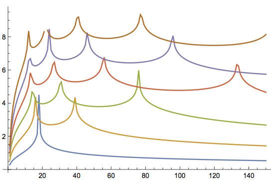
Figure 3: Plot of the giving the accuracy of the double-scaled estimates of the MMP function through N⁵LO. The quantity being plotted is $-{1\over{{\rm Log}[10]}}$ the logarithm of the relative error in the estimate of the MMP function. The horizontal axis is $n$, and the vertical axis is $-{1\over{{\rm Log}[10]}}\,{\rm Log}\left[\,{{|q_{n}^{({\rm{\textsc{mmp}}})}-(q_{n}^{({\rm{\textsc{mmp}}})})_{{\rm{estimate}}}|}\over{|q_{n}^{({\rm{\textsc{mmp}}})}|}}\,\right]$ The LO, NLO, N²LO, N³LO, N⁴LO and N⁵LO double-scaled estimates are given by the blue, yellow, green, red, and purple, and brown dots respectively. The upward spikes represent ”accidental accuracies” in which an estimate transitions between slightly overestimating and slightly underestimating the exact result as $n$ is varied, generating an atypically precise agreement between a given estimate and the exact amplitude, in some small range of $n$.

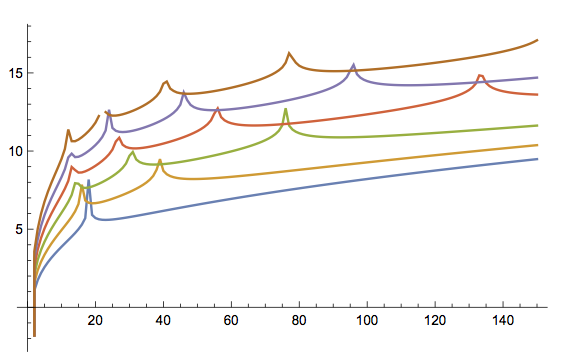
Figure 4: Plot of the giving the accuracy of the double-scaled estimates of the full log of the scheme-independent correlator $\tilde{G}_{2n}\equiv{{G_{2n}}\over{(G_{2})^{n}}}=e^{q_{n}-n\,q_{1}+(n-1)q_{0}}$, through N⁵LO. The quantity being plotted is $-{1\over{{\rm Log}[10]}}$ the logarithm of the relative error in the estimate of the MMP function. The horizontal axis is $n$, and the vertical axis is $-{1\over{{\rm Log}[10]}}\,{\rm Log}\left[\,{{|q_{n}-(q_{n})_{{\rm{estimate}}}|}\over{|q_{n}-n\,q_{1}+(n-1)q_{0}|}}\,\right]$ The leading-order, NLO, N²LO, N³LO, N⁴LO and N⁵LO estimates are given by the blue, yellow, green, red, and purple, and brown dots respectively. The upward spikes represent ”accidental accuracies” in which an estimate transitions between slightly overestimating and slightly underestimating the exact result as $n$ is varied, generating an atypically precise agreement between a given estimate and the exact amplitude, in some small range of $n$.

6.3 Table of values of the double-scaled (i.e. fixed-${\color[rgb]{0.808594,0.242188,0.46875}{\lambda}}$) large-charge asymptotic estimates at $\tau={{25}\over\pi}\,i$ up to $n=150$

	$F_{[{0}]}[{\color[rgb]{0.808594,0.242188,0.46875}{\lambda}}]$	${{\rm estimate~{}incl.}\atop{n^{-1}F_{[{1}]}[{\color[rgb]{0.808594,0.242188,0.46875}{\lambda}}]}}$	${{\rm estimate~{}incl.}\atop{n^{-2}F_{[{2}]}[{\color[rgb]{0.808594,0.242188,0.46875}{\lambda}}]}}$	${{\rm estimate~{}incl.}\atop{n^{-3}F_{[{3}]}[{\color[rgb]{0.808594,0.242188,0.46875}{\lambda}}]}}$	${{\rm estimate~{}incl.}\atop{n^{-4}F_{[{4}]}[{\color[rgb]{0.808594,0.242188,0.46875}{\lambda}}]}}$	${{\rm estimate~{}incl.}\atop{n^{-5}F_{[{5}]}[{\color[rgb]{0.808594,0.242188,0.46875}{\lambda}}]}}$	$(q_{n}^{({\rm{\textsc{mmp}}})})_{{\rm{exact}}}$
1	0.6515789571	0.3106159884	0.4912085899	0.3869269511	0.4513455344	0.4099885449	0.4263073863
2	0.3946733263	0.2608832307	0.3020903723	0.2894178806	0.2934159952	0.2921249755	0.2924432054
3	0.2711221920	0.2007750251	0.2169181342	0.2133789929	0.2141499819	0.2139812813	0.2140116919
4	0.1980089293	0.1562620119	0.1640670070	0.1627032722	0.1629353694	0.1628962899	0.1629019007
5	0.1502153430	0.1237476447	0.1279557008	0.1273368696	0.1274245447	0.1274123721	0.1274138410
6	0.1170270973	0.09954831105	0.1019669053	0.1016586081	0.1016962711	0.1016917835	0.1016922546
7	0.09300855834	0.08115719284	0.08260296089	0.08244065014	0.08245807861	0.08245625608	0.08245642599
8	0.07508946762	0.06691661367	0.06780122735	0.06771312872	0.06772151249	0.06772073565	0.06772080050
9	0.06140276891	0.05571131925	0.05625864419	0.05621029365	0.05621436529	0.05621403196	0.05621405675
10	0.05074985468	0.04677219216	0.04711083791	0.04708452067	0.04708645350	0.04708631681	0.04708632558
11	0.04232850769	0.03955582885	0.03976277450	0.03974892486	0.03974977625	0.03974972807	0.03974973039
12	0.03558371710	0.03366981364	0.03379259457	0.03378585902	0.03378616421	0.03378615512	0.03378615497
13	0.03012096484	0.02882524012	0.02889391825	0.02889122382	0.02889126049	0.02889126744	0.02889126648
14	0.02565341289	0.02480576447	0.02483969766	0.02483925094	0.02483916477	0.02483917702	0.02483917594
15	0.02196848039	0.02144693696	0.02145875613	0.02145950165	0.02145936873	0.02145938143	0.02145938050
16	0.01890600199	0.01862208600	0.01862010631	0.01862142301	0.01862128213	0.01862129330	0.01862129258
17	0.01634355964	0.01623248103	0.01622220237	0.01622372867	0.01622359848	0.01622360749	0.01622360696
18	0.01418639766	0.01420035157	0.01418541289	0.01418694359	0.01418683189	0.01418683872	0.01418683837
19	0.01236034544	0.01246385154	0.01244664912	0.01244807353	0.01244798241	0.01244798732	0.01244798710
20	0.01080676066	0.01097337293	0.01095546710	0.01095673146	0.01095666011	0.01095666344	0.01095666332
21	0.009478857881	0.009688810997	0.009671197203	0.009672281587	0.009672227894	0.009672229973	0.009672229925
22	0.008339004755	0.008577510675	0.008560802010	0.008561706111	0.008561667481	0.008561668609	0.008561668609
23	0.007356704985	0.007612707402	0.007597258612	0.007597992954	0.007597966770	0.007597967198	0.007597967228
24	0.006507076091	0.006772331309	0.006758323571	0.006758904129	0.006758887969	0.006758887898	0.006758887946
25	0.005769688366	0.006038081569	0.006025580719	0.006026025648	0.006026017381	0.006026016969	0.006026017027
26	0.005127670735	0.005394703710	0.005383700338	0.005384028043	0.005384025851	0.005384025221	0.005384025281
27	0.004567016031	0.004829420924	0.004819857988	0.004820086027	0.004820088395	0.004820087638	0.004820087697
28	0.004076036781	0.004331483276	0.004323275076	0.004323419587	0.004323425275	0.004323424459	0.004323424514
29	0.003644935681	0.003891807929	0.003884853075	0.003884928518	0.003884936528	0.003884935700	0.003884935751
30	0.003265464184	0.003502690183	0.003496880366	0.003496899468	0.003496909006	0.003496908200	0.003496908245
31	0.002930649381	0.003157570017	0.003152795854	0.003152769661	0.003152780103	0.003152779343	0.003152779381
32	0.002634574151	0.002850842411	0.002846997247	0.002846935240	0.002846946105	0.002846945404	0.002846945436
33	0.002372199210	0.002577702455	0.002574684734	0.002574594972	0.002574605896	0.002574605261	0.002574605288
34	0.002139218286	0.002334018223	0.002331732873	0.002331622153	0.002331632862	0.002331632298	0.002331632319
35	0.001931939664	0.002116225963	0.002114585104	0.002114459111	0.002114469409	0.002114468915	0.002114468932

Table 13: The successive refined estimates for the massive macroscopic propagation function $q_{n}^{({\rm{\textsc{mmp}}})}\equiv q_{n}-q_{n}^{({\rm{eft}})}$, at the coupling $\tau={{25i}\over{\pi}}$. The first column represents the strict infinite-$n$ limit at fixed double-scaling parameter ${\color[rgb]{0.808594,0.242188,0.46875}{\lambda}}$, $q_{n}^{({\rm{\textsc{mmp}}})}\simeq F_{[{0}]}[{\color[rgb]{0.808594,0.242188,0.46875}{\lambda}}]=F^{{\rm{inst}}}_{({\hbox{\tiny{ref. \cite[cite]{[\@@bibref{}{Grassi:2019txd}{}{}]}}}})}[{\color[rgb]{0.808594,0.242188,0.46875}{\lambda}}]$. The next five columns represent this approximation corrected by adding successive terms $n^{-k}\,F_{[{k}]}[{\color[rgb]{0.808594,0.242188,0.46875}{\lambda}}]$ for $k=1,\cdots 5$. The last column is the exact result as computed [91] following the method of [14].

	$F_{[{0}]}[{\color[rgb]{0.808594,0.242188,0.46875}{\lambda}}]$	${{\rm estimate~{}incl.}\atop{n^{-1}F_{[{1}]}[{\color[rgb]{0.808594,0.242188,0.46875}{\lambda}}]}}$	${{\rm estimate~{}incl.}\atop{n^{-2}F_{[{2}]}[{\color[rgb]{0.808594,0.242188,0.46875}{\lambda}}]}}$	${{\rm estimate~{}incl.}\atop{n^{-3}F_{[{3}]}[{\color[rgb]{0.808594,0.242188,0.46875}{\lambda}}]}}$	${{\rm estimate~{}incl.}\atop{n^{-4}F_{[{4}]}[{\color[rgb]{0.808594,0.242188,0.46875}{\lambda}}]}}$	${{\rm estimate~{}incl.}\atop{n^{-5}F_{[{5}]}[{\color[rgb]{0.808594,0.242188,0.46875}{\lambda}}]}}$	$(q_{n}^{({\rm{\textsc{mmp}}})})_{{\rm{exact}}}$
36	0.001747188853	0.001921243312	0.001920166501	0.001920029953	0.001920039702	0.001920039277	0.001920039289
37	0.001582228233	0.001746397130	0.001745811295	0.001745668079	0.001745677189	0.001745676828	0.001745676837
38	0.001434690459	0.001589363259	0.001589202444	0.001589055732	0.001589064149	0.001589063848	0.001589063854
39	0.001302523033	0.001448116056	0.001448321035	0.001448173393	0.001448181090	0.001448180845	0.001448180848
40	0.001183942002	0.001320885953	0.001321403782	0.001321257261	0.001321264234	0.001321264039	0.001321264040
41	0.001077393142	0.001206123664	0.001206907196	0.001206763414	0.001206769674	0.001206769523	0.001206769522
42	0.0009815192976	0.001102469881	0.001103477277	0.001103337490	0.001103343060	0.001103342948	0.001103342946
43	0.0008951328279	0.001008729558	0.001009923809	0.001009788968	0.001009793878	0.001009793802	0.001009793798
44	0.0008171922687	0.0009238500137	0.0009251984792	0.0009250692846	0.0009250735723	0.0009250735254	0.0009250735212
45	0.0007467825211	0.0008469022370	0.0008483762128	0.0008482531567	0.0008482568617	0.0008482568405	0.0008482568358
46	0.0006830979808	0.0007770648850	0.0007786391999	0.0007785226037	0.0007785257677	0.0007785257685	0.0007785257633
47	0.0006254281327	0.0007136105490	0.0007152631935	0.0007151532393	0.0007151559046	0.0007151559239	0.0007151559185
48	0.0005731452189	0.0006558939394	0.0006576057257	0.0006575024833	0.0006575046917	0.0006575047264	0.0006575047208
49	0.0005256936560	0.0006033416976	0.0006050959505	0.0006049993989	0.0006050011913	0.0006050012386	0.0006050012329
50	0.0004825809307	0.0005554435896	0.0005572258663	0.0005571359133	0.0005571373289	0.0005571373863	0.0005571373807
51	0.0004433697498	0.0005117448790	0.0005135427166	0.0005134592139	0.0005134602901	0.0005134603555	0.0005134603500
52	0.0004076712568	0.0004718397065	0.0004736423948	0.0004735651513	0.0004735659233	0.0004735659948	0.0004735659895
53	0.0003751391572	0.0004353653317	0.0004371637095	0.0004370925022	0.0004370930031	0.0004370930790	0.0004370930739
54	0.0003454646213	0.0004019971155	0.0004037833887	0.0004037179712	0.0004037182317	0.0004037183106	0.0004037183057
55	0.0003183718512	0.0003714441394	0.0003732117176	0.0003731518279	0.0003731518766	0.0003731519572	0.0003731519527
56	0.0002936142202	0.0003434453736	0.0003451887254	0.0003451340919	0.0003451339549	0.0003451340363	0.0003451340321
57	0.0002709709024	0.0003177663198	0.0003194808436	0.0003194311898	0.0003194308912	0.0003194309725	0.0003194309685
58	0.0002502439267	0.0002941960646	0.0002958779737	0.0002958330222	0.0002958325840	0.0002958326644	0.0002958326607
59	0.0002312555960	0.0002725446892	0.0002741909098	0.0002741503855	0.0002741498277	0.0002741499066	0.0002741499032
60	0.0002138462236	0.0002526409886	0.0002542490695	0.0002542127019	0.0002542120425	0.0002542121195	0.0002542121164
61	0.0001978721442	0.0002343304601	0.0002358984921	0.0002358660175	0.0002358652730	0.0002358653476	0.0002358653448
62	0.0001832039628	0.0002174735268	0.0002190000722	0.0002189712350	0.0002189704201	0.0002189704921	0.0002189704896
63	0.0001697250120	0.0002019439669	0.0002034279965	0.0002034025502	0.0002034016782	0.0002034017473	0.0002034017450
64	0.0001573299900	0.0001876275216	0.0001890683593	0.0001890460675	0.0001890451501	0.0001890452162	0.0001890452141
65	0.0001459237564	0.0001744206612	0.0001758179350	0.0001757985716	0.0001757976195	0.0001757976824	0.0001757976806
66	0.0001354202667	0.0001622294889	0.0001635830878	0.0001635664377	0.0001635654603	0.0001635655198	0.0001635655183
67	0.0001257416277	0.0001509687666	0.0001522788025	0.0001522646613	0.0001522636668	0.0001522637231	0.0001522637217
68	0.0001168172587	0.0001405610465	0.0001418278208	0.0001418159951	0.0001418149908	0.0001418150437	0.0001418150425
69	0.0001085831469	0.0001309358982	0.0001321598721	0.0001321501793	0.0001321491716	0.0001321492212	0.0001321492202
70	0.0001009811840	0.0001220292180	0.0001232109870	0.0001232032549	0.0001232022494	0.0001232022959	0.0001232022950

Table 14: The successive refined estimates for the massive macroscopic propagation function $q_{n}^{({\rm{\textsc{mmp}}})}\equiv q_{n}-q_{n}^{({\rm{eft}})}$, at the coupling $\tau={{25i}\over{\pi}}$. The first column represents the strict infinite-$n$ limit at fixed double-scaling parameter ${\color[rgb]{0.808594,0.242188,0.46875}{\lambda}}$, $q_{n}^{({\rm{\textsc{mmp}}})}\simeq F_{[{0}]}[{\color[rgb]{0.808594,0.242188,0.46875}{\lambda}}]=F^{{\rm{inst}}}_{({\hbox{\tiny{ref. \cite[cite]{[\@@bibref{}{Grassi:2019txd}{}{}]}}}})}[{\color[rgb]{0.808594,0.242188,0.46875}{\lambda}}]$. The next five columns represent this approximation corrected by adding successive terms $n^{-k}\,F_{[{k}]}[{\color[rgb]{0.808594,0.242188,0.46875}{\lambda}}]$ for $k=1,\cdots 5$. The last column is the exact result as computed [91] following the method of [14].

	$F_{[{0}]}[{\color[rgb]{0.808594,0.242188,0.46875}{\lambda}}]$	${{\rm estimate~{}incl.}\atop{n^{-1}F_{[{1}]}[{\color[rgb]{0.808594,0.242188,0.46875}{\lambda}}]}}$	${{\rm estimate~{}incl.}\atop{n^{-2}F_{[{2}]}[{\color[rgb]{0.808594,0.242188,0.46875}{\lambda}}]}}$	${{\rm estimate~{}incl.}\atop{n^{-3}F_{[{3}]}[{\color[rgb]{0.808594,0.242188,0.46875}{\lambda}}]}}$	${{\rm estimate~{}incl.}\atop{n^{-4}F_{[{4}]}[{\color[rgb]{0.808594,0.242188,0.46875}{\lambda}}]}}$	${{\rm estimate~{}incl.}\atop{n^{-5}F_{[{5}]}[{\color[rgb]{0.808594,0.242188,0.46875}{\lambda}}]}}$	$(q_{n}^{({\rm{\textsc{mmp}}})})_{{\rm{exact}}}$
71	0.00009395857627	0.0001137826120	0.0001149228833	0.0001149169501	0.0001149159516	0.0001149159950	0.0001149159943
72	0.00008746731725	0.0001061428449	0.0001072424172	0.0001072381311	0.0001072371438	0.0001072371840	0.0001072371835
73	0.00008146371776	0.00009906134541	0.0001001210918	0.0001001183104	0.0001001173379	0.0001001173752	0.0001001173747
74	0.00007590798546	0.00009249376341	0.00009351461614	0.00009351320646	0.00009351225181	0.00009351228623	0.00009351228591
75	0.00007076384866	0.00008639957275	0.00008738251023	0.00008738234799	0.00008738141374	0.00008738144540	0.00008738144519
76	0.00006599821932	0.00008074171402	0.00008168774925	0.00008168871860	0.00008168780685	0.00008168783588	0.00008168783576
77	0.00006158089089	0.00007548627365	0.00007639644430	0.00007639843736	0.00007639754985	0.00007639757635	0.00007639757633
78	0.00005748426706	0.00007060219491	0.00007147755480	0.00007148047123	0.00007147960935	0.00007147963346	0.00007147963351
79	0.00005368311801	0.00006606101768	0.00006690262936	0.00006690637599	0.00006690554082	0.00006690556266	0.00006690556278
80	0.00005015436127	0.00006183664370	0.00006264557213	0.00006265006256	0.00006264925490	0.00006264927459	0.00006264927477
81	0.00004687686437	0.00005790512479	0.00005868243193	0.00005868758610	0.00005868680653	0.00005868682419	0.00005868682442
82	0.00004383126706	0.00005424447148	0.00005499121170	0.00005499695553	0.00005499620441	0.00005499622015	0.00005499622043
83	0.00004099982096	0.00005083448000	0.00005155169620	0.00005155796124	0.00005155723874	0.00005155725269	0.00005155725300
84	0.00003836624486	0.00004765657580	0.00004834529612	0.00004835201920	0.00004835132533	0.00004835133759	0.00004835133795
85	0.00003591559396	0.00004469367174	0.00004535490689	0.00004536202976	0.00004536136441	0.00004536137509	0.00004536137547
86	0.00003363414166	0.00004193003964	0.00004256478065	0.00004257224970	0.00004257161261	0.00004257162182	0.00004257162223
87	0.00003150927258	0.00003935119372	0.00003996041018	0.00003996817610	0.00003996756692	0.00003996757476	0.00003996757518
88	0.00002952938572	0.00003694378487	0.00003752842343	0.00003753644094	0.00003753585923	0.00003753586580	0.00003753586624
89	0.00002768380662	0.00003469550447	0.00003525648777	0.00003526471537	0.00003526416061	0.00003526416600	0.00003526416645
90	0.00002596270774	0.00003259499712	0.00003313322295	0.00003314162260	0.00003314109423	0.00003314109852	0.00003314109898
91	0.00002435703620	0.00003063178108	0.00003114812176	0.00003115665871	0.00003115615610	0.00003115615938	0.00003115615984
92	0.00002285844809	0.00002879617598	0.00002929147799	0.00002930012051	0.00002929964298	0.00002929964533	0.00002929964580
93	0.00002145924875	0.00002707923686	0.00002755432063	0.00002756303979	0.00002756258666	0.00002756258815	0.00002756258862
94	0.00002015233856	0.00002547269406	0.00002592835392	0.00002593712343	0.00002593669396	0.00002593669467	0.00002593669514
95	0.00001893116342	0.00002396889846	0.00002440590270	0.00002441469868	0.00002441429212	0.00002441429211	0.00002441429258
96	0.00001778966979	0.00002256077135	0.00002297986244	0.00002298866325	0.00002298827885	0.00002298827819	0.00002298827865
97	0.00001672226361	0.00002124175876	0.00002164365363	0.00002165243972	0.00002165207670	0.00002165207545	0.00002165207590
98	0.00001572377287	0.00002000578969	0.00002039118006	0.00002039993379	0.00002039959140	0.00002039958960	0.00002039959005
99	0.00001478941348	0.00001884723783	0.00001921679069	0.00001922549621	0.00001922517367	0.00001922517139	0.00001922517183
100	0.00001391475800	0.00001776088663	0.00001811524470	0.00001812388779	0.00001812358435	0.00001812358164	0.00001812358207
101	0.00001309570717	0.00001674189727	0.00001708167952	0.00001709024751	0.00001708996240	0.00001708995929	0.00001708995971
102	0.00001232846384	0.00001578577929	0.00001611158153	0.00001612006311	0.00001611979559	0.00001611979214	0.00001611979255
103	0.00001160950905	0.00001488836370	0.00001520075917	0.00001520914432	0.00001520889367	0.00001520888991	0.00001520889031
104	0.00001093558026	0.00001404577830	0.00001434531825	0.00001435359817	0.00001435336365	0.00001435335962	0.00001435336001
105	0.00001030365130	0.00001325442503	0.00001354163939	0.00001354980634	0.00001354958725	0.00001354958299	0.00001354958336
106	9.710914034$\times 10^{-6}$	0.00001251095916	0.00001278635714	0.00001279440439	0.00001279420005	0.00001279419559	0.00001279419595
107	9.154761542$\times 10^{-6}$	0.00001181227019	0.00001207634095	0.00001208426269	0.00001208407243	0.00001208406779	0.00001208406814
108	8.632772702$\times 10^{-6}$	0.00001115546427	0.00001140867755	0.00001141646882	0.00001141629198	0.00001141628720	0.00001141628753
109	8.142698011$\times 10^{-6}$	0.00001053784805	0.00001078065480	0.00001078831140	0.00001078814736	0.00001078814245	0.00001078814278
110	7.682446573$\times 10^{-6}$	9.956913799$\times 10^{-6}$	0.00001018974683	0.00001019726528	0.00001019711342	0.00001019710841	0.00001019710872

Table 15: The successive refined estimates for the massive macroscopic propagation function $q_{n}^{({\rm{\textsc{mmp}}})}\equiv q_{n}-q_{n}^{({\rm{eft}})}$, at the coupling $\tau={{25i}\over{\pi}}$. The first column represents the strict infinite-$n$ limit at fixed double-scaling parameter ${\color[rgb]{0.808594,0.242188,0.46875}{\lambda}}$, $q_{n}^{({\rm{\textsc{mmp}}})}\simeq F_{[{0}]}[{\color[rgb]{0.808594,0.242188,0.46875}{\lambda}}]=F^{{\rm{inst}}}_{({\hbox{\tiny{ref. \cite[cite]{[\@@bibref{}{Grassi:2019txd}{}{}]}}}})}[{\color[rgb]{0.808594,0.242188,0.46875}{\lambda}}]$. The next five columns represent this approximation corrected by adding successive terms $n^{-k}\,F_{[{k}]}[{\color[rgb]{0.808594,0.242188,0.46875}{\lambda}}]$ for $k=1,\cdots 5$. The last column is the exact result as computed [91] following the method of [14].

	$F_{[{0}]}[{\color[rgb]{0.808594,0.242188,0.46875}{\lambda}}]$	${{\rm estimate~{}incl.}\atop{n^{-1}F_{[{1}]}[{\color[rgb]{0.808594,0.242188,0.46875}{\lambda}}]}}$	${{\rm estimate~{}incl.}\atop{n^{-2}F_{[{2}]}[{\color[rgb]{0.808594,0.242188,0.46875}{\lambda}}]}}$	${{\rm estimate~{}incl.}\atop{n^{-3}F_{[{3}]}[{\color[rgb]{0.808594,0.242188,0.46875}{\lambda}}]}}$	${{\rm estimate~{}incl.}\atop{n^{-4}F_{[{4}]}[{\color[rgb]{0.808594,0.242188,0.46875}{\lambda}}]}}$	${{\rm estimate~{}incl.}\atop{n^{-5}F_{[{5}]}[{\color[rgb]{0.808594,0.242188,0.46875}{\lambda}}]}}$	$(q_{n}^{({\rm{\textsc{mmp}}})})_{{\rm{exact}}}$
111	7.250074141$\times 10^{-6}$	9.410325706$\times 10^{-6}$	9.633600332$\times 10^{-6}$	9.640977777$\times 10^{-6}$	9.640837502$\times 10^{-6}$	9.640832419$\times 10^{-6}$	9.640832718$\times 10^{-6}$
112	6.843772122$\times 10^{-6}$	8.895907290$\times 10^{-6}$	9.110021916$\times 10^{-6}$	9.117256104$\times 10^{-6}$	9.117126842$\times 10^{-6}$	9.117121703$\times 10^{-6}$	9.117121989$\times 10^{-6}$
113	6.461857457$\times 10^{-6}$	8.411629758$\times 10^{-6}$	8.616966505$\times 10^{-6}$	8.624055717$\times 10^{-6}$	8.623936916$\times 10^{-6}$	8.623931737$\times 10^{-6}$	8.623932012$\times 10^{-6}$
114	6.102763311$\times 10^{-6}$	7.955601288$\times 10^{-6}$	8.152526593$\times 10^{-6}$	8.159469597$\times 10^{-6}$	8.159360721$\times 10^{-6}$	8.159355520$\times 10^{-6}$	8.159355782$\times 10^{-6}$
115	5.765030502$\times 10^{-6}$	7.526057145$\times 10^{-6}$	7.714922340$\times 10^{-6}$	7.721718345$\times 10^{-6}$	7.721618881$\times 10^{-6}$	7.721613674$\times 10^{-6}$	7.721613924$\times 10^{-6}$
116	5.447299596$\times 10^{-6}$	7.121350554$\times 10^{-6}$	7.302492439$\times 10^{-6}$	7.309141055$\times 10^{-6}$	7.309050508$\times 10^{-6}$	7.309045308$\times 10^{-6}$	7.309045546$\times 10^{-6}$
117	5.148303631$\times 10^{-6}$	6.739944272$\times 10^{-6}$	6.913685667$\times 10^{-6}$	6.920186869$\times 10^{-6}$	6.920104763$\times 10^{-6}$	6.920099582$\times 10^{-6}$	6.920099809$\times 10^{-6}$
118	4.866861398$\times 10^{-6}$	6.380402806$\times 10^{-6}$	6.547053095$\times 10^{-6}$	6.553407181$\times 10^{-6}$	6.553333061$\times 10^{-6}$	6.553327910$\times 10^{-6}$	6.553328125$\times 10^{-6}$
119	4.601871247$\times 10^{-6}$	6.041385219$\times 10^{-6}$	6.201240871$\times 10^{-6}$	6.207448435$\times 10^{-6}$	6.207381862$\times 10^{-6}$	6.207376753$\times 10^{-6}$	6.207376957$\times 10^{-6}$
120	4.352305373$\times 10^{-6}$	5.721638475$\times 10^{-6}$	5.874983557$\times 10^{-6}$	5.881045458$\times 10^{-6}$	5.880986013$\times 10^{-6}$	5.880980953$\times 10^{-6}$	5.880981146$\times 10^{-6}$
121	4.117204528$\times 10^{-6}$	5.419991292$\times 10^{-6}$	5.567097960$\times 10^{-6}$	5.573015291$\times 10^{-6}$	5.572962572$\times 10^{-6}$	5.572957570$\times 10^{-6}$	5.572957753$\times 10^{-6}$
122	3.895673153$\times 10^{-6}$	5.135348446$\times 10^{-6}$	5.276477422$\times 10^{-6}$	5.282251488$\times 10^{-6}$	5.282205110$\times 10^{-6}$	5.282200173$\times 10^{-6}$	5.282200346$\times 10^{-6}$
123	3.686874861$\times 10^{-6}$	4.866685498$\times 10^{-6}$	5.002086533$\times 10^{-6}$	5.007718826$\times 10^{-6}$	5.007678421$\times 10^{-6}$	5.007673556$\times 10^{-6}$	5.007673719$\times 10^{-6}$
124	3.490028274$\times 10^{-6}$	4.613043919$\times 10^{-6}$	4.742956236$\times 10^{-6}$	4.748448413$\times 10^{-6}$	4.748413630$\times 10^{-6}$	4.748408842$\times 10^{-6}$	4.748408996$\times 10^{-6}$
125	3.304403163$\times 10^{-6}$	4.373526560$\times 10^{-6}$	4.498179287$\times 10^{-6}$	4.503533150$\times 10^{-6}$	4.503503654$\times 10^{-6}$	4.503498948$\times 10^{-6}$	4.503499093$\times 10^{-6}$
126	3.129316885$\times 10^{-6}$	4.147293465$\times 10^{-6}$	4.266906049$\times 10^{-6}$	4.272123528$\times 10^{-6}$	4.272098998$\times 10^{-6}$	4.272094378$\times 10^{-6}$	4.272094514$\times 10^{-6}$
127	2.964131077$\times 10^{-6}$	3.933557980$\times 10^{-6}$	4.048340586$\times 10^{-6}$	4.053423721$\times 10^{-6}$	4.053403852$\times 10^{-6}$	4.053399322$\times 10^{-6}$	4.053399450$\times 10^{-6}$
128	2.808248593$\times 10^{-6}$	3.731583150$\times 10^{-6}$	3.841737048$\times 10^{-6}$	3.846687974$\times 10^{-6}$	3.846672474$\times 10^{-6}$	3.846668038$\times 10^{-6}$	3.846668157$\times 10^{-6}$
129	2.661110677$\times 10^{-6}$	3.540678374$\times 10^{-6}$	3.646396307$\times 10^{-6}$	3.651217239$\times 10^{-6}$	3.651205831$\times 10^{-6}$	3.651201491$\times 10^{-6}$	3.651201602$\times 10^{-6}$
130	2.522194331$\times 10^{-6}$	3.360196292$\times 10^{-6}$	3.461662834$\times 10^{-6}$	3.466356057$\times 10^{-6}$	3.466348478$\times 10^{-6}$	3.466344235$\times 10^{-6}$	3.466344339$\times 10^{-6}$
131	2.391009879$\times 10^{-6}$	3.189529909$\times 10^{-6}$	3.286921808$\times 10^{-6}$	3.291489661$\times 10^{-6}$	3.291485659$\times 10^{-6}$	3.291481516$\times 10^{-6}$	3.291481613$\times 10^{-6}$
132	2.267098709$\times 10^{-6}$	3.028109907$\times 10^{-6}$	3.121596413$\times 10^{-6}$	3.126041283$\times 10^{-6}$	3.126040619$\times 10^{-6}$	3.126036577$\times 10^{-6}$	3.126036667$\times 10^{-6}$
133	2.150031176$\times 10^{-6}$	2.875402160$\times 10^{-6}$	2.965145344$\times 10^{-6}$	2.969469651$\times 10^{-6}$	2.969472099$\times 10^{-6}$	2.969468159$\times 10^{-6}$	2.969468243$\times 10^{-6}$
134	2.039404656$\times 10^{-6}$	2.730905416$\times 10^{-6}$	2.817060471$\times 10^{-6}$	2.821266664$\times 10^{-6}$	2.821272008$\times 10^{-6}$	2.821268170$\times 10^{-6}$	2.821268247$\times 10^{-6}$
135	1.934841737$\times 10^{-6}$	2.594149141$\times 10^{-6}$	2.676864676$\times 10^{-6}$	2.680955221$\times 10^{-6}$	2.680963258$\times 10^{-6}$	2.680959523$\times 10^{-6}$	2.680959594$\times 10^{-6}$
136	1.835988542$\times 10^{-6}$	2.464691520$\times 10^{-6}$	2.544109839$\times 10^{-6}$	2.548087215$\times 10^{-6}$	2.548097750$\times 10^{-6}$	2.548094118$\times 10^{-6}$	2.548094183$\times 10^{-6}$
137	1.742513168$\times 10^{-6}$	2.342117589$\times 10^{-6}$	2.418374960$\times 10^{-6}$	2.422241650$\times 10^{-6}$	2.422254499$\times 10^{-6}$	2.422250970$\times 10^{-6}$	2.422251029$\times 10^{-6}$
138	1.654104234$\times 10^{-6}$	2.226037502$\times 10^{-6}$	2.299264412$\times 10^{-6}$	2.303022899$\times 10^{-6}$	2.303037888$\times 10^{-6}$	2.303034460$\times 10^{-6}$	2.303034515$\times 10^{-6}$
139	1.570469537$\times 10^{-6}$	2.116084908$\times 10^{-6}$	2.186406315$\times 10^{-6}$	2.190059074$\times 10^{-6}$	2.190076038$\times 10^{-6}$	2.190072712$\times 10^{-6}$	2.190072761$\times 10^{-6}$
140	1.491334790$\times 10^{-6}$	2.011915454$\times 10^{-6}$	2.079451018$\times 10^{-6}$	2.083000514$\times 10^{-6}$	2.083019296$\times 10^{-6}$	2.083016070$\times 10^{-6}$	2.083016115$\times 10^{-6}$
141	1.416442463$\times 10^{-6}$	1.913205372$\times 10^{-6}$	1.978069686$\times 10^{-6}$	1.981518367$\times 10^{-6}$	1.981538820$\times 10^{-6}$	1.981535694$\times 10^{-6}$	1.981535734$\times 10^{-6}$
142	1.345550688$\times 10^{-6}$	1.819650176$\times 10^{-6}$	1.881952982$\times 10^{-6}$	1.885303277$\times 10^{-6}$	1.885325262$\times 10^{-6}$	1.885322234$\times 10^{-6}$	1.885322270$\times 10^{-6}$
143	1.278432254$\times 10^{-6}$	1.730963443$\times 10^{-6}$	1.790809839$\times 10^{-6}$	1.794064153$\times 10^{-6}$	1.794087538$\times 10^{-6}$	1.794084607$\times 10^{-6}$	1.794084639$\times 10^{-6}$
144	1.214873661$\times 10^{-6}$	1.646875668$\times 10^{-6}$	1.704366308$\times 10^{-6}$	1.707527023$\times 10^{-6}$	1.707551682$\times 10^{-6}$	1.707548848$\times 10^{-6}$	1.707548876$\times 10^{-6}$
145	1.154674239$\times 10^{-6}$	1.567133209$\times 10^{-6}$	1.622364496$\times 10^{-6}$	1.625433961$\times 10^{-6}$	1.625459778$\times 10^{-6}$	1.625457038$\times 10^{-6}$	1.625457062$\times 10^{-6}$
146	1.097645335$\times 10^{-6}$	1.491497291$\times 10^{-6}$	1.544561558$\times 10^{-6}$	1.547542093$\times 10^{-6}$	1.547568957$\times 10^{-6}$	1.547566309$\times 10^{-6}$	1.547566330$\times 10^{-6}$
147	1.043609546$\times 10^{-6}$	1.419743085$\times 10^{-6}$	1.470728767$\times 10^{-6}$	1.473622660$\times 10^{-6}$	1.473650465$\times 10^{-6}$	1.473647908$\times 10^{-6}$	1.473647926$\times 10^{-6}$
148	9.924000085$\times 10^{-7}$	1.351658836$\times 10^{-6}$	1.400650644$\times 10^{-6}$	1.403460146$\times 10^{-6}$	1.403488795$\times 10^{-6}$	1.403486327$\times 10^{-6}$	1.403486342$\times 10^{-6}$
149	9.438597330$\times 10^{-7}$	1.287045064$\times 10^{-6}$	1.334124140$\times 10^{-6}$	1.336851466$\times 10^{-6}$	1.336880866$\times 10^{-6}$	1.336878486$\times 10^{-6}$	1.336878498$\times 10^{-6}$
150	8.978409857$\times 10^{-7}$	1.225713802$\times 10^{-6}$	1.270957877$\times 10^{-6}$	1.273605203$\times 10^{-6}$	1.273635268$\times 10^{-6}$	1.273632973$\times 10^{-6}$	1.273632982$\times 10^{-6}$

Table 16: The successive refined estimates for the massive macroscopic propagation function $q_{n}^{({\rm{\textsc{mmp}}})}\equiv q_{n}-q_{n}^{({\rm{eft}})}$, at the coupling $\tau={{25i}\over{\pi}}$. The first column represents the strict infinite-$n$ limit at fixed double-scaling parameter ${\color[rgb]{0.808594,0.242188,0.46875}{\lambda}}$, $q_{n}^{({\rm{\textsc{mmp}}})}\simeq F_{[{0}]}[{\color[rgb]{0.808594,0.242188,0.46875}{\lambda}}]=F^{{\rm{inst}}}_{({\hbox{\tiny{ref. \cite[cite]{[\@@bibref{}{Grassi:2019txd}{}{}]}}}})}[{\color[rgb]{0.808594,0.242188,0.46875}{\lambda}}]$. The next five columns represent this approximation corrected by adding successive terms $n^{-k}\,F_{[{k}]}[{\color[rgb]{0.808594,0.242188,0.46875}{\lambda}}]$ for $k=1,\cdots 5$. The last column is the exact result as computed [91] following the method of [14].

6.4 Tables listing the accuracy of the double-scaled (i.e. fixed-${\color[rgb]{0.808594,0.242188,0.46875}{\lambda}}$) large-charge asymptotic estimates at $\tau={{25}\over\pi}\,i$, up to $n=150$

	${{{\rm accuracy~{}of}}\atop{F_{[{0}]}[{\color[rgb]{0.808594,0.242188,0.46875}{\lambda}}]}}$	${{\rm accuracy~{}incl.}\atop{n^{-1}F_{[{1}]}[{\color[rgb]{0.808594,0.242188,0.46875}{\lambda}}]}}$	${{\rm accuracy~{}incl.}\atop{n^{-2}F_{[{2}]}[{\color[rgb]{0.808594,0.242188,0.46875}{\lambda}}]}}$	${{\rm accuracy~{}incl.}\atop{n^{-3}F_{[{3}]}[{\color[rgb]{0.808594,0.242188,0.46875}{\lambda}}]}}$	${{\rm accuracy~{}incl.}\atop{n^{-4}F_{[{4}]}[{\color[rgb]{0.808594,0.242188,0.46875}{\lambda}}]}}$	${{\rm accuracy~{}incl.}\atop{n^{-5}F_{[{5}]}[{\color[rgb]{0.808594,0.242188,0.46875}{\lambda}}]}}$
1	0.2770	0.5664	0.8175	1.034	1.231	1.417
2	0.4565	0.9669	1.482	1.985	2.478	2.963
3	0.5737	1.209	1.867	2.529	3.190	3.847
4	0.6665	1.390	2.146	2.914	3.687	4.463
5	0.7473	1.541	2.371	3.219	4.076	4.938
6	0.8216	1.676	2.569	3.480	4.403	5.334
7	0.8929	1.803	2.750	3.718	4.698	5.686
8	0.9633	1.925	2.925	3.946	4.978	6.019
9	1.035	2.049	3.101	4.174	5.261	6.356
10	1.109	2.176	3.284	4.416	5.566	6.730
11	1.188	2.312	3.484	4.693	5.938	7.233
12	1.274	2.463	3.720	5.058	6.563	8.35
13	1.371	2.641	4.037	5.831	6.683	7.48
14	1.484	2.871	4.678	5.520	6.347	7.36
15	1.625	3.237	4.536	5.248	6.261	7.361
16	1.816	4.371	4.196	5.155	6.251	7.41
17	2.131	3.262	4.063	5.125	6.282	7.49
18	4.508	3.021	3.998	5.130	6.340	7.61
19	2.152	2.895	3.969	5.158	6.424	7.76
20	1.864	2.817	3.962	5.206	6.533	7.97
21	1.699	2.766	3.972	5.272	6.678	8.31
22	1.585	2.733	3.995	5.359	6.880	$\geq 10$

Table 17: Effective number of accurate digits for each of the successive refined estimates for the massive macroscopic propagation function $q_{n}^{({\rm{\textsc{mmp}}})}\equiv q_{n}-q_{n}^{({\rm{eft}})}$, at the coupling $\tau={{25i}\over{\pi}}$. The first column represents the accuracy of the strict infinite-$n$ limit at fixed double-scaling parameter ${\color[rgb]{0.808594,0.242188,0.46875}{\lambda}}$, $q_{n}^{({\rm{\textsc{mmp}}})}\simeq F_{[{0}]}[{\color[rgb]{0.808594,0.242188,0.46875}{\lambda}}]=F^{{\rm{inst}}}_{({\hbox{\tiny{ref. \cite[cite]{[\@@bibref{}{Grassi:2019txd}{}{}]}}}})}[{\color[rgb]{0.808594,0.242188,0.46875}{\lambda}}]$. The other columns represent the accuracy of the leading approximation corrected by adding successive terms $n^{-p}\,F_{[{p}]}[{\color[rgb]{0.808594,0.242188,0.46875}{\lambda}}]$ for $p=1,\cdots 5$. The ”effective number of accurate digits” is defined here as the log of the relative error of the estimate of $q_{n}^{({\rm{\textsc{mmp}}})}$ , times $-{1\over{{\rm Log}[10]}}$. That is, the table entries are given by $-{1\over{{\rm Log}[10]}}\,{\rm Log}\left|\,{{q_{n}^{({\rm{\textsc{mmp}}})}-(q_{n}^{({\rm{\textsc{mmp}}})})_{{\rm{estimate}}}}\over{q_{n}^{({\rm{\textsc{mmp}}})}}}\,\right|$. In the case $n=22$ we can only give a lower bound for the accuracy of the estimate carried to order $n^{-5},$ as the agreement between the estimate and the exact value exceeds the $10$ significant digits to which we have computed the estimates.

	${{{\rm accuracy~{}of}}\atop{F_{[{0}]}[{\color[rgb]{0.808594,0.242188,0.46875}{\lambda}}]}}$	${{\rm accuracy~{}incl.}\atop{n^{-1}F_{[{1}]}[{\color[rgb]{0.808594,0.242188,0.46875}{\lambda}}]}}$	${{\rm accuracy~{}incl.}\atop{n^{-2}F_{[{2}]}[{\color[rgb]{0.808594,0.242188,0.46875}{\lambda}}]}}$	${{\rm accuracy~{}incl.}\atop{n^{-3}F_{[{3}]}[{\color[rgb]{0.808594,0.242188,0.46875}{\lambda}}]}}$	${{\rm accuracy~{}incl.}\atop{n^{-4}F_{[{4}]}[{\color[rgb]{0.808594,0.242188,0.46875}{\lambda}}]}}$	${{\rm accuracy~{}incl.}\atop{n^{-5}F_{[{5}]}[{\color[rgb]{0.808594,0.242188,0.46875}{\lambda}}]}}$
23	1.498	2.712	4.030	5.470	7.220	8.4
24	1.429	2.701	4.078	5.621	8.5	8.14
25	1.371	2.699	4.140	5.844	7.231	8.02
26	1.322	2.703	4.219	6.290	6.976	7.95
27	1.280	2.713	4.322	6.460	6.839	7.91
28	1.242	2.730	4.461	5.943	6.754	7.89
29	1.209	2.752	4.672	5.730	6.699	7.89
30	1.179	2.782	5.098	5.600	6.662	7.90
31	1.152	2.818	5.282	5.511	6.640	7.92
32	1.127	2.864	4.740	5.446	6.629	7.95
33	1.104	2.920	4.511	5.397	6.627	7.99
34	1.083	2.990	4.365	5.360	6.633	8.04
35	1.064	3.080	4.260	5.333	6.647	8.11
36	1.046	3.203	4.179	5.313	6.668	8.19
37	1.029	3.384	4.113	5.300	6.696	8.30
38	1.013	3.725	4.059	5.291	6.732	8.4
39	0.9975	4.349	4.014	5.288	6.777	8.7
40	0.9832	3.543	3.976	5.290	6.832	9.1
41	0.9698	3.271	3.943	5.296	6.901	9.2
42	0.9570	3.102	3.915	5.306	6.987	8.7
43	0.9448	2.977	3.890	5.320	7.100	8.5
44	0.9332	2.879	3.869	5.339	7.258	8.35

Table 18: Effective number of accurate digits for each of the successive refined estimates for the massive macroscopic propagation function $q_{n}^{({\rm{\textsc{mmp}}})}\equiv q_{n}-q_{n}^{({\rm{eft}})}$, at the coupling $\tau={{25i}\over{\pi}}$. The first column represents the accuracy of the strict infinite-$n$ limit at fixed double-scaling parameter ${\color[rgb]{0.808594,0.242188,0.46875}{\lambda}}$, $q_{n}^{({\rm{\textsc{mmp}}})}\simeq F_{[{0}]}[{\color[rgb]{0.808594,0.242188,0.46875}{\lambda}}]=F^{{\rm{inst}}}_{({\hbox{\tiny{ref. \cite[cite]{[\@@bibref{}{Grassi:2019txd}{}{}]}}}})}[{\color[rgb]{0.808594,0.242188,0.46875}{\lambda}}]$. The other columns represent the accuracy of the leading approximation corrected by adding successive terms $n^{-p}\,F_{[{p}]}[{\color[rgb]{0.808594,0.242188,0.46875}{\lambda}}]$ for $p=1,\cdots 5$. The ”effective number of accurate digits” is defined here as the log of the relative error of the estimate of $q_{n}^{({\rm{\textsc{mmp}}})}$ , times $-{1\over{{\rm Log}[10]}}$. That is, the table entries are given by $-{1\over{{\rm Log}[10]}}\,{\rm Log}\left|\,{{q_{n}^{({\rm{\textsc{mmp}}})}-(q_{n}^{({\rm{\textsc{mmp}}})})_{{\rm{estimate}}}}\over{q_{n}^{({\rm{\textsc{mmp}}})}}}\,\right|$.

	${{{\rm accuracy~{}of}}\atop{F_{[{0}]}[{\color[rgb]{0.808594,0.242188,0.46875}{\lambda}}]}}$	${{\rm accuracy~{}incl.}\atop{n^{-1}F_{[{1}]}[{\color[rgb]{0.808594,0.242188,0.46875}{\lambda}}]}}$	${{\rm accuracy~{}incl.}\atop{n^{-2}F_{[{2}]}[{\color[rgb]{0.808594,0.242188,0.46875}{\lambda}}]}}$	${{\rm accuracy~{}incl.}\atop{n^{-3}F_{[{3}]}[{\color[rgb]{0.808594,0.242188,0.46875}{\lambda}}]}}$	${{\rm accuracy~{}incl.}\atop{n^{-4}F_{[{4}]}[{\color[rgb]{0.808594,0.242188,0.46875}{\lambda}}]}}$	${{\rm accuracy~{}incl.}\atop{n^{-5}F_{[{5}]}[{\color[rgb]{0.808594,0.242188,0.46875}{\lambda}}]}}$
45	0.9222	2.797	3.852	5.363	7.52	8.25
46	0.9116	2.727	3.837	5.392	8.25	8.18
47	0.9015	2.665	3.824	5.426	7.71	8.12
48	0.8918	2.611	3.814	5.468	7.354	8.07
49	0.8824	2.562	3.805	5.518	7.162	8.03
50	0.8735	2.517	3.799	5.579	7.032	8.00
51	0.8648	2.476	3.795	5.655	6.933	7.97
52	0.8565	2.438	3.792	5.752	6.855	7.95
53	0.8485	2.403	3.792	5.883	6.791	7.93
54	0.8408	2.370	3.793	6.082	6.737	7.92
55	0.8333	2.339	3.795	6.476	6.691	7.91
56	0.8260	2.310	3.800	6.761	6.651	7.91
57	0.8190	2.283	3.806	6.159	6.616	7.90
58	0.8122	2.257	3.815	5.913	6.586	7.90
59	0.8056	2.232	3.825	5.755	6.560	7.91
60	0.7992	2.209	3.838	5.638	6.537	7.91
61	0.7930	2.187	3.852	5.545	6.516	7.92
62	0.7869	2.165	3.869	5.468	6.499	7.93
63	0.7810	2.145	3.889	5.402	6.484	7.95
64	0.7753	2.125	3.912	5.345	6.471	7.97
65	0.7697	2.106	3.938	5.295	6.460	7.99

Table 19: Effective number of accurate digits for each of the successive refined estimates for the massive macroscopic propagation function $q_{n}^{({\rm{\textsc{mmp}}})}\equiv q_{n}-q_{n}^{({\rm{eft}})}$, at the coupling $\tau={{25i}\over{\pi}}$. The first column represents the accuracy of the strict infinite-$n$ limit at fixed double-scaling parameter ${\color[rgb]{0.808594,0.242188,0.46875}{\lambda}}$, $q_{n}^{({\rm{\textsc{mmp}}})}\simeq F_{[{0}]}[{\color[rgb]{0.808594,0.242188,0.46875}{\lambda}}]=F^{{\rm{inst}}}_{({\hbox{\tiny{ref. \cite[cite]{[\@@bibref{}{Grassi:2019txd}{}{}]}}}})}[{\color[rgb]{0.808594,0.242188,0.46875}{\lambda}}]$. The other columns represent the accuracy of the leading approximation corrected by adding successive terms $n^{-p}\,F_{[{p}]}[{\color[rgb]{0.808594,0.242188,0.46875}{\lambda}}]$ for $p=1,\cdots 5$. The ”effective number of accurate digits” is defined here as the log of the relative error of the estimate of $q_{n}^{({\rm{\textsc{mmp}}})}$ , times $-{1\over{{\rm Log}[10]}}$. That is, the table entries are given by $-{1\over{{\rm Log}[10]}}\,{\rm Log}\left|\,{{q_{n}^{({\rm{\textsc{mmp}}})}-(q_{n}^{({\rm{\textsc{mmp}}})})_{{\rm{estimate}}}}\over{q_{n}^{({\rm{\textsc{mmp}}})}}}\,\right|$.

	${{{\rm accuracy~{}of}}\atop{F_{[{0}]}[{\color[rgb]{0.808594,0.242188,0.46875}{\lambda}}]}}$	${{\rm accuracy~{}incl.}\atop{n^{-1}F_{[{1}]}[{\color[rgb]{0.808594,0.242188,0.46875}{\lambda}}]}}$	${{\rm accuracy~{}incl.}\atop{n^{-2}F_{[{2}]}[{\color[rgb]{0.808594,0.242188,0.46875}{\lambda}}]}}$	${{\rm accuracy~{}incl.}\atop{n^{-3}F_{[{3}]}[{\color[rgb]{0.808594,0.242188,0.46875}{\lambda}}]}}$	${{\rm accuracy~{}incl.}\atop{n^{-4}F_{[{4}]}[{\color[rgb]{0.808594,0.242188,0.46875}{\lambda}}]}}$	${{\rm accuracy~{}incl.}\atop{n^{-5}F_{[{5}]}[{\color[rgb]{0.808594,0.242188,0.46875}{\lambda}}]}}$
66	0.7643	2.088	3.969	5.250	6.450	8.01
67	0.7590	2.070	4.004	5.210	6.443	8.04
68	0.7538	2.053	4.045	5.173	6.438	8.08
69	0.7488	2.037	4.094	5.139	6.434	8.12
70	0.7439	2.021	4.151	5.108	6.431	8.16
71	0.7390	2.006	4.222	5.080	6.431	8.22
72	0.7343	1.991	4.312	5.054	6.432	8.28
73	0.7297	1.977	4.430	5.029	6.434	8.4
74	0.7252	1.963	4.603	5.007	6.438	8.5
75	0.7209	1.949	4.914	4.986	6.444	8.6
76	0.7165	1.936	5.975	4.966	6.451	8.9
77	0.7123	1.923	4.829	4.948	6.460	9.
78	0.7082	1.911	4.536	4.931	6.471	9.2
79	0.7042	1.899	4.358	4.915	6.484	8.8
80	0.7002	1.887	4.228	4.901	6.499	8.5
81	0.6963	1.876	4.126	4.887	6.516	8.4
82	0.6925	1.864	4.041	4.874	6.536	8.30
83	0.6887	1.853	3.967	4.862	6.558	8.21
84	0.6851	1.843	3.903	4.851	6.584	8.14
85	0.6814	1.832	3.846	4.841	6.613	8.08
86	0.6779	1.822	3.794	4.832	6.646	8.02
87	0.6744	1.812	3.746	4.823	6.684	7.97

Table 20: Effective number of accurate digits for each of the successive refined estimates for the massive macroscopic propagation function $q_{n}^{({\rm{\textsc{mmp}}})}\equiv q_{n}-q_{n}^{({\rm{eft}})}$, at the coupling $\tau={{25i}\over{\pi}}$. The first column represents the accuracy of the strict infinite-$n$ limit at fixed double-scaling parameter ${\color[rgb]{0.808594,0.242188,0.46875}{\lambda}}$, $q_{n}^{({\rm{\textsc{mmp}}})}\simeq F_{[{0}]}[{\color[rgb]{0.808594,0.242188,0.46875}{\lambda}}]=F^{{\rm{inst}}}_{({\hbox{\tiny{ref. \cite[cite]{[\@@bibref{}{Grassi:2019txd}{}{}]}}}})}[{\color[rgb]{0.808594,0.242188,0.46875}{\lambda}}]$. The other columns represent the accuracy of the leading approximation corrected by adding successive terms $n^{-p}\,F_{[{p}]}[{\color[rgb]{0.808594,0.242188,0.46875}{\lambda}}]$ for $p=1,\cdots 5$. The ”effective number of accurate digits” is defined here as the log of the relative error of the estimate of $q_{n}^{({\rm{\textsc{mmp}}})}$ , times $-{1\over{{\rm Log}[10]}}$. That is, the table entries are given by $-{1\over{{\rm Log}[10]}}\,{\rm Log}\left|\,{{q_{n}^{({\rm{\textsc{mmp}}})}-(q_{n}^{({\rm{\textsc{mmp}}})})_{{\rm{estimate}}}}\over{q_{n}^{({\rm{\textsc{mmp}}})}}}\,\right|$.

	${{{\rm accuracy~{}of}}\atop{F_{[{0}]}[{\color[rgb]{0.808594,0.242188,0.46875}{\lambda}}]}}$	${{\rm accuracy~{}incl.}\atop{n^{-1}F_{[{1}]}[{\color[rgb]{0.808594,0.242188,0.46875}{\lambda}}]}}$	${{\rm accuracy~{}incl.}\atop{n^{-2}F_{[{2}]}[{\color[rgb]{0.808594,0.242188,0.46875}{\lambda}}]}}$	${{\rm accuracy~{}incl.}\atop{n^{-3}F_{[{3}]}[{\color[rgb]{0.808594,0.242188,0.46875}{\lambda}}]}}$	${{\rm accuracy~{}incl.}\atop{n^{-4}F_{[{4}]}[{\color[rgb]{0.808594,0.242188,0.46875}{\lambda}}]}}$	${{\rm accuracy~{}incl.}\atop{n^{-5}F_{[{5}]}[{\color[rgb]{0.808594,0.242188,0.46875}{\lambda}}]}}$
88	0.6710	1.802	3.703	4.815	6.729	7.93
89	0.6676	1.792	3.662	4.808	6.781	7.89
90	0.6643	1.783	3.624	4.801	6.843	7.86
91	0.6611	1.774	3.588	4.796	6.920	7.83
92	0.6579	1.765	3.555	4.790	7.016	7.79
93	0.6548	1.756	3.523	4.786	7.147	7.77
94	0.6517	1.747	3.493	4.782	7.342	7.74
95	0.6486	1.739	3.464	4.779	7.72	7.72
96	0.6456	1.731	3.436	4.776	8.07	7.70
97	0.6427	1.722	3.410	4.775	7.43	7.68
98	0.6398	1.714	3.385	4.773	7.182	7.66
99	0.6369	1.706	3.361	4.773	7.020	7.64
100	0.6341	1.699	3.337	4.773	6.900	7.62
101	0.6313	1.691	3.315	4.774	6.804	7.61
102	0.6286	1.684	3.293	4.775	6.724	7.59
103	0.6259	1.676	3.272	4.777	6.656	7.58
104	0.6232	1.669	3.252	4.780	6.596	7.57
105	0.6206	1.662	3.232	4.784	6.542	7.56
106	0.6180	1.655	3.213	4.788	6.494	7.55
107	0.6154	1.648	3.194	4.793	6.450	7.54
108	0.6129	1.641	3.176	4.799	6.409	7.53
109	0.6104	1.634	3.159	4.806	6.372	7.52
110	0.6080	1.628	3.141	4.814	6.337	7.51

Table 21: Effective number of accurate digits for each of the successive refined estimates for the massive macroscopic propagation function $q_{n}^{({\rm{\textsc{mmp}}})}\equiv q_{n}-q_{n}^{({\rm{eft}})}$, at the coupling $\tau={{25i}\over{\pi}}$. The first column represents the accuracy of the strict infinite-$n$ limit at fixed double-scaling parameter ${\color[rgb]{0.808594,0.242188,0.46875}{\lambda}}$, $q_{n}^{({\rm{\textsc{mmp}}})}\simeq F_{[{0}]}[{\color[rgb]{0.808594,0.242188,0.46875}{\lambda}}]=F^{{\rm{inst}}}_{({\hbox{\tiny{ref. \cite[cite]{[\@@bibref{}{Grassi:2019txd}{}{}]}}}})}[{\color[rgb]{0.808594,0.242188,0.46875}{\lambda}}]$. The other columns represent the accuracy of the leading approximation corrected by adding successive terms $n^{-p}\,F_{[{p}]}[{\color[rgb]{0.808594,0.242188,0.46875}{\lambda}}]$ for $p=1,\cdots 5$. The ”effective number of accurate digits” is defined here as the log of the relative error of the estimate of $q_{n}^{({\rm{\textsc{mmp}}})}$ , times $-{1\over{{\rm Log}[10]}}$. That is, the table entries are given by $-{1\over{{\rm Log}[10]}}\,{\rm Log}\left|\,{{q_{n}^{({\rm{\textsc{mmp}}})}-(q_{n}^{({\rm{\textsc{mmp}}})})_{{\rm{estimate}}}}\over{q_{n}^{({\rm{\textsc{mmp}}})}}}\,\right|$.

	${{{\rm accuracy~{}of}}\atop{F_{[{0}]}[{\color[rgb]{0.808594,0.242188,0.46875}{\lambda}}]}}$	${{\rm accuracy~{}incl.}\atop{n^{-1}F_{[{1}]}[{\color[rgb]{0.808594,0.242188,0.46875}{\lambda}}]}}$	${{\rm accuracy~{}incl.}\atop{n^{-2}F_{[{2}]}[{\color[rgb]{0.808594,0.242188,0.46875}{\lambda}}]}}$	${{\rm accuracy~{}incl.}\atop{n^{-3}F_{[{3}]}[{\color[rgb]{0.808594,0.242188,0.46875}{\lambda}}]}}$	${{\rm accuracy~{}incl.}\atop{n^{-4}F_{[{4}]}[{\color[rgb]{0.808594,0.242188,0.46875}{\lambda}}]}}$	${{\rm accuracy~{}incl.}\atop{n^{-5}F_{[{5}]}[{\color[rgb]{0.808594,0.242188,0.46875}{\lambda}}]}}$
111	0.6056	1.621	3.125	4.823	6.304	7.51
112	0.6032	1.615	3.109	4.832	6.274	7.50
113	0.6008	1.609	3.093	4.843	6.245	7.50
114	0.5985	1.603	3.077	4.855	6.218	7.49
115	0.5962	1.596	3.062	4.869	6.192	7.49
116	0.5939	1.590	3.047	4.884	6.168	7.49
117	0.5917	1.584	3.033	4.900	6.145	7.48
118	0.5895	1.579	3.019	4.919	6.123	7.48
119	0.5873	1.573	3.005	4.939	6.102	7.48
120	0.5851	1.567	2.991	4.961	6.082	7.48
121	0.5830	1.561	2.978	4.986	6.063	7.48
122	0.5809	1.556	2.965	5.014	6.045	7.48
123	0.5788	1.550	2.952	5.045	6.027	7.49
124	0.5767	1.545	2.940	5.081	6.011	7.49
125	0.5747	1.540	2.928	5.121	5.994	7.49
126	0.5727	1.534	2.916	5.168	5.979	7.50
127	0.5707	1.529	2.904	5.223	5.964	7.50
128	0.5687	1.524	2.892	5.288	5.950	7.51
129	0.5668	1.519	2.881	5.368	5.936	7.51
130	0.5648	1.514	2.869	5.471	5.923	7.52

Table 22: Effective number of accurate digits for each of the successive refined estimates for the massive macroscopic propagation function $q_{n}^{({\rm{\textsc{mmp}}})}\equiv q_{n}-q_{n}^{({\rm{eft}})}$, at the coupling $\tau={{25i}\over{\pi}}$. The first column represents the accuracy of the strict infinite-$n$ limit at fixed double-scaling parameter ${\color[rgb]{0.808594,0.242188,0.46875}{\lambda}}$, $q_{n}^{({\rm{\textsc{mmp}}})}\simeq F_{[{0}]}[{\color[rgb]{0.808594,0.242188,0.46875}{\lambda}}]=F^{{\rm{inst}}}_{({\hbox{\tiny{ref. \cite[cite]{[\@@bibref{}{Grassi:2019txd}{}{}]}}}})}[{\color[rgb]{0.808594,0.242188,0.46875}{\lambda}}]$. The other columns represent the accuracy of the leading approximation corrected by adding successive terms $n^{-p}\,F_{[{p}]}[{\color[rgb]{0.808594,0.242188,0.46875}{\lambda}}]$ for $p=1,\cdots 5$. The ”effective number of accurate digits” is defined here as the log of the relative error of the estimate of $q_{n}^{({\rm{\textsc{mmp}}})}$ , times $-{1\over{{\rm Log}[10]}}$. That is, the table entries are given by $-{1\over{{\rm Log}[10]}}\,{\rm Log}\left|\,{{q_{n}^{({\rm{\textsc{mmp}}})}-(q_{n}^{({\rm{\textsc{mmp}}})})_{{\rm{estimate}}}}\over{q_{n}^{({\rm{\textsc{mmp}}})}}}\,\right|$.

	${{{\rm accuracy~{}of}}\atop{F_{[{0}]}[{\color[rgb]{0.808594,0.242188,0.46875}{\lambda}}]}}$	${{\rm accuracy~{}incl.}\atop{n^{-1}F_{[{1}]}[{\color[rgb]{0.808594,0.242188,0.46875}{\lambda}}]}}$	${{\rm accuracy~{}incl.}\atop{n^{-2}F_{[{2}]}[{\color[rgb]{0.808594,0.242188,0.46875}{\lambda}}]}}$	${{\rm accuracy~{}incl.}\atop{n^{-3}F_{[{3}]}[{\color[rgb]{0.808594,0.242188,0.46875}{\lambda}}]}}$	${{\rm accuracy~{}incl.}\atop{n^{-4}F_{[{4}]}[{\color[rgb]{0.808594,0.242188,0.46875}{\lambda}}]}}$	${{\rm accuracy~{}incl.}\atop{n^{-5}F_{[{5}]}[{\color[rgb]{0.808594,0.242188,0.46875}{\lambda}}]}}$
131	0.5629	1.509	2.858	5.612	5.910	7.53
132	0.5610	1.504	2.848	5.831	5.898	7.54
133	0.5592	1.499	2.837	6.324	5.886	7.55
134	0.5573	1.494	2.826	6.251	5.875	7.56
135	0.5555	1.490	2.816	5.788	5.864	7.58
136	0.5537	1.485	2.806	5.563	5.854	7.59
137	0.5519	1.480	2.796	5.412	5.844	7.61
138	0.5501	1.476	2.786	5.297	5.834	7.63
139	0.5483	1.471	2.776	5.204	5.825	7.65
140	0.5466	1.467	2.767	5.126	5.816	7.67
141	0.5449	1.462	2.757	5.057	5.808	7.69
142	0.5432	1.458	2.748	4.997	5.800	7.72
143	0.5415	1.454	2.739	4.942	5.792	7.75
144	0.5398	1.449	2.730	4.893	5.784	7.78
145	0.5382	1.445	2.721	4.847	5.777	7.82
146	0.5365	1.441	2.712	4.805	5.770	7.87
147	0.5349	1.437	2.703	4.766	5.764	7.92
148	0.5333	1.433	2.695	4.729	5.758	7.98
149	0.5317	1.429	2.686	4.694	5.752	8.05
150	0.5301	1.425	2.678	4.661	5.746	8.14

Table 23: Effective number of accurate digits for each of the successive refined estimates for the massive macroscopic propagation function $q_{n}^{({\rm{\textsc{mmp}}})}\equiv q_{n}-q_{n}^{({\rm{eft}})}$, at the coupling $\tau={{25i}\over{\pi}}$. The first column represents the accuracy of the strict infinite-$n$ limit at fixed double-scaling parameter ${\color[rgb]{0.808594,0.242188,0.46875}{\lambda}}$, $q_{n}^{({\rm{\textsc{mmp}}})}\simeq F_{[{0}]}[{\color[rgb]{0.808594,0.242188,0.46875}{\lambda}}]=F^{{\rm{inst}}}_{({\hbox{\tiny{ref. \cite[cite]{[\@@bibref{}{Grassi:2019txd}{}{}]}}}})}[{\color[rgb]{0.808594,0.242188,0.46875}{\lambda}}]$. The other columns represent the accuracy of the leading approximation corrected by adding successive terms $n^{-p}\,F_{[{p}]}[{\color[rgb]{0.808594,0.242188,0.46875}{\lambda}}]$ for $p=1,\cdots 5$. The ”effective number of accurate digits” is defined here as the log of the relative error of the estimate of $q_{n}^{({\rm{\textsc{mmp}}})}$ , times $-{1\over{{\rm Log}[10]}}$. That is, the table entries are given by $-{1\over{{\rm Log}[10]}}\,{\rm Log}\left|\,{{q_{n}^{({\rm{\textsc{mmp}}})}-(q_{n}^{({\rm{\textsc{mmp}}})})_{{\rm{estimate}}}}\over{q_{n}^{({\rm{\textsc{mmp}}})}}}\,\right|$.

7 Discussion and conclusions

Summary

In this paper we have done the following:

• We considered the large-R-charge, fixed $\tau$ expansion of the Coulomb branch correlators of ${\cal N}=2$ superconformal SQCD, decomposing the log of the correlation function into a known eft term $q_{n}^{({\rm{\textsc{eft}}})}$ and a massive macroscopic propagation term $q_{n}^{({\rm{\textsc{mmp}}})}$, focusing our attention on the latter.

• We derived an asymptotic expansion of $q_{n}^{({\rm{\textsc{mmp}}})}$ by:

  • expanding $-{\rm Log}[q_{n}^{({\rm{\textsc{mmp}}})}]$ as $\sqrt{{{8\pi n}\over{{\rm Im}[\sigma]}}}+\gamma[\sigma]\,{\rm log}[n]+w_{0}[\sigma]+\sum_{p\geq 1}\,n^{-{p\over 2}}\,w_{p}[s]$;

  • using the recursion relations at large $n$ and fixed $\tau$ to get a first-order ODE for each coefficient function $w_{p}[s]$; and

  • solving each ODE in for $w_{p}[\sigma]$ in closed form up to an integration constant $c_{p}$ muliplying $s^{+{p\over 2}}$; and

  • fixing the value of $c_{p}$ by taking the double-scaling limit and comparing with the order ${\color[rgb]{0.808594,0.242188,0.46875}{\lambda}}^{{p\over 2}}$ term in the lage-${\color[rgb]{0.808594,0.242188,0.46875}{\lambda}}$ expansion of the negative of the logarithm of ref. [13]’s function $F_{({\hbox{\tiny{ref. \cite[cite]{[\@@bibref{}{Grassi:2019txd}{}{}]}}}})}^{{\rm{inst}}}[{\color[rgb]{0.808594,0.242188,0.46875}{\lambda}}]$.

• We gave explicit expressions for $w_{p}[\sigma]$ up to and including $p=5$ using this algorithm;

• We evaluated at $\tau={{25}\over\pi}\times i$ and calculated the estimate of $q_{n}^{({\rm{\textsc{mmp}}})}$ up to and including (next-to)⁶leading order, by which we mean absolute order $n^{-{5\over 2}}$ in the exponent of the estimate for $q_{n}^{({\rm{\textsc{mmp}}})}$.

• We used numerically-computed localization results [91] at $\tau={{25}\over{\pi}}\times i$ and $1\leq n\leq 150$ as a basis to judge the accuracy of our estimates.

• We showed that there are no ”additional” instanton corrections to the expressions $w_{p}[\sigma]$ in addition to the instanton ”corrections” already present in the relationship between $s$ and $\tau$. In other words, we showed that the fixed-coupling large-R-charge expansion of the MMP function is independent of the infrared $\theta-$angle $\theta_{{\rm{IR}}}\equiv 2\pi{\rm Re}[\sigma]$. At $\tau={{25}\over\pi}\times i,$ the instanton corrections are in any case too small to be visible and have not been included in the numerical computations of correlators by localization and the method of [14]; it would be valuable to work at a somewhat stronger gauge coupling and compare our asymptotic estimates with fully instanton-corrected correlation functions. We hope this can be attempted in the future.

• We found remarkably good agreement between the asymptotic expansion to (next-to-)⁶leading order on the one hand, and the actual value of the MMP correction as computed [91] numerically via the algorithm of [14] on the other hand. At the highest values $n\sim 150$ reached by the data available to us [91], the agreement is within between one part in one hundred million and one part in a billion, of the size of MMP correction itself, which is already exponentially small compared to the log of the full correlator.

• We have also computed subleading large-$n$ corrections at fixed ${\color[rgb]{0.808594,0.242188,0.46875}{\lambda}},$ up to and including order $n^{-5}$. These corrections have a more complicated functional form, but can nonetheless be solved for explicitly

• We compared the double-scaled large-charge expansion of the MMP function to localization results at ${\color[rgb]{0.808594,0.242188,0.46875}{\lambda}}={n\over{100}}$ and for values of at least $n\gtrsim 10$ we have found agreement to a few parts in a hundred million or less, of the size of the exponentially small correction itself, at the largest values of $n$ where we can compare with localization results. (This is excluding ”accidental accuracies” in which the estimate transitions between slightly overestimating and slightly underestimating the exact result as $n$ is varied, generating an atypically precise estimate in certain small ranges of $n$ at a given order in the expansion. These accidental accuracies show up as logarithmic spikes on the accuracy charts displaying the effective number of accurate digits of the various estimates.)

Conclusions

In the present paper, we have rather mechanically executed an algorithm to generate the hyperasymptotic MMP corrections to the exact eft result for the logarithm of the correlation function of the $n^{\rm{\underline{th}}}$ power of the chiral ring generator. We have done this both for the fixed-$\tau$ large-charge expansion and for its double-scaled (i.e. fixed-${\color[rgb]{0.808594,0.242188,0.46875}{\lambda}}$) counterpart. In future work there are many interesting conceptual issues to be explored relating to the convergence of both types of asymptotic series, particularly in light of recent progress in the application [94] of resurgence theory to the large-charge expansion. But here we have set aside larger and deeper questions and restricted ourselves to executing the steps to generate higher order terms as the algorithm has instructed us. Following this recipe produces asymptotic estimates of eight or more digits of accuracy relative to the exponentially small correction itself.

References

• [1] M. Baggio, V. Niarchos and K. Papadodimas, “tt equations, localization and exact chiral rings in 4d $\mathcal{N}$ =2 SCFTs,” JHEP 02, 122 (2015) doi:10.1007/JHEP02(2015)122 [arXiv:1409.4212 [hep-th]].
• [2] M. Baggio, V. Niarchos and K. Papadodimas, “Exact correlation functions in $SU(2)\mathcal{N}=2$ superconformal QCD,” Phys. Rev. Lett. 113, no.25, 251601 (2014) doi:10.1103/PhysRevLett.113.251601 [arXiv:1409.4217 [hep-th]].
• [3] M. Baggio, V. Niarchos and K. Papadodimas, “On exact correlation functions in SU(N) $\mathcal{N}=2$ superconformal QCD,” JHEP 11, 198 (2015) doi:10.1007/JHEP11(2015)198 [arXiv:1508.03077 [hep-th]].
• [4] E. Gerchkovitz, J. Gomis, N. Ishtiaque, A. Karasik, Z. Komargodski and S. S. Pufu, “Correlation Functions of Coulomb Branch Operators,” JHEP 01, 103 (2017) doi:10.1007/JHEP01(2017)103 [arXiv:1602.05971 [hep-th]].
• [5] S. Hellerman and S. Maeda, “On the Large $R$-charge Expansion in ${\mathcal{N}}=2$ Superconformal Field Theories,” JHEP 12, 135 (2017) doi:10.1007/JHEP12(2017)135 [arXiv:1710.07336 [hep-th]].
• [6] S. Hellerman, S. Maeda, D. Orlando, S. Reffert and M. Watanabe, “Universal correlation functions in rank 1 SCFTs,” JHEP 12, 047 (2019) doi:10.1007/JHEP12(2019)047 [arXiv:1804.01535 [hep-th]].
• [7] S. Hellerman, S. Maeda, D. Orlando, S. Reffert and M. Watanabe, “S-duality and correlation functions at large R-charge,” [arXiv:2005.03021 [hep-th]].
• [8] S. Hellerman and D. Orlando, “Large R-charge eft correlators in N=2 SQCD,” [arXiv:2103.05642 [hep-th]].
• [9] A. Bourget, D. Rodriguez-Gomez and J. G. Russo, “A limit for large $R$-charge correlators in $\mathcal{N}=2$ theories,” JHEP 05, 074 (2018) doi:10.1007/JHEP05(2018)074 [arXiv:1803.00580 [hep-th]].
• [10] M. Beccaria, “On the large R-charge $\mathcal{N}$ = 2 chiral correlators and the Toda equation,” JHEP 02, 009 (2019) doi:10.1007/JHEP02(2019)009 [arXiv:1809.06280 [hep-th]].
• [11] M. Beccaria, JHEP 02, 095 (2019) doi:10.1007/JHEP02(2019)095 [arXiv:1810.10483 [hep-th]].
• [12] M. Beccaria, F. Galvagno and A. Hasan, “$\mathcal{N}=2$ conformal gauge theories at large R-charge: the $SU(N)$ case,” JHEP 03, 160 (2020) doi:10.1007/JHEP03(2020)160 [arXiv:2001.06645 [hep-th]].
• [13] A. Grassi, Z. Komargodski and L. Tizzano, “Extremal Correlators and Random Matrix Theory,” [arXiv:1908.10306 [hep-th]].
• [14] E. Gerchkovitz, J. Gomis, N. Ishtiaque, A. Karasik, Z. Komargodski and S. S. Pufu, “Correlation Functions of Coulomb Branch Operators,” JHEP 01, 103 (2017) doi:10.1007/JHEP01(2017)103 [arXiv:1602.05971 [hep-th]].
• [15] S. Hellerman, D. Orlando, S. Reffert and M. Watanabe, “On the CFT Operator Spectrum at Large Global Charge,” JHEP 1512, 071 (2015) doi:10.1007/JHEP12(2015)071 [arXiv:1505.01537 [hep-th]].
• [16] A. Monin, D. Pirtskhalava, R. Rattazzi and F. K. Seibold, “Semiclassics, Goldstone Bosons and CFT data,” JHEP 1706, 011 (2017) doi:10.1007/JHEP06(2017)011 [arXiv:1611.02912 [hep-th]].
• [17] G. Cuomo, A. de la Fuente, A. Monin, D. Pirtskhalava and R. Rattazzi, “Rotating superfluids and spinning charged operators in conformal field theory,” Phys. Rev. D 97, no. 4, 045012 (2018) doi:10.1103/PhysRevD.97.045012 [arXiv:1711.02108 [hep-th]].
• [18] A. De La Fuente, “The large charge expansion at large $N$,” JHEP 08, 041 (2018) doi:10.1007/JHEP08(2018)041 [arXiv:1805.00501 [hep-th]].
• [19] O. Loukas, “Abelian scalar theory at large global charge,” Fortsch. Phys. 65, no.9, 1700028 (2017) doi:10.1002/prop.201700028 [arXiv:1612.08985 [hep-th]].
• [20] O. Loukas, D. Orlando and S. Reffert, “Matrix models at large charge,” JHEP 10, 085 (2017) doi:10.1007/JHEP10(2017)085 [arXiv:1707.00710 [hep-th]].
• [21] O. Loukas, “A matrix CFT at multiple large charges,” JHEP 06, 164 (2018) doi:10.1007/JHEP06(2018)164 [arXiv:1711.07990 [hep-th]].
• [22] Y. Nakayama and Y. Nomura, “Weak gravity conjecture in the AdS/CFT correspondence,” Phys. Rev. D 92, no.12, 126006 (2015) doi:10.1103/PhysRevD.92.126006 [arXiv:1509.01647 [hep-th]].
• [23] Y. Nakayama, “Bootstrap bound on extremal Reissner-Nordström black hole in AdS,” Phys. Lett. B 808, 135677 (2020) doi:10.1016/j.physletb.2020.135677 [arXiv:2004.08069 [hep-th]].
• [24] Y. Nakayama, “Exclusion Inside or at the Border of Conformal Bootstrap Continent,” Int. J. Mod. Phys. A 35, no.06, 2050036 (2020) doi:10.1142/S0217751X20500360 [arXiv:1912.11748 [hep-th]].
• [25] O. Loukas, D. Orlando, S. Reffert and D. Sarkar, “An AdS/EFT correspondence at large charge,” Nucl. Phys. B 934, 437-458 (2018) doi:10.1016/j.nuclphysb.2018.07.020 [arXiv:1804.04151 [hep-th]].
• [26] L. À. Gaumé, D. Orlando and S. Reffert, “Selected Topics in the Large Quantum Number Expansion,” [arXiv:2008.03308 [hep-th]].
• [27] G. Cuomo, “A note on the large charge expansion in 4d CFT,” [arXiv:2010.00407 [hep-th]].
• [28] M. Watanabe, “Chern-Simons-Matter Theories at Large Global Charge,” [arXiv:1904.09815 [hep-th]].
• [29] S. P. Kumar, D. Roychowdhury and S. Stratiev, “Roton-phonon excitations in Chern-Simons matter theory at finite density,” JHEP 12, 116 (2018) doi:10.1007/JHEP12(2018)116 [arXiv:1806.06976 [hep-th]].
• [30] D. Orlando, S. Reffert and F. Sannino, “A safe CFT at large charge,” JHEP 08, 164 (2019) doi:10.1007/JHEP08(2019)164 [arXiv:1905.00026 [hep-th]].
• [31] G. Cuomo, “Superfluids, vortices and spinning charged operators in 4d CFT,” JHEP 02, 119 (2020) doi:10.1007/JHEP02(2020)119 [arXiv:1906.07283 [hep-th]].
• [32] D. Orlando, S. Reffert and F. Sannino, “Charging the Conformal Window,” [arXiv:2003.08396 [hep-th]].
• [33] L. Alvarez-Gaume, O. Loukas, D. Orlando and S. Reffert, “Compensating strong coupling with large charge,” JHEP 1704, 059 (2017) doi:10.1007/JHEP04(2017)059 [arXiv:1610.04495 [hep-th]].
• [34] S. Hellerman, N. Kobayashi, S. Maeda and M. Watanabe, “A Note on Inhomogeneous Ground States at Large Global Charge,” JHEP 10, 038 (2019) doi:10.1007/JHEP10(2019)038 [arXiv:1705.05825 [hep-th]].
• [35] S. Hellerman, S. Maeda and M. Watanabe, “Operator Dimensions from Moduli,” JHEP 10, 089 (2017) doi:10.1007/JHEP10(2017)089 [arXiv:1706.05743 [hep-th]].
• [36] S. Hellerman, N. Kobayashi, S. Maeda and M. Watanabe, “Observables in Inhomogeneous Ground States at Large Global Charge,” [arXiv:1804.06495 [hep-th]].
• [37] A. Sharon and M. Watanabe, “Transition of Large $R$-Charge Operators on a Conformal Manifold,” [arXiv:2008.01106 [hep-th]].
• [38] G. Arias-Tamargo, D. Rodriguez-Gomez and J. G. Russo, “The large charge limit of scalar field theories and the Wilson-Fisher fixed point at $\epsilon=0$,” JHEP 10, 201 (2019) doi:10.1007/JHEP10(2019)201 [arXiv:1908.11347 [hep-th]].
• [39] G. Arias-Tamargo, D. Rodriguez-Gomez and J. G. Russo, “Correlation functions in scalar field theory at large charge,” JHEP 01, 171 (2020) doi:10.1007/JHEP01(2020)171 [arXiv:1912.01623 [hep-th]].
• [40] G. Arias-Tamargo, D. Rodriguez-Gomez and J. G. Russo, “On the UV completion of the $O(N)$ model in $6-\epsilon$ dimensions: a stable large-charge sector,” JHEP 09, 064 (2020) doi:10.1007/JHEP09(2020)064 [arXiv:2003.13772 [hep-th]].
• [41] D. Jafferis, B. Mukhametzhanov and A. Zhiboedov, “Conformal Bootstrap At Large Charge,” JHEP 05, 043 (2018) doi:10.1007/JHEP05(2018)043 [arXiv:1710.11161 [hep-th]].
• [42] L. Alvarez-Gaume, D. Orlando and S. Reffert, “Large charge at large N,” JHEP 12, 142 (2019) doi:10.1007/JHEP12(2019)142 [arXiv:1909.02571 [hep-th]].
• [43] M. Watanabe, “Accessing Large Global Charge via the $\epsilon$-Expansion,” [arXiv:1909.01337 [hep-th]].
• [44] G. Badel, G. Cuomo, A. Monin and R. Rattazzi, “The Epsilon Expansion Meets Semiclassics,” JHEP 11, 110 (2019) doi:10.1007/JHEP11(2019)110 [arXiv:1909.01269 [hep-th]].
• [45] G. Badel, G. Cuomo, A. Monin and R. Rattazzi, “Feynman diagrams and the large charge expansion in $3-\varepsilon$ dimensions,” Phys. Lett. B 802, 135202 (2020) doi:10.1016/j.physletb.2020.135202 [arXiv:1911.08505 [hep-th]].
• [46] S. Giombi and J. Hyman, “On the Large Charge Sector in the Critical $O(N)$ Model at Large $N$,” [arXiv:2011.11622 [hep-th]].
• [47] N. A. Nekrasov, “Seiberg-Witten prepotential from instanton counting,” Adv. Theor. Math. Phys. 7, no.5, 831-864 (2003) doi:10.4310/ATMP.2003.v7.n5.a4 [arXiv:hep-th/0206161 [hep-th]].
• [48] V. Pestun, “Localization of gauge theory on a four-sphere and supersymmetric Wilson loops,” Commun. Math. Phys. 313, 71-129 (2012) doi:10.1007/s00220-012-1485-0 [arXiv:0712.2824 [hep-th]].
• [49] L. F. Alday, D. Gaiotto and Y. Tachikawa, “Liouville Correlation Functions from Four-dimensional Gauge Theories,” Lett. Math. Phys. 91, 167-197 (2010) doi:10.1007/s11005-010-0369-5 [arXiv:0906.3219 [hep-th]].
• [50] D. Gaiotto, “N=2 dualities,” JHEP 08, 034 (2012) doi:10.1007/JHEP08(2012)034 [arXiv:0904.2715 [hep-th]].
• [51] Y. Tachikawa, “N=2 supersymmetric dynamics for pedestrians,” Lect. Notes Phys. 890 (2014) doi:10.1007/978-3-319-08822-8 [arXiv:1312.2684 [hep-th]].
• [52] B. Le Floch, “A slow review of the AGT correspondence,” [arXiv:2006.14025 [hep-th]].
• [53] T. Okuda and V. Pestun, “On the instantons and the hypermultiplet mass of N=2* super Yang-Mills on $S^{4}$,” JHEP 03, 017 (2012) doi:10.1007/JHEP03(2012)017 [arXiv:1004.1222 [hep-th]].
• [54] E. Gerchkovitz, J. Gomis and Z. Komargodski, “Sphere Partition Functions and the Zamolodchikov Metric,” JHEP 11, 001 (2014) doi:10.1007/JHEP11(2014)001 [arXiv:1405.7271 [hep-th]].
• [55] J. Gomis and N. Ishtiaque, “Kähler potential and ambiguities in 4d $\mathcal{N}$ = 2 SCFTs,” JHEP 04, 169 (2015) doi:10.1007/JHEP04(2015)169 [arXiv:1409.5325 [hep-th]].
• [56] T. W. Grimm, A. Klemm, M. Marino and M. Weiss, “Direct Integration of the Topological String,” JHEP 08, 058 (2007) doi:10.1088/1126-6708/2007/08/058 [arXiv:hep-th/0702187 [hep-th]].
• [57] N. Dorey, V. V. Khoze and M. P. Mattis, “On N=2 supersymmetric QCD with four flavors,” Nucl. Phys. B 492, 607-622 (1997) doi:10.1016/S0550-3213(97)00132-6 [arXiv:hep-th/9611016 [hep-th]].
• [58] N. Seiberg and E. Witten, “Electric - magnetic duality, monopole condensation, and confinement in N=2 supersymmetric Yang-Mills theory,” Nucl. Phys. B 426, 19-52 (1994) [erratum: Nucl. Phys. B 430, 485-486 (1994)] doi:10.1016/0550-3213(94)90124-4 [arXiv:hep-th/9407087 [hep-th]].
• [59] P. C. Argyres and M. R. Douglas, “New phenomena in SU(3) supersymmetric gauge theory,” Nucl. Phys. B 448 (1995) 93 doi:10.1016/0550-3213(95)00281-V [hep-th/9505062].
• [60] P. C. Argyres, M. R. Plesser, N. Seiberg and E. Witten, “New N=2 superconformal field theories in four-dimensions,” Nucl. Phys. B 461 (1996) 71 doi:10.1016/0550-3213(95)00671-0 [hep-th/9511154].
• [61] D. Xie, JHEP 01, 100 (2013) doi:10.1007/JHEP01(2013)100 [arXiv:1204.2270 [hep-th]].
• [62] N. Seiberg and E. Witten, “Monopoles, duality and chiral symmetry breaking in N=2 supersymmetric QCD,” Nucl. Phys. B 431, 484-550 (1994) doi:10.1016/0550-3213(94)90214-3 [arXiv:hep-th/9408099 [hep-th]].
• [63] D. Anselmi, J. Erlich, D. Z. Freedman and A. A. Johansen, “Positivity constraints on anomalies in supersymmetric gauge theories,” Phys. Rev. D 57, 7570-7588 (1998) doi:10.1103/PhysRevD.57.7570 [arXiv:hep-th/9711035 [hep-th]].
• [64] N. Seiberg and E. Witten, “The D1 / D5 system and singular CFT,” JHEP 04, 017 (1999) doi:10.1088/1126-6708/1999/04/017 [arXiv:hep-th/9903224 [hep-th]].
• [65] N. Seiberg, “Notes on quantum Liouville theory and quantum gravity,” Prog. Theor. Phys. Suppl. 102, 319-349 (1990) doi:10.1143/PTPS.102.319
• [66] K. Papadodimas, “Topological Anti-Topological Fusion in Four-Dimensional Superconformal Field Theories,” JHEP 08, 118 (2010) doi:10.1007/JHEP08(2010)118 [arXiv:0910.4963 [hep-th]].
• [67] M. Baggio, V. Niarchos and K. Papadodimas, “Exact correlation functions in $SU(2)\mathcal{N}=2$ superconformal QCD,” Phys. Rev. Lett. 113, no.25, 251601 (2014) doi:10.1103/PhysRevLett.113.251601 [arXiv:1409.4217 [hep-th]].
• [68] M. Baggio, V. Niarchos and K. Papadodimas, “tt equations, localization and exact chiral rings in 4d $\mathcal{N}$ =2 SCFTs,” JHEP 02, 122 (2015) doi:10.1007/JHEP02(2015)122 [arXiv:1409.4212 [hep-th]].
• [69] E. Perlmutter, “Virasoro conformal blocks in closed form,” JHEP 08, 088 (2015) doi:10.1007/JHEP08(2015)088 [arXiv:1502.07742 [hep-th]].
• [70] D. Poland, S. Rychkov and A. Vichi, Rev. Mod. Phys. 91, 015002 (2019) doi:10.1103/RevModPhys.91.015002 [arXiv:1805.04405 [hep-th]].
• [71] P. C. Argyres and M. R. Douglas, “New phenomena in SU(3) supersymmetric gauge theory,” Nucl. Phys. B 448, 93-126 (1995) doi:10.1016/0550-3213(95)00281-V [arXiv:hep-th/9505062 [hep-th]].
• [72] P. C. Argyres, M. R. Plesser, N. Seiberg and E. Witten, “New N=2 superconformal field theories in four-dimensions,” Nucl. Phys. B 461, 71-84 (1996) doi:10.1016/0550-3213(95)00671-0 [arXiv:hep-th/9511154 [hep-th]].
• [73] P. C. Argyres, M. Lotito, Y. Lü and M. Martone, “Expanding the landscape of $\mathcal{N}$ = 2 rank 1 SCFTs,” JHEP 05, 088 (2016) doi:10.1007/JHEP05(2016)088 [arXiv:1602.02764 [hep-th]].
• [74] P. Argyres, M. Lotito, Y. Lü and M. Martone, “Geometric constraints on the space of $\mathcal{N}$ = 2 SCFTs. Part I: physical constraints on relevant deformations,” JHEP 02, 001 (2018) doi:10.1007/JHEP02(2018)001 [arXiv:1505.04814 [hep-th]].
• [75] P. C. Argyres, M. Lotito, Y. Lü and M. Martone, ”Geometric constraints on the space of $\mathcal{N}$ = 2 SCFTs. Part II: construction of special Kähler geometries and RG flows,” JHEP 02, 002 (2018) doi:10.1007/JHEP02(2018)002 [arXiv:1601.00011 [hep-th]].
• [76] P. Argyres, M. Lotito, Y. Lü and M. Martone, “Geometric constraints on the space of $\mathcal{N}$ = 2 SCFTs. Part III: enhanced Coulomb branches and central charges,” JHEP 02, 003 (2018) doi:10.1007/JHEP02(2018)003 [arXiv:1609.04404 [hep-th]].
• [77] D. Xie, “General Argyres-Douglas Theory,” JHEP 01, 100 (2013) doi:10.1007/JHEP01(2013)100 [arXiv:1204.2270 [hep-th]].
• [78] S. R. Coleman, J. Wess and B. Zumino, Phys. Rev. 177, 2239-2247 (1969) doi:10.1103/PhysRev.177.2239
• [79] C. G. Callan, Jr., S. R. Coleman, J. Wess and B. Zumino, “Structure of phenomenological Lagrangians. 2.,” Phys. Rev. 177, 2247-2250 (1969) doi:10.1103/PhysRev.177.2247
• [80] I. Jack and D. R. T. Jones, “Anomalous dimensions at large charge in d=4 O(N) theory,” [arXiv:2101.09820 [hep-th]].
• [81] O. Antipin, J. Bersini, F. Sannino, Z. W. Wang and C. Zhang, “Untangling scaling dimensions of fixed charge operators in Higgs Theories,” [arXiv:2102.04390 [hep-th]].
• [82] É. Dupuis and W. Witczak-Krempa, “Monopole hierarchy in transitions out of a Dirac spin liquid,” [arXiv:2102.04885 [cond-mat.str-el]].
• [83] G. Cuomo, L. V. Delacretaz and U. Mehta, “Large Charge Sector of 3d Parity-Violating CFTs,” [arXiv:2102.05046 [hep-th]].
• [84] Z. Komargodski, M. Mezei, S. Pal and A. Raviv-Moshe, “Spontaneously Broken Boosts in CFTs,” [arXiv:2102.12583 [hep-th]].
• [85] S. M. Kravec and S. Pal, “Nonrelativistic Conformal Field Theories in the Large Charge Sector,” JHEP 02, 008 (2019) doi:10.1007/JHEP02(2019)008 [arXiv:1809.08188 [hep-th]].
• [86] S. Favrod, D. Orlando and S. Reffert, “The large-charge expansion for Schrödinger systems,” JHEP 12, 052 (2018) doi:10.1007/JHEP12(2018)052 [arXiv:1809.06371 [hep-th]].
• [87] S. M. Kravec and S. Pal, “The Spinful Large Charge Sector of Non-Relativistic CFTs: From Phonons to Vortex Crystals,” JHEP 05, 194 (2019) doi:10.1007/JHEP05(2019)194 [arXiv:1904.05462 [hep-th]].
• [88] D. Orlando, V. Pellizzani and S. Reffert, “Near-Schrödinger dynamics at large charge,” [arXiv:2010.07942 [hep-th]].
• [89] S. Hellerman and I. Swanson, “Droplet-Edge Operators in Nonrelativistic Conformal Field Theories,” [arXiv:2010.07967 [hep-th]].
• [90] G. Cuomo, “The OPE meets semiclassics,” [arXiv:2103.01331 [hep-th]].
• [91] D. Orlando, private communication.
• [92] A. Behtash, G. V. Dunne, T. Schäfer, T. Sulejmanpasic and M. Ünsal, “Complexified path integrals, exact saddles and supersymmetry,” Phys. Rev. Lett. 116, no.1, 011601 (2016) doi:10.1103/PhysRevLett.116.011601 [arXiv:1510.00978 [hep-th]].
• [93] M. Honda, “Borel Summability of Perturbative Series in 4D $N=2$ and 5D $N$=1 Supersymmetric Theories,” Phys. Rev. Lett. 116, no.21, 211601 (2016) doi:10.1103/PhysRevLett.116.211601 [arXiv:1603.06207 [hep-th]].
• [94] N. Dondi, I. Kalogerakis, D. Orlando and S. Reffert, “Resurgence of the large-charge expansion,” [arXiv:2102.12488 [hep-th]].
• [95] E. Witten, “Dyons of Charge e theta/2 pi,” Phys. Lett. B 86, 283-287 (1979) doi:10.1016/0370-2693(79)90838-4
• [96] L. N. Lipatov, “Divergence of the Perturbation Theory Series and the Quasiclassical Theory,” Sov. Phys. JETP 45, 216-223 (1977) LENINGRAD-76-255.
• [97] P. Argyres and M. Unsal, “A semiclassical realization of infrared renormalons,” Phys. Rev. Lett. 109, 121601 (2012) doi:10.1103/PhysRevLett.109.121601 [arXiv:1204.1661 [hep-th]].
• [98] P. C. Argyres and M. Unsal, “The semi-classical expansion and resurgence in gauge theories: new perturbative, instanton, bion, and renormalon effects,” JHEP 08, 063 (2012) doi:10.1007/JHEP08(2012)063 [arXiv:1206.1890 [hep-th]].
• [99] D. Dorigoni, “An Introduction to Resurgence, Trans-Series and Alien Calculus,” Annals Phys. 409, 167914 (2019) doi:10.1016/j.aop.2019.167914 [arXiv:1411.3585 [hep-th]].
• [100] I. Aniceto, G. Basar and R. Schiappa, “A Primer on Resurgent Transseries and Their Asymptotics,” Phys. Rept. 809, 1-135 (2019) doi:10.1016/j.physrep.2019.02.003 [arXiv:1802.10441 [hep-th]].
• [101] J. Ecalle. Les fonctions résurgentes. Tome I, II et III. Publications Mathématiques d’Orsay 81, Vol. 5 and 6. (1981-1985).
• [102] A. Getmanenko and D. Tamarkin, ”Microlocal properties of sheaves and complex WKB”, In: Asterisque 356, p. 1-120 (2011), [arXiv:1111.6325 [math-ph]].
• [103] D. Banerjee, S. Chandrasekharan and D. Orlando, “Conformal dimensions via large charge expansion,” Phys. Rev. Lett. 120, no.6, 061603 (2018) doi:10.1103/PhysRevLett.120.061603 [arXiv:1707.00711 [hep-lat]].
• [104] D. Banerjee, S. Chandrasekharan, D. Orlando and S. Reffert, “Conformal dimensions in the large charge sectors at the O(4) Wilson-Fisher fixed point,” Phys. Rev. Lett. 123, no.5, 051603 (2019) doi:10.1103/PhysRevLett.123.051603 [arXiv:1902.09542 [hep-lat]].
• [105] D. E. Berenstein, J. M. Maldacena and H. S. Nastase, “Strings in flat space and pp waves from N=4 Super Yang Mills,” AIP Conf. Proc. 646, no.1, 3-14 (2002) doi:10.1063/1.1524550
• [106] L. F. Alday, G. Arutyunov, M. K. Benna, B. Eden and I. R. Klebanov, “On the Strong Coupling Scaling Dimension of High Spin Operators,” JHEP 04, 082 (2007) doi:10.1088/1126-6708/2007/04/082 [arXiv:hep-th/0702028 [hep-th]].
• [107] L. F. Alday and J. M. Maldacena, “Comments on operators with large spin,” JHEP 11, 019 (2007) doi:10.1088/1126-6708/2007/11/019 [arXiv:0708.0672 [hep-th]].
• [108] L. F. Alday and A. Bissi, “Higher-spin correlators,” JHEP 10, 202 (2013) doi:10.1007/JHEP10(2013)202 [arXiv:1305.4604 [hep-th]].
• [109] S. Hellerman and I. Swanson, “String Theory of the Regge Intercept,” Phys. Rev. Lett. 114, no.11, 111601 (2015) doi:10.1103/PhysRevLett.114.111601 [arXiv:1312.0999 [hep-th]].
• [110] J. Sonnenschein and D. Weissman, “Rotating strings confronting PDG mesons,” JHEP 08, 013 (2014) doi:10.1007/JHEP08(2014)013 [arXiv:1402.5603 [hep-ph]].
• [111] J. Sonnenschein and D. Weissman, “A rotating string model versus baryon spectra,” JHEP 02, 147 (2015) doi:10.1007/JHEP02(2015)147 [arXiv:1408.0763 [hep-ph]].
• [112] J. Sonnenschein and D. Weissman, “Glueballs as rotating folded closed strings,” JHEP 12, 011 (2015) doi:10.1007/JHEP12(2015)011 [arXiv:1507.01604 [hep-ph]].
• [113] S. Dubovsky and G. Hernandez-Chifflet, “Yang–Mills Glueballs as Closed Bosonic Strings,” JHEP 02, 022 (2017) doi:10.1007/JHEP02(2017)022 [arXiv:1611.09796 [hep-th]].
• [114] J. Sonnenschein and D. Weissman, “Quantizing the rotating string with massive endpoints,” JHEP 06, 148 (2018) doi:10.1007/JHEP06(2018)148 [arXiv:1801.00798 [hep-th]].
• [115] J. Sonnenschein, D. Weissman and S. Yankielowicz, “The scattering amplitude of stringy hadrons: strings with opposite charges on their endpoints,” JHEP 07, 156 (2020) doi:10.1007/JHEP07(2020)156 [arXiv:1906.00976 [hep-th]].
• [116] J. Sonnenschein and D. Weissman, “On the quantization of folded strings in non-critical dimensions,” JHEP 12, 120 (2020) doi:10.1007/JHEP12(2020)120 [arXiv:2006.14634 [hep-th]].
• [117] P. Conkey, S. Dubovsky and M. Teper, “Glueball spins in $D=3$ Yang-Mills,” JHEP 10, 175 (2019) doi:10.1007/JHEP10(2019)175 [arXiv:1909.07430 [hep-lat]].
• [118] L. F. Alday, A. Bissi and T. Lukowski, “Large spin systematics in CFT,” JHEP 11, 101 (2015) doi:10.1007/JHEP11(2015)101 [arXiv:1502.07707 [hep-th]].
• [119] A. L. Fitzpatrick, J. Kaplan, D. Poland and D. Simmons-Duffin, “The Analytic Bootstrap and AdS Superhorizon Locality,” JHEP 12, 004 (2013) doi:10.1007/JHEP12(2013)004 [arXiv:1212.3616 [hep-th]].
• [120] Z. Komargodski and A. Zhiboedov, “Convexity and Liberation at Large Spin,” JHEP 11, 140 (2013) doi:10.1007/JHEP11(2013)140 [arXiv:1212.4103 [hep-th]].
• [121] S. Caron-Huot, Z. Komargodski, A. Sever and A. Zhiboedov, “Strings from Massive Higher Spins: The Asymptotic Uniqueness of the Veneziano Amplitude,” JHEP 10, 026 (2017) doi:10.1007/JHEP10(2017)026 [arXiv:1607.04253 [hep-th]].
• [122] M. Srednicki, ”Chaos and Quantum Thermalization,” Physical Review E 50 (2): 888 (1994) doi:10.1103/PhysRevE.50.888 [arXiv:cond-mat/9403051].
• [123] J. Deutsch, ”Quantum statistical mechanics in a closed system,” Physical Review A. 43 (4): 2046 (1991) doi:10.1103/PhysRevA.43.2046.
• [124] L. V. Delacretaz, “Heavy Operators and Hydrodynamic Tails,” SciPost Phys. 9, no.3, 034 (2020) doi:10.21468/SciPostPhys.9.3.034 [arXiv:2006.01139 [hep-th]].
• [125] B. Mukhametzhanov and S. Pal, “Beurling-Selberg Extremization and Modular Bootstrap at High Energies,” SciPost Phys. 8, no.6, 088 (2020) doi:10.21468/SciPostPhys.8.6.088 [arXiv:2003.14316 [hep-th]].
• [126] J. L. Cardy, “Operator Content of Two-Dimensional Conformally Invariant Theories,” Nucl. Phys. B 270, 186-204 (1986) doi:10.1016/0550-3213(86)90552-3
• [127] T. Hartman, C. A. Keller and B. Stoica, “Universal Spectrum of 2d Conformal Field Theory in the Large c Limit,” JHEP 09, 118 (2014) doi:10.1007/JHEP09(2014)118 [arXiv:1405.5137 [hep-th]].
• [128] C. Bachas, “A Proof of exponential suppression of high-energy transitions in the anharmonic oscillator,” Nucl. Phys. B 377, 622-648 (1992) doi:10.1016/0550-3213(92)90304-T
• [129] M. V. Libanov, V. A. Rubakov, D. T. Son and S. V. Troitsky, “Exponentiation of multiparticle amplitudes in scalar theories,” Phys. Rev. D 50, 7553-7569 (1994) doi:10.1103/PhysRevD.50.7553 [arXiv:hep-ph/9407381 [hep-ph]].
• [130] D. T. Son, “Semiclassical approach for multiparticle production in scalar theories,” Nucl. Phys. B 477, 378-406 (1996) doi:10.1016/0550-3213(96)00386-0 [arXiv:hep-ph/9505338 [hep-ph]].
• [131] J. Jaeckel and S. Schenk, “Exploring High Multiplicity Amplitudes in Quantum Mechanics,” Phys. Rev. D 98, no.9, 096007 (2018) doi:10.1103/PhysRevD.98.096007 [arXiv:1806.01857 [hep-ph]].
• [132] A. Monin, “Inconsistencies of higgsplosion,” [arXiv:1808.05810 [hep-th]].
• [133] V. V. Khoze and J. Reiness, “Review of the semiclassical formalism for multiparticle production at high energies,” Phys. Rept. C 822, 1-52 (2019) doi:10.1016/j.physrep.2019.06.004 [arXiv:1810.01722 [hep-ph]].
• [134] M. Dine, H. H. Patel and J. F. Ulbricht, “Behavior of Cross Sections for Large Numbers of Particles,” [arXiv:2002.12449 [hep-ph]].
• [135] G. Panagopoulos and E. Silverstein, “Multipoint correlators in multifield cosmology,” [arXiv:2003.05883 [hep-th]].