Algorithmic Challenges in Ensuring Fairness
at the Time of Decision

Abstract

Algorithmic decision-making in societal contexts such as retail pricing, loan administration, recommendations on online platforms, etc., often involves experimentation with decisions for the sake of learning, which results in perceptions of unfairness amongst people impacted by these decisions. It is hence necessary to embed appropriate notions of fairness in such decision-making processes. The goal of this paper is to highlight the rich interface between temporal notions of fairness and online decision-making through a novel meta-objective of ensuring fairness at the time of decision. Given some arbitrary comparative fairness notion for static decision-making (e.g., students should pay at most 90% of the general adult price), a corresponding online decision-making algorithm satisfies fairness at the time of decision if the said notion of fairness is satisfied for any entity receiving a decision in comparison to all the past decisions. We show that this basic requirement introduces new methodological challenges in online decision-making. We illustrate the novel approaches necessary to address these challenges in the context of stochastic convex optimization with bandit feedback under a comparative fairness constraint that imposes lower bounds on the decisions received by entities depending on the decisions received by everyone in the past. The paper showcases novel research opportunities in online decision-making stemming from temporal fairness concerns.

1 Introduction

In recent years, a wide range of organizations has deployed sophisticated data-driven algorithms that repeatedly output decisions having a serious impact on human lives. For example, a recommendation engine shows job advertisements to a stream of arriving customers to maximize their click-through-rates and platform engagement [1]; a retail pricing algorithm repeatedly offers a good at different prices over time to arriving customers to learn the most profitable price [2]; a resume screening algorithm screens out unqualified candidates to provide the most lucrative subset to hiring managers [3]. This widespread pursuit of efficiency and optimality has largely ignored a long-standing issue with decision-making with partial information: the perceptions of unfairness that may arise as a result of experimenting with decisions for the purpose of information-gathering in an online framework.

For example, a demand learning algorithm may experiment with different prices over time to determine the optimal price for a good. While such experimentation is necessary to learn the optimal price, arbitrarily changing prices may create a sense of unfairness amongst customers, e.g., a customer may receive a price much higher than a previous customer who arrived before her for no apparent reason. Indeed, there has been extensive research in behavioral sciences investigating consumer perception of price fairness, which has concluded that notions of price fairness essentially stem from comparison: without explicit explanations, customers think they are similar to other customers buying the same item, and thus should pay equal prices [4, 5, 6, 7, 8]. In the above scenario, there is likely no palatable explanation that the firm can provide to justify the temporal disparities that arise in the search for the profit-maximizing price.

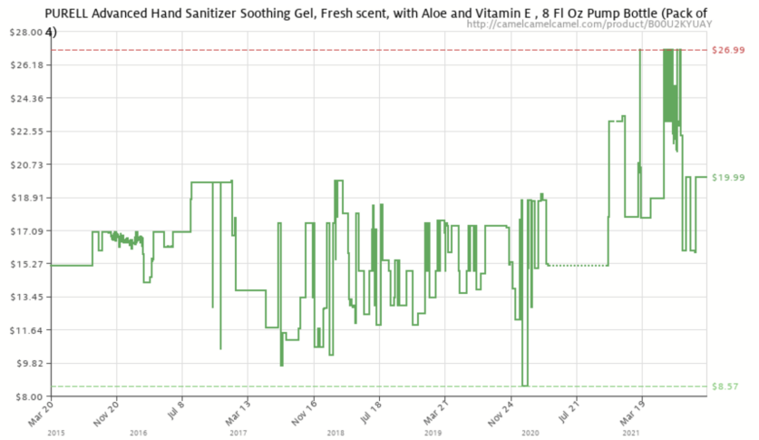
Such issues with increased experimentation are further complicated by the growing litigation and policymaking surrounding algorithmic decisions; e.g., Amazon was recently sued for allegedly price-gouging during the pandemic, as they increased the price of essential goods by more than 450% (e.g., see Figure 1) compared to previously seen prices (McQueen and Ballinger v. Amazon.com). Such misalignment of business practices geared towards profitability, and evolving consumer protection laws (e.g., [9]) raises a natural question for various operational tasks: can firms enforce appropriate fairness desiderata in their online decision-making systems while still achieving good operational performance? In this work, we make two broad contributions to our understanding of this question.

Figure 1: The price path of Purell hand sanitizer on Amazon from March 2015 to March 2021 (from https://camelcamelcamel.com/product/B00U2KYUAY).

• First, we define a general meta-notion of fairness for temporal decision-making called fairness at the time of decision (FTD) to mitigate perceptions of unfairness when an entity receives a decision. In particular, FTD requires that when an entity A receives a decision that affects them at time $t$, comparing this decision to the available data on decisions received by other entities at or before time $t$ must not reveal any problematic disparity in the treatment of entity A. This requirement amounts to a basic prerogative from the perspective of any principal who makes these decisions and is interested in guaranteeing immunity to legal claims of discrimination at the time of the decision. The notion of “problematic disparity" can be modeled by any task-specific notion of fairness for static decision-making, generally requiring that each entity gets a decision that is (approximately) as conducive as that received by others. Thus, FTD adapts to the growing literature on task-specific variants of comparative fairness across a variety of operational applications such as demand learning [10], assortment optimization [11], kidney exchange [12], etc. Importantly, since fairness is not required to be guaranteed from the perspective of an entity after the entity receives the decision, FTD generally allows decisions to become more conducive over time, thus allowing room for (constrained) experimentation and learning.

• Enforcing FTD across time results in a rich class of online optimization problems where decisions must follow a constrained trajectory. This results in the natural question: Is it even possible to ensure FTD in online decisions without sacrificing performance?” As our second contribution, we exemplify the algorithmic challenges in restricting decision trajectories across time in the context of stochastic convex optimization.

  We consider a setup where a principal seeks to optimize real-valued decisions corresponding to $N$ groups of populations. Each group corresponds to an a priori unknown (expected) cost function. We assume that higher decisions are more conducive from the perspective of the groups and we consider a generic comparative notion of fairness that we refer to as envy freeness, which imposes lower bounds on the decision received by each group depending on the decisions received by others. We assume a bandit feedback model where the principal only observes the function value at any decision point corrupted by zero-mean sub-Gaussian noise. This setup can, for example, model a dynamic pricing scenario for multiple customer segments under demand uncertainty, where the firm wants to maximize revenue while satisfying a recently proposed notion of price fairness [10] relative to the past sales data at the time of each purchase (the revenue maximization objective can be equivalently posed as a cost minimization objective).

  Focusing on the case where the cost functions are known to be smooth and strongly convex, we show that significant and non-trivial algorithmic innovations are necessary to satisfy FTD while achieving good regret bounds. A key challenge arises because of bandit feedback since it entails the construction of accurate gradient estimates while satisfying the FTD constraint. In addition, the approach to optimality as the decisions become more conducive must be cautious since if the algorithm overshoots the optimal point, then it cannot backtrack, again due to the FTD constraint. We first design novel approaches to tackle these challenges for the case of two population groups and we show that our algorithms attain a $\widetilde{O}(\sqrt{T})$ regret bound, which is known to be the best achievable without the fairness constraint [13]. We then consider the multi-group case beyond two groups, for which we design a simpler $\widetilde{O}(T^{2/3})$ regret algorithm, although we conjecture that $\widetilde{O}(\sqrt{T})$ regret is achievable using similar ideas as the case of two groups at the cost of a significantly more complex algorithm definition. Our analysis thus illustrates the nature of design tradeoffs that arise in satisfying FTD while ensuring low impact on the utility.

We conclude the paper by discussing various open problems in extending FTD to other practical contexts, open problems arising from related temporal fairness notions, and extensions of FTD. We point to a rich space of exciting problems and research opportunities at the interface of temporal fairness and online optimization.

Organization. The paper is organized as follows. We first discuss related literature in the remainder of this section. In Section 2, we introduce a generic static decision-making scenario and an abstract notion of static fairness whose temporal extensions we will consider. In Section 3 we motivate and introduce the notion of fairness at the time of decision. In Section 4 we define the multi-group stochastic convex optimization problem under bandit feedback and we also introduce the comparative notion of envy freeness. In Section 5, we tackle algorithm design for the case where there are two groups of populations. Our main methodological ideas are developed in this section. Algorithm design for the multi-group case is considered in Section 6. In Section 7, we present numerical experiments validating our approaches using a retail pricing dataset. We finally discuss related problems and extensions in Section 8. The detailed proofs of all our results can be found in the Appendix.

1.1 Related Work

Fairness in static decision-making. Notions of fairness in static decision-making typically ensure that various stakeholders are treated equitably [14]. Two broad varieties of notions have appeared in this regard. First is the popular notion of individual fairness [15], which requires that similar individuals must receive similar treatments. Formally, if $x_{i}$ is the decision received by individual $i$, then individual fairness requires that $|x_{i}-x_{j}|\leq Kd(i,j)$ for any two individuals $i$ and $j$, where $K>0$ is some constant, and $d(i,j)$ is a similarity metric that captures some publicly acceptable notion of “distance" between two individuals that dictates the allowable disparity between their decisions. The second notion is group fairness, also known as statistical parity [16, 17], under which one demands parity in certain statistics of the decisions across multiple groups of people, e.g., requiring that two groups of populations in the same role have similar average salaries in an organization. Such parity notions have been proposed in the context of multi-segment pricing recently by [10] and [18]. For example, the notion of price fairness considered by [10] imposes bounds on the price disparity seen across segments, i.e., they require that $|p_{i}-p_{j}|\leq C_{ij}$ for any two customer segments $i$ and $j$ where $C_{ij}>0$ is some constant. The common aspect of these two notions is that they impose bounds on the degree of envy felt by entities – either individuals or groups – when comparing their decision to others. In Section 2, we consider a generalization of such notions of fairness.

Temporal notions of fairness in dynamic decision-making. Broadly, four different types of temporal notions of fairness have appeared in the literature on online decision-making. The first type of constraint is a time-independent fairness constraint in which a static fairness constraint must be satisfied independently in each period. For example, [19] and [20] consider a multi-segment dynamic pricing problem where the price fairness constraint of [10] must be satisfied in each time period.

In contrast, the second type of fairness constraint is what we refer to as a time-dependent decision-adaptive fairness constraint. FTD is an example of this type of temporal constraint. Such constraint changes depending on the decisions taken in the past, but is agnostic to the outcomes of the decisions. Similar constraints have appeared in recent and parallel literature. For example, [20] requires that the price offered to a particular segment must be close to the prices offered to the same segment over the past $k$ time periods (in addition to satisfying the price fairness constraint across segments every time period). Such a sliding-window fairness constraint was also considered by [21] in the context of adaptive supervised learning.

In a similar vein, and the most related to our paper, [22] define the notion of individual fairness in hindsight in the context of contextual bandit problems. This is a temporal version of the static notion of individual fairness that guarantees individual fairness at the time of decision based on some underlying similarity metric. Our meta-objective of FTD is a significant generalization of this notion that goes beyond individual fairness objectives for static decision-making (e.g., unlike individual fairness, we can model additive as well as multiplicative notions of envy-freeness in our framework, with asymmetric allowable disparities across groups). Moreover, the technical analysis of [22] is restricted to a simple and abstract contextual bandit setup where the decision-maker tries to distinguish between a finite set of utility models. Our framework, on the other hand, allows us to consider a general stochastic convex optimization setup that is applicable in a broader variety of settings.

The third type of temporal fairness constraint is what we refer to as a time-dependent outcome-adaptive fairness constraint, where the constraint can change as the outcomes from the decisions change. For example, [23] has introduced a fairness constraint in a contextual bandit setting requiring that preferential treatment be given to an arriving entity only if it is known with high enough certainty that such preferential treatment is justified by current estimates of the mean rewards resulting from the treatment. Thus, as entities are administered decisions over time, certainty in their reward distributions increases, and they can eventually be treated differently. A Bayesian version of this idea was proposed by [24] in the non-contextual bandit setting, in which decisions are constrained to be fair with respect to the posterior reward distributions of the arms at any time. In this way, as the posterior distributions converge to the true distributions, violations of the desired fairness constraint should diminish. In a similar vein, [25] consider a problem of ensuring group fairness in hiring, where uncertainty is modeled using a partial order and decisions are constrained to be consistent with the partial order at any time.

The fourth type of temporal fairness constraint asks for fairness of certain decision statistics, either ex ante or ex post, across arriving entities over time. For example, [26] considers a sequential resource allocation setting where entities arrive over time with certain demands and the goal is to maximize the minimum fill rate. [27] similarly considers the problem of maximizing the minimum service rate across different groups in an online bipartite matching setting. The main difference from the other three types of constraints is that one doesn’t necessarily seek to guarantee comparative fairness for an entity arriving at a point in time, but rather one guarantees fair treatment of groups of entities across time. A general framework for satisfying such time-average fairness constraints in the context of kidney transplantation has been proposed by [28].

Decision-constrained stochastic convex optimization. Our work makes fundamental contributions to decision-constrained stochastic convex optimization under bandit feedback. In general, none of the existing algorithms from the convex optimization toolkit can be easily modified to satisfy FTD. For example, FTD may require that decisions are monotonically increasing in each dimension as we see in Section 5. Even this requirement cannot be met by simple modifications of existing algorithms. In the noiseless bandit feedback setting, Kiefer gave an $\mathcal{O}(1)$-regret algorithm, now well known as Golden-Section Search, for minimizing a one-dimensional convex function [29]. This algorithm iteratively uses three-point function evaluations to “zoom in” to the optimum, by eliminating a point and sampling a new point in each round. Its mechanics render it infeasible to implement it in a fashion that respects the monotonicity of decisions. For higher dimensions, a $\mathcal{O}(1)$-regret algorithm has been designed by [30]. This algorithm is based on gradient-descent using a one-point gradient estimate constructed by sampling uniformly in a ball around the current point. This key idea recurringly appears in several works on convex optimization with bandit feedback (e.g., [31], [32], [33]). However, due to the randomness in the direction chosen to estimate the gradient, such an approach does not satisfy monotonicity.

For the case of noisy bandit feedback, [13] has shown a lower bound of $\Omega(\sqrt{T})$ in the single-dimensional setting that holds for smooth and strongly convex functions and showed that an appropriately tuned version of the well-known Kiefer-Wolfowitz [34] stochastic approximation algorithm achieves this rate. This algorithm uses two-point function evaluations to construct gradient estimates, which are then utilized to perform gradient-descent. Our near-optimal algorithms in Section 5 are the most related to this approach, where we tackle the significant additional challenge that the two-point evaluations need to consistently satisfy monotonicity over time while attaining the same regret bounds (up to logarithmic factors). For the case of convex functions, Agrawal et al. designed an algorithm that achieves the $\widetilde{\mathcal{O}}(\sqrt{T})$ bound under bandit feedback [35]. In the one-dimensional case, their approach is the most related to the golden-section search procedure of [29], and as such, is infeasible to implement in a monotonic fashion.

Though not motivated by fairness concerns, two recent parallel works have considered the problem of ensuring monotonicity of decisions in stochastic optimization under bandit feedback ([36] and [37]). Assuming that the functions are only known to be Lipschitz and unimodal they find that the optimal achievable regret is $\widetilde{\Theta}(T^{3/4})$, which is higher than the $\widetilde{\Theta}(T^{2/3})$ regret achievable without the monotonicity requirement. In contrast, Theorem 2 implies that under the assumption that the cost functions are smooth and strongly convex, the unconstrained optimal regret bound of $\widetilde{\mathcal{O}}(\sqrt{T})$ is attainable while ensuring monotonicity of decisions (up to logarithmic terms). We also note that, because the settings considered by these other works are more pessimistic in their view of the possible cost functions, algorithm-design for optimizing the worst-case turns out to be simpler. In particular, both [36] and [37] show that we cannot do better than the simple approach of sequentially traversing the decision space in a fixed direction and using a fixed step size until the utility keeps increasing (as determined by a sequence of two-point hypothesis tests). In contrast, the problem of leveraging gradient information while maintaining monotonicity, while also ensuring negligible impact on regret, results in several novel and non-trivial aspects of our algorithm design.

2 Fairness in static decision-making

Consider a static decision-making scenario, where there is a finite set $\mathcal{I}=\{1,\cdots,N\}$ of entities representing the stakeholders receiving the decisions. For example, an entity could represent a customer segment (such as “youth”) in a pricing scenario or a job applicant in an applicant-screening scenario. The decisions lie in the set $\mathcal{X}$ (e.g., the range of prices that can be offered to a customer, or accept/reject decisions for screening). There is a principal (such as a firm or a platform) who chooses a decision rule that maps entities to decisions. We represent such a rule by the vector $\mathbf{x}=(x(1),\cdots,x(N))$, where $x(i)\in\mathcal{X}$ is the decision assigned to entity $i$. There is an evaluator function $\mathcal{U}$ that measures the utility from a decision rule, which represents some operational performance measure such as social welfare, efficiency, principal utility, etc.

The decision rule is required to satisfy a task-specific notion of comparative fairness. Such a notion typically imposes certain entity-specific equity constraints, which ensure that each entity is treated equitably when compared to others. Consider the following two examples from recent literature.

1. Fair pricing. Consider a product pricing scenario with $N$ customer segments. Let $x(i)$ be the price offered to segment $i$. To ensure comparative fairness from the perspective of segment $i$, we may require certain upper bounds on the price offered to $i$ depending on the prices offered to the other segments. For instance, we may require that $x(i)\leq x(i^{\prime})+s(i,i^{\prime})$, where $s(i,i^{\prime})\in\mathbb{R}$ represents a permissible additive slack that depends on the two segments in comparison; e.g., if the two segments are youth (1) and adults (2), we may require that $x(1)\leq x(2)$, i.e., the price offered to the youth segment must be at most that offered to the adults. Similarly, we may require that $x(2)\leq x(1)+5$, i.e., while the adults can be priced higher than the youth, the difference cannot be larger than $$5$. Such a notion of price fairness has been recently proposed by [10] under the assumption that the slacks are non-negative and symmetric (so that the constraints amount to requiring that $|x(i)-x(i^{\prime})|\leq s(i,i^{\prime})=s(i^{\prime},i)$ for all segments $i,\,i^{\prime}$). We will consider such a notion of comparative fairness in the context of stochastic convex optimization in Section 4.1.

2. Fair assortment planning. [11] consider a platform making an assortment planning decision from amongst $N$ products/sellers to show to a customer. Each product $i$ has some weight $w_{i}\geq 0$ that measures how popular the product is to customers; in particular, upon offering the customers an assortment $\mathcal{S}$ of products, the customers purchase product $i\in\mathcal{S}$ according to the Multinomial Logit Choice (MNL) model, with probability $w_{i}/(1+w(\mathcal{S}))$ where $w(\mathcal{S})=\sum_{j\in\mathcal{S}}w_{j}$. Given a probabilistic assortment choice of the platform, suppose that $x(i)$ is the probability that $i$ is included in the assortment, referred to as the visibility offered to product $i$. [11] propose a notion of fairness that requires that for every product $i$ and for some $\delta>0$,

   $$x(i)\geq\frac{w_{i^{\prime}}}{w_{i}}x(i^{\prime})-\delta,$$

   for all $i^{\prime}$. That is, $i$ must get at least as much visibility (with a $\delta$ slack) as $i^{\prime}$ after adjusting for their relative differences in popularities, for every $i^{\prime}$.

To generally capture such comparative notions of fairness exemplified by these settings, let’s suppose that for each entity $i\in\mathcal{I}$, there exists a set of $K_{i}$ real-valued functions, $F_{i,j}:\mathcal{X}\times\mathcal{X}^{N}\rightarrow\mathbb{R}$, for $j\in[K_{i}]$, each of which maps (a) the decision received by entity $i$, and (b) the profile of decisions $\mathbf{x}$ received by all the entities, to a real number. We then assume that the fairness notion requires that

$$F_{i,j}(x(i),\mathbf{x})\leq 0\textrm{ for all }i\in\mathcal{I}\textrm{ and }j\in[K_{i}].$$ (1)

For example, $F_{i,j}(x(i),\mathbf{x}):=0.9~{}(\max_{s\in[N]}x(s))-x_{i}$ imposes a constraint that decision of $i$th entity is at least 0.9 times the maximum decision received by any other entity. The idea is that the $K_{i}$ entity-specific constraints capture the fairness requirements from the perspective of entity $i$ on comparing its decision with the decision profile across all entities. We include the decision for entity $i$ twice in the argument of $F_{i,j}$ because later when we incorporate time, we may want to compare the decision received by entity $i$ at time $t$ against that received at some other time $t^{\prime}$.

The static optimization problem of maximizing the utility of a decision rule subject to fairness constraints can then be expressed as follows.

$$\text{maximize}\,\,\,\mathcal{U}(\mathbf{x})$$ (2)

subject to $$F_{i,j}(x(i),\mathbf{x})\leq 0\textrm{ for all }i\in\mathcal{I}\textrm{ and }j\in[K_{i}].$$ (3)

When $\mathcal{U}$ and $F_{i,j}$ are well-behaved functions, one can find a solution using standard optimization techniques.

3 Fairness at the time of decision in dynamic decision-making

The introduction of time in the above setup makes it more interesting. Suppose that the principal chooses decision rules over a time horizon of multiple periods, $t\in\{1,\ldots,T\}=[T]$. Let’s denote the decision rule at time $t$ as $\mathbf{x}_{t}\in\mathcal{X}^{N}$. First, note that if there is no reason to choose different decision rules across time periods, e.g., in settings where the utility function $\mathcal{U}$ is unchanging and known to the principal, then the time dimension is redundant since the principal can simply choose the same static-optimal fair decision rule at each time. However, if (a) $\mathcal{U}$ is unknown to the principal and the optimal fair decision rule must be learned over time, or (b) if $\mathcal{U}$ is known but it changes over time, then the ability to change decision rules may be fundamental to attaining good utility. Thus a temporal fairness constraint should ideally allow room for some changes in decisions over time. At the same time, it should satisfy a meaningful desideratum of equity and non-discrimination from the perspective of the entities. We now present our main proposal in this regard.

Definition 1 (Fairness at the time of decision (FTD)).

Consider a static notion of fairness captured by the functions $F_{i,j}$ for $i\in\mathcal{I}$ and $j\in[K_{i}]$. A sequence of decision rules $(\mathbf{x}_{t})_{t\in\mathbb{N},\,t\leq T}$ satisfies fairness at the time of decision if for all $i\in\mathcal{I}$,

$$F_{i,j}\left(x_{t}(i),\left(x_{t_{1}}(1),\cdots,x_{t_{N}}(N)\right)\right)\leq 0\textrm{ for all }j\in[K_{i}],\,\,t\in[T],\textrm{ and }(t_{1},\cdots,t_{N})\in[t]^{N}.$$ (4)

FTD requires that the fairness constraints from the perspective of entity $i$ at time $t$ are satisfied not only with respect to the decisions received by others at time $t$, but also with respect to decisions that were received at any time in the past. For example, consider salary administration in an organization where a non-discrimination requirement dictates that women’s average salary for a role must be at least as much as men’s and vice versa (effectively implying that their average salaries should be equal). FTD in such a scenario would require that women’s average salary in the year 2022 must be at least as high as that of men in 2020 (or any year $\leq$ 2022), but men’s average salary in 2020 need not be as high as that of women in 2022. This effectively means that while the average salary of men and women must be identical within a year, it can increase over years. The attractive feature of this definition is that, when the salaries are decided in a year, both the groups are revealed to be treated fairly with respect to all of the past salary data: they get at least as much pay as that received by anyone in the past. However, the salaries may increase further in the later years, leading to the current salary decisions turning out to be unfair in retrospect in light of the future data.

To further appreciate the notion of FTD, we contrast it against other natural temporal extension of static fairness. The first and most basic possibility in this regard is to simply ignore the temporal aspect and ensure that the static fairness constraints are satisfied for each group independently in each time period. That is, we require that $F_{i,j}\left(x_{t}(i),\mathbf{x}_{t}\right)\leq 0$ for all $j\in[K_{i}]$, $i\in\mathcal{I}$, and across all times $t\in[T]$. This allows for decisions to change arbitrarily between time periods and hence is typically insufficient as a notion of fairness, e.g., it may be difficult to justify that the price of a smartphone seen by a particular customer segment is higher than that seen by the same segment the day before for no apparent reason.

The second possibility lies on the opposite end of the spectrum, requiring that the fairness of a decision must be satisfied with respect to decisions across all times. That is for each $i\in\mathcal{I}$,

$$F_{i,j}\left(x_{t}(i),\left(x_{t_{1}}(1),\cdots,x_{t_{N}}(N)\right)\right)\leq 0\textrm{ for all }j\in[K_{i}]\textrm{ and for all }(t,t_{1},\cdots,t_{N})\in[T]^{N+1}.$$ (5)

While ideal from a fairness perspective, this requirement is too stringent since it often disallows any change in decisions over time [22]. For instance, in the context of salary administration, this requirement means that women’s average salary in the year 2022 must be at least as high as that of men in 2020 and vice versa, effectively implying that the average salaries of men and women must be the same fixed value across all time.

Fairness at the time of the decision thus occupies a convenient middle ground that straddles the extremes of temporal notions of fairness discussed above. As we will see in the next section, FTD leads to technically new challenges in online optimization: it offers enough flexibility in decisions that could potentially allow for some experimentation and learning, and at the same time these intertemporal constraints are novel in the context of online optimization and require new design tools and techniques to assimilate them while ensuring good utility guarantees.

4 Application to multi-group stochastic convex optimization with bandit feedback

We now consider algorithm design for satisfying FTD within the framework of stochastic convex optimization under bandit feedback. We consider the setup of a principal that administers decisions to a finite set $\mathcal{I}=\{1,\cdots,N\}$ of population groups over a horizon of $T$ periods. Decisions lie in the set $\mathcal{X}=[x_{\min},x_{\max}]\subseteq\mathbb{R}^{\geq 0}$ for each group. We further assume that there is a directionality in the conduciveness of decisions from the perspective of the groups, and without loss of generality, we assume that higher decisions are perceived to be better by any group (e.g., a higher salary). Each group $i$ is also associated with a cost function $f_{i}$ (or equivalently a utility function $-f_{i}$) that captures the utility to the principal. In terms of our earlier notation, the goal of the principal is to maximize $\mathcal{U}(\mathbf{x})=\sum_{i\in\mathcal{I}}-f_{i}(x_{i})$. The setup can, for example, model a firm setting prices for $N$ customer segments with revenue function $\textup{Rev}_{i}$ corresponding to group $i$ (one can define $f_{i}=-\textup{Rev}_{i}$), where the prices lie in some set $\mathcal{P}=[p_{\min},p_{\max}]\subseteq\mathbb{R}^{\geq 0}$. In this scenario, a lower price is perceived to be better by any customer.

If these cost functions are known to the principal, and if there are no additional constraints on the decisions, then the principal can simply choose the optimal decision of $x^{*}_{i}\in\operatorname*{arg\,min}_{x\in\mathcal{X}}f_{i}(p)$ for each segment $i\in\mathcal{I}$. We next define the static optimization problem of choosing decisions to minimize cost while satisfying certain comparative fairness constraints.

4.1 Static optimization under envy-freeness

We will consider a static fairness notion of envy freeness while allowing for certain additive disparities. Envy freeness is a commonly studied notion of fairness in the literature on social choice and fair division of resources, which requires that an entity should not envy an allocation received by someone else, i.e., prefer someone else’s allocation over their own allocation [39, 40, 41]. In our setting, since higher decisions are perceived to be better by any group, each group will envy every group that receives a higher decision. Thus, to eliminate envy is to ensure equal decisions across groups. However, instead of eliminating envy, we consider a generalization that allows for certain limits on the envy between any two groups. In particular, we define the “slack” functions defined on ordered pairs of groups: $s(\cdot,\cdot):\mathcal{I}\times\mathcal{I}\rightarrow\mathbb{R}^{\geq 0}$, where we assume that $s(i,i)=0$ for all $i\in\mathcal{I}$. Consider then the following definition.

Definition 2 (Envy Freeness with Additive Slacks).

We say that a decision vector $\mathbf{x}\in\mathcal{X}^{N}$ satisfies envy-freeness (EF) with additive slacks if the following inequalities hold:

$$x_{i}\geq x_{j}-s(i,j)\textrm{ for all }i,j\in\mathcal{I}.$$ (6)

Despite the existence of slacks, we will refer to this notion as envy freeness (EF) for convenience. These constraints say that, e.g., group $i$ should not receive a decision that is much lower than group $j$, with the slack $s(i,j)$ specifying how much difference is permissible. The slack need not be symmetric, i.e., $s(i,j)$ may not necessarily equal $s(j,i)$. In the pricing example, since lower decisions are more conducive, if $p_{i}$ is the price received by group $i$, then the corresponding constraint would be that $p_{i}\leq p_{j}+s(i,j)\textrm{ for all }i,j\in\mathcal{I}$. (Note that the direction of this constraint does not matter from an algorithmic perspective: our algorithms can be trivially modified to temporally satisfy the EF constraint in any fixed direction.) As noted earlier, EF in the context of pricing thus generalizes the price fairness proposal of [20], in which the slack functions are assumed to be symmetric.

Note that the constraints eq. 6 are always feasible since the principal can make the same decision for each group. These constraints are also linear and hence, convex. Let the set of decision vectors in $\mathcal{X}^{N}$ satisfying the EF constraints in eq. 6 be denoted as $\mathcal{X}^{N}_{F}\subseteq\mathcal{X}^{N}$. Then the problem of cost minimization under the EF constraints is defined as

$$C^{*}_{F}=\min_{\mathbf{x}\in\mathcal{X}^{N}_{F}}\sum_{i\in\mathcal{I}}f_{i}(x_{i}).$$ (7)

Assuming that $f_{i}$ are well-behaved, e.g., convex, the set of optimal fair decisions can be easily computed if these $f_{i}$ are known. The challenge is in ensuring temporal fairness constraints when $f_{i}$ are unknown and must be learned over time.

4.2 Ensuring Envy Freeness at the time of decision in multi-group stochastic convex optimization with bandit feedback

We now formulate the problem of stochastic convex optimization with bandit feedback under the constraint of ensuring envy freeness at the time of decision. Consider the setting where the cost functions $f_{i}$ are unknown to the principal. The principal hopes to learn to administer the solution to (7) under the temporal fairness constraint over a discrete time horizon $T$. We make the following assumptions on the cost functions $f_{i}$.

Assumption 1.

We assume that for all $i\in\mathcal{I}$, the function $f_{i}$ is

1. $\alpha$-strongly convex, i.e., $f_{i}(y)\geq f_{i}(x)+\nabla f_{i}(x)(y-x)+\frac{\alpha}{2}(y-x)^{2}$ for all $x,y\in\mathcal{X}$, and

2. $\beta$-smooth, i.e., $f_{i}(y)\leq f_{i}(x)+\nabla f_{i}(x)(y-x)+\frac{\beta}{2}(y-x)^{2}$ for all $x,y\in\mathcal{X}$,

for some $\alpha>$ and $\beta>0$ known to the principal.

These assumptions are commonly made in the convex optimization literature and they allow us to focus on the difficulties that arise in adapting gradient-driven online optimization procedures to satisfy the FTD constraint. In the context of pricing, the corresponding assumption is that the revenue functions are strongly concave and smooth. This assumption is satisfied under the popular linear demand model that is commonly assumed in the pricing literature [42, 43]. Even beyond linear demand models, we argue in Appendix D that this may be a reasonable assumption in many dynamic pricing scenarios where the firm has past sales data on similar products.

Envy freeness at the time of decision (EFTD). Given the notion of envy freeness for static decision-making, the notion of FTD amounts to the following temporal fairness notion.

Definition 3.

A sequence of decisions is said to satisfy envy freeness at the time of the decision (EFTD) if

$$x_{i,t}\geq x_{j,t^{\prime}}-s(i,j)\textrm{ for all }i,\,j\in\mathcal{I},\textrm{ and }1\leq t^{\prime}\leq t\leq T.$$ (8)

The idea is that the decisions received at at time $t$ need to satisfy the EF only relative to the decisions administered at times $t^{\prime}\leq t$.

Dynamics and feedback. At each time period $t$, the algorithm produces a decision $\mathbf{x}_{t}\in\mathcal{X}^{N}$ and observes bandit feedback, i.e., the function values for each $i$ at the chosen decision $x_{i,t}$ potentially corrupted with noise. In particular, we assume that the feedback observed is a random variable $Y_{i,t}=f_{i}(x_{i,t})+\varepsilon_{i,t}$, where $(\varepsilon_{i,t})_{1\leq t\leq T}$ for each $i\in\mathcal{I}$ is a sequence of random variables representing the noise in the feedback. Note that the distribution of $\varepsilon_{i,t}$ can potentially depend on $x_{i,t}$. We make the following commonly made assumption on this sequence.

Assumption 2.

For each $i$, and a sequence of decisions $x_{i,1},\ldots,x_{i,T}$, the random variables $\varepsilon_{i,1},\ldots,\varepsilon_{i,T}$ are independent, have zero mean, and are sub-Gaussian: there exists a constant $c>0$ such that $\mathbb{P}(|\varepsilon_{i,t}|\geq s)\leq 2e^{-cs^{2}}$ for all $s$. We also assume that they have bounded norm $\max_{i,t}\|\varepsilon_{i,t}\|_{\psi_{2}}\leq E_{\max}$, where $\|\varepsilon_{i,t}\|_{\psi_{2}}=\inf\big{\{}s>0:\mathbb{E}[\exp(\varepsilon_{i,t}^{2}/s^{2})]\leq 2\big{\}}$.

Objective and constraints. The problem is an online decision-making problem, in that the decision $\mathbf{x}_{t}$ at time $t$ is made using the historic information $\mathcal{H}_{t-1}=\left(\mathbf{x}_{1},\mathbf{Y}_{1},\ldots,\mathbf{x}_{t-1},\mathbf{Y}_{t-1}\right)$. These decisions are further constrained to respect the EFTD constraint: $x_{i,t}\geq x_{j,t^{\prime}}-s(i,j)\textrm{ for all }i,\,j\in\mathcal{I},\textrm{ and }1\leq t^{\prime}\leq t\leq T$. The regret incurred by an algorithm is defined to be

$$\sum_{t=1}^{T}\sum_{i\in\mathcal{I}}E(f_{i}(x_{i,t}))-T\min_{\mathbf{x}\in\mathcal{X}^{N}_{F}}\sum_{i\in\mathcal{I}}f_{i}(x_{i}),$$ (9)

where the expectation is over the randomness in $(\mathbf{x}_{t})_{1\leq t\leq T}$, and where recall that $\mathcal{X}^{N}_{F}$ denotes the set of decision vectors $\mathbf{x}$ that satisfy the EF constraint.

Our objective is to design an algorithm that minimizes regret in the worst case over all $\alpha$-strongly convex and $\beta$-smooth functions while ensuring that the decisions satisfy the EFTD constraint. We say that an algorithm is a $P$-regret algorithm if its regret is at most $P$.

5 A near-optimal EFTD algorithm with two groups

Ensuring EFTD imposes complex constraints across decisions over time. In this section, we tackle the challenges that arise in designing a near-optimal regret algorithm for the simplest case of two population groups. First, let’s examine what the EFTD constraints require in this setting. These constraints can be broken down into two parts:

1. Coordinate-wise monotonicity. We first require that $x_{i,t}\geq x_{i,t^{\prime}}$ for $1\leq t^{\prime}\leq t\leq T$ and for $i=1,2$, which means that the decisions on each coordinate must (weakly) increase over time.

2. Cross-coordinate constraints. We also have that $x_{1,t}\geq x_{2,t^{\prime}}-s(1,2)$ and $x_{2,t}\geq x_{1,t^{\prime}}-s(2,1)$ for all $1\leq t^{\prime}\leq t\leq T$, which means that the decision for group $i$ at any time can be at most $s(i,-i)$ less than the highest decision seen by group $-i$ so far.

Because several ideas will be necessary for designing a near-optimal regret algorithm that satisfies these constraints with just bandit feedback, we break down this problem into parts. First, we will consider a single-group online stochastic optimization problem where the only constraint is to satisfy weak monotonicity. The algorithmic approach we develop for that case will then be used as a component in the two-group case where we additionally have to tackle the cross-coordinate constraints.

5.1 Single group monotonic stochastic optimization with bandit feedback.

In this section, we consider the problem of minimizing a smooth and strongly convex function $f(\cdot)$ over the feasible set $\mathcal{X}$ under noisy bandit feedback, while ensuring that the decisions monotonically (weakly) increase over time and while ensuring low regret. We denote $x^{*}=\operatorname*{arg\,max}_{x\in\mathcal{X}}f(x)$. As we noted earlier in Section 1.1, none of the existing stochastic optimization algorithms designed for this setting satisfy monotonicity.

Algorithmic approach. At their core, our algorithm relies on gradient estimates constructed from monotonic two-point function evaluations (i.e., “secant” information) to improve decisions as in the well-known Keifer-Wolfowitz algorithm for convex optimization with noisy bandit feedback [34]. Due to the monotonicity constraint, the challenge is to ensure that sufficient progress is continually made towards reaching the optimal decision using gradient information while avoiding excessively overshooting the optimum (since backtracking is disallowed). There are two key algorithmic ideas we develop to tackle this challenge: (a) taking gradient steps from a “lagged" point to avoid overshooting the optimum, and (b) adapting the lag size to local gradient estimates to tailor the degree of caution to the distance from the optimum point, while ensuring monotonicity.

Warm-up: the case of noiseless bandit feedback. We first consider algorithm design in the noiseless bandit setting: a decision $x_{t}\in\mathcal{X}$ is made at each time $t\in[T]$, and for each decision $x_{t}$, the algorithm observes $f(x_{t})$. The decisions made by the algorithm are constrained to be monotone: $x_{1}\leq x_{2}\leq\cdots\leq x_{T}$.

input : strong convexity parameter $\alpha$, smoothness parameter $\beta$, time horizon $T$, $\mathcal{X}=[x_{\min},x_{\max}]$

1 Set $x_{1}^{\prime}\leftarrow x_{\min}$ and $x_{1}\leftarrow x_{1}^{\prime}+\delta$, and observe $f(x_{1}^{\prime})$ and $f(x_{1})$

2 for $t=1,\ldots,T/2$ do

3        Let $\widetilde{\nabla}_{t}\leftarrow\frac{f(x_{t})-f(x_{t}^{\prime})}{x_{t}-x_{t}^{\prime}}$

4        if $-\frac{1}{\beta}\widetilde{\nabla}_{t}\geq(1+\gamma)\delta$ then

5               Sample $f(\cdot)$ at $x_{t+1}^{\prime}=x_{t}^{\prime}-\frac{1}{\beta}\widetilde{\nabla}_{t}-\delta_{t+1}$ (lagged iterate)

6               Sample $f(\cdot)$ at $x_{(t+1)}=x_{t+1}^{\prime}+\delta_{t+1}$ (non-lagged iterate)

7        else

8               Exit from loop and stabilize at $x_{t}$

9              

10       

Algorithm 1 Lagged Gradient Descent (Lgd) (noiseless bandit)

We present a monotonic procedure called Lagged Gradient Descent (Lgd) (Algorithm 1) for this setting, which is a variation on classical gradient descent. At each round, we use two queries (one at $x_{t}$ and one at the “lagged” point $x_{t}^{\prime}=x_{t}-\delta$) to estimate the gradient. Since we need to ensure monotonicity of iterates, we need to sample first at the lagged point $x_{t}^{\prime}$ and next at $x_{t}$ to get an estimate of the gradient. The size of $\delta$ will depend on the time horizon $T$ and be optimized for minimizing the regret of the overall scheme. We then move by an amount proportional to the estimated gradient.

While increasing decisions, even in this non-noisy case, we need to be careful about not excessively overshooting the optimum point, which could result in high regret due to the monotonicity constraint that disallows backtracking. To avoid overshooting, we move proportional to the gradient from the lagged point $x_{t}^{\prime}$ instead of from $x_{t}$. Since the estimated gradient $\widetilde{\nabla}_{t}$ in Lagged Gradient Descent is less steep than the true gradient at $x_{t}^{\prime}$, the smoothness of $f$ allows us to ensure that we never overshoot. However, since we jump from $x_{t}^{\prime}$ instead of $x_{t}$, a small jump (of a magnitude smaller than $|x_{t}-x^{\prime}_{t}|$) may violate monotonicity. To avoid this, we jump forward only if the gradient is steep enough; in particular, if the magnitude of the estimated gradient is at least $\beta(1+\gamma)\delta$, for some $\gamma>1$, defined in Theorem 1.

Lemma 1 below shows that the decisions resulting from Lagged Gradient Descent (Lgd) are monotonic, they avoid overshooting, and their convergence rate to the optimum is exponential.

Lemma 1.

Let $f:\mathcal{X}\to\mathbf{R}$ be an $\alpha$-strongly convex and $\beta$-smooth function. Let $x_{1},\ldots,x_{T/2}$ be the non-lagged points generated by Lagged Gradient Descent (Algorithm 1), and assume that $x_{1}\leq x^{*}=\arg\,\min_{x\in\mathbb{R}}f(x)$. Then, for $\gamma>1$, the following hold:

1. Decisions increase monotonically toward the optimum: $x_{1}\leq x_{2}\leq x_{3}\leq\cdots\leq x_{T/2}\leq x^{*}$;

2. The convergence rate is exponential up to halting: $h_{t+1}\leq h_{1}\exp\big{(}-2\alpha ct\big{)}$, where $h_{t}=|x_{t}-x^{*}|$ and $c=\frac{1}{2\beta}-\frac{1}{(1+\gamma)\beta}$.

With this convergence rate established, we can calculate a regret bound for Lgd. We can break the regret of this procedure into three categories: regret during exploration, regret due to stopping (i.e., regret incurred after the “for loop” has ended), and regret due to potential overshooting (which is 0 by Lemma 1). We balance these three to obtain an $\mathcal{O}(1)$ regret bound.

Theorem 1.

Assume that $x^{*}=\arg\,\min_{x\in\mathbf{R}}f(x)\in(x_{\min},x_{\max}]$, and fix $\delta=T^{-1/2}$ and $\gamma=1+\frac{1}{\log T}$. Then Lagged Gradient Descent (Alg. 1) is a $\mathcal{O}(1)$-regret EFTD algorithm for optimizing an $\alpha$-smooth and $\beta$-strongly convex function in the noiseless bandit setting.

Theorem 1 shows that imposing monotonicity has no (asymptotic) effect on the hardness of the noiseless setting: a non-monotonic constant-regret procedure is already known [29], and Lgd is a monotonic constant-regret procedure.

One important aspect of the noiseless setting is that gradient estimation is easy: one simply requires two samples, and additionally, the gap $\delta$ between the samples can be arbitrarily small, resulting in arbitrarily accurate gradients. As we will discuss in the next section, when noise is introduced, there is a trade-off between the magnitude of $\delta$ and the number of samples required to accurately estimate the gradient. This tension ultimately results in a higher regret bound.

input : convexity parameters $\alpha$, $\beta$, time horizon $T$, feasible set $\mathcal{X}=[x_{\min},x_{\max}]$, initial lag size $\delta_{1}$, stopping parameter $\gamma>1$, $q\in(0,1)$, noise sub-Gaussian norm bound $E_{\max}$, Hoeffding constant $C$

1 $\delta_{i}\leftarrow q^{i-1}\delta_{1}$ for $i\geq 2$, $\xi\leftarrow 1-q$, $n(d)=\frac{64E_{\max}^{2}\log\frac{2}{p}}{C\alpha^{2}d^{4}}$ for any $d$, $x_{1}\leftarrow x_{\min}+\delta_{1}$, $t\leftarrow 1$, $i\leftarrow 0$

2 repeat

3        $i\leftarrow i-1$

4        repeat

5               $i\leftarrow i+1$

6               $\overline{f}(x_{t}-\delta_{i})\leftarrow$ average of $n(\xi\delta_{i})$ samples at $x_{t}-\delta_{i}$ // estimate $f(x_{t}-\delta_{i})$

7               $\overline{f}(x_{t}-\delta_{i+1})\leftarrow$ average of $n(\xi\delta_{i})$ samples at $x_{t}-\delta_{i+1}$ // estimate $f(x_{t}-\delta_{i+1})$

8               $g_{t}^{(i)}\leftarrow\frac{\overline{f}(x_{t}-\delta_{i+1})-\overline{f}(x_{t}-\delta_{i})+\alpha\xi^{2}\delta_{i}^{2}/4}{\xi\delta_{i}}$ // compute the approximate secant

9              

10       until $-\frac{1}{\beta}g_{t}^{(i)}\geq(2+\gamma)\delta_{i}$

11       $\overline{f}(x_{t})\leftarrow$ average of $n(\delta_{i})$ samples at $x_{t}$ // estimate $f(x_{t})$

12        $\widetilde{\widetilde{\nabla}}_{t}\leftarrow\frac{\overline{f}(x_{t})-\overline{f}(x_{t}-\delta_{i})+\alpha\delta_{i}^{2}/4}{\delta_{i}}$ // compute the approximate secant

13        Compute $x_{t+1}\leftarrow x_{t}-\frac{1}{\beta}\widetilde{\widetilde{\nabla}}_{t}-\delta_{i}$

14        if $x_{t+1}>x_{\max}$ then

15               Set $x_{s}\leftarrow x_{\max}$ for all $t+1\leq s\leq T$

16       $t\leftarrow t+1$

17       

18until $T$ samples have been taken

Algorithm 2 Adaptive Lagged Gradient Descent (Ada-Lgd)

The challenges posed by noisy bandit feedback. Recall that in the noisy bandit setting, upon querying the $t^{\textup{th}}$ point $x_{t}$, the algorithm observes $f(x_{t})+\varepsilon_{t}$, where the noise $\varepsilon_{t}$ is assumed to be independent, mean zero, and sub-Gaussian of bounded sub-Gaussian norm (Assumption 2). To appreciate the complication added by the noise, let’s suppose we try to replicate the approach in Lagged Gradient Descent, in which we utilize secant calculations with a fixed lag size $\delta$ to estimate the gradient step. In the absence of noise, the secant is always sandwiched between the true gradients at $x_{t}$ and the lagged point $x_{t}-\delta$ by the mean value theorem. Thus moving from the lagged point using the secant ensures that the algorithm never overshoots the optimum. But when the function evaluations are noisy, multiple function evaluations are necessary to evaluate the secant accurately enough for this sandwich property to hold. In particular, one can show that $\Theta(1/\delta^{4})$ function evaluations are necessary at the two points to get such an accurate secant estimate (Lemma 4 in the appendix). So, if one uses $\delta=T^{-1/2}$ as in the analysis of noiseless Lgd (Theorem 1), the number of samples required at each point is $\Omega(T^{2})$. Such high sampling rates may be acceptable when the algorithm iterates are very close to the optimum, but will lead to a high (linear) regret when the iterates are farther from the optimum. Thus, clearly, $\delta$ cannot be set to be that small.

At the same time if $\delta$ is too large then the algorithm may stop far from the optimum, since the local gradient may prematurely become small enough relative to the lag size that jumping from a lagged point may violate monotonicity (i.e., the condition $-\frac{1}{\beta}g<(1+\gamma)\delta$ is satisfied). Such premature stopping will again cause high regret. Later in Section 6, we will see that one can set a fixed $\delta$ that optimizes this tradeoff and obtain a regret of $\widetilde{\mathcal{O}}(T^{2/3})$ in the multi-group setting.

However, it turns out that we can do strictly better and obtain the near-optimal regret rate of $\widetilde{\mathcal{O}}(\sqrt{T})$ by choosing the lag sizes adaptively. The key idea is that if the algorithm stops moving with a particular lag size $\delta$, then we reduce the lag size so that the algorithm can continue to proceed. This ensures that smaller lag sizes and correspondingly higher sampling rates are utilized only when the iterates are closer to the optimum when they do not result in high regret.

This approach, however, presents a crucial challenge: when estimating the secant at a point $x_{t}$ and a lagged point $x_{t}-\delta$, the decision of whether the lag size must be reduced from $\delta$ to some smaller quantity must be made before we sample at $x_{t}$ to insure monotonicity of the iterates. To address this challenge, we design a novel algorithm that respects monotonicity while searching for the correct lag size.

Adaptive Lagged Gradient Descent. We develop a novel procedure called Adaptive Lagged Gradient Descent (Ada-Lgd) (Alg. 2) in this section. In this procedure, there are “non-lagged” iterates, denoted as $(x_{t})_{t\in\mathbb{N}}$, and “lagged” iterates denoted in relation to the non-lagged iterates, e.g., $x_{t}-\delta_{i}$ for some specified $i$. For any non-lagged iterate $x_{t}$ such that $x_{t+1}=x_{t}-\frac{1}{\beta}\widetilde{\widetilde{\nabla}}_{t}-\delta_{i}$, we say that $\delta_{i}$ is the lag size of $x_{t}$.

We now describe how Ada-Lgd reduces the lag sizes in a monotonic manner. Suppose the current lag size is $\delta_{i}$, and we are sampling at $x_{t}-\delta_{i}$. Right after sampling at $x_{t}-\delta_{i}$, we sample at $x_{t}-\delta_{i+1}$ (where $\delta_{i+1}=q\delta_{i}$ for some $q<1$). This has the benefit of providing a gradient estimate at $x_{t}-\delta_{i}$. This estimate in turn gives us an estimate of the gradient at $x_{t}$, which can be used in deciding whether or not the lag size should indeed be reduced to $\delta_{i+1}$ or lower. If yes, then we continue to sample at $x_{t}-\delta_{i+2}$ and continue the search for the right lag size; else, we finally sample at $x_{t}$ and continue the secant descent procedure. Such pre-emptive sampling to search for the correct lag size thus guarantees monotonicity.

Figure 2: Illustration of the points: the algorithm starts exploring at $p_{\min}=x_{1}-\delta_{1}$ followed by $x_{1}-\delta_{2}$. In this case, Phase 1 consists of $x_{1}$, Phase 2 consists of $x_{2}$ and $x_{3}$, Phase 3 consists of $x_{4}$, and Phase 4 consists of $x_{5}$; the step-size indices are $n_{1}=2,n_{2}=5,n_{3}=8$, and $n_{4}=9$. The computation of $x_{t+1}$ is given by approximate gradient from the chosen lagged point, as depicted by the dotted lines, using the estimate $\widetilde{\widetilde{\nabla}}_{t}(x_{t}-\delta_{i},x_{t})$ obtained by sampling at $x_{t}-\delta_{i}$ and $x_{t}$.

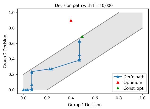
In view of these dynamics, it is useful to think of the iterates with the same lag size as forming a phase, where phases are numbered chronologically: Phase 1 is the phase containing $x_{1}$, Phase 2 is the next phase, and so on. The lag size associated to Phase $j$ is denoted $\delta_{n_{j}}$. Since multiple lag sizes can be skipped between $x_{t}$ and $x_{t+1}$, it may be the case that $n_{i+1}>n_{i}+1$. For example, see Figure 2, where the first jump is taken with a lag size of $\delta_{2}=q\delta_{1}$. While sampling at $x_{2}-\delta_{2}$ and $x_{2}-\delta_{3}$, since the estimated gradient is not steep enough, the algorithm begins sampling at $x_{2}-\delta_{4}$. The algorithm decreases the lag size twice more before deciding that $\delta_{5}$ is an appropriate lag size. In this case, $x_{2}-\delta_{5}$ is the “chosen” lagged point. Theorem 2 formalizes the regret guarantee achieved:

Theorem 2.

Assume that $x^{*}=\arg\,\min_{x\in\mathbb{R}}f(x)\in(x_{\min},x_{\max}]$, and assume the noise is mean zero, independent, and sub-Gaussian of bounded sub-Gaussian norm (Assumption 2). Then Ada-Lgd (Algorithm 2) satisfies EFTD and, on input of $\delta_{1}=1/\log T$, $\gamma=1+\frac{1}{\log T}$, any $q\in(0,1)$, and $p=T^{-2}$, incurs regret of order $\mathcal{O}\left((\log T)^{2}T^{1/2}\right)$.

There are several steps in the proof of Theorem 2, which is presented in Appendix A.2. We first show that all the secant estimates are accurate enough with high probability so that the sandwich property holds, i.e., the secant is indeed sandwiched between the gradients at the two points (Claim 3 in the proof). With this established, we show that overshooting does not occur (Claim 4), that the iterates are monotonic (Claim 5), and that we achieve exponential convergence to the optimum (Claim 6) (again, with high probability) across all the iterates, regardless of lag size. The challenging part is to bound the regret from non-lagged and lagged iterates, which we address separately. For each source of regret, we derive a key phase-dependent regret bound that is inversely proportional to the local gradient in that phase; this bounds the regret from the early phases (Claims 7 and 8). We finally bound the regret from the later phases by leveraging the fact that the iterates are closer to the optimum. Balancing regret between early and late phases yields the $\widetilde{\mathcal{O}}(T^{1/2})$ regret bound (Claim 9).

5.2 The case of two groups.

Having developed a procedure that achieves near-optimal-regret for single-dimensional monotonic stochastic convex optimization with bandit feedback, we now return to the problem of two groups.

Algorithmic Approach. Assume without loss of generality that $\max\{s(1,2),s(2,1)\}>0$ (otherwise if both are 0, then we get the single group case). Recall that we have to ensure the constraint $x_{1,t}\geq x_{2,t^{\prime}}-s(1,2)$ and $x_{1,t}\geq x_{2,t^{\prime}}-s(2,1)$ for all $1\leq t^{\prime}\leq t\leq T$. Our overall approach is simply described as a continuous-time procedure in the case where we have access to perfect gradient feedback, i.e., $\nabla f_{i}(x_{i,t})$:

1. Coordinate descent phase (continuous-time). Starting with $x_{1,0}=x_{2,0}=x_{\min}$, pick an arbitrary coordinate, say $i$, and increase it while keeping the other coordinate $-i$ fixed until either (a) $\nabla f_{i}(x_{i,t})=0$, or (b) $x_{i,t}=x_{-i,t}+s(-i,i)$. Switch the coordinate $i\leftarrow-i$ and repeat until, for both $i=1,2$, either $x_{i,t}=x_{-i,t}+s(-i,i)$ or $\nabla f_{i}(x_{i,t})=0$. Once that happens, go to step 2.

2. Combined descent phase (continuous-time). If $\nabla f_{i}(x_{i,t})=0$ for both $i=1,2$, then we are done – the EF constraint doesn’t bind and the unconstrained optimum is the same as the constrained optimum. Else, there is some $i^{*}\in\{1,2\}$ such that $\nabla f_{i}(x_{i^{*},t})=0$ and $x_{-i^{*},t}=x_{i^{*},t}+s(i^{*},-i^{*})$ (since we assumed at least one slack is non-zero). At that point, we can deduce that the corresponding EF constraint will be tight at the optimum (which means we can again reduce to the single group case). Then define $g(x)=f_{i^{*}}(x)+f_{-i^{*}}(x+s(i^{*},-i^{*}))$, and continue reducing $x_{i^{*},t}$ and $x_{-i^{*},t}=x_{i^{*},t}+s(i^{*},-i^{*})$ jointly until $\nabla g(x_{i^{*},t})=0$.

input : $\alpha$ strongly convex and $\beta$-smooth $f(x_{1},x_{2})=f_{1}(x_{1})+f_{2}(x_{2})$, horizon $T$, slacks $s(1,2),s(2,1)$, $x_{\min}$, $\gamma$, $q\in(0,1)$, $\xi=1-q$, initial lag $\delta=\delta^{(1)}=\delta^{(2)}$, $\textsc{Grad}(x,y)=$ gradient computed using average of samples at $x$ and $y$ (Lem. 4), $n(d)=64E_{\max}^{2}\log\frac{2}{p}/(C\alpha^{2}d^{4})$, where $E_{\max}$ is a bound on the noise, and $C$ is the Hoeffding constant.

1 Initialize queues to maintain tuples of (sampling point, number of samples, and the type of sampling point $(S)$): $Q_{1}=Q_{2}=\{\big{(}x_{\min},n(\xi\delta),S=1\big{)}$, $\big{(}x_{\min}+\xi\delta,n(\xi q\delta),S=2\big{)}$, $\big{(}x_{\min}+\delta,n(\delta),S=0\big{)}$}

  // $S=k>0$ represents the $k$th lagged point, $S=0$ represents a non-lagged point, and $S\in\{-1,-2\}$ represents the two feasibility iterates.

2 Initialize $x_{1}=x_{2}=x_{\min}$

3 Coordinate Descent Phase:

4 while fewer than $T$ samples have been taken do

5       

6       $\mathcal{X}_{i}=[x_{i},x_{-i}+s(i,-i)]$ for $i=1,2$ // current feasible points for Group $i=1,2$

7        if $\exists j:Q_{j}\cap\mathcal{X}_{j}\neq\emptyset$ then Set $i\in\{j~{}|~{}Q_{j}\cap\mathcal{X}_{j}\neq\emptyset\}$; else go to Combined Phase (line 10)

8        set switch = False

9        while $Q_{i}\cap\mathcal{X}_{i}\neq\emptyset$ do

10               Sample: Let $(x_{i},n_{x},S_{i})$ be the lowest point to sample in $Q_{i}\cap\mathcal{X}_{i}$ by first coordinate (with ties broken arbitrarily) and obtain $n_{x}$ samples of $f_{i}(x_{i})$; Update $Q_{i}\leftarrow Q_{i}\setminus(x_{i},n_{x},S_{i})$

11               Gradient checks based on type ($S_{i}$) of $x_{i}$:

1.             

   if $x_{i}$ is a $j$th lagged point (i.e., $S_{i}=j$) and $j>1$ then

13                                if $-\frac{1}{\beta}\textsc{Grad}((j-1)\text{st}~{}\mbox{lagged point},x_{i})<(1+\gamma)\delta^{(i)}$:

14                                         Plan to sample next lagged point: $Q_{i}\leftarrow Q_{i}\cup$ $\{\big{(}x_{i}+\xi q\delta^{(i)},n(\xi q\delta^{(i)}),S=j+1\big{)}\}$

15                                         $\delta^{(i)}\leftarrow q\delta^{(i)}$ and adjust the sample size for the next non-lagged iterate in $Q_{i}$ to $n(\delta^{(i)})$

            

if $x_{i}$ is a non-lagged point (i.e., $S_{i}=0$) then

17                                Let $g=\textsc{Grad}(x_{i}-\delta^{(i)},x_{i})$

18                                if $-\frac{1}{\beta}g<T^{-1/4}$ then set $Q_{i}\leftarrow\emptyset$ (never move group $i$ in coordinate descent again)

19                                else populate queue with the next non-lagged and lagged points:

20                                         Let $y=x_{i}-\delta^{(i)}-\frac{1}{\beta}g$, and

21                                         $Q_{i}\leftarrow Q_{i}\cup\{(y-\delta^{(i)},n(\xi\delta^{(i)}),S=1),~{}(y-q\delta^{(i)},n(\xi q\delta^{(i)}),S=2)$, $(y,n(\delta^{(i)}),S=0)$}

22                                if lagged size has dropped enough so that $\delta^{(i)}<\delta^{(-i)}$, then switch group: switch = True

            

if $x_{i}$ is the second feasibility iterate (i.e., $S_{i}=-2$) then

24                                Let $g=\textsc{Grad}(\mbox{previous feasibility iterate},x_{i})$

25                                if $-\frac{1}{\beta}g\geq\Big{(}\frac{(2+\gamma)\beta}{q\alpha}+1\Big{)}\delta^{(-i)}$ then

26                                         set $Q_{1},Q_{2}\leftarrow\emptyset$ (i.e., enter the combined phase)

27                                else if $Q_{-i}=\emptyset$ then sample at $(x_{1},x_{2})$ for the remaining time until $T$

28               Add feasibility iterates: if (switch = True or $Q_{i}\cap\mathcal{X}_{i}=\emptyset$) AND $\delta^{(i)}<\delta^{(-i)}$ then

29                               set $\mathcal{X}_{-i}\leftarrow[x_{-i},x_{i}+s(-i,i)]$

30                               $Q_{-i}\leftarrow Q_{-i}\cup\{\big{(}\max\mathcal{X}_{-i}-\delta^{(i)},n(\xi\delta^{(i)}),S=-1\big{)},\big{(}\max\mathcal{X}_{-i}-q\delta^{(i)},n(\xi q\delta^{(i)}),S=-2\big{)}\}$

31                               switch groups: $i\leftarrow-i$

32       

33Combined phase:

34 while fewer than $T$ samples have been taken do

35        Run Ada-Lgd with previously sampled lagged points (with lags $\delta^{(-i)}$ and $q\delta^{(-i)}$) on function $h$:

36                     if Group 2 is tight, set $h(x)=f_{1}(x)+f_{2}(x+s(2,1))$; else set $h(x)=f_{1}(x+s(1,2))+f_{2}(x)$

Algorithm 3 Switch-then-Combine Adaptive Lagged Gradient Descent (SCAda-Lgd)

It is clear that this continuous-time dynamic finds the constrained optimum while satisfying EFTD. The challenge then is to convert this process into a practical discrete-time procedure with only noisy bandit feedback on each dimension, while ensuring optimal overall regret. To adapt the above continuous-time dynamic to a discrete-time setting with noisy bandit feedback, we use a similar discretization as Ada-Lgd, where for each coordinate, we compute non-lagged iterates and slowly move towards the non-lagged iterates using lagged iterates while searching for the right lag size to estimate the gradient. However, due to the two-group setting, a number of methodological adaptations must be made to overcome the following challenges:

• the unconstrained optimality for a particular group, i.e., $\nabla f_{i}(x_{i,t})=0$, can only be approximately detected, which means that more care must be taken before entering the combined phase;

• similarly, since the unconstrained optimality for a particular group can only be approximately detected, the trigger for switching between groups in the coordinate descent phase must be adapted as well (recall that reaching optimality for a group triggered the switch to the other group in the continuous-time method);

• recall that the analysis of Ada-Lgd depended on controlling the lag sizes and resulting gradient accuracy as the sampling process approached the optimum. Since the two groups may have different derivatives at the current point, their lag sizes may differ significantly as well. This raises an issue as the group with the smaller derivative will spend more time sampling, thus causing the other group to incur regret in the meantime;

• moreover, if the two groups have different lag sizes, this disparity must be reconciled when entering the combined phase, where the groups must proceed jointly with a single lag size.

We explain our novel discrete-time bandit algorithm SCAda-Lgd below, which addresses these concerns.

Coordinate descent phase (SCAda-Lgd). In the coordinate descent phase of SCAda-Lgd, each group maintains a queue of points to sample denoted as $Q_{i}$ for group $i$, and the iterate with the minimum value for coordinate $i$ is sampled first. As in Ada-Lgd, we call iterates computed using gradient jumps “non-lagged iterates” (i.e, $x_{i}\leftarrow x_{i}-\delta^{(i)}-g_{i}(x_{i})/\beta$ where $g_{i}(x_{i})$ denotes the estimate of the gradient at $x_{i}$), and we move towards non-lagged iterates using “lagged iterates” (defined by $x_{i}-\delta^{(i)}$) to control the accuracy of the gradients. We additionally introduce a new set of iterates, which we refer to as “feasibility iterates," which are used to detect whether or not the combined phase should be initiated. These iterates are used to provide the group with larger lag size (and thus a lower-accuracy gradient estimate) with a higher-accuracy gradient estimate, thus alleviating concern (4) if the combined phase is initiated.

The two groups are optimized in turn, one at a time, and the following values of gradients are used to detect various conditions:

1. Low gradient accuracy: If the point sampled is the $k$th lagged point ($k>1$), and the gradient estimate is less than $\mathcal{O}(\delta^{(i)})$, then we know that we need to sample the next lagged point (with a lower lag size) as well. As was the case for Ada-Lgd, this check allows us to continue converging to the optimum despite the low-gradient condition being met.

2. Low gradient or Switch to other group: If the point sampled is a non-lagged iterate in group $i$, and the gradient estimated is small enough (i.e., less than $\mathcal{O}(T^{-1/4})$), then we permanently switch to sampling group $-i$ and never optimize group $i$ in the coordinate descent phase again. This is to ensure that group $-i$ does not incur excessive regret while group $i$ is already close to its optimum and thus further improvements to group $i$ would take a large number of steps. Otherwise, the next non-lagged and lagged iterates are computed (as in Ada-Lgd) and added to the queue to sample. If the lag size of group $i$ is smaller than the lag size of group $-i$, then a switch to optimizing group $-i$ is triggered. This is to prevent the algorithm from devoting too much time to one group without optimizing the other. Intuitively, if the slacks were high enough that the constraints are never tight, then this would ensure that the lag sizes of the two groups differ by at most a factor of $q$, in the coordinate descent phase.

3. Combined Phase Trigger: When the next points to sample for group $i$ are the two feasibility iterates, then a gradient estimate is computed using the function values at these two points. At this stage, we know that group $-i$ is close to its optimum, since feasibility iterates are only added in such a scenario. So, if the gradient is large enough (i.e., greater than $\Omega(\delta^{(-i)})$), then we can infer that group $i$ is far from its optimum, and this indicates that the EF constraint is tight at the joint optimum; hence, in this case, the combined descent phase is triggered.

After these checks, it may be the case that (i) a switch to the other group was triggered, or that (ii) there are no more feasible points for group $i$ to sample. If either of these situations occurs, then the algorithm will switch groups, adding feasibility iterates to $Q_{-i}$ if applicable (that is, if the lag size of group $i$ is smaller than the lag size of group $-i$). If neither (i) nor (ii) occur, then we remain on group $i$ and repeat this process.

Combined descent phase (SCAda-Lgd). The decisions for the two groups are locked together once the combined phase is initiated. This means that the function $f(x_{1},x_{2})$ can be expressed as a single-variable function $h(x)=f_{1}(x)+f_{2}(x+r)$ for some $r\in\mathbb{R}$. Since feasibility iterates were sampled in the group with larger lag size, both groups enter the combined phase with similar-accuracy gradients, which provide the first gradient estimate of $h$. At this point, Ada-Lgd is run on $h$ for the remainder of the time horizon.

The following result shows that SCAda-Lgd achieves an order-optimal (up to polylogarithmic factors) regret guarantee.

Figure 3: (left) An illustration of a potential decision trajectory of Algorithm 3, drawn over a shaded decision space $\mathcal{X}_{F}^{2}$. The red iterates are sampled to estimate $f_{1}^{\prime}$, the blue iterates are sampled to estimate $f_{2}^{\prime}$, points marked with an “x” are lagged iterates, brown vertices are the “feasibility check iterates” described in the algorithm, and pink iterates in the combined phase. Points which are infeasible when calculated are shaded and will be sampled if and when they become feasible. (right) An actual decision path generated by Alg. 3, as discussed in Section 5.2.1.

Theorem 3.

Assume that $f(x_{1},x_{2})=f_{1}(x_{1})+f_{2}(x_{2})$ is $\alpha$-strongly convex and $\beta$-smooth function, $(x^{*}_{1},x^{*}_{2})=\arg\,\min_{(x_{1},x_{2})\in\mathbf{R}^{2}}f(x_{1},x_{2})\in(x_{\min},x_{\max}]^{2}$, and that the noise is mean zero, independent, and sub-Gaussian of bounded sub-Gaussian norm (Assumption 2). Then SCAda-Lgd (Alg. 3) satisfies EFTD and, on input of $\delta=1/\log T$, $\gamma=1+\frac{1}{\log T}$, any $q\in(0,1)$, and $p=T^{-2}$, incurs $\widetilde{\mathcal{O}}\left(T^{1/2}\right)$ regret.

Proof sketch of Theorem 3. As discussed above, SCAda-Lgd (Alg. 3) is composed of (1) a coordinate descent phase, in which Ada-Lgd is run on each group, switching between groups when boundary or low-gradient conditions are met; and (2) a combined phase, where the decisions for one group are locked with respect to the decisions for the other, and the two are optimized simultaneously. Much of the analysis is identical to that of Algorithm 2, so we focus on the differences.

Properly entering the combined phase. Suppose we are sampling $f_{2}$ at the feasibility check iterates, where the lag size $\delta^{(1)}$ of group 1 is smaller than that of group 2, i.e., $\delta^{(2)}$. Entering the combined phase when the unconstrained optimum is feasible can result in high regret, as can failing to quickly enter the combined phase when the unconstrained optimum is infeasible. We show that, with high probability, if $x^{*}_{2}-x_{2}\geq c_{1}\delta^{(1)}$, the algorithm will enter the combined phase, and if $x^{*}_{2}-x_{2}\leq c_{2}\delta^{(1)}$, it will not, for some $c_{1}$ and $c_{2}$. This ensures that the algorithm enters the combined phase when it is known with high confidence that the unconstrained optimum is infeasible.

Controlling the waiting regret. The other major difference from the analysis of Algorithm 2 is the presence of waiting regret: the regret incurred by group 1 while the algorithm is optimizing over group 2, and vice versa. The waiting regret has the potential to be quite large without careful algorithm design. By limiting the amount of time spent on any group in the coordinate descent phase and by permanently moving to the combined phase when gradients become small enough, we can obtain a waiting regret bound of $\widetilde{\mathcal{O}}(\sqrt{T})$. In particular, given lag sizes of $\delta_{n_{1}}>\cdots>\delta_{n_{m}}$ and sampling times $T_{1},\ldots,T_{m}$, we can bound the waiting regret by $\sum_{i=1}^{m}T_{i}\delta_{n_{i}}^{2}$. By bounding the number of lag transitions and the number of gradient-scaled jumps taken in any round, we can bound this expression further by $\sum_{i=1}^{m}\delta_{n_{i}}^{-2}$. Finally, this expression can be bounded by $\widetilde{\mathcal{O}}(\sqrt{T})$ since optimization stops when the gradient on either dimension is of order $T^{-1/4}$. With these two points sorted, the analysis of Algorithm 2 carries through. ∎

5.2.1 Numerical validation

To validate the EFTD behavior of SCAda-Lgd, we run it on a synthetic example. The functions being optimized are $f_{1}(x)=(x-.6)^{2}/.36$ and $f_{2}(x)=(x_{2}-.1)^{2}/.81$, which are chosen so that $\min_{x\in[0,1]}f_{1}(x)=\min_{x\in[0,1]}f_{2}(x)=0$ and $\max_{x\in[0,1]}f_{1}(x)=\max_{x\in[0,1]}f_{2}(x)=1$. A sample decision path for this input over $T=10,000$ time periods is shown in Figure 3 (right), where the initial decision is $(0,0)$, and the decisions increase in both coordinates over time. Note that Group 1 overshot its optimum slightly in this run, but the decision path did not overshoot its joint constrained optimum.

6 A $\widetilde{\mathcal{O}}(T^{2/3})$ EFTD algorithm for the case of $N$ groups

Figure 4: Illustrative decision paths of three groups under C²-Lgd (Algorithm 4). Points at which groups hit the low-gradient condition are marked. At point $x_{1}$, Groups 1 and 2 are combined, and at point $x_{2}$, Group 3 is combined with the other two groups.

We now consider the multi-group setting beyond two groups. In this case, an overall approach similar to the two-group case can be used when perfect gradient feedback is available. The groups can take turns ascending along their coordinate until they either hit a constraint boundary or meet the local optimality condition $\nabla f_{i}=0$. When all groups have stopped moving, each group that has stopped because it hit a constraint boundary can be associated with a group that has stopped because $\nabla f_{i}=0$, by tracing the path of tight EF constraints leading up to this group (there could be more than one such group). We can thus partition the groups into disjoint clusters, where each cluster is associated with a set of groups that have stopped because $\nabla f_{i}=0$. Each such cluster moves together from that point onwards, with the relative positions of the different groups in the cluster locked. We then continue the procedure with these clusters as the new groups and so on, until all current clusters are at their optimum.

However, in the case where only noisy bandit feedback is available, similar challenges arise as in the two-group setting in converting this high-level approach to a practical algorithm that incurs near-optimal regret. Since we anticipate the details of such an algorithm to be quite cumbersome, we instead consider a simpler approach where we use static lags instead of dynamic lags. In particular, unlike the two-group setting, where a decision for a group is allowed to increase despite meeting the low gradient condition by adaptively choosing a lower lag size, with a static lag, each group (or a cluster) meets the low gradient condition at most once. The algorithm initially considers each group to be its own cluster. Each cluster is optimized in turn sampling at the next feasible point or moving to the boundary if no feasible points exist. If no clusters can move and not all clusters are at a low gradient, then one of the high-gradient clusters is combined with one of its constraining low-gradient clusters, and the process continues. This process, which we call Cycle-then-Combine Lagged Gradient Descent (C²-Lgd), is described formally in Algorithm 4. A sample decision path of this algorithm for the case of three groups is shown in Figure 4.

We show below that this algorithm attains $\widetilde{\mathcal{O}}(N^{3}T^{2/3})$ regret. That said, we conjecture that an asymptotically better regret bound of $\widetilde{\mathcal{O}}(\sqrt{T})$ can be obtained using a dynamic-lag approach.

Theorem 4.

Assume that $f(\mathbf{x})=\sum_{i=1}^{N}f_{i}(x_{i})$ is $\alpha$-strongly convex and $\beta$-smooth, $\mathbf{x}^{*}=\operatorname*{arg\,min}_{\mathbf{x}\in\mathbb{R}^{N}}f(\mathbf{x})\in(x_{\min},x_{\max}]^{N}$, and the noise is mean zero, independent, and sub-Gaussian of bounded norm (assumption 2). Then C²-Lgd (Alg. 4) satisfies EFTD and, on input of $\delta=T^{-1/6}$, $\gamma=1+\frac{1}{\log T}$, and $p=T^{-2}$ is $\widetilde{\mathcal{O}}(N^{3}T^{2/3})$-regret.

We provide a proof sketch here, and a more detailed proof in Appendix B.

Proof sketch. First, note that Algorithm 4 run on a single group would result in $\widetilde{\mathcal{O}}(T^{2/3})$ regret. To see this, note that the exploration regret is bounded by $\widetilde{\mathcal{O}}(\delta^{-4})$, and when the algorithm reaches the low-gradient condition, the instantaneous regret is $\mathcal{O}(\delta^{2})$. The total regret is therefore of order $\delta^{-4}+T\delta^{2}$, which becomes $\widetilde{\mathcal{O}}(T^{2/3})$ for $\delta=T^{-1/6}$.

There are two added complications in analyzing this algorithm compared to the two-group algorithm. First, the stopping regret will depend on $N$, and second, we must consider the effect of multiple groups erroneously combining. We address these complications with the following claims.

Claim 1.

Suppose C²-Lgd has reached a point where each cluster has met the low-gradient condition. Then the regret incurred during the remainder of the time horizon is of order $\widetilde{\mathcal{O}}(NT\delta^{2})$.

To address this first claim, we consider the case where all current clusters have reached a low-gradient condition. In this case, each cluster incurs instantaneous regret of $\mathcal{O}(\delta^{2})$, which contributes a total of $\mathcal{O}(NT\delta^{2})$ to the regret.

Claim 2.

The total regret incurred due to erroneously combining clusters (i.e., combining clusters whose joint unconstrained optimum is in the interior of the feasible region) is of order $\widetilde{\mathcal{O}}(N^{3}T\delta^{2})$.

To prove the second claim, suppose two clusters $C$ and $D$ are erroneously combined, where $C$ was at a boundary and $D$ had reached a low-gradient condition (see Figure 5). With high probability, we have that $C$ has not overshot its optimum, and with high probability, $D$ is within $\delta$ of its optimum. In this case, the unconstrained optimum is $\mathcal{O}(\delta)$ away from the facet defined by $D$’s constraint on $C$.

In this case, we can address the regret due to incorrectly combining clusters by “translating” the function $f$. In particular, there is a unique vector $\xi\in\mathbb{R}^{N}$ which is uniform within each cluster, 0 on clusters other than $C$ and $D$, and for which the optimum of the function $\widetilde{f}(x):=f(x+\xi)$ over $C\cup D$ (given the current intra-cluster lockings) is on the facet defined by $D$’s constraint on $C$. In simpler terms, $\widetilde{f}$ translates the function $f$ so that the point $(x^{\prime},y^{\prime})$ in Figure 5 is translated to its projection onto the noted facet.

By the argument above, the entries of $\xi$ are all of order $\mathcal{O}(\delta)$, indicating that $\xi$ is a vector of length $\mathcal{O}(\delta\sqrt{N})$. Moreoever, note that the clusters are correctly combined with respect to the translated function. Since clusters can be combined at most $N-1$ times, the cumulative translation is of length $N^{3/2}\delta$. This therefore accounts for an added $N^{3}T\delta^{2}$ to the regret.

Combining the regret bouns from Claims 1-2 with the exploration regret, we get a regret bound of order $N\delta^{-4}+N^{3}T\delta^{2}$. Plugging in $\delta=T^{-1/6}$ gives the stated result.∎

Figure 5: Illustration of an erroneous entering of the combined phase, relevant to the $\mathcal{O}(\delta^{2})$ regret bound of Theorem 4. Here, $\mathcal{X}_{C,D}$ is the set of feasible points constrained by EFTD slacks on clusters $C$ and $D$. In this scenario, the combined phase for clusters $C$ and $D$ is entered at $(x_{t},y_{t})$ (thereafter, the iterates will lie on the tight constraint), despite the fact that the unconstrained joint optimum $(x^{\prime},y^{\prime})$ for these two clusters is in the interior of $\mathcal{X}_{C,D}$. As discussed in the proof, one can ensure with high probability that $(x^{\prime},y^{\prime})$ is $\mathcal{O}(\delta)$ away from $(x_{t},y_{t})$ in both coordinates, implying that it is $\mathcal{O}(\delta)$ away from its projection $(w_{1},w_{2})$ onto the facet $x=y+b_{C,D}$.

7 Numerical Experiments

In this section, we present numerical experiments to compare Ada-Lgd to two standard state-of-the-art bandit algorithms (UCB by [44] and that of [33]) on data-derived revenue curves. These simulations aim to demonstrate the non-monotonic behavior of existing algorithms and to validate the sublinear the regret guarantee of Ada-LGD (Alg. 2).

We test the performance of a practical variant of Ada-Lgd using a trans-national UK-based online retail dataset comprised of various products, prices offered, quantities bought, purchase time, and other information (this dataset is available online at https://archive.ics.uci.edu/ml/datasets/online+retail). We restrict the dataset to the products with at least 1000 entries (of which there were 37) and pre-process the data to account for returns, to remove 0-priced entries, and to normalize the prices to be in $[0,1]$. For each product, we remove all days for which multiple prices were offered, and use linear regression (fitting a demand curve is a typical task faced by an online retailer; linear regression is a reasonable choice here as the $R^{2}$-values of the products have mean $0.6475$ and standard deviation $0.2403$, with 13 products having $R^{2}$-value greater than $0.7$) to generate a demand curve based on per-day average quantities. After this processing, 35 of the 37 products have rich enough data to produce meaningful demand curves, so we restrict to these products. We use the demand curve for product $i$ to calculate a revenue curve $\textup{Rev}_{i}(\cdot)$, which we then scale so that its minimum over $\mathcal{X}$ is 0 and its maximum over $\mathcal{X}$ is 1. The feedback generated for $x_{t}$ on item $i$ is $\textup{Rev}_{i}(x_{t})+\varepsilon_{t}$, where $\varepsilon_{1},\ldots,\varepsilon_{T}\sim N(0,\sigma)$ are independent noise with $\sigma=0.4$.

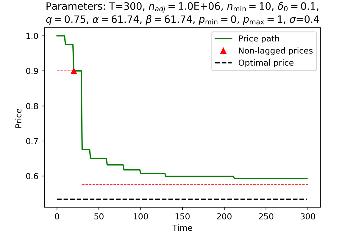
While Ada-LGD (Alg. 2) has optimal (up to logarithmic factors) regret as $T\to\infty$, its regret can be high for small values of $T$, since the number of samples taken at a point can be large relative to $T$ in this regime. To address this issue, we introduce an adjustment factor $n_{\text{adj}}$ and a minimum sampling rate $n_{\min}$. We re-define the sample size in Ada-LGD (Alg. 2) to be $n(d)=\max\Big{\{}\frac{64E_{\max}^{2}\log\frac{2}{p}}{Cn_{\text{adj}}\alpha^{2}d^{4}},n_{\min}\Big{\}}$.

We benchmark our algorithm against two bandit algorithms: a bandit convex optimization algorithm of [33] which is a sample-based gradient descent algorithm using a self-concordant barrier, and a UCB algorithm Discretize then UCB (Dtu) based on a discretization of $\mathcal{X}$. Dtu on input of $(\log T/T)^{1/3}$-discretization obtains a regret of $\widetilde{\mathcal{O}}(T^{2/3})$, which is sub-optimal, but nonetheless can have good performance. In our simulations, we use a discretization of 15 prices.

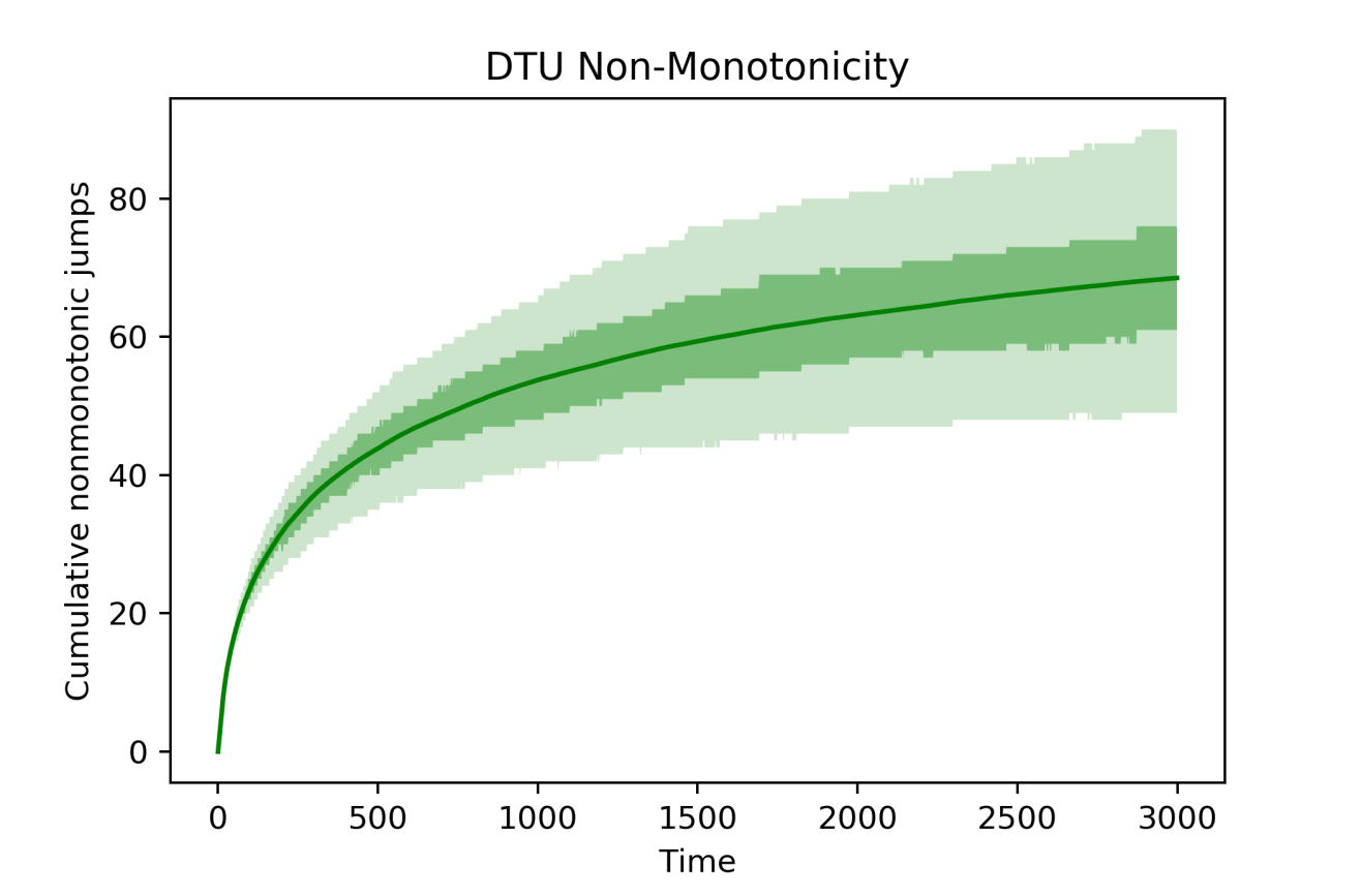
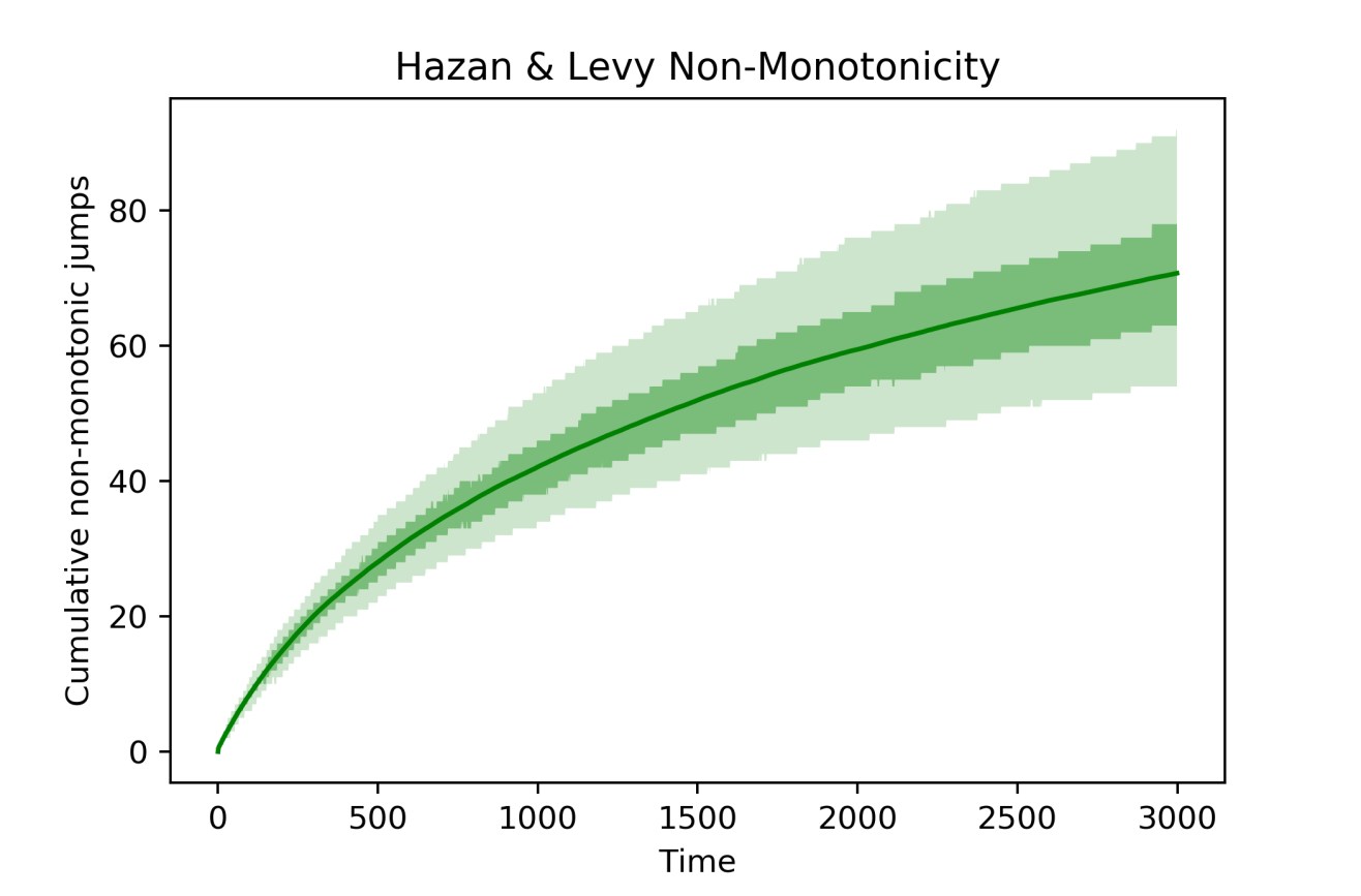
In Figure 6, we first plot the cumulative number of non-monotonic jumps for Hazan & Levy and Dtu. We note that both algorithms ultimately make a similar number of non-monotonic jumps at time 3000, with Dtu making most of these jumps in early time periods. A sample monotonic price path generated by Ada-LGD (Alg. 2) is shown in Figure 6 (right).

Figure 6: (left) The cumulative number of non-monotonic steps taken by Dtu. (center) The cumulative number of non-monotonic steps (green) and the cumulative number of non-monotonic steps of size at least $0.02$ (blue) generated by [33]. Both simulations were on input of data-derived revenue curves corrupted by independent $N(0,.4)$ noise over a price space of $[0,1]$. (right) Price path generated by Ada-Lgd (Alg. 2).

8 Discussion and Conclusion

There has been a surge of interest in the academic community and among policymakers alike on the topic of algorithmic fairness. As this discourse develops, various task-specific notions of fairness have been introduced. This is natural since the social backdrop of, say, loan-granting is very different from that of job applicant screening. Hence, the notions of fairness appropriate in various decision-making settings such as pricing, applicant screening, loan-granting, etc., may be different. However, these settings commonly involve decision-making over a period of time, and thus, the aspect of avoiding temporal disparity in decisions is common to most of these tasks. In this paper, we illustrated the rich interplay between temporal fairness desiderata and online decision-making through the novel meta-objective of ensuring fairness at the time of decision. There are several possibilities for extension of our proposal and analysis as we discuss below.

1. Envy freeness with multiplicative slacks. In many scenarios, multiplicative allowable disparities in treatment could be more appropriate than additive disparities. For example, a firm may want to price an item while ensuring that the price disparity between the youth and the general population is not more than 25%. In particular, consider slack functions $\bar{s}(\cdot,\cdot):\mathcal{I}\times\mathcal{I}\rightarrow\mathbb{R}^{\geq 0}$ defined on ordered pairs of groups, and consider the following definition of envy-freeness with multiplicative slacks.

   Definition 4 (Envy Freeness with Multiplicative Slacks)).

   We say that a decision vector $\mathbf{x}\in\mathcal{X}^{N}$ satisfies envy-freeness (EF) with multiplicative slacks if the following inequalities hold:

   $$x_{i}\geq\bar{s}(i,j)x_{j}\textrm{ for all }i,j\in\mathcal{I}.$$ (10)

   It would be interesting to extend our algorithm design to satisfy the FTD extension of this kind of a relaxed envy freeness constraint. One setting where our current results extend is the case where there is a function $m:\mathcal{I}\rightarrow\mathbb{R}^{>0}$ such that $\bar{s}(i,j)=m(j)/m(i)$. In this case, (10) effectively requires that $x_{i}m_{i}\geq x_{j}m_{j}$. In this case, one can redefine the decision space for group $i$ as $y_{i}=x_{i}m_{i}$. Our algorithms then readily apply to optimizing $\mathbf{y}$ in this setting.

2. Slack-monotonicity. In our analysis of envy freeness with additive slacks, we assumed that $s(i,i)=0$. This resulted in the temporal monotonicity constraint of ensuring $x_{i}(t)\geq x_{i}(t^{\prime})-s(i,i)=x_{i}(t^{\prime})$ for all $i$ and $t\geq t^{\prime}$. However, in many scenarios, some changes to within-group decisions across time may be acceptable. In other words, we may have $s(i,i)>0$ for all $i$, so that we effectively require that $x_{i}(t)$ is at most $s(i,i)$ lower than the highest decision seen by group $i$ until time $t$, thus allowing for a limited amount of backtracking in decisions (similarly, with multiplicative slacks, we may have that $s(i,i)<1$). While it is interesting that this type of slack in the monotonicity constraint isn’t necessary for our setting to attain the unconstrained optimal near-regret rate of $\widetilde{\mathcal{O}}(\sqrt{T})$, it may nevertheless simplify the algorithm design. Moreover, it may provide crucial flexibility in attaining near-optimal regret rates in harder settings, such as when the functions are only known to be unimodal.

3. Beyond strong convexity. It would be interesting to extend our results beyond the strong convexity assumption. As discussed earlier, for the simplest case of single-dimensional optimization, [36] and [37] have shown that a significant impact on the achievable rate of regret is inevitable under the monotonicity constraint if only unimodality and Lipschitzness of the cost function are assumed. While it seems that smoothness is necessary to obtain the near-optimal regret rate of $\widetilde{\mathcal{O}}(\sqrt{T})$ in our setting (since smoothness is fundamental to controlling overshooting of the optimum), we are hopeful that the strong convexity assumption can be relaxed (to, e.g., just assuming convexity) without impacting the regret guarantee.

4. Extensions to online convex optimization. It would be interesting to consider algorithm design for satisfying FTD in the general context of online convex optimization, which models scenarios where the utility function $\mathcal{U}$, though convex, changes over time [45]. In such scenarios, even with perfect gradient feedback (since the utility functions $U_{t}$ are assumed to be known in each period) it would be interesting to characterize conditions on the arriving functions under which sublinear regret rates can be attained while satisfying FTD.

5. Time decay. Certain fairness goals may not be subsumed by the FTD objective; as such, there is room for generalizing or adapting FTD to better fit specific objectives. For example, one may wish to incorporate a time-decay element to the envy-freeness constraint, which can be achieved by having the slack functions $s$ be dependent on the difference in the times at which the decisions were received by the two groups. In particular, we may have that $x_{i}(t)\geq x_{i}(t^{\prime})-s(i,i,t-t^{\prime})$ for all $t\geq t^{\prime}$, where the slack function now also takes the time difference $t-t^{\prime}$ as input. If $s$ is assumed to be increasing in the time difference, this would allow for greater changes in decisions over time.

Finally, we note that temporal considerations can be required or suggested for compliance with laws or policy. For example, applicant-screeners often ensure approximate demographic parity for the purpose of avoiding disparate impact litigation [46], and this constraint constrains current decisions by prior decisions. So-called “mandated progress” legislation, such as affirmative action—which has been adopted and, in some cases, mandated in the U.S., Canada, and France—can similarly be thought of as a temporal constraint in which goals must be set and a current decision is thus constrained by past decisions [47]. In terms of loan-granting, Wells Fargo was recently sued for racial dicrimination in mortgage lending, including offering different average interest rates to Black applicants than white applicants over a period of time [48], which again points to the potential for the use of temporal fairness constraints as a preventative measure for avoiding litigation. Some times these constraints can be enforced due to necessity of protecting consumer rights in the prevelant societal context, e.g., price gouging laws may dictate bounded increase in decisions, during the duration of the pandemic (McQueen and Ballinger v. Amazon.com). In general, the case law surrounding algorithmic approaches to ensuring fairness is not yet well-developed, thus leaving many questions open. However, we believe that it is important to get ahead of such restrictions and to understand the limitations of algorithms to provide guidance to legal scholarship on the possibilities.

Appendix A Missing analysis from Section 5

A.1 Useful lemmas.

We describe some useful results pertaining to any $\beta$-smooth and $\alpha$-strongly convex function $f$ that will be used in the analysis of our algorithms. The first is the fact that if $\nabla f(x)$ and $\nabla f(y)$ are close, then $x$ and $y$ are close as well, i.e., $\alpha|y-x|\leq|\nabla f(y)-\nabla f(x)|~{}\text{for all}~{}x,y\in\mathcal{P}$.

Lemma 2.

Let $f:\mathcal{K}\to\mathbf{R}$ be an $\alpha$-strongly convex function. Then

$$\|y-x\|\leq\frac{1}{\alpha}\|\nabla f(y)-\nabla f(x)\|~{},~{}~{}\text{ for all ~{}}~{}x,y\in\mathcal{K}.$$

Proof. Let $x,y\in\mathcal{K}$. If $x=y$, then the above inequality holds. So, we may assume that $x\neq y$. By strong convexity, we have

$$f(y)\geq f(x)+\nabla f(x)^{\top}(y-x)+\frac{\alpha}{2}\|y-x\|^{2},~{}\mbox{and}~{}f(x)\geq f(y)+\nabla f(y)^{\top}(x-y)+\frac{\alpha}{2}\|x-y\|^{2}.$$

Adding these two inequalities gives that

$$\|y-x\|^{2}\leq\frac{1}{\alpha}\langle\nabla f(x)-\nabla f(x),y-x\rangle\leq\frac{1}{\alpha}\|\nabla f(y)-\nabla f(x)\|\|y-x\|~{},$$

using Cauchy-Schwarz inequality. Finally, rearranging gives the desired result. ∎
Since $\beta$-smoothness is equivalent to $\beta$-Lipschitzness of the gradient (under the $L_{2}$ norm) we further have that $|\nabla f(y)-\nabla f(x)|\leq\beta|y-x|$ for all $x,y$.

Lemma 3 (general Hoeffding’s inequality [49]).

Let $\varepsilon_{1},\ldots,\varepsilon_{n}$ be independent mean-zero sub-Gaussian random variables. Then, there is a constant $C$ such that for every $s\geq 0$, we have

$$\mathbb{P}\Big{(}\Big{|}\sum_{t=1}^{n}\varepsilon_{i}\Big{|}\geq s\Big{)}\leq 2\exp\bigg{(}-\frac{Cs^{2}}{\sum_{t=1}^{n}\|\varepsilon_{i}\|_{\psi_{2}}^{2}}\bigg{)}.$$

Hoeffding’s inequality in turn helps us bound our errors in gradient estimation. In particular, the following key lemma shows that given enough samples at $x$ and $y$, one can obtain a secant estimate that is sandwiched between $\nabla f(x)$ and $\nabla f(y)$ with a high probability.

Lemma 4 (sandwich lemma).

Let $f:\mathbf{R}\to\mathbf{R}$ be an $\alpha$-strongly convex and $\beta$-smooth function, and let $x<y$. Suppose that querying $f$ at any point $z$ yields a noisy observation $f(z)+\varepsilon_{t}$ for the $t^{\textup{th}}$ sample, and suppose that the noise variables $\varepsilon_{1},\varepsilon_{2},\ldots$ satisfy Assumption 2. Now fix $p\in(0,1)$, and let $\overline{f}(x)$, $\overline{f}(y)$ be the averages of $\frac{64E_{\max}^{2}\log\frac{2}{p}}{C\alpha^{2}(y-x)^{4}}$ samples at $x$ and $y$, respectively, where $C$ is the absolute constant from Lemma 3. Then the estimated secant $g=\frac{\overline{f}(y)-\overline{f}(x)+\frac{\alpha(y-x)^{2}}{4}}{y-x}$ satisfies $\nabla f(x)\leq\frac{f(y)-f(x)}{y-x}\leq g\leq\nabla f(y)$, with probability at least $(1-p)^{2}$.

Proof. Let $\varepsilon=\alpha(y-x)^{2}/4$. Then by Hoeffding’s inequality (Lemma 3) with $n=\frac{64E_{\max}^{2}\log\frac{2}{p}}{C\alpha^{2}(y-x)^{4}}$,

$$\mathbb{P}\Big{(}|\overline{f}(x)-f(x)|\geq\varepsilon/2\Big{)}\leq 2\exp\Big{(}-\frac{C(\varepsilon/2)^{2}n}{E_{\max}^{2}}\Big{)}=p,$$

and similarly for $y$. So, we have that

$$\big{|}\overline{f}(x)-f(x)\big{|}\leq\frac{\varepsilon}{2}\quad\mbox{and}\quad\big{|}\overline{f}(y)-f(y)\big{|}\leq\frac{\varepsilon}{2}$$ (11)

with probability at least $(1-p)^{2}$. For the remainder of the proof, we assume that (11) holds.

We first bound $g-\frac{f(y)-f(x)}{y-x}$ from above and below:

$$g-\frac{f(y)-f(x)}{y-x} =\frac{\overline{f}(y)-\overline{f}(x)+\varepsilon}{y-x}-\frac{f(y)-f(x)}{y-x} g$$ (by definition of )

$$=\frac{1}{y-x}\Big{[}\big{(}\overline{f}(y)-f(y)\big{]}+\big{(}f(x)-\overline{f}(x)\big{)}+\varepsilon\Big{]}\in\left[0,\frac{2\varepsilon}{y-x}\right].$$

By definition of $\varepsilon$, this gives us:

$$0\leq g-\frac{f(y)-f(x)}{y-x}\leq\frac{\alpha}{2}(y-x)\qquad\mbox{with probability at least $(1-p)^{2}$.}$$ (12)

Since we have just shown that $g$ is close to the secant $\frac{f(y)-f(x)}{y-x}$, the only thing remaining is to show that $\nabla f(y)$ is sufficiently far away from the secant. We can do this by using strong convexity:

$$\frac{f(y)-f(x)}{y-x}\leq\frac{\nabla f(y)(y-x)-\frac{\alpha}{2}(y-x)^{2}}{y-x}=\nabla f(y)-\frac{\alpha}{2}(y-x).$$

We’ve thus shown that $0\leq g-\frac{f(y)-f(x)}{y-x}\leq\frac{\alpha}{2}(y-x)\leq\nabla f(y)-\frac{f(y)-f(x)}{y-x}.$ It follows that the estimated gradient $g$ satisfies $\nabla f(x)\leq\frac{f(y)-f(x)}{y-x}\leq g\leq\nabla f(y)$, where the first inequality follows from convexity, thus proving the lemma. ∎

A.2 Analysis for a single group

Proof of Lemma 1. We begin by proving “1.” To show that we never overshoot, we will exploit smoothness. In particular, for any $t$ such that $x_{t}\leq x^{*}$, we have

$$x_{t+1}-x_{t}^{\prime} =-\frac{1}{\beta}\widetilde{\nabla}_{t}=-\frac{1}{\beta}\nabla f(\overline{x_{t}}) \overline{x_{t}}\in[x_{t}^{\prime},x_{t}]$$ for some

$$=\frac{1}{\beta}\|\nabla f(\overline{x_{t}})\| x_{t}\leq x^{*}$$ since

$$\leq x^{*}-\overline{x_{t}} \nabla f(x^{*})=0$$ assuming

$$\leq x^{*}-x_{t}^{\prime}~{}.\text{This proves ``1.''}$$

To show the convergence (“2”), first note that by $\alpha$-strong convexity, we have that $f(y)\geq f(x)-\frac{1}{2\alpha}\|\nabla f(x)\|^{2}$. For $y=x^{*}$, this becomes:

$$\|\nabla f(x)\|^{2}\geq 2\alpha\big{[}f(x)-f(x^{*})\big{]}~{}.$$ (13)

Now we wish to bound the gap $h_{t}=f(x_{t})-f(x^{*})$. For any $t\geq 2$, we have

$$h_{t+1}-h_{t} =f(x_{t+1})-f(x_{t})$$

$$\leq\nabla_{t}^{\top}(x_{t+1}-x_{t})+\frac{\beta}{2}(x_{t+1}-x_{t})^{2} \beta$$ -smooth

$$\leq(\widetilde{\nabla}_{t}^{\top}+\beta\delta)(x_{t+1}-x_{t})+\frac{\beta}{2}(x_{t+1}-x_{t})^{2} \beta$$ -smooth

$$=-\frac{1}{2\beta}\|\widetilde{\nabla}_{t}\|^{2}-\delta\widetilde{\nabla}_{t}-\frac{\beta}{2}\delta^{2} x_{t+1}$$ definiton of

$$\leq-\frac{1}{2\beta}\|\widetilde{\nabla}_{t}\|^{2}-\left(-\frac{\widetilde{\nabla}_{t}}{(1+\gamma)\beta}\right)\widetilde{\nabla}_{t}-\frac{\beta}{2}\delta^{2} -\frac{1}{\beta}\widetilde{\nabla}_{t}\geq(1+\gamma)\delta$$ since

$$=-\left(\frac{1}{2\beta}-\frac{1}{(1+\gamma)\beta}\right)\|\widetilde{\nabla}_{t}\|^{2}-\frac{\beta}{2}\delta^{2}\leq-\underbrace{\left(\frac{1}{2\beta}-\frac{1}{(1+\gamma)\beta}\right)}_{=:c}\|\widetilde{\nabla}_{t}\|^{2}.$$

By the mean value theorem, there is some $\overline{x_{t}}\in[x_{t}^{\prime},x_{t}]\subset[x_{t-1},x_{t}]$ such that $\nabla f(\overline{x_{t}})=\widetilde{\nabla}_{t}$. Using 13, we get: $h_{t+1}-h_{t}\leq-c\|\widetilde{\nabla}_{t}\|^{2}=-c\|\nabla f(\overline{x_{t}})\|^{2}\overset{\ref{eqn:alpha-convex-rephrased-backtrack}}{\leq}-2\alpha c[f(\overline{x_{t}})-f(x^{*})]\leq-2\alpha ch_{t}.$ Note that for $\gamma>1$ as specified in the lemma, $2\alpha c\in(0,1)$. So,

$$h_{t+1} \leq\big{(}1-2\alpha c\big{)}h_{t}\leq\cdots\leq\big{(}1-2\alpha c\big{)}^{t}h_{1}\leq h_{1}\exp\big{(}-2\alpha ct\big{)}~{}.\qed$$

This convergence rate provides a regret bound for the noiseless single-group setting.

Proof of Theorem 1. As stated in the theorem, fix $\delta=T^{-1/2}$ as the lag size. Since overshooting never occurs (by Lemma 1), we need only calculate the exploration and stopping regret. By Lemma 1, the exploration regret is bounded by $2\sum_{t=1}^{\infty}h_{1}\exp\big{(}-2\alpha c(t-1)\big{)}$, which is constant.

Now we analyze the stopping regret. If the algorithm stops at some time $t$, then it must be that

$$-\frac{1}{\beta}\widetilde{\nabla}_{t}\leq(1+\gamma)\delta~{},$$

which allows us to bound the gradient: $\|\nabla_{t}\|\leq\|\widetilde{\nabla}_{t}\|\leq(1+\gamma)\delta$. In other words, if we stop at time $t$, then $\|\nabla_{t}\|\in\mathcal{O}(\delta)$, for $\gamma=1+\frac{1}{\log T}$. When $\|\nabla_{t}\|\leq 3\delta$, Lemma 2 tells us that $\|x_{t}-x^{*}\|\leq 3\delta/\alpha$, and so $f(x_{t})-f(x^{*})\in\mathcal{O}(\delta^{2})$ by $\beta$-smoothness. Hence,

$$\operatorname{regret}\leq\underbrace{2\sum_{t=1}^{\infty}h_{1}\exp\big{(}-2\alpha c(t-1)\big{)}}_{\in\mathcal{O}(1)}+\underbrace{T\delta^{2}}_{\in\mathcal{O}(1)}~{}.$$

So, we get a regret of $\mathcal{O}(1)$. ∎

Next, we analyze the single-group noisy algorithm (Algorithm 2). For the proof of Theorem 2, we introduce some additional notation for ease of exposition. Following our notion of phases, we can uniquely associate to each $x_{t}$ a pair $(s,i)$ such that $x_{t}$ is the $s$th iterate in the $i$th phase; we denote such an iterate as $x_{t}=y_{s}^{(i)}$. So, e.g., in Figure 2, we see that $x_{1}=y_{1}^{(1)},x_{2}=y_{1}^{(2)},x_{3}=y_{2}^{(2)},x_{4}=y_{1}^{(3)}$ and $x_{5}=y_{1}^{(4)}$. We now proceed with the proof.

We break the proof into several claims. We refer to the estimated gradient at the $\delta_{i}$-lagged point: $g_{t}^{(i)}=\frac{\overline{f}(x_{t}-\delta_{i+1})-\overline{f}(x_{t}-\delta_{i})+\varepsilon(\xi\delta_{i})}{\xi\delta_{i}}$; and the probability parameter of the algorithm: $p=T^{-2}$.

Claim 3 (gradient accuracy).

Let $\widetilde{\widetilde{\nabla}}_{t}=\frac{\overline{f}(x_{t})-\overline{f}(x_{t}-\delta_{i})+\varepsilon(\delta_{i})}{\delta_{i}}$ be the estimated secant at epoch $t$, and let $g_{t}^{(i)}=\frac{\overline{f}(x_{t}-\delta_{i+1})-\overline{f}(x_{t}-\delta_{i})+\varepsilon(\xi\delta_{i})}{\xi\delta_{i}}$, where $\delta_{i}=q^{i-1}\delta_{1}$ is the $i^{\text{th}}$ lag size and $\xi=1-q$. Then these gradient estimates of the algorithm satisfy

$$\widetilde{\widetilde{\nabla}}_{t}\in[\nabla f(x_{t}-\delta_{i}),\nabla f(x_{t})]\quad\mbox{and}\quad g_{t}^{(i)}\in[\nabla f(x_{t}-\delta_{i}),\nabla f(x_{t}-\delta_{i+1})].$$ (14)

each with probability at least $(1-p)^{2}$, where $p=T^{-2}$.

Note that for this choice of $p$, we have that $(1-p)^{T}\to 1$. This claim follows immediately from Lemma 4 since each of the estimates is constructed by sampling $\frac{4E_{\max}^{2}\log\frac{2}{p}}{C\varepsilon(d)^{2}}$ times, where $\varepsilon(d)=\alpha d^{2}/4$ and $d$ is the gap between the two points at which we are sampling (i.e., $d=\delta_{i}$ in the case of $\widetilde{\widetilde{\nabla}}_{t}$ and $d=\xi\delta_{i}$ in the case of $g_{t}^{(i)}$).

Claim 4 (overshooting).

Assuming (14) holds for all estimated gradients, and that $x_{1}=x_{\min}+\delta_{1}<x^{*}$, then all the iterates $x_{1},x_{2},\ldots x_{k}$ (for $k\leq T$) generated by the lagged secant movements in the outer loop of the algorithm do not overshoot the optimum; that is, $x_{t}\leq x^{*}$ for all $t\leq k$. Note that this implies that all lagged points sampled by the algorithm (i.e., those sampled between $x_{t}$ and $x_{t+1}$, for some $t$) also do not overshoot.

Proof of Claim 4. We show this by induction, where the base case follows from assumption that $x_{1}\leq x^{*}$. Suppose $x_{t}\leq x^{*}$, and that $x_{t+1}$ was chosen based on a lag size of $\delta_{i}$. In other words, $x_{t+1}=x_{t}-\frac{1}{\beta}\widetilde{\widetilde{\nabla}}_{t}-\delta_{i}$, where $\widetilde{\widetilde{\nabla}}_{t}=\frac{\overline{f}(x_{t})-\overline{f}(x_{t}-\delta_{i})+\varepsilon(\delta_{i})}{\delta_{i}}$ and $\varepsilon(\delta_{i})=\alpha\delta_{i}^{2}/4$. By (14) and the mean value theorem, $\widetilde{\widetilde{\nabla}}_{t}=\nabla f(\overline{x}_{t})$ for some $\overline{x}_{t}\in[x_{t}-\delta_{i},x_{t}]$. So,

$$x_{t+1}-(x_{t}-\delta_{i}) =-\frac{1}{\beta}\widetilde{\widetilde{\nabla}}_{t}=-\frac{1}{\beta}\nabla f(\overline{x}_{t}) \overline{x}_{t}\in[x_{t}-\delta_{i},x_{t}]$$ for some

$$=\frac{1}{\beta}|\nabla f(\overline{x}_{t})| x_{t}\leq x^{*}$$ since

$$\leq x^{*}-\overline{x}_{t} \nabla f(x^{*})=0 f$$ since and is smooth

$$\leq x^{*}-(x_{t}-\delta_{i}).$$

This proves Claim 4. $\hfill\qed_{\text{Claim \ref{claim:overshooting}}}$

Claim 5 (monotonicity).

Assuming (14) holds for all estimated gradients, and that $x_{1}<x^{*}$, samples taken by the algorithm (including lagged and non-lagged iterates) are non-decreasing.

Proof of Claim 5. Again, suppose that $x_{t+1}$ was chosen based on a lag size of $\delta_{i}$. In other words, $x_{t+1}=x_{t}-\frac{1}{\beta}\widetilde{\widetilde{\nabla}}_{t}-\delta_{i}$, where $\widetilde{\widetilde{\nabla}}_{t}\leftarrow\frac{\overline{f}(x_{t})-\overline{f}(x_{t}-\delta_{i})+\varepsilon(\delta_{i})}{\delta_{i}}$ and $g_{t}^{(i)}=\frac{\overline{f}(x_{t}-\delta_{i+1})-\overline{f}(x_{t}-\delta_{i})+\varepsilon\big{(}\xi\delta_{i}\big{)}}{\xi\delta_{i}}$, where $\delta_{i}=q^{i-1}\delta_{1}$ is the $i$th lag sizes and $\xi=1-q$. Note that $\xi\delta_{i}=(x_{t}-\delta_{i+1})-(x_{t}-\delta_{i})$ is the domain gap between $x_{t}-\delta_{i}$ and $x_{t}-\delta_{i+1}$. To show monotonicity, we need to show that the next lagged point exceeds the current point; i.e., we must show that $x_{t}\leq x_{t+1}-\delta_{i}$.

Note that the lagged step is taken only for the first $\delta_{i}$ that achieves $-\frac{1}{\beta}g_{t}^{(i)}\geq(2+\gamma)\delta_{i}$. So,

$$-\frac{1}{\beta}\widetilde{\widetilde{\nabla}}_{t} \geq-\frac{1}{\beta}\nabla f(x_{t})$$ by grad. bounds (14)

$$\geq-\frac{1}{\beta}\left(\nabla f(x_{t}-\delta_{i})+\beta\delta_{i}\right) \beta$$ -smoothness

$$\geq-\frac{1}{\beta}\left(g_{t}^{(i)}+\beta\delta_{i}\right)$$ by grad. bounds (14)

$$\geq(1+\gamma)\delta_{i}$$ by assumption.

Since $\gamma>1$ by assumption, we have that $(x_{t+1}-\delta_{i})-x_{t}=-\frac{1}{\beta}\widetilde{\widetilde{\nabla}}_{t}-2\delta_{i}\geq(1+\gamma)\delta_{i}-2\delta_{i}>0$. In other words, we do not break monotonicity. This proves Claim 5. $\hfill\qed_{\text{Claim \ref{claim:monotonicity}}}$

Claim 6 (convergence rate).

Assume (14) holds for all estimated gradients, and that $x_{1}<x^{*}$. Now let $h_{t}=f(x_{t})-f(x^{*})$ be the instantaneous regret at $x_{t}$. Then $h_{t+1}\leq h_{1}\exp(-2\alpha ct)$, where $c=\frac{1}{2\beta}-\frac{1}{(1+\gamma)\beta}$. In particular, letting $h_{t}^{(i)}=f(y_{t}^{(i)})-f(x^{*})$ be the instantaneous regret at the $t$th point of the $i$th phase, we have that

$$h^{(i)}_{t+1}\leq h^{(i)}_{1}\exp\big{(}-2\alpha ct\big{)}\quad\mbox{(Phase $i$ convergence),}$$ (15)

when at least $t+1$ distinct, non-lagged points are sampled in Phase $i$. Moreover, across non-trivial phases, we get a cumulative contraction:

$$h^{(i)}_{1}\leq h^{(1)}_{1}\exp\big{(}-2\alpha ck_{i}\big{)}\quad\mbox{when $k_{i}$ distinct non-lagged points are sampled up to Phase $i$.}$$ (16)

Consequently, since each phase contains at least one non-lagged point,

$$h^{(i)}_{1}\leq h^{(1)}_{1}\exp\big{(}-2\alpha c(i-1)\big{)}\quad\mbox{(inter-phase convergence).}$$ (17)

Proof of Claim 6. To show the exponential convergence rate in Claim 6, we will show that the improvement $h_{t}-h_{t+1}$ at time $t$ is of order at least (approximately) $|\nabla f(x_{t})|^{2}$. This will imply, by the strong convexity assumption, a contraction in $h_{t}$, which gives us an exponential rate of convergence. To that end, suppose we jump from $x_{t}$ using a lag size of $\delta_{i}$; in other words, suppose $x_{t+1}=x_{t}-\frac{1}{\beta}\widetilde{\widetilde{\nabla}}_{t}-\delta_{i}$. Then the following holds:

$$h_{t+1}-h_{t} =f(x_{t+1})-f(x_{t})$$ (18)

$$\leq\nabla_{t}^{\top}(x_{t+1}-x_{t})+\frac{\beta}{2}(x_{t+1}-x_{t})^{2} \beta$$ -smooth (19)

$$\leq(\widetilde{\widetilde{\nabla}}_{t}^{\top}+\beta\delta_{i})(x_{t+1}-x_{t})+\frac{\beta}{2}(x_{t+1}-x_{t})^{2}$$ by (14) (20)

$$=(\widetilde{\widetilde{\nabla}}_{t}^{\top}+\beta\delta_{i})(-\widetilde{\widetilde{\nabla}}_{t}-\delta_{i})+\frac{\beta}{2}(-\widetilde{\widetilde{\nabla}}_{t}-\delta_{i})^{2}$$ (21)

$$=-\frac{1}{2\beta}\|\widetilde{\widetilde{\nabla}}_{t}\|^{2}-\delta_{i}\widetilde{\widetilde{\nabla}}_{t}-\frac{\beta}{2}\delta_{i}^{2}\leq-\frac{1}{2\beta}\|\widetilde{\widetilde{\nabla}}_{t}\|^{2}-\left(-\frac{\widetilde{\widetilde{\nabla}}_{t}}{(1+\gamma)\beta}\right)\widetilde{\widetilde{\nabla}}_{t}-\frac{\beta}{2}\delta_{i}^{2}$$ (22)

$$=-\left(\frac{1}{2\beta}-\frac{1}{(1+\gamma)\beta}\right)\|\widetilde{\widetilde{\nabla}}_{t}\|^{2}-\frac{\beta}{2}\delta_{i}^{2}\leq-\underbrace{\left(\frac{1}{2\beta}-\frac{1}{(1+\gamma)\beta}\right)}_{=:c}\|\widetilde{\widetilde{\nabla}}_{t}\|^{2}.$$ (23)

By (14) and the mean value theorem, there is some $\overline{x}_{t}\in[x_{t}-\delta_{i},x_{t}]\subset[x_{t-1},x_{t}]$ such that $\nabla f(\overline{x}_{t})=\widetilde{\widetilde{\nabla}}_{t}$, which gives:

$$h_{t+1}-h_{t}\leq-c\|\widetilde{\widetilde{\nabla}}_{t}\|^{2}=-c\|\nabla f(\overline{x}_{t})\|^{2}\overset{\ref{eqn:alpha-convex-rephrased-backtrack}}{\leq}-2\alpha c[f(\overline{x}_{t})-f(x^{*})]\leq-2\alpha ch_{t},\mbox{~{}since we do not overshoot.}$$

Since $\gamma>1$ (as specified in the algorithm), $2\alpha c=\frac{2\alpha}{2\beta}-\frac{2\alpha}{(1+\gamma)\beta}\leq\frac{\alpha}{\beta}\in(0,1)$ (since $\alpha\leq\beta$). So,

$$h_{t+1} \leq\big{(}1-2\alpha c\big{)}h_{t}\leq\cdots\leq\big{(}1-2\alpha c\big{)}^{t}h_{1}\leq h_{1}\exp\big{(}-2\alpha ct\big{)}~{}.$$

The contractions in (15)-(16) follow immediately, and (17) follows from the fact that if $y_{1}^{(i)}=x_{t}$ and $y_{1}^{(i+1)}=x_{s}$, then $t<s$. $\hfill\qed_{\text{Claim \ref{claim:convergence}}}$

Claim 7 (regret from gradient descent jumps).

Assume (14) holds for all estimated gradients, and that $x_{1}<x^{*}$. Then, let $\operatorname{regret}_{\textsc{Lgd}}(k)$ be the total regret incurred during the first $k$ phases on the points $x_{t}$, as well as the two lagged points just after $x_{t}$ (see the boxed points in Figure 2); i.e., $\operatorname{regret}_{\textsc{Lgd}}(k)$ is the regret incurred during the following samplings:

• the $\frac{64E_{\max}^{2}\log\frac{2}{p}}{C\alpha^{2}\delta_{n_{i}}^{4}}$ samples at $x_{s}=y_{t}^{(i)}$,

• the $\frac{64E_{\max}^{2}\log\frac{2}{p}}{C\alpha^{2}\xi^{4}\delta_{n_{i}}^{4}}$ samples at $x_{s+1}-\delta_{n_{i}}$, and

• the first $\frac{64E_{\max}^{2}\log\frac{2}{p}}{C\alpha^{2}\xi^{4}\delta_{n_{i}}^{4}}$ samples at $x_{s+1}-\delta_{n_{i}+1}$,

for phases $i\in[k]$ (for any $k$) and their respective $t^{\text{th}}$ points. Then $\operatorname{regret}_{\textsc{Lgd}}(k)$ during the first $k$ phases is of order $\mathcal{O}\left(\frac{h\log\frac{1}{p}}{\delta_{1}^{4}}+\log\frac{1}{p}\sum_{i=1}^{k}\frac{1}{|\nabla f(y_{1}^{(i+1)})|^{2}}\right)$.

Proof of Claim 7. As we progess toward the optimum, we potentially use smaller and smaller lag sizes. This results in cumbersome sampling when close to the optimum. To prove Claim 7, we will use the exponential decay of instantaneous regret to allay some of this regret. Additionally, we will show that the instantaneous regret during Phase $i$ is of order $\delta_{n_{i}}^{2}$; since the gradient at $y_{1}^{(i)}$ is of order $\delta_{n_{i}}$, this fact will ultimately ultimately allow us to bound $\operatorname{regret}_{\textsc{Lgd}}$ in terms of gradients.

Recall that we are bounding regret incurred during the first $k$ phases only, as stated in the claim. Let $q$ be the contraction in the lag sizes, i.e., $\delta_{i+1}=q\delta_{i}$. We will bound the regret at $x_{t},x_{t+1}-\delta_{i},x_{t+1}-\delta_{i+1}$; among these three points, the instantaneous regret is highest at $x_{t}$, so we simply bound the instantaneous regret at each of these points by $h_{t}$. For any $i$, let $T^{(i)}$ be the index of the last point in Phase $i$; i.e., $y_{T^{(i)}}^{(i)}$ is the last point in Phase $i$. The number of samples at each of these three points is bounded by $\frac{64E_{\max}^{2}\log\frac{2}{p}}{C\alpha^{2}\xi^{4}\delta_{n_{i}}^{4}}$, so this in turn gives us the following upper bound, where $h=f(x_{\min})-f(x^{*})$:

$$\operatorname{regret}_{\textsc{Lgd}} \leq\frac{128E_{\max}^{2}\log\frac{2}{p}}{C\alpha^{2}\xi^{4}\delta_{1}^{4}}h+\sum_{i=1}^{k}\frac{192E_{\max}^{2}\log\frac{2}{p}}{C\alpha^{2}\xi^{4}\delta_{n_{i}}^{4}}\sum_{t=1}^{T^{(i)}}h_{t}^{(i)}$$ (24)

$$=\frac{128E_{\max}^{2}\log\frac{2}{p}}{C\alpha^{2}\xi^{4}\delta_{1}^{4}}h+\sum_{i=1}^{k}\frac{192E_{\max}^{2}\log\frac{2}{p}}{C\alpha^{2}\xi^{4}q^{4n_{i}}\delta_{1}^{4}}\sum_{t=1}^{T^{(i)}}h_{t}^{(i)}$$ (25)

$$=\frac{128E_{\max}^{2}\log\frac{2}{p}}{C\alpha^{2}\xi^{4}\delta_{1}^{4}}h+\frac{192E_{\max}^{2}\log\frac{2}{p}}{C\alpha^{2}\xi^{4}\delta_{1}^{4}}\sum_{i=1}^{k}\frac{1}{q^{4n_{i}}}\sum_{t=1}^{T^{(i)}}h_{t}^{(i)}$$ (26)

$$\leq\frac{128E_{\max}^{2}\log\frac{2}{p}}{C\alpha^{2}\xi^{4}\delta_{1}^{4}}h+\frac{192E_{\max}^{2}\log\frac{2}{p}}{C\alpha^{2}\xi^{4}\delta_{1}^{4}}\sum_{i=1}^{k}\frac{1}{q^{4n_{i}}}\sum_{t=1}^{T^{(i)}}h^{(i)}_{1}\exp\big{(}-2\alpha c(t-1)\big{)}$$ by (15) (27)

$$=\frac{128E_{\max}^{2}\log\frac{2}{p}}{C\alpha^{2}\xi^{4}\delta_{1}^{4}}h+\frac{192E_{\max}^{2}\log\frac{2}{p}}{C\alpha^{2}\xi^{4}\delta_{1}^{4}}\sum_{i=1}^{k}\frac{1}{q^{4n_{i}}}h^{(i)}_{1}\sum_{t=1}^{T^{(i)}}\exp\big{(}-2\alpha c(t-1)\big{)}$$ (28)

$$\leq\frac{128E_{\max}^{2}\log\frac{2}{p}}{C\alpha^{2}\xi^{4}\delta_{1}^{4}}h+\frac{192E_{\max}^{2}\log\frac{2}{p}}{C\alpha^{2}\xi^{4}\delta_{1}^{4}\big{(}1-e^{-2\alpha c}\big{)}}\sum_{i=1}^{k}\frac{1}{q^{4n_{i}}}h^{(i)}_{1}.$$ (29)

To continue this analysis, we bound $h_{1}^{(i)}$. To that end note that $|\nabla f(y_{1}^{(i)})|<\beta(2+\gamma)\delta_{n_{i}-1}$, since a previous secant $g$ must have satisfied $-\frac{1}{\beta}g<(2+\gamma)\delta_{n_{i}-1}$. So, assuming the gradient $g$

$$\beta(2+\gamma)\delta_{n_{i}-1}\overset{(a)}{>}|\nabla f(y_{1}^{(i)})|=|\nabla f(y_{1}^{(i)})-\nabla f(x^{*})|\overset{(b)}{\geq}{\alpha}|x^{*}-y_{1}^{(i)}|,$$ (30)

where $(a)$ follows from the fact that $|\nabla f(y_{1}^{(i)})|<|\nabla f(y_{1}^{(i)}-\delta_{j})|\leq|g|$ for some $j$ (by (14)), and $(b)$ follows from strong-convexity. Finally, by smoothness, we have

$$h_{1}^{(i)}\overset{(c)}{\leq}\frac{\beta}{2}(x^{*}-y_{1}^{(n_{i})})^{2}\overset{\eqref{eqn:bounding-gap-by-distance}}{<}\frac{\beta^{3}(2+\gamma)^{2}}{2\alpha^{2}}\delta_{n_{i}-1}^{2}=\frac{\beta^{3}(2+\gamma)^{2}}{2q^{2}\alpha^{2}}\delta_{n_{i}}^{2},$$ (31)

again where $(c)$ follows from smoothness (assuming $\nabla f(x^{*})=0$).

Continuing the analysis from above, we have

$$\operatorname{regret}_{\textsc{Lgd}} \leq\frac{128E_{\max}^{2}\log\frac{2}{p}}{C\alpha^{2}\xi^{4}\delta_{1}^{4}}h+\frac{192E_{\max}^{2}\log\frac{2}{p}}{C\alpha^{2}\xi^{4}\delta_{1}^{4}\big{(}1-e^{-2\alpha c}\big{)}}\sum_{i=1}^{k}\frac{1}{q^{4n_{i}}}h^{(i)}_{1}$$ (32)

$$\leq\frac{128E_{\max}^{2}\log\frac{2}{p}}{C\alpha^{2}\xi^{4}\delta_{1}^{4}}h+\frac{96E_{\max}^{2}\beta^{3}(2+\gamma)^{2}\log\frac{2}{p}}{C\alpha^{4}\xi^{4}\delta_{1}^{4}\big{(}1-e^{-2\alpha c}\big{)}q^{2}}\sum_{i=1}^{k}\frac{\delta_{n_{i}}^{2}}{q^{4n_{i}}}$$ (33)

$$=\frac{128E_{\max}^{2}\log\frac{2}{p}}{C\alpha^{2}\xi^{4}\delta_{1}^{4}}h+\frac{96E_{\max}^{2}\beta^{3}(2+\gamma)^{2}\log\frac{2}{p}}{C\alpha^{4}\xi^{4}\delta_{1}^{2}\big{(}1-e^{-2\alpha c}\big{)}q^{2}}\sum_{i=1}^{k}\frac{q^{2n_{i}}}{q^{4n_{i}}}$$ (34)

$$=\frac{128E_{\max}^{2}\log\frac{2}{p}}{C\alpha^{2}\xi^{4}\delta_{1}^{4}}h+\frac{96E_{\max}^{2}\beta^{3}(2+\gamma)^{2}\log\frac{2}{p}}{C\alpha^{4}\xi^{4}\delta_{1}^{2}\big{(}1-e^{-2\alpha c}\big{)}q^{2}}\sum_{i=1}^{k}\frac{1}{q^{2n_{i}}}.$$ (35)

At this point, for convenience, we will replace $\frac{1}{q^{2n_{i}}}$ with a gradient estimate. In particular, let $x_{t_{i}}=y_{1}^{(i+1)}$ be the iterate at which we jump using $\delta_{n_{i+1}}$ for the first time. Then it must be that $|\nabla f(x_{t_{i}})|<\beta(2+\gamma)\delta_{n_{i}}$, or in other words, $q^{n_{i}}>\frac{|\nabla f(x_{t_{i}})|}{\beta(2+\gamma)\delta_{1}}$. So, continuing the inequalities above,

$$\operatorname{regret}_{\textsc{Lgd}} \leq\frac{128E_{\max}^{2}\log\frac{2}{p}}{C\alpha^{2}\xi^{4}\delta_{1}^{4}}h+\frac{96E_{\max}^{2}\beta^{3}(2+\gamma)^{2}\log\frac{2}{p}}{C\alpha^{4}\xi^{4}\delta_{1}^{2}\big{(}1-e^{-2\alpha c}\big{)}q^{2}}\sum_{i=1}^{k}\frac{1}{q^{2n_{i}}}$$ (36)

$$\leq\frac{128E_{\max}^{2}\log\frac{2}{p}}{C\alpha^{2}\xi^{4}\delta_{1}^{4}}h+\frac{96E_{\max}^{2}\beta^{5}(2+\gamma)^{4}\log\frac{2}{p}}{C\alpha^{4}\xi^{4}\big{(}1-e^{-2\alpha c}\big{)}q^{2}}\sum_{i=1}^{k}\frac{1}{|\nabla f(x_{t_{i}})|^{2}}.$$ (37)

$\hfill\qed_{\text{Claim \ref{claim:regret-lgd}}}$

Figure 7: Points sampled while transitioning from lag size $\delta_{n_{i}}$.

Claim 8 (regret from transitioning lag sizes).

Assume (14) holds for all estimated gradients, and that $x_{1}<x^{*}$. Here we bound the regret which is unaccounted for in Claim 7; i.e., we bound the regret incurred at exploratory lagged points. More precisely, let $\operatorname{regret}_{\delta\text{-transition}}(k)$ be the regret incurred from sampling at $y_{1}^{(i+1)}-\delta_{n_{i}+1},\ldots,y_{1}^{(i+1)}-\delta_{n_{i+1}+1}$ for $1\leq i\leq k$. Then, $\operatorname{regret}_{\delta\text{-transition}}(k)\in\mathcal{O}\left(\log\frac{1}{p}\sum_{i=1}^{k}\frac{1}{|\nabla f(y_{1}^{(i+1)})|^{2}}\right)$, for any $k\leq T$.

Proof of Claim 8. Here we bound the regret incurred while transitioning lag sizes (e.g., the regret from the samples taken at points which do not appear in boxes in Figure 2). In order to bound the regret resulting from $\delta$-transitions, we argue that whenever we transition from phase $n_{i}$, the current gradient is small in magnitude compared to $\delta_{n_{i}}$. This allows us to bound the number of lagged points sampled during any transitions from $\delta_{n_{i}}$ to $\delta_{n_{i+1}}$, which in turn gives us a bound on the total regret resulting from these transitions.

Let $t_{1},\ldots,t_{k}$ be such that $x_{t_{i}}=y_{1}^{(i+1)}$. To bound the regret from transitioning lag sizes, let us consider the regret incurred transitioning from $\delta_{n_{i}}$ to $\delta_{n_{i+1}}$, which happens at time $t_{i}$ (note that $n_{i}$ and $n_{i+1}$ are not consecutive if the algorithm goes down multiple lag sizes during the same round). The regret incurred from transitioning to $\delta_{n_{i+1}}$ is the regret incurred at $x_{t_{i}}-\delta_{n_{i}+1},x_{t_{i}}-\delta_{n_{i}+2},\ldots x_{t_{i}}-\delta_{n_{i+1}+1}$ (see Figure 7). Let us begin by bounding the number of lag sizes that can be passed in one round. Suppose we sample at $x_{t_{i}}-\delta_{n_{i}+j}$ and decide to decrease the lag size to $\delta_{n_{i}+j}$. In other words, we observe that

$$-\frac{1}{\beta}\cdot\underbrace{\frac{\overline{f}(x_{t_{i}}-\delta_{n_{i}+j})-\overline{f}(x_{t_{i}}-\delta_{n_{i}+j-1})+\varepsilon(\xi\delta_{n_{i}+j-1})}{\xi\delta_{n_{i}+j-1}}}_{=:g}<(2+\gamma)\delta_{n_{i}+j-1}$$ (38)

and therefore need to begin sampling at $x_{t_{i}}-\delta_{n_{i}+j+1}$. In this case, observe that

$$|\nabla f(x_{t_{i}})|\overset{(a)}{\leq}|g|\overset{(b)}{\leq}\beta(2+\gamma)\delta_{n_{i}+j-1}=\beta(2+\gamma)q^{j-1}\delta_{n_{i}}.$$

where $(a)$ follows from (14) and $(b)$ from (38). Thus for $J_{i}=\max\left\{2,~{}\left\lceil\frac{1}{\log q}\log\left(\frac{|\nabla f(x_{t_{i}})|}{\beta(2+\gamma)\delta_{n_{i}}}\right)\right\rceil+1\right\}$, we will not transition; i.e., $n_{i+1}<n_{i}+J_{i}$ and we will not sample at $x_{t_{i}}-\delta_{n_{i}+J_{i}+1}$.

Next, we will bound the instantaneous regret incurred by sampling at $x_{t_{i}}-\delta_{n_{i}+j}$. Suppose we have just transitioned to $\delta_{n_{i}+j}$, and must now sample at $x_{t_{i}}-\delta_{n_{i}+j}$ and $x_{t_{i}}-\delta_{n_{i}+j+1}$ in order to determine whether or not to reduce the lag size further. Since we have just transitioned to $\delta_{n_{i}+j}$, we know that (38) holds. This in turn implies that

$$|\nabla f(x_{t_{i}}-\delta_{n_{i}+j})|\leq|g|<\beta(2+\gamma)q^{j-1}\delta_{n_{i}}.$$

So, the regret we get from each sample (whether at $x_{t_{i}}-\delta_{n_{i}+j}$ or $x_{t_{i}}-\delta_{n_{i}+j+1}$), is bounded by

$$f(x_{t_{i}}-\delta_{n_{i}+j})-f(x^{*})\leq\frac{\beta}{2\alpha}\Big{[}\beta(2+\gamma)q^{j-1}\delta_{n_{i}}\Big{]}^{2}=\frac{\beta^{3}(2+\gamma)^{2}q^{2(j-1)}\delta_{n_{i}}^{2}}{2\alpha}.$$ (39)

We can now calculate our regret from lag transitions as follows:

$$\operatorname{regret}_{\delta\mbox{-transition}} \leq\sum_{i=1}^{k}\sum_{j=1}^{J_{i}}\frac{128E_{\max}^{2}\log\frac{2}{p}}{C\alpha^{2}\xi^{4}\delta_{n_{i}+j}^{4}}\cdot\Big{[}f(x_{t_{i}}-\delta_{n_{i}+j})-f(x^{*})\Big{]}$$ (40)

$$\leq\sum_{i=1}^{k}\sum_{j=1}^{J_{i}}\frac{128E_{\max}^{2}\log\frac{2}{p}}{C\alpha^{2}\xi^{4}\delta_{n_{i}+j}^{4}}\cdot\frac{\beta^{3}(2+\gamma)^{2}q^{2(j-1)}\delta_{n_{i}}^{2}}{2\alpha}$$ by (39) (41)

$$=\frac{64E_{\max}^{2}\beta^{3}(2+\gamma)^{2}\log\frac{2}{p}}{C\alpha^{3}\xi^{4}q^{2}}\sum_{i=1}^{k}\frac{1}{\delta_{n_{i}}^{2}}\sum_{j=1}^{J_{i}}\frac{1}{q^{2j}}$$ (42)

$$\leq\frac{64E_{\max}^{2}\beta^{3}(2+\gamma)^{2}\log\frac{2}{p}}{C\alpha^{3}\xi^{4}q^{2}\left(\frac{1}{q^{2}}-1\right)}\sum_{i=1}^{k}\frac{1}{\delta_{n_{i}}^{2}}\frac{1}{q^{2(J_{i}+1)}}$$ (43)

$$=\frac{64E_{\max}^{2}\beta^{3}(2+\gamma)^{2}\log\frac{2}{p}}{C\alpha^{3}\xi^{4}q^{8}\left(\frac{1}{q^{2}}-1\right)}\sum_{i=1}^{k}\frac{1}{\delta_{n_{i}}^{2}}\frac{1}{q^{2(J_{i}-2)}}$$ (44)

$$=\frac{64E_{\max}^{2}\beta^{3}(2+\gamma)^{2}\log\frac{2}{p}}{C\alpha^{3}\xi^{4}q^{8}\left(\frac{1}{q^{2}}-1\right)}\sum_{i=1}^{k}\frac{1}{\delta_{n_{i}}^{2}}e^{(\log q^{-2})(J_{i}-2)}$$ (45)

$$=\frac{64E_{\max}^{2}\beta^{3}(2+\gamma)^{2}\log\frac{2}{p}}{C\alpha^{3}\xi^{4}q^{8}\left(\frac{1}{q^{2}}-1\right)}\sum_{i=1}^{k}\frac{1}{\delta_{n_{i}}^{2}}e^{(\log q^{-2})\left(\left\lceil\frac{1}{\log q}\log\left(\frac{|\nabla f(x_{t_{i}})|}{\beta(2+\gamma)\delta_{n_{i}}}\right)\right\rceil-1\right)}$$ (46)

$$\leq\frac{64E_{\max}^{2}\beta^{3}(2+\gamma)^{2}\log\frac{2}{p}}{C\alpha^{3}\xi^{4}q^{8}\left(\frac{1}{q^{2}}-1\right)}\sum_{i=1}^{k}\frac{1}{\delta_{n_{i}}^{2}}e^{(\log q^{-2})\left(\frac{1}{\log q}\log\left(\frac{|\nabla f(x_{t_{i}})|}{\beta(2+\gamma)\delta_{n_{i}}}\right)\right)}$$ (47)

$$\leq\frac{64E_{\max}^{2}\beta^{3}(2+\gamma)^{2}\log\frac{2}{p}}{C\alpha^{3}\xi^{4}q^{8}\left(\frac{1}{q^{2}}-1\right)}\sum_{i=1}^{k}\frac{1}{\delta_{n_{i}}^{2}}e^{2\log\left(\frac{\beta(2+\gamma)\delta_{n_{i}}}{|\nabla f(x_{t_{i}})|}\right)}$$ (48)

$$=\frac{64E_{\max}^{2}\beta^{3}(2+\gamma)^{2}\log\frac{2}{p}}{C\alpha^{3}\xi^{4}q^{8}\left(\frac{1}{q^{2}}-1\right)}\sum_{i=1}^{k}\frac{1}{\delta_{n_{i}}^{2}}\left(\frac{\beta(2+\gamma)\delta_{n_{i}}}{|\nabla f(x_{t_{i}})|}\right)^{2}$$ (49)

$$=\frac{64E_{\max}^{2}\beta^{5}(2+\gamma)^{4}\log\frac{2}{p}}{C\alpha^{3}\xi^{4}q^{8}\left(\frac{1}{q^{2}}-1\right)}\sum_{i=1}^{k}\frac{1}{|\nabla f(x_{t_{i}})|^{2}}.$$ (50)

$\hfill\qed_{\text{Claim \ref{claim:regret-delta-transition}}}$

Claim 9 (total regret).

Assume (14) holds for all estimated gradients, and that $x_{1}<x^{*}$. Then the regret is of order $(\log T)^{2}T^{1/2}$, for $\delta_{1}=1/\log T$, $p=T^{-\lambda}$ for $\lambda>3/2$, and $\gamma=1+\frac{1}{\log T}$.

Proof of Claim 9. The expressions of regret in Claims 7 and 8 grow rapidly as $k$ increases, so we only use these expressions to bound regret in early phases. For later phases, we argue that the gradient is small, which gives us a bound on the late-phase regret. Balancing the regret between early and late stages ultimately achieves the claimed $\widetilde{\mathcal{O}}(T^{1/2})$ regret bound.

In particular, we will break the regret from the $\delta$-transition into two categories: the regret when the gradient is small ($|\nabla f(x_{t_{i}})|\leq T^{-d}$) and the regret when the gradient is large ($|\nabla f(x_{t_{i}})|>T^{-d}$). If $k_{d}$ is the number of $\delta$-transitions until $|\nabla f(x_{t_{i}})|\leq T^{-d}$, then $k_{d}$ is of order $\log T$. To show this precisely, observe that

$$|\nabla f(x_{t_{i}})|^{2} \leq\frac{2\beta^{2}}{\alpha}\big{(}f(x_{t_{i}})-f(x^{*})\big{)} +$$ smth str. convexity

$$\leq\frac{2\beta^{2}h_{1}^{(1)}}{\alpha}e^{-2\alpha c(i-1)}.$$

So, if $i>\frac{1}{\alpha c}\left(\frac{1}{2}\log\frac{2\beta^{2}h_{1}^{(1)}}{\alpha}+d\log T\right)+1$, then $|\nabla f(x_{t_{i}})|\leq T^{-d}$. In turn, if $|\nabla f(x_{t_{i}})|\leq T^{-d}$, then

$$f(x_{t_{i}})-f(x^{*}) \leq\frac{\beta}{2\alpha^{2}}T^{-2d},$$

by smoothness and strong convexity. Now, define $\operatorname{regret}_{\delta\mbox{-transition}}$ to be the total regret from transitioning lag sizes over all iterations; that is, if $m$ is the last phase of the algorithm (which is well-defined since number of iterations is bounded by $T$), then $\operatorname{regret}_{\delta\mbox{-transition}}=\operatorname{regret}_{\delta\mbox{-transition}}(m)$. Then we can bound $\operatorname{regret}_{\delta\mbox{-transition}}$ as

$$\operatorname{regret}_{\delta\mbox{-transition}} =\operatorname{regret}_{\delta\mbox{-transition}}(k_{d})+\Big{[}\operatorname{regret}_{\delta\mbox{-transition}}-\operatorname{regret}_{\delta\mbox{-transition}}(k_{d})\Big{]}$$

$$\leq\frac{64E_{\max}^{2}\beta^{5}(2+\gamma)^{4}\log\frac{2}{p}}{C\alpha^{3}\xi^{4}q^{8}\left(\frac{1}{q^{2}}-1\right)}k_{d}T^{2d}+\frac{\beta}{2\alpha^{2}}T^{1-2d}.$$

Setting $d=1/4$ and bounding $k_{d}$ by $\left\lceil\frac{1}{\alpha c}\left(\frac{1}{2}\log\frac{2\beta^{2}h_{1}^{(1)}}{\alpha}+d\log T\right)\right\rceil+2$, we get that

$$\operatorname{regret}_{\delta\mbox{-transition}}\in\mathcal{O}\Big{(}(\log T)^{2}T^{1/2}\Big{)}.$$

Since $\operatorname{regret}_{\textsc{Lgd}}$ is of the same order as $\operatorname{regret}_{\delta\mbox{-transition}}$ (ignoring the lower-order term $\frac{h\log\frac{1}{p}}{\delta_{1}^{4}}$),

$$\operatorname{regret} \leq(1-p)^{T}\Big{[}\operatorname{regret}_{\textsc{Lgd}}+\operatorname{regret}_{\delta\mbox{-transition}}\Big{]}+\Big{(}1-(1-p)^{T}\Big{)}T$$

$$\in\mathcal{O}\left((1-p)^{T}(\log T)^{2}T^{1/2}+\Big{(}1-(1-p)^{T}\Big{)}T\right)$$

$$=\mathcal{O}\left(\big{(}1-o(1)\big{)}(\log T)^{2}T^{1/2}+o(T^{1/2})\right),$$

for $p=T^{-\lambda}$, $\lambda>3/2$. This gives us a regret bound of $\mathcal{O}\left((\log T)^{2}T^{1/2}\right)$. ∎

A.3 Analysis for two groups

Algorithm 3 is composed of two phases: (1) a coordinate descent phase, in which Ada-LGD (Alg. 2) is run separately on the two groups, and the group being optimized changes each time a lag size is contracted; and (2) a combined phase, where the decisions for one group are locked with respect to the decisions for the other, and the two are optimized simultaneously. For simplicity, we will assume that at each queried point $(x_{1},x_{2})$, feedback is observed and regret is incurred for both groups. Without this assumption, the regret will increase by a $\widetilde{\mathcal{O}}(1)$ factor dependent on $\min_{i\in\{1,2\}}a_{i}$, where $a$ is the distribution over groups. Much of the analysis is identical to that of Algorithm 2; as such, we focus on the differences, and break up the argument into claims.

Figure 8: Decision space $\mathcal{X}_{F}^{N}$ with the following scenario in Alg. 3: Group 2 has undergone at least one lag size transition and Group 1 is at a tight constraint. X’s represent lagged points, filled-in circles the non-lagged points, and empty circles the feasibility iterates; gradients of $f_{1}$ are estimated at red nodes, and gradients of $f_{2}$ are estimated at blue nodes. $g_{1},\ldots,g_{4}$ denote gradient estimates obtained from the two nodes indicated by the brackets. The orange square of side length $D\big{(}\delta^{(2)}\big{)}$ is relevant to Claims 10-11.

Claim 10.

Suppose $\delta^{(2)}<\delta$ is the lag size for Group 2, and Group 1 has hit the boundary of the feasible region (see Fig. 8) at $(x^{(1)},x^{(2)})$. Then the following hold with probability at least $(1-p)^{4}$:

• if $x^{*}_{1}-x_{1}\leq D(\delta^{(2)})$, then the algorithm does not enter the combined phase; and

• if $x^{*}_{1}-x_{1}\geq D(\delta^{(2)})+H(\delta^{(2)})$, then the algorithm enters the combined phase.

Proof of Claim 10. First suppose that $x^{*}_{1}-x_{1}\leq D(\delta^{(2)})$. Then by smoothness, we have that $|f_{1}^{\prime}(x_{1})|\leq\beta D(\delta^{(2)})=(2+\gamma)\frac{\beta^{2}}{\alpha}\cdot\frac{\delta^{(2)}}{q}$. Now let $g_{1}$ be the gradient estimate obtained from points $x_{1}-\delta^{(2)}$ and $x_{1}-q\delta^{(2)}$, as shown in Figure 8. Then

$$-\frac{1}{\beta}g_{1} =\frac{1}{\beta}|g_{1}|\leq\frac{1}{\beta}|f_{1}^{\prime}(x_{1}-\delta^{(2)})|\leq\frac{1}{\beta}|f_{1}^{\prime}(x_{1})|+\delta\leq D(\delta^{(2)})+\delta^{(2)}=(2+\gamma)\frac{\beta}{\alpha}\cdot\frac{\delta^{(2)}}{q}+\delta^{(2)}$$

with probability at least $(1-p)^{2}$. In this case, the algorithm does not enter the combined phase.

Now suppose that $x^{*}_{1}-x_{1}\geq D(\delta^{(2)})+H(\delta^{(2)})$. Expanding this expression, we get that $x^{*}_{1}-x_{1}\geq(2+\gamma)\frac{\beta^{2}}{\alpha^{2}}\cdot\frac{\delta^{(2)}}{q}+\frac{\beta\delta^{(2)}}{\alpha}$. This implies by strong convexity that

$$|f_{1}^{\prime}(x)|\geq(2+\gamma)\frac{\beta^{2}}{\alpha}\cdot\frac{\delta^{(2)}}{q}+\beta\delta^{(2)}.$$

Since $|g_{1}|>|f_{1}^{\prime}(x)|$ with probability at least $(1-p)^{2}$, it follows that $-\frac{1}{\beta}g_{1}\geq(2+\gamma)\frac{\beta}{\alpha}\cdot\frac{\delta^{(2)}}{q}+\delta^{(2)}$ with the same probability. Hence, in this case, the algorithm will enter the combined phase. $\hfill\qed_{\text{Claim \ref{claim:transitioning-to-combined}}}$

Claim 11.

Let $g_{1}$ be the gradient estimated at the feasibility iterates (see Figure 8), and let $z^{*}=(x_{1}^{*},x_{2}^{*})$ be the unconstrained optimum.

• If $z^{*}\in\mathcal{X}_{F}^{2}$, then the algorithm never enters the combined phase.

• If the algorithm enters the combined phase based on the gradient estimate $g_{1}$ (as in Fig. 8), then $-\frac{1}{\beta}g_{1}\geq(2+\gamma)\delta^{(2)}$.

Proof of Claim 11. We begin with the first claim. It is enough to show that Group 1 sampling will not induce a transition to the combined phase, given that Group 2 has already undergone at least one lag size transition. As in Claim 11, let $\delta^{(2)}<\delta$ be the current lag size of Group 2. We will argue that the Group 2 gradient must be small, since this group has transitioned from the previous lag size $\delta^{(2)}/q$; thus, the optimum $x_{2}^{*}$ of $f_{2}$ must be close to the current point $x_{2}$.

To that end, let $g_{4}$ be the gradient which induced the transition to $\delta^{(2)}$ (see, e.g., Fig. 8). It follows that $-\frac{1}{\beta}g_{4}<(2+\gamma)\frac{\delta^{(2)}}{q}$. Let $y$ be the non-lagged iterate corresponding to $g_{4}$ (so, in Fig. 8, $y=x_{2}$). Then $\alpha|x^{*}_{2}-y|\leq|f_{2}^{\prime}(y)|<|g_{4}|<(2+\gamma)\beta\delta^{(2)}/q$. It follows that

$$|x^{*}_{2}-x_{2}|\leq|x^{*}_{2}-y|<(2+\gamma)\frac{\beta}{\alpha}\cdot\frac{\delta^{(2)}}{q}=D\big{(}\delta^{(2)}\big{)}.$$ (51)

Since we are assuming that $z^{*}\in\mathcal{X}_{F}^{2}$, it must be that $|x^{*}_{1}-x_{1}|\leq D\big{(}\delta^{(2)}\big{)}$ as well. Thus, by Claim 10, the algorithm will not enter the combined phase with high probability.

To prove the second statement, let $g_{1}$ be the gradient estimate (in the Group 1 direction) which induced the transition to the combined phase (see, e.g., Fig. 8). Then, since $\alpha\leq\beta$ and $0<q<1$,

$$-\frac{1}{\beta}g_{1}\geq\left(\frac{(2+\gamma)\beta}{q\alpha}+1\right)\delta^{(2)}>(2+\gamma)\delta.$$

In other terms, since the algorithm transitions to the combined phase only when the gradient in the Group 1 direction is large enough, a lag size transition will not be triggered. $\hfill\qed_{\text{Claim \ref{claim:combined-phase-monotonicity}}}$

Claim 12.

The feasibility check iterates (e.g., the brown nodes in Figure 3) increase the overall regret during the coordinate phase by at most a factor of two.

Proof of Claim 12. Feasibility check iterates are sampled $\widetilde{\mathcal{O}}(1/\delta_{i}^{4})$ times, where $\delta_{i}$ is the current lag size of the other group. Thus the regret incurred at the two feasibility check iterates is strictly less than the regret incurred at the previous two lagged iterates in the other group. $\hfill\qed_{\text{Claim \ref{claim:checking-feasibility check-is-fast}}}$

Claim 13.

Let $\delta_{n_{1}}>\cdots>\delta_{n_{m}}$ be the distinct non-trivial lag sizes of Group $j$ (excluding $\delta$ if $\delta$ is a non-trivial lag size), where $\delta_{i}=q^{i}\delta$. Defining $n_{0}=0$, we have that $n_{i+1}-n_{i}\in\mathcal{O}(1)$ for $0\leq i<m$. Moreover, the number of gradient-scaled jumps taken with lag size $\delta_{n_{i}}$ is constant as well, for $1\leq i\leq m$.

Proof of Claim 13. Let us begin by bounding $n_{i+1}-n_{i}$, for $i\geq 1$. Let $x_{t_{i+1}}$ denote the first non-lagged iterate which admits a lag size of $\delta_{n_{i+1}}$. In this case, the previous non-lagged iterate $x$ admitted a lag size of $\delta_{n_{i}}$. We can show that the gradient estimate $g$ at $x$ is an underestimate (in magnitude) by $\mathcal{O}(\delta_{n_{i}})$:

$$g\geq\frac{f_{j}(x)-f_{j}(x-\delta_{n_{i}})}{\delta_{n_{i}}}\geq\nabla f_{j}(x-\delta_{n_{i}})+\frac{\alpha}{2}\delta_{n_{i}}$$

by the Sandwich Lemma (Lem. 4) and strong convexity. Thus $x_{t_{i+1}}$ must be shy of the optimum by at least $\Omega(\delta_{n_{i}})$, and thus has gradient of order $\Omega(\delta_{n_{i}})$. Since the gradient changes by at most a constant factor from $x$ to $x_{t_{i+1}}$, the number $n_{i+1}-n_{i}$ of transient lag sizes must also be constant.

The above argument can be extended to bound $n_{1}$ as well. If the initial lag size of $\delta$ was non-trivial (i.e., some gradient-scaled jump was made using a lag size of $\delta$), then the above argument hold verbatim. Otherwise, the initial non-lagged iterate $({x_{\min}}+\delta)$ has a gradient of magnitude $\mathcal{O}(\delta)$. However, since $\delta=1/\log T$ and the optimum is assumed to be strictly greater than zero, we may assume that $T$ is large enough so that the gradient at ${x_{\min}}+\delta$ is large with respect to $\delta$.

Finally, we argue the “moreover” claim. While $\delta_{n_{i}}$ is the lag size, the gradient has magnitude $\Theta(\delta_{n_{i}})$. Once the gradient drops below $\mathcal{O}(q\delta_{n_{i}})$, a lag transition is initiated. Since the gradient-scaled jumps yield linear convergence, $t$ jumps with lag size $\delta_{n_{i}}$ would yield instantaneous regret of order $e^{-t}\delta_{n_{i}}^{2}$. For $t\in\mathcal{O}(1)$, this would result in an instantaneous regret of order $(q\delta_{n_{i}})^{2}$, which would trigger a lag size transition. $\hfill\qed_{\text{Claim \ref{claim:regularity-of-transitions}}}$

Claim 14.

The waiting regret (i.e., the regret incurred by Group 1 over the blue nodes and by Group 2 over the red nodes in Figure 3) is $\widetilde{\mathcal{O}}(T^{1/2})$.

Proof of Claim 14. Note that smaller lag sizes require more sampling: if $\delta^{(2)}<\delta^{(1)}$, then more time will be spend sampling $f_{2}$ at $x_{2}-\delta^{(2)}$ and $x_{2}-q\delta^{(2)}$ than will be spent sampling $f_{1}$ at $x_{1}-\delta^{(1)}$ and $x_{1}-q\delta^{(1)}$. In order to capture worst-case waiting regret for a group, we will consider the case where $\delta^{(2)}\leq\delta^{(1)}$ at all times and bound the waiting regret of Group 1.

Let $\delta_{n_{1}}>\cdots>\delta_{n_{m}}$ be the non-trivial lag sizes used by Group 2 (excluding $\delta$, if $\delta$ is a non-trivial lag size). Note that $\delta_{n_{1}}$ is not necessarily $\delta$, and $\delta_{n_{i+1}}/\delta_{n_{i}}$ is not necessarily $q$. For each $i$, let $T_{i}$ denote the number of samples taken where $\delta_{n_{i}}$ is the lag size or in transitioning to $\delta_{n_{i+1}}$. Thus, letting $T_{0}$ denote the number of samples prior to $\delta_{n_{1}}$, we have that $\sum_{i=0}^{m}T_{i}=T$.

We will now bound the waiting regret of Group 1 during these $m+1$ phases. First, consider the time period associated with $T_{i}$, for any $1\leq i\leq m$. During this phase, Group 2 has already transition to a lag size of $\delta_{n_{i}}$ from a lag size of $\delta_{n_{i}}/q$. Note that once this transition is made, the algorithm switches to optimizing over Group 1. Since the algorithm did not enter the combined phase in the previous round, it must be that the gradient in the Group 1 direction is of order $\delta_{n_{i}}$. Thus, the total waiting regret for Group 1 is of order

$$T_{0}+\sum_{i=1}^{m}T_{i}\delta_{n_{i}}^{2}~{}.$$

Now let us consider bounds on $T_{i}$, for $0\leq i\leq m$. By Claim 13, we know that the number of gradient-scaled jumps that Group 2 takes during this phase is constant, and similarly the number of lags transitions (i.e., $n_{i+1}-n_{i}$) is also constant. It follows that $T_{i}\in\widetilde{\mathcal{O}}(\delta_{n_{i}}^{-4})$.

We can similarly bound $T_{0}$. As in the previous calculations, we will ignore constants for simplicity. To bound $T_{0}$, we first bound the number of gradient-scaled jumps before the current gradient is of order $q\delta$ (as this would trigger a lag size transition). To that end, the linear convergence rate of Ada-LGD (Alg. 2) implies that the gradient after $t$ gradient-scaled jumps is of order $e^{-t}M^{2}$, where $M=\max_{(x,y)\in{\mathcal{X}_{F}^{2}}}|f_{2}^{\prime}(y)|$. It follows that the gradient is of order $q\delta$ after $\ln\frac{M}{q\delta}$ jumps; since $\delta=1/\log T$, the total number of gradient-scaled jumps before the first lag size transition is of order $\log\log T$. Finally, by Claim 13, $n_{1}$ is constant as well, which implies that $T_{0}\in\mathcal{O}\big{(}(\log T)^{5}\log\log T\big{)}$.

Putting all of this together, the waiting regret for Group 1 is of soft order $\sum_{i=1}^{m}\delta_{n_{i}}^{-2}$. Letting $x_{2,t_{i}}$ denote the first non-lagged iterates for Group 2 to admit a lag size of $\delta_{n_{i}}$, we have that $|\nabla f_{2}(x_{2,t_{i}})|\in\Theta(\delta_{n_{i}})$. Thus we can rewrite the waiting regret for Group 1 as $\sum_{i=1}^{m}1/|\nabla f_{2}(x_{2,t_{i}})|^{2}$. Finally, since we stop optimizing over Group 2 when its gradient is bounded in magnitude by $T^{-1/4}$, we can bound this further by $mT^{1/2}$. Since there can be at most logarithmically many gradient-scaled jumps before the gradient is of order $T^{-1/4}$, the waiting regret is $\widetilde{\mathcal{O}}(T^{1/2})$. $\hfill\qed_{\text{Claim \ref{claim:waiting-regret}}}$

Since the combined function $h$ is $\alpha$-strongly convex and $\beta$-smooth, we have the same convergence rate for the combined phase as before. Moreover, since the algorithm does not erroneously enter the combined phase with high probability, the optimum of $h$ is the same as the constrained optimum with high probability. Thus, the regret analysis of Algorithm 2 carries over. ∎

Appendix B Algorithm and analysis from Section 6

We first introduce some notation that will be used in the multi-group algorithm (Algorithm 4). The first is the succession function, which cycles between the different clusters of groups.

Definition 5 (succession function).

Let $N\in\mathbb{N}$ and let $\Pi$ be a partition of $[N]$. For any $A\in\Pi$, define the successor $\varphi(A;\Pi):=\begin{cases}\operatorname*{arg\,min}_{B\in\Pi:\min B>\min A}\min B&\mbox{if $\exists B\in\Pi$ with $\min B>\min A$}\\ \operatorname*{arg\,min}_{B\in\Pi}\min B&\mbox{else.}\end{cases}$

Note that $\varphi(\,\cdot\,;\Pi)$ corresponds to the linear ordering of $\Pi$ by the minimum elements of its blocks.

Next, we define the feasibility distance, which quantifies the extent to which a cluster $A$ can move without violating any of the constraints.

Definition 6 (feasibility distance).

Let $N\in\mathbb{N}$, let $\emptyset\neq A\subsetneq[N]$, let $s:[N]\times[N]\to\mathbb{R}^{\geq 0}$, and let $x\in\mathbb{R}^{N}$ satisfy. Then the feasibility distance of $A$ is $d(A;x)=\min_{i\in A,j\not\in A}x_{j}+s(i,j)-x_{i}$.

With these definitions in mind, we outline our $N$-group algorithm, Cycle-then-Combine Lagged Gradient Descent (C²-Lgd) (Alg. 4). The high-level idea of the algorithm is to maintain a clustering (i.e., a partition) of the groups, optimize each cluster separately in coordinate-descent fashion, and combine clusters whenever none can move and doing so would loosen a tight constraint. These ideas are described in more detail below.

Making gradient-scaled jumps. As with all other algorithms presented in this paper, gradients are estimated using a lagged and non-lagged point. However, while Ada-Lgd and SCAda-Lgd used adaptive lag size, C²-Lgd uses a fixed lag size $\delta$, which greatly simplifies algorithm design and analysis. In C²-Lgd, whenever a cluster’s gradient becomes smaller than $\mathcal{O}(\delta)$, it can no longer move without risking breaking monotonicity, so it is no longer optimized in isolation (although it may be optimized further after being combined with another cluster).

Switching between clusters. Since all clusters have the same lag size, each cluster takes the same number of samples to make a gradient-scaled jump. Thus, there is no concern over one cluster obtaining copious amounts of regret while another cluster is sampling at a single point. We can therefore employ a simple trigger: switch to the next cluster after (1) a point has been sampled, or (2) the boundary has been hit.

Combining clusters. Suppose we have reached a point where no cluster can move. If all clusters are at a low gradient, then we have reached an approximate optimum, and no further movements are made. Otherwise, there are clusters at tight constraints. In this can, we argue that there must be a low-gradient cluster which is preventing a tight cluster from moving without violated the EF constraint. In this case, we combine two such clusters and continue.

input : Number of groups $N$, sub-Gaussian norm bound $E_{\max}$, $n(d)=\frac{64E_{\max}^{2}\log\frac{2}{p}}{C\alpha^{2}d^{4}}$, smoothness parameter $\beta$ and strong convexity parameter $\alpha$ of $f(x_{1},\ldots,x_{N})=\sum_{i=1}^{N}f_{i}(x_{i})$, time horizon $T$, non-negative FTP slacks $s$, $x_{\min}$, $\gamma$, lag size $\delta$

1 Initialize queue $Q_{i}\leftarrow\emptyset$ for $i\in[N]$ // will contain points to query

2 Initialize the partition $\Pi=\big{\{}\{1\},\ldots,\{N\}\big{\}}$ of groups, and set $\textup{active}_{A}=\textup{Yes}$ and $g_{A}=-\infty$ for each $A\in\Pi$

3 For any $A\subseteq[N]$, define $f_{A}(x)=\sum_{i\in A}f_{i}(x)$; initialize $A=\{1\}$

4 Add $x_{\min}$, $x_{\min}+\delta$ to $Q_{i}$ for $i\in[N]$

5 while fewer than $T$ samples have been taken do

6        if $\textup{active}_{B}=\textup{No}$ for each cluster $B\in\Pi$ (i.e., no clusters can move) then

7               if each cluster is constrained by some other cluster then

8                      Find clusters $C,D$ which are locked in place with respect to each other (see Claim 15)

9               else

10                      Find clusters $C\neq D\in\Pi$ such that $C$ is at a tight constraint imposed by some group in $D$, and $D$ has met the small gradient condition (see Claim 15)

11              Update $\Pi\leftarrow\Pi\cup\{C\cup D\}\setminus\{C,D\}$

12               Let $A=C\cup D$, and set $g_{A}=-\infty$ and $\textup{active}_{A}=\textup{Yes}$

13               Let $i=\min A$, and add $x_{i},x_{i}+\delta$ to $Q_{i}$ // add points to the representative group’s queue

14       Let $i=\min A$ // choose a representative group

15        $\mathcal{X}_{A}=[x_{i},x_{i}+d(A;x)]$ // current feasible points for cluster $A$

16        if $Q_{i}$ contains any elements in $\mathcal{X}_{A}$ then

17               Let $x_{i}\leftarrow\min Q_{i}$, remove $x_{i}$ from $Q_{i}$, and update $x_{j}$ (for $j\in A\setminus\{i\}$) accordingly (i.e., letting $d=\min Q_{i}-x_{i}$, we set $x_{j}\leftarrow x_{j}+d$ for all $j\in A$)

18               Update $\textup{active}_{B}$ for $B\in\Pi$ as necessary (formerly tight clusters may now be active; in particular, if $B$ is at a tight constraint imposed by some group in $A$ and $B$ is not at any tight constraints imposed by any group in any other cluster, then $B$ will no longer be at a tight constraint)

19              Sample $n(\delta)$ times at $x_{j}$ for $j\in A$

20               if $x_{i}$ is a non-lagged iterate for cluster $A$ then

21                      Update the gradients $g^{(i)}$ for $i\in A$ and set $g_{A}=\sum_{i\in A}g^{(i)}$

22                      if $-\frac{1}{\beta}g_{A}\geq(1+\gamma)\delta$ then

23                             Add $x_{i}-2\delta-\frac{1}{\beta}g_{A}$ and $x_{i}-\delta-\frac{1}{\beta}g_{A}$ to $Q_{i}$

24                            

25                      else

26                             Set $\textup{active}_{A}=\textup{No}$

27                     

28              

29       if $Q_{i}$ contains no elements in $\mathcal{X}_{A}$ then

30               Set $x_{i}=\max\mathcal{X}_{A}$ and update $x_{j}$ (for $j\in A$) accordingly

31               Set $\textup{active}_{A}=\textup{No}$ and update $\textup{active}_{B}$ for $B\in\Pi$ (formerly tight clusters may now be active)

32       

33       if $-\frac{1}{\beta}g_{B}<(1+\gamma)\delta$ for every cluster $B\in\Pi$ then

34               Exit the while loop and remain at point $x$ for the remaining iterations

35       $A\leftarrow\varphi(A;\Pi)$ // move to the next group

36       

37

Algorithm 4 Cycle-then-Combine Lagged Gradient Descent (C²-Lgd)

Proof of Theorem 4 First, we argue that Algorithm 4 run on a single group would result in $\widetilde{\mathcal{O}}(T^{2/3})$ regret. To that end, we bound the pre-stopping regret and the post-stopping regret separately. Since the convergence rate is exponential, the number of queried points is bounded by a constant. Since each point is queried $\widetilde{\mathcal{O}}(\delta^{-4})$ times, the total regret from exploration is $\widetilde{\mathcal{O}}(\delta^{-4})$. Next, since the algorithm stops when the gradient is of order $\delta$, the instantaneous stopping regret is of order $\delta^{2}$. Since overshooting is avoided with high probability, the total regret is $\widetilde{\mathcal{O}}(\delta^{-4}+T\delta^{2})=\widetilde{\mathcal{O}}(T^{2/3})$. Next, we return to the $N$-group setting. Before bounding the regret, we prove that the algorithm never encounters a situation where all clusters are constrained by each other.

Claim 15.

Suppose the condition at line 6 (that no clusters can move and not all clusters are at a low gradient) is satisfied. Then either (1) some subset of clusters is locked in place with respect to each other (i.e., their joint feasible decisions form a line), or (2) some cluster must be at a low-gradient condition and constraining the movement of another cluster.

To prove this claim, suppose (1) does not hold, and suppose $C_{1},\ldots,C_{k}$ are the current clusters. For each $j\in[k]$, let $i_{j}=\min C_{j}$ be a representative group from cluster $C_{j}$. We can therefore represent the constraints placed on $C_{j}$ by linear inequalities on $x_{i_{j}}$; i.e., for each $j\neq m\in[k]$, there exist $b_{j,m}\in\mathbb{R}$ such that

$$x_{i_{j}}\leq x_{i_{m}}+b_{j,m}$$

is the constraint placed on $C_{i_{j}}$ by $C_{i_{m}}$. Moreover, since the slacks $s(\cdot,\cdot)$ are nonnegative, $b_{j,m}\geq 0$.

Now consider the directed graph $G=(\{C_{1},\ldots,C_{k}\},A)$, where the arc $(C_{i_{j}},C_{i_{m}})$ means that $C_{i_{j}}$ is constrained by $C_{i_{m}}$ (i.e., $x_{i_{j}}=x_{i_{m}}+b_{j,m}$). We now argue that this graph must be acyclic. For the sake of contradiction, suppose that there is a cycle $(j_{1},\ldots,j_{\ell})$; i.e.,

$$x_{i_{j_{1}}} =x_{i_{j_{2}}}+b_{j_{1},j_{2}}$$

$$\vdots$$

$$x_{i_{j_{\ell-1}}} =x_{i_{j_{\ell}}}+b_{j_{\ell-1},j_{\ell}}$$

$$x_{i_{j_{\ell}}} =x_{i_{j_{1}}}+b_{j_{\ell},j_{1}}.$$

This implies that $x_{i_{j_{1}}}\geq\cdots\geq x_{i_{j_{\ell}}}\geq x_{i_{j_{1}}}$. If these inequalities are all equalities, this contradicts our assumption that (1) does not hold; otherwise, if one of the inequalities is strict, this also yields a contradiction. Thus, $G$ is acyclic.

Now, choose any cluster $C$ which has at least one out-going arc (which must exist, since not all clusters are at a low gradient). Find a maximal directed path beginning at $C$, and let $(C_{i_{j}},C_{i_{m}})$ be the terminal arc. Since $G$ is acyclic, there are no out-going arcs from $C_{i_{m}}$, which means that $C_{i_{m}}$ is at a low gradient and is constraining the movement of $C_{i+j}$. This proves the claim.

The previous claim shows that the algorithm operates without getting stuck. Next, we bound the cluster-combining regret and stopping regret separately.

Regret from erroneously combining clusters.

Claim 2. The total regret incurred due to erroneously combining clusters (i.e., combining clusters whose joint unconstrained optimum is in the interior of the feasible region) is of order $\widetilde{\mathcal{O}}(N^{3}T\delta^{2})$.

To justify Claim 2, first note that clusters are combined at most $N-1$ times throughout a run of the algorithm. We define $f^{1}_{i}=f_{i}$ to be the initial group-specific functions. Each time clusters are combined, we define a new set of functions which are “close” to the previous set of functions, and for which the clusters were combined correctly.

Suppose that clusters have been combined $k$ times, and the current partition of the groups is $\mathcal{C}_{k}=\{C^{k}_{1},\ldots,C^{k}_{N-k}\}$. For any cluster $C$, we define $\min C$ to the the representative group of that cluster. Thus, there exists a sequence of gaps $\eta\in\mathbb{R}^{N}$ such that the function evaluation at a point $x\in\mathbb{R}$ for cluster $C$ can be expressed as

$$f^{k}_{C}(x,\eta^{k}):=\sum_{j\in C}f^{k}_{j}(x+\eta^{k}_{j}).$$

Suppose we are combining clusters $C$ and $D$ at the representative points $(x_{t},y_{t})$. Without loss of generality, suppose $C$ is tight and $D$ is at a low gradient. Then the slacks $s$ and the current lockings induce linear constraints $x\leq y+b_{C,D}$ and $y\leq x+b_{D,C}$ for some $b_{C,D},b_{D,C}\geq 0$, where $x$ is the representative decision for cluster $C$, and $y$ for cluster $D$. Since $C$ is tight, we have that $x_{t}=y_{t}+b_{C,D}$, and since $D$ is at a low gradient condition, $|(f^{k}_{D})^{\prime}(y_{t},\eta^{k})|\in\mathcal{O}(\delta)$ with high probability.

Let $\mathcal{X}_{C,D}$ be the polyhedron in $\mathbb{R}^{2}$ defined by the constraint imposed on $C$ by $D$ and vice versa (i.e., the gray region in Figure 5). Now let $(x^{\prime},y^{\prime})=\operatorname*{arg\,min}_{(x,y)}f^{k}_{C}(x,\eta^{k})+f^{k}_{D}(y,\eta^{k})$. With high probability, we have not overshot in either the $C$ or the $D$ direction. So, if $(x^{\prime},y^{\prime})\not\in\mathcal{X}_{C,D}$, then we have correctly combined the clusters. Otherwise, $(x^{\prime},y^{\prime})\in\mathcal{X}_{C,D}$ (see Figure 5 for a depiction of this scenario). In this case, $|y^{\prime}-y_{t}|\in\mathcal{O}(\delta)$ and $|x^{\prime}-x_{t}|\in\mathcal{O}(\delta)$. So, letting $(w_{1},w_{2})$ be the projection of $(x^{\prime},y^{\prime})$ onto the facet $x=y+b_{C,D}$, and letting $(\rho,\rho)=(x^{\prime},y^{\prime})-(w_{1},w_{2})$, we have that $\rho\in\mathcal{O}(\delta)$.

Now let $\eta^{k+1}$ be the new gaps after combining clusters $C$ and $D$. To account for the $\mathcal{O}(\delta)$ error from combining $C$ and $D$, we consider a new function

$$f^{k+1}_{C\cup D}(x,\eta^{k+1})=\sum_{i\in C\cup D}f_{i}^{k+1}(x+\eta_{j}),$$

where $f_{i}^{k+1}(x)=f_{i}^{k}(x+\rho)$. For all other clusters $E$, we define $f^{k+1}_{E}=f^{k}_{E}$. Thus, with high probability, according to the functions $f_{1}^{k+1},\ldots,f_{N}^{k+1}$, we have not erroneously combined clusters. Moreover, for any $i$ and any $m\leq N-1$, we have that $f_{i}^{m}(x)=f_{i}(x+r)$ for some $r\in\mathcal{O}(N\delta)$. This will allow us to bound the regret of the original function $f$ with respect to the modified function $f^{m}$.

To that end, suppose we arrive at a point where $\mathbf{x}_{t}$ is within $N\delta$ of the constrained optimizer of $f^{m}$. Then, letting $z$ denote the constrained optimizer of $f$, we have that $\|\mathbf{x}_{t}-z\|_{2}\in\mathcal{O}(N^{3/2}\delta)$, since the optima differ by at most $N\delta$ in each coordinate. So, the worst-case stopping regret in the case of erroneously combining lags is $TN^{3}\delta^{2}$.

Stopping regret.

Claim 1. Suppose C²-Lgd has reached a point where each cluster has met the low-gradient condition. Then the regret incurred during the remainder of the time horizon is of order $\widetilde{\mathcal{O}}(NT\delta^{2})$.

To justify Claim 1, suppose that the algorithm reaches a point where all the clusters $C_{1},\ldots,C_{k}$ have reached the low-gradient condition. So, for all $i\in[k]$, letting $g_{C_{i}}=\sum_{j\in C_{i}}g^{(j)}$, we have that $|g_{C_{i}}|\in\mathcal{O}(\delta)$ with high probability. Let $f_{C_{i}}(x)=\sum_{j\in C_{i}}f_{j}(x+\eta_{j})$ for the appropriate shifts $\eta$, and let $z^{*}_{C_{i}}=\operatorname*{arg\,min}f_{C_{i}}(x)$. Note that $g_{C_{i}}$ is the gradient of $f_{C_{i}}$. Then, letting $x_{t}$ denote the current point for $C_{i}$, we have that $\|x_{t}-z^{*}_{C_{i}}\|\leq\frac{\delta}{\alpha}$, and so

$$f_{C_{i}}(x_{t})-f_{C_{i}}(z^{*}_{C_{i}})\leq\nabla f_{C_{i}}(z^{*}_{C_{i}})^{\top}(x_{t}-z^{*}_{C_{i}})+\frac{\beta}{2}\|x_{t}-z^{*}_{C_{i}}\|^{2}=\frac{\beta}{2}\|x_{t}-z^{*}_{C_{i}}\|^{2}\in\mathcal{O}(\delta^{2})$$

Since this is true of all clusters, we have that $f(\mathbf{x})-f(z)\in\mathcal{O}(N\delta^{2})$, where $\mathbf{x}$ is the current point, and $z$ is the optimum subject to the current lockings. By the above bound on regret due to erroneously combining groups, we have that

$$f(\mathbf{x})-f(z^{*})\in\mathcal{O}(N^{3}\delta^{2}),$$

where $z^{*}$ is the constrained optimum.

Total regret. In addition to the regret described above, we have the exploration regret of $\widetilde{\mathcal{O}}(N\delta^{-4})$ and the waiting regret of $\widetilde{\mathcal{O}}(N\delta^{-4})$. In sum, the total regret is of order $N\delta^{-4}+N^{3}T\delta^{2}.$ Choosing $\delta=T^{-1/6}$, we get a regret bound of $\widetilde{\mathcal{O}}(N^{3}T^{2/3})$. ∎

Appendix C Strategic sampling sequences

In a scenario where decisions are expected to generally become more conducive over time, the various entities receiving these decisions may delay their arrivals. Such delays may introduce biases in the function value estimates constructed by our algorithms under bandit feedback. Note that if the entity delays are uncorrelated with the entity-specific function values (e.g., the delay of a customer under dynamic pricing is uncorrelated with whether or not the customer purchases at any price, i.e., uncorrelated with the customer’s willingness to pay for the item), then this is not a concern since the function estimates will continue to be unbiased under such delays. In general, though, these delays could be correlated with the function values, in which case the estimates could be biased. However, we can show that if entities are only willing to delay their arrivals by a short amount of time, then this limited budget reduces the impact of such strategic behavior on either of our Algorithms 2 and 3.

We assume a model of strategic behavior in which delays in entity arrivals correspond to permutations of the order of samples. We allow for any adversarial change in the sequence of samples except that the position of each sample can only shift by at most $\Lambda$ slots. We call such an arrival sequence $\Lambda$-strategic arrival sequence.

The main obstacle in directly analyzing the regret of Algorithm 2 under $\Lambda$-strategic arrivals is that the function-value samples are no longer independent, which complicates the use of concentration inequalities. However, since the permutation in question is bounded, we can directly compare the performance of Algorithm 2 on the permuted and unpermuted sequences. In particular, given a point $x$ at which $n(\delta)$ samples are taken, one can show that $\big{|}\overline{f}_{\text{perm}}(x)-\overline{f}(x)\big{|}\in\widetilde{\mathcal{O}}(\Lambda/n(\delta))$ with high probability, where $\overline{f}_{\text{perm}}(x)$ is the average over the permuted sequence, and $\overline{f}(x)$ is the average over the unpermuted sequence. This observation then implies accurate gradient estimates (with high probability). Ultimately, one can show that the same regret bound holds for strategic arrivals as with non-strategic arrivals, as long as the maximum shift $\Lambda$ is “small.”

Theorem 5 (Regret under strategic arrival sequences).

Assume that (1) $x^{*}_{i}=\arg\,\min_{x\in\mathbf{R}}f_{i}(x)\in(x_{\min},x_{\max}]$ for each group $i$, (2) that the sequence of WTPs is i.i.d., and (3) that arrivals are strategic with delay parameter $\Lambda\in o\big{(}(\log T)^{5/2}\big{)}$. Consider the modification of the 1-group algorithm (Alg. 2) or the 2-group algorithm (Alg. 3) which doubles the sample size: $n(d)=\frac{256E_{\max}^{2}\log\frac{2}{p}}{C\alpha^{2}d^{4}}$ and keeps all other inputs the same. Under this modification, both algorithms incur only a constant factor increase in regret.

Proof.

Proof. We begin by demonstrating the accuracy of the gradient estimates produced by the modified algorithm. For a given decision $x$, group $i$, and time $t$, the revenue distribution can be written as $f_{i}(x)+\varepsilon_{i,t}$, where $\varepsilon_{i,t}$ is a mean-0, sub-Gaussian distribution. Note that both of these algorithms operate using function value estimates which are obtained by repeatedly sampling at the point in question. Thus, when willingness-to-pay variables are permuted under strategic behavior, this largely translates to the noise variables $\varepsilon_{i,t}$ being permuted, with the exception of customers whose change in position results in a change in decision and thus a potentially different noise distribution. It thus suffices to show that these edge cases where a customer’s given decision is affected do not have a large impact on function value estimates.

The first useful observation is that the sub-Gaussian assumption on noise translates to a high-probability uniform bound on the noise sequence (although this is immediate for bounded willingness-to-pay distributions, we carry out the analysis for the more general sub-Gaussian setting). In particular, with probability at least $1-p$, we have that $|\varepsilon_{i,1}|<\sqrt{\frac{E_{\max}^{2}\ln\frac{2}{p}}{C}}$. Since $(1-p)^{T}\to 1$ for $p=T^{-2}$, this implies that

$$\mathbb{P}\left(|\varepsilon_{i,t}|<\sqrt{\frac{E_{\max}^{2}\ln\frac{2}{p}}{C}}~{}\mbox{for all $t\leq T$}\right)\geq(1-p)^{T}\to 1.$$ (52)

Using the above, we will bound the function value estimates produced by the algorithm. To do so, consider any two points $a<b$ at which the algorithm will estimate the gradient. Let $t=s,\ldots,s+n(d)-1$ be the epochs at which we sample at $a$, where $d=b-a$. Since the average observed on the unpermuted sequence of customers is accurate (see the proof of Theorem 2), we will proceed by showing that the average $\overline{f}_{\text{perm}}(a)$ observed on the permuted sequence is close to the average $\overline{f}(a)$ observed on the unpermuted sequence. In particular, let

$$\overline{f}(a)=f(a)+\frac{1}{n(d)}\sum_{t=s}^{s+n(d)-1}\varepsilon_{i,t}~{}~{}~{}~{}\mbox{and}~{}~{}~{}~{}\overline{f}_{\text{perm}}(a)=f(a)+\frac{1}{n(d)}\sum_{t=s}^{s+n(d)-1}\varepsilon_{i,\pi^{-1}(t)}.$$

Since the (multi)-sets $\{\varepsilon_{i,t}\}_{t=s}^{s+n(d)-1}$ and $\{\varepsilon_{i,\pi^{-1}(t)}\}_{t=s}^{s+n(d)-1}$ differ by at most $2\Lambda$ entries, (52) implies:

$$\big{|}\overline{f}_{\text{perm}}(a)-\overline{f}(a)\big{|}\leq\frac{2\Lambda}{n(d)}\sqrt{\frac{E_{\max}^{2}\ln\frac{2}{p}}{C}}=:A$$

with high probability. Now note that $A$, ignoring constants, is $\frac{\Lambda d^{4}}{(\log T)^{1/2}}$. By observing that $d\leq 1/\log T$ for any gap $d$ chosen by the algorithm, one can guarantee that $\big{|}\overline{f}_{\text{perm}}(a)-\overline{f}(a)\big{|}\leq\frac{\alpha d^{2}}{16}$ with high probability, as long as $\Lambda\in o\big{(}(\log T)^{5/2}\big{)}$. Additionally, by Lemma 3, we have that $|\overline{f}(a)-f(a)|\leq\alpha d^{2}/16$ with high probability. It follows that

$$\big{|}\overline{f}_{\text{perm}}(a)-f(a)\big{|}\leq\frac{\alpha d^{2}}{8}~{}~{}\mbox{with high probability.}$$ (53)

Since this is the same error bound proved under both the 1-group and 2-group algorithms, the rest of the analysis holds. In total, the regret in both cases increases by at most a factor of 4 (factor of 2 from additional sampling, and a factor of $1+o(1)$ for the high probability bound (52)). ∎

Appendix D On the strong convexity assumption of Sections 4-6

In Sections 4-6, we considered optimization under smooth and strongly convex/concave (SSC) assumptions and gave multi-segment dynamic pricing as an example of a scenario to which this setting applies. While SSC is a standard assumption in convex optimization, its suitability to pricing merits discussion. We argue in this section that there are indeed many pricing scenarios where this assumption may be reasonable, for e.g., linear demand functions give SSC revenue curves.

Moreover, algorithms opimized for the SSC assumption typically only require smoothness and strong convexity to hold within the feasible region. In terms of pricing, the exponential and logit revenue curves are smooth and strongly concave in an open interval around their optima (see, e.g., Figure 9, which quantifies the smoothness and strong concavity parameters over various feasible regions). Thus if a firm can obtain a narrow price range $\mathcal{P}=[p_{\min},p_{\max}]$ containing the optimum using data on similar items (or past versions of the same item), then SSC may be reasonable.

Figure 9: (left) Illustration of the revenue $\operatorname{Rev}(p)=pe^{-p}/(1+e^{-p})$ and the second derivative of revenue derived from the logit demand function $e^{-p}/(1+e^{-p})$. The smooth and strongly concave (SSC) region is indicated by the teal dashed line. (right) The strong concavity parameter $\alpha$ and the smoothness parameter $\beta$ of $\operatorname{Rev}(p)$ over the price space $\mathcal{P}=[0,p_{\max}]$ are plotted over $p_{\max}$.

That said, if the firm chooses a $p_{\max}$ greater than or equal to the inflection point (thus breaking strong concavity), the monotonic algorithms we propose may still perform well. As we discuss in Section 5, only smoothness is required to avoid overshooting the optimum, so there is no risk of overshooting while decreasing prices starting from $p_{\max}$ even if $p_{\max}$ lies outside the region where SSC is satisfied. Of course, our regret guarantees will not translate to this setting since it may take a considerable amount of time for the price path to enter the SSC region in bad cases.

Finally, we note that focusing on the SSC assumption has allowed us to make algorithmic innovations that are expected to be useful in addressing more general scenarios, where it may be possible to obtain good regret guarantees under EFTD by utilizing gradient information, such as potentially the open case of concave and smooth revenue functions.

References

- [1] S. Bansal, A. Srivastava, and A. Arora, “Topic modeling driven content based jobs recommendation engine for recruitment industry,” Procedia computer science, vol. 122, pp. 865–872, 2017.
- [2] N. B. Keskin and A. Zeevi, “Dynamic pricing with an unknown demand model: Asymptotically optimal semi-myopic policies,” Operations research, vol. 62, no. 5, pp. 1142–1167, 2014.
- [3] A. K. Sinha, A. K. Akhtar, A. Kumar et al., “Resume screening using natural language processing and machine learning: A systematic review,” Machine Learning and Information Processing, pp. 207–214, 2021.
- [4] P. R. Darke and D. W. Dahl, “Fairness and discounts: The subjective value of a bargain,” Journal of Consumer psychology, vol. 13, no. 3, pp. 328–338, 2003.
- [5] L. E. Bolton, L. Warlop, and J. W. Alba, “Consumer perceptions of price (un) fairness,” Journal of consumer research, vol. 29, no. 4, pp. 474–491, 2003.
- [6] J. Heyman and B. A. Mellers, “Perceptions of fair pricing,” 2008.
- [7] K. L. Haws and W. O. Bearden, “Dynamic pricing and consumer fairness perceptions,” Journal of Consumer Research, vol. 33, no. 3, pp. 304–311, 2006.
- [8] L. Xia, K. Monroe, J. Cox, B. Kent, K. Monroe, and J. Jones, “The price is unfair! a conceptual framework of price fairness perceptions,” Journal of Marketing, vol. 68, pp. 1–15, 11 2004.
- [9] CCPA, “TITLE 1.81.5. California Consumer Privacy Act of 2018 (Title 1.81.5 added by Stats. 2018, Ch. 55, Sec. 3.).”
- [10] M. C. Cohen, A. N. Elmachtoub, and X. Lei, “Price discrimination with fairness constraints,” Management Science, 2022.
- [11] Q. Chen, N. Golrezaei, F. Susan, and E. Baskoro, “Fair assortment planning,” Available at SSRN 4072912, 2022.
- [12] G. Farnadi, W. St-Arnaud, B. Babaki, and M. Carvalho, “Individual fairness in kidney exchange programs,” in Proceedings of the AAAI Conference on Artificial Intelligence, vol. 35, no. 13, 2021, pp. 11 496–11 505.
- [13] E. W. Cope, “Regret and convergence bounds for a class of continuum-armed bandit problems,” IEEE Transactions on Automatic Control, vol. 54, no. 6, pp. 1243–1253, 2009.
- [14] A. Sen, “Equality of what?” Globalization and International Development: The Ethical Issues, p. 61, 2013.
- [15] C. Dwork, M. Hardt, T. Pitassi, O. Reingold, and R. Zemel, “Fairness through awareness,” in Proceedings of the 3rd Innovations in Theoretical Computer Science (ITCS). ACM, 2012, pp. 214–226.
- [16] M. B. Zafar, I. Valera, M. Gomez Rodriguez, and K. P. Gummadi, “Fairness beyond disparate treatment & disparate impact: Learning classification without disparate mistreatment,” in Proceedings of the 26th International Conference on World Wide Web, 2017, pp. 1171–1180.
- [17] T. Calders, F. Kamiran, and M. Pechenizkiy, “Building classifiers with independency constraints,” in 2009 IEEE International Conference on Data Mining Workshops. IEEE, 2009, pp. 13–18.
- [18] N. Kallus and A. Zhou, “Fairness, welfare, and equity in personalized pricing,” in Proceedings of the 2021 ACM Conference on Fairness, Accountability, and Transparency, 2021, pp. 296–314.
- [19] X. Chen, X. Zhang, and Y. Zhou, “Fairness-aware online price discrimination with nonparametric demand models,” arXiv preprint arXiv:2111.08221, 2021.
- [20] M. C. Cohen, S. Miao, and Y. Wang, “Dynamic pricing with fairness constraints,” Available at SSRN 3930622, 2021.
- [21] H. Heidari and A. Krause, “Preventing disparate treatment in sequential decision making,” in Proceedings of the 27th International Joint Conference on Artificial Intelligence, 2018, pp. 2248–2254.
- [22] S. Gupta and V. Kamble, “Individual fairness in hindsight,” in Proceedings of the 2019 ACM Conference on Economics and Computation, 2019, pp. 805–806.
- [23] M. Joseph, M. Kearns, J. Morgenstern, and A. Roth, “Fairness in learning: classic and contextual bandits,” in Proceedings of the 30th International Conference on Neural Information Processing Systems, 2016, pp. 325–333.
- [24] Y. Liu, G. Radanovic, C. Dimitrakakis, D. Mandal, and D. C. Parkes, “Calibrated fairness in bandits,” arXiv preprint arXiv:1707.01875, 2017.
- [25] J. Salem and S. Gupta, “Closing the gap: Group-aware parallelization for the secretary problem with biased evaluations,” Available at SSRN 3444283, 2019.
- [26] V. Manshadi, R. Niazadeh, and S. Rodilitz, “Fair dynamic rationing,” in Proceedings of the 22nd ACM Conference on Economics and Computation, 2021, pp. 694–695.
- [27] W. Ma, P. Xu, and Y. Xu, “Group-level fairness maximization in online bipartite matching,” arXiv preprint arXiv:2011.13908, 2020.
- [28] D. Bertsimas, V. F. Farias, and N. Trichakis, “Fairness, efficiency, and flexibility in organ allocation for kidney transplantation,” Operations Research, vol. 61, no. 1, pp. 73–87, 2013.
- [29] J. Kiefer, “Sequential minimax search for a maximum,” Proceedings of the American mathematical society, vol. 4, no. 3, pp. 502–506, 1953.
- [30] Y. Nesterov and V. Spokoiny, “Random gradient-free minimization of convex functions,” Foundations of Computational Mathematics, vol. 17, no. 2, pp. 527–566, 2017.
- [31] J. C. Spall et al., “Multivariate stochastic approximation using a simultaneous perturbation gradient approximation,” IEEE transactions on automatic control, vol. 37, no. 3, pp. 332–341, 1992.
- [32] A. D. Flaxman, A. T. Kalai, and H. B. McMahan, “Online convex optimization in the bandit setting: gradient descent without a gradient,” in Proceedings of the sixteenth annual ACM-SIAM symposium on Discrete algorithms, 2005, pp. 385–394.
- [33] E. Hazan and K. Y. Levy, “Bandit convex optimization: Towards tight bounds.” in NIPS, 2014, pp. 784–792.
- [34] J. Kiefer and J. Wolfowitz, “Stochastic estimation of the maximum of a regression function,” The Annals of Mathematical Statistics, vol. 23, no. 3, pp. 462–466, 1952.
- [35] A. Agarwal, D. P. Foster, D. Hsu, S. M. Kakade, and A. Rakhlin, “Stochastic convex optimization with bandit feedback,” in Proceedings of the 24th International Conference on Neural Information Processing Systems, 2011, pp. 1035–1043.
- [36] S. Jia, A. Li, and R. Ravi, “Markdown pricing under unknown demand,” Available at SSRN 3861379, 2021.
- [37] N. Chen, “Multi-armed bandit requiring monotone arm sequences,” arXiv preprint arXiv:2106.03790, 2021.
- [38] J. Salem, S. Gupta, and V. Kamble, “Taming wild price fluctuations: Monotone stochastic convex optimization with bandit feedback,” arXiv preprint arXiv:2103.09287, 2021.
- [39] D. K. Foley, Resource allocation and the public sector. Yale University, 1966.
- [40] W. Stromquist, “How to cut a cake fairly,” The American Mathematical Monthly, vol. 87, no. 8, pp. 640–644, 1980.
- [41] H. Moulin, Handbook of Computational Social Choice, F. Brandt, V. Conitzer, U. Endriss, J. Lang, and A. D. Procaccia, Eds. Cambridge University Press, 2016.
- [42] K. T. Hansen, K. Misra, and M. M. Pai, “Frontiers: Algorithmic collusion: Supra-competitive prices via independent algorithms,” Marketing Science, vol. 40, no. 1, pp. 1–12, 2021.
- [43] W. L. Cooper, T. Homem-de Mello, and A. J. Kleywegt, “Learning and pricing with models that do not explicitly incorporate competition,” Operations research, vol. 63, no. 1, pp. 86–103, 2015.
- [44] P. Auer, N. Cesa-Bianchi, and P. Fischer, “Finite-time analysis of the multiarmed bandit problem,” Machine learning, vol. 47, no. 2, pp. 235–256, 2002.
- [45] E. Hazan, “Introduction to online convex optimization,” Foundations and Trends in Optimization, vol. 2, no. 3-4, pp. 157–325, 2016.
- [46] M. Raghavan, S. Barocas, J. Kleinberg, and K. Levy, “Mitigating bias in algorithmic hiring: Evaluating claims and practices,” in Proceedings of the 2020 conference on fairness, accountability, and transparency, 2020, pp. 469–481.
- [47] A. Klarsfeld and G. Cachat-Rosset, “Equality of treatment, opportunity, and outcomes: mapping the law,” in Oxford Research Encyclopedia of Business and Management, 2021.
- [48] T. Waters, “Wells fargo bank sued for race discrimination in mortgage lending practices,” 2022, published Apr. 26, 2022. Last accessed June 7, 2022. [Online]. Available: https://www.usatoday.com/story/money/2022/04/26/wells-fargo-being-sued-discriminating-against-black-borrowers/7451521001/
- [49] R. Vershynin, High-dimensional probability: An introduction with applications in data science. Cambridge university press, 2018, vol. 47.