Value-Gradient based Formulation of Optimal Control Problem and Machine Learning Algorithm

Abstract

Optimal control problem is typically solved by first finding the value function through Hamilton–Jacobi equation (HJE) and then taking the minimizer of the Hamiltonian to obtain the control. In this work, instead of focusing on the value function, we propose a new formulation for the gradient of the value function (value-gradient) as a decoupled system of partial differential equations in the context of continuous-time deterministic discounted optimal control problem. We develop an efficient iterative scheme for this system of equations in parallel by utilizing the properties that they share the same characteristic curves as the HJE for the value function. For the theoretical part, we prove that this iterative scheme converges linearly in $L_{\alpha}^{2}$ sense for some suitable exponent $\alpha$ in a weight function. For the numerical method, we combine characteristic line method with machine learning techniques. Specifically, we generate multiple characteristic curves at each policy iteration from an ensemble of initial states, and compute both the value function and its gradient simultaneously on each curve as the labelled data. Then supervised machine learning is applied to minimize the weighted squared loss for both the value function and its gradients. Experimental results demonstrate that this new method not only significantly increases the accuracy but also improves the efficiency and robustness of the numerical estimates, particularly with less amount of characteristics data or fewer training steps.

65K05, 93-08

1 Introduction

It is well known that the study of Hamilton-Jacobi equation (HJE) is one of the core topics in optimal control theory for controlling continuous-time differential dynamical systems by the principle of dynamical programming [21, 11, 20, 9]. This equation is a first-order nonlinear partial differential equation (PDE) for the value function which maps an arbitrary given initial state to the optimal value of the cost function. Once this HJE solution is known, it can be used to construct the optimal control by taking the minimizer of the Hamiltonian. Such an optimal control is the feedback control and it does not depend on knowledge of initial conditions.

Although theoretically well-developed, numerical methods for the problem is yet to be studied. Because only few optimal control problems, such as the linear quadratic problem (LQR) [9], have analytical solutions. Solving the PDE given by HJE is not easy, even for the LQR case, in which HJE is converted to a Riccati equation. Moreover, since the dimension of the HJE is the dimension $d$ of state variable $x$ in the dynamical system, the size of the state-discretized problems in solving HJEs increases exponentially with $d$. This “curse of dimensionality” has been the long-standing challenge in solving the high dimensional HJEs, and recently there have been rapid and abundant developments to mitigate this challenge by combining optimal control algorithms with machine learning algorithms, particularly reinforcement learning and deep neural networks [39, 12, 38, 10].

In the literature, there exists an extensive research on various numerical methods of finding the approximate solution to the HJEs. One important idea which attracted a considerable amount of attention is termed the successive approximation method [4, 3, 5], which aims to handle the nonlinearity in the HJE. The successive approximation method reduces the nonlinear HJE to an iterative sequence of linear PDEs called the generalized Hamilton-Jacobi equation (GHJE) and the point-wise optimization of taking the minimizer of the Hamiltonian. The GHJE is linear since the feedback control is given from the previous iteration. Therefore traditional numerical PDE methods such as Galerkin spectral method (Successive Galerkin approximation [3]) for small $d$ can be applied to solve these GHJEs. If the dimension is moderately large, various methods based on low-dimensional representation ansatz such as polynomial or low-rank tensor product [23, 26, 35] usually work in many applications. For very high dimensional settings, the use of deep neural network is prevalent. This two-step procedure in the successive approximation shares exactly the same idea as policy iteration in the reinforcement learning [39, 12].

When the Hamiltonian minimization has a closed-form, the HJE can be solved directly by using grids and finite difference discretization, such as the Dijkstra-type methods like level method [34], fast marching [42], fast sweeping method [41], and semi-Lagrangian approximation scheme [18]. But these grid-based methods suffer from the curse of dimensionality, i.e., they generally scale up exponentially with increases in dimension in the space. There have been tremendous advances in numerical methods and empirical tests now for high dimensional PDEs by taking advantage of neural networks to represent high dimensional functions. For the HJE in deterministic optimal control problems, various approaches have been proposed and most of them are based on certain forms of Lagrangian formulation equivalent to the HJE. For example, under certain conditions (such as convexity) on the Hamiltonian or the terminal cost, the inspiring works in [16, 13, 31, 14, 15] rely on the generalized Lax and Hopf formulas to transform the computation of the value function at an arbitrarily given space-time point as an optimization problem for the terminal value of the Lagrangian multiplier $p$ , subject to the characteristics equation of Hamiltonian ordinary differential equation (ODE) for $(x,p)$. In a similar but different style, [27] worked with the Pontryagin’s maximum principle (PMP) by considering the characteristic equations of the state $x(t)$ and the co-state $\lambda(t)$ as a two-point boundary value problem (BVP). The optimal feedback control, the value function and the gradient of the value function on the optimal trajectories are computed first by solving the BVP numerically. With the data generated from the BVP on characteristic trajectories, the HJE solution is then interpolated at any point by either using sparse grid interplants [28] or minimizing the mean square errors [25, 32, 33]. This step is the standard form of supervised learning, and the numerical accuracy is determined by the quality of the interpolant and the amount of the training data. For a very large $d$, the curse of dimensionality is mitigated by the supreme power of deep neural network in deep learning. For the review of solving high dimensional PDE including the HJE, refer to the recent review paper [17].

In the present paper, we shall develop a new formulation as an alternative to the HJE for the optimal control theory and this formulation focuses on the gradient of the value function, instead of the value function itself. For brevity, we call this vector-valued gradient function as value-gradient function. One of our motivations is that in practical applications, the optimal feedback control or the optimal policy, is the ultimate goal of the decision maker and this optimal policy is completely determined by the value-gradient in minimizing the Hamiltonian. Another motivation to investigate this value-gradient function comes from the training step where we want to provide the data not only for the value function but also for its gradient to enhance the accuracy of the interpolation. Our new formulation has the following nice properties: (1) The proposed method has a linear convergence rate. (2) It is a closed system of PDEs for components of vector-valued value-gradient functions. (3) This system is essentially decoupled in each component and is perfectly suitable for parallel computing in policy iteration. (4) Each PDE in the system has the exact same characteristics equation as the original HJE for the value function. (5) After simulating characteristics curves, we obtain the results of the value function and the value-gradient function simultaneously on the characteristics curves to train the value function in the whole space.

We demonstrate our novel method by focusing on the infinite-horizon discounted deterministic optimal control problem. This setup will simplify our presentation since the HJE is stationary in time. In addition, we assume the value functions in concern are sufficiently smooth, at least $C^{2}$, which can be guaranteed by imposing appropriate conditions on the state dynamics and the running cost functions. So, we can interpret the system of PDEs for value-gradient functions in the classical sense.

We develop the numerical algorithm based on the policy iteration [39] and the method of characteristics [30]. Under an assumption on the dynamics and the payoff function, we show by mathematical induction that the value-gradient function at each iteration and its corresponding control are uniformly bounded by linearly growth functions, while the gradients of these two functions are uniformly bounded by constants. With Lemma 3.1 and Lemma 3.3, this algorithm is proved to converge linearly in $L_{\alpha}^{2}$ sense (see Theorem 3.5) for some suitable exponent $\alpha$ in a weight function. As for the algorithm, in each policy iteration, only linear equations are solved on the characteristics curves starting from a collection of initial states. The interpolation or the training step is to minimize the convex combination of the mean squared errors of both the value function and the value-gradient functions. One prominent benefit of our algorithm is that we can combine the data from both value and value-gradient since they share the same characteristics. So, the output of our algorithm is still the value function, which is approximated by any type of non-parametric functions like radial basis functions or neural networks. The value-gradient function is obtained by automatic differentiation. Our extensive numerical examples confirm that the accuracy and the robustness are both significantly improved in comparison to only solving the HJE in the same policy iteration method. Finally, we remark that a preliminary idea in this paper has appeared in the authors’ recent manuscript [10] on review of machine learning and control theory. Here we present the full development and propose the detailed numerical methods based on machine-learning, with emphasis on theoretical proof of $L_{\alpha}^{2}$ convergence.

The paper is organized as follows. Section 2 is the problem setup for the optimal control problem and the review of HJEs and Pontryagin’s maximum principle (PMP) with their connections to the theory of optimal control . Section 3 is our new formulation in terms of the value-gradient function with the convergence analysis of the iterative scheme. Section 4 presents our main algorithms and Section 5 is our numerical examples. Section 6 includes some discussions on generalization and ends with a brief conclusion.

2 Problem Formulation and Review of HJE

2.1 Discounted deterministic control problem in infinite horizon

The optimal control problem in our study aims at minimizing the cost function with a discount factor $\rho\geq 0$:

(2.1) $$J_{x}(u(\cdot)):=\int_{0}^{+\infty}e^{-\rho t}\>l(x(t),u(t))\mathrm{d}t$$

subject to the state equation

(2.2) $$\begin{cases}\mathrm{d}x(t)=g(x(t),u(t))\mathrm{d}t\\ x(0)=x,\end{cases}$$

where $x(\cdot):\mathbb{R}\rightarrow\mathbb{R}^{d}$ is the state variable, $u(\cdot):\mathbb{R}\rightarrow\mathbb{R}^{p}$ is the control function such that $\int_{0}^{+\infty}e^{-\rho t}\|l(x(t),u(t))\|\mathrm{d}t<\infty$ and $u(t)\in\mathcal{U}_{ad}$, a.e. $t$, in which $\mathcal{U}_{ad}$ is an non-empty closed convex subset of $\mathbb{R}^{p}$.

A feedback control $u$ means there is a function $a(\cdot)$ in the state variable $x$: $\mathbb{R}^{d}\to\mathbb{R}^{p}$, such that the control $u(t)=a(x(t))$ with $x(t)$ satisfying the ODE (2.2) in the autonomous form: $\mathrm{d}x(t)=g(x(t),a(x(t)))\mathrm{d}t$. Throughout the paper, we shall use $g(x,a)$ and $g(x,u)$ interchangeably for the function $g$. Also $g(\cdot,\cdot):\mathbb{R}^{d}\times\mathbb{R}^{p}\rightarrow\mathbb{R}^{d}$ and $l(\cdot,\cdot):\mathbb{R}^{d}\times\mathbb{R}^{p}\rightarrow\mathbb{R}$ have assumptions as below [9]:

Assumption .

There exist some positive constants $\bar{g}$, $\bar{g}_{2}$, $\bar{l}$, $\bar{l}_{1}$, $\bar{l}_{2}$, $c_{0}$, $c_{s}$ and a matrix $c$ in $\mathbb{R}^{p\times p}$ with its norm $\|c\|=\bar{c}$, such that

• $g(x,a)=g_{1}(x)+c^{\top}a:\mathbb{R}^{d}\times\mathbb{R}^{p}\to\mathbb{R}^{d}$ and

  (2.3) $$\begin{split}&\|g(x,a)\|\leq\bar{g}\left(1+\|x\|+\|a\|\right);\|D_{x}g(x,a)\|\leq\bar{g};\\ &\sum_{i=1}^{d}\|D_{x}(\partial_{x_{i}}g(x,a))\|\leq\frac{\bar{g}_{2}}{1+\|x\|};\end{split}$$

  where $x_{i}$ is the $i$-th component of $x$.

• $l(x,a):\mathbb{R}^{d}\times\mathbb{R}^{p}\to\mathbb{R}$ is strictly convex and satisfies

  (2.4) $$\begin{split}&\|l(x,a)\|\leq\bar{l}\left(1+\|x\|^{2}+\|a\|^{2}\right);\\ &\|l(x,a)-l(x^{\prime},a^{\prime})\|\leq\bar{l}\big{(}(1+\max(\|x\|,\|x^{\prime}\|)+\max(\|a\|,\|a^{\prime}\|))\\ &\qquad\qquad\qquad\qquad\quad(\|x-x^{\prime}\|+\|a-a^{\prime}\|)\big{)};\\ &\|\nabla_{a}l(x,a)\|\geq\bar{l}_{1}\|a\|-c_{0};\ \left\|(\nabla_{a}\nabla_{a}^{\top})l(x,a)\right\|\geq c_{s};\end{split}$$

  and the norm of all the second order derivatives, i.e. $\|(\nabla_{x}\nabla_{a}^{\top})l(x,a)\|$,
  $\|(\nabla_{a}\nabla_{x}^{\top})l(x,a)\|$ and $\|(\nabla_{x}\nabla_{x}^{\top})l(x,a)\|$ are bounded by $\bar{l}_{2}$ from above.

The value function $\Phi(x)$ is defined by

(2.5) $$\Phi(x)=\inf_{a(\cdot)\in\mathcal{U}_{ad}}J_{x}(a(\cdot)).$$

Notations: $\nabla$ and $(\nabla\nabla^{\top})$ refer to the gradient and Hessian matrix, respectively, of a scalar function. In general, $D$ is used for the derivatives of a vector-valued function, i.e., the Jacobi matrix. For example, $D_{x}g(x,a)$ refers to the Jacobi matrix in $x$ variable with $(i,j)$ entry $\frac{\partial g_{i}}{\partial{x_{j}}}(x,a)$. $D^{\textsf{\tiny T}}_{x}g$ means the transpose of the Jacobi matrix $D_{x}g$.

2.2 Hamilton-Jacobi equation

By the theory of Dynamic Programming, the value function $\Phi(\cdot)$ of (2.5) satisfies the (stationary) Hamilton-Jacobi equation (HJE)

(2.6) $$\rho\Phi(x)=g(x,\hat{a}(x))\cdot\nabla\Phi(x)+l(x,\hat{a}(x)),$$

where the optimal policy is

(2.7) $$\hat{a}(x)\in\operatornamewithlimits{argmin}_{a}~{}[g(x,a)\cdot\nabla\Phi(x)+l(x,a)].$$

We drop out the possible constraint $a\in\mathcal{U}_{ad}$ under $\operatornamewithlimits{argmin}$ or $\min$ for convenience. The first equation (2.6) is a linear stationary hyperbolic PDE with advection velocity field $g(x,\hat{a}(x))$. It is the convention to introduce the Hamiltonian

$${H}(x,\lambda,a):=g(x,a)\cdot\lambda+l(x,a)$$

and the HJE can be written as

(2.8) $$\rho\Phi(x)=\min_{a}H(x,\nabla\Phi,a).$$

2.3 Pontryagin’s maximum principle (PMP)

PMP generally refers to the first-order necessary optimality conditions for problems of optimal control [36]. For the optimal control problem specified in Section 2.1, the PMP takes the following form

(2.9a) $$\frac{\mathrm{d}}{\mathrm{d}t}x^{*}(t) =H_{\lambda}(x^{*},\lambda^{*},u^{*})=g(x^{*},u^{*});$$

$$\frac{\mathrm{d}}{\mathrm{d}t}(e^{-\rho t}\lambda^{*}(t)) =-e^{-\rho t}H_{x}(x^{*},\lambda^{*},u^{*})$$

(2.9b) $$=-e^{-\rho t}[\nabla_{x}l(x^{*},u^{*})+D^{\textsf{\tiny T}}_{x}g(x^{*},u^{*})\lambda^{*}];$$

(2.9c) $$\frac{\mathrm{d}}{\mathrm{d}t}(e^{-\rho t}v^{*}(t)) =-e^{-\rho t}l(x^{*},u^{*});$$

where $u^{*}(t)\in\mathcal{U}_{ad}$ is defined by $\hat{a}(x^{*}(t))$ in (2.7), i.e.,

$$u^{*}(t)=\operatornamewithlimits{argmin}_{u}H(x^{*}(t),u,\lambda^{*}(t)).$$

$\lambda^{*}(t)$ is the co-state or adjoint variable and $v^{*}(t)$ is the cost. Note that (2.9a) has the initial condition $x^{*}(0)=x$ while (2.9) and (2.9c) have the terminal condition vanishing at infinity: $e^{-\rho t}\lambda^{*}(t)\to 0$ and $e^{-\rho t}v^{*}(t)\to 0$.

2.4 Value iteration and policy iteration for HJE

Based on the equations (2.6) and (2.7) as a fixed-point problem for the pair of $\Phi$ and $\hat{a}$, many iterative computational methods have been developed in history [6, 7, 24]. They can roughly be divided into two categories: value iteration and policy iteration, which are central concepts in reinforcement learning [39].

In our model of equation (2.8), the value iteration, roughly speaking, refers to the sequence of functions recursively defined by

(2.10) $$\Phi^{(k+1)}(x):=\rho^{-1}\min_{a}\left[g(x,a)\cdot\nabla\Phi^{(k)}(x)+l(x,a)\right],~{}\forall x.$$

By contrast, the policy iteration requires to solve the so-called Generalized HJE. It starts with an initial policy function $a^{(0)}$ and runs the iteration from $a^{(k)}$ to $a^{(k+1)}$ as follows.

Algorithm 1 Policy Iteration (Successive Approximation) for HJE

1. Solve the linear PDE (2.6) for the value function ${\Phi}^{(k+1)}$ with the given policy $\hat{a}=a^{(k)}$:

   (2.11) $$\rho{\Phi}^{(k+1)}(x)=g(x,a^{(k)}(x))\cdot\nabla{\Phi}^{(k+1)}(x)+l(x,a^{(k)}(x)).$$

   This linear equation is referred to as Generalized HJE.
   

2. Then, ${a}^{(k+1)}$ is obtained from the optimization sub-problem (2.7) point-wisely for each $x$:

   $${a}^{(k+1)}(x):=\operatornamewithlimits{argmin}_{a}\,[g(x,a)\cdot\nabla{\Phi}^{(k+1)}(x)+l(x,a)].$$

Step 1 is usually referred to as policy evaluation. Step 2 is usually referred to as policy improvement and $a^{(k+1)}$ is the greedy policy.

The policy iteration is known to have super-linear convergence in many cases provided the initial guess is sufficiently close to the solution and generally behaves better than the value iteration [1]. The convergence of policy iteration can be found in [37].

3 Formulation for Value-Gradient functions

We start to present our main theoretic results and derive the new system of PDEs for the gradient of the value function.

3.1 Equation for the value-gradient functions

Define the value-gradient function:

$$\lambda(x)=\nabla\Phi(x),$$

then the HJE (2.6) reads

(3.12) $$\rho\Phi(x)=g(x,\hat{a}(x))\cdot\lambda(x)+l(x,\hat{a}(x)).$$

where $x=(x_{1},\ldots,x_{d})\in\mathbb{R}^{d}$. Now differentiating both sides w.r.t. $x_{i}$, we have

$$\rho\lambda_{i}(x) =\sum_{n}\lambda_{n}(x)\left\{\left(\frac{\partial}{\partial{x_{i}}}+\sum_{j}\frac{\partial\hat{a}_{j}}{\partial x_{i}}\frac{\partial}{\partial{a_{j}}}\right)g_{n}(x,\hat{a}(x))\right\}$$

$$+\sum_{n}g_{n}(x,\hat{a}(x))\frac{\partial\lambda_{n}}{\partial{x_{i}}}(x)+\left(\frac{\partial}{\partial{x_{i}}}+\sum_{j}\frac{\partial\hat{a}_{j}}{\partial x_{i}}\frac{\partial}{\partial{a_{j}}}\right)l(x,\hat{a}(x)).$$

where $\lambda_{i}$ and $\hat{a}_{i}$ are the $i$-th component of $\lambda$ and $\hat{a}$ respectively. We assume that the Hamiltonian minimization (2.7) has the unique minimizer $\hat{a}(x)$ which is continuously differential. Then the minimizer $\hat{a}(x)$ satisfies the first order necessary condition:

(3.13) $$\sum_{n}\frac{\partial g_{n}}{\partial{a_{j}}}(x,\hat{a})\lambda_{n}(x)+\frac{\partial l}{\partial{a_{j}}}(x,\hat{a})=0,~{}~{}\quad\forall j.$$

With the both equalities above, we have that $\lambda(x)=(\lambda_{1},\ldots,\lambda_{d})$ satisfies the following system of linear hyperbolic PDEs

(3.14) $$\rho\lambda_{i}= \sum_{n}g_{n}\frac{\partial\lambda_{n}}{\partial{x_{i}}}+\sum_{n}\lambda_{n}\frac{\partial g_{n}}{\partial{x_{i}}}+\frac{\partial l}{\partial{x_{i}}},$$

or in the compact form

(3.15) $$\begin{split}\rho\lambda(x)=&D^{\textsf{\tiny T}}\lambda(x)g(x,\hat{a}(x))+D_{x}^{\textsf{\tiny T}}g(x,\hat{a}(x))\lambda(x)+\nabla_{x}l(x,\hat{a}(x)),\end{split}$$

and $\hat{a}(x)$ defined by (2.7) can now be written as

(3.16) $$\hat{a}(x)=\operatornamewithlimits{argmin}_{a}~{}[g(x,a)\cdot\lambda(x)+l(x,a)].$$

(3.15) and (3.16) are coupled as (2.6) and (2.7) in the HJE and they serve as the foundation for the new development of the algorithms, based on the policy iteration method.

Given a policy $\hat{a}$, the system of coupled PDEs (3.15) is a closed form involving only the dynamic function $g$ and the running cost function $l$; it does not need other information like the value function. It plays the similar role to the Generalized HJE (2.6) for the value function $\Phi$. (3.15) and (3.16) together can replace the traditional dynamic programming in the form of HJE if $\Phi$ is sufficiently smooth. The main focus of our work is how to develop efficient numerical methods from this formulation of the gradient of the value function.

Since $\lambda(x)$ is the gradient of the value function $\Phi$, so $D\lambda(x)=\nabla^{2}\Phi(x)$ should be symmetric, i.e., $D\lambda=D^{\textsf{\tiny T}}\lambda$. Then the value-gradient satisfies

(3.17) $$\begin{split}\rho\lambda_{i}(x)&=\nabla\lambda_{i}(x)\cdot g(x,\hat{a}(x))+\sum_{n}\frac{\partial g_{n}}{\partial{x_{i}}}\lambda_{n}(x)+\frac{\partial l}{\partial{x_{i}}}(x,\hat{a}(x))\end{split}$$

or

(3.18) $$\begin{split}\rho\lambda(x)&=(D\lambda)g+(D_{x}^{\textsf{\tiny T}}g)\lambda(x)+\nabla_{x}l.\end{split}$$

where $\hat{a}(x)$ is defined in (3.16) as the unique minimizer of the Hamiltonian $H(x,\lambda(x))$. In addition, if $\lambda(x)$ satisfies the systems of PDEs (3.17), then for $x^{*}$ as the optimal trajectory satisfying the characteristics equation (2.9a), then $\lambda^{*}(t):=\lambda(x^{*}(t))$ satisfies the equation (2.9). The conclusion that $\lambda^{*}(t):=\lambda(x^{*}(t))$ satisfies (2.9) follows from the following fact

$$\frac{\mathrm{d}}{\mathrm{d}t}\lambda(t)=(D\lambda)g=\rho\lambda^{*}(t)-\left[(D_{x}^{\textsf{\tiny T}}g)\lambda(x^{*})+\nabla_{x}l\right].$$

The advantage of equation (3.17) over the equation (3.14) is that the advection terms $D\lambda_{i}\cdot g$ are now decoupled for each component $i$ and the same as in the GHJE (2.6). This property will allow us to develop a fully paralleled iterative method.

3.2 Policy iteration for value gradient

The natural idea to solve the PDEs for (3.17) and the minimization for $\hat{a}$ in (3.16) is the policy iteration by recursively solving (3.17) and (3.16) like the policy iteration for the value function dictated in Section 2.4: Start with an initial policy function $a^{(0)}$ with $k=0$;

1. Solve the system (3.17) with the given policy $\hat{a}=a^{(k)}$ to have ${\lambda}^{(k+1)}$;

2. ${a}^{(k+1)}$ is obtained from the optimization sub-problem (2.7).

This iteration will produce a sequence of pairs $(a^{(k)},\lambda^{(k)})$, $k\geq 1$. The main task is then to solve (3.17) (or (3.18)), the system of linear PDEs for $\lambda(x)$, with a given policy $a$. We will first propose the method for this system of linear PDEs and more details are given in Section 4. We summarize our main algorithm poicy iteration based on $\lambda$ (PI-lambda) as below.

Algorithm 2 PI-lambda: policy iteration based on $\lambda$

1. For $i=1,\ldots,d$, solve the PDE for each $\lambda^{(k+1)}_{i}$ in parallel

   $$\rho\lambda^{(k+1)}_{i}(x)- D\lambda^{(k+1)}_{i}(x)\cdot g(x,{a}^{(k)}(x))$$

   (3.19) $$=\sum_{n}\frac{\partial g_{n}}{\partial{x_{i}}}\lambda^{(k)}_{n}(x)+\frac{\partial l}{\partial{x_{i}}}(x,{a}^{(k)}(x)),$$

   with the given policy $\hat{a}=a^{(k)}$ to have ${\lambda}^{(k+1)}=({\lambda}^{(k+1)}_{1},\ldots,{\lambda}^{(k+1)}_{d})$;

2. ${a}^{(k+1)}$ is obtained from the optimization sub-problem (2.7):

   $${a}^{(k+1)}(x)=\operatornamewithlimits{argmin}_{a}\,[g(x,a)\cdot\lambda^{(k+1)}(x)+l(x,a)].$$

The merit of (3.19) is that the components of $\lambda^{(k+1)}(x)$ are completely decoupled and can be solved in parallel. Each equation of these $d$ components is exactly in the same form as the GHJE (2.11) for the value function. So the method of characteristics, which will be detailed in the next section, can be applied to both the GHJE (2.11) and the system (3.19).

3.3 Convergence analysis for PI-lambda

In this subsection, we will state and prove our main theorem Theorem 3.5 that PI-lambda algorithm converges linearly in $L_{\alpha}^{2}$ sense (see (3.35)) for a suitable choice of exponent $\alpha$ in a weight factor. The proof will need two important lemmas, Lemma 3.1 and Lemma 3.3, which are proved in the supplymentary materials. $\lambda^{(k)}(x)$ and $a^{(k)}(x)$ stand for the value-gradient and control function of the $k$-th iteration in PI-lambda respectively.

Lemma 3.1.

Under Assumptions 2.1, at the $k$-th iteration of value-gradient, if there exist constants $\bar{\lambda}^{(k)}$, $\bar{\lambda}^{\prime(k)}$, $\bar{a}^{(k)}$, $\bar{a}^{\prime(k)}$ such that

$$\|\lambda^{(k)}(x)\| \leq\bar{\lambda}^{(k)}(1+\|x\|),\left\|D\lambda^{(k)}(x)\right\|\leq\bar{\lambda}^{\prime(k)},$$

$$\|a^{(k)}(x)\| \leq\bar{a}^{(k)}(1+\|x\|),\ \left\|Da^{(k)}(x)\right\|\leq\bar{a}^{\prime(k)},$$

and if

$$\rho>\bar{g}(1+\bar{a}^{(k)})+\bar{c}\bar{a}^{\prime(k)},$$

then

$$\|\lambda^{(k+1)}(x)\| \leq\bar{\lambda}^{(k+1)}(1+\|x\|),\left\|D\lambda^{(k+1)}(x)\right\|\leq\bar{\lambda}^{\prime(k+1)},$$

$$\|a^{(k+1)}(x)\| \leq\bar{a}^{(k+1)}(1+\|x\|),\ \left\|Da^{(k+1)}(x)\right\|\leq\bar{a}^{\prime(k+1)},$$

where the constants

(3.20) $$\bar{\lambda}^{(k+1)} =\frac{\bar{l}+\bar{l}\bar{a}^{(k)}+\bar{g}\bar{\lambda}^{(k)}}{\rho-\bar{g}(1+\bar{a}^{(k)})}>0,$$

(3.21) $$\bar{\lambda}^{\prime(k+1)} =\frac{\bar{l}_{2}+\bar{l}_{2}\bar{a}^{\prime(k)}+\bar{g}_{2}\bar{\lambda}^{(k)}+\bar{g}\bar{\lambda}^{\prime(k)}}{\rho-(\bar{g}+\bar{c}\bar{a}^{\prime(k)})}>0,$$

(3.22) $$\bar{a}^{(k+1)} =\frac{\bar{c}\bar{\lambda}^{(k+1)}+c_{0}}{\bar{l}_{1}},$$

(3.23) $$\bar{a}^{\prime(k+1)} =\frac{\bar{l}_{2}+\bar{c}\bar{\lambda}^{\prime(k+1)}}{c_{s}}.$$

Proof 3.2.

At the $k$-th iteration, suppose that

$$\|\lambda^{(k)}(x)\| \leq\bar{\lambda}^{(k)}(1+\|x\|),\ \left\|D\lambda^{(k)}(x)\right\|\leq\bar{\lambda}^{\prime(k)}$$

$$\|a^{(k)}(x)\| \leq\bar{a}^{(k)}(1+\|x\|),\ \left\|Da^{(k)}(x)\right\|\leq\bar{a}^{\prime(k)},$$

where $\bar{\lambda}^{(k)},\bar{\lambda}^{\prime(k)},\bar{a}^{(k)},\bar{a}^{\prime(k)}$ are all constants.
We first bound $\|X^{(k)}(t)\|$. Here $X^{(k)}(t)$ is a trajectory with dynamic system

$$\begin{split}\dot{X}^{(k)}(t)&=g(X^{(k)}(t),a^{(k)}(X^{(k)}(t))),\\ X^{(k)}(0)&=x\in\mathbb{R}^{p},\end{split}$$

And we have

(3.24) $$\begin{split}\|X^{(k)}(t)\|+1=&\left\|x+\int_{0}^{t}\dot{X}^{(k)}(s)\mathrm{d}s\right\|+1\leq\|x\|+1+\int^{t}_{0}\left\|\dot{X}^{(k)}(s)\right\|\mathrm{d}s\\ \leq&\|x\|+1+\int^{t}_{0}\|g(X^{(k)}(s))\|\mathrm{d}s\\ \leq&\|x\|+1+\int^{t}_{0}\bar{g}\left(1+\|X^{(k)}(s)\|+\|a^{(k)}(X^{(k)}(s))\|\right)\mathrm{d}s\\ \leq&\|x\|+1+\int^{t}_{0}\bar{g}\left(1+\|X^{(k)}(s)\|+\bar{a}^{(k)}(1+\|X^{(k)}(s)\|)\right)\mathrm{d}s\\ \leq&\|x\|+1+\int^{t}_{0}\bar{g}(1+\bar{a}^{(k)})(\|X^{(k)}(s)\|+1)\mathrm{d}s\end{split}$$

By the Grönwall’s inequality

(3.25) $$\eqref{equ:gron_1}\leq e^{\bar{g}(1+\bar{a}^{(k)})t}(\|x\|+1).$$

For any $k=0,1,2,...$

$$\begin{split}\mathrm{d}\left[e^{-{\rho t}}\lambda^{(k+1)}\left(X^{(k)}(t)\right)\right]=&-e^{-\rho t}\bigg{[}\nabla_{x}l\left(X^{(k)}(t),a^{(k)}\left(X^{(k)}(t)\right)\right)\\ &+D_{x}g\left(X^{(k)},a^{(k)}\left(X^{(k)}(t)\right)\right)\lambda^{(k)}(X^{(k)}(t))\bigg{]}\mathrm{d}t.\end{split}$$

For any initial $x$, integrate on both sides from $0$ to $\infty$ w.r.t $t$, we have

(3.26) $$\begin{split}\lambda^{(k+1)}(x)=&\lim_{t\to\infty}e^{-\rho t}\lambda^{(k+1)}(X^{(k)}(t))+\int^{+\infty}_{0}e^{-\rho s}\bigg{[}\nabla_{x}l(X^{(k)}(s),\\ &a^{(k)}(X^{(k)}(s)))+D_{x}g(X^{(k)}(s),a^{(k)}(X^{(k)})(s))\lambda^{(k)}(X^{(k)}(s))\bigg{]}\mathrm{d}s\end{split}$$

We consider the physical solution, and $\lambda^{(k+1)}$ is at most polynomial growth. Here we apply method of undetermined coefficients. Suppose $\lambda^{(k+1)}(x)$ satisfies

$$\|\lambda^{(k+1)}(X^{(k)}(t))\|\leq M_{k}(1+\|X^{(k)}(t)\|^{m_{k}})$$

when $t\to\infty$, where $M_{k}\geq 0$ and $m_{k}\geq 0$ are constants to be determined. Take norm on both sides of $\eqref{equ:lam_tra}$ yield

$$\begin{split}\|\lambda^{(k+1)}(x)\|\leq&\lim_{t\to\infty}e^{-\rho t}M_{k}(1+\|X^{(k)}(t)\|^{m_{k}})+\int^{+\infty}_{0}\bigg{\|}e^{-\rho s}\bigg{[}\nabla_{x}l(X^{(k)},a^{(k)}(X^{(k)}(s)))\\ &+D_{x}g(X^{(k)}(s),a^{(k)}(X^{(k)})(s))\lambda^{(k)}(X^{(k)}(s))\bigg{]}\bigg{\|}\mathrm{d}s.\end{split}$$

Select $\rho$ such that $\rho>m_{k}(\bar{g}(1+\bar{a}^{(k)}))$, then we have

$$\lim_{t\to\infty}e^{-\rho t}M_{k}(1+\|X^{(k)}(t)\|^{m_{k}})=0.$$

According to the assumption, there holds

(3.27) $$\left\|\nabla_{x}l(x,a)\right\|=\bar{l}(1+\|x\|+\|a\|).$$

Thus

(3.28) $$\begin{split}\|\lambda^{(k+1)}&(x)\|\leq\int^{+\infty}_{0}e^{-\rho s}\big{[}\bar{l}(1+\|X^{(k)}(s)\|+\|u^{(k)}(X^{(k)}(s))\|)+\bar{g}\|\lambda^{(k)}(X^{(k)}(s))\|\big{]}\mathrm{d}s\\ \leq&\int^{\infty}_{0}e^{-\rho s}\bigg{[}\bar{l}+\bar{l}\|X^{(k)}(s)\|+\bar{l}\bar{a}^{(k)}(1+\|X^{(k)}(s)\|+\bar{g}\bar{\lambda}^{(k)}(1+\|X^{(k)}(s)\|))\bigg{]}\mathrm{d}s\\ \leq&\int^{+\infty}_{0}e^{-\rho s}(\bar{l}+\bar{l}\bar{a}^{(k)}+\bar{g}\bar{\lambda}^{(k)})(1+\|X^{(k)}(s)\|)\mathrm{d}s\\ \leq&\int^{+\infty}_{0}e^{-\rho s}(\bar{l}+\bar{l}\bar{a}^{(k)}+\bar{g}\bar{\lambda}^{(k)})e^{\bar{g}(1+\bar{a}^{(k)})s}(1+\|x\|)\mathrm{d}s\\ =&\frac{\bar{l}+\bar{l}\bar{a}^{(k)}+\bar{g}\bar{\lambda^{(k)}}}{\rho-\bar{g}(1+\bar{a}^{(k)})}(1+\|x\|)\\ =:&\bar{\lambda}^{(k+1)}(1+\|x\|).\end{split}$$

where $\rho>\bar{g}(1+\bar{a}^{(k)})$. So we only need $m_{k}=1$, and $M_{k}$ be any real number larger than $\bar{\lambda}^{(k+1)}$. Thus proves (3.20). At each iteration, $a^{(k)}$ is solved by

(3.29) $$\nabla_{a}l\left(x,a^{(k)}(x)\right)+c^{\top}\lambda^{(k)}(x)=0$$

We have

$$\bar{c}\|\lambda^{(k+1)}(x)\|\geq\left\|\nabla_{a}l(x,a^{(k+1)}(x))\right\|\geq\bar{l}_{1}\|a^{(k+1)}(x)\|-c_{0}.$$

And

$$\|a^{(k+1)}(x)\|\leq\frac{(\bar{c}\bar{\lambda}^{(k+1)}+c_{0})(1+\|x\|)}{\bar{l}_{1}}=:\bar{a}^{(k+1)}(1+\|x\|),$$

which proves (3.22). Next, we consider $\left\|D\lambda^{(k+1)}(x)\right\|$ and $\left\|Da^{(k+1)}(x)\right\|$. We begin with bounding $\left\|D_{x}X^{(k)}(t)\right\|$.

$$\begin{split}\frac{\mathrm{d}(D_{x}X^{(k)}(t))}{\mathrm{d}t}=&\bigg{[}D_{x}g(X^{(k)}(t),a^{(k)}(X^{(k)}(t)))\\ &\qquad+D_{a}g(X^{(k)}(t),a^{(k)}(X^{(k)}(t)))Da^{(k)}(X^{(k)}(t))\bigg{]}D_{x}X^{(k)}(t).\end{split}$$

And there holds

(3.30) $$\begin{split}\left\|D_{x}X^{(k)}(t)\right\|=&\left\|D_{x}X^{(k)}(0)+\int_{0}^{t}\frac{\mathrm{d}(D_{x}X^{(k)}(s))}{\mathrm{d}s}\mathrm{d}s\right\|\\ \leq&\|D_{x}X^{(k)}(0)\|+\int^{t}_{0}\left\|\frac{\mathrm{d}(D_{x}X^{(k)}(s))}{\mathrm{d}s}\right\|\mathrm{d}s\\ \leq&1+\int^{t}_{0}(\bar{g}+\bar{c}\bar{a}^{\prime(k)})\|D_{x}X^{(k)}(s)\|\mathrm{d}s\end{split}$$

By the Grönwall’s inequality,

(3.31) $$\begin{split}\eqref{equ:gron_2}\leq e^{(\bar{g}+\bar{c}\bar{a}^{\prime(k)})t}.\end{split}$$

Take the derivative of (3.26)

(3.32) $$\begin{split}D\lambda^{(k+1)}(x)&=\lim_{t\to\infty}e^{-\rho t}D\lambda^{(k+1)}(X^{(k)}(t))D_{x}X^{(k)}(t)\\ &+\int^{+\infty}_{0}e^{-\rho s}\bigg{[}\nabla^{2}_{xx}l\left(X^{(k)}(s),a^{(k)}\left(X^{(k)}(s)\right)\right)D_{x}X^{(k)}(s)+\\ &\nabla^{2}_{xa}l\left(X^{(k)}(s),a^{(k)}\left(X^{(k)}(s)\right)\right)Da^{(k)}\left(X^{(k)}(s)\right)D_{x}X^{(k)}(s)\\ &+\sum^{d}_{i=1}\lambda_{i}(X^{(k)}(s))D_{x}\left(\partial_{x_{i}}g\left(X^{(k)}(s),a^{(k)}(X^{(k)}(s))\right)\right)D_{x}X^{(k)}(s)\\ &+D_{x}g\left(X^{(k)}(s),a^{(k)}\left(X^{(k)}(s)\right)\right)D\lambda^{(k)}\left(X^{(k)}(s)\right)D_{x}X^{(k)}(s)\bigg{]}\mathrm{d}s\end{split}$$

Likewise, we use method of determined coefficients here. Suppose $D\lambda^{(k+1)}(X^{(k)}(t))$ satisfies

$$\left\|D\lambda^{(k+1)}(X^{(k)}(t))D_{x}X^{(k)}(t)\right\|\leq N_{k}(1+\|X^{(k)}(t)\|^{n_{k}})$$

when $t\to\infty$, and $N_{k}\geq 0$ and $n_{k}\geq 0$ are constants to be determined. Take norm on both sides of (3.32) gives

(3.33) $$\begin{split}\left\|D\lambda^{(k+1)}(x)\right\|\leq&\lim_{t\to\infty}e^{-\rho t}\left\|D\lambda^{(k+1)}(X^{(k)}(t))D_{x}X^{(k)}(t)\right\|\\ &+\bigg{\|}\int^{+\infty}_{0}e^{-\rho s}\bigg{[}\nabla^{2}_{xx}l\left(X^{(k)}(s),a^{(k)}\left(X^{(k)}(s)\right)\right)D_{x}X^{(k)}(s)\\ &+\nabla^{2}_{xa}l\left(X^{(k)}(s),a^{(k)}\left(X^{(k)}(s)\right)\right)Da^{(k)}\left(X^{(k)}(s)\right)D_{x}X^{(k)}(s)\\ &+\sum^{d}_{i=1}\lambda_{i}\left(X^{(k)}(s)\right)D_{x}\left(\partial_{x_{i}}g\left(X^{(k)}(s),a^{(k)}(X^{(k)}(s))\right)\right)D_{x}X^{(k)}(s)\\ &+D_{x}g\left(x^{(k)}(s),a^{(k)}\left(X^{(k)}(s)\right)\right)D\lambda^{(k)}(X^{(k)}(s))D_{x}X^{(k)}(s)\bigg{]}\mathrm{d}s\bigg{\|}.\end{split}$$

Select $\rho$ such that $\rho>n_{k}(\bar{g}(1+\bar{a}^{(k)})+\bar{c}\bar{a}^{\prime(k)})$, then we have

$$\lim_{t\to\infty}e^{-\rho t}\Big{\|}D\lambda^{(k+1)}(X^{(k)}(t))D_{x}X^{(k)}(t)\Big{\|}=0,$$

and

(3.34) $$\begin{split}\left\|D\lambda^{(k+1)}(x)\right\|\leq&\int_{0}^{+\infty}e^{-\rho s}\bigg{\{}\bar{l}_{2}\|D_{x}X^{(k)}(s)\|+\frac{\bar{g}_{2}}{1+\|x\|}\bar{\lambda}^{(k)}(1+\|x\|)\\ &+\bar{l}_{2}\left\|Da^{(k)}(X^{(k)}(s))\right\|\left\|D_{x}X^{(k)}(s)\right\|\\ &+\bar{g}\left\|D_{x}X^{(k)}(s)\right\|\left\|D\lambda^{(k)}(X^{(k)}(s))\right\|\left\|D_{x}X^{(k)}(s)\right\|\bigg{\}}\mathrm{d}s\\ \leq&\int^{+\infty}_{0}e^{-\rho s}e^{(\bar{g}+\bar{c}\bar{a}^{\prime(k)})s}\Big{[}\bar{l}_{2}+\bar{l}_{2}\bar{a}^{\prime(k)}+\bar{g}_{2}\bar{\lambda}^{(k)}+\bar{g}\bar{\lambda}^{\prime(k)}\Big{]}\mathrm{d}s\\ \leq&\frac{\bar{l}_{2}+\bar{l}_{2}\bar{a}^{\prime(k)}+\bar{g}_{2}\bar{\lambda}^{(k)}+\bar{g}\bar{\lambda}^{\prime(k)}}{\rho-(\bar{g}+\bar{c}\bar{a}^{\prime(k)})}\\ =:&\bar{\lambda}^{\prime(k+1)}\end{split}$$

where $\rho>\bar{g}+\bar{c}\bar{a}^{\prime(k)}$. So we only need $n_{k}=0$ and $\bar{N}_{k}$ be any constant larger than $\bar{\lambda}^{\prime(k+1)}$. This proves (3.21).
Recall that $a^{(k)}$ is solved by (3.29). Due to the strict convexity of $l$, the control has unique solution. Take the derivative w.r.t. $x$,

$$(\nabla_{a}\nabla_{x}^{\top})l(x,a^{(k)}(x))+(\nabla_{a}\nabla_{a}^{\top})l(x,a^{(k)}(x))Da^{(k)}(x)+c^{\top}D\lambda^{(k)}(x)=0.$$

Consider $\|(\nabla_{a}\nabla_{x}^{\top})l(x,a^{(k)}(x))\|\leq\bar{l}_{2}$ and $\|(\nabla_{a}\nabla_{a}^{\top})l(x,a^{(k)}(x))\|>c_{s}$, we have

$$\left\|Da^{(k)}(x)\right\|\leq\frac{\bar{l}_{2}+\bar{c}\left\|D\lambda^{(k)}(x)\right\|}{c_{s}}\leq\frac{\bar{l}_{2}+\bar{c}\bar{\lambda}^{\prime(k+1)}}{c_{s}}=:\bar{a}^{\prime(k+1)},$$

which proves (3.23).

Lemma 3.3.

There exist a constant $\rho_{1}$ such that the sequence $\{\bar{a}^{(k)}\}$, $\{\bar{a}^{\prime(k)}\}$, $\{\bar{\lambda}^{(k)}\}$, $\{\bar{\lambda}^{\prime(k)}\}$ in Lemma 3.1 are uniformly bounded by constants $C_{1}$, $C_{2}$, $C_{3}$, $C_{4}$ respectively if $\rho>\rho_{1}$ and the initial satisfies

$$\begin{split}\|\lambda^{(0)}(x)\|&\leq C_{3}(1+\|x\|),\ \left\|D\lambda^{(0)}(x)\right\|\leq C_{4},\end{split}$$

where the constants are

$$C_{1} =\sqrt{\frac{\bar{c}\bar{l}(1+\frac{c_{0}}{\bar{l}_{1}})}{\bar{g}\bar{l}_{1}}}+\frac{c_{0}}{\bar{l}_{1}};\ \ C_{2}=\frac{1}{c_{s}}\left(\bar{l}_{2}+\sqrt{c_{s}\bar{l}_{2}+\bar{l}_{2}^{2}+\bar{g}_{2}\sqrt{\frac{c_{s}(\bar{l}^{2}+c_{0}\bar{l})}{\bar{g}}}}\right);$$

$$C_{3} =\sqrt{\frac{\bar{l}_{1}\bar{l}(1+\frac{c_{0}}{\bar{l}_{1}})}{\bar{g}\bar{c}}};\ \qquad\ C_{4}=\frac{1}{\bar{c}}\sqrt{c_{s}\bar{l}_{2}+\bar{l}_{2}^{2}+\bar{g}_{2}\sqrt{\frac{c_{s}(\bar{l}^{2}+c_{0}\bar{l})}{\bar{g}}}}.$$

Proof 3.4.

In the proof below, we’ll show the four sequences $\{\bar{\lambda}^{(k+1)}\}$, $\{\bar{\lambda}^{\prime(k)}\}$, $\{\bar{a}^{(k)}\}$, $\{\bar{a}^{\prime(k)}\}$ are uniformly bounded respectively.
Take

$$\begin{split}\rho_{1}=\bar{g}(1+C_{1})+\bar{c}C_{2}+2\bar{g}+\frac{\bar{g}c_{0}}{\bar{l}_{1}}+\frac{\bar{l}\bar{c}}{\bar{l}_{1}}+2\sqrt{\bar{l}\left(1+\frac{c_{0}}{\bar{l}_{1}}\right)\frac{\bar{g}\bar{c}}{\bar{l}_{1}}}+\frac{2\bar{c}\bar{l}_{2}}{c_{s}}\\ +2\sqrt{\left(\bar{l}_{2}+\frac{\bar{l}_{2}^{2}}{c_{s}}+\bar{g}_{2}\sqrt{\frac{\bar{l}^{2}+c_{0}\bar{l}}{\bar{g}c_{s}}}\right)\frac{\bar{c}^{2}}{c_{s}}}.\end{split}$$

Let $\rho>\rho_{1}$.
(a) First, we prove that $\{\bar{\lambda}^{(k)}\}$ is bounded. Bring (3.22) to (3.20),

$$\bar{\lambda}^{(k+1)}=\frac{\bar{l}+\frac{\bar{l}\bar{c}}{\bar{l}_{1}}\bar{\lambda}^{(k)}+\frac{\bar{l}c_{0}}{\bar{l}_{1}}+\bar{g}\bar{\lambda}^{(k)}}{\rho-\bar{g}(1+\frac{\bar{c}\bar{\lambda}^{(k)}+c_{0}}{\bar{l}_{1}})}=\frac{\bar{l}+\frac{\bar{l}c_{0}}{\bar{l}_{1}}+(\frac{\bar{l}\bar{c}}{\bar{l}_{1}}+\bar{g})\bar{\lambda}^{(k)}}{\rho-\bar{g}(1+\frac{c_{0}}{\bar{l}_{1}})-\frac{\bar{g}\bar{c}}{\bar{l}_{1}}\bar{\lambda}^{(k)}}$$

Let

$$\begin{split}&A=\bar{l}+\frac{\bar{l}c_{0}}{\bar{l}_{1}},\ \ \ \ \ \ \ \ \ \ \ \ \ \ \ \ \ \ B=\frac{\bar{l}\bar{c}}{\bar{l}_{1}}+\bar{g}\\ &C_{\rho}=\rho-\bar{g}(1+\frac{c_{0}}{\bar{l}_{1}})>0,\ \ D=\frac{\bar{g}\bar{c}}{\bar{l}_{1}}.\ \ \end{split}$$

Then

$$\bar{\lambda}^{(k+1)}=\frac{A+B\bar{\lambda}^{(k)}}{C_{\rho}-D\bar{\lambda}^{(k)}}=-\frac{B}{D}+\frac{A+\frac{C_{\rho}B}{D}}{C_{\rho}-D\bar{\lambda}^{(k)}}\coloneqq h(\bar{\lambda}^{(k)}).$$

To guarantee this iteration form has positive fix point $\bar{\lambda}>0$, solution for $\bar{\lambda}=h(\bar{\lambda})$ should be positive. Since $\rho$ satisfies

$$C_{\rho}>2\sqrt{AD}+B,$$

then the solutions

$$\begin{split}\bar{\lambda}_{1,2}&=\frac{C_{\rho}-B\pm\sqrt{C_{\rho}^{2}-2C_{\rho}B+B^{2}-4AD}}{2D}\end{split}$$

are positive. Next we prove that sequence $\{\bar{\lambda}^{(k)}\}$ is bounded in the region $\left(0,\frac{\sqrt{AD}}{D}\right)$. Notice that $0<h^{\prime}(\bar{\lambda})<1$ on the region. Since $h^{\prime}(\bar{\lambda})>0$, the function is monotonically increasing on the region. Thus

$$h(0)<\bar{\lambda}^{(k+1)}<h\Big{(}\frac{\sqrt{AD}}{D}\Big{)}.$$

The lower bound satisfies

$$h(0)=-\frac{B}{D}+\frac{A+\frac{C_{\rho}B}{D}}{C_{\rho}}=\frac{A}{C_{\rho}}>0.$$

The upper bound satisfies

$$h\Big{(}\frac{\sqrt{AD}}{D}\Big{)} =-\frac{B}{D}+\frac{A+\frac{BC_{\rho}}{D}}{C_{\rho}-\sqrt{AD}}=\frac{B\sqrt{AD}+AD}{D(C_{\rho}-\sqrt{AD})}$$

$$<\frac{\sqrt{AD}(B+\sqrt{AD})}{D(B+\sqrt{AD})}=\frac{\sqrt{AD}}{D}$$

As a result, $\bar{\lambda}^{(k+1)}\in(0,\frac{\sqrt{AD}}{D})$. The sequence $\{\bar{\lambda}^{(k)}\}$ is bounded by

$$\begin{split}C_{3}&\coloneqq\frac{\sqrt{AD}}{D}=\sqrt{\frac{\bar{l}_{1}\bar{l}(1+\frac{c_{0}}{\bar{l}_{1}})}{\bar{g}\bar{c}}}\end{split}$$

for all $k\in\mathbb{Z}^{+}$.
(b) Then, we prove that $\{\bar{\lambda}^{\prime(k)}\}$ is bounded. Bring (3.23) to (3.21),

$$\bar{\lambda}^{\prime(k+1)} =\frac{\bar{l}_{2}+\bar{l}_{2}\bar{a}^{\prime(k)}+\bar{g}_{2}\bar{\lambda}^{(k)}+\bar{g}\bar{\lambda}^{\prime(k)}}{\rho-(\bar{g}+\bar{c}\bar{a}^{\prime(k)})}$$

$$=\frac{\left(\bar{l}_{2}+\bar{l}_{2}\frac{\bar{l}_{2}}{c_{s}}+\bar{g}_{2}\sqrt{\frac{\bar{l}^{2}+c_{0}\bar{l}}{\bar{g}c_{s}}}\right)+\left(\bar{l}_{2}\frac{\bar{c}}{c_{s}}+\bar{g}\right)\bar{\lambda}^{\prime(k)}}{\left(\rho-\bar{g}-\bar{c}\frac{\bar{l}_{2}}{c_{s}}\right)-\frac{\bar{c}^{2}}{c_{s}}\bar{\lambda}^{\prime(k)}}.$$

Let

$$A^{\prime} =\bar{l}_{2}+\frac{\bar{l}_{2}^{2}}{c_{s}}+\bar{g}_{2}\sqrt{\frac{\bar{l}^{2}+c_{0}\bar{l}}{\bar{g}c_{s}}},\ B^{\prime}=\frac{\bar{l}_{2}\bar{c}}{c_{s}}+\bar{g};$$

$$C^{\prime}_{\rho} =\rho-\bar{g}-\frac{\bar{l}_{2}\bar{c}}{c_{s}}, D^{\prime}=\frac{\bar{c}^{2}}{c_{s}}.\qquad$$

Thus

$$\bar{\lambda}^{\prime(k+1)}=\frac{A^{\prime}+B^{\prime}\bar{\lambda}^{{}^{\prime}(k)}}{C_{\rho}^{\prime}-D^{\prime}\bar{\lambda}^{{}^{\prime}(k)}}=-\frac{B^{\prime}}{D^{\prime}}+\frac{A^{\prime}+\frac{C_{\rho}^{\prime}B^{\prime}}{D^{\prime}}}{C_{\rho}^{\prime}-D^{\prime}\bar{\lambda}^{{}^{\prime}(k)}}.$$

It can be show that $\bar{\lambda}^{\prime(k+1)}\in\left(0,\frac{\sqrt{A^{\prime}D^{\prime}}}{D^{\prime}}\right)$ using the same method as in (a). It is easy to obtain that the sequence $\{\bar{\lambda}^{(k)}\}$ is bounded by

$$\begin{split}C_{4}&\coloneqq\frac{1}{\bar{c}}\sqrt{c_{s}\bar{l}_{2}+\bar{l}_{2}^{2}+\bar{g}_{2}\sqrt{\frac{c_{s}\left(\bar{l}^{2}+c_{0}\bar{l}\right)}{\bar{g}}}}.\end{split}$$

for all $k\in\mathbb{Z}^{+}$.
(c) By (3.22), we have

$$\bar{a}^{(k)}=\frac{\bar{c}\bar{\lambda}^{(k)}+c_{0}}{\bar{l}_{1}}\leq\frac{\bar{c}C_{3}+c_{0}}{\bar{l}_{1}},$$

and the sequence $\{\bar{a}^{(k)}\}$ is bounded by

$$\begin{split}C_{1}&\coloneqq\frac{\bar{c}C_{3}+c_{0}}{\bar{l}_{1}}=\sqrt{\frac{\bar{c}\bar{l}\left(1+\frac{c_{0}}{\bar{l}_{1}}\right)}{\bar{g}\bar{l}_{1}}}+\frac{c_{0}}{\bar{l}_{1}}\end{split}$$

for all $k\in\mathbb{Z}^{+}$.
(d) By (3.23), we have

$$\begin{split}\bar{a}^{\prime(k)}&=\frac{\bar{l}_{2}+\bar{c}\bar{\lambda}^{\prime(k)}}{c_{s}}\leq\frac{\bar{l}_{2}+\bar{c}C_{4}}{c_{s}},\end{split}$$

and the sequence $\{\bar{a}^{\prime(k)}\}$ is bounded by

$$\begin{split}C_{2}&\coloneqq\frac{\bar{l}_{2}+\bar{c}C_{4}}{c_{s}}\\ &=\frac{1}{c_{s}}\left(\bar{l}_{2}+\sqrt{c_{s}\bar{l}_{2}+\bar{l}_{2}^{2}+\bar{g}_{2}\sqrt{\frac{c_{s}(\bar{l}^{2}+c_{0}\bar{l})}{\bar{g}}}}\right)\end{split}$$

for all $k\in\mathbb{Z}^{+}$.

Next we state our main theorem that shows the convergence of PI-lambda algorithm.

Theorem 3.5.

Under Assumption 2.1, for any $\alpha>1$, there exists a large enough $\rho_{2}$, such that if $\rho>\rho_{2}$, define

(3.35) $$e^{(k)}:=\int_{\mathbb{R}^{d}}\frac{\|\lambda^{(k)}(x)-\lambda^{(k-1)}(x)\|^{2}}{(1+\|x\|^{2})^{2\alpha}}\mathrm{d}x.$$

we have $e^{(k+1)}\leq\eta e^{(k)}$ with $\eta\in(0,1)$. Therefore $\{\lambda^{(k)}\}$ forms a Cauchy-sequence in $L_{\alpha}^{2}$-sense.

Remark: Note that $\rho_{2}\geq\rho_{1}$, which suggests that if $\rho$ satisfies the inequality condition in Theorem 3.5, then it satisfies the inequality condition in Lemma 3.3.

Proof 3.6.

Recall in equation (3.19), $\lambda^{(k)}(x)$ and $\lambda^{(k+1)}(x)$ are defined by

(3.36) $$\begin{split}\rho\lambda^{(k)}(x)=&D\lambda^{(k)}(x)g\left(x,a^{(k-1)}(x)\right)\\ &+D_{x}g\left(x,a^{(k-1)}(x)\right)\lambda^{(k-1)}(x)+\nabla_{x}l\left(x,a^{(k-1)}(x)\right).\end{split}$$

and

$$\begin{split}\rho\lambda^{(k+1)}(x)=&D\lambda^{(k+1)}(x)g(x,a^{(k)}(x))\\ &+D_{x}g\left(x,a^{(k)}(x)\right)\lambda^{(k)}(x)+\nabla_{x}l\left(x,a^{(k)}(x)\right).\\ \end{split}$$

Then the difference is $\lambda^{(k+1)}-\lambda^{(k)}(x)$ is

$$\begin{split}&\rho(\lambda^{(k+1)}-\lambda^{(k)}(x))\\ =&D\lambda^{(k+1)}(x)g(x,a^{(k)}(x))-D\lambda^{(k)}(x)g(x,a^{(k-1)}(x))+D_{x}g(x,a^{(k)}(x))\lambda^{(k)}(x)\\ &-D_{x}g(x,a^{(k-1)}(x))\lambda^{(k-1)}(x)+\nabla_{x}l(x,a^{(k)}(x))-\nabla_{x}l(x,a^{(k-1)}(x))\\ =&D\left(\lambda^{(k+1)}(x)-\lambda^{(k)}(x)\right)g(x,a^{(k)}(x))\\ &+D\lambda^{(k+1)}(x)\left(g(x,a^{(k)}(x))-g(x,a^{(k-1)}(x))\right)\\ &+\bigg{(}D_{x}g(x,a^{(k)}(x))-D_{x}g(x,a^{(k-1)}(x))\bigg{)}\lambda^{(k)}(x)+\nabla_{x}l(x,a^{(k)}(x))\\ &-\nabla_{x}l(x,a^{(k-1)}(x))+D_{x}g(x,a^{(k-1)}(x))\left(\lambda^{(k)}(x)-\lambda^{(k-1)}(x)\right).\end{split}$$

We consider the error in the following $L_{\alpha}^{2}$ sense with $\alpha>1$. Taking the inner product of $\lambda^{(k+1)}-\lambda^{(k)}(x)$ with the previous expression, we have

$$\begin{split}\rho e^{(k+1)}&\coloneqq\rho\int_{\mathbb{R}^{d}}\frac{\left\|\lambda^{(k+1)}(x)-\lambda^{(k)}(x)\right\|^{2}}{(1+\|x\|^{2})^{2\alpha}}\mathrm{d}x\\ \leq&\frac{1}{2}\bigg{\|}\int_{\mathbb{R}^{d}}D(\|\lambda^{(k+1)}(x)-\lambda^{(k)}(x)\|^{2})\frac{g(x,a^{(k)}(x))}{(1+\|x\|^{2})^{2\alpha}}\mathrm{d}x\bigg{\|}\\ +&\bigg{\|}\int_{\mathbb{R}^{d}}D\lambda^{(k+1)}(x)\Big{(}g(x,a^{(k)})(x)-g(x,a^{(k-1)}(x))\Big{)}\frac{\lambda^{(k+1)}(x)-\lambda^{(k)}(x)}{(1+\|x\|^{2})^{2\alpha}}\mathrm{d}x\bigg{\|}\\ +&\bigg{\|}\int_{\mathbb{R}^{d}}\bigg{(}D_{x}g(x,a^{(k)}(x))-D_{x}g(x,a^{(k-1)}(x))\bigg{)}\lambda^{(k)}(x)\frac{\lambda^{(k+1)}(x)-\lambda^{(k)}(x)}{(1+\|x\|^{2})^{2\alpha}}\mathrm{d}x\bigg{\|}\\ +&\bigg{\|}\int_{\mathbb{R}^{d}}\bigg{(}\nabla_{x}l(x,a^{(k)}(x))-\nabla_{x}l(x,a^{(k-1)}(x))\bigg{)}\frac{\lambda^{(k+1)}(x)-\lambda^{(k)}(x)}{(1+\|x\|^{2})^{2\alpha}}\mathrm{d}x\bigg{\|}\\ +&\bigg{\|}\int_{\mathbb{R}^{d}}D_{x}g(x,a^{(k-1)}(x))\frac{(\lambda^{(k)}(x)-\lambda^{(k-1)}(x))\left(\lambda^{(k+1)}(x)-\lambda^{(k)}(x)\right)}{(1+\|x\|^{2})^{2\alpha}}\mathrm{d}x\bigg{\|}\\ :=&I_{1}+I_{2}+I_{3}+I_{4}+I_{5}.\\ \end{split}$$

By Lemma 3.1 and Assumption 2.1,we have

$$\|g(x,a^{(k)})\|\leq\bar{g}(1+C_{1})(1+\|x\|).$$

Integration by part for the first term $I_{1}$ gives

(3.37) $$\begin{split}I_{1}\leq&\frac{1}{2}\int_{\mathbb{R}^{d}}\frac{\|\lambda^{(k+1)}(x)-\lambda^{(k)}(x)\|^{2}}{(1+\|x\|^{2})^{2\alpha}}\bigg{[}\left\|D_{x}g(x,a^{(k)}(x))\right\|\\ &+\left\|D_{a}g(x,a^{(k)}(x)\right\|\left\|Da^{(k)}(x)\right\|+\frac{4\alpha\|x\|}{1+\|x\|^{2}}\bar{g}(1+C_{1})(1+\|x\|)\bigg{]}\mathrm{d}x\\ \leq&\frac{1}{2}\int_{\mathbb{R}^{d}}\frac{\|\lambda^{(k+1)}(x)-\lambda^{(k)}(x)\|^{2}}{(1+\|x\|^{2})^{2\alpha}}\bigg{[}\bigg{\|}D_{x}g(x,a^{(k)}(x))\bigg{\|}\\ &+\bar{c}\left\|Da^{(k)}(x)\right\|+5\alpha\bar{g}(1+C_{1})\bigg{]}\mathrm{d}x\\ \leq&e^{(k+1)}\left(\bar{g}+\bar{c}C_{2}+5\alpha\bar{g}(1+C_{1})\right),\end{split}$$

using $\frac{\|x\|(1+\|x\|)}{1+\|x\|^{2}}<\frac{5}{4}$ for $\forall x\in\mathbb{R}$ in the last second equation.
By the mean value theorem for $g(x,\cdot)$ and Lemma 3.1, the second term $I_{2}$ is

$$\begin{split}I_{2}=&\int_{\mathbb{R}^{d}}\bigg{\|}D\lambda^{(k+1)}(x)D_{a}g\Big{(}x,a^{(k-1)}(x)+\delta_{1}(x)(a^{(k)}(x)-a^{(k-1)}(x))\Big{)}\\ &(a^{(k)}(x)-a^{(k-1)}(x))\frac{\lambda^{(k+1)}(x)-\lambda^{(k)}(x)}{(1+\|x\|^{2})^{2\alpha}}\bigg{\|}\mathrm{d}x\\ \leq&\bar{c}C_{4}\int_{\mathbb{R}^{d}}\frac{\|\lambda^{(k+1)}(x)-\lambda^{(k)}(x)\|\|a^{(k)}(x)-a^{(k-1)}(x)\|}{(1+\|x\|^{2})^{2\alpha}}\mathrm{d}x,\end{split}$$

where a function $\delta_{1}(x)$ is $\mathbb{R}^{d}\to\mathbb{R}$.
The third term $I_{3}=0$ because $D_{x}g(x,a)$ is independent of $a$. The fourth term $I_{4}$ is

$$I_{4}\leq\bar{l}_{2}\int_{\mathbb{R}^{d}}\frac{\|\lambda^{(k+1)}(x)-\lambda^{(k)}(x)\|\|a^{(k)}(x)-a^{(k-1)}(x)\|}{(1+\|x\|^{2})^{2\alpha}}\mathrm{d}x.$$

The last term $I_{5}$ is

(3.38) $$\begin{split}I_{5}\coloneqq&\frac{1}{2}\int_{\mathbb{R}^{d}}\frac{\left\|\lambda^{(k+1)}(x)-\lambda^{(k)}(x)\right\|^{2}}{(1+\|x\|^{2})^{2\alpha}}\left\|D_{x}g(x,a^{(k-1)}(x))\right\|\mathrm{d}x\\ &+\frac{1}{2}\int_{\mathbb{R}^{d}}\frac{\left\|\lambda^{(k)}(x)-\lambda^{(k-1)}(x)\right\|^{2}}{(1+\|x\|^{2})^{2\alpha}}\left\|D_{x}g(x,a^{(k-1)}(x))\right\|\mathrm{d}x\\ \leq&\frac{\bar{g}}{2}\left(e^{(k+1)}+e^{(k)}\right)\end{split}$$

Next we estimate the bound of $\left\|a^{(k)}(x)-a^{(k-1)}(x)\right\|$ by $\left\|\lambda^{(k)}(x)-\lambda^{(k-1)}(x)\right\|$. By the first order necessary condition, we have

$$\begin{split}0=&\nabla_{a}l(x,a^{(k)})+c^{\top}\lambda^{(k)}(x);\\ 0=&\nabla_{a}l(x,a^{(k-1)})+c^{\top}\lambda^{(k-1)}(x).\end{split}$$

Then, by the mean value theorem, there exist $\gamma^{(k+1)}_{1}(x):\mathbb{R}^{d}\to\mathbb{R}$ such that

$$\begin{split}(\nabla_{a}\nabla_{a}^{\top})l\left(x,a^{(k-1)}(x)+\gamma_{1}^{(k)}(x)(a^{(k)}-a^{(k-1)}(x))\right)&(a^{(k)}-a^{(k-1)}(x))\\ &+c^{\top}(\lambda^{(k)}(x)-\lambda^{(k-1)}(x))=0.\end{split}$$

Thus

$$\begin{split}a^{(k)}(x)-a^{(k-1)}(x)=&-\bigg{(}(\nabla_{a}\nabla^{\top}_{a})l\left(x,a^{(k-1)}(x)+\gamma_{1}^{(k)}(x)(a^{(k)}-a^{(k-1)}(x))\right)\bigg{)}^{-1}\\ &\cdot\bigg{(}c^{\top}(\lambda^{(k)}(x)-\lambda^{(k-1)}(x))\bigg{)}.\end{split}$$

Since $\|(\nabla_{a}\nabla_{a}^{\top})l(\cdot,\cdot)\|>c_{s}$, we have

$$\left\|a^{(k)}(x)-a^{(k-1)}(x)\right\|\leq\frac{\bar{c}}{c_{s}}\left\|\lambda^{(k)}(x)-\lambda^{(k-1)}(x)\right\|$$

and then

(3.39) $$\begin{split}I_{2}\leq&\frac{\bar{c}^{2}C_{4}}{c_{s}}\int_{\mathbb{R}^{d}}\frac{\|\lambda^{(k+1)}(x)-\lambda^{(k)}(x)\|\|\lambda^{(k)}(x)-\lambda^{(k-1)}(x)\|}{(1+\|x\|^{2})^{2\alpha}}\mathrm{d}x\leq\frac{\bar{c}^{2}C_{4}}{2c_{s}}(e^{(k+1)}+e^{(k)})\end{split}$$

and

(3.40) $$\begin{split}I_{4}\leq&\bar{l}_{2}\int_{\mathbb{R}^{d}}\frac{\|\lambda^{(k+1)}(x)-\lambda^{(k)}(x)\|\|\lambda^{(k)}(x)-\lambda^{(k-1)}(x)\|}{(1+\|x\|^{2})^{2\alpha}}\mathrm{d}x\leq\frac{\bar{l}_{2}}{2}(e^{(k+1)}+e^{(k)})\end{split}$$

Combining (3.37), (3.38), (3.39), (3.40), we have

$$\begin{split}\rho e^{(k+1)}\leq&e^{(k+1)}\left(\bar{g}+\bar{c}C_{2}+5\alpha\bar{g}(1+C_{1})\right)+\\ &\frac{\bar{c}^{2}C_{4}}{2c_{s}}(e^{(k+1)}+e^{(k)})+\frac{\bar{l}_{2}}{2}(e^{(k+1)}+e^{(k)})+\frac{\bar{g}}{2}(e^{(k+1)}+e^{(k)}).\end{split}$$

Consequently,

(3.41) $$\begin{split}e^{(k+1)}&\leq\frac{\frac{\bar{c}^{2}C_{4}}{2c_{s}}+\frac{\bar{l}_{2}}{2}+\frac{\bar{g}}{2}}{\rho-\left(\bar{g}+\bar{c}C_{2}+5\alpha\bar{g}(1+C_{1})\right)-\frac{\bar{c}^{2}C_{4}}{2c_{s}}-\frac{\bar{l}_{2}}{2}-\frac{\bar{g}}{2}}e^{(k)}\coloneqq\eta e^{(k)}.\end{split}$$

Select $\rho_{2}$ to be

(3.42) $$\rho_{2}=\max\left\{\rho_{1},2\bar{g}+\bar{c}C_{2}+5\alpha\bar{g}(1+C_{1})+\frac{\bar{c}^{2}C_{4}}{c_{s}}+\bar{l}_{2}\right\}.$$

then for $\rho>\rho_{2}$, we have $e^{(k+1)}\leq\eta e^{(k)}$ where $\eta\in(0,1)$. $e^{(k+1)}$ will converge to 0 as $k\to\infty$. That is

(3.43) $$\lim_{k\to\infty}\int_{\mathbb{R}^{d}}\frac{\left\|\lambda^{(k+1)}(x)-\lambda^{(k)}(x)\right\|^{2}}{(1+\|x\|^{2})^{2\alpha}}\mathrm{d}x=0.$$

Finally, we show that the sequence $\{\lambda^{(k)}\}$ does converge to the classical solution by the corollary below, the proof is shown in the supplementary material.

Corollary 3.7.

If there exists a classical solution of PDE (3.15), then $\lambda^{(k)}$ converges to the solution in $L_{\alpha}^{2}$ sense.

Proof 3.8.

According to Theorem 3.5, there exists $\lambda(x)\in L^{2}_{\alpha}$ such that $\lambda^{k}(x)\to\lambda(x)$ in $L_{\alpha}^{2}$ sense. Denote

$$a(x)=\operatornamewithlimits{argmin}_{a}[g(x,a)\cdot\lambda(x)+l(x,a)]$$

We then check that $\lambda(x)$ and $a(x)$ are the solutions for (3.15) and (3.16). Integrate (3.36) in $L_{\alpha}^{2}$ sense on both sides, and let $\phi\in C^{\infty}_{0}(\mathbb{R})$ be the test function, then we have

(3.44) $$\begin{split}\int_{\mathbb{R}^{d}}\frac{\rho\lambda^{(k)}(x)\phi(x)}{(1+\|x\|^{2})^{2\alpha}}\mathrm{d}x=&\int_{\mathbb{R}^{d}}\frac{D\lambda^{(k)}(x)g\left(x,a^{(k-1)}(x)\right)\phi(x)}{(1+\|x\|^{2})^{2\alpha}}\mathrm{d}x\\ &+\int_{\mathbb{R}^{d}}\frac{D_{x}g\left(x,a^{(k-1)}(x)\right)\lambda^{(k-1)}(x)\phi(x)}{(1+\|x\|^{2})^{2\alpha}}\mathrm{d}x\\ &+\int_{\mathbb{R}^{d}}\frac{\nabla_{x}l\left(x,a^{(k-1)}(x)\right)\phi(x)}{(1+\|x\|^{2})^{2\alpha}}\mathrm{d}x.\end{split}$$

Consider (3.44) as $k\to\infty$, for the term on the left hand side, obviously

$$\int_{\mathbb{R}^{d}}\frac{\rho\lambda^{(k)}(x)\phi(x)}{(1+\|x\|^{2})^{2\alpha}}\mathrm{d}x\to\int_{\mathbb{R}^{d}}\frac{\rho\lambda(x)\phi(x)}{(1+\|x\|^{2})^{2\alpha}}\mathrm{d}x.$$

For the first term on the right hand side in (3.44)

$$\begin{split}&\int_{\mathbb{R}^{d}}\frac{D\lambda^{(k+1)}(x)g(x,a^{(k)}(x))\phi(x)}{(1+\|x\|^{2\alpha})^{2\alpha}}\mathrm{d}x\\ =&\int_{\mathbb{R}^{d}}\lambda^{(k+1)}(x)D\bigg{[}\frac{g(x,a^{(k)}(x))\phi(x)}{(1+\|x\|^{2})^{2\alpha}}\bigg{]}\mathrm{d}x\\ =&\int_{\mathbb{R}^{d}}\lambda D\bigg{[}\frac{g(x,a(x))\phi(x)}{(1+\|x\|^{2})^{2\alpha}}\bigg{]}\mathrm{d}x+\int_{\mathbb{R}^{d}}\lambda^{(k+1)}(x)D\bigg{[}\frac{(g(x,a^{(k)}(x))-g(x,a(x)))\phi(x)}{(1+\|x\|^{2})^{2\alpha}}\bigg{]}\mathrm{d}x\\ =&\int_{\mathbb{R}^{d}}\frac{D\lambda(x)g(x,a(x))\phi(x)}{(1+\|x\|^{2})^{2\alpha}}\mathrm{d}x+\int_{\mathbb{R}^{d}}D\lambda^{(k+1)}(x)\bigg{[}\frac{\bar{c}(a^{(k)}(x)-a(x))\phi(x)}{(1+\|x\|^{2})^{2\alpha}}\bigg{]}\mathrm{d}x\\ =&\int_{\mathbb{R}^{d}}\frac{D\lambda(x)g(x,a(x))\phi(x)}{(1+\|x\|^{2})^{2\alpha}}\mathrm{d}x+\bar{c}\langle D\lambda^{(k+1)}(x)\phi(x),a^{(k)}(x)-a(x)\rangle_{L_{\alpha}^{2}}\\ \leq&\int_{\mathbb{R}^{d}}\frac{D\lambda(x)g(x,a(x))\phi(x)}{(1+\|x\|^{2})^{2\alpha}}\mathrm{d}x+\frac{\bar{c}^{2}}{c_{s}}\|D\lambda^{(k+1)}(x)\phi(x)\|_{L_{\alpha}^{2}}\|\lambda^{(k)}(x)-\lambda(x)\|_{L_{\alpha}^{2}}.\end{split}$$

And $\|\lambda^{(k)}(x)-\lambda(x)\|_{L_{\alpha}^{2}}$ goes to $0$ when $k\to\infty$. So we have

$$\int_{\mathbb{R}^{d}}\frac{D\lambda^{(k+1)}(x)g(x,a^{(k)}(x))\phi(x)}{(1+\|x\|^{2\alpha})^{2\alpha}}\mathrm{d}x\to\int_{\mathbb{R}^{d}}\frac{D\lambda(x)g(x,a(x))\phi(x)}{(1+\|x\|^{2\alpha})^{2\alpha}}\mathrm{d}x$$

in $L_{\alpha}^{2}$ sense. Similarly, for the second term, there holds

$$\begin{split}&\int_{\mathbb{R}^{d}}\frac{D_{x}g(x,a^{(k)}(x))\lambda^{(k-1)}(x)\phi(x)}{(1+\|x\|^{2\alpha})^{2\alpha}}\mathrm{d}x\\ =&\int_{\mathbb{R}^{d}}\frac{D_{x}g(x,a(x))\lambda^{(k-1)}(x)\phi(x)}{(1+\|x\|^{2\alpha})^{2\alpha}}\mathrm{d}x\\ &+\int_{\mathbb{R}^{d}}\frac{(D_{x}g(x,a^{(k)}(x))-D_{x}g(x,a(x)))\lambda^{(k-1)}(x)\phi(x)}{(1+\|x\|^{2\alpha})^{2\alpha}}\mathrm{d}x\\ \to&\int_{\mathbb{R}^{d}}\frac{D_{x}g(x,a(x))\lambda(x)\phi(x)}{(1+\|x\|^{2\alpha})^{2\alpha}}\mathrm{d}x.\end{split}$$

when $k\to\infty$. For the third term

$$\begin{split}&\int_{\mathbb{R}^{d}}\frac{\nabla_{x}l(x,a^{(k)}(x))\phi(x)}{(1+\|x\|^{2\alpha})^{2\alpha}}\mathrm{d}x\\ =&\int_{\mathbb{R}^{d}}\frac{\nabla_{x}(l(x,a^{(k)}(x))-l(x,a(x)))\phi(x)}{(1+\|x\|^{2\alpha})^{2\alpha}}\mathrm{d}x+\int_{\mathbb{R}^{d}}\frac{\nabla_{x}l(x,a(x))\phi(x)}{(1+\|x\|^{2\alpha})^{2\alpha}}\mathrm{d}x\\ \leq&\int_{\mathbb{R}^{d}}\frac{\bar{l}_{2}(a^{k}(x)-a(x))\phi(x)}{(1+\|x\|^{2\alpha})^{2\alpha}}\mathrm{d}x+\int_{\mathbb{R}^{d}}\frac{\nabla_{x}l(x,a(x))\phi(x)}{(1+\|x\|^{2\alpha})^{2\alpha}}\mathrm{d}x\\ \leq&\int_{\mathbb{R}^{d}}\frac{\frac{\bar{l}_{2}\bar{c}}{c_{s}}(\lambda^{k}(x)-\lambda(x))\phi(x)}{(1+\|x\|^{2\alpha})^{2\alpha}}\mathrm{d}x+\int_{\mathbb{R}^{d}}\frac{\nabla_{x}l(x,a(x))\phi(x)}{(1+\|x\|^{2\alpha})^{2\alpha}}\mathrm{d}x\\ \to&\int_{\mathbb{R}^{d}}\frac{\nabla_{x}l(x,a(x))\phi(x)}{(1+\|x\|^{2\alpha})^{2\alpha}}\mathrm{d}x\end{split}$$

when $k\to\infty$. As a result

(3.45) $$\begin{split}\int_{\mathbb{R}^{d}}\frac{\rho\lambda(x)\phi(x)}{(1+\|x\|^{2})^{2\alpha}}\mathrm{d}x&=\int_{\mathbb{R}^{d}}\frac{D\lambda(x)g\left(x,a(x)\right)\phi(x)}{(1+\|x\|^{2})^{2\alpha}}\mathrm{d}x\\ &+\int_{\mathbb{R}^{d}}\frac{D_{x}g\left(x,a(x)\right)\lambda(x)\phi(x)}{(1+\|x\|^{2})^{2\alpha}}\mathrm{d}x+\int_{\mathbb{R}^{d}}\frac{\nabla_{x}l\left(x,a(x)\right)\phi(x)}{(1+\|x\|^{2})^{2\alpha}}\mathrm{d}x.\end{split}$$

It shows $\lambda(x)$ and $a(x)$ are solutions for (3.15) and (3.16), respectively.

4 Numerical Methods

Our algorithm is the policy iteration based on $\lambda$ and it is clear that the main challenge is to solve the system of linear PDEs (3.19) in any dimension. It is worthwhile to point out that each PDE in (3.19) is the same type of PDE as the GHJE (2.11). So, the Galerkin approximate approach can be also applied for these equations in (3.19), but to directly aim for the high dimensional problems, we use the method of characteristics and the supervised learning.

Specifically, we first consider a family of functions, such as neural networks, $\widehat{\Phi}(x;\theta)$ to numerically represent the value function, where $\theta\in\Theta$ is the set of parameters. The gradient-value function $\widehat{\lambda}(x;\theta)=\nabla_{x}\widehat{\Phi}(x;\theta)$ is then computed by automatic differentiation instead of finite difference. Secondly, in each policy iteration $k$, we compute the characteristics by numerical integrating the state dynamics and calculate the true value $\Phi^{(k+1)}$ and gradient-value functions $\lambda^{(k+1)}$ on the characteristics curves based on the PDE (2.11) and (3.19). Then these labelled data $(X(t),\Phi(X(t)),\lambda(X(t)))$ are fed into the supervised learning protocol by minimizing the mean squared error. to find the optimal $\theta^{(k+1)}$.

In sequel, we discuss the details of method of characteristics on solving the PDEs (2.11) and (3.19) on characteristics curves. We drop the PI-lambda iteration index $k$ in this section for notational ease.

4.1 Method of characteristics

Bearing in mind the similar form of (2.11) and (3.19) which are both hyperbolic linear PDEs with the same advection, we consider a general discussion. Given a control function $a(\cdot)$, we denote $G(x)=g(x,a(x))$ and define $X(t)$ as the characteristic curve satisfying the following ODE with an arbitrary initial state $X_{0}\in\mathbb{R}^{d}$:

(4.46) $$\begin{cases}{\mathrm{d}}X(t)=G(X)dt,\\ X(0)=X_{0}.\end{cases}$$

We consider the following PDE of the function $v$

(4.47) $$\rho v(x)-Dv(x)\cdot G(x)=R(x)$$

where the source term $R$ is given. Note that (2.11) and (3.19) are special cases of (4.47) with different $R$ terms. Along the characteristic curve $X(t)$, by (4.46) and (4.47) we derive that

$$\begin{split}\frac{\mathrm{d}}{\mathrm{d}t}\left[e^{-\rho t}v(X(t))\right]=-\rho e^{-\rho t}v(X(t))+e^{-\rho t}Dv(X(t))\cdot\frac{\mathrm{d}X}{\mathrm{d}t}=-e^{-\rho t}R(X(t)).\end{split}$$

After taking integral in time,

(4.48) $$\begin{split}\lim_{s\to+\infty}e^{-\rho s}v(X(s))-e^{-\rho t}v(X(t))=\int^{+\infty}_{t}-e^{-\rho\tau}R(X(\tau))\mathrm{d}\tau\end{split}$$

As time $s$ tends to infinity, suppose $\rho$ is large enough, we have

$$v(X(t))=e^{\rho t}\int_{t}^{+\infty}e^{-\rho\tau}R(X(\tau))\mathrm{d}\tau.$$

4.2 Compute the value function and the gradient on the characteristics

We apply the above method of characteristics to compute the value function $\Phi$ and the gradient $\lambda=\nabla\Phi$. For the value function in equation (2.6), the $R$ function in (4.47) is $l(x,{a}(x))$. Then $\Phi$ in (2.6) has the values on $X(t)$:

(4.49) $$\Phi(X(t))=\int_{t}^{+\infty}e^{-\rho(\tau-t)}l(X(\tau),a(X(\tau)))\,\mathrm{d}\tau.$$

For $\lambda^{(k+1)}$ in (3.19), for each component $i$, $R(x)$ in (4.47) now refers to the right hand side in function (3.19), then

(4.50) $$\lambda^{(k+1)}_{i}(x(t))=\int_{t}^{+\infty}e^{-\rho(\tau-t)}r^{(k)}_{i}(\tau)\,\mathrm{d}\tau.$$

where

$$r^{(k)}_{i}(\tau)=\sum_{n}\frac{\partial g_{n}}{\partial{x_{i}}}\lambda^{(k)}_{n}(X(\tau))+\frac{\partial l}{\partial{x_{i}}}(X(\tau),{a}^{(k)}(X(\tau))).$$

4.3 Supervised learning: interpolate the characteristic curve to the whole space

With a characteristic curve $X(\cdot)$ computed from (4.46), we can obtain the value of the value function $\Phi$ and the gradient $\lambda_{i}=\frac{\partial\Phi}{\partial x_{i}}$, $i=1,\ldots,d$, along $X(t)$ simultaneously. By running multiple characteristic curves starting from a set of the initial points $\{X_{0}^{(n)}$,$1\leq n\leq N\}$ which are generally sampled uniformly, we obtain a collection of observations of $\Phi(X^{(n)}(t))$ and $\lambda(X^{(n)}(t))$ on these characteristics trajectories $\left\{X^{(n)}(t):t\geq 0,1\leq n\leq N\right\}$. In practice, the continuous path $X^{(n)}(t)$ is represented by a finite number of “images” on the curve and these images on each curve are chosen to have the roughly equal distance to each neighbouring image.

To interpolate the labelled data from the computed curves to the whole space, a family of approximate functions $\widehat{\Phi}(x;\theta)$ should be proposed first by the users, which could be Galerkin form of basis functions, radial basis functions or neural networks, etc. Then the parameters $\theta$ is found by minimizing the following loss function $L(\theta)$ combining two mean square errors:

(4.51) $$\begin{split}L(\theta)=&\mu\sum_{n=1}^{N}\int\left\|\Phi(X^{(n)}(t))-\widehat{\Phi}_{\theta}(X^{(n)}(t))\right\|^{2}\mathrm{d}t\\ &+(1-\mu)\sum_{n=1}^{N}\int\left\|\lambda(X^{(n)}(t))-\nabla\widehat{\Phi}_{\theta}(X^{(n)}(t))\right\|^{2}\mathrm{d}t\end{split}$$

where $0\leq\mu\leq 1$ is a factor to balance the loss from the value function and the gradient. $\|\cdot\|$ is the Euclidean norm in $\mathbb{R}^{d}$. The gradient $\nabla\widehat{\Phi}_{\theta}$ is the gradient w.r.t. the state variable $x$ and computed by automatic differentiation. The training process of the models is to minimize the loss function (4.51) w.r.t. $\theta$ by some standard gradient-descent optimization methods such as ADAM [29].

A few remarks are discussed now to explain our practical algorithm more clearly.

• Our algorithmic framework is the policy iteration based on $\lambda$. So the computation of the data points on the characteristics curves and the training of the loss (4.51) are performed at each policy iteration $k$. One can adjust the number of characteristic trajectories $N$ and the number of training steps (the steps within the minimization procedure for the loss function). The trajectory number $N$ determines the amount of data and the training step determines the accuracy of supervised learning.

• The loss (4.51) simply writes the contribution from each trajectory in the continuous $L_{2}$ integration in time. Practically, this integration is represented by the sum from each discrete point on the curves. For better fitting of the function $\widehat{\Phi}_{\theta}$, these points are not supposed to correspond to equal step size in time variable but should be arranged to spread out evenly in space. There are many practical ways to achieve this target such as using the arc-length parametrization or setting a small ball as the forbidden region for each prior point. Our numerical tests use the arc-length parametrization for each trajectory.

• The choice of the initial states $\left\{X_{0}^{(n)}:1\leq n\leq N\right\}$ can affect how the corresponding characteristics curves behave in the space and we hope these finite number of curves can explore the space efficiently. Some adaptive ideas are worth a try in practice. For example, more points may be sampled where the residual of HJE is larger. However, since the whole characteristics curves nonlinearly depend on the initial, we use the uniform distribution in our numerical tests for simplicity.

5 Numerical Examples

This section presents the numerical experiments to show the advantage of our new method of the policy iteration using $\lambda$ and $\Phi$ over the method only using $\Phi$. We test three problems in all: Linear-quadratic problem, Cart-pole balancing task and Advertising process.

5.1 Linear-quadratic problem

The control problem to be solved is a $d$-dim linear-quadratic case with the cost function

$$J(u)= \int_{0}^{\infty}e^{-\rho t}(\|x(t)\|^{2}+\|u(t)\|^{2})\text{d}t$$

subject to the dynamic system

$$\dot{x} =Ax+Bu,\quad x(0)=x_{0}.$$

Instead of solving the Riccati equation for this problem, we apply our method in Section 4 by using the network structure

$$\hat{\Phi}_{Q}(x)=\frac{1}{2}x^{\top}(Q^{\top}+Q)x$$

for simplicity where $Q$ is the parameter to be determined, since we know the true value function is a quadratic function. This type of parametrization can eliminate the approximation error since the true value function belong to this family of parametrized functions.

We apply the algorithm to the following three choices of $A$ with $d=5$, $B=I_{d}$ and $\rho=1$.

• Test 1: $A=I_{d}$ where $I_{d}$ is the $d$-dim identical matrix.

• Test 2 : $A=(a^{T}a+I_{d})/d$ where $a$ is an $d$-by-$d$ matrix. Every component of $a$ is i.i.d. random variables sampled from standard normal distribution.

• Test 3: The setting of Test 3 is the same as Test 2 with a different realization of $A$.

In our numerical tables, “T1”, “T2” and “T3” refer to Test 1, Test 2 and Test 3 defined above, respectively.

We compute the value function in the box $[-1,1]^{d}$. The initial values of the characteristics $X_{0}^{(n)}$ are uniformly sampled from this box. Only the labelled data on the trajectories inside the box are used to train the model $\widehat{\Phi}_{Q}$. The training process to minimize the loss $L(\theta)$ uses the full-batch ADAM [29].

We measure the accuracy of the numerical solution $\widehat{\Phi}_{Q}$ by the average residual of HJB equation of $N_{p}=10000$ points uniformly selected from $[-1,1]^{d}$:

(5.52) $$error=\frac{1}{N_{p}}\sum^{N_{p}}_{j=1}\big{\|}\rho\hat{\Phi}_{Q}(x^{(j)})- g\left(x^{(j)},a^{*}(x^{(j)})\right)\cdot\nabla\hat{\Phi}_{Q}(x^{(j)})-l\left(x^{(j)},a^{*}(x^{(j)})\right)\big{\|}$$

where $a^{*}(x)=-B^{\top}\nabla\hat{\Phi}_{Q}(x)$.

We conduct two experiments on each of the above three tests for different purposes to benchmark and understand our algorithms.

Experiment 1. In Experiment 1, we study how insufficient amount of characteristics data will affect the accuracy. Specifically, we change the number of the characteristic trajectories $N$ between $2$ and $10$ while keeping all other settings the same. Fewer trajectories mean less amount of labelled data from the method of characteristics. At each policy iteration, the training for the supervised learning to minimize the loss $L(\theta)$ takes a fixed number of 1000 ADAM steps or reaches a prescribed low tolerance. The number of policy iterations is fixed as 30.

	$\mu$	The number of characteristics trajectories $N$
		2	4	6	8	10
T1	$1.0$	Diverge	Diverge	Diverge	0.0251	0.0080
	$0.8$	0.0382	0.0069	0.0032	0.0027	0.0024
	$0.6$	0.0251	0.0056	0.0022	0.0018	0.0016
	$0.4$	0.0088	0.0041	0.0020	0.0016	0.0019
	$0.2$	0.0017	0.0030	0.0015	0.0019	0.0014
	$0.0$	0.0106	0.0026	0.0022	0.0013	0.0012
T2	$1.0$	2.9116	Diverge	0.0860	0.0281	0.0112
	$0.8$	0.0360	0.0097	0.0049	0.0060	0.0058
	$0.6$	0.0370	0.0128	0.0046	0.0058	0.0045
	$0.4$	0.0193	0.0204	0.0140	0.0044	0.0057
	$0.2$	0.0280	0.0193	0.0220	0.0198	0.0094
	$0.0$	Diverge	Diverge	0.0358	0.0085	0.0413
T3	$1.0$	6.3956	1.3894	0.1372	0.0262	0.0205
	$0.8$	0.0544	0.0269	0.0259	0.0153	0.0120
	$0.6$	0.1079	0.0365	0.0236	0.0162	0.0081
	$0.4$	0.0806	0.0833	2.6797	0.1816	0.0203
	$0.2$	Diverge	0.0754	0.2794	31.3591	0.0481
	$0.0$	Diverge	0.1773	Diverge	Diverge	0.0834

Table 1: Error (HJB residual) for various $\mu$ when the number of trajectories $N$ changes. “T1”, “T2” and “T3” refer to the three tests in the text.

Table 1 shows the results when $\mu$ varies for each test. For each given $N$, the collection of $N$ initial states are the same at different $\mu$ for consistent comparison. If the numerical value of $\Phi$ goes to infinity, we mark “Diverge” in the table. Otherwise, the average residual errors defined in (5.52) of the last 20 iterations is reported. For each setting, the best residual is highlighted in bold symbols and the worst residual (including the diverge case) is emphasised in italics. Form Table 1, we can see for all three tests, $\mu=1$ (only using the value) or $\mu=0$ (only use the gradient-value) has the worst performance and may diverge in many cases, while the loss corresponding to $\mu$ strictly between $0$ and $1$ can achieve the best accuracy and we do not see divergence at all. However, the value $\mu$ corresponding to the best accuracy result changes from test to test. This table also confirms that with the increasing number $N$ of characteristics, the final accuracy of the numerical value functions always gets better and better since more labelled data are provided.

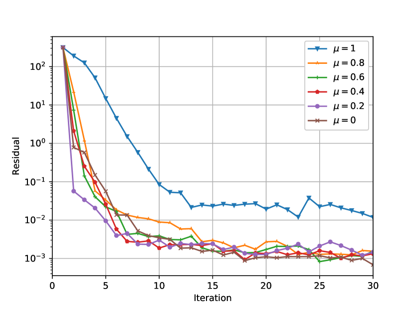
(a) Test 1 (Trajectory: 8)

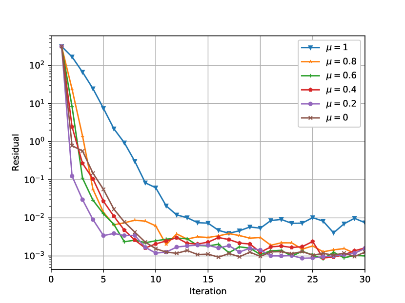
(b) Test 1 (Trajectory: 10)

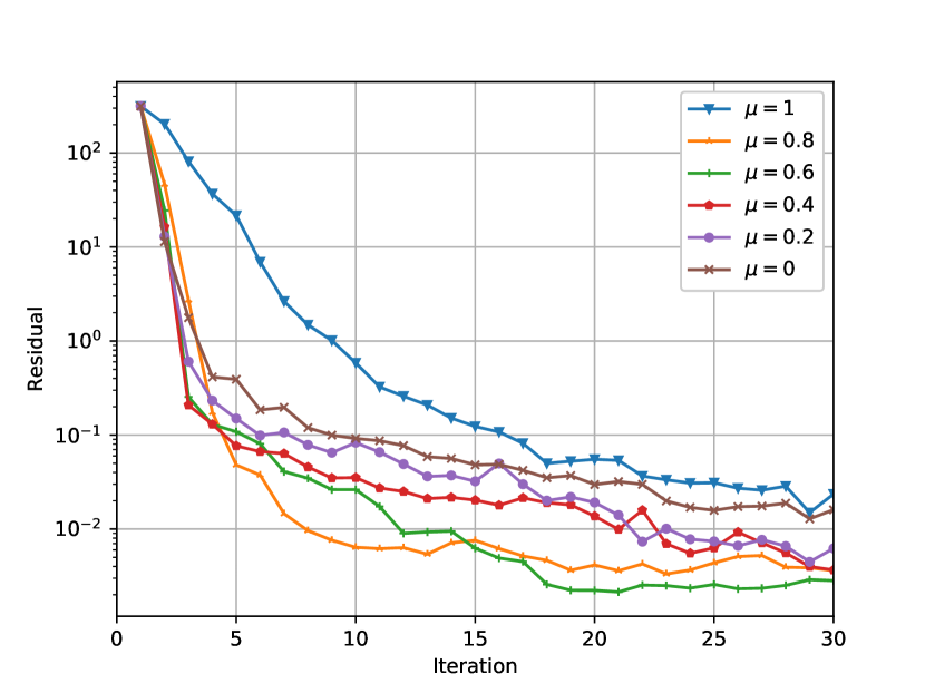
(c) Test 2 (Trajectory: 6)

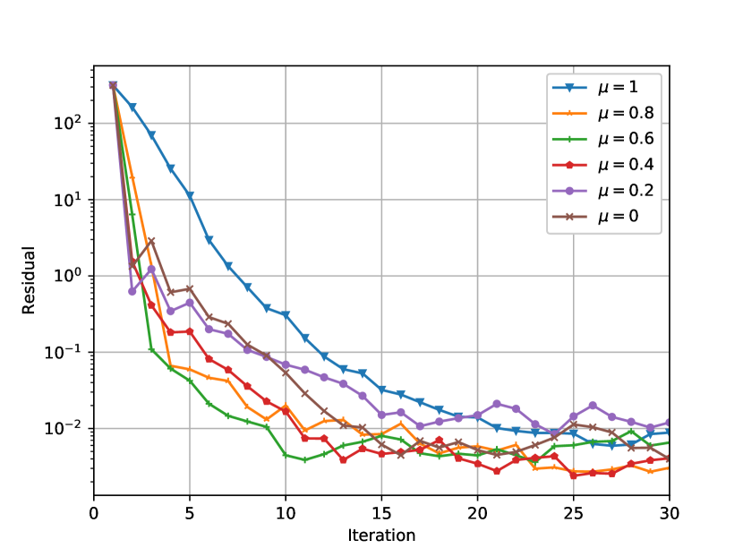
(d) Test 2 (Trajectory: 8)

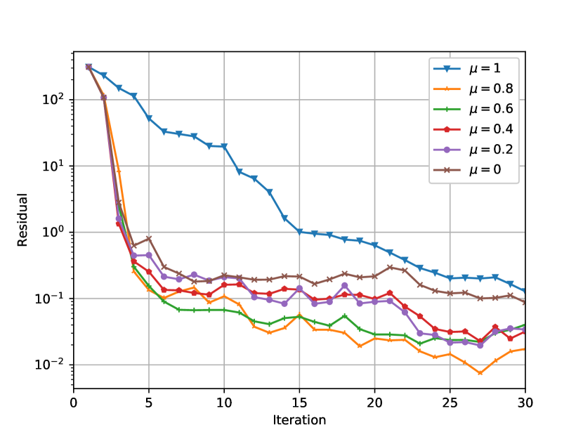
(e) Test 3 (Trajectory: 4)

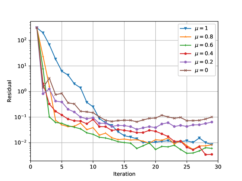
(f) Test 3 (Trajectory: 10)

Figure 1: Error (HJB residual) vs policy iteration for various $\mu$.

Experiment 2. The purpose of Experiment 2 is to test the performance of the methods when the training process is not exact. Recall that in Experiment 1, we have set the maximum steps in training process as a sufficiently large number 1000. Here, we limit this maximum training step to the range $10\sim 200$. A small maximum training step means less accuracy in fitting the value function. For each test, the algorithm is run up to 120 policy iterations and the number of characteristics trajectories is fixed as a relatively small number $N=5$ now.

	$\mu$	Train step
		10	50	100	150	200
T1	$1.0$	1.476	Diverge	Diverge	1.03$\times 10^{-2}$	1.55$\times 10^{-2}$
	$0.8$	4.36$\boldsymbol{\rm\times 10^{-4}}$	4.46$\boldsymbol{\rm\times 10^{-4}}$	4.58$\boldsymbol{\rm\times 10^{-4}}$	4.57$\boldsymbol{\rm\times 10^{-4}}$	4.51$\boldsymbol{\rm\times 10^{-4}}$
	$0.6$	6.12$\rm\times 10^{-4}$	6.18$\rm\times 10^{-4}$	6.25$\rm\times 10^{-4}$	6.25$\rm\times 10^{-4}$	6.45$\rm\times 10^{-4}$
	$0.4$	7.02$\rm\times 10^{-4}$	7.10$\rm\times 10^{-4}$	7.14$\rm\times 10^{-4}$	7.12$\rm\times 10^{-4}$	7.30$\rm\times 10^{-4}$
	$0.2$	7.62$\rm\times 10^{-4}$	7.66$\rm\times 10^{-4}$	7.68$\rm\times 10^{-4}$	7.70$\rm\times 10^{-4}$	7.84$\rm\times 10^{-4}$
	$0.0$	8.04$\rm\times 10^{-4}$	8.02$\rm\times 10^{-4}$	8.08$\rm\times 10^{-4}$	8.10$\rm\times 10^{-4}$	8.19$\rm\times 10^{-4}$
T2	$1.0$	0.146	Diverge	Diverge	Diverge	Diverge
	$0.8$	2.93$\boldsymbol{\rm\times 10^{-4}}$	2.80$\boldsymbol{\rm\times 10^{-4}}$	2.84$\boldsymbol{\rm\times 10^{-4}}$	2.88$\boldsymbol{\rm\times 10^{-4}}$	2.92$\boldsymbol{\rm\times 10^{-4}}$
	$0.6$	4.13$\rm\times 10^{-4}$	3.88$\rm\times 10^{-4}$	3.83$\rm\times 10^{-4}$	3.83$\rm\times 10^{-4}$	3.82$\rm\times 10^{-4}$
	$0.4$	4.42$\rm\times 10^{-4}$	4.51$\rm\times 10^{-4}$	4.46$\rm\times 10^{-4}$	4.46$\rm\times 10^{-4}$	4.36$\rm\times 10^{-4}$
	$0.2$	4.56$\rm\times 10^{-4}$	4.87$\rm\times 10^{-4}$	4.57$\rm\times 10^{-4}$	4.70$\rm\times 10^{-4}$	4.76$\rm\times 10^{-4}$
	$0.0$	4.83$\rm\times 10^{-4}$	5.15$\rm\times 10^{-4}$	4.98$\rm\times 10^{-4}$	5.07$\rm\times 10^{-4}$	2.23$\rm\times 10^{-3}$
T3	$1.0$	7.47$\times 10^{-2}$	Diverge	5.91$\rm\times 10^{-4}$	8.48$\rm\times 10^{-4}$	1.21$\times 10^{-2}$
	$0.8$	3.53$\rm\times 10^{-4}$	2.32$\boldsymbol{\rm\times 10^{-4}}$	2.36$\boldsymbol{\rm\times 10^{-4}}$	2.45$\rm\times 10^{-4}$	2.61$\boldsymbol{\rm\times 10^{-4}}$
	$0.6$	3.39$\boldsymbol{\rm\times 10^{-4}}$	3.06$\rm\times 10^{-4}$	3.17$\rm\times 10^{-4}$	3.35$\rm\times 10^{-4}$	3.19$\rm\times 10^{-4}$
	$0.4$	4.31$\rm\times 10^{-4}$	3.59$\rm\times 10^{-4}$	3.56$\rm\times 10^{-4}$	3.65$\rm\times 10^{-4}$	7.77$\rm\times 10^{-4}$
	$0.2$	4.53$\rm\times 10^{-4}$	3.96$\rm\times 10^{-4}$	4.07$\rm\times 10^{-4}$	1.08$\boldsymbol{\rm\times 10^{-4}}$	1.05$\rm\times 10^{-2}$
	$0.0$	5.09$\rm\times 10^{-4}$	4.20$\rm\times 10^{-4}$	8.48$\times 10^{-3}$	5.20$\times 10^{-3}$	8.31$\rm\times 10^{-3}$

Table 2: Error (HJB residual) for various $\mu$ when the training steps change.

The average HJB residuals of the last 20 policy iterations are reported in Table 2 to measure the accuracy. This table shows that $\mu=1$ has the worst performance in Test 1 and Test 2 and neither $\mu=1$ nor $\mu=0$ can perform well in Test 3. It is confirmed that the setting of $\mu$ strictly between $0$ and $1$ is more robust to incomplete training and also has better performance in accuracy. We can also see from this table that there is in general no necessity to use strict stopping criteria for training the interpolation for $\widehat{\Phi}_{Q}$. Even a small training step $10$ with a choice $\mu\in(0,1)$ can have the same final accuracy as the large training step $200$.

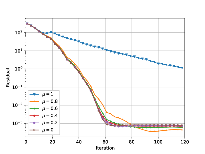
(a) Test 1 (Train step: 10)

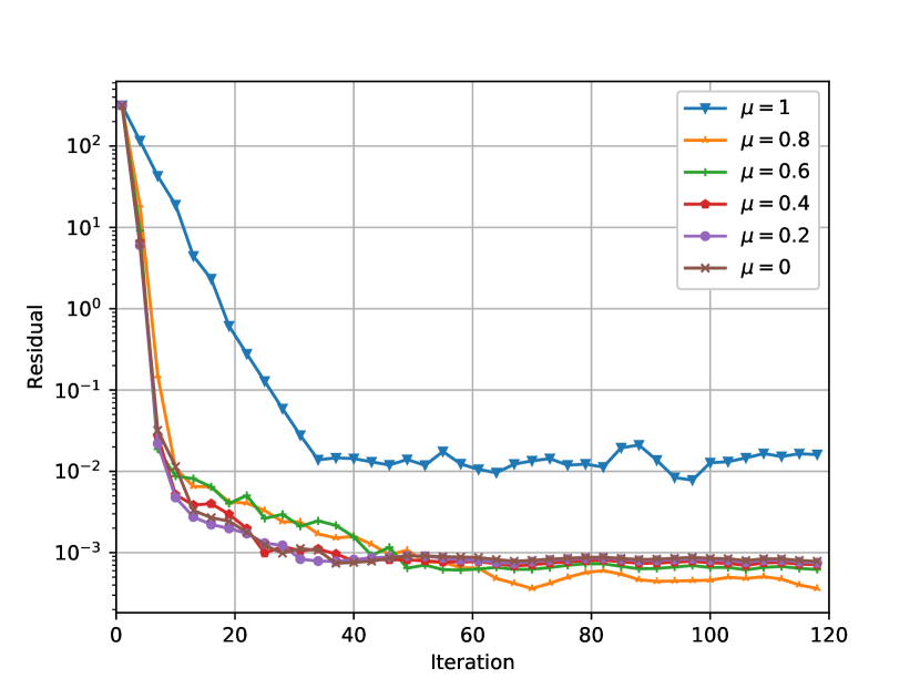
(b) Test 1 (Train step: 200)

(c) Test 2 (Train step: 10)

(d) Test 2 (Train step: 200)

(e) Test 3 (Train step: 10)

(f) Test 3 (Train step: 200)

Figure 2: Error (HJB residual) vs policy iteration for various $\mu$. The trajectory number is 5.

Fig. 2 shows the convergence of the policy iteration at different $\mu$ values. We see that again for all three tests, $\mu=1$ which corresponds to the policy iteration with only the value function gives the slowest decay of error among all $\mu$ tests. For other values of $\mu<1$, the performances of reducing the error are basically similar and all outperform the case of $\mu=1$.

In summary, for the toy model of linear-quadratic problem, we have conducted many numerical tests to show the advantage of our formulation of using the value-gradient data in training the value function: it improves the convergence of the policy iteration and shows much better robustness for a limited amount of data and a limited number of training steps.

5.2 Cart-pole balancing

Cart-pole balancing task is a 4-dim nonlinear case [2]. The physical model of this task includes a car, a pole and a ball. The ball is connected to one end of the pole and the other end of the pole is fixed to the car. The pole can rotate around the end fixed to the car, while the car is put on a flat surface, being able to move left or right. The aim of this task is to balance the pole in the upright vertical direction.

The state variable has four dimensions: the angular velocity of the ball, denoted by $\omega$; the included angle of the pole and the vertical direction, denoted by $\psi\in[-\pi,\pi]$; the velocity of the car, denoted by $v$; the position of the car, denoted by $z$. The control of this problem is the force applied to the car, denoted by $F$.

The control problem is to let $\psi$ be as small as possible. To eliminate the translation invariant in the horizontal position, we also want $z$ to be small. So we aim to minimize $-\cos(\psi)$ and $|z|^{2}$ with the following cost function

$$J(u)=\int_{0}^{\infty}e^{-\rho t}\left(-\cos(\psi(t))+\eta|z(t)|^{2}\right)\text{d}t$$

with $\rho=5$ and $\eta=0.2$ and subject to the dynamical system

$$\left\{\begin{aligned} &\dot{\omega}=\frac{g\sin\psi+\frac{\left(\mu_{c}\operatorname{sgn}(v)-F-ml\omega^{2}\sin\psi\right)\cos\psi}{m+m_{c}}-\frac{\mu_{p}\omega}{ml}}{l\left(\frac{4}{3}-\frac{m}{m+m_{c}}\cos^{2}\psi\right)}\\ &\dot{\psi}=\omega\\ &\dot{v}=\frac{F+ml\left(\omega^{2}\sin\psi-\dot{\omega}\cos\psi\right)-\mu_{c}\operatorname{sgn}(v)}{m+m_{c}}\\ &\dot{z}=v\\ &\omega(0)=\omega_{0},\psi(0)=\psi_{0},v(0)=v_{0},z(0)=z_{0}\end{aligned}\right.$$

where $m$ is the mass of the ball, $m_{c}$ is the mass of the car, $l$ is the length of the pole, $g$ is the gravitational constant. A constraint is imposed to the control: $|F|\leq F_{max}$, $F_{max}\geq 0$ is the largest control we can have. These hyper-parameters are set to be

$$m=0.1,\ l=0.5,\ m_{c}=1,\ \mu_{c}=5\times 10^{-4},\ \mu_{p}=2\ \times 10^{-6},\ F_{max}=10.$$

The state variable is $x=(\omega,\psi,v,z)\in\mathbb{R}^{4}$ with $\psi\in[-\pi,\pi)$. The value function is approximated by neural network with radial basis function ($n=50$ modes). Totally, there are $(2d+1)n=450$ parameters to learn. We compute the value function on the domain $\Omega=[-2\pi,2\pi]\times[-\pi,\pi]\times[-0.5,0.5]\times[-2.4,2.4]$. So the initial values of the characteristics $X_{0}^{(n)}$ are uniformly sampled from $\Omega$. But the characteristics are computed in the whole space with sufficiently long time until $e^{-\rho t}\Phi(X(t))$ and $e^{-\rho t}\lambda(X(t))$ are both sufficiently small. Error of the numerical solution $\widehat{\Phi}_{\theta}$ is measured by the HJE residual calculated on $N_{p}=10000$ points uniformly sampled from $\Omega$:

(5.53) $$\begin{split}error=\frac{1}{N_{p}}\sum^{N_{p}}_{j=1}\Big{\|}\rho\hat{\Phi}_{\theta}\left(x^{(j)}\right)-g&\left(x^{(j)},a^{*}\left(x^{(j)}\right)\right)\cdot\nabla\hat{\Phi}_{\theta}\left(x^{(j)}\right)-l\left(x^{(j)},a^{*}\left(x^{(j)}\right)\right)\Big{\|},\end{split}$$

where $x^{(j)}$ is the $j$-th data point.

To better evaluate the performance, we introdue the ”successful roll-up”: in a 20 second simulation ($T=20$), if

• $|\psi(t)|<\pi/4$ lasts for at least 10 seconds;

• $|z(t)|<10$ for all $t\in[0,T]$.

Then we call this run a ”successful roll-up”.

The initial condition for measuring the successful roll-up numbers are $(\omega(0),\psi(0),\ \$ $v(0)=0,z(0)=0)$ with 100 pairs of $(\omega(0),\psi(0))$ from the $10\times 10$ mesh grid of $[-2\pi,2\pi)\times[-\pi,\pi).$

We conduct the same two experiments as in the Linear-quadratic problem for this case which test the performance under insufficient data or incomplete training.

Experiment 1. In Experiment 1, we study how insufficient amount of characteristics data will affect the performance. Specifically, we test the performance of trajectory numbers of 2, 5 and 10 while the training for the supervised learning to minimize the loss $L(\theta)$ takes a fixed number of 50 ADAM steps. Fewer trajectories mean less amount of labelled data for the method of characteristics.

	$\mu$	Number of trajectories
		2	5	10
Residual	$1.0$	2.088	0.844	0.934
	$0.8$	0.696	0.281	0.100
	$0.6$	0.450	0.169	0.117
	$0.4$	0.441	0.147	0.091
	$0.2$	0.181	0.113	0.082
	$0.0$	0.166	0.124	0.094
Successful roll-up	$1.0$	14.85	19.25	12.30
	$0.8$	10.65	25.10	60.8
	$0.6$	27.10	25.15	38.65
	$0.4$	11.05	39.25	44.20
	$0.2$	9.30	40.95	50.45
	$0.0$	20.95	44.95	55.00

Table 3: The error (HJE residual) and the number of successful roll-ups for different $\mu$ when the trajectory number $N$ changes in the cart-pole balancing task. The train step is 100.

Table 3 shows the results when $\mu$ varies for each test. For each given $N$, the collection of $N$ initial states are the same at different $\mu$ for consistent comparison. The average residual error of the last 20 iterations is reported in the table. For each setting, the best residual is highlighted in bold symbols and the worst residual is emphasised in italics. From the table, we can see that $\mu=1$ performs the worst in all cases. In fact, a huge improvement can be observed in the residual and successful roll-up number when the gradient information is used. Also, this table confirms that with the number of characteristics increasing, the final accuracy of the numerical value functions always gets better and better since more labelled data are provided.

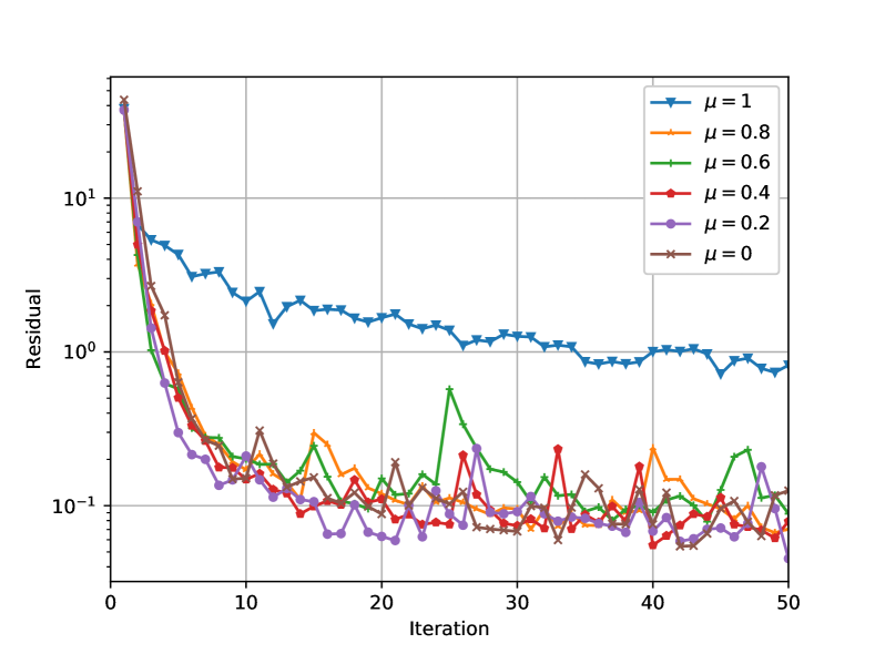
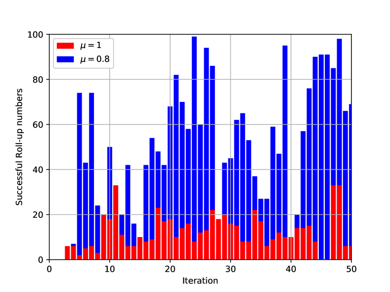
Figure 3: Residual and the successful roll-ups with trajectory number of 10 and train step of 100 in the cart-pole task.

To investigate the effect of $\mu$ on the decay of the error, we plot the residual error during the policy iteration in Fig. 3. This figure clearly demonstrates that $\mu=1$ has the slowest convergence among all $\mu$ we tested, and we can find that adding even a small portion of the loss for the value-gradient, i.e., $\mu<1$, can improve the convergence. Also, we plot the successful roll-up number of $\mu=1$ compared with $\mu=0.8$ at each iteration. It can be seen that value-gradient significantly improves the performance.

Experiment 2. The purpose of Experiment 2 is to test the performance of the methods when the training process is not sufficiently long. In this experiment, the train steps 50, 100, 150 and 200 are tested. A small training step means less accuracy in fitting the value function. The trajectory number is now fixed as 10.

	$\mu$	Train step
		50	100	150	200
Residual	$1.0$	1.355	0.934	0.500	0.471
	$0.8$	0.260	0.100	0.151	0.155
	$0.6$	0.175	0.117	0.092	0.097
	$0.4$	0.096	0.091	0.105	0.103
	$0.2$	0.106	0.082	0.094	0.080
	$0.0$	0.130	0.094	0.070	0.083
Successful roll-up	$1.0$	13.75	12.30	28.55	30.00
	$0.8$	58.25	60.80	41.45	35.80
	$0.6$	28.05	38.65	16.50	35.55
	$0.4$	56.40	44.20	36.50	35.75
	$0.2$	61.65	50.45	35.30	47.00
	$0.0$	21.85	55.00	49.30	54.10

Table 4: The error (HJE residual) and the number of successful roll-ups for different $\mu$ when training steps change in the cart-pole balancing task. The trajectory number is 10.

As shown in Table 4, the accuracy gets quite remarkable improvements as long as the value-gradient is included in the formulation. The successful roll-ups also show a better performance for $\mu<1$, particularly when the number of trajectories increases.

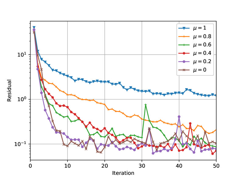
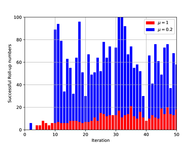
Figure 4: Residual and the successful roll-ups with trajectory number of 10 and train step of 50 in the cart-pole task.

Fig. 4 shows the residual and successful roll-ups with respect to the policy iteration for different $\mu$ values. As expected, choosing $\mu<1$ gets these results considerably improved.

5.3 Advertising process

This example is a 3-dim nonlinear case from [43, 19]. The three dimensions of the states are the advertising stimulus level $A$, the adaptation level $\overline{A}$ and sales $S$. We are aiming at finding the optimal advertising effort $u$ that maximize the cost function

$$J(u)=\int_{0}^{\infty}e^{-\rho t}(\pi S(t)-u(t))\mathrm{d}t,$$

subject to the dynamic system

$$\left\{\begin{aligned} &\dot{A}=u-\delta A,A(0)=A_{0}\\ &\dot{\overline{A}}=\zeta(A-\overline{A}),\overline{A}(0)=\overline{A}_{0}\\ &\dot{S}=v\ln(A+1)-\alpha S+\overline{w}\max\{0,A-\overline{A}\},S(0)=S_{0}\end{aligned}\right.$$

where $\delta$ is a constant proportional depreciation rate, $\zeta>0$ represents the relative weight of more rescent levels of advertising capital, $\alpha$ denotes the proportion of customers switching to other brands per unit time, $\pi$ is the gross profit per unit sold and $\overline{w}$ and $v$ are constants. The control $u$ has upper bound and lower bound $0\leq u\leq\overline{u}$. All the hyper-parameters are set to:

$$\overline{u}=2,\delta=0.5,\zeta=1,v=0.5,\alpha=0.1,\overline{w}=0.5,\pi=0.5$$

The value function is parametrized as a family of radial basis functions with 60 modes. We also conduct two experiments on this problem as previous examples. The total number of policy iteration is 200.

Experiment 1. In Experiment 1, trajectory numbers of 2, 5, 10 are tested. The training step is fixed to 50. Table 5 records the average HJB residual (5.53) of the last 40 iterations of the 200 policy iterations. As is shown in the table, $\mu=1$ has the worst residual among all. Fig. 5 demonstrates the residual with respect to the policy iteration number. $\mu\in[0,1)$ converges faster and performs better than $\mu=1$.

$\mu$	Number of trajectories
	2	5	10
$1.0$	0.0627	0.0429	0.0286
$0.8$	0.0373	0.0265	0.0180
$0.6$	0.0506	0.0251	0.0180
$0.4$	0.0511	0.0205	0.0193
$0.2$	0.0447	0.0237	0.0106
$0.0$	0.0417	0.0107	0.0080

Table 5: The HJB residual for different $\mu$ in advertise process task Experiment 2. Smaller residuals are better results. The best value for each trajectory number is highlighted in bold symbols and the worst is marked in italics. The training step is 50.

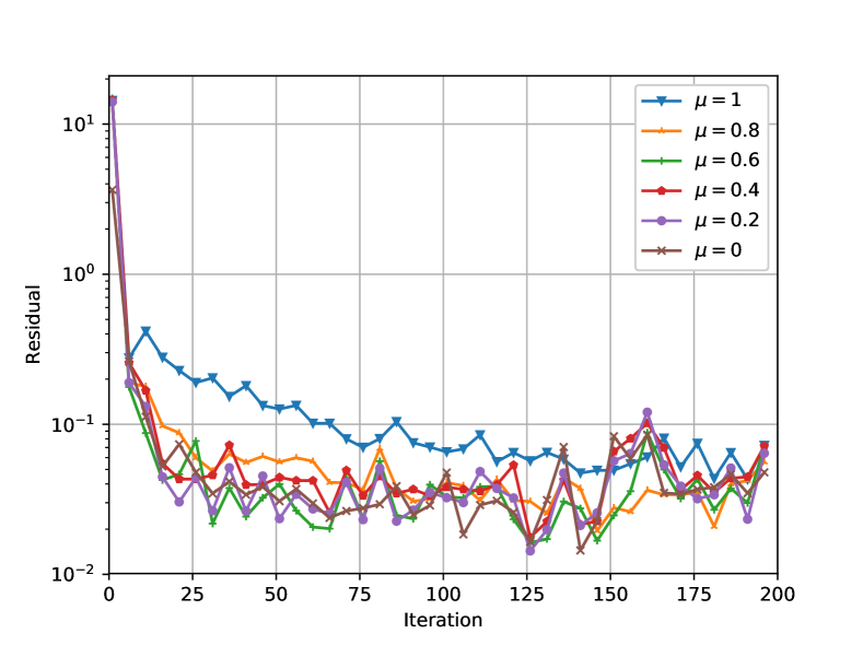
(a) Trajectory Number: 2

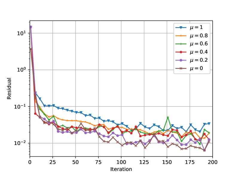
(b) Trajectory Number: 10

Figure 5: Residual during the 200 policy iteration for various $\mu$ in the advertise process task. The trajectory numbers are 2 and 10 and the training step is 50.

Experiment 2. In Experiment 2, we test the training step of 25, 50, 75, 100. Table 6 records the residual error and Fig. 6 demonstrates the residual with respect to the policy iteration number. It can be concluded that using a mixture of value and value gradient works better than using value only.

$\mu$	Number of train steps
	25	50	75	100
$1.0$	0.04098	0.0429	0.03651	0.03772
$0.8$	0.03134	0.0265	0.02986	0.02800
$0.6$	0.02844	0.0251	0.02578	0.02731
$0.4$	0.02149	0.0205	0.02107	0.03110
$0.2$	0.02111	0.0237	0.01160	0.03220
$0.0$	0.01632	0.0107	0.01101	0.02522

Table 6: The HJB residual for different $\mu$ in advertise process task Experiment 2. Smaller residuals are better results. The best value for each train step selection is highlighted in bold symbols and the worst is marked in italics. The trajectory number is 5.

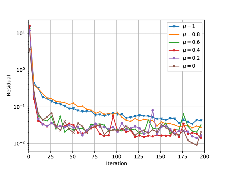
(a) Train step: 25

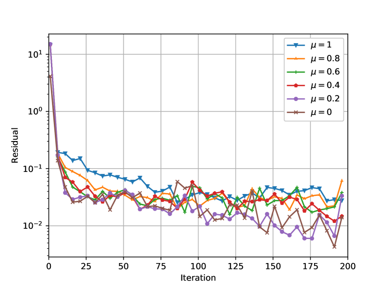
(b) Train step: 75

Figure 6: Residual during the policy iteration with training steps of 25 and 75 in advertise process task. The trajectory number is 5.

To conclude the above experiment, we have performed the numerical tests by changing the amount of characteristics data and the training steps, which are two important factors in practical computation. By comparing the performance measured by the HJE residual as the error and the successful roll-ups as the robustness, we find that these numerical results consistently show the outperformance when using the characteristics data both from the value and the value-gradient functions. Although the four tested values of $\mu=0.2,0.4,0.6,0.8$ between $0$ and $1$ always beat the traditional method at $\mu=1$, the optimal value $\mu$ actually varies on the specific settings and the difference among these four values for the performance is marginal.

6 Conclusion

Based on the system of PDEs for the value-gradient functions we derived in this paper, we develop a new policy iteration framework, called PI-lambda, for the numerical solution of the value function for the optimal control problems. We show the convergence property of this iterative scheme under Section 2.1. The system of PDEs for the value-gradient functions $\lambda(x)$ is closed since it does not involve the value function $\Phi(x)$ at all, so one could in principle use neural networks only for $\lambda$. This is distinctive from many existing methods based on value function (e.g. [22]). The system for $\lambda$ is also essentially decoupled and shares the same characteristics ODE with the generalized HJE. By simulating characteristics curves in parallel for the state variable by any classic ODE solver (like Runge-Kutta method), both the value $\Phi$ and the value-gradient functions $\lambda$ on each characteristics curve can be computed. Equipped with any state-of-the-art function representation technique and the large-scale minimization techniques from supervised learning, these labelled data can be generalized to the whole space to deal with high dimensional problems. Policy iteration has the computational convenience to simulate the characteristics equations only forward in time, instead of solving any boundary-value problem for optimal trajectories directly as in [25, 28, 33]. Policy iteration is also convenient when Hamiltonian minimization has no analytical expression. The learning procedure of supervised learning in our method is not new, and it has been applied, for example in [40, 25, 32], to combine the losses from the policy data, the value function data and the value-gradient data altogether. Our distinction from these works is to formulate the co-state variable as the gradient function $\lambda(x)$ of the state, not a function of the time $\lambda(t)$ in PMP.

The generalization to the finite horizon control problem on $[0,T]$ is straightfoward: to replace $\rho\lambda(x)$ by $-\partial_{t}\lambda(t,x)$ in equation (3.18) and add the transversality condition $\lambda(T,x)=\nabla_{x}h(T,x)$ when there is a terminal cost $h(T,x(T))$. The main algorithm in this paper based on the policy iteration, PI-lambda, is still applicable and our main theorem (Theorem 3.5) can be easily generalized.

Some practical computational issues which are not fully discussed here include the choice of the initial policy $a^{(0)}$, the number of trajectories $N$ and their initial locations $\left\{X_{0}\right\}$. For the initial policy, it should be chosen conservatively to stabilize the dynamics. For the characteristics curves, $N$ may be changed from iteration to iteration, and adaptive sampling for the initial states is a good issue for further exploration [32]. If a neural network is used, the network structure is also an important practical issue [33].

An obvious question to address in future is how to formulate the equations of $\lambda$ for the stochastic optimal control so as to leverage the similar benefit of our algorithm here for the deterministic control problem. One may consider the splitting method in [8].

References

- [1] A. Alla, M. Falcone, and D. Kalise, An efficient policy iteration algorithm for dynamic programming equations, SIAM Journal on Scientific Computing, 37 (2015), pp. A181–A200, https://doi.org/10.1137/130932284.
- [2] S. Barto, Neuronlike adaptive elements that can solve difficult learning control problems, IEEE Transactions on Systems, Man, and Cybernetics, 13 (1983), pp. 834–846.
- [3] R. W. Bea, Successive Galerkin approximation algorithms for nonlinear optimal and robust control, International Journal of Control, 71 (1998), pp. 717–743, https://doi.org/10.1080/002071798221542.
- [4] R. W. Beard, G. N. Saridis, and J. T. Wen, Galerkin approximations of the generalized Hamilton-Jacobi-Bellman equation, Automatica, 33 (1997), pp. 2159–2177, https://doi.org/10.1016/S0005-1098(97)00128-3.
- [5] R. W. Beard, G. N. Saridis, and J. T. Wen, Approximate solutions to the time-invariant Hamilton–Jacobi–Bellman equation, Journal of Optimization Theory and Applications, 96 (1998), pp. 589–626.
- [6] R. Bellman, A Markovian Decision Process, Indiana University Mathematics Journal, 6 (1957), pp. 679–684, https://doi.org/10.1512/iumj.1957.6.56038.
- [7] R. Bellman, Dynamic Programming, Princeton University Press, 1957.
- [8] A. Bensoussan, Splitting up method in the context of stochastic PDE, in Stochastic Partial Differential Equations and Their Applications, B. L. Rozovskii and R. B. Sowers, eds., Berlin, Heidelberg, 1992, Springer Berlin Heidelberg, pp. 22–31.
- [9] A. Bensoussan, Estimation and Control of Dynamical Systems, Interdisciplinary Applied Mathematics, Springer International Publishing, 2018.
- [10] A. Bensoussan, Y. Li, D. Phan Cao Nguyen, M.-B. Tran, S. C. P. Yam, and X. Zhou, Machine Learning and Control Theory, to apper in NUMERICAL CONTROL: PART B, volume 24 of Handbook of Numerical Analysis, Elsever, (2020), https://arxiv.org/abs/2006.05604.
- [11] D. P. Bertsekas, Dynamic Programming and Optimal Control, Vol. I, 2nd Ed., Athena Scientific, Belmont, MA, 2001.
- [12] D. P. Bertsekas, Reinforcement Learning and Optimal Control, Athena Scientific, Belmont, MA, 2019.
- [13] Y. T. Chow, J. Darbon, S. Osher, and W. Yin, Algorithm for overcoming the curse of dimensionality for time-dependent non-convex hamilton–jacobi equations arising from optimal control and differential games problems, Journal of Scientific Computing, 73 (2017), pp. 617–643, https://doi.org/10.1007/s10915-017-0436-5.
- [14] Y. T. Chow, J. Darbon, S. Osher, and W. Yin, Algorithm for overcoming the curse of dimensionality for certain non-convex Hamilton–Jacobi equations, projections and differential games, Annals of Mathematical Sciences and Applications, 3 (2018), pp. 369–403.
- [15] Y. T. Chow, W. Li, S. Osher, and W. Yin, Algorithm for Hamilton–Jacobi equations in density space via a generalized Hopf formula, Journal of Scientific Computing, 80 (2019), pp. 1195–1239.
- [16] J. Darbon and S. Osher, Algorithms for overcoming the curse of dimensionality for certain Hamilton–Jacobi equations arising in control theory and elsewhere, Research in the Mathematical Sciences, 3 (2016), pp. 1–26.
- [17] W. E, J. Han, and A. Jentzen, Algorithms for solving high dimensional PDEs: From nonlinear Monte Carlo to machine learning, arXiv preprint arXiv:2008.13333, (2020).
- [18] M. Falcone and R. Ferretti, Semi-Lagrangian approximation schemes for linear and Hamilton—Jacobi equations, SIAM, 2013.
- [19] G. Feichtinger, R. F. Hartl, S. P. Sethi, G. Feichtinger, R. F. Hartl, and S. P. Sethi, Dynamic Optimal Control Models in Advertising : Recent Developments Linked references are available on JSTOR for this article : Dynamic Optimal Control Models in Advertising : Recent Developments, 40 (1994), pp. 195–226.
- [20] W. Fleming and H. Soner, Controlled Markov Processes and Viscosity Solutions, Stochastic Modelling and Applied Probability, Springer New York, 2006.
- [21] W. H. Fleming and R. W. Rishel, Deterministic and Stochastic Optimal Control, Stochastic Modelling and Applied Probability, Springer New York, 1975, https://doi.org/10.1007/978-1-4612-6380-7.
- [22] J. Han, A. Jentzen, and W. E, Solving high-dimensional partial differential equations using deep learning, Proceedings of the National Academy of Sciences, 115 (2018), pp. 8505–8510, https://doi.org/10.1073/pnas.1718942115.
- [23] M. B. Horowitz, A. Damle, and J. W. Burdick, Linear Hamilton-Jacobi-Bellman equations in high dimensions, in 53rd IEEE Conference on Decision and Control, 2014, pp. 5880–5887, https://doi.org/10.1109/CDC.2014.7040310.
- [24] R. A. Howard, Dynamic programming and Markov processes, The Technology Press of M.I.T., Cambridge, Mass.; John Wiley & Sons, Inc., New York-London, 1960.
- [25] D. Izzo, E. Öztürk, and M. Märtens, Interplanetary transfers via deep representations of the optimal policy and/or of the value function, in Proceedings of the Genetic and Evolutionary Computation Conference Companion, GECCO ’19, New York, NY, USA, 2019, Association for Computing Machinery, p. 1971–1979, https://doi.org/10.1145/3319619.3326834.
- [26] D. Kalise and K. Kunisch, Polynomial approximation of high-dimensional Hamilton-Jacobi-Bellman equations and applications to feedback control of semilinear parabolic PDES, SIAM Journal on Scientific Computing, 40 (2018), pp. A629–A652, https://doi.org/10.1137/17M1116635.
- [27] W. Kang and L. Wilcox, A causality free computational method for HJB equations with application to rigid body satellites, in AIAA Guidance, Navigation, and Control Conference, 2015, p. 2009.
- [28] W. Kang and L. C. Wilcox, Mitigating the curse of dimensionality: sparse grid characteristics method for optimal feedback control and HJB equations, Computational Optimization and Applications, 68 (2017), pp. 289–315, https://doi.org/10.1007/s10589-017-9910-0.
- [29] D. P. Kingma and J. Ba, Adam: A method for stochastic optimization, arXiv preprint arXiv:1412.6980, (2014).
- [30] E. C. Lawrence, Partial differential equations (second edition), American Mathematical Society, 2010.
- [31] A. T. Lin, Y. T. Chow, and S. J. Osher, A splitting method for overcoming the curse of dimensionality in Hamilton–Jacobi equations arising from nonlinear optimal control and differential games with applications to trajectory generation, Communications in Mathematical Sciences, 16 (2018), https://doi.org/10.4310/cms.2018.v16.n7.a9.
- [32] T. Nakamura-Zimmerer, Q. Gong, and W. Kang, Adaptive deep learning for high-dimensional hamilton–jacobi–bellman equations, SIAM Journal on Scientific Computing, 43 (2021), pp. A1221–A1247, https://doi.org/10.1137/19M1288802.
- [33] T. Nakamura-Zimmerer, Q. Gong, and W. Kang, Qrnet: Optimal regulator design with lqr-augmented neural networks, IEEE Control Systems Letters, 5 (2021), pp. 1303–1308, https://doi.org/10.1109/LCSYS.2020.3034415.
- [34] S. Osher and J. A. Sethian, Fronts propagating with curvature-dependent speed: Algorithms based on Hamilton-Jacobi formulations, Journal of Computational Physics, 79 (1988), pp. 12–49.
- [35] M. Oster, L. Sallandt, and R. Schneider, Approximating the stationary Hamilton-Jacobi-Bellman equation by hierarchical tensor products, arXiv: 1911.00279, (2019).
- [36] L. S. Pontryagin, Mathematical Theory of Optimal Processes, CRC Press, 1987.
- [37] M. L. Puterman and S. L. Brumelle, On the convergence of policy iteration in stationary dynamic programming, Mathematics of Operations Research, 4 (1979), pp. 60–69, https://doi.org/10.1287/moor.4.1.60.
- [38] B. Recht, A Tour of Reinforcement Learning: The View from Continuous Control, Annual Review of Control, Robotics, and Autonomous Systems, 2 (2019), pp. 253–279, https://doi.org/10.1146/annurev-control-053018-023825.
- [39] R. S. Sutton and A. G. Barto, Reinforcement Learning: An Introduction, Adaptive Computation and Machine Learning series, MIT Press, 2018.
- [40] D. Tailor and D. Izzo, Learning the optimal state-feedback via supervised imitation learning, Astrodynamics, 3 (2019), pp. 361–374, https://doi.org/10.1007/s42064-019-0054-0.
- [41] Y.-H. R. Tsai, L.-T. Cheng, S. Osher, and H.-K. Zhao, Fast sweeping algorithms for a class of Hamilton–Jacobi equations, SIAM Journal on Numerical Analysis, 41 (2003), pp. 673–694, https://doi.org/10.1137/S0036142901396533.
- [42] J. N. Tsitsiklis, Efficient algorithms for globally optimal trajectories, in Proceedings of 1994 33rd IEEE Conference on Decision and Control, vol. 2, 1994, pp. 1368–1373 vol.2.
- [43] T. Vienna, Theory and Methodology ADPULS in continuous time, 34 (1988), pp. 171–177.