violetrgb0.5, 0.0, 0.5 lukescolorrgb0.8, 0.33, 0.0 applegreenrgb0.55, 0.71, 0.0

Strong parametric dispersive shifts in a statically decoupled multi-qubit cavity QED system

Abstract

Cavity quantum electrodynamics (QED) with in-situ tunable interactions is important for developing novel systems for quantum simulation and computing.Rauschenbeutel et al. (1999); Allman et al. (2010); Srinivasan et al. (2011); Potts et al. (2016); Vaidya et al. (2018); Suleymanzade et al. (2020) The ability to tune the dispersive shifts of a cavity QED system provides more functionality for performing either quantum measurements or logical manipulations. Here, we couple two transmon qubits to a lumped-element cavity through a shared dc-SQUID.Zakka-Bajjani et al. (2011); Lu et al. (2017) Our design balances the mutual capacitive and inductive circuit components so that both qubits are highly decoupled from the cavityLu et al. (2017), offering protection from decoherence processesWhittaker et al. (2014); Zhang et al. (2017). We show that by parametrically drivingZakka-Bajjani et al. (2011); Allman et al. (2014); Lu et al. (2017) the SQUID with an oscillating flux it is possible to independently tune the interactions between either of the qubits and the cavity dynamically. The strength and detuning of this cavity-QED interaction can be fully controlled through the choice of the parametric pump frequency and amplitude. As a practical demonstration, we perform pulsed parametric dispersive readout of both qubits while statically decoupled from the cavity. The dispersive frequency shifts of the cavity mode follow the expected magnitude and sign based on a simple theory that is supported by a more thorough theoretical investigationXiao et al. (2021). This parametric approach creates a new tunable cavity QED framework for developing quantum information systems with various future applications, such as entanglement and error correction via multi-qubit parity readoutRoch et al. (2014); Riste et al. (2013); Andersen et al. (2019), state and entanglement stabilizationLu et al. (2017); Kimchi-Schwartz et al. (2016); Doucet et al. (2020), and parametric logical gatesReagor et al. (2018); Noguchi et al. (2018).

Cavity QED has become a backbone for some of the leading quantum information processing systems. In particular, systems based on superconducting circuits, so called circuit QED systemsBlais et al. (2004); Koch et al. (2007), provide a promising platform for realizing a practical quantum information processing unit. These systems usually rely on a static coupling between the qubit and cavity. Schuster et al. (2005); Houck et al. (2008). In order to overcome the drawbacks in these systems, such as frequency crowding, additional decoherence, and always-on interactions, systems have been developed that use flux tunable elements Allman et al. (2010); Srinivasan et al. (2011); Allman et al. (2014); Whittaker et al. (2014); Zhang et al. (2017) to set the coupling strength between a qubit and cavity via a static magnetic field. Tunable couplers have led to improved coherence and fast, high-fidelity two-qubit entangling gates Chen et al. (2014) and qubit measurements have been performed while avoiding decoherence caused by unwanted interactions with the cavity. Whittaker et al. (2014); Zhang et al. (2017)

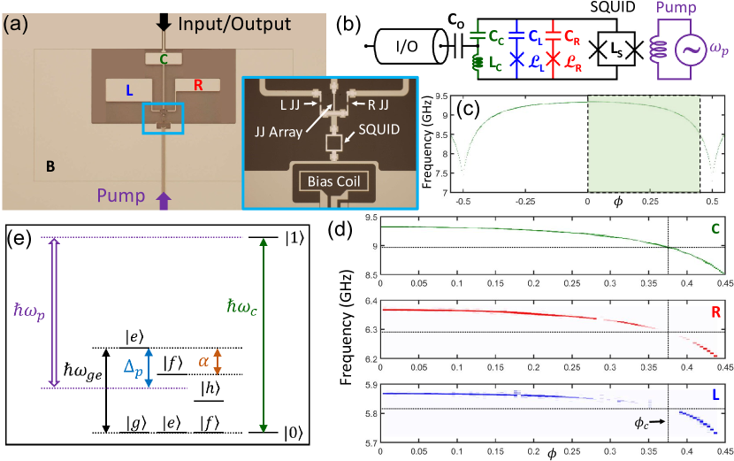
Figure 1: (Color online) (a) Optical micrograph of a tunable circuit QED system. (b) Schematic diagram of the system including the three elements: cavity mode (C), Left transmon (L), and Right transmon (R). The parametric flux drive is applied through a shared dc-SQUID coupler. (c) Periodic cavity spectrum. (d) Frequency of the three resonant modes, C, R, and L as a function of the flux bias $\phi=\Phi/\Phi_{0}$. (e) Energy scale diagram showing the relationship between defined quantities, see the main text for the details.

One difficulty with systems that rely on a tunable static flux is that the frequency of all the coupled elements are usually strongly dependent on the applied flux.Allman et al. (2010); Srinivasan et al. (2011); Allman et al. (2014); Whittaker et al. (2014); Zhang et al. (2017) Therefore, the tuning of the cavity QED parameters also involves strong manipulation of the frequency of the cavity QED elements. This can be a disadvantage as each element experiences a phase shift when their resonant frequency is adjusted. When performing quantum operations, these shifts must usually be accounted for or corrected. In addition, when many elements share the same frequency space, flux tuning can lead to unwanted frequency collisions and unwanted coupled interactions, complicating the system operation.

Parametric interactions represent an alternative coupling mechanism with many benefits. Zakka-Bajjani et al. (2011); Allman et al. (2014); Chen et al. (2014); Roushan et al. (2017) When used in cavity QED-type systems where the parametric pump is resonant with the difference frequency between the qubit and cavity, one can perform rapid swap operations between the coupled systems with rates that are directly proportional to the amplitude of the pump drive. Zakka-Bajjani et al. (2011); Allman et al. (2014) These type of interactions can be important for cavity photon state manipulation, photon-photon interference, and performing gate operations. Zakka-Bajjani et al. (2011); Nguyen et al. (2012); Allman et al. (2014); Rosenblum et al. (2018). However, parametric operations within the dispersive regime, where the coupled systems do not exchange energy, can also be very useful. Three-dimensional cavity QED systems have taken advantage of four-wave mixing through a single Josephson junction of a capacitively coupled transmonRosenblum et al. (2018) to provide for dynamically adjustable dispersive shifts. Rosenblum et al. (2012) Parametric coupling between Qubit-cavity systems can also useful for stabilizing the state of a single transmon qubit Lu et al. (2017) or the entanglement of multi-qubit systems Doucet et al. (2020); et al. (2021a).

In this work, we describe a two-transmon qubit cavity QED system whereby the interactions with a single cavity mode coupled to an input/output microwave feedline are tuned through the use of a parametric flux drive applied to a shared dc-SQUID coupler. We investigate in detail the dispersive frequency shifts on the cavity mode induced by inserting a single photon in one of the qubits as a function of the parametric pump’s drive frequency and amplitude. We find that these shifts can be well described by a simple model that is a parametric generalization of the standard dispersive formulas introduced for circuit QED with a transmon. Koch et al. (2007) Moreover, we observe experimentally some interesting new features at higher pump amplitudes that can be explained by higher order corrections from the absorption of multiple photons between the transmon’s energy levels. Xiao et al. (2021) In addition, this system also allows parametric interactions between the two qubits, independent of the cavity, for applying parametric entangling gatesReagor et al. (2018); Noguchi et al. (2018) or between all three systems for the stabilization of arbitrarily entangled two-qubit statesKimchi-Schwartz et al. (2016); Doucet et al. (2020), as will be described in future worket al. (2021b, c, a).

With a nearly 0.5 GHz separation between the qubits, the parametric dispersive shifts of the cavity due to either qubit can be independently controlled by selectively applying a specific pump frequency. Both the amplitude and sign of these shifts can be controlled by adjusting the pump amplitude and frequency. Remarkably, we can dynamically access both positive and negative relative detunings allowing us access to all three distinct dispersive regions Koch et al. (2007); Xiao et al. (2021), beyond the usual ac Stark effect expected for a two-level atom. Therefore, along with the commonly used negative dispersive shifts, we can also generate large, positive shifts that hitherto only occurred in the “straddling regime” of static circuit QED Koch et al. (2007), where the cavity frequency must sit between the first two qubit transition frequencies, $\omega_{ge}$ and $\omega_{ef}$. In this work, by dynamically driving the coupler, a “parametric straddling regime” has been discovered even with the cavity frequency nearly 3 GHz above both qubits. This results from the fact that the parametric generalization of the qubit-cavity detuning $\Delta_{p}$, the parametric coupling strength $g_{p}$, and either transmon anharmonicity $\alpha$ satisfy the necessary straddling regime conditions, making it fully accessible. Koch et al. (2007); Xiao et al. (2021)

As a practical demonstration of parametrically controlled dispersive shifts, we show that we can pulse “on” these shifts in-time in order to measure either qubit, or apply them simultaneously to perform a joint readout of the two-qubit states Roch et al. (2014); Riste et al. (2013); Andersen et al. (2019). One unique design feature of our parametric strategy is that each qubit can be protected Srinivasan et al. (2011); Zhang et al. (2017) from the cavity during its logical operations. Only when it is time to measure the qubit do we turn on the parametric interactions generating large dispersive shifts to enable qubit state readout. To this end, we characterize the residual static dispersive shift between the qubits and the cavity as a function of the flux in the SQUID coupler. Furthermore, by injecting photons into the cavity, we can witness the elimination of additional qubit dephasing even in the presence of photon shot noise in the cavity. Zhang et al. (2017) These results set the stage for future work. Because these parametric dispersive shifts can be applied simultaneously, with adjustable strength and sign, and add linearly, we can explore the construction of multi-qubit parity measurements, useful for measuring error syndromes and performing quantum error correction. Roch et al. (2014); Riste et al. (2013); Andersen et al. (2019)

Our circuit, as shown in Fig. 1(a)–(b), has been constructed to largely cancel static coupling between both qubits and the cavity Allman et al. (2010, 2014); Lu et al. (2017), so that parametric couplings dominate the interactions (see Supplemental Material (SM)). Each frequency is partially defined by the three top capacitor plates ($C$, $L$, and $R$) for the three lumped-element resonators. The left ($L$) and the right ($R$) transmons each have nominally the same Josephson junction with critical current $I_{o}\approx 36$ nA that defines the Josephson energy $E_{J}=I_{o}\Phi_{o}/2\pi$. The central cavity ($C$) uses a series array of 7 larger junctions (each with $I_{oC}\approx 15I_{o}$) to form a nearly linear inductance $L_{C}$. The dc-SQUID coupler, formed by a small loop that includes two Josephson junctions with critical currents $I_{o1}=I_{o2}\approx 15I_{o}$, shares current between all three elements with the large common electrode, or bottom plate $B$. We have purposefully chosen the orientation and distance between the three top capacitor plates in order for their mutual capacitive coupling to cancel the mutual inductive coupling of the SQUID at a particular static flux bias $\phi_{c}=\Phi_{c}/\Phi_{o}$, which we refer to as the “cancellation flux”, where $\Phi_{o}=h/2e$ is the magnetic flux quantum. At this flux, the static coupling between all three elements should in-principle be zero, leaving them uncoupled and thus independent. Of course, achieving this condition perfectly is challenging (see SM).

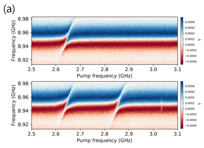
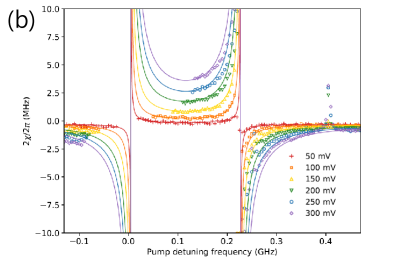
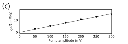
Figure 2: (Color online) (a) A typical full cavity spectrum while sweeping the pump frequency $\omega_{p}$. The upper and lower panel shows the phase of the cavity signal with the R transmon in state $|g\rangle_{R}$ and $|e\rangle_{R}$, respectively. (b) The parametrically induced dispersive shifts as a function of the pump detuning frequency, $\Delta_{pR}=\omega_{p}-|\Delta_{R}|$, at various calibrated pump amplitudes: 50 (red), 100 (orange), 150 (yellow), 200 (green), 250 (blue), and 300 mV (purple), respectively. The solid lines are fits for the data from the theory. See the text for the details. (c) Parametric $g_{pR}$ as a function of pump amplitude.

Standard circuit QED theory Blais et al. (2004); Koch et al. (2007) describes the interaction between an individual transmon $k=L,R$, with anharmonicity $\alpha_{k}<0$, and a cavity $C$ as (with $\hbar=1$),

$$H=\sum_{k=\{L,R\}}\omega_{k}q_{k}^{\dagger}q_{k}+\frac{\alpha_{k}}{2}(q_{k}^{\dagger}q_{k})^{2}+\omega_{C}c^{\dagger}c+H_{Ik},$$ (1)

with the interaction Hamiltonian is given by,

$$H_{Ik}=g_{sk}(q_{k}+q_{k}^{\dagger})(c+c^{\dagger}),$$ (2)

where $q_{k}^{\dagger}$ ($q_{k}$) is the creation (annihilation) operator of the $k$th transmon mode, $c^{\dagger}$ ($c$) corresponds to the same for the cavity mode, $\omega_{k}$ and $\omega_{C}$ are the frequencies of the $k$th transmon and cavity, respectively, and $g_{sk}\equiv g_{sk}(\phi)$ is the SQUID-tunable, total static coupling rate Allman et al. (2010, 2014); Whittaker et al. (2014); Lu et al. (2017) between the $k$th transmon and the cavity. We will define the states $|g\rangle_{k}$, $|e\rangle_{k}$ and $|f\rangle_{k}$ as the first three eigenstates of the $k$th transmon, respectively, while the cavity states are referred to as $|n\rangle$ for photon numbers $n=0,1,2\cdots$.

In the dispersive regime of cavity QED Blais et al. (2004); Koch et al. (2007); Boissonneault et al. (2009), when $g_{sk}\ll|\Delta_{k}|$ where $\Delta_{k}=\omega_{k}-\omega_{C}$ is the detuning between the $k$th transmon and $g_{sk}$ is the static coupling strength, the interaction Hamiltonian in Eq. (2) simply becomes $H_{Ik}=2\chi_{sk}q_{k}^{\dagger}q_{k}c^{\dagger}c$. In this regime, the qubit and cavity both experience a total dispersive frequency shift $2\chi_{sk}$ depending on the energy state of the other element of the system. In our case, the flux-tunable static dispersive strength $\chi_{sk}(\phi)=(g_{sk}^{2}(\phi)/\Delta_{k})(\alpha_{k}/(\alpha_{k}+\Delta_{k}))$. Koch et al. (2007) Here, the separation between the cavity transition frequencies when the $k$th qubit is in $|g\rangle_{k}$ and $|e\rangle_{k}$ is $2\chi_{sk}$. At a flux bias far from the cancellation flux, the residual static coupling $g_{sk}$ is predominantly capacitive (when $\phi<\phi_{c}$) or inductive (when $\phi>\phi_{c}$). We can easily perform qubit spectroscopy when $\chi_{sk}$ is relatively large, however the spectrum fades away on either side of the cancellation flux as $g_{sk}$ becomes significantly reduced (see Fig. 1(d)).

The frequencies of all the resonant modes are periodic as a function of $\phi$ (as shown for the cavity in Fig. 1(c)). In Fig. 1(d), we shown all the spectra over nearly a half-a-period in $\phi$. At $\phi=0$, the maximum qubit frequencies are about 5.9 GHz ($L$) and 6.4 GHz ($R$), while the maximum cavity frequency is about 9.4 GHz. The cavity is coupled to a co-planar waveguide feedline for the input and output of microwave photons leading to a typical total decay rate of $\kappa/2\pi\approx 10$ MHz, which is flux dependent (see SM). The transmon anharmonicities are also flux dependent (see SM), with average values of $\alpha_{L}/2\pi\approx-180$ MHz and $\alpha_{R}/2\pi\approx-220$ MHz.

We can access a new, rich set of dynamics by moving beyond the static interactions typical of standard cavity QED systems, by driving the tunable coupler with a sinusoidal flux modulation in addition to a static flux bias, $\phi(t)=\phi_{m}\sin(\omega_{p}t)+\phi_{s}$. This parametric pump drive then modifies the interaction strength in Eq. (2), leading to the following coupling terms written in an interaction frame w.r.t. the free Hamiltonian Allman et al. (2014),

$$H_{pk}=-i\sum_{k=\{L,R\}}g_{pk}\left(e^{i\omega_{p}t}-e^{-i\omega_{p}t}\right)(q_{k}c^{\dagger}e^{i\Delta_{k}t}+{\rm h.c.}),$$ (3)

where we have ignored the sum frequency terms for the regime under consideration, i.e. $\omega_{p}$ near the difference frequency $|\Delta_{k}|$. In general, the pump frequency can be detuned by $\Delta_{pk}$, $\omega_{p}=|\Delta_{k}|+\Delta_{pk}$, in order to sweep between parametrically-induced resonant-type ($\Delta_{pk}\ll g_{pk}$) and dispersive-type ($\Delta_{pk}\gg g_{pk}$) interactions, corresponding to the $|g\rangle_{k}\rightarrow|e\rangle_{k}$ transition and the cavity mode. This can been seen by measuring the full spectrum of the cavity mode for a fixed pump amplitude when $\omega_{p}\approx|\Delta_{R}|$, as shown in the upper panel of Fig. 2(a). Notice the avoided crossing is clearly visible with a coupling strength, $2g_{pR}/2\pi\approx 10$ MHz. This data was taken when starting from $|g\rangle_{R}$. If, after a $\pi$-pulse, we start from $|e\rangle_{R}$ and take the same spectrum in the presence of the pump tone, we can see (lower panel of Fig. 2(a)) another avoided crossing from the $|e\rangle_{R}\rightarrow|f\rangle_{R}$ transition becoming resonant with the cavity mode. Notice that this splitting is centered about $\Delta_{pR}=-\alpha_{R}>0$. This behavior is also seen for higher level transmon transitions Xiao et al. (2021), which agrees with Eq. 4, and these results have been repeated successfully for the $L$ transmon as well (see SM).

In order to fully characterize the additional dispersive shifts imparted to the cavity by the presence of the parametric pump, we measure the full cavity spectrum for various calibrated pump amplitudes (see SM) while sweeping $\omega_{p}$. We take two data sets for each pump amplitude, one starting from $|g\rangle_{R}$ and one starting from $|e\rangle_{R}$, like the data sets shown in Fig. 2(a)). By comparing the two results, we can extract the full dispersive shifts as shown in Fig. 2(b). For the smallest pump amplitude and largest $\Delta_{pR}$, notice that the dispersive shift is nearly zero. This is because we have chosen $\phi\approx\phi_{c}$, as discussed below. In general, the parametric dispersive shifts simply add to the static shifts Xiao et al. (2021) (see SM for data at more bias points).

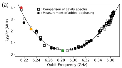
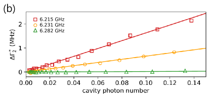
Figure 3: (Color online) (a) The static dispersive shift $2\chi_{s}/2\pi$ as a function of the R transmon frequency. For red open squares, the dispersive shift was measured by comparing the cavity response with the R transmon in either state $|g\rangle_{R}$ or $|e\rangle_{R}$. For blue filled circles, the dispersive shift was extracted by measuring additional dephasing $\Gamma_{\phi R}$ while driving the cavity to a weak coherent state, see the main text for the details. The solid line represents a polynomial fit to the data. (b) Additional dephasing as a function of the average photon number $\bar{n}$ at three different flux biases where the R tranmon frequencies are 6.215 (red square), 6.231 (yellow circle), and 6.282 GHz (green triangle), respectively. Solid lines are a linear fit for the data.

In order to gain physical intuition, the parametric interactions can be analyzed in a rotating frame defined w.r.t. the pump frequency $\omega_{p}$. For an arbitrary pump detuning $\Delta_{pk}$, this necessitates including contributions from both positive and negative frequency components, as well as those corresponding to the sum and difference frequencies. Xiao et al. (2021) However, for sufficiently small $\Delta_{pk}$, in this rotating frame, the form of Eq. (3) becomes analogous to the static dispersive case with the identification $g_{sk}\rightarrow g_{pk}$ and $\Delta_{k}\rightarrow\Delta_{pk}$. Koch et al. (2007) We can even extend this picture to include higher transmon levels (see SM),

$$\chi_{pk}=\frac{g_{pk}^{2}}{\Delta_{pk}}\left[\frac{\alpha_{k}}{(\alpha_{k}+\Delta_{pk})}-\frac{\Delta_{pk}}{(2\alpha_{k}+\Delta_{pk})}-\frac{\Delta_{pk}}{(3\alpha_{k}+\Delta_{pk})}\cdots\right],$$ (4)

This simplified expression describes the data quite well and the extracted values for $g_{pR}$ are plotted in Fig. 2(c), which clearly shows a linear dependence on the pump amplitude. Moreover, at a fixed amplitude, $g_{pR}\propto\sqrt{(d\omega_{R}/d\phi)(d\omega_{C}/d\phi)}$ agrees with predictions Zakka-Bajjani et al. (2011); Allman et al. (2014) based on the slope of the qubit and cavity at the cancellation flux $\phi_{c}$ (see SM). At larger powers, however, we find a very interesting peak in the data that occurs at $\Delta_{pR}=-2\alpha_{R}$. This corresponds to a pump-mediated two-photon transition between the first- and third-excited states of the transmon Xiao et al. (2021). Such features are described by quartic-order contributions to dispersive shift $\chi_{pk}$ and exhibit an even lineshape in pump detuning, thus providing a means to distinguish them from the lower-order quadratic features that lead to an odd lineshape (see Fig. 2(b)).

As a simple demonstration of the usefulness of programmable dispersive shifts in this new parametric circuit-QED framework, we next describe qubit measurements near the cancellation flux. One drawback when working with static cavity QED systems is that a persistent dispersive interaction can lead to two decoherence processes, enhanced energy relaxation Houck et al. (2008), reducing the qubit relaxation time $T_{1}$, and additional dephasing Schuster et al. (2005), reducing the qubit dephasing time $T_{2}$. Although the qubit and the cavity are detuned from each other, the qubit’s decay rate $1/T_{1}$ is enhanced by an additional Purcell factor of $(g/\Delta)^{2}\kappa$ due to radiative decay through the coupled cavity mode. Whereas qubit dephasing occurs because the dispersive interaction also modifies the qubit’s frequency depending on the photon occupancy within the cavity. The additional dephasing is given by the rate $\Gamma_{n}=8\bar{n}\kappa\chi_{s}^{2}/(\kappa^{2}+4\chi_{s}^{2})$, where $\bar{n}$ is the average number of (coherent state) photons in the cavity. Schuster et al. (2005); Gambetta et al. (2006) These decoherence mechanisms can be reduced in circuit QED systems by using Purcell filters Reed et al. (2010) (increases $T_{1}$ only) or eliminating the total qubit-cavity coupling Allman et al. (2010); Srinivasan et al. (2011); Allman et al. (2014); Zhang et al. (2017) (increases both $T_{1}$ and $T_{2}$). One difficulty with the second approach is that once $g_{sk}\approx 0$, it is not possible to measure the qubit dispersively, unless the qubit has hidden degrees of freedom still coupled to the cavity Zhang et al. (2017) or you rapidly tune-up $g_{sk}(\phi)$ through a flux shift pulse in time for the measurement Whittaker et al. (2014).

Alternatively, our circuit allows us to minimize $g_{sk}$ by setting $\phi=\phi_{c}$, while still enabling dispersive qubit readout by applying a parametric pump tone with a given amplitude and frequency $\omega_{p}$, as described above (see Fig. 2). Ideally, when $\chi_{s}\propto g_{sk}^{2}\rightarrow 0$, both qubits are completely decoupled statically from the cavity. In Fig. 3(a), we show the static dispersive shift $\chi_{sR}$ (and $g_{sR}$, see SM) as a function of the R transmon frequency. For the open square, we directly measured the dispersive shift by comparing the cavity response with the R transmon in either state $|g\rangle_{R}$ or $|e\rangle_{R}$. The solid line comes from a polynomial fit that matches our predictions based on a circuit model (see SM). In Fig. 3(b), we also measured additional dephasing $\Gamma_{\phi R}$ of the R transmon while driving the cavity with a weak coherent state with an average photon number $\bar{n}$ for each flux bias. Schuster et al. (2005); Zhang et al. (2017) Crucially, the measurement of the R transmon near the cancellation flux required using a parametric tone to perform the dispersive readout. We see that $\Gamma_{\phi R}$ scales linearly with $\bar{n}$ as expected Schuster et al. (2005); Gambetta et al. (2006) and the slope significantly diminishes as the bias approaches the cancellation flux. From this data, and knowing $\kappa$, we can extract $\chi_{sR}$ (and $g_{sR}$) for each bias (see SM). This result is plotted as filled circles in Fig. 3(a) and agrees well with the direct measurements. These results were also performed on the L transmon with similar results (see SM). The minimum value for $\chi_{sR}/2\pi$ ($\chi_{sL}/2\pi$) was $300$ kHz ($150$ kHz), which was limited by the nonlinearity of the SQUID coupler itself (see SM).

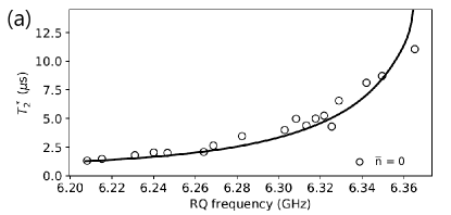
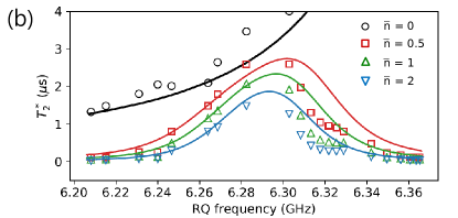
Figure 4: (Color online) (a) The phase coherence time $T^{*}_{2}$ as a function of the R transmon frequency when $\bar{n}\approx 0$. The solid black line is a fit based on the dominant dephasing coming from flux noise. (b) Comparison of $T^{*}_{2}$ in the presence of coherent cavity photons with $\bar{n}=$ 0.5 (square), 1 (up-triangle), and 2 (down-triangle). The solid lines are predictions based the measurement, see the main text for the details.

Finally, we can demonstrate that the qubits are protected from photon shot noise in the cavity by comparing the additional dephasing just discussed ($\bar{n}\neq 0$) with the background dephasing when $\bar{n}\approx 0$. Zhang et al. (2017) In Fig. 4(a), we plot the phase coherence time $T^{*}_{2}$ of the R qubit obtained by measuring Ramsey oscillations as a function of its frequency. The solid line is a fit to the data assuming that the dominant source of background dephasing is coming from flux noise in the coupler, which is proportional to the slope $d{\omega_{R}(\phi)}/d\phi$ of the modulation curve of R transmon frequency with flux (see Fig. 1). In Fig. 4(b), we compare this result with $T^{*}_{2}$ of the R transmon in the presence of photon shot noise for $\bar{n}=$0, 0.5, 1, and 2. Here, the solid lines are predictions based on the directly measured values for $\chi_{sR}$ as a function of flux and the average value of $\kappa$ over whole range of flux considered in the measurement. As we can see, the R transmon is protected from shot noise in the cavity near $\phi=\phi_{c}$, where the dephasing is dominated by flux noise in the coupler. Similar results were found for the L transmon as well (See SM).

In conclusion, we have developed a unique tunable cavity QED system that allows for in-situ dynamic control over the interaction between a qubit and a cavity by applying a parametric tone. We demonstrated that this can be accomplished with a two-qubit system, that can also allow for a fully adjustable joint two-qubit measurement. We operated our two-transmon circuit QED system in the dispersive regime and explored the dynamic control of parametrically induced dispersive cavity shifts from either transmon. By varying the sign and size of these shifts with the amplitude and frequency of the parametric pump, we have unlocked a “parametric straddling regime” and verified a simple theoretical model that generalizes this behavior in the rotating frame. As a practical application, we pulsed the parametric pump simultaneously with a readout tone, and with a proper choice for the amplitude and frequency, we performed dispersive qubit readout on both transmons. Due to our unique circuit design that minimizes static coupling to the cavity, the transmons were protected during local logical operations from photon shot noise in the cavity. We believe that this new tunable cavity QED framework will open up a novel paradigm for controlling light-matter interactions by providing a unique functionality along with qualitatively new features that are not supported by static circuit-QED setups.

This work was partially performed under the following financial assistance award 70NANB18H006 from U.S. Department of Commerce, National Institute of Standards and Technology. T.N., Z.X.,E.D.,L.R.,L.G. and A.K. received support from the Department of Energy under grant DE-SC0019461.

References

- Rauschenbeutel et al. (1999) A. Rauschenbeutel, A. G. Nogues, S. Osnaghi, P. Bertet, M. Brune, J. M. Raimond, and S. Haroche, Phys. Rev. Lett. 83, 5166 (1999).
- Allman et al. (2010) M. Allman, F. Altomare, J. Whittaker, K. Cicak, D. Li, A. Sirois, J. Strong, J. Teufel, and R. Simmonds, Phys. Rev. Lett. 104, 177004 (2010).
- Srinivasan et al. (2011) S. J. Srinivasan, A. J. Hoffman, J. M. Gambetta, and A. A. Houck, Phys. Rev. Lett. 106, 083601 (2011).
- Potts et al. (2016) C. A. Potts, A. Melnyk, H. Ramp, M. H. Bitarafan, D. Vick, L. J. LeBlanc, J. P. Davis, and R. G. DeCorby, Appl. Phys. Lett. 108, 041103 (2016).
- Vaidya et al. (2018) V. D. Vaidya, Y. Guo, R. M. Kroeze, K. E. Ballantine, A. J. Kollár, J. Keeling, and B. L. Lev, Phys. Rev. X 8, 011002 (2018).
- Suleymanzade et al. (2020) A. Suleymanzade, A. Anferov, M. Stone, R. K. Naik, A. Oriani, J. Simon, and D. Schuster, Appl. Phys. Lett. 116, 104001 (2020).
- Zakka-Bajjani et al. (2011) E. Zakka-Bajjani, F. Nguyen, M. Lee, L. R. Vale, R. W. Simmonds, and J. Aumentado, Nature Physics 7, 599 (2011).
- Lu et al. (2017) Y. Lu, S. Chakram, N. Leung, N. Earnest, R. K. Naik, Z. Huang, P. Groszkowski, E. Kapit, J. Koch, and D. I. Schuster, Phys. Rev. Lett. 119, 150502 (2017).
- Whittaker et al. (2014) J. D. Whittaker, F. C. S. da Silva, M. S. Allman, F. Lecocq, K. Cicak, A. J. Sirois, J. D. Teufel, J. Aumentado, and R. W. Simmonds, Phys. Rev. B 90, 024513 (2014).
- Zhang et al. (2017) G. Zhang, Y. Liu, J. J. Raftery, and A. A. Houck, npj Quantum Information 3, 1 (2017).
- Allman et al. (2014) M. Allman, J. Whittaker, M. Castellanos-Beltran, K. Cicak, F. da Silva, M. DeFeo, F. Lecocq, A. Sirois, J. Teufel, J. Aumentado, and R. Simmonds, Phys. Rev. Lett. 112, 123601 (2014).
- Xiao et al. (2021) Z. Xiao, E. Doucet, T. Noh, R. W. Simmonds, L. Ranzani, L. C. G. Govia, and A. Kamal, Arxiv: 2103.09260 (2021).
- Roch et al. (2014) N. Roch, M. E. Schwartz, F. Motzoi, C. Macklin, R. Vijay, A. W. Eddins, A. N. Korotkov, K. B. Whaley, M. Sarovar, and I. Siddiqi, Phys. Rev. Lett. 112, 170501 (2014).
- Riste et al. (2013) D. Riste, M. Dukalski, C. A. Watson, G. de Lange, M. J. Tiggelman, Y. M. Blanter, K. W. Lehnert, R. N. Schouten, and L. DiCarlo, Nature 502, 350 (2013).
- Andersen et al. (2019) C. K. Andersen, A. Remm, S. Lazar, S. Krinner, J. Heinsoo, J.-C. Besse, M. Gabureac, A. Wallraff, and C. Eichler, npj Quantum Information 5, 69 (2019).
- Kimchi-Schwartz et al. (2016) M. E. Kimchi-Schwartz, L. Martin, E. Flurin, C. Aron, M. Kulkarni, H. E. Tureci, and I. Siddiqi, Phys. Rev. Lett. 116, 240503 (2016).
- Doucet et al. (2020) E. Doucet, F. Reiter, L. Ranzani, and A. Kamal, Phys. Rev. Research 2, 023370 (2020).
- Reagor et al. (2018) M. Reagor, C. B. Osborn, N. Tezak, A. Staley, G. Prawiroatmodjo, M. Scheer, N. Alidoust, E. A. Sete, N. Didier, M. P. da Silva, E. Acala, J. Angeles, A. Bestwick, M. Block, B. Bloom, A. Bradley, C. Bui, S. Caldwell, L. Capelluto, R. Chilcott, J. Cordova, G. Crossman, M. Curtis, S. Deshpande, T. E. Bouayadi, D. Girshovich, S. Hong, A. Hudson, P. Karalekas, K. Kuang, M. Lenihan, R. Manenti, T. Manning, J. Marshall, Y. Mohan, W. O’Brien, J. Otterbach, A. Papageorge, J.-P. Paquette, M. Pelstring, A. Polloreno, V. Rawat, C. A. Ryan, R. Renzas, N. Rubin, D. Russel, M. Rust, D. Scarabelli, M. Selvanayagam, R. Sinclair, R. Smith, M. Suska, T.-W. To, M. Vahidpour, N. Vodrahalli, T. Whyland, K. Yadav, W. Zeng, and C. T. Rigetti, Science Advances 4, 2 (2018).
- Noguchi et al. (2018) A. Noguchi, A. Osada, S. Masuda, S. Kono, K. Heya, S. P. Wolski, H. Takahashi, T. Sugiyama, D. Lachance-Quirion, and Y. Nakamura, Phys. Rev. A 102, 062408 (2018).
- Blais et al. (2004) A. Blais, R.-S. Huang, A. Wallraff, S. M. Girvin, and R. J. Schoelkopf, Phys. Rev. A 69, 062320 (2004).
- Koch et al. (2007) J. Koch, T. M. Yu, J. Gambetta, A. A. Houck, D. I. Schuster, J. Majer, A. Blais, M. H. Devoret, S. M. Girvin, and R. J. Schoelkopf, Phys. Rev. A 76, 042319 (2007).
- Schuster et al. (2005) D. I. Schuster, A. Wallraff, A. Blais, L. Frunzio, R.-S. Huang, J. Majer, S. Girvin, and R. J. Schoelkopf, Phys. Rev. Lett. 94, 123602 (2005).
- Houck et al. (2008) A. A. Houck, J. A. Schreier, B. R. Johnson, J. M. Chow, J. Koch, J. M. Gambetta, D. I. Schuster, L. Frunzio, M. H. Devoret, S. M. Girvin, and R. J. Schoelkopf, Phys. Rev. Lett. 101, 080502 (2008).
- Chen et al. (2014) Y. Chen, C. Neill, P. Roushan, N. Leung, M. Fang, R. Barends, B. C. J. Kelly, B. C. Z. Chen, A. Dunsworth, E. Jeffrey, A. Megrant, J. Y. Mutus, P. J. J. O’Malley, C. M. Quintana, D. Sank, A. Vainsencher, J. Wenner, T. C. White, M. R. Geller, A. N. Cleland, and J. M. Martinis, Phys. Rev. Lett. 113, 220502 (2014).
- Roushan et al. (2017) P. Roushan, C. Neill, A. Megrant, Y. Chen, R. Babbush, R. Barends, B. Campbell, Z. Chen, B. Chiaro, A. Dunsworth, A. Fowler, E. Jeffrey, J. Kelly, E. Lucero, J. Mutus, P. J. J. O’Malley, M. Neeley, C. Quintana, D. Sank, A. Vainsencher, J.Wenner, T. White, E. Kapit, H. Neven, and J. Martinis, Nature Physics 13, 146 (2017).
- Nguyen et al. (2012) F. Nguyen, E. Zakka-Bajjani, R. W. Simmonds, and J. Aumentado, Phys. Rev. Lett. 108, 163602 (2012).
- Rosenblum et al. (2018) S. Rosenblum, Y. Gao, P. Reinhold, C. Wang, C. Axline, L. Frunzio, S. Girvin, L. Jiang, M. Mirrahimi, M. Devoret, and R. Schoelkopf, Nature Communications 9, 652 (2018).
- Rosenblum et al. (2012) S. Rosenblum, P. Reinhold, M. Mirrahimi, L. Jiang, L. Frunzio, and R. Schoelkopf, Science 361, 266 (2012).
- et al. (2021a) T. B. et al., Arxiv: in preparation (2021a).
- et al. (2021b) X. Y. J. et al., Arxiv: in preparation (2021b).
- et al. (2021c) X. Y. J. et al., Arxiv: in preparation (2021c).
- Boissonneault et al. (2009) M. Boissonneault, J. M. Gambetta, and A. Blais, Phys. Rev. A 79, 013819 (2009).
- Gambetta et al. (2006) J. Gambetta, A. Blais, D. I. Schuster, A. Wallraff, J. M. L. Frunzio, M. H. Devoret, S. M. Girvin, and R. J. Schoelkopf, Phys. Rev. A 74, 042318 (2006).
- Reed et al. (2010) M. D. Reed, B. R. Johnson, A. A. Houck, L. DiCarlo, J. M. Chow, D. I. Schuster, L. Frunzio, and R. J. Schoelkopf, Phys. Rev. Lett. 96, 203110 (2010).