Maximal Diversity and Zipf’s Law

Abstract

Zipf’s law describes the empirical size distribution of the components of many systems in natural and social sciences and humanities. We show, by solving a statistical model, that Zipf’s law co-occurs with the maximization of the diversity of the component sizes. The law ruling the increase of such diversity with the total dimension of the system is derived and its relation with Heaps’ law is discussed. As an example, we show that our analytical results compare very well with linguistics and population datasets.

Diversity is a central concept in ecology, economics, information theory, and other natural and social sciences. It can be quantified by diversity indices Jost (2006); Tuomisto (2010), such as (species) richness, the Gini-Simpson index or Boltzmann-Shannon entropy, which characterize the system under study from different angles. Loosely understanding the term, high diversity may represent an advantage in terms of resilience and performance. This is the case, for instance, in ecology, where well differentiated ecosystems are often (see, e.g., Ref. Ives and Carpenter (2007) for the debate on this topic) considered to be more stable Elton (1958); Tilman et al. (2006); Arese Lucini et al. (2020), and in economy as well: strong countries have a well diversified production Tacchella et al. (2012).

In most cases diversity is hindered by limiting factors. For an ecosystem the amount of energy and chemical components available does not allow an unbounded increase of the population. Similarly, the number of different items produced by an economy is limited by its strength. The diversity drift is therefore a complex optimization process.

Elaborating on that, in this Letter we take the aforementioned restrictions into account and, among the possible measures of diversity Jost (2006) we consider the richness index $D$, which turns out to be particularly suited for a quantitative description of such optimization tendency in many complex systems. Richness is a quantity that counts the number of different types which are present in a collection of items. For instance, the set of integers $\{3,7,1,9,0,1\}$ is richer than $\{3,2,3,7,7,2\}$, because there are 5 different figures in the former and only 3 in the latter. Every diversity measure can be rephrased in terms of Rényi Rényi et al. (1961) (or, equivalently, Tsallis Tsallis (1988)) entropies (see Ref. Jost (2006) and Supplemental Material (SM) Sup ). Notice, however, that the index $D$ alone is insensitive to the abundance of each type but only to their presence/absence.

We consider situations where types can be identified by quantitative labels $s$, as in the example above. $D$ is the richness of the collection of entities $\{s_{1},\dots,s_{N}\}$, with arbitrary $N$, but subjected to the additive constraint $S=\sum_{n=1}^{N}s_{n}$. Here $s_{n}$ represents the portion of the total resource $S$ assigned to the $n$-th entity of the ensemble, i.e. its size. Entities can be cities Gabaix (1999) of a country with total population $S$, distinct words Piantadosi (2014) occurring with absolute frequencies $\{s_{n}\}$ in a book of size $S$ or genes Furusawa and Kaneko (2003) expressed with abundances $\{s_{n}\}$ where $S$ is the total number of proteins synthesized in a cell.

These systems are instances where the Zipf’s law Zipf (1949); Newman (2005) is observed to hold. Other well known examples include Clauset et al. (2009) GDP of nations Cristelli et al. (2012), firm sizes Axtell (2001), species in taxa Willis and Yule (1922) and fragmentation processes Oddershede et al. (1993). If ranked according to their size $s$, components obey Zipf’s law when

$$s(r)\propto r^{-a},$$ (1)

where $r$ is the rank, with $a\simeq 1$. A representation in terms of the distribution of sizes Newman (2005); Corral et al. (2020) $p(s)\propto s^{-\tau}$, with $\tau=1+a^{-1}$, is better suited to our purposes. To explain Zipfian behavior many generative mechanisms have been proposed Simon (1955); Levy and Solomon (1996); Marsili and Zhang (1998); Ferrer-i-Cancho and Solé (2003); Tria et al. (2014); Corominas-Murtra et al. (2015); Mazzolini et al. (2018) and it has also been framed in a broader statistical perspective Mora and Bialek (2011); Marsili et al. (2013); Schwab et al. (2014). For instance, it has been shown to be associated to maximally informative samples in modeling complex systems Marsili et al. (2013); Cubero et al. (2019).

In this Letter we show that the maximization of the diversity index $D$ and the occurrence of Zipf’s law in the distribution of the component sizes $\{s_{n}\}$ are naturally related. This is achieved by deriving, in a statistical model, a diversity law that can be used to estimate the index $D$ of distributions of empirical data. We put our results to the test showing remarkable agreement with data for quantitative linguistics, taken from the Gutenberg English texts database Pro , and for urbanistics from the GeoNames database Geo . Finally, within our approach we also recover in a simple way the expression of Heaps’ law Heaps (1978); Lü et al. (2010) and discuss its relation with the diversity law. The fact that specifically $D$, among the possible diversity measures, is extremized, indicates the prominent role played by this quantity in the many and diverse natural phenomena described by the Zipf’s law and represents a different and perhaps profitable rationalization for its occurrence.

The model.—Consider sets of independent and identically distributed integer random variables $\{s_{n}\}$, sampled from a generic probability distribution $p(s)$. We call $s_{n}$ the size of the $n$-th component (or entity). $p(s)$ will be denoted as the bare distribution, since the effective (dressed) distribution of the $s_{n}$ is shaped by the presence of a global constraint $\sum_{n=1}^{N}s_{n}=S$, where $S$ is the total dimension of the system. $N$ is the fluctuating number of entities that, according to the particular extraction of the $\{s_{n}\}$, is needed to fulfill the constraint. The probability of a particular configuration $\mathcal{C}\equiv[\{s_{1},\ldots,s_{N}\};N]$ is given by

$$p_{S}(\{s_{1},\ldots,s_{N}\};N)=\frac{1}{Z_{S}}\prod_{n=1}^{N}p(s_{n})\delta_{\sum_{n=1}^{N}s_{n},S}\ ,$$ (2)

where the constraint is enforced by the Kronecker delta. The quantities $Z_{S}=\sum_{N=1}^{\infty}Z_{S}(N)$ and

$$Z_{S}(N)\equiv\sum_{s_{1}=1}^{S}\sum_{s_{2}=1}^{S}...\sum_{s_{N}=1}^{S}\prod_{n=1}^{N}p(s_{n})\delta_{\sum_{n=1}^{N}s_{n},S}\,\,\,$$ (3)

play the role of partition functions in an ensemble where $N$ is fluctuating or fixed, respectively. One obtains the probability of having a number $N$ of entities as $p_{S}(N)=Z_{S}(N)/Z_{S}$. The dressed probability of observing a size $s$ can be written using Eq. (3) as

$$p_{S}(s)=\frac{p(s)}{\sum_{N=1}^{\infty}N\ Z_{S}(N)}\sum_{N=1}^{\infty}N\ Z_{S-s}(N-1)\ ,$$ (4)

where the factor $N$ appears because we do not distinguish among components.

If $t_{s}$ is the number of times the value $s\in[1,S]$ is found in a given configuration ${\cal C}$, the diversity index $D$ (hereafter also referred to as simply diversity) is defined as

$$D=\sum_{s=1}^{S}\left(1-\delta_{t_{s},0}\right),$$ (5)

namely the number of different values assumed by the entities. The probability $p_{S}(D)$ of observing a certain value of $D$ is formally given in the SM Sup .

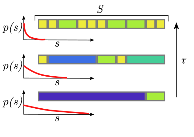
Figure 1: Pictorial representation of the problem. Power laws, $p(s)\sim s^{-\tau}$, are sketched with an increasing exponent $\tau$ (from bottom to top) alongside with relative typical realizations $\{s_{n}\}$. Entities of the same size are depicted as blocks of the same color and in all the cases they add up to $S$, the total length of the bar. For large values of $\tau$, most of the entities have small and similar sizes, resulting in a poor diversity $D$. In the other limit, small $\tau$, large sizes do get more probable but the total number of entities required to fill $S$ is smaller. Consequently, diversity is again small. The diversity is expected to be maximal for an intermediate value of $\tau$.

We are interested in highly diverse configurations, therefore we consider power law bare probability distributions, which grant access to a wide range of sizes,

$$p(s)=\frac{s^{-\tau}}{\Lambda(\tau,S)}\quad;\,\mbox{for}\quad 1\leq s\leq S,$$ (6)

and $p(s)=0$ otherwise. The normalization $\Lambda(\tau,S)=\zeta(\tau)-\zeta(\tau,S+1)$ is a generalized harmonic number and can be written in terms of the Riemann and Hurwitz zeta functions, $\zeta(x)$ and $\zeta(x,y)$ respectively.

Our goal is to compute the average diversity $\langle D\rangle_{S}$ and the value of $\tau$ which maximizes it (see Fig. 1). Given the complicated expression of $p_{S}(D)$, we directly determine $\langle D\rangle_{S}$ as follows. We split the range of sizes into $s\leq s^{*}$ and $s>s^{*}$ de Azevedo-Lopes et al. (2020), where $s^{*}$ is defined by $\langle N\rangle_{S}\,\,p_{S}(s^{*})=1$; these two sectors contribute to $\langle D\rangle_{S}$ as

$$\langle D\rangle_{S}\simeq s^{*}+\langle N\rangle_{S}\sum_{s=s^{*}}^{S}p_{S}(s).$$ (7)

Indeed, given an average number of entities $\langle N\rangle_{S}$, there is at least one of them for each size $s\leq s^{*}$, contributing to the first term on the r.h.s. of Eq. (7). The second term is the average number of entities with $s>s^{*}$. Since these are represented at most once this also corresponds to their contribution to $\langle D\rangle_{S}$.

With Eq. (7), the evaluation of $\langle D\rangle_{S}$ only depends on the knowledge of $\langle N\rangle_{S}$ and $p_{S}(s)$. These quantities can be computed numerically with an exact recursive method, as discussed in the SM Sup . For an analytical treatment of the problem it is possible to approximate the dressed probability distribution with the bare one, i.e. $p_{S}(s)\simeq p(s)$ (see the SM Sup ). This simplification leads to an asymptotic expression for $\langle D\rangle_{S}$ which is accurate for large $S$. The average component size reads $\langle s\rangle_{S}=\sum_{s=1}^{S}sp_{S}(s)\simeq\sum_{s=1}^{S}sp(s)=\Lambda(\tau-1,S)/\Lambda(\tau,S)$, from which $\langle N\rangle_{S}$ can be obtained as $\langle N\rangle_{S}\simeq S/\langle s\rangle_{S}$. Using $\Lambda(x,S)\simeq\zeta(x)+S^{1-x}/(1-x)$ for $x\neq 0,1$, $\Lambda(1,S)\simeq\ln S$ and $\Lambda(0,S)\simeq S$, valid for large $S$, we obtain

$$\langle N\rangle_{S}\simeq\begin{cases}\displaystyle(2-\tau)/(1-\tau)&;\,\text{for}\quad\tau<1\\ \ln{S}&;\,\text{for}\quad\tau=1\\ \zeta(\tau)(2-\tau)S^{\tau-1}&;\,\text{for}\quad 1<\tau<2\\ \displaystyle\zeta(2)S/\ln{S}&;\,\text{for}\quad\tau=2\\ \displaystyle\zeta(\tau)S/\zeta(\tau-1)&;\,\text{for}\quad\tau>2\ ,\end{cases}$$ (8)

which is in excellent agreement with the exact determination, see the SM Sup . From the definition $\langle N\rangle_{S}\,\,p_{S}(s^{*})=1$, we obtain $s^{*}(\tau,S)\simeq[S/\Lambda(\tau-1,S)]^{1/\tau}$ and, substituting in Eq. (7), one arrives at the sought after result for the average diversity: $\langle D\rangle_{S}\simeq s^{*}+(s^{*})^{\tau}[\zeta(\tau,s^{*})-\zeta(\tau,S+1)]$. Approximating the Riemann zeta function by $\zeta(x)\simeq(x-1)^{-1}+\gamma$, where $\gamma\simeq 0.577$ is the Euler constant, we can write

$$s^{*}(\tau,S) \simeq S^{1/\tau}\left[\gamma+(S^{2-\tau}-1)/(2-\tau)\right]^{-1/\tau}$$ (9)

$$\langle D\rangle_{S} \simeq \frac{\tau s^{*}-(s^{*})^{\tau}S^{1-\tau}}{\tau-1},$$ (10)

where the appropriate limits for $\tau=1$ and 2 are taken.

This determination of $\langle D\rangle_{S}$ is portrayed in Fig. 2 and compared with the outcome of numerical simulations finding a very good agreement.

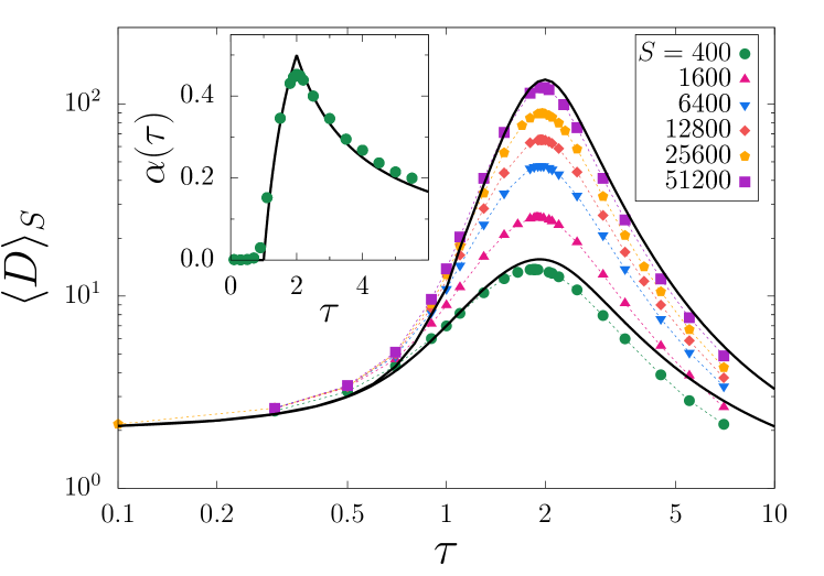
Figure 2: Average diversity, $\langle D\rangle_{S}$, obtained through numerical simulations for various sizes $S$ (see key), dashed lines are guides to the eye. Entities are extracted from the bare distribution Eq. (6) and the statistics is restricted over configurations respecting the global constraint. Results are averaged over $10^{4}$-$10^{6}$ configurations. Solid lines (shown only for the extreme sizes), are the analytical solutions given by Eq. (10). Inset: The exponent $\alpha(\tau)$, defined below Eq. (11), as a function of $\tau$. Solid line is the analytical result, dots are fits from the simulation data.

For large $S$, the leading contribution to Eq. (10) is

$$\langle D\rangle_{S}\simeq\begin{cases}\displaystyle(2-\tau)/(1-\tau)&;\,\text{for}\quad\tau<1\\ \ln S&;\,\text{for}\quad\tau=1\\ \displaystyle\frac{\tau(2-\tau)^{1/\tau}}{\tau-1}S^{1-1/\tau}&;\,\text{for}\quad 1<\tau<2\\ \displaystyle 2\left(S/\ln S\right)^{1/2}&;\,\text{for}\quad\tau=2\\ \displaystyle\frac{\tau}{\tau-1}\left[\frac{S}{\gamma+(\tau-2)^{-1}}\right]^{1/\tau}&;\,\text{for}\quad\tau>2\ .\end{cases}$$ (11)

One has $\langle D\rangle_{S}\sim S^{\alpha(\tau)}$ with $\alpha(\tau)=0$ for $\tau<1$, $\alpha(\tau)=1-1/\tau$ for $1<\tau<2$ and $\alpha(\tau)=1/\tau$ for $\tau>2$, see inset of Fig 2. In conclusion, for large $S$, $\langle D\rangle_{S}$ presents a pronounced peak at $\tau=2$. This behavior is due to the competition between the abundance of entities $\langle N\rangle_{S}$, favored by large $\tau$, and the diversity of their sizes which instead is enhanced by small $\tau$, as shown in Fig. 1. We remark that the upper bound obtained by considering the deterministic partition $S\simeq 1+2+\ldots+D$ with $D\sim S^{1/2}$ overpowers the $\tau=2$ case only by a logarithmic factor.

Let us mention that, although we explicitly solved the model for power law distributions, which yield maximum diversity, our calculations can be straightforwardly generalized to different $p(s)$. For instance, in the case of algebraic distributions with a lower cut-off, a case often representative of real situations De Marzo et al. (2021), one recovers similar results provided that the cut-off is independent of $S$ (see the SM Sup ).

We also stress that, as shown in the SM Sup , among the possible measures of diversity usually considered in the literature, $D$ is the only one to be maximized in connection with Zipf’s law.

We notice also that the model considered here is related to the random allocation model Godrèche (2019) where the resource $S$ is distributed among an assigned number $N$ of components. The diversity properties of such model, however, are very different and, in particular, the special role played by $\tau=2$ is missing. This is briefly discussed in the SM Sup .

Diversity, Zipf’s and Heaps’ laws.— Since the diversity is determined once an empirical distribution of sizes is given, we can use $\langle D\rangle_{S}$ given in Eq. (11) to estimate the diversity index $D$ of power law distributed empirical data, regardless of the mechanism whereby they are produced. If this assumption holds, on the basis of our analytical arguments, one can conclude that if a system displays Zipf’s law ($\tau\simeq 2$) it is at the edge of maximal diversity and vice versa.

As a first example we consider quantitative linguistics, the field in which Zipf’s law has been originally observed in almost every human language Condon (1928); Piantadosi (2014); Gerlach and Altmann (2014); Moreno-Sánchez et al. (2016). The regime of validity of the law in this context Font-Clos et al. (2013), its deviations Ferrer-i-Cancho (2005) and the underlying mechanism(s) are still a matter of dispute. Nonetheless, large scale studies have been performed in order to validate that. For example, Moreno-Sánchez et al. Moreno-Sánchez et al. (2016) considered a very large set of English books (more than 30000) from the Gutenberg Project database. They checked how well some simple, one-parameter forms of the Zipf’s law describe these data on the whole interval of frequencies, finding very good agreement with a distribution of exponents centered on $\tau\simeq 2$.

We use the filtered data of Ref. Moreno-Sánchez et al. (2016) and, for each book, measure the diversity index $D$. The total number of words a book contains is its total size $S$, the number of distinct words is the number of entities, $N$, and the size $s$ of each entity is its absolute frequency, i.e. how many times that word appears. The diversity $D$ is therefore the number of different frequencies a given text displays. The result of this analysis is shown in Fig. 3 along with Eq. (11) for $\tau=2$. Notice that there are no free parameters in the plot. The agreement between our theoretical prediction and the experimental points is consistent with the results reported in Ref. Moreno-Sánchez et al. (2016) showing that a great deal of the books have $\tau$ close to 2.

As a second example, we consider how the total population $S$ of a country is distributed among its cities. We use data for European countries from the GeoNames database Geo , for which Simini and James Simini and James (2019) showed that the size $s$ of cities closely follows a Zipf’s distribution ($\tau\simeq 2.02$). The diversity index $D$ is shown in Fig. 3 (bottom panel). Since cities cannot be smaller than a certain lower cutoff $s_{L}$, the analytical prediction to compare with is Eq. (29) of the SM, see SM Sup , (solid line). Despite the noisy character of the data, there is a very good agreement between the data and our theory.

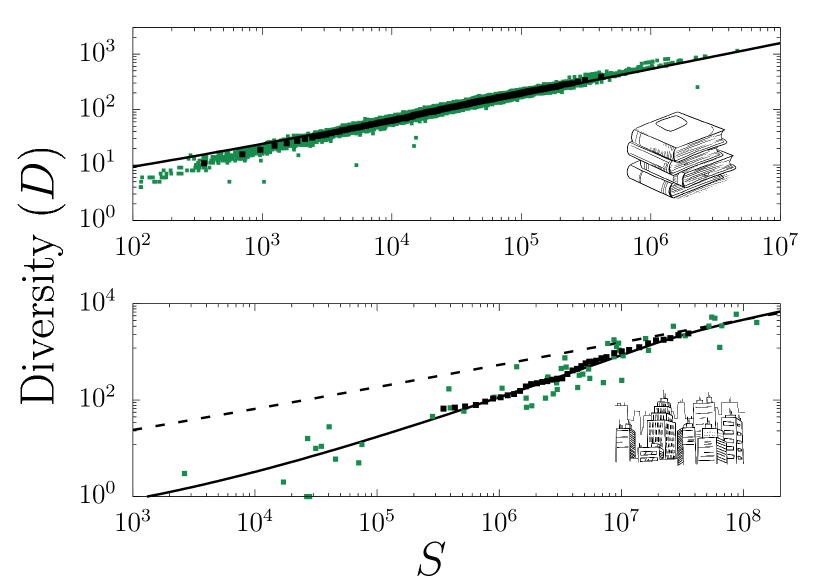
Figure 3: (Top panel) Diversity index $D$ evaluated from the data of Ref. Moreno-Sánchez et al. (2016). Each green point is one of the more than 30000 English books in the Project Gutenberg database (accessed July 2014), while the black squares are a running average over 20 points. The solid line is the result $\langle D\rangle_{S}=2(S/\ln S)^{1/2}$, from Eq. (11) for $\tau=2$, which corresponds to maximal diversity. (Bottom panel) Diversity index using data from the GeoNames database Geo for cities. Each green point is an European country and the black squares are the corresponding running average. The solid line is Eq. (29) of the SM Sup where the presence of a lower cutoff $s_{L}$ is taken into account. $s_{L}$ is estimated from the average of the smallest city in each country ($s_{L}\simeq 1313$), see SM Sup . The dashed line is the behavior $\langle D\rangle_{S}=2(S/\ln S)^{1/2}$, which is approached only asymptotically.

The content of Eq. (8) is Heaps’ law, which gives an estimate of the number of components of a system of total size $S$ given that the empirical size distribution follows a power law with exponent $\tau$. Our expression of the law for $\tau>1$ is in accordance with Ref. Lü et al. (2010) and complements the result with the cases with $\tau\leq 1$ and with the appropriate prefactors. Heap’s law is expected to hold for systems which are robust in the statistics of their component ($p_{S}(s)$ in our notation) at varying $S$ Lü et al. (2010); De Marzo et al. (2021). This is captured in our approach, where Eq. (8) is only arrived at using distributions which have the same form for any $S$ (the same applies to Eq. (11)).

In our approach, Heap’s law (8) and the diversity law (11) imply each other, encoding dependencies on the system size on equal footings. However, notably, the latter naturally selects the exponent $\tau=2$ as a special one. Moreover, our analysis of the Gutenberg dataset shows that the diversity law is obeyed up to the largest sizes considered ($S\simeq 10^{7}$), whereas it is known Lü et al. (2013) that strong deviations from Heaps’ law are caused by the finiteness of the vocabulary. Therefore, at least in the context of language, the diversity law appears more robust and this suggests that its use could be more suited to interpret the size dependence of empirical data.

Discussion.— The partition of a finite resource $S$ among constituents informs numerous systems in diverse fields of science and humanities. In this Letter, by solving a paradigmatic statistical model, we have shown that a maximally diverse partition is accompanied by Zipf’s law. Such co-occurrence is a general property of the empirical distribution, holding irrespectively of the specific mechanisms at work in generating Zipfian behavior in given systems.

Diversity and information are fundamental concepts for the description of complex statistical systems whose formalization led to the definition of a coherent set of quantitative measures, Boltzmann-Shannon entropy above all. Our results show that in the case of system obeying Zipf’s law an important role is played by one of such measures, the index $D$. When framed in terms of extremization of appropriate cost functions, problems are endowed with a complementary description and can be approached with new strategies. Our study suggests that, in some instances where Zipf’s law is empirically observed, promoting diversity to the role of a driving force could provide further theoretical insights towards a deeper and more general comprehension.

O.M. is indebted with I. A. Hatton, M. Smerlak and A. Zadorin for numerous and insightful discussions and acknowledges the Alexander von Humboldt Foundation in the framework of the Sofja Kovalevskaja Award endowed by the German Federal Ministry of Education and Research for providing funding for this work. A.A.L. and J.J.A. thank Salerno University for hospitality. A.A.L acknowledges the Brazilian funding agency CAPES in the framework of the Capes-PrInt program (grant 88887.466912/2019-00). J.J.A. thanks the Brazilian funding agency CNPq (grant 308927/2017-6). The authors thank S. Bora for the drawings in Fig. 3.

References

- Jost (2006) L. Jost, Oikos 113, 363 (2006).
- Tuomisto (2010) H. Tuomisto, Oecologia 164, 853 (2010).
- Ives and Carpenter (2007) A. R. Ives and S. R. Carpenter, Science 317, 58 (2007).
- Elton (1958) C. S. Elton, The ecology of invasions by animals and plants (Methuen & Co. Ltd., London, UK, 1958).
- Tilman et al. (2006) D. Tilman, P. B. Reich, and J. M. Knops, Nature 441, 629 (2006).
- Arese Lucini et al. (2020) F. Arese Lucini, F. Morone, M. S. Tomassone, and H. A. Makse, PLOS ONE 15, 1 (2020).
- Tacchella et al. (2012) A. Tacchella, M. Cristelli, G. Caldarelli, A. Gabrielli, and L. Pietronero, Sci. Rep. 2, 723 (2012).
- Rényi et al. (1961) A. Rényi et al., in Proceedings of the Fourth Berkeley Symposium on Mathematical Statistics and Probability, Volume 1: Contributions to the Theory of Statistics (The Regents of the University of California, 1961).
- Tsallis (1988) C. Tsallis, J. Stat. Phys. 52, 479 (1988).
- (10) See Supplemental Material for an account of Rényi entropies, their connection with diversity indices and arguments for studying specifically the diversity index considered in this paper based on numerical simulations, an explicit expression for the probability distribution of the diversity , an exact computation of the dressed probability distribution and , motivations for the approximation , the case of power law bare distributions with a lower cut-off and details of the analysis of population datasets and an account of the behaviour of diversity in the random allocation model. Ref. Corberi (2017) is included.
- Gabaix (1999) X. Gabaix, The Quarterly Journal of Economics 114, 739 (1999).
- Piantadosi (2014) S. T. Piantadosi, Psychon Bull Rev. 21, 1112 (2014).
- Furusawa and Kaneko (2003) C. Furusawa and K. Kaneko, Phys. Rev. Lett. 90, 088102 (2003).
- Zipf (1949) G. K. Zipf, Human Behaviour and the Principle of Least Effort: An Introduction to Human Ecology (Addison-Wesley, Cambridge, MA, 1949).
- Newman (2005) M. E. J. Newman, Contemp. Phys. 46, 323 (2005).
- Clauset et al. (2009) A. Clauset, C. R. Shalizi, and M. E. Newman, SIAM Review 51, 661 (2009).
- Cristelli et al. (2012) M. Cristelli, M. Batty, and L. Pietronero, Sci. Rep. 2, 812 (2012).
- Axtell (2001) R. L. Axtell, Science 293, 1818 (2001).
- Willis and Yule (1922) J. C. Willis and G. U. Yule, Nature 109, 177 (1922).
- Oddershede et al. (1993) L. Oddershede, P. Dimon, and J. Bohr, Phys. Rev. Lett. 71, 3107 (1993).
- Corral et al. (2020) A. Corral, I. Serra, and R. Ferrer-i-Cancho, Phys. Rev. E 102, 052113 (2020).
- Simon (1955) H. A. Simon, Biometrika 42, 425 (1955).
- Levy and Solomon (1996) M. Levy and S. Solomon, Int. J. Mod. Phys. C 7, 595 (1996).
- Marsili and Zhang (1998) M. Marsili and Y.-C. Zhang, Phys. Rev. Lett. 80, 2741 (1998).
- Ferrer-i-Cancho and Solé (2003) R. Ferrer-i-Cancho and R. V. Solé, Proceedings of the National Academy of Sciences 100, 788 (2003).
- Tria et al. (2014) F. Tria, V. Loreto, V. D. P. Servedio, and S. H. Strogatz, Sci. Rep. 4, 5890 (2014).
- Corominas-Murtra et al. (2015) B. Corominas-Murtra, R. Hanel, and S. Thurner, Proceedings of the National Academy of Sciences 112, 5348 (2015).
- Mazzolini et al. (2018) A. Mazzolini, M. Gherardi, M. Caselle, M. C. Lagomarsino, and M. Osella, Phys. Rev. X 8, 021023 (2018).
- Mora and Bialek (2011) T. Mora and W. Bialek, J. Stat. Phys. 144, 268 (2011).
- Marsili et al. (2013) M. Marsili, I. Mastromatteo, and Y. Roudi, J. Stat. Mech.: Theory and Experiment 2013, P09003 (2013).
- Schwab et al. (2014) D. J. Schwab, I. Nemenman, and P. Mehta, Phys. Rev. Lett. 113, 068102 (2014).
- Cubero et al. (2019) R. J. Cubero, J. Jo, M. Marsili, Y. Roudi, and J. Song, J. Stat. Mech.: Theory and Experiment 2019, 063402 (2019).
- (33) Project Gutenberg, www.gutenberg.org.
- (34) GeoNames, www.geonames.org.
- Heaps (1978) H. S. Heaps, Information Retrieval: Computational and Theoretical Aspects (Academic Press, Inc., Orlando, FL, 1978).
- Lü et al. (2010) L. Lü, Z.-K. Zhang, and T. Zhou, PLOS ONE 5, e14139 (2010).
- de Azevedo-Lopes et al. (2020) A. de Azevedo-Lopes, A. R. de la Rocha, P. M. C. de Oliveira, and J. J. Arenzon, Phys. Rev. E 101, 012108 (2020).
- De Marzo et al. (2021) G. De Marzo, A. Gabrielli, A. Zaccaria, and L. Pietronero, Phys. Rev. Research 3, 013084 (2021).
- Godrèche (2019) C. Godrèche, Journal of Statistical Mechanics: Theory and Experiment 2019, 063207 (2019).
- Condon (1928) E. U. Condon, Science 67, 300 (1928).
- Gerlach and Altmann (2014) M. Gerlach and E. G. Altmann, New J. Phys. 16, 113010 (2014).
- Moreno-Sánchez et al. (2016) I. Moreno-Sánchez, F. Font-Clos, and A. Corral, PLOS ONE 11, 1 (2016).
- Font-Clos et al. (2013) F. Font-Clos, G. Boleda, and A. Corral, New J. Phys. 15, 093033 (2013).
- Ferrer-i-Cancho (2005) R. Ferrer-i-Cancho, Eur. Phys. J. B 44, 249 (2005).
- Simini and James (2019) F. Simini and C. James, EPJ Data Science 8, 24 (2019).
- Lü et al. (2013) L. Lü, Z.-K. Zhang, and T. Zhou, Sci. Rep. 3, 1082 (2013).
- Corberi (2017) F. Corberi, Phys. Rev. E 95, 032136 (2017).