Cascade of singularities in the spin dynamics of a perturbed quantum critical Ising chain

Abstract

When the quantum critical transverse-field Ising chain is perturbed by a longitudinal field, a quantum integrable model emerges in the scaling limit with massive excitations described by the exceptional $E_{8}$ Lie algebra. Using the corresponding analytical form factors of the quantum $E_{8}$ integrable model, we systematically study the spin dynamic structure factor of the perturbed quantum critical Ising chain, where particle channels with total energy up to 5$m_{1}$ ($m_{1}$ being the mass of the lightest $E_{8}$ particle) are exhausted. In addition to the significant single-particle contributions to the dynamic spectrum, each two-particle channel with different masses is found to exhibit an edge singularity at the threshold of the total mass and decays with an inverse square root of energy, which is attributed to the singularity of the two-particle density of states at the threshold. The singularity is absent for particles with equal masses due to a cancellation mechanism involving the structure of the form factors. As a consequence, the dynamic structure factor displays a cascade of bumping peaks in the continuum region with clear singular features which can serve as a solid guidance for the material realization of the quantum $E_{8}$ model.

I introduction

Due to collective quantum fluctuations, exotic states of matter can emerge near a quantum critical point (QCP) in quantum many-body systems [Sachdev, 2011; Belavin et al., 1984; Zamolodchikov and Zamolodchikov, 1979; Belavin et al., 2004; Delfino and Mussardo, 1994; Berg et al., 1979], which have been attracting intensive research [v. Löhneysen, 2010; Si et al., 2001; Coleman and Schofield, 2005; Schuberth et al., 2016; Wu et al., 2014; Wang et al., 2018; Wu et al., 2018; Wang et al., 2019; Cui et al., 2019; Fan et al., 2020]. One such paradigmatic system is the transverse field Ising chain (TFIC) in the presence of a longitudinal field. At the QCP of the TFIC, conformal invariance emerges in the scaling limit, corresponding to a central charge 1/2 conformal field theory (CFT). Turning on a small longitudinal field at the QCP gives a perturbation to the conformal field theory, resulting in a massive relativistic field theory model with an emergence of eight stable particles of masses $m_{i},i=1,\cdots,8$ (Fig. 1) [Zamolodchikov, 1989]. The mass ratios of the eight particles and their scatterings and form factors are beautifully organized by the $E_{8}$ exceptional Lie algebra, dubbed as the quantum $E_{8}$ integrable model  [Dorey, 1997; Zamolodchikov, 1989].

A material realization has been long sought since the discovery of the quantum $E_{8}$ integrable model. One decade ago, inelastic neutron scattering measurements in quasi-one-dimensional (1D) ferromagnetic CoNb₂O₆ provided preliminary evidence for the lowest two states of the quantum $E_{8}$ spectrum corresponding to the lightest two particles with masses $m_{1}$ and $m_{2}$ [Coldea et al., 2010], which further motivated material-based studies of this exotic system [Kjäll et al., 2011]. Recently, a combination of theoretical and experimental efforts led to a full realization of the quantum $E_{8}$ spectrum in the material of BaCo₂V₂O₈ (BCVO) [Zhang et al., 2020; Zou et al., 2020]. In Refs. [Zhang et al., 2020; Zou et al., 2020], besides a direct physical instruction to concretely guide the experimental realization of the quantum $E_{8}$ spectrum in BCVO, we also provided a summary of an analytical form factor framework to determine the corresponding dynamical structure factor (DSF). The analytical DSF data in Refs. [Zhang et al., 2020; Zou et al., 2020] have been broadened in accord with realistic experimental energy resolution. The excellent agreement implies the first experimental realization of the quantum $E_{8}$ integrable model in a real material. Motivated by this exciting progress, in this paper we give a complete account of the details of the analytic calculations, greatly expanding the discussion presented in the recent experimental-theoretical work [Zhang et al., 2020; Zou et al., 2020] on the material realization of the quantum $E_{8}$ model in BaCo₂V₂O₈.

When unfolding details of the analytical framework, we uncover rich features not revealed in Refs. [Zhang et al., 2020; Zou et al., 2020], such as the singular structure of the DSF spectrum smeared in the broadened analytical DSF data [Zhang et al., 2020; Zou et al., 2020]. We find that besides the well-known singularities from the single-$E_{8}$-particle channels, the two-particle channels with different masses lead to a cascade of edge singularities in the dynamic spectrum, where the threshold for each edge singularity is the total mass of the two particles. When energy  is beyond the edge-singularity threshold, the two-particle spectrum decays in a power of an inverse square root. This singularity can be traced to the divergence of the two-particle density of states (DOS) at the threshold which, however, is accidentally canceled for two-particle channels with equal masses due to the special analytical structure of the form factors. We further demonstrate the smoothness and quick decrease of the contributions of three and more particle channels to the DSF. Due to the rapidly decreasing spectral weight and exponentially increasing CPU cost of carrying out the multi-fold integration with increasing particle number, we choose the energy cutoff at 5$m_{1}$ and focus on zero total momentum in all DSF calculations. The DSF for non-zero momentum as well as the corresponding dispersion are deferred to future study.

The rest of the paper is organized as follows. Sec. II elaborates the necessary ingredients of our calculations. Sec. III provides analytical calculations in detail. Then we discuss our results with experimental realization and draw conclusion in Sec. IV. The details of the analytic calculations can be found in the Appendices, including the complete and correct set of recursive equations for systematically obtaining the form factors of the quantum $E_{8}$ model.

II The model

We consider the transverse-field Ising chain (TFIC) at its QCP $g=g_{c}=1$ perturbed by a longitudinal field $h_{z}$,

$$H_{\text{pert}}=-J(\sum_{i}\sigma_{i}^{z}\sigma_{i+1}^{z}+\sum_{i}\sigma_{i}^{x}+h_{z}\sum_{i}\sigma_{i}^{z}),$$ (1)

where $J>0$, and $\sigma_{i}^{\alpha}$ at site $i$ are the Pauli matrices related to the spin operators $S_{i}^{\alpha}=\sigma_{i}^{\alpha}/2,$ $(\alpha=x,y,z)$ with the Planck constant set to $\hbar=1$. In the scaling limit, the QCP is described by the conformal field theory of central charge $c=1/2$ corresponding to free massless fermions. The Hamiltonian (1) gives rise to a field theory obtained by perturbing the CFT by one of its relevant primary operator [Dorey, 1997; Wu et al., 2014; McCoy and Wu, 1978],

$$H_{E_{8}}=H_{c=1/2}-h\int dx\,\sigma(x)\,,$$ (2)

where the operator $\sigma(x)$ and the field $h$ are the rescaled field theory versions of the lattice magnetization operator $\sigma_{i}^{z}$ and longitudinal magnetic field $h_{z},$ respectively (for the precise relations c.f. Appendix A).

As shown by Zamolodchikov [Zamolodchikov, 1989], this perturbation opens a gap and leads to an integrable quantum field theory, the so-called $E_{8}$ model. The hallmark of this model is the presence of eight stable particle excitations [Delfino and Mussardo, 1995] with the mas of the lightest particle is $m_{1}\sim|h|^{8/15}$ and all the other masses can also be expressed in terms of $m_{1}$ exactly, as shown in Fig. 1.

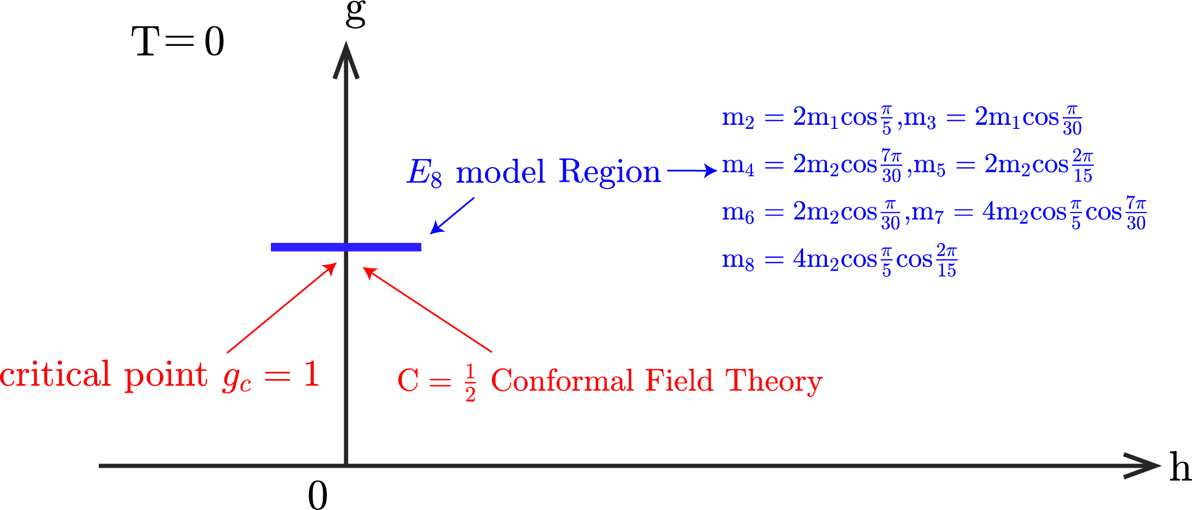
Figure 1: The blue solid line illustrates the region $E_{8}$ physics emerges, where parameters $h$ and $g$ for horizontal and vertical axes are from the Hamiltonian Eq. (1). The masses of particles are displayed in terms of the lightest two masses $m_{1}$ and $m_{2}.$

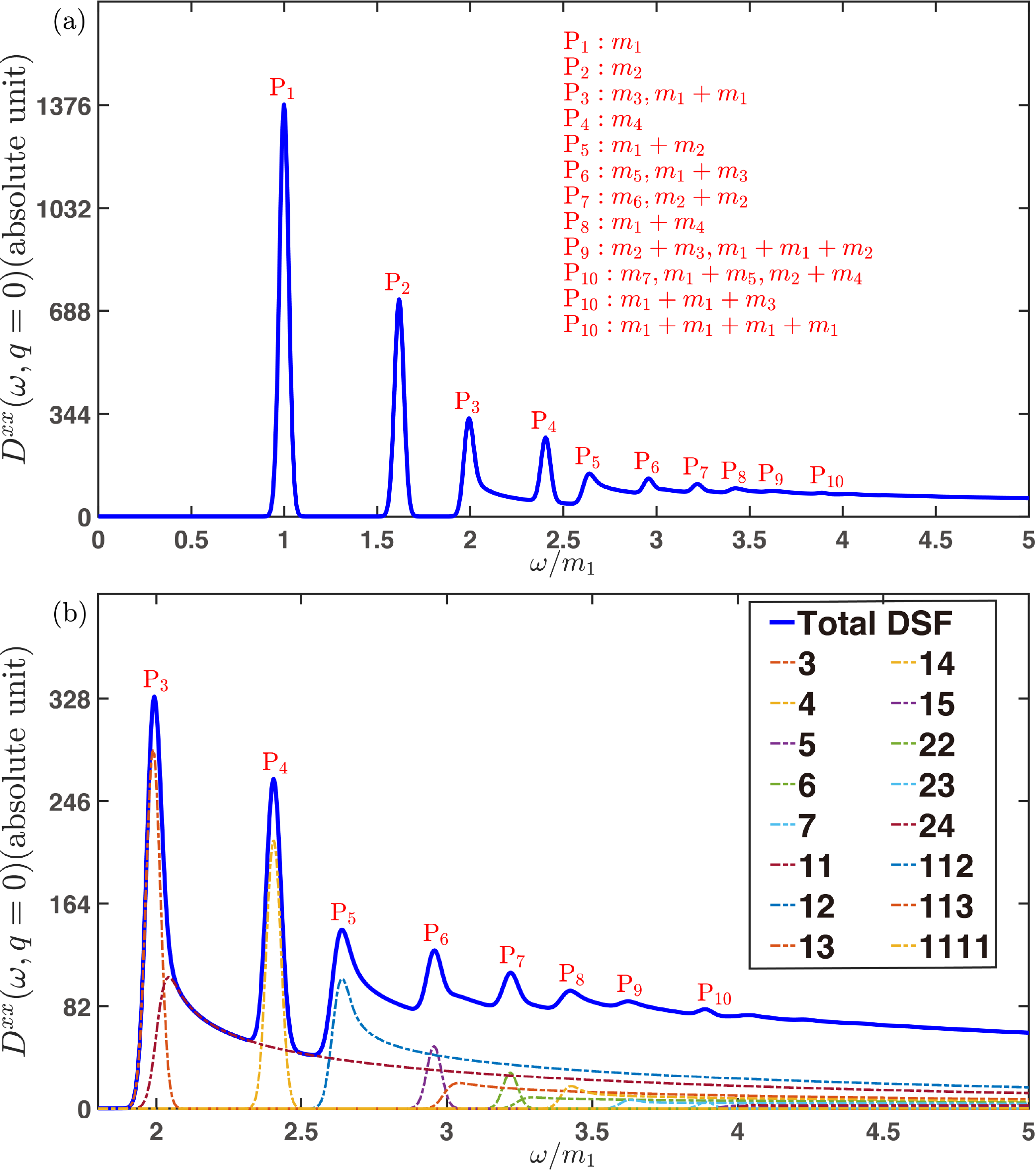
Figure 2: The total $D^{xx}(\omega,q=0)$ intensity as a function of $\omega$ with 0.05$m_{1}$ broadening. (a) Several peaks associated with single or multi-particle excitations are labelled by $P_{i}$, where $i=1$ to 10 as $\omega$ increases. (b) The details of spectrum with excitation energy larger than $2m_{1}$. Each dashed curve is the DSF from the corresponding channel. The numbers in the legend are abbreviated labels for $E_{8}$ particles. For example, “11” stands for $m_{1}+m_{1}$ channel.

The energy and momentum eigenstates of the Hamiltonian can be written as asymptotic states $|A(\theta_{1}),...,A(\theta_{n})\rangle_{a_{1},...,a_{n}}$ with the orthogonality and normalization relations

$${}_{a_{i}}\langle A(\theta_{i})|A(\theta_{j})\rangle_{a_{j}}=2\pi\delta_{a_{i}a_{j}}\delta(\theta_{i}-\theta_{j}),$$ (3)

where $|A(\theta_{i})\rangle_{a_{i}}$ ($a_{i}=1,\cdots,8$) labels a state of an $E_{8}$ particle with mass $m_{a_{i}}$ and rapidity $\theta_{i}$. The energy and momentum eigenvalues written in terms of the relativistic rapidity parameter $\theta$ are $E=\sum_{i=1}^{n}m_{a_{i}}\cosh(\theta_{i})$ and $P=\sum_{i=1}^{n}m_{a_{i}}\sinh(\theta_{i})$, respectively.

In the following, we consider the two point correlation function of the operators $\Phi=\sigma^{x,y,z}$,

$$\langle\Phi(x,t)\Phi(0,0)\rangle=\langle 0|e^{-iPx}e^{iHt}\Phi(0,0)e^{-iHt}e^{iPx}\Phi(0,0)|0\rangle$$ (4)

where $|0\rangle$ stands for the ground state (vacuum) of the $E_{8}$ Hamiltonian. By inserting a complete basis of the $E_{8}$ eigenstates into the correlation function, the dynamic structure factor (DSF) with zero momentum transfer expressed in the Lehmann representation follows as

$$D^{\Phi\Phi}(\omega,q=0)\\ =\sum_{n=0}^{\infty}\sum_{\{a_{i}\}}(\prod_{a_{i}}\dfrac{1}{N_{a_{i}}!})\dfrac{1}{(2\pi)^{n-2}}\int_{-\infty}^{\infty}d\theta_{1}...d\theta_{n}\\ |\langle 0|\Phi|A(\theta_{1}),...,A(\theta_{n})\rangle_{a_{1},...,a_{n}}|^{2}\delta(\omega-\sum_{i=1}^{n}E_{i})\delta(\sum_{i=1}^{n}p_{i}).$$ (5)

As Eq. (5) shows, the dynamic properties of the system are determined by the combined effects from the on-shell particles with total energy and momentum conservation. By choosing different number of particles in the complete basis, the contributions of the DSF can be divided into different channels: single-, two-, three-particle channels and so on. Each channel’s DSF contribution exhibits special features as shall be discussed in the following sections. To calculate Eq. (5), the form factors

$$F_{a_{1},...,a_{n}}^{\Phi}(\theta_{1},...,\theta_{n})=\langle 0|\Phi|A(\theta_{1}),...,A(\theta_{n})\rangle_{a_{1},..,a_{n}},$$ (6)

are needed, which can be derived following the form factor bootstrap approach [Delfino and Mussardo, 1995; Delfino and Simonetti, 1996; Hódsági et al., 2019; Schuricht and Essler, 2012; Bertini et al., 2014; Cortés Cubero and Schuricht, 2017]. The detailed form of the recursive equations and a discussion of the method of solving them are presented in Appendix C.

For practical calculations, the infinite form factor series must be truncated. In this work, we systematically calculate the form factor contributions up to the energy cutoff at $5m_{1}$.

III The spin dynamic structure factor of the quantum $E_{8}$ integrable model

We now proceed to calculate the DSF $D^{\Phi\Phi}(\omega,q=0)$ with $\Phi=\sigma^{i}$ and $i=x,y,z$ (abbreviated as $D^{ii}$) for the $E_{8}$ model. There are two relevant operators, $\sigma(x)$ (magnetization density) and $\epsilon(x)$ (energy density) in the $E_{8}$ model, corresponding to $\sigma_{i}^{z}$ and $\sigma_{i}^{x}$ in the lattice model [Delfino and Mussardo, 1995], respectively (see also Appendix A). As a result, within the framework of quantum $E_{8}$ integrable model, one is only able to determine $D^{xx}$ and $D^{zz}$. $D^{yy}$ can be determined through an exact relation $D^{yy}(\omega)=\omega^{2}D^{zz}(\omega)/(4J^{2})$ [Wu et al., 2014]. $D^{xx}(\omega,q=0)$ is shown in Fig. 2, and the results for $D^{yy}(\omega,q=0)$ and $D^{zz}(\omega,q=0)$ can be found in the Appendix G. [SM, ].

For illustration, in Fig. 2 we broaden the DSF with an energy resolution of $0.05m_{1}$. When the transferred energy is larger than $2m_{1}$, multi-particle excitations appear. Remarkably, the high energy excitations retain visibility in the DSF continuum region (Fig. 2) up to $m_{7}$. In particular, the various two-particle spectrum contributions leave significant “resonant” features with bumpy peaks in the continuum region of the spectrum, whose origin will be discussed in detail in Sec. III.2. The clear observation of this theoretically expected series of two-particle peaks at the corresponding transferred energy in the material of BCVO [Zhang et al., 2020; Zou et al., 2020] provides a smoking gun signature for the material realization of the $E_{8}$ model.

In the following, to analyze contributions from the single and multi-particle excitations in detail, we specify the contributions of the different channels according to the number of particles and exhaust all possible cases with energy less than $5m_{1}>m_{8}$.

III.1 Single-particle channels

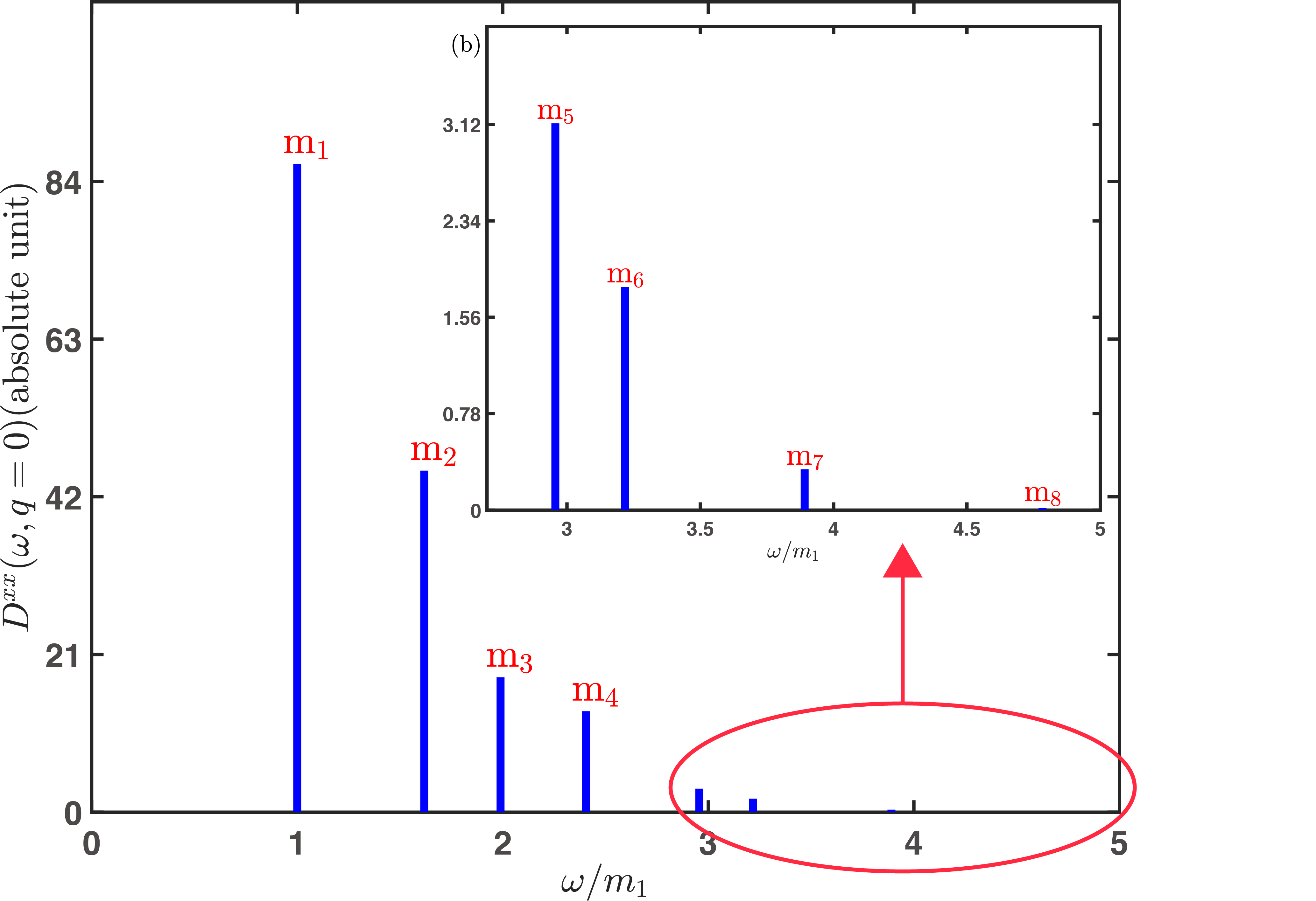
Figure 3: $D^{xx}_{1}(\omega,q=0)$ contribution from the single particle channels are delta functions with different spectral weights for different $E_{8}$ particle species. The inset exhibits the spectral weights from $m_{5}$ through $m_{8}$.

The single-particle contributions to DSF are given by

$$D^{\Phi\Phi}_{1}(\omega,q=0)=\sum_{i=1}^{8}2\pi\dfrac{|F^{\Phi}_{a_{i}}|^{2}}{m_{a_{i}}}\delta(\omega-m_{a_{i}}),$$ (7)

where the form factor $F_{a_{i}}^{\Phi}$ is the single particle form factor for the $E_{8}$ particle $a_{i}$ [Delfino and Simonetti, 1996], and $2\pi|F^{\Phi}_{a_{i}}|^{2}/{m_{a_{i}}}$ gives the corresponding single-particle spectral weight. In Fig. 3 we show the spectral weight of $D^{xx}_{1}$ for each $E_{8}$ particle.

III.2 Two-particle channels

From Eq. (5), we get following two-particle contributions to the DSF,

$$D^{\Phi\Phi}_{2}(\omega,q=0)=\sum_{i\leq j}(\dfrac{1}{2})^{\delta_{a_{i}a_{j}}}\dfrac{|F^{\Phi}_{a_{i}a_{j}}(\theta_{1}-\theta_{2})|^{2}}{m_{a_{i}}m_{a_{j}}|\sinh(\theta_{1}-\theta_{2})|},$$ (8)

where

$$\theta_{1}-\theta_{2}=\text{arccosh}\left(\dfrac{\omega^{2}-m_{a_{i}}^{2}-m_{a_{j}}^{2}}{2m_{a_{i}}m_{a_{j}}}\right)\,,$$ (9)

with the lower bound of energy as $\omega_{min}=m_{a_{i}}+m_{a_{j}}$, the spectrum threshold for a specific two-particle channel with masses $m_{a_{i}}$ and $m_{a_{j}}$.

Fig. 4 shows the analytical two-particle DSF results of $D^{xx}_{2}$ by considering all possible combinations with $\omega<5m_{1}$. Edge singularities are exhibited for two-particle channels with different masses. In Eq. (8), the Jacobian term $1/|\sinh(\theta_{1}-\theta_{2})|,$ which is just the two-particle density of states, contributes a singular behavior at $\theta_{1}=\theta_{2}$, corresponding to $\omega=\omega_{0}$ ($\omega_{0}=m_{a_{i}}+m_{a_{j}}$). A simple analysis gives $D_{2}^{xx}\sim 1/\sqrt{\omega-\omega_{0}}$ at $\omega\gtrsim\omega_{0}$  [SM, ]. Apparently, this singular behavior also appears in $D^{yy}$ and $D^{zz}$. This scaling behavior is further illustrated in Fig. 4(b) by the logarithmic fitting of $D^{xx}$ at $m_{1}m_{2}$ channel with fitting $(\omega-\omega_{0})^{\alpha}$, $\alpha=-0.5043$. The edge singularity disappears for two particles with the same mass, which is due to the explicit form of equal-mass-two-particle form factor where a $|\sinh^{2}(\theta_{1}-\theta_{2})/2|$ term appears and cancels the $\sinh(\theta_{1}-\theta_{2})$ in the denominator of Eq. (8) [SM, ].

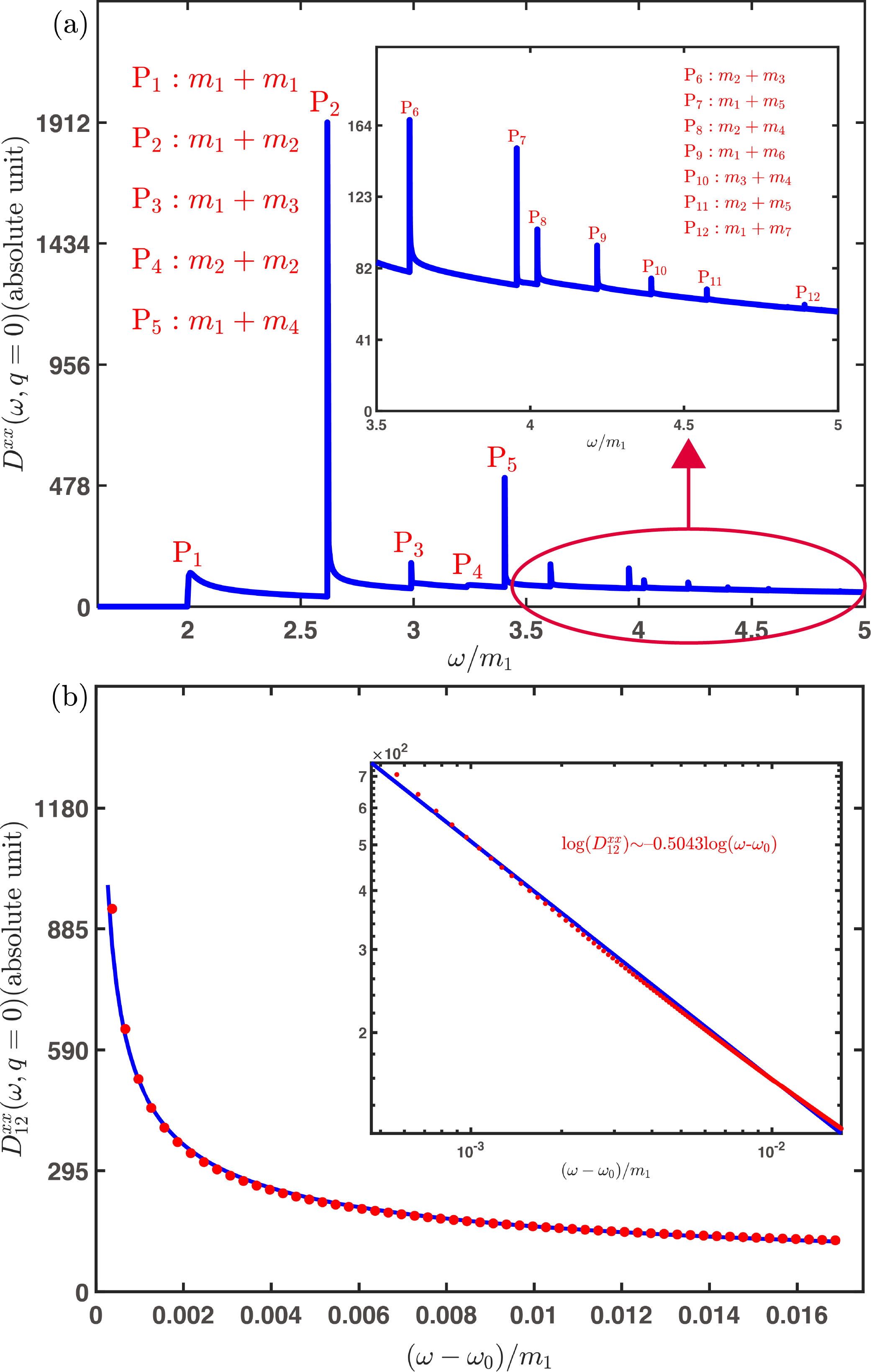
Figure 4: The two-particle DSF. (a) $D^{xx}_{2}(\omega,q=0)$ contributed from all two-particle channels. The $\omega>3.5m_{1}$ region is highlighted in the inset. (b) The singularity near the peak arise at $\omega_{0}=m_{1}+m_{2}$ has an inverse square root $\sim(\omega-\omega_{0})^{-1/2}$ behavior, confirmed by the logarithmic fit for the $m_{1}+m_{2}$ channel shown in the inset.

III.3 Three and four-particle channels

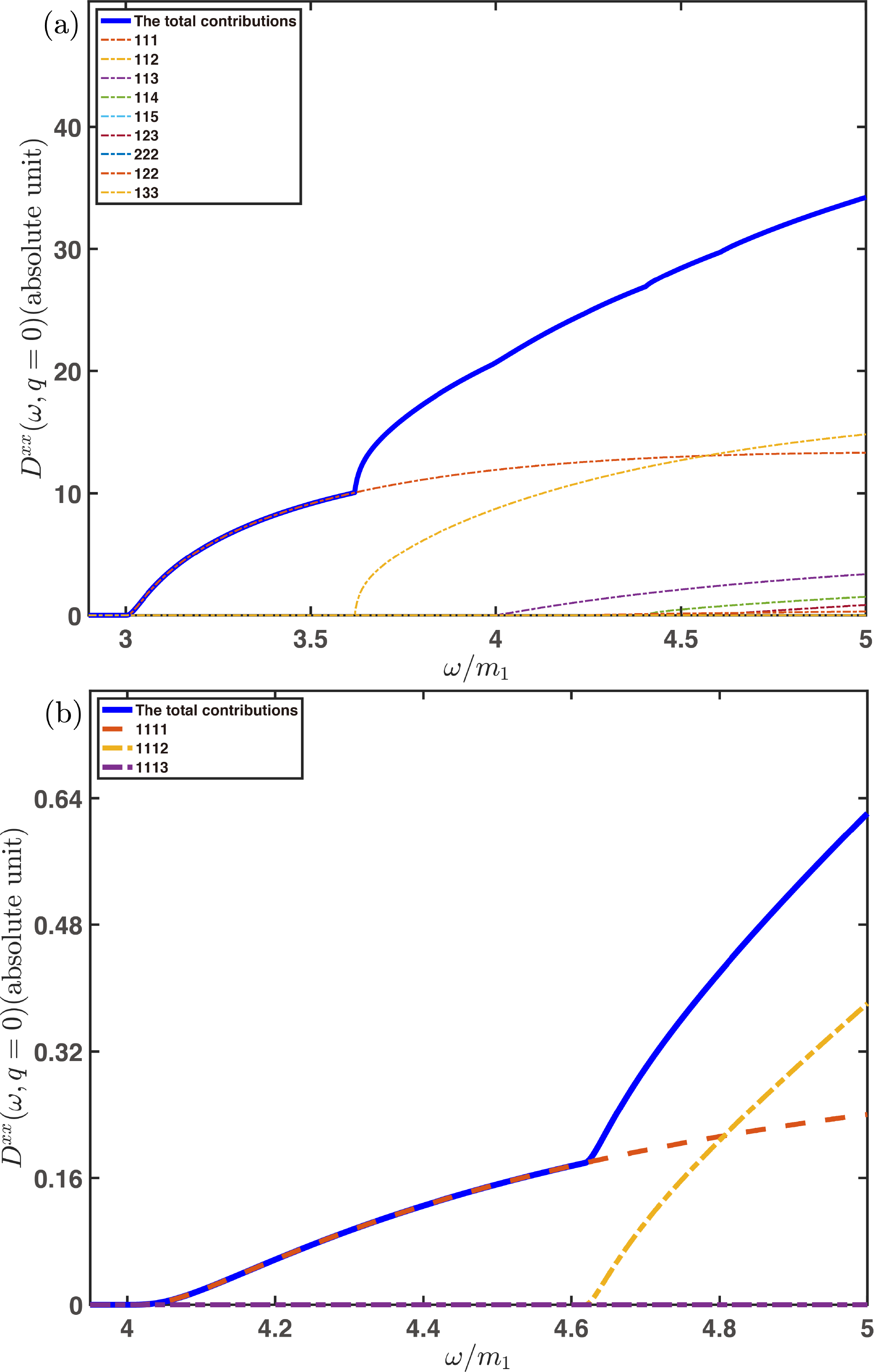
Figure 5: $D^{xx}(\omega,q=0)$ from three-particle channels (a) and four-particle channels (b) for $\omega<5m_{1}$.

In this section we further determine the contributions of multi-particle channels beyond two particles. From Eq. (5), we have DSF contributions

$$D^{\Phi\Phi}_{3}(\omega,q=0) =\sum_{i\leq j\leq k}(\prod_{a_{i,j,k}}\dfrac{1}{N_{a}!})\dfrac{1}{(2\pi)}$$ (10)

$$\times\int_{-\infty}^{\infty}d\theta_{3}\dfrac{|F^{\Phi}_{a_{i}a_{j}a_{k}}(\theta_{1},\theta_{2},\theta_{3})|^{2}}{m_{a_{i}}m_{a_{j}}|\sinh(\theta_{1}-\theta_{2})|}$$

for the three-particle channels, and

$$D^{\Phi\Phi}_{4}(\omega,q=0)=\sum_{i\leq j\leq m\leq n}(\prod_{a}\dfrac{1}{N_{a}!})\dfrac{1}{(2\pi)^{2}}$$ (11)

$$\times\int_{-\infty}^{\infty}d\theta_{3}d\theta_{4}\dfrac{|F^{\Phi}_{a_{i}a_{j}a_{m}a_{n}}(\theta_{1},\theta_{2},\theta_{3},\theta_{4})|^{2}}{m_{a_{i}}m_{a_{j}}|\sinh(\theta_{1}-\theta_{2})|}$$

for the four-particle channels, whose results are shown in Fig 5(a,b). Note that in Eqs. (10)-(11) $\theta_{1}-\theta_{2}$ is not the same as in Eq. (9) but is a function of the integration variables and $\omega$.

The threshold of the spectrum for each channel is the total mass, and there is no singularity [SM, ]. Compared with the single and two-particle channels, the spectral weight is two to three orders smaller, which only slightly modifies the total DSF spectrum shown in Fig. 2.

IV Discussion and conclusion

In this article, we provided a systematic theoretical analysis that greatly expands the theoretical treatment of Refs. [Zhang et al., 2020; Zou et al., 2020; Amelin et al., 2020] and which will also be helpful in guiding a realization of the $E_{8}$ model in other possible materials, such as CoNb₂O₆ [Amelin et al., 2020]. In BCVO, the QCP of TFIC universality is hidden in the 3D ordered phase with an inter-chain interaction serving as the longitudinal perturbation  [Zou et al., 2020]. The obtained theoretical DSF can be directly measured by terahertz spectroscopy measurements [Zhang et al., 2020; Amelin et al., 2020] as well as inelastic neutron scattering experiments [Zou et al., 2020]. The experimentally measured differential cross section is related to the DSF by [Chaikin and Lubensky, 1995]

$$\frac{d^{2}\sigma}{d\Omega dE}\sim\frac{|q_{f}|}{|q_{i}|}\sum_{\mu,\nu=x,y,z}(\delta_{\mu\nu}-\frac{Q_{\mu}Q_{\nu}}{|\mathbf{Q}|^{2}})D^{\mu\nu}(\omega,\mathbf{Q}),$$ (12)

where the scattering vector $\mathbf{Q}$ is defined as $\mathbf{Q}=q_{f}-q_{i}$ with $q_{i}$ and $q_{f}$ as initial and final wave vectors, respectively. For zero transferred momentum $q_{f}=q_{i}+G$ with $G$ being the reciprocal lattice vector of the crystal. After multiplying by a factor to convert the field theory results to the lattice system,

$$\langle\sigma_{i}^{\alpha}(t)\sigma_{0}^{\alpha}(0)\rangle_{\text{lattice}}=\langle\sigma^{\alpha}(x,t)\sigma^{\alpha}(0,0)\rangle\cdot(\langle 0|\sigma^{\alpha}|0\rangle_{\text{lattice}})^{2},$$ (13)

where $\alpha=x,z$, our DSF results can be compared with a zone center inelastic neutron scattering or other spectroscopy experiment on $D^{xx}$, $D^{yy}$, and $D^{zz}$.

To conclude, by using the exact analytic form factors of the quantum $E_{8}$ integrable model, we performed a detailed calculation of the DSF of the model with zero total momentum and total transferred energy up to $5m_{1}$. The obtained DSF describes the spin dynamics of the TFIC at its QCP with a longitudinal magnetic field perturbation.

In addition to the eight single-particle resonant peaks, the two-particle DSF contributions with different masses exhibit edge singularities at the thresholds and decay with an inverse square root behavior. For the channels involving more than two particles, there is no such singularity and their spectral contribution decreases quickly with increasing energy and particle numbers. The obtained DSF displays rich and fine spectrum structure with a series of peaks not only from single particles but also two particles, and especially two-unequal-mass particles. Thus the obtained DSF fine structure for the $E_{8}$ model can guide and evince the material realization of the model BCVO [Zhang et al., 2020; Zou et al., 2020]. In the future, based on the current theoretical results and calculation techniques, we plan to study the $E_{8}$ DSF with finite momentum to extract the dispersion relation and explore physics beyond integrability.

Appendix A Scaling limit of the Ising spin chain

In the scaling limit, the lattice constant $a$ is sent to zero with the coupling $J$ sent to infinity and $h_{z}$ sent to 0 in the manner

$$a \to 0\,,\qquad J\to\infty,\qquad h_{z}\to 0\,,$$ (14)

$$\Delta \sim Jh_{z}^{8/15}=\text{fixed,}\qquad 2Ja=\hbar c=\text{fixed,}$$ (15)

where $\Delta$ is the energy gap and $c$ is the effective speed of light in the field theory. Using the field theory normalization conventions and $\hbar=c=1,$ the relations between the magnetic fields and oparators read [Pfeuty, 1970]

$$h =\frac{2}{\bar{s}}J^{15/8}\,h_{z}\,,$$ (16)

$$\sigma(x=ja) =\bar{s}J^{1/8}\sigma^{z}_{j}\,,$$ (17)

$$\varepsilon(x=ja) =-J^{-1}\sigma^{x}_{j}$$ (18)

with $\bar{s}=2^{1/12}e^{-1/8}\mathcal{A}^{3/2}$ where $\mathcal{A}=1.2824271291\dots$ is Glaisher’s constant. The mass of the lightest $E_{8}$ particle is given in terms of the field $h$ as [Fateev, 1994].

$$m_{1}=4.40490858\,h^{8/15}\,.$$ (19)

Appendix B The $E_{8}$ Form Factor Theory

The definition of the form factor in the $E_{8}$ model has been shown in the main paper, here we recall the definition and give a detailed discussion. The form factor is introduced as

$$F_{a_{1},...,a_{n}}^{\Phi}(\theta_{1},...,\theta_{n})=\langle 0|\Phi|A(\theta_{1}),...,A(\theta_{n})\rangle_{a_{1},..,a_{n}},$$ (20)

where $\theta_{i},i=1,\cdots,n$ represent the rapidites, and the asymptotic state with $n$ particles carries energy and momentum as

$$E_{n}=\sum_{i=1}^{n}m_{i}\cosh\theta_{i},P_{n}=\sum_{i=1}^{n}m_{i}\sinh\theta_{i}.$$ (21)

Let’s first focus on the two-particle form factor. Denote two particles in $m_{1},\cdots,m_{8}$ as $a$, $b$, the two-particle form factor follows

$$F_{ab}^{\Phi}(\theta)=\dfrac{Q_{ab}^{\Phi}(\theta)}{D_{ab}(\theta)}F_{ab}^{min}(\theta),$$ (22)

where $\theta=\theta_{a}-\theta_{b}$, $Q_{ab}^{\Phi}(\theta)$ are polynomials in $\cosh\theta$ whose explicit form depends on local operator $\Phi$ [Delfino and Mussardo, 1995]. In our calculation, we denote $Q_{ab}^{1/2}(\theta)$ and $Q_{ab}^{1/16}(\theta)$ for $\langle\varepsilon(x,t)\varepsilon(0,0)\rangle$ and $\langle\sigma(x,t)\sigma(0,0)\rangle$, respectively. In addition,

$$F_{ab}^{min}(\theta)=\left(-i\sinh(\dfrac{\theta}{2})\right)^{\delta_{ab}}\prod_{\alpha}(G_{\alpha}(\theta))^{p_{\alpha}},$$ (23)

where

$$G_{\alpha}(\theta)=\exp\left\{2\int_{0}^{\infty}\dfrac{dt}{t}\dfrac{\cosh(\alpha-t/2)}{\cosh(t/2)\sinh(t)}{\sin}^{2}\dfrac{(i\pi-\theta)t}{2\pi}\right\},$$ (24)

and

$$D_{ab}(\theta)=\prod_{\alpha}(P_{\alpha}(\theta))^{i_{\alpha}}(P_{1-\alpha}(\theta))^{j_{\alpha}},$$ (25)

with

$$i_{\alpha}=n+1,j_{\alpha}=n,\text{if }p_{\alpha}=2n+1$$ (26)

$$i_{\alpha}=n,j_{\alpha}=n,\text{if }p_{\alpha}=2n$$

and

$$P_{\alpha}(\theta)=\dfrac{\cos\pi\alpha-\cos\theta}{\dfrac{1}{2}{\cos}^{2}{\dfrac{1}{2}\pi\alpha}}.$$ (27)

The parameters $\alpha$ and $p_{\alpha}$ are listed in Table 1 of Ref. [Delfino and Mussardo, 1995].

Then for the single-particle form factors, using the bound state singularities, we obtain,

$$F_{s}^{\Phi}=\frac{\text{Res}(F^{\Phi}_{ab}(\theta)|_{\theta=iu_{ab}^{c}})}{i\Gamma_{ab}^{c}}$$ (28)

with $\Gamma_{ab}^{c}=\sqrt{i\text{Res}(S_{ab}(\theta)|_{\theta=iu_{ab}^{c}})}$. $S_{ab}(\theta)$ refers to the S-matrices in $E_{8}$ theory,

$$S_{ab}(\theta)=\prod_{\alpha}\left[\frac{\tanh\frac{1}{2}(\theta+i\pi\alpha)}{\tanh\frac{1}{2}(\theta-i\pi\alpha)}\right]^{p_{\alpha}}.$$ (29)

For arbitary number $n$($n\geq 3$) of particles, the form factor follows by

$$F^{\Phi}_{a_{1},...,a_{n}}(\theta_{1},...,\theta_{n})=Q^{\Phi}_{a_{1},...,a_{n}}(\theta_{1},...,\theta_{n})\prod_{i\leq j}\dfrac{F_{a_{i}a_{j}}^{min}(\theta_{i}-\theta_{j})}{(e^{\theta_{i}}+e^{\theta_{j}})^{\delta_{a_{i}a_{j}}}D_{a_{i}a_{j}}(\theta_{i}-\theta_{j})}.$$ (30)

$Q_{a_{1},...,a_{n}}^{\Phi}(\theta)$ are polynomials in $\cosh\theta$. Details of $Q^{\Phi}(\theta)$ can be found in Ref [Q-w, ; Hódsági et al., 2019]. In the following section we will give a conclusion to show the main process for the form factor bootstrap method.

Appendix C form factor Recursive equations and their solution

C.1 The Iteration Process

We use the following Ansatz for the $n$-particle form factor of the lightest particle $m_{1}$:

$$F_{n}^{\phi}(\vartheta_{1},\vartheta_{2},\dots\vartheta_{n}) \equiv F_{\underbrace{\scriptstyle 1\dots 1}_{n}}^{\phi}(\vartheta_{1},\vartheta_{2},\dots\vartheta_{n})$$ (31)

$$=H_{n}\frac{\Lambda_{n}(x_{1},\dots,x_{n})}{(\omega_{n}(x_{1},\dots,x_{n}))^{n}}\prod_{i<j}^{n}\frac{F_{11}^{\text{min}}(\vartheta_{i}-\vartheta_{j})}{D_{11}(\vartheta_{i}-\vartheta_{j})(x_{i}+x_{j})}\,,$$

where $x\equiv\exp(\vartheta)$ and $\omega_{n}$ denotes the elementary symmetric polynomials generated by

$$\prod_{k=1}^{n}(x+x_{k})=\sum_{j=0}^{n}x^{n-j}\omega_{j}(x_{1},\dots,x_{n})\,,$$ (32)

and $H_{n}$ is a constant factor. The operator-dependence is carried by $\Lambda_{n}(x_{1},\dots,x_{n})$ that is an $n$-variable symmetric polynomial that can be expressed in terms of the elementary symmetric polynomials $\omega$. $D_{11}$ can be expressed as

$$D_{11}(\vartheta)=P_{2/3}(\vartheta)P_{2/5}(\vartheta)P_{1/15}(\vartheta)\,,$$ (33)

The minimal form factor can be written in the form

$$F_{11}^{\text{min}}(\vartheta)=-i\sinh(\vartheta/2)G_{2/3}(\vartheta)G_{2/5}(\vartheta)G_{1/15}(\vartheta)\,.$$ (34)

The expression of the recurrence relation is:

$$\frac{\Lambda_{n+2}(xe^{i\pi/3},xe^{-i\pi/3},x_{1},\dots,x_{n})}{x^{4}\prod_{i=1}^{n}(x-e^{-11i\pi/15}x_{j})(x-e^{11i\pi/15}x_{j})(x+x_{j})}=(-1)^{n}\Lambda_{n+1}(x,x_{1},\dots,x_{n})\,,$$ (35)

provided the $H_{n}$ are chosen to satisfy

$$\frac{H_{n+2}}{H_{n+1}}=\frac{\Gamma_{11}^{1}\sin\left(\frac{2\pi}{15}\right)\sin\left(\frac{11\pi}{30}\right)\sin\left(\frac{8\pi}{15}\right)\sin\left(\frac{3\pi}{10}\right)}{2\cos^{2}(\pi/3)\cos^{2}(\pi/5)\cos^{2}(\pi/30)G_{11}(2\pi i/3)}\times$$ (36)

$$\times\left[\frac{\sin^{2}(11\pi/30)\gamma}{4\cos^{2}(\pi/3)\cos^{2}(\pi/5)\cos^{2}(\pi/30)}\right]^{n}\,.$$

The kinematic equation is:

$$(-1)^{n}\Lambda_{n+2}(-x,x,x_{1},\dots,x_{n})=\mathcal{A}_{n}U(x,x_{1},\dots,x_{n})\Lambda_{n}(x_{1},\dots,x_{n})$$ (37)

with

$$U(x,x_{1},\dots,x_{n})=\frac{1}{2}x^{5} \sum_{k_{1},k_{2},\dots,k_{6}=0}^{n}(-1)^{k_{1}+k_{3}+k_{5}}x^{6n-(k_{1}+\dots+k_{6})}$$ (38)

$$\times\sin(\frac{\pi}{15}(10(k_{1}-k_{2})+6(k_{3}-k_{4})+(k_{5}-k_{6})))\omega_{k_{1}}\dots\omega_{k_{6}}\,,$$

and

$$\mathcal{A}_{n}=\frac{4\gamma\sin^{2}\left(\frac{11\pi}{30}\right)\left(\cos\left(\frac{\pi}{3}\right)\cos\left(\frac{\pi}{5}\right)\cos\left(\frac{\pi}{30}\right)\right)^{2}\left(G_{11}\left(\frac{2\pi i}{3}\right)\right)^{2}}{\left(\Gamma_{11}^{1}\sin\left(\frac{2\pi}{15}\right)\sin\left(\frac{11\pi}{30}\right)\sin\left(\frac{8\pi}{15}\right)\sin\left(\frac{3\pi}{10}\right)\right)^{2}}\left(\frac{\sin\left(\frac{2\pi}{3}\right)\sin\left(\frac{2\pi}{5}\right)\sin\left(\frac{\pi}{15}\right)}{8\sin^{4}\left(\frac{11\pi}{30}\right)G_{11}(0)\gamma^{2}}\right)^{n}\,.$$ (39)

C.2 Solving For The Two Operators

The $E_{8}$ field theory has two scaling fields $\sigma(x)$ and $\varepsilon(x)$ with conformal weights $1/16$ and $1/2$ respectively. Both operators have form factors with polynomial structure determined by the recurrence relations Eq. (35) and Eq. (37). Consequently, the solution of the forementioned equations is ambiguous in the sense that the general solution corresponds to a field $\phi$ that is the linear combination of the two fields:

$$\phi=\alpha\sigma+\beta\varepsilon\,.$$ (40)

This means that there are two independent initial conditions from which one can start the recurrence. They were obtained first in [Delfino et al., 1996] where they made use of the clustering property of form factors which provides the non-linear condition necessary to resolve the linear combination. The clustering property reads [Delfino et al., 1996]

$$\lim_{\Lambda\rightarrow\infty}F_{r+l}^{\phi}(\vartheta_{1}+\Lambda,\vartheta_{2}+\Lambda,...,\vartheta_{r}+\Lambda,\vartheta_{r+1},...,\vartheta_{r+l})=\frac{1}{\langle\phi\rangle}F_{r}^{\phi}(\vartheta_{1},\vartheta_{2},...,\vartheta_{r})F_{l}^{\phi}(\vartheta_{1},\vartheta_{2},...,\vartheta_{l})\,.$$ (41)

Once the initial conditions are known, the solutions for the recurrence can be found up to a single coefficient can be found at each level, the remaining coefficient can be fixed using the clustering property.

In fact, the case for $\sigma(x)$ is even simpler, since it is proportional to the trace of the stress-energy tensor  [Delfino and Simonetti, 1996], so the form factor has to contain a factor $P^{+}P^{-}$ with $P^{\pm}=\sum_{i=1}^{n}p_{i}^{\pm}$ and $p^{\pm}=p^{0}\pm p^{1}=m(\cosh\vartheta\pm\sinh\vartheta)$. Consequently when solving for $\sigma(x)$ the Ansatz can be reduced solving only for symmetric polynomials with $\omega_{1}(x_{1},...,x_{n})\neq 0$ and $\omega_{n-1}(x_{1},...,x_{n})\neq 0$. This modification alone is enough to solve for the polynomials of the $\sigma$ operator without utilizing the clustering property. (This can be checked by verifying the identity $P^{+}P^{-}=\omega_{1}\omega_{n-1}/\omega_{n}$, the latter factor coming from the $\omega_{n}$ in the denominator of the Ansatz Eq. (31).)

Nevertheless it has to be used when solving for $\varepsilon$. To this end, one has to calculate the asymptotic behavior of the minimal form factors and the bound state pole factor $D_{11}$. They read:

$$\lim_{\vartheta\rightarrow\infty}G_{\lambda}(\vartheta)=-ic_{\lambda}\exp(\vartheta/2)$$ (42)

where $c_{\lambda}$ is a real constant that can be obtained from the numerical evaluation of Eq. (24), so

$$\lim_{\vartheta\rightarrow\infty}F_{11}^{\text{min}}(\vartheta)=-\frac{1}{2}c_{1/15}c_{2/5}c_{2/3}\exp(2\vartheta)\,.$$ (43)

For the bound state pole factor we have

$$\lim_{\vartheta\rightarrow\infty}D_{11}(\vartheta)=-\frac{1}{8}\frac{1}{2\cos^{2}(\pi/30)2\cos^{2}(\pi/5)2\cos^{2}(\pi/3)}\exp(3\vartheta)\,.$$ (44)

These can be combined to impose the constraint coming from the clustering property on the symmetric polynomials, in the simplest case ”clustering” only a single rapidity (i.e. $r=1$ and $l=n-1$ in the notation of Eq. (41)).

Appendix D The Derivation of The Dynamic Structure Factor

The two point correlation function for a local operator $\Phi$ can be organized by the Lehmann representation,

$$\langle 0|\Phi(x,t)\Phi(0,0)|0\rangle=\langle 0|e^{-iPx}e^{iHt}\Phi(0,0)e^{-iHt}e^{iPx}\Phi(0,0)|0\rangle$$ (45)

$$=(\prod_{a_{i}}\dfrac{1}{N_{a_{i}}!})\int_{-\infty}^{\infty}\dfrac{d\theta_{1}...d\theta_{n}}{(2\pi)^{n}}\langle 0|e^{-iPx}e^{iHt}\Phi(0,0)e^{-iHt}e^{iPx}|\theta_{1},...,\theta_{n}\rangle\langle\theta_{1},...,\theta_{n}|\Phi(0,0)|0\rangle$$

$$=(\prod_{a_{i}}\dfrac{1}{N_{a_{i}}!})\int_{-\infty}^{\infty}\dfrac{d\theta_{1}...d\theta_{n}}{(2\pi)^{n}}|F^{\Phi}_{a_{1},...,a_{n}}(\theta_{1},...,\theta_{n})|^{2}e^{iP_{n}x}e^{-iE_{n}t}.$$

At zero momentum transfer $q=0$, the DSF becomes

$$S^{\Phi\Phi}(\omega,q=0)=(\prod_{a_{i}}\dfrac{1}{N_{a_{i}}!})\dfrac{1}{(2\pi)^{n-2}}\int_{-\infty}^{\infty}d\theta_{1},...,d\theta_{n}|F^{\Phi}_{a_{1},...,a_{n}}(\theta_{1},...,\theta_{n})|^{2}\delta(\omega-E_{n})\delta(P_{n})\,,$$ (46)

wsthere $E_{n}=\sum_{i=1}^{n}m_{i}\cosh(\theta_{i}),\leavevmode\nobreak\ P_{n}=\sum_{i=1}^{n}m_{i}\sinh(\theta_{i})$.

Appendix E The Derivation of The Expressions to Calculate DSF from Different Channels

E.1 One Particle Channel

By Eq. (46), setting $n=1$, we obtain the DSF for a single particle channel,

$$S^{\Phi\Phi}_{1}(\omega,q=0)=2\pi\sum_{a_{i}=1}^{8}|F^{\Phi}_{a_{i}}|^{2}\delta(\omega-m_{a_{i}}).$$ (47)

Eq. (47) shows that the single-particle resonant peaks arise at $\omega=m_{a_{i}}$.

E.2 Two Particle Channel

From Eq. (46), setting $n=2$, we obtain the expression for two particle channel’s DSF,

$$S^{\Phi\Phi}_{2}(\omega,q=0)=\sum_{i\leq j}(\dfrac{1}{2})^{\delta_{a_{i}a_{j}}}\dfrac{|F^{\Phi}_{a_{i}a_{j}}(\theta_{1}-\theta_{2})|^{2}}{m_{a_{i}}m_{a_{j}}|\sinh(\theta_{1}-\theta_{2})|},$$ (48)

where the denominator come from Jacobian, i.e., density of states at zero momentum. We do the variable transformation by defining

$$y =\omega-E_{n}=\omega-(m_{a_{i}}\cosh\theta_{1}+m_{a_{j}}\cosh\theta_{2}),$$ (49)

$$z =P_{n}=m_{a_{i}}\sinh\theta_{1}+m_{a_{j}}\sinh\theta_{2}.$$

Then we get the Jacobian that

$$d\theta_{1}d\theta_{2}=\dfrac{dydz}{\left|\begin{array}[]{cccc}\dfrac{\partial y}{\partial\theta_{1}}&\dfrac{\partial y}{\partial\theta_{2}}\\ \dfrac{\partial z}{\partial\theta_{1}}&\dfrac{\partial z}{\partial\theta_{2}}\\ \end{array}\right|}=\dfrac{dydz}{m_{a_{i}}m_{a_{j}}|\sinh(\theta_{1}-\theta_{2})|}.$$ (50)

And the energy-momentum conservation constraints give

$$\omega=m_{a_{i}}\cosh\theta_{1}+m_{a_{j}}\cosh\theta_{2}$$ (51)

$$0=m_{a_{i}}\sinh\theta_{1}+m_{a_{j}}\sinh\theta_{2}.$$

From Eq. (51), $\theta_{1}-\theta_{2}$ can be expressed in terms of $\omega$, $m_{a_{i}}$ and $m_{a_{j}}$, i.e.,

$$\theta_{1}-\theta_{2}=\text{arccosh}\left(\dfrac{\omega^{2}-m_{a_{i}}^{2}-m_{a_{j}}^{2}}{2m_{a_{i}}m_{a_{j}}}\right).$$ (52)

Since all rapidities are all real, Eq. (52) immediately implies that the threshold for the two-particle DSF is $\omega=m_{a_{i}}+m_{a_{j}}$.

E.3 Three Particle Channel

By Eq. (46), similar to the previous analysis, three-particle DSF follows by

$$S^{\Phi\Phi}_{3}(\omega)=\sum_{i\leq j\leq k}\left(\prod_{a_{i,j,k}}\dfrac{1}{N_{a}!}\right)\dfrac{1}{(2\pi)}\int_{-\infty}^{\infty}d\theta_{k}\dfrac{|F^{\Phi}_{a_{i}a_{j}a_{k}}(\theta_{i},\theta_{j},\theta_{k})|^{2}}{m_{a_{i}}m_{a_{j}}|\sinh(\theta_{i}-\theta_{j})|},$$ (53)

with the constraints due to energy and momentum conservations

$$\omega=m_{a_{i}}\cosh\theta_{i}+m_{a_{j}}\cosh\theta_{j}+m_{a_{k}}\cosh\theta_{k},$$ (54)

$$0=m_{a_{i}}\sinh\theta_{i}+m_{a_{j}}\sinh\theta_{j}+m_{a_{k}}\sinh\theta_{k}.$$

E.4 Four Particle Channel

From Eq. (46), the expression for the four particle DSF is

$$S^{\Phi\Phi}(\omega)=\sum_{i\leq j\leq k\leq l}\left(\prod_{a_{i,j,k,l}}\dfrac{1}{N_{a}!}\right)\dfrac{1}{(2\pi)^{2}}\int_{-\infty}^{\infty}d\theta_{k}d\theta_{l}\dfrac{|F^{\Phi}_{a_{i}a_{j}a_{k}a_{l}}(\theta_{i},\theta_{j},\theta_{k},\theta_{l})|^{2}}{m_{a_{i}}m_{a_{j}}|\sinh(\theta_{i}-\theta_{j})|},$$ (55)

with constraints

$$\omega=m_{a_{i}}\cosh\theta_{i}+m_{a_{j}}\cosh\theta_{j}+m_{a_{k}}\cosh\theta_{k}+m_{a_{l}}\cosh\theta_{l}$$ (56)

$$0=m_{a_{i}}\sinh\theta_{i}+m_{a_{j}}\sinh\theta_{j}+m_{a_{k}}\sinh\theta_{k}+m_{a_{l}}\sinh\theta_{l}.$$

With $i\leq j\leq k\leq l$ and $\omega$ from 0 to $5m_{1}$, there are only 3 sets of four particle channels: $m_{1}m_{1}m_{1}m_{1}$, $m_{1}m_{1}m_{1}m_{2}$ and $m_{1}m_{1}m_{1}m_{3}$.

Appendix F Analysis of The Edge Singularity

Without loss of generality, we consider $m_{1}m_{1}$ channel in $D^{xx}$ to show the absence of edge singularity for two equal-mass channels,

$$S_{11}^{xx}(\omega)=\dfrac{1}{2}\left|Q^{xx}_{11}(\theta)\times\left(-i\sinh(\dfrac{\theta}{2})\right)\dfrac{G_{\alpha}(2/3,\theta)G_{\alpha}(2/5,\theta)G_{\alpha}(1/15,\theta)}{P_{\alpha}(2/3,\theta)P_{\alpha}(2/5,\theta)P_{\alpha}(1/15,\theta)}\right|^{2}\dfrac{1}{m_{1}m_{1}|\sinh(\theta)|},$$ (57)

where $\theta=\theta_{1}-\theta_{2}$ can be obtained from Eq. (52). The product of $Q(\theta)$, $G_{\alpha}(\theta)$ and $P_{\alpha}(\theta)$ is regular, the singularity given by $1/\sinh(\theta)$ is canceled by the square of $\sinh(\theta/2)$ term in the form factor, leaving us a regular DSF spectrum. This can be applied to all two-particle channels with equal masses.

Then we focus on the $m_{a_{i}}m_{a_{j}}(a_{i}\neq a_{j})$ channels with $|\sinh(\theta/2)|^{2}$ vanishing in the corresponding DSF. As such, the edge singularity is given by the $\frac{1}{|\sinh(\theta)|}$,

$$\dfrac{1}{|\sinh(\theta_{i}-\theta_{j})|} =\dfrac{1}{|\sinh(\text{arccosh}(\dfrac{\omega^{2}-m_{a_{i}}^{2}-m_{a_{j}}^{2}}{2m_{a_{i}}m_{a_{j}}}))|}$$ (58)

$$=\dfrac{2}{|\dfrac{\omega^{2}-(m_{a_{i}}+m_{a_{j}})^{2}}{m_{a_{i}}m_{a_{j}}\sqrt{\dfrac{\omega^{2}-(m_{a_{i}}+m_{a_{j}})^{2}}{\omega^{2}-(m_{a_{i}}-m_{a_{j}})^{2}}}}|}$$

$$\xrightarrow{\omega\sim m_{a_{i}}+m_{a_{j}}} =|\dfrac{1}{\sqrt{(\omega-(m_{a_{i}}+m_{a_{j}}))(\omega+m_{a_{i}}+m_{a_{j}})m_{a_{i}}m_{a_{j}}}}|$$

$$\sim\dfrac{1}{\sqrt{\omega-\omega_{0}}}.$$

where $\omega_{0}=m_{a_{i}}+m_{a_{j}}$, then we have that

$$\log(S(\omega))\sim-\frac{1}{2}(\ln(\omega-\omega_{0})).$$ (59)

The prefactor depends on the two-particle state and varies for different DSF expressions. In the main text, $D_{12}^{xx}$ is shown as an example.

Appendix G The DSF of $D^{yy}$ and $D^{zz}$

We also calculated the DSF $D^{zz}$ for the system and $D^{yy}$ can be obtained through the relation $D^{yy}(\omega)=\omega^{2}D^{zz}(\omega)/(4J^{2})$ [Wu et al., 2014]. The contributions from different particle channels with energy up to $5m_{1}$ are shown in Fig. 6 and Fig. 7 for $D^{yy}$ and $D^{zz}$, respectively. After broadening the analytical data in Figs. (6,7) energy resolution of $0.05m_{1}$, all channels’ contributions are combined together and displayed in Fig. 8, which are consistent with the $D^{xx}$ discussed in the main text.

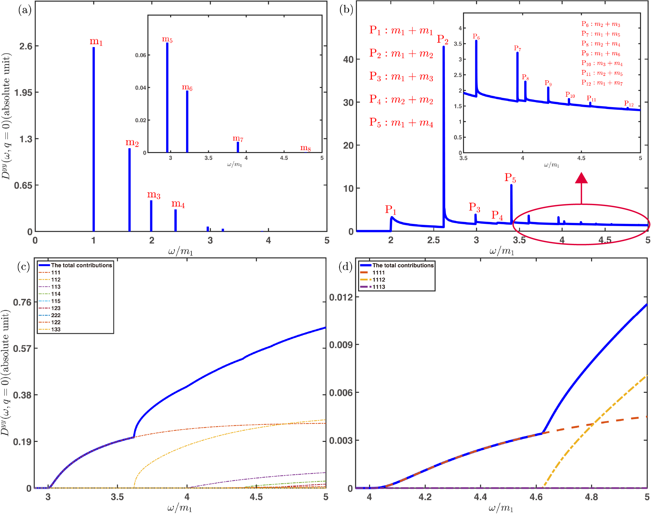
Figure 6: The analytical spectra for different particle channels’ contributions to the $D^{yy}$. Panel (a)-(d) shows the contribution from single-particle channels to four-particle channels, respectively.

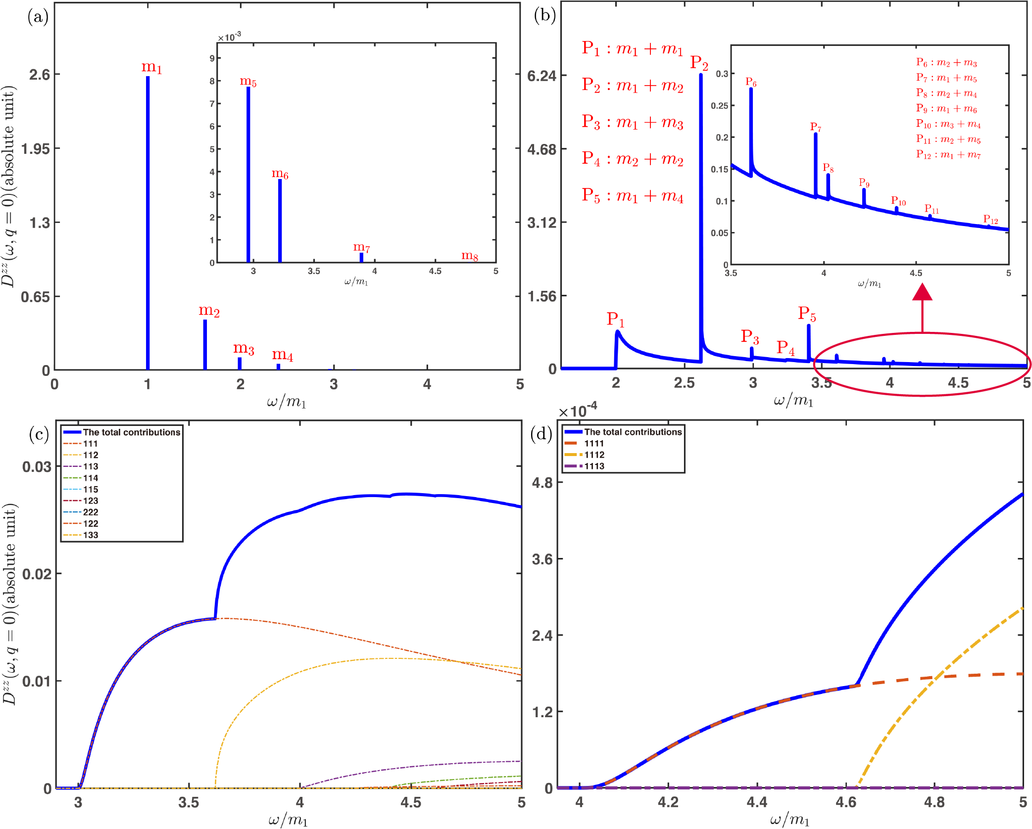
Figure 7: The analytical spectra for different particle channels’ contributions to the $D^{zz}$. Panel (a)-(d) shows the contribution from single-particle channels to four-particle channels, respectively.

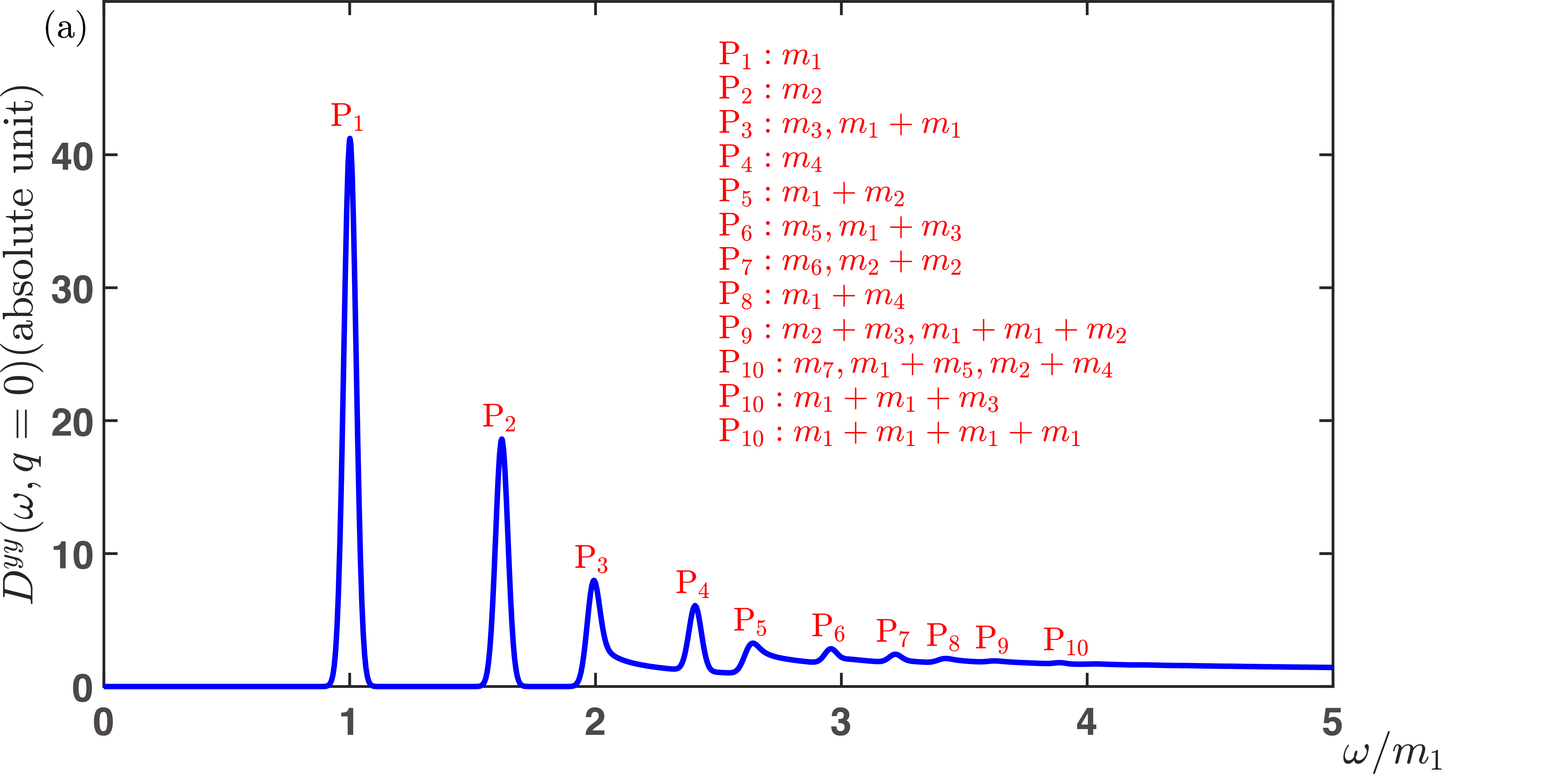
Figure 8: The total DSF of (a) $D^{yy}$ and (b) $D^{zz}$ with $0.05m_{1}$ broadening of analytical data.

References

- Sachdev (2011) S. Sachdev, Quantum Phase Transitions (Cambridge University Press, Cambridge, England, 2011).
- Belavin et al. (1984) A. Belavin, A. Polyakov, and A. Zamolodchikov, Nucl. Phys. B 241, 333 (1984).
- Zamolodchikov and Zamolodchikov (1979) A. B. Zamolodchikov and A. B. Zamolodchikov, Ann. Phys. 120, 253 (1979).
- Belavin et al. (2004) A. A. Belavin, V. A. Belavin, A. V. Litvinov, Y. P. Pugai, and A. B. Zamolodchikov, Nucl. Phys. B 676, 587 (2004).
- Delfino and Mussardo (1994) G. Delfino and G. Mussardo, Phys. Lett. B 324, 40 (1994).
- Berg et al. (1979) B. Berg, M. Karowski, and P. Weisz, Phys. Rev. D 19, 2477 (1979).
- v. Löhneysen (2010) H. v. Löhneysen, J. Low Temp. Phys. 161, 1 (2010).
- Si et al. (2001) Q. Si, S. Rabello, K. Ingersent, and J. L. Smith, Nature 413, 804 (2001).
- Coleman and Schofield (2005) P. Coleman and A. J. Schofield, Nature 433, 226 (2005).
- Schuberth et al. (2016) E. Schuberth, M. Tippmann, L. Steinke, S. Lausberg, A. Steppke, M. Brando, C. Krellner, C. Geibel, R. Yu, Q. Si, and F. Steglich, Science 351, 485 (2016).
- Wu et al. (2014) J. Wu, M. Kormos, and Q. Si, Phys. Rev. Lett. 113, 247201 (2014).
- Wang et al. (2018) Z. Wang, J. Wu, W. Yang, A. K. Bera, D. Kamenskyi, A. T. M. N. Islam, S. Xu, J. M. Law, B. Lake, C. Wu, and A. Loidl, Nature 554, 219–223 (2018).
- Wu et al. (2018) J. Wu, L. Zhu, and Q. Si, Phys. Rev. B 97, 245127 (2018).
- Wang et al. (2019) Z. Wang, M. Schmidt, A. Loidl, J. Wu, H. Zou, W. Yang, C. Dong, Y. Kohama, K. Kindo, D. I. Gorbunov, S. Niesen, O. Breunig, J. Engelmayer, and T. Lorenz, Phys. Rev. Lett. 123, 067202 (2019).
- Cui et al. (2019) Y. Cui, H. Zou, N. Xi, Z. He, Y. X. Yang, L. Shu, G. H. Zhang, Z. Hu, T. Chen, R. Yu, J. Wu, and W. Yu, Phys. Rev. Lett. 123, 067203 (2019).
- Fan et al. (2020) Y. Fan, J. Yang, W. Yu, J. Wu, and R. Yu, Phys. Rev. Research 2, 013345 (2020).
- Zamolodchikov (1989) A. B. Zamolodchikov, Int. J. Mod. Phys. A 04, 4235 (1989).
- Dorey (1997) P. Dorey, Lect. Notes Phys. 498, 85 (1997).
- Coldea et al. (2010) R. Coldea, D. A. Tennant, E. M. Wheeler, E. Wawrzynska, D. Prabhakaran, M. Telling, K. Habicht, P. Smeibidl, and K. Kiefer, Science 327, 177 (2010).
- Kjäll et al. (2011) J. A. Kjäll, F. Pollmann, and J. E. Moore, Phys. Rev. B 83, 020407 (2011).
- Zhang et al. (2020) Z. Zhang, K. Amelin, X. Wang, H. Zou, J. Yang, U. Nagel, T. Rõõm, T. Dey, A. A. Nugroho, T. Lorenz, J. Wu, and Z. Wang, Phys. Rev. B 101, 220411 (2020).
- Zou et al. (2020) H. Zou, Y. Cui, X. Wang, Z. Zhang, J. Yang, G. Xu, A. Okutani, M. Hagiwara, M. Matsuda, G. Wang, G. Mussardo, K. Hódsági, M. Kormos, Z. He, S. Kimura, R. Yu, W. Yu, J. Ma, and J. Wu, arXiv:2005.13302 (2020).
- McCoy and Wu (1978) B. M. McCoy and T. T. Wu, Phys. Rev. D 18, 1259 (1978).
- Delfino and Mussardo (1995) G. Delfino and G. Mussardo, Nucl. Phys. B 455, 724 (1995).
- Delfino and Simonetti (1996) G. Delfino and P. Simonetti, Phys. Lett. B 383, 450 (1996).
- Hódsági et al. (2019) K. Hódsági, M. Kormos, and G. Takács, J. High Energy Phys. 2019, 047 (2019).
- Schuricht and Essler (2012) D. Schuricht and F. H. L. Essler, J. Stat. Mech. (2012), eprint P04017.
- Bertini et al. (2014) B. Bertini, D. Schuricht, and F. H. L. Essler, J. Stat. Mech. (2014), eprint P10035.
- Cortés Cubero and Schuricht (2017) A. Cortés Cubero and D. Schuricht, J. Stat. Mech. (2017), eprint 103106.
- (30) See Appendix for details of the form factor bootstrap approach and the calculation of DSF.
- Amelin et al. (2020) K. Amelin, J. Engelmayer, J. Viirok, U. Nagel, T. Rõõm, T. Lorenz, and Z. Wang, Phys. Rev. B 102, 104431 (2020).
- Chaikin and Lubensky (1995) P. M. Chaikin and T. C. Lubensky, Principles of Condensed Matter Physics (Cambridge University Press, Cambridge, England, 1995).
- Pfeuty (1970) P. Pfeuty, Ann. Phys. 59, 79 (1970).
- Fateev (1994) V. A. Fateev, Phys. Lett. B 324, 45 (1994).
- (35) https://people.sissa.it/~delfino/isingff.html.
- Delfino et al. (1996) G. Delfino, P. Simonetti, and J. Cardy, Phys. Lett. B 387, 327 (1996).