Analytic Filter Function Derivatives for Quantum Optimal Control
Abstract
Auto-correlated noise appears in many solid state qubit systems and hence needs to be taken into account when developing gate operations for quantum information processing. However, explicitly simulating this kind of noise is often less efficient than approximate methods. Here, we focus on the filter function formalism, which allows the computation of gate fidelities in the presence of auto-correlated classical noise. Hence, this formalism can be combined with optimal control algorithms to design control pulses, which optimally implement quantum gates. To enable the use of gradient-based algorithms with fast convergence, we present analytically derived filter function gradients with respect to control pulse amplitudes, and analyze the computational complexity of our results. When comparing pulse optimization using our derivatives to a gradient-free approach, we find that the gradient-based method is roughly two orders of magnitude faster for our test cases. We also provide a modular computational implementation compatible with quantum optimal control packages.
I Introduction
Noise leading to the loss of quantum information remains a major challenge in the current development of quantum computers [1, 2, 3, 4]. Minimizing decoherence, while still leaving the system accessible for quantum control, stands in the center of quantum optimal control [5, 6, 7]. While quasi-static noise can be well addressed in pulse optimization approaches, treating so-called colored noise characterized, e.g., by spectral noise densities remains a difficult task [8, 9, 10, 11]. However, colored noise poses a major noise contribution in many candidate systems for quantum information processing. As such, leading solid state qubit implementations are subject to colored flux or charge noise [12, 13, 14, 15, 16, 17, 18].
The filter function formalism is a suitable and experimentally verified tool to fully describe a quantum system under wide-sense stationary classical noise with arbitrary auto- and cross-correlations [19, 20, 21, 22]. A so-called filter function quantifies the noise susceptibility of a quantum channel as a function of noise frequency. Specifically, the average gate infidelity [23, 24], a useful metric for the accuracy of quantum operations, is accessible via filter functions. Hence, this formalism can be used to design cost functions for the optimization of control pulses in the presence of correlated noise.
In previous works, colored noise has been taken into account by combining Monte Carlo simulations with Nelder-Mead optimization [25, 26]. In addition, filter function gradients have been used for quantum optimal control using gradient-based algorithms. Such algorithms typically require fewer iterations, but the overall performance gain depends on the cost of evaluating gradients. While for many problems, this cost turns out prohibitively large, it was shown that unitary quantum dynamics allow gradients to be computed rather efficiently [27]. Filter function gradients were calculated either by auto-differentiation [28] or finite differences [29]. Here, we develop analytical filter function gradients, study their computational complexity, and benchmark their application for pulse optimization. This not only allows for a numerically robust and computationally efficient implementation, but also provides insight if and when efficiency gains are expected compared to other methods. Additionally, no specialized software packages, e.g. for automatic differentiation, are required.
This paper is organized as follows: In Section II, we introduce the theoretical concepts of the filter function formalism for an easily accessible, but still non-trivial case of a single pulse of one control operator and one noise source. Subsequently, we show how to obtain the derivatives of the filter function for this case in Section III (a full but more complex derivation is presented in the appendix). We continue to introduce the numerical implementation of the derivatives in Section IV, and present an analysis of its computational complexity in Section V. In Section VI, we apply the newly implemented derivatives to pulse optimization and compare the results with a gradient-free optimization approach. We conclude in Section VII by summarizing our results and giving an outlook.
For the purpose of conciseness, we use the following notation: We denote operators and their matrix representations by Roman font, e.g. , and reserve calligraphic font for quantum operations and their representations, e.g. . Additionally, we denote the control matrix, which we will introduce in the following section, with , due to its resemblance with the Liouville representation of quantum operations. Operators in the interaction picture are written with an overset tilde, e.g. with the toggling-frame operator . Furthermore, we use an overset bar for the matrix representation of operators transformed into the eigenbasis of a Hamiltonian, e.g. with the corresponding unitary matrix of eigenvectors . A general matrix is denoted by DS font, e.g. , while its element-wise notation is labeled as . Lastly, we denote the identity matrix by , and set throughout this work.
II Filter Function Formalism for a single pulse
Before computing the derivatives, we first review the filter function formalism [24, 19, 20, 21] for the simple, but non-trivial case of a single pulse with one control operator with variable amplitude and one noise source. To this end, we break down the quantum system’s Hamiltonian into control and noise contributions, and derive the ensemble average entanglement infidelity as well as the filter function. The latter is a central quantity of the formalism and describes the quantum gate’s susceptibility to noise as a function of noise frequency. Since we focus on the infidelity, we summarize the derivation given by Green et al. [24], even though more general approaches exist [20, 21].
We start by considering a quantum system, whose total Hamiltonian during consists of two parts: a control Hamiltonian consisting of a time-independent contribution and adjustable parameters to achieve the intended quantum operation, and a noise Hamiltonian perturbing ,
| (1a) | ||||
| (1b) | ||||
Here, is a single time-dependent control amplitude with the corresponding control operator . Noise enters via the random variable and the corresponding Hermitian noise operator . The time evolution generated by the total Hamiltonian is described by the unitary operator . It is possible to rewrite the total propagator by factoring it into two parts as , where contains the control effects, and the unitary operator captures the effect of a single noise realization. While the control propagator fulfills the noise-free Schrödinger equation , it can be shown [30] that fulfills the equation of motion , with the noise Hamiltonian transformed into the interaction picture of the control Hamiltonian. The generator of can then be considered as a time-independent effective Hamiltonian , such that
| (2) |
Using the Pauli basis, can be written in terms of an error vector as . Eq. (2) can be expanded by using the Magnus expansion [31, 32], such that the exponent is given by with the first order term
| (3) |
For small noise strength, i.e. sufficiently small , higher orders provide diminishing contributions [24, 21].
A suitable measure for the quantum gate accuracy is the ensemble average entanglement infidelity [23], to which we will refer to as simply the infidelity . The infidelity is linked to via
| (4) |
By Taylor expanding the cosine term in Eq. (4), the infidelity can be approximated by for small noise . Evaluating this term only requires the square of the error vector . Inserting the first order term of the Magnus expansion given by Eq. (3) leads to
| (5) |
where is the noise amplitude’s auto-correlation function, and denotes the control matrix elements in the time domain defined by
| (6) |
where we now consider the matrix representation of the noise operator . Note that in our case of a single noise contribution, the control matrix reduces to a control vector.
Under the assumption of wide-sense stationary classical noise, the spectral noise density can be defined as the Fourier transform of . Assuming the noise to be Gaussian, which is reasonable in many cases [33], gives a full characterization of the noise. Inserting into Eq. (5) and shifting the Fourier transformation to the control matrix in frequency domain defined by
| (7) |
results in . By summing over the Cartesian coordinates, we obtain
| (8a) | ||||
| (8b) | ||||
with the filter function
| (9) |
This expression gives a full description of how the noise contribution affects the given quantum channel described by .
III Filter Function Derivatives for a single pulse
In the following, the filter function gradient with respect to the control amplitude is derived for the previously presented simple case with only a single control variable and noise contribution. To this end, we approximate for to be a sequence of piecewise-constant control amplitudes and restrict our derivation to the case of a single constant control amplitude .
Differentiating Eq. (8) requires the filter function derivative with respect to the control amplitude ,
| (10) |
By applying the product rule, the gradient of the control matrix in frequency space, , is given by the Fourier transform of
| (11) |
In order to deduce the gradient of the control propagator, , we consider a small perturbation on and add a corresponding term to the control Hamiltonian, . Let be the control propagator of the unperturbed control Hamiltonian . The perturbation Hamiltonian in the interaction picture defined by is then given by . The corresponding Schrödinger equation
| (12) |
defines the perturbation propagator . A solution of Eq. (12) can be approximated as an exponential operator by using the Magnus expansion up to first order similarly to Eqs. (2) and (3), such that
| (13a) | ||||
| (13b) | ||||
We introduce the basis change matrix consisting of the eigenvectors of the matrix representation of the control Hamiltonian , which transforms into the eigenbasis of the control Hamiltonian and indicate an operator in matrix representation under such a transformation as . Since , inserting the identity into the exponent given by Eq. (13b) leads to
| (14) |
Naturally, the control propagator in the eigenbasis of the control Hamiltonian is diagonal. Specifically, if we consider the sorted set of eigenvalues of the control Hamiltonian in the same order as the eigenvectors in , it is given by . For the further calculation, we introduce the element-wise notation for the matrix . The integral in Eq. (14) can then be evaluated as
| (15a) | ||||
| (15b) | ||||
| (15c) | ||||
where is the Kronecker delta. We now notice that the total propagator of is given by , and that . Using this, we can rewrite the control propagator derivative as
| (16) |
In order to calculate , we differentiate Eq. (13a) to first order. To this end, we need to take the derivative of the exponent given by Eq. (14). Taking into account Eq. (15) and recognizing that
| (17) |
the derivative of the exponent is given by
| (18) |
where symbolizes element-wise multiplication. Considering Eqs. (13) - (18), the derivative of the control propagator with respect to the constant control amplitude can be calculated as
| (19) |
By inserting Eq. (19) into Eq. (11) and the latter equation into Eq. (10), we have derived a complete analytic form of the filter function gradient for the considered case of a single pulse.
In general, a pulse sequence can consist of several time steps, control contributions, and noise sources. Under the assumption of piecewise-constant control amplitudes, the total control effect on the quantum system is a composition of the single pulse effects. The total control matrix is then given by [21, 20]
| (20) |
where are the single pulse control matrices given by Eqs. (6) and (7), and are the cumulative control propagators of the individual single pulses, i.e. the control propagators in Liouville representation multiplied with each other up to each time step. A more detailed explanation is given in Appendix A. Consequently, when calculating filter function gradients for a general pulse sequence, products of in the total control matrix need to be taken into account in Eq. (10). To this end, partial derivatives of the cumulative control propagators of the individual pulses have to be deduced additionally. A full calculation of the filter function gradient for a generic pulse sequence is given in Appendix B.
IV Software Implementation
We implemented the filter function gradients derived in the previous section as part of the open source software framework filter_functions [34, 21]. This python package facilitates the efficient numerical calculation of generalized filter functions and derived quantities, such as the infidelity, for given pulse sequences. A pulse sequence is represented by the PulseSequence class, from which properties like the filter function or infidelity can directly be computed. The newly implemented module gradient enables the calculation of filter function and infidelity derivatives for systems that are subject to classical wide-sense stationary noise, which can be characterized by an arbitrary spectral noise density. The gradients are taken with respect to stepwise constant control amplitudes. The function infidelity_derivative() is placed at the user’s disposal for direct calculation of the infidelity derivatives for a given pulse sequence. This function can be used directly for quantum optimal control, i.e. to optimize gate fidelities. An illustration of the structure of the implementation can be found in Appendix C, and a verification of the implemented analytical gradients are available in Ref. 21. Furthermore, we ensured the implementation’s compatibility with quantum optimal control packages, such as qopt [35, 36].
V Computational Complexity
In principle, our software implementation enables the calculation of filter function and infidelity gradients without any constraints on the quantum system’s dimension or on the number of control and noise operators and . Furthermore, a pulse sequence can contain any number of time steps and the number of frequency samples describing the noise spectral density is completely variable. Naturally, the computational complexity in computing the infidelity derivatives depends on the chosen set of parameters. Theoretical investigations of the implementation lead to the expected scaling behavior summarized in Table 1 for dominant terms.
| Parameter | Expectation | Run Time |
|---|---|---|
| Number of frequency samples | ||
| Number of control operators | ||
| Number of noise operators | ||
| Number of time steps | ||
| Dimension | 111 arises from the multiplication of two -matrices, which scales polynomially with . For a naive algorithm [37] and for the Coppersmith–Winograd algorithm [38]. |
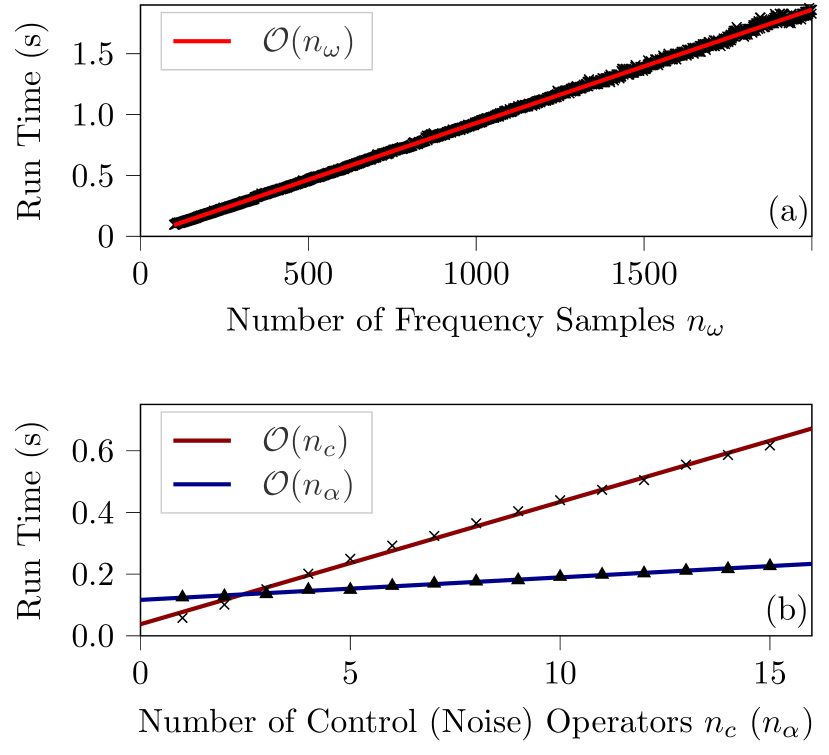
We analyze the actual run time behavior by running the implemented software module with various pulses. To this end, we increase one of the parameters , , , and , while fixing the remaining quantities and generating the control amplitudes randomly for each pulse. We then obtain the scaling behavior of the implementation by means of asymptotic fits. A graphical illustration can be seen in Fig. 3 and in Appendix C. Table 1 contrasts the actual run time results with their theoretical expectations.

The plots confirm the expected linear dependence on , and . For various and , the run time data is shown in Fig. 3. A polynomial fit on the data for various stands in agreement with the expectation of quadratic scaling. Concerning the -dependency, a clear polynomial behavior is visible. Due to memory limitation, we tested dimensions restricted to . Within this restriction, lower order terms in dominate the scaling behavior, such that this cannot be considered as an asymptotic regime. Therefore, the underestimated exponent for the -dependency does not contradict the theoretical expectation.
VI Application
As mentioned previously, filter function derivatives lend themselves to gradient-based pulse optimization. In the following, we motivate the use of such gradient-based methods by comparing the numerical optimization of control pulses using filter function gradients to a gradient-free approach.
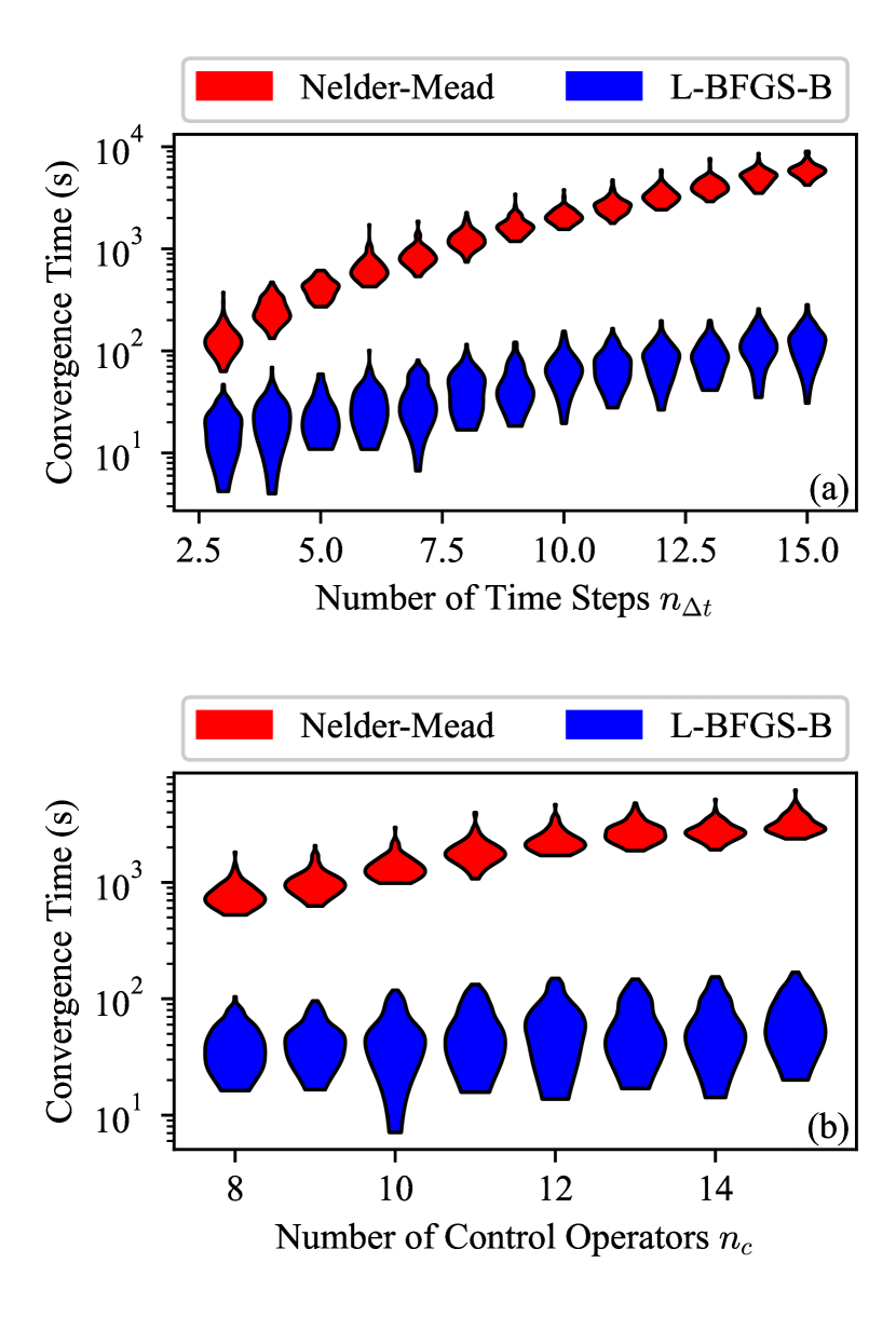
To this end, we use the filter function derivatives in conjunction with scipy’s L-BFGS-B algorithm [39, 40] and contrast this strategy with a gradient-free constrained Nelder-Mead method [41, 42] in terms of run time and error rates of the optimized pulses. We conduct both optimization approaches within the quantum optimal control package qopt [35, 36]. To facilitate a fair comparison, we disabled the internal multi-threading of the optimization algorithms in python.
We apply each technique to a generic 4-level quantum system corresponding to the optimization of two-qubit gates. For this purpose, we use a control Hamiltonian given by
| (21) |
where signifies the piecewise constant control amplitudes at the discrete time step of uniform length . For simplicity, we assume the system to be exposed to exactly one noise source, such that the noise Hamiltonian is given by . In the latter, denotes a noise amplitude corresponding to a pink noise spectral density of the form with frequency and constant .
We choose the cost function of the pulse optimization to be the total infidelity , which is the sum of systematic and noise-induced deviations from the target gate. The former ones are quantified by the standard entanglement infidelity and the latter ones are calculated as in Eq. (8). The optimization problem then lies in the minimization of the infidelity by finding the optimal control amplitudes .
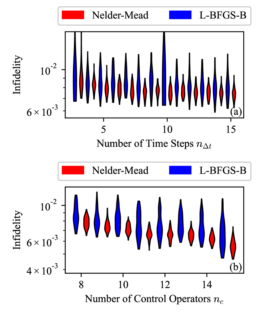
As convergence criterion, we choose that improves by less than within one iteration of the optimization algorithm, which does not favor either algorithm (see Fig. 6 in Appendix D). The performance is depicted in Fig. 2, where we observe that the L-BFGS-B algorithm converges faster and scales better with the number of time steps and the number of control operators . Both algorithms find locally optimal pulses with similar fidelities (see Fig. 5 in Appendix D).
In Appendix B, we discuss the convergence of the two optimization algorithms in greater detail, demonstrating that the Nelder-Mead algorithm offers better global performance, while the L-BFGS-B algorithm is more prone to get stuck in local minima. A further discussion of the benefits of filter functions compared to Monte Carlo methods and the description of open quantum systems by master equations can be found in Ref. 36.
VII Conclusion and Outlook
In this paper, we presented analytically derived filter function gradients and their numerical implementation. By doing so, we make the gradients easily accessible for various pulse optimization algorithms. Furthermore, we conducted an analysis of the computational complexity for obtaining the filter function derivatives by our implementation. We verified the theoretical prediction by comparing them to the actual run time scaling behavior. Finally, we applied our filter function derivatives to gradient-based pulse optimization of generic two-qubit gates and contrast this approach with a gradient-free optimization method. While both strategies result in optimized pulses of similar fidelities, we showed that the gradient-based optimization requires up to two orders of magnitude less time to converge than the gradient-free optimization for our test case.
In addition to pulse optimization for implementation of quantum gates, various other applications for analytic filter function derivatives exist. Since the filter function formalism can be used to describe quantum algorithms in terms of pulse sequences [20, 21], filter function gradients can not only be used to optimize quantum gates, but also the implementation of quantum algorithms. Furthermore, pulse optimization can also aid noise spectroscopy [43], where carefully designed control pulses are used to obtain an accurate description of the present spectral noise density. As another application, filter function derivatives could be used to assess the impact of quasistatic noise or calibration errors on the high-frequency noise properties of a given pulse. Lastly, if the noise environment changes, e.g. due to dynamically changing operational parameters of on-chip control electronics, our gradients can be used to quickly re-calibrate qubits in a quantum processor.
Based on our results analytic filter function derivatives can facilitate quantum optimal control for various proposed qubit implementations that are subject to arbitrary classical auto- and cross-correlated noise. Thus, these derivatives can help to assess the potential performance of candidate hardware platforms for quantum information processing [44, 45, 46].
Acknowledgements.
This work is supported by the European Research Council (ERC) under the European Union’s Horizon 2020 research and innovation program (Grant Agreement No. 679342). All correspondence should be addressed to Hendrik Bluhm.Appendix A Filter function formalism for a general pulse sequence
In Section II of the main paper, the filter function formalism has been presented for the special case of a single control contribution and a single noise source. The following section recaptures some modifications needed for the calculation of filter function derivatives of a general pulse sequence consisting of various control and noise contributions.
Consider now the general description of a quantum system, whose total Hamiltonian during consists of two parts: a control Hamiltonian consisting of a time-independent contribution and multiple adjustable parameters to achieve the intended quantum operation, and a noise Hamiltonian perturbing ,
| (22a) | ||||
| (22b) | ||||
| (22c) | ||||
Within , is the adjustable control strength of the control operator at time . Likewise in , is the randomly distributed amplitude of the Hermitian noise operator and captures the system’s sensitivity to the corresponding noise source and might be dependent on the control amplitude.
Following the approach given in Section II, the control matrix can be derived. The control propagator again contains the control effects and fulfills the noise-free Schrödinger equation . In the main paper, the set of Pauli operators was chosen as an operator basis. In general, the operators can be expressed in any orthonormal operator basis with respect to the Hilbert-Schmidt product . Taking this generalization into account, and considering the noise sensitivity, the control matrix in time domain needs to be modified. It is then defined as
| (23) |
In case of piecewise constant control, a control sequence consists of constant single pulses. Let us denote as the time interval corresponding to the th single pulse for . The control sequence can then be described with help of the single pulse propagators . Consequently, the propagator cumulated up to the th time step is given by and its so-called Liouville representation is defined by . Next, we denote the duration of the th single pulse with , and the single pulse control matrix in frequency space at time step with
| (24) |
The total control matrix of the pulse sequence can then be directly determined by
| (25) |
In the above, is the control propagator of the individual single pulses cumulated up to time step . The temporal positions of the single pulses enter the expression due to the Fourier transform via the phase factor . Therefore, it is possible to obtain the total control matrix of a generic pulse sequence by summing up each single pulse control matrix multiplied with the cumulated control propagators of the priorly executed single pulses. Using Eq. (25), the filter function for a noise contribution can be obtained by Eq. (9). If we extend the calculation to generic dimensions , the infidelity for a noise contribution is given by
| (26) |
Appendix B Filter function derivatives for a general pulse sequence
When considering a pulse sequence with time steps, the correlation terms in the total control matrix given by Eq. (20) need to be taken into account. In the following, we derive the filter function gradient for the general case of a pulse sequence under the assumption of piecewise-constant control.
We write for the control amplitude in direction at a fixed time and note that for . Applying the product rule on Eq. (25) results in
| (27) | ||||
This expression depends on four quantities: the control propagators in Liouville representation , and their partial derivatives ; and the control matrices , and their partial derivatives . To break the calculation into comprehensive parts, we dedicate each of the mentioned quantities one of the following subsections.
B.1 Control matrix at time step
For a fixed time step , the single control matrix is defined in Eq. (24). In the following, we will evaluate the integral formula analytically. To this end, we introduce the basis change matrix with its columns being the eigenvectors of the control Hamiltonian at time step , . An operator in matrix representation transformed into the eigenbasis of is then denoted by .
Let be the set of eigenvalues of in the same order as the eigenvectors in . The control propagator during time step transformed into the eigenbasis of is naturally a diagonal matrix
| (28) |
with . Due to piecewise constant control, the sensitivity during the th time step is constant, i.e. . Inserting the identity into Eq. (23), and taking into account the cyclic properties of the trace results in
| (29a) | ||||
| (29b) | ||||
| (29c) | ||||
Now we can carry out the transformation of into frequency domain given by Eq. (24). Since and are not time-dependent, evaluating the time integral over time dependent factors at time step yields
| (30a) | ||||
| (30b) | ||||
By inserting this expression into Eq. (24) and denoting element-wise multiplication by , the control matrix in frequency space can be evaluated to
| (31a) | ||||
| (31b) | ||||
B.2 Derivative of the control propagator
In the main paper we have already derived a closed formula of the control propagator gradient in the case of a single pulse. The resulting expression in Eq. (19) is valid for each control propagator gradient within a certain time step . More specifically, the derivative of the control propagator within time step is given as
| (32) |
The difference is that in the general case, various control contributions are considered, and that and denote each quantity for the specific considered time step .
B.3 Derivative of the propagator in Liouville representation
The main difference between the cases of a single pulse and a pulse sequence is that we need to take the derivative of the cumulated control propagator in Liouville representation at each time step into account. To this end, we keep in mind that is the cumulative propagator up to time step and that its Liouville representation is given element-wise as . For the further calculation we first need the derivative of , which can be evaluated as
| (33a) | |||
| (33b) |
where Eq. (33b) incorporates the fact that cumulative propagators up to a time step are independent of the control at a later point in time and where given by Eq. (32). By applying the product rule, we calculate the derivative of element-wise to
| (34) |
B.4 Derivative of the control matrix
The last quantity that remains to be computed are the derivatives of single control matrices. In order to calculate the derivative of the control matrix at time step in the frequency domain , we will first obtain a formula for the gradient in time space and subsequently transform the result into frequency space. To this end, we consider and again label . If depends on the control amplitudes, an additive term including the noise sensitivity derivative needs to be taken into account. Here, we assume to know the analytic dependency of on the control amplitudes and therefore, concentrate on the remaining term by choosing to be independent of the control amplitudes. Using the product rule and cyclic properties of the trace, and keeping in mind that the noise and control operators are independent of the control strength leads to
| (35) |
where we write for the commutator of and .
Similarly to the approach in Section B.1, we transform the control propagator into the eigenspace of and make use of its diagonal form given in Eq. (28). Under consideration of the cyclic properties of a trace, and writing , the calculation can be further carried out as
| (36) |
Transforming the latter into frequency domain requires an integration over time. Since and are time-independent within the regarded time step, this integration lies in
| (37a) | ||||
| if and | ||||
| (37b) | ||||
| otherwise. | ||||
Using this result, we can first evaluate the transformed commutator element-wise to
| (38) |
and consequently derive a concise formula for the gradient of the control matrix at time step in the frequency domain as
| (39) |
Appendix C Supplement information on software implementation and computational complexity
C.1 Structure of implementation
In order to extend the filter_functions software package by filter function derivatives, the module gradient was implemented. Additionally, a method for directly obtaining filter function derivatives from a given pulse sequence was added to the PulseSequence class. The overall structure is illustrated in Fig. 3.

C.2 Verification of linear run time dependency
Within the run time analysis, the theoretically predicted linear dependency on the number of frequency samples, control operators, and noise operators could clearly be verified by means of asymptotic plots. Figure 4 displays the analysis’ results.
Appendix D Supplement information on the comparison to Nelder-Mead method
In the following we will elaborate more on the details of the optimizations used to compare the use analytical gradients to a gradient free method. For better comparability, both optimization algorithms were started from the same initial pulses.
In Fig. 5 we plotted the distribution of the optimized pulses’ infidelities found in the optimization corresponding to Fig. 2. We can see that both algorithms find similar minimal infidelities over 100 runs. From the fact that the distribution of final cost values is wider for the L-BFGS-B algorithm, we can deduct that the gradient based method is more prone to get stuck in local minima in the optimization space, while the Nelder-Mead algorithm appears to provide better global convergence.
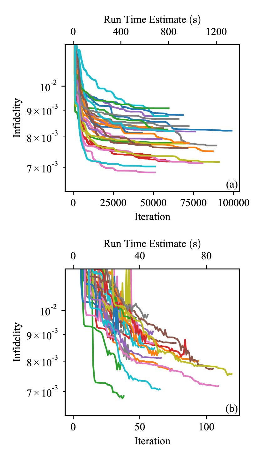
In the convergence plots in Fig. 6, it can be seen that the gradient-based method requires far less iterations than the Nealder-Mead algorithm. The plateaus in the plots, where the algorithm reduces the Infidelity only marginally over several iterations, can be interpreted as features in the optimization landscape with the approximate form of local minima. We also observe, that the termination condition favors neither algorithm as both do not spend an excessive amount of iterations for minor improvements.
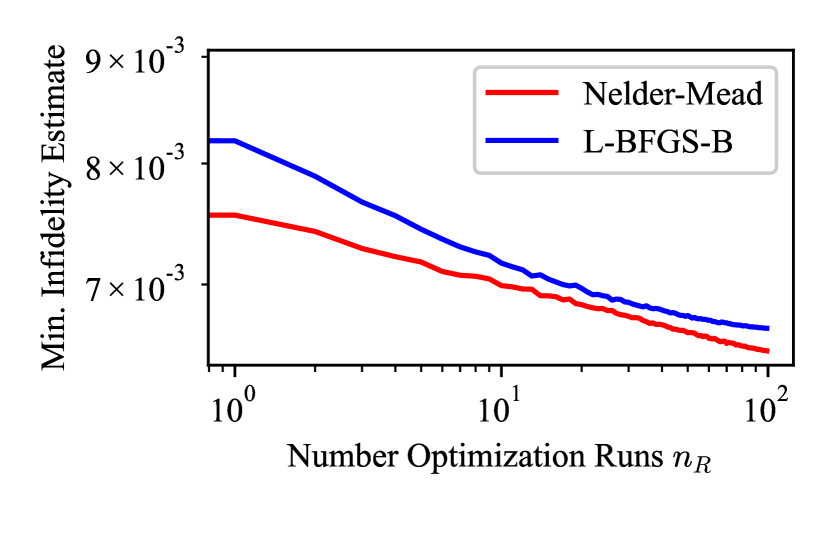
To compare the convergence of the algorithms with respect to the initial parameters, we plotted in Fig. 7 the expectation value of the infidelity as function of the number of optimization runs . This quantifies the infidelity of the best pulse found by starting the optimization times with different initial pulse values. To find a pulse of similar infidelity on average, the L-BFGS-B algorithm needs to be restarted roughly twice as many times as the Nelder-Mead algorithm.
References
- Nielsen and Chuang [2010] M. A. Nielsen and I. L. Chuang, Quantum Computation and Quantum Information (Cambridge University Press, 2010).
- Harrow and Montanaro [2017] A. W. Harrow and A. Montanaro, Quantum computational supremacy, Nature 549, 203 (2017).
- Unruh [1995] W. G. Unruh, Maintaining coherence in quantum computers, Phys. Rev. A 51, 992 (1995).
- Preskill [2018] J. Preskill, Quantum Computing in the NISQ era and beyond, Quantum 2, 79 (2018).
- Glaser et al. [2015] S. J. Glaser, U. Boscain, T. Calarco, C. P. Koch, W. Köckenberger, R. Kosloff, I. Kuprov, B. Luy, S. Schirmer, T. Schulte-Herbrüggen, D. Sugny, and F. K. Wilhelm, Training Schrödinger’s cat: Quantum optimal control: Strategic report on current status, visions and goals for research in Europe, Eur. Phys. J. D 69, 279 (2015).
- Peirce et al. [1988] A. P. Peirce, M. A. Dahleh, and H. Rabitz, Optimal control of quantum-mechanical systems: Existence, numerical approximation, and applications, Phys. Rev. A 37, 4950 (1988).
- Rabitz [2009] H. Rabitz, Focus on Quantum Control, New J. Phys 11, 105030 (2009).
- Wang et al. [2012] X. Wang, L. S. Bishop, J. P. Kestner, E. Barnes, K. Sun, and D. Sarma, Composite pulses for robust universal control of singlet-triplet qubits, Nat. Commun. 3, 997 (2012).
- Wang et al. [2014a] X. Wang, L. S. Bishop, E. Barnes, J. P. Kestner, and S. D. Sarma, Robust quantum gates for singlet-triplet spin qubits using composite pulses, Phys. Rev. A 89, 022310 (2014a).
- Wang et al. [2014b] X. Wang, F. A. Calderon-Vargas, M. S. Rana, J. P. Kestner, E. Barnes, and S. Das Sarma, Noise-compensating pulses for electrostatically controlled silicon spin qubits, Phys. Rev. B 90, 155306 (2014b).
- Yang and Wang [2016] X. C. Yang and X. Wang, Noise filtering of composite pulses for singlet-triplet qubits, Sci. Rep. 6, 28996 (2016).
- Wellstood et al. [1987] F. C. Wellstood, C. Urbina, and J. Clarke, Low‐frequency noise in dc superconducting quantum interference devices below 1 k, Appl. Phys. Lett. 50, 772 (1987).
- Bylander et al. [2011] J. Bylander, S. Gustavsson, F. Yan, F. Yoshihara, K. Harrabi, G. Fitch, D. G. Cory, Y. Nakamura, J. S. Tsai, and W. D. Oliver, Noise spectroscopy through dynamical decoupling with a superconducting flux qubit, Nat. Phys. 7, 565 (2011).
- Drung et al. [2011] D. Drung, J. Beyer, J. Storm, M. Peters, and T. Schurig, Investigation of low-frequency excess flux noise in dc squids at mk temperatures, IEEE Trans. Appl. Supercond. 21, 340 (2011).
- Anton et al. [2012] S. M. Anton, C. Müller, J. S. Birenbaum, S. R. O’Kelley, A. D. Fefferman, D. S. Golubev, G. C. Hilton, H.-M. Cho, K. D. Irwin, F. C. Wellstood, G. Schön, A. Shnirman, and J. Clarke, Pure dephasing in flux qubits due to flux noise with spectral density scaling as , Phys. Rev. B 85, 224505 (2012).
- Kuhlmann et al. [2013] A. V. Kuhlmann, J. Houel, A. Ludwig, L. Greuter, D. Reuter, A. D. Wieck, M. Poggio, and R. J. Warburton, Charge noise and spin noise in a semiconductor quantum device, Nat. Phys. 9, 570 (2013).
- Yoneda et al. [2018] J. Yoneda, K. Takeda, T. Otsuka, T. Nakajima, M. R. Delbecq, G. Allison, T. Honda, T. Kodera, S. Oda, Y. Hoshi, N. Usami, K. M. Itoh, and S. Tarucha, A quantum-dot spin qubit with coherence limited by charge noise and fidelity higher than 99.9%, Nat. Nanotechnol. 13, 102 (2018).
- Struck et al. [2020] T. Struck, A. Hollmann, F. Schauer, O. Fedorets, A. Schmidbauer, K. Sawano, H. Riemann, N. V. Abrosimov, Ł. Cywiński, D. Bougeard, and L. R. Schreiber, Low-frequency spin qubit energy splitting noise in highly purified 28Si/SiGe, npj Quantum Inf. 6, 40 (2020).
- Green et al. [2013] T. J. Green, J. Sastrawan, H. Uys, and M. J. Biercuk, Arbitrary quantum control of qubits in the presence of universal noise, New J. Phys. 15, 095004 (2013).
- Cerfontaine et al. [2021] P. Cerfontaine, T. Hangleiter, and H. Bluhm, Filter functions for quantum processes under correlated noise (2021), arXiv:2103.02385 [quant-ph] .
- Hangleiter et al. [2021a] T. Hangleiter, P. Cerfontaine, and H. Bluhm, Filter function formalism and software package to compute quantum processes of gate sequences for classical non-markovian noise (2021a), arXiv:2103.02403 [quant-ph] .
- Soare et al. [2014] A. Soare, H. Ball, D. Hayes, J. Sastrawan, M. C. Jarratt, J. J. Mcloughlin, X. Zhen, T. J. Green, and M. J. Biercuk, Experimental noise filtering by quantum control, Nat. Phys. 10, 825 (2014).
- Nielsen [2002] M. A. Nielsen, A simple formula for the average gate fidelity of a quantum dynamical operation, Phys. Lett. A 303, 249 (2002).
- Green et al. [2012] T. Green, H. Uys, and M. J. Biercuk, High-order noise filtering in nontrivial quantum logic gates, Phys. Rev. Lett. 109, 020501 (2012).
- Huang and Goan [2017] C.-H. Huang and H.-S. Goan, Robust quantum gates for stochastic time-varying noise, Phys. Rev. A 95, 062325 (2017).
- Huang et al. [2019] C.-H. Huang, C.-H. Yang, C.-C. Chen, A. S. Dzurak, and H.-S. Goan, High-fidelity and robust two-qubit gates for quantum-dot spin qubits in silicon, Phys. Rev. A 99, 042310 (2019).
- Kuprov and Rodgers [2009] I. Kuprov and C. T. Rodgers, Derivatives of spin dynamics simulations, J. Chem. Phys. 131, 234108 (2009).
- Ball et al. [2020] H. Ball, M. J. Biercuk, A. Carvalho, J. Chen, M. Hush, L. A. D. Castro, L. Li, P. J. Liebermann, H. J. Slatyer, C. Edmunds, V. Frey, C. Hempel, and A. Milne, Software tools for quantum control: Improving quantum computer performance through noise and error suppression (2020), arXiv:2001.04060 [quant-ph] .
- Cerfontaine et al. [2014] P. Cerfontaine, T. Botzem, D. P. DiVincenzo, and H. Bluhm, High-fidelity single-qubit gates for two-electron spin qubits in GaAs, Phys. Rev. Lett. 113, 150501 (2014).
- Haeberlen and Waugh [1968] U. Haeberlen and J. S. Waugh, Coherent averaging effects in magnetic resonance, Phys. Rev. 175, 453 (1968).
- Blanes et al. [2009] S. Blanes, F. Casas, J. A. Oteo, and J. Ros, The Magnus expansion and some of its applications, Phys. Rep. 470, 151 (2009).
- Magnus [1954] W. Magnus, On the exponential solution of differential equations for a linear operator, Commun. Pure. Appl. Math. 7, 649 (1954).
- Szańkowski et al. [2017] P. Szańkowski, G. Ramon, J. Krzywda, D. Kwiatkowski, and Ł. Cywiński, Environmental noise spectroscopy with qubits subjected to dynamical decoupling, J. Phys. Condens. Matter 29, 333001 (2017).
- Hangleiter et al. [2021b] T. Hangleiter, I. N. M. Le, and J. D. Teske, filter_functions: A package for efficient numerical calculation of generalized filter functions to describe the effect of noise on quantum gate operations (version v1.0.0), https://doi.org/10.5281/zenodo.4575001 (2021b).
- Teske [2021] J. Teske, qopt: A simulation and quantum optimal control package, https://github.com/qutech/qopt (2021).
- Teske et al. [2020] J. Teske, P. Cerfontaine, and H. Bluhm, qopt: A qubit simulation and quantum optimal control package (2020), in preparation.
- Cormen et al. [2009] T. H. Cormen, C. E. Leiserson, R. L. Rivest, and C. Stein, Introduction to Algorithms, 3rd ed. (The MIT Press, 2009).
- Coppersmith and Winograd [1990] D. Coppersmith and S. Winograd, Matrix multiplication via arithmetic progressions, J. Symb. Comput. 9, 251 (1990).
- Zhu et al. [1997] C. Zhu, R. H. Byrd, P. Lu, and J. Nocedal, Algorithm 778: L-bfgs-b: Fortran subroutines for large-scale bound-constrained optimization, ACM Trans. Math. Softw. 23, 550–560 (1997).
- Morales and Nocedal [2011] J. L. Morales and J. Nocedal, Remark on “algorithm 778: L-bfgs-b: Fortran subroutines for large-scale bound constrained optimization”, ACM Trans. Math. Softw. 38, 7 (2011).
- Nelder and Mead [1965] J. A. Nelder and R. Mead, A Simplex Method for Function Minimization, Comput. J. 7, 308 (1965).
- [42] A. Blaessle, constrnmpy: Constrained nealder mead implemented in python.
- Pozza et al. [2019] N. D. Pozza, S. Gherardini, M. M. Müller, and F. Caruso, Role of the filter functions in noise spectroscopy, Int. J. Quantum Inf. 17, 1941008 (2019).
- Kelly et al. [2014] J. Kelly, R. Barends, B. Campbell, Y. Chen, Z. Chen, B. Chiaro, A. Dunsworth, A. G. Fowler, I.-C. Hoi, E. Jeffrey, A. Megrant, J. Mutus, C. Neill, P. J. J. O’Malley, C. Quintana, P. Roushan, D. Sank, A. Vainsencher, J. Wenner, T. C. White, A. N. Cleland, and J. M. Martinis, Optimal quantum control using randomized benchmarking, Phys. Rev. Lett. 112, 240504 (2014).
- Cerfontaine et al. [2020] P. Cerfontaine, T. Botzem, J. Ritzmann, S. S. Humpohl, A. Ludwig, D. Schuh, D. Bougeard, A. D. Wieck, and H. Bluhm, Closed-loop control of a GaAs-based singlet-triplet spin qubit with 99.5% gate fidelity and low leakage, Nature Communications 11, 4144 (2020).
- Biercuk et al. [2009] M. J. Biercuk, H. Uys, A. P. VanDevender, N. Shiga, W. M. Itano, and J. J. Bollinger, High-fidelity quantum control using ion crystals in a penning trap (2009), arXiv:0906.0398 [quant-ph] .