Distributed motion coordination for multi-robot systems under LTL specifications

Pian Yu and Dimos V. Dimarogonas This work was supported in part by the Swedish Research Council (VR), the Swedish Foundation for Strategic Research (SSF) and the Knut and Alice Wallenberg Foundation (KAW).The authors are with School of Electrical Engineering and Computer Science, KTH Royal Institute of Technology, 10044 Stockholm, Sweden. piany@kth.se, dimos@kth.se
Abstract

This paper investigates the online motion coordination problem for a group of mobile robots moving in a shared workspace, each of which is assigned a linear temporal logic specification. Based on the realistic assumptions that each robot is subject to both state and input constraints and can have only local view and local information, a fully distributed multi-robot motion coordination strategy is proposed. For each robot, the motion coordination strategy consists of three layers. An offline layer pre-computes the braking area for each region in the workspace, the controlled transition system, and a so-called potential function. An initialization layer outputs an initially safely satisfying trajectory. An online coordination layer resolves conflicts when one occurs. The online coordination layer is further decomposed into three steps. Firstly, a conflict detection algorithm is implemented, which detects conflicts with neighboring robots. Whenever conflicts are detected, a rule is designed to assign dynamically a planning order to each pair of neighboring robots. Finally, a sampling-based algorithm is designed to generate local collision-free trajectories for the robot which at the same time guarantees the feasibility of the specification. Safety is proven to be guaranteed for all robots at any time. The effectiveness and the computational tractability of the resulting solution is verified numerically by two case studies.

Index Terms:
Multi-robot systems; motion coordination; safety; distributed control; constraints.

I Introduction

One challenge for multi-robot systems (MRSs) is the design of coordination strategies between robots that enable them to perform operations safely and efficiently in a shared workspace while achieving individual/group motion objectives [1]. This problem was originated from the 80s and has been extensively investigated since. In recent years, the attention that has been put on this problem has grown significantly due to the emergence of new applications, such as smart transportation and service robotics. The existing literature can be divided into two categories: path coordination and motion coordination. The former category plans and coordinates the entire paths of all the robots in advance (offline), while the latter category focuses on decentralized and online approaches that allow robots to resolve conflicts online when one occurs111In some literature these two terms are used interchangeably. In this paper, we try to distinguish between the two as explained above. [2]. This paper aims at developing a fully distributed strategy for multi-robot motion coordination (MRMC) with safety guarantees.

Depending on how the controller is synthesized for each robot, the literature concerning MRMC can be further classified into two types: the reactive approach and the planner-based approach. Typical methods that generate reactive controllers consist of the potential-field approach [3, 4], sliding mode control [5, 6] and control barrier functions [7, 8]. These reactive-style methods are fast and operate well in real-time. However, it is well-known that these methods are sensitive to deadlocks that are caused by local minima. Moreover, although these reactive-style methods work well in relatively unconstrained situations, guidance for setting control parameters is not analyzed formally when explicit constraints on the system states and/or inputs are presented [2]. Apart from the above, other reactive methods include the generalized roundabout policy [9] and a family of biologically inspired methods [10].

An early example of the planner-based method is the work of Azarm and Schmidt [11], where a framework for online coordination of multiple mobile robots was proposed. In this framework, MRMC was solved as a sequential trajectory planning problem, where priorities are assigned to robots when conflicts are detected, and then a motion planning algorithm is implemented to generate conflict-free paths. Based on this framework, various applications and different motion planning algorithms are investigated. Guo and Parker [12] proposed a MRMC strategy based on the D algorithm. In this work, each robot has an independent goal position to reach and know all path information. In [13], a distributed bidding algorithm was designed to coordinate the movement of multiple robots, which focuses on area exploration. In the work of Liu [14], conflict resolution at intersections was considered for connected autonomous vehicles, where each vehicle is required to move along a pre-planned path. A literature review on MRMC can be found in [1].

No matter which type of controllers is implemented, safety has always been a crucial issue for MRMC. In [7], MRSs with double-integrator dynamics were studied, control barrier functions were proposed to solve the motion coordination problem and safety guarantees were established. However, the velocity constraints are not dealt with. In [14], safety was stated by assuming that the deceleration that each robot can take is unbounded, yet this assumption may not be realistic for practical applications. In addition, most of the above mentioned literature concerning MRMC considers relatively simple tasks for each robot (e.g., an arrival task from initial state to goal state). However, as robots become more capable, a recent trend in the area of robot motion planning is to assign robots more complex, high-level tasks, such as temporal logic specifications.

In the last few years, multi-robot control under linear temporal logic (LTL) specifications has been investigated in [15, 16, 17, 18, 19, 20]. Most of them consider that the MRS is subject to a global LTL specification, and then an offline motion planning problem is solved in a centralized manner [15, 16, 17, 18]. In [19], unknown moving obstacles were taken into account. Therefore, online coordination with the moving obstacles was further required. In this work, safety is shown under the assumptions that each robot is moving at a constant velocity and that the local motion planning is feasible. In [20], multi-robot plan reconfiguration under local LTL specifications was investigated. A potential-field-based navigation controller was implemented for each robot to guarantee safety. However, the approach is not applicable when state and input constraints are considered.

Motivated by the above observations, this paper investigates the MRMC problem for a group of mobile robots moving in a shared workspace, each of which is assigned a LTL specification. Robots are assumed to have limited sensing capabilities and constraints in both state and input are considered. To cope with these setups, a fully distributed MRMC strategy is proposed. The contributions of this paper are summarized as follows.

  • i)

    A framework for distributed MRMC under LTL specifications is proposed for each robot, which consists of three layers: an offline pre-computation layer, an initialization layer, and an online coordination layer. The online coordination layer is further decomposed into three steps. Firstly, conflicts are detected within the sensing area of each robot. Once conflicts are detected, a rule is applied to assign dynamically a planning order to each pair of neighboring robots. Finally, a sampling-based algorithm is implemented for each robot that generates a local collision-free trajectory which at the same time satisfies the LTL specification.

  • ii)

    Safety is established under all circumstances by combining the planner-based controller with an emergency braking controller.

  • iii)

    As the motion coordination strategy is designed to be fully distributed and each robot considers only local information of neighboring robots, it is totally scalable in the sense that the computational complexity of the strategy does not increase with the number of robots in the workspace.

A comparison between this work and the related literature [15, 16, 17, 18, 20, 19] is summarized in Table I.

[b] Literature Task1 Plan synthesis Online coordination Safety2 [15, 16, 17, 18] global centralized no offline safety [19] global centralized yes additional assumptions [20] local distributed yes no state and input constraints are considered This work local distributed yes no additional assumptions, state and input constraints are considered

TABLE I: Comparison of this work to related literature.
  • 1

    Global means that a team LTL specification is assigned to all robots, local means that an individual LTL specification is assigned to each robot.

  • 2

    Safety means robot-robot and robot-obstacle collision avoidance.

A preliminary version of this work was accepted by the 2020 American Control Conference [21]. Here, we expand this preliminary version in two main directions. Firstly, the framework is generalized to LTL specifications. In the conference version, only reach-avoid type of tasks are considered, and the replanning problem can be formulated as an optimization problem. However, as the verification of an LTL formula is in general difficult to be conducted online, a local trajectory generation algorithm is designed in this work. Secondly, safety guarantees are established without the assumption that each robot can take unbounded input in case of emergency. This is done by considering a braking distance at both the conflict detection and coordination steps.

The remainder of the paper is organized as follows. In Section II, notation and preliminaries on transition systems, LTL and product automaton are introduced. Section III formalizes the (online) motion coordination problem. Section IV presents the proposed solution in detail, which is verified by two case studies in Section V. A summary of this work is given in Section VI.

II Preliminaries

II-A Notation

Let :=(,)assign\mathbb{R}:=(-\infty,\infty), 0:=[0,)assignsubscriptabsent00\mathbb{R}_{\geq 0}:=[0,\infty), >0:=(0,)assignsubscriptabsent00\mathbb{R}_{>0}:=(0,\infty), and :={0,1,2,}assign012\mathbb{N}:=\{0,1,2,\ldots\}. Denote nsuperscript𝑛\mathbb{R}^{n} as the n𝑛n-dimensional real vector space, n×msuperscript𝑛𝑚\mathbb{R}^{n\times m} as the n×m𝑛𝑚n\times m real matrix space. Throughout this paper, vectors are denoted in italics, xn𝑥superscript𝑛x\in\mathbb{R}^{n}, and boldface 𝒙𝒙\bm{x} is used for continuous-time signals or a sequence of states. Given a continuous-time signal 𝒙𝒙\bm{x}, x(t)𝑥𝑡x(t) denotes the value of 𝒙𝒙\bm{x} at time t𝑡t. 0nsubscript0𝑛0_{n} denotes a n𝑛n-dimensional column vector with all elements equal to 0. [a,b]𝑎𝑏[a,b] and [a,b)𝑎𝑏[a,b) denote closed and right half-open intervals with end points a𝑎a and b𝑏b. For x1n1,,xmnmformulae-sequencesubscript𝑥1superscriptsubscript𝑛1subscript𝑥𝑚superscriptsubscript𝑛𝑚x_{1}\in\mathbb{R}^{n_{1}},\ldots,x_{m}\in\mathbb{R}^{n_{m}}, the notation (x1,x2,,xm)n1+n2++nmsubscript𝑥1subscript𝑥2subscript𝑥𝑚superscriptsubscript𝑛1subscript𝑛2subscript𝑛𝑚(x_{1},x_{2},\ldots,x_{m})\in\mathbb{R}^{n_{1}+n_{2}+\cdots+n_{m}} stands for [x1T,x2T,,xmT]Tsuperscriptsuperscriptsubscript𝑥1𝑇superscriptsubscript𝑥2𝑇superscriptsubscript𝑥𝑚𝑇𝑇[x_{1}^{T},x_{2}^{T},\ldots,x_{m}^{T}]^{T}. Let |λ|𝜆\left|\lambda\right| be the absolute value of a real number λ𝜆\lambda, xnorm𝑥\|x\| and Anorm𝐴\|A\| be the Euclidean norm of vector x𝑥x and matrix A𝐴A, respectively. Given a set ΩΩ\Omega, 2Ωsuperscript2Ω2^{\Omega} denotes its powerset and |Ω|Ω|\Omega| denotes its cardinality. Given two sets Ω1,Ω2subscriptΩ1subscriptΩ2\Omega_{1},\Omega_{2}, the set (Ω1,Ω2)subscriptΩ1subscriptΩ2\mathcal{F}(\Omega_{1},\Omega_{2}) denotes the set of all functions from Ω1subscriptΩ1\Omega_{1} to Ω2subscriptΩ2\Omega_{2}. The operators \cup and \cap represent set union and set intersection, respectively. In addition, we use \wedge to denote the logical operator AND and \vee to denote the logical operator OR. The set difference AB𝐴𝐵A\setminus B is defined by AB:={x:xAxB}assign𝐴𝐵conditional-set𝑥𝑥𝐴𝑥𝐵A\setminus B:=\{x:x\in A\;\wedge\;x\notin B\}.

Given a vector xn𝑥superscript𝑛x\in\mathbb{R}^{n}, define the projection operator projm(x):nm:subscriptproj𝑚𝑥superscript𝑛superscript𝑚\texttt{proj}_{m}(x):\mathbb{R}^{n}\to\mathbb{R}^{m} as a mapping from x𝑥x to its first m,mn𝑚𝑚𝑛m,m\leq n components. Given a signal 𝒙:[t1,t2]n:𝒙subscript𝑡1subscript𝑡2superscript𝑛\bm{x}:[t_{1},t_{2}]\to\mathbb{R}^{n}, define projm(𝒙):={𝒙:[t1,t2]m|𝒙(t)=projm(𝒙(t)),t[t1,t2]}assignsubscriptproj𝑚𝒙conditional-setsuperscript𝒙formulae-sequencesubscript𝑡1subscript𝑡2conditionalsuperscript𝑚superscript𝒙𝑡subscriptproj𝑚𝒙𝑡𝑡subscript𝑡1subscript𝑡2\texttt{proj}_{m}(\bm{x}):=\{\bm{x}^{\prime}:[t_{1},t_{2}]\to\mathbb{R}^{m}|\bm{x}^{\prime}(t)=\texttt{proj}_{m}(\bm{x}(t)),t\in[t_{1},t_{2}]\}. In addition, we use dom(𝒙)dom𝒙\texttt{dom}(\bm{x}) to represent the domain of a signal 𝒙𝒙\bm{x}. Given two signals 𝒙1:[t1,t2]n:subscript𝒙1subscript𝑡1subscript𝑡2superscript𝑛\bm{x}_{1}:[t_{1},t_{2}]\to\mathbb{R}^{n} and 𝒙2:[t2,t3]n:subscript𝒙2subscript𝑡2subscript𝑡3superscript𝑛\bm{x}_{2}:[t_{2},t_{3}]\to\mathbb{R}^{n}, denote by 𝒙1𝒙2:={𝒙:[t1,t3]n|𝒙(t)=𝒙i(t),tdom(𝒙i),i=1,2}assignsubscript𝒙1subscript𝒙2conditional-set𝒙formulae-sequencesubscript𝑡1subscript𝑡3conditionalsuperscript𝑛𝒙𝑡subscript𝒙𝑖𝑡formulae-sequence𝑡domsubscript𝒙𝑖𝑖12\bm{x}_{1}\uplus\bm{x}_{2}:=\{\bm{x}:[t_{1},t_{3}]\to\mathbb{R}^{n}|\bm{x}(t)=\bm{x}_{i}(t),t\in\texttt{dom}(\bm{x}_{i}),i={1,2}\}. Given a point cn𝑐superscript𝑛c\in\mathbb{R}^{n}, a set An𝐴superscript𝑛A\subseteq\mathbb{R}^{n} and a constant r0𝑟0r\geq 0, dist(c,A):=infyA{cy}assigndist𝑐𝐴subscriptinfimum𝑦𝐴norm𝑐𝑦\texttt{dist}(c,A):=\inf_{y\in A}\{\|c-y\|\} represents the point-to-set distance and (c,r)𝑐𝑟\mathcal{B}(c,r) represents a ball area centered at point c𝑐c and with radius r𝑟r. Denote by (A,r):=cA(c,r)assign𝐴𝑟subscript𝑐𝐴𝑐𝑟\mathcal{B}(A,r):=\cup_{c\in A}\mathcal{B}(c,r). Given two sets A,B𝐴𝐵A,B, define dist(A,B):=infxA,yB{xy}assigndist𝐴𝐵subscriptinfimumformulae-sequence𝑥𝐴𝑦𝐵norm𝑥𝑦\texttt{dist}(A,B):=\inf_{x\in A,y\in B}\{\|x-y\|\}.

II-B Graph Theory

Let 𝒢={𝒱,}𝒢𝒱\mathcal{G}=\{\mathcal{V},\mathcal{E}\} be a graph with the set of nodes 𝒱={1,2,,N}𝒱12𝑁\mathcal{V}=\{1,2,\dots,N\}, and {(i,j):i,j𝒱,ji}conditional-set𝑖𝑗formulae-sequence𝑖𝑗𝒱𝑗𝑖\mathcal{E}\subseteq\{(i,j):i,j\in\mathcal{V},j\neq i\} the set of edges. If (i,j)𝑖𝑗(i,j)\in\mathcal{E}, then node j𝑗j is called a neighbor of node i𝑖i and node j𝑗j can receive information from node i𝑖i. The neighboring set of node i𝑖i is denoted by 𝒩i={j𝒱|(i,j)}subscript𝒩𝑖conditional-set𝑗𝒱𝑖𝑗\mathcal{N}_{i}=\{j\in\mathcal{V}|(i,j)\in\mathcal{E}\}. Define 𝒩i+=𝒩i{i}superscriptsubscript𝒩𝑖subscript𝒩𝑖𝑖\mathcal{N}_{i}^{+}=\mathcal{N}_{i}\cup\{i\}. The graph 𝒢𝒢\mathcal{G} is called undirected if j𝒩ii𝒩j,jiformulae-sequence𝑗subscript𝒩𝑖𝑖subscript𝒩𝑗for-all𝑗𝑖j\in\mathcal{N}_{i}\Rightarrow i\in\mathcal{N}_{j},\forall j\neq i. Given an edge ek:=(i,j)assignsubscript𝑒𝑘𝑖𝑗e_{k}:=(i,j)\in\mathcal{E}, i𝑖i is called the head of eksubscript𝑒𝑘e_{k} and j𝑗j is called the tail of eksubscript𝑒𝑘e_{k}. An undirected graph is called connected if for every pair of nodes (i,j)𝑖𝑗(i,j), there exists a path which connects i𝑖i and j𝑗j, where a path is an ordered list of edges such that the head of each edge is equal to the tail of the following edge.

II-C LTL and Büchi automaton

Let AP𝐴𝑃AP be a set of atomic propositions. LTL is based on atomic propositions (state labels aAP𝑎𝐴𝑃a\in AP), Boolean connectors like negation ¬\neg and conjunction \wedge, and two temporal operators \bigcirc (“next”) and 𝖴𝖴\mathsf{U} (“until”), and is formed according to the following syntax [22]:

φ::=true|a|¬φ|φ1φ2|φ|φ1𝖴φ2,\varphi::=\text{true}|a|\neg\varphi|\varphi_{1}\wedge\varphi_{2}|\bigcirc\varphi|\varphi_{1}\mathsf{U}\varphi_{2}, (1)

where φ,φ1,φ2𝜑subscript𝜑1subscript𝜑2\varphi,\varphi_{1},\varphi_{2} are LTL formulas. The Boolean connector disjunction \vee, and temporal operators \lozenge (“eventually”) and \square (“always”) can be derived as φ1φ2:=¬(¬φ1¬φ2)assignsubscript𝜑1subscript𝜑2subscript𝜑1subscript𝜑2\varphi_{1}\vee\varphi_{2}:=\neg(\neg\varphi_{1}\wedge\neg\varphi_{2}), φ:=true𝖴φassign𝜑true𝖴𝜑\lozenge\varphi:=\text{true}\mathsf{U}\varphi and ϕ:=¬¬ϕassignitalic-ϕitalic-ϕ\square\phi:=\neg\lozenge\neg\phi. Formal definitions for the LTL semantics and model checking can be found in [22].

Definition 1 (Büchi automaton [23])

A nondeterministic Büchi automaton (NBA) is a tuple 𝖡=(S,S0,2AP,δ,F)𝖡𝑆subscript𝑆0superscript2𝐴𝑃𝛿𝐹\mathsf{B}=(S,S_{0},2^{AP},\delta,F), where

  • S𝑆S is a finite set of states,

  • S0Ssubscript𝑆0𝑆S_{0}\subseteq S is the set of initial states,

  • 2APsuperscript2𝐴𝑃2^{AP} is the input alphabet,

  • δ:S×2AP2S:𝛿𝑆superscript2𝐴𝑃superscript2𝑆\delta:S\times 2^{AP}\to 2^{S} is the transition function, and

  • FS𝐹𝑆F\subseteq S is the set of accepting states.

An infinite run 𝒔𝒔\bm{s} of a NBA is an infinite sequence of states 𝒔=s0s1𝒔subscript𝑠0subscript𝑠1\bm{s}=s_{0}s_{1}\ldots generated by an infinite sequence of input alphabets 𝝈=σ0σ1(2AP)ω𝝈subscript𝜎0subscript𝜎1superscriptsuperscript2𝐴𝑃𝜔{\bm{\sigma}}=\sigma_{0}\sigma_{1}\ldots\in(2^{AP})^{\omega}, where s0S0subscript𝑠0subscript𝑆0s_{0}\in S_{0} and sk+1δ(sk,σk),k0formulae-sequencesubscript𝑠𝑘1𝛿subscript𝑠𝑘subscript𝜎𝑘for-all𝑘0s_{k+1}\in\delta(s_{k},\sigma_{k}),\forall k\geq 0. An infinite run 𝒔𝒔\bm{s} is called accepting if Inf(s)FInf𝑠𝐹\texttt{Inf}(s)\cap F\neq\emptyset, where Inf(s)Inf𝑠\texttt{Inf}(s) is the set of states that appear in 𝒔𝒔\bm{s} infinitely often. Given a state sS𝑠𝑆s\in S, define

Post(s):={sS:σ2AP,sδ(s,σ)}.assignPost𝑠conditional-setsuperscript𝑠𝑆formulae-sequence𝜎superscript2𝐴𝑃superscript𝑠𝛿𝑠𝜎\texttt{Post}(s):=\{s^{\prime}\in S:\exists\sigma\in 2^{AP},s^{\prime}\in\delta(s,\sigma)\}. (2)

Given an LTL formula φ𝜑\varphi over AP𝐴𝑃AP, there is a union of infinite words that satisfy φ𝜑\varphi, that is,

Words(φ)={σ(2AP)ω|σφ},Words𝜑conditional-set𝜎superscriptsuperscript2𝐴𝑃𝜔models𝜎𝜑\texttt{Words}(\varphi)=\{\sigma\in(2^{AP})^{\omega}|\sigma\models\varphi\},

where (2AP)ω×φ\models\subseteq(2^{AP})^{\omega}\times\varphi is the satisfaction relation [22].

Lemma 1

[24] Any LTL formula φ𝜑\varphi over AP𝐴𝑃AP can be algorithmically translated into a Büchi automaton 𝖡φsubscript𝖡𝜑\mathsf{B}_{\varphi} over the input alphabet 2APsuperscript2𝐴𝑃2^{AP} such that 𝖡φsubscript𝖡𝜑\mathsf{B}_{\varphi} accepts all and only those infinite runs over AP𝐴𝑃AP that satisfy φ𝜑\varphi.

II-D Transition system as embedding of continuous-time systems

Consider a continuous-time dynamical system

{x˙=f(x,u),y=g(x),\left\{\begin{aligned} \dot{x}&=f(x,u),\\ y&=g(x),\end{aligned}\right. (3)

where xXn𝑥𝑋superscript𝑛x\in X\subseteq\mathbb{R}^{n} is the state, uUm𝑢𝑈superscript𝑚u\in U\subseteq\mathbb{R}^{m} is the control, f:n×mn:𝑓superscript𝑛superscript𝑚superscript𝑛f:\mathbb{R}^{n}\times\mathbb{R}^{m}\to\mathbb{R}^{n} describes the dynamics, yYl𝑦𝑌superscript𝑙y\in Y\subseteq\mathbb{R}^{l} is the output, and g:nl:𝑔superscript𝑛superscript𝑙g:\mathbb{R}^{n}\to\mathbb{R}^{l} is the output function.

Let 𝒰𝒰\mathcal{U} be the set of all measurable functions that take their values in U𝑈U and are defined on 0subscriptabsent0\mathbb{R}_{\geq 0}. A curve 𝝃:[0,τ)n:𝝃0𝜏superscript𝑛{\bm{\xi}}:[0,\tau)\to\mathbb{R}^{n} is said to be a trajectory of (3) if there exists an input signal 𝒖𝒰𝒖𝒰{\bm{u}}\in\mathcal{U} satisfying ξ˙(t)=f(ξ(t),u(t))˙𝜉𝑡𝑓𝜉𝑡𝑢𝑡\dot{\xi}(t)=f(\xi(t),u(t)) for almost all t[0,τ)𝑡0𝜏t\in[0,\tau). A curve 𝜻:[0,τ)l:𝜻0𝜏superscript𝑙{\bm{\zeta}}:[0,\tau)\to\mathbb{R}^{l} is said to be an output trajectory of (3) if ζ(t)=g(ξ(t))𝜁𝑡𝑔𝜉𝑡\zeta(t)=g(\xi(t)) for almost all t[0,τ)𝑡0𝜏t\in[0,\tau), where 𝝃𝝃{\bm{\xi}} is a trajectory of (3). We use ξ(ξ0,𝒖,t)𝜉subscript𝜉0𝒖𝑡\xi(\xi_{0},{\bm{u}},t) and ζ(ζ0,𝒖,t)𝜁subscript𝜁0𝒖𝑡\zeta(\zeta_{0},{\bm{u}},t) to denote the trajectory and output trajectory point reached at time t𝑡t under the input 𝒖𝒰𝒖𝒰{\bm{u}}\in\mathcal{U} from initial condition ξ0subscript𝜉0\xi_{0} and ζ0subscript𝜁0\zeta_{0}, respectively. In addition, when 𝒖𝒖{\bm{u}} is a constant signal, i.e., u(t)u^,tdom(𝒖)formulae-sequence𝑢𝑡^𝑢for-all𝑡dom𝒖u(t)\equiv\hat{u},\forall t\in\texttt{dom}({\bm{u}}) for a u^U^𝑢𝑈\hat{u}\in U, then we define ξ(ξ0,u^,t):=ξ(ξ0,𝒖,t)assign𝜉subscript𝜉0^𝑢𝑡𝜉subscript𝜉0𝒖𝑡\xi(\xi_{0},\hat{u},t):=\xi(\xi_{0},{\bm{u}},t) and ζ(ζ0,u^,t):=ζ(ζ0,𝒖,t)assign𝜁subscript𝜁0^𝑢𝑡𝜁subscript𝜁0𝒖𝑡\zeta(\zeta_{0},\hat{u},t):=\zeta(\zeta_{0},{\bm{u}},t).

The continuous-time system (3) can be represented as an (infinite) transition system 𝒯=(X,X0,Σ,,f,O,g)𝒯𝑋subscript𝑋0Σ𝑓𝑂𝑔\mathcal{T}=(X,X_{0},\Sigma,\rightarrow,f,O,g), where

  • X𝑋X is the set of states,

  • X0Xsubscript𝑋0𝑋X_{0}\subseteq X is the set of initial states,

  • Σ=𝒰Σ𝒰\Sigma=\mathcal{U} is the set of input functions,

  • :X×Σ2X\rightarrow:X\times\Sigma\to 2^{X} is the transition relation,

  • O=Y𝑂𝑌O=Y is the set of observations, and

  • g𝑔g is the observation map.

The transition relation x(x,u)x^{\prime}\in\rightarrow(x,u) if and only if x=ξ(x,u,τ)superscript𝑥𝜉𝑥𝑢𝜏x^{\prime}=\xi(x,u,\tau), where τ>0𝜏0\tau>0 is a given constant. For convenience, x(x,u)x^{\prime}\in\rightarrow(x,u) will be denoted as x𝑢x𝑢𝑥superscript𝑥x\xrightarrow[]{u}x^{\prime}.

Definition 2 (Controlled transition system)

Given a transition system 𝒯=(X,X0,Σ,,f,O,g)𝒯𝑋subscript𝑋0Σ𝑓𝑂𝑔\mathcal{T}=(X,X_{0},\Sigma,\rightarrow,f,O,g) and a set of atomic propositions AP𝐴𝑃AP, we define the controlled transition system (CTS) 𝒯c=(X,X0,AP,,Lc)subscript𝒯𝑐𝑋subscript𝑋0𝐴𝑃subscript𝐿𝑐\mathcal{T}_{c}=(X,X_{0},AP,\rightarrow,L_{c}), where

  • Lc:X2AP:subscript𝐿𝑐𝑋superscript2𝐴𝑃L_{c}:X\to 2^{AP} is a labelling function.

The labelling function Lc(x)subscript𝐿𝑐𝑥L_{c}(x) maps a state x𝑥x to the finite set of AP𝐴𝑃AP which are true at state x𝑥x. Given a state xX𝑥𝑋x\in X, define

Post(x):={xX:uU,x𝑢x}.assign𝑃𝑜𝑠𝑡𝑥conditional-setsuperscript𝑥𝑋formulae-sequence𝑢𝑈𝑢𝑥superscript𝑥Post(x):=\{x^{\prime}\in X:\exists u\in U,x\xrightarrow[]{u}x^{\prime}\}. (4)

An infinite path of the CTS 𝒯csubscript𝒯𝑐\mathcal{T}_{c} is a sequence of states ϱ=x0x1x2bold-italic-ϱsubscript𝑥0subscript𝑥1subscript𝑥2\bm{\varrho}=x_{0}x_{1}x_{2}\ldots generated by an infinite sequence of inputs 𝒖=u0u1u2𝒖subscript𝑢0subscript𝑢1subscript𝑢2{\bm{u}}=u_{0}u_{1}u_{2}\ldots such that x0X0subscript𝑥0subscript𝑋0x_{0}\in X_{0} and xkukxk+1subscript𝑢𝑘subscript𝑥𝑘subscript𝑥𝑘1x_{k}\xrightarrow[]{u_{k}}x_{k+1} for all k0𝑘0k\geq 0. Its trace is the sequence of atomic propositions that are true in the states along the path, i.e., Trace(ϱ)=Lc(x0)Lc(x1)Lc(x2)Tracebold-italic-ϱsubscript𝐿𝑐subscript𝑥0subscript𝐿𝑐subscript𝑥1subscript𝐿𝑐subscript𝑥2\texttt{Trace}(\bm{\varrho})=L_{c}(x_{0})L_{c}(x_{1})L_{c}(x_{2})\ldots. The satisfaction relation ϱφmodelsbold-italic-ϱ𝜑\bm{\varrho}\models\varphi if and only if Trace(ϱ)Words(φ)Tracebold-italic-ϱWords𝜑\texttt{Trace}(\bm{\varrho})\in\texttt{Words}(\varphi).

II-E Product automaton and potential functions

Definition 3 (Product Büchi automaton [22])

Given a CTS 𝒯c=(X,X0,AP,,Lc)subscript𝒯𝑐𝑋subscript𝑋0𝐴𝑃subscript𝐿𝑐\mathcal{T}_{c}=(X,X_{0},AP,\rightarrow,L_{c}) and a NBA 𝖡=(S,S0,2AP,δ,F)𝖡𝑆subscript𝑆0superscript2𝐴𝑃𝛿𝐹\mathsf{B}=(S,S_{0},2^{AP},\delta,F), the product Büchi automaton (PBA) is 𝒫=𝒯c×𝖡=(Sp,S0,p,2AP,δp,Fp)𝒫subscript𝒯𝑐𝖡subscript𝑆𝑝subscript𝑆0𝑝superscript2𝐴𝑃subscript𝛿𝑝subscript𝐹𝑝\mathcal{P}=\mathcal{T}_{c}\times\mathsf{B}=(S_{p},S_{0,p},2^{AP},\delta_{p},F_{p}), where Sp:=X×S,S0,p:=X0×S0,Fp:=(X×F)Spformulae-sequenceassignsubscript𝑆𝑝𝑋𝑆formulae-sequenceassignsubscript𝑆0𝑝subscript𝑋0subscript𝑆0assignsubscript𝐹𝑝𝑋𝐹subscript𝑆𝑝S_{p}:=X\times S,S_{0,p}:=X_{0}\times S_{0},F_{p}:=(X\times F)\cap S_{p} and

  • δpSp×Spsubscript𝛿𝑝subscript𝑆𝑝subscript𝑆𝑝\delta_{p}\subseteq S_{p}\times S_{p}, defined by ((x,s),(x,s))δp𝑥𝑠superscript𝑥superscript𝑠subscript𝛿𝑝((x,s),(x^{\prime},s^{\prime}))\in\delta_{p} if and only if xPost(x)superscript𝑥𝑃𝑜𝑠𝑡𝑥x^{\prime}\in Post(x) and sPost(s)superscript𝑠Post𝑠s^{\prime}\in\texttt{Post}(s).

Given a state pSp𝑝subscript𝑆𝑝p\in S_{p}, define the projection operator pjX(p):SpX:subscriptpj𝑋𝑝subscript𝑆𝑝𝑋\texttt{pj}_{X}(p):S_{p}\to X as a mapping from p𝑝p to its first component xX𝑥𝑋x\in X. Given a state xX𝑥𝑋x\in X, define the function β𝒫:X2S:subscript𝛽𝒫𝑋superscript2𝑆\beta_{\mathcal{P}}:X\to 2^{S}, given by

β𝒫(x):={sS:(x,s)Sp},assignsubscript𝛽𝒫𝑥conditional-set𝑠𝑆𝑥𝑠subscript𝑆𝑝\beta_{\mathcal{P}}(x):=\{s\in S:(x,s)\in S_{p}\}, (5)

as a mapping from x𝑥x to the subset of Büchi states S𝑆S that correspond to x𝑥x. Denote by D(p,p)𝐷𝑝superscript𝑝D(p,p^{\prime}) the set of all finite runs between state pSp𝑝subscript𝑆𝑝p\in S_{p} and pSpsuperscript𝑝subscript𝑆𝑝p^{\prime}\in S_{p}, i.e.,

D(p,p):={p1p2pn:p1=p,p=pn,\displaystyle D(p,p^{\prime}):=\{p_{1}p_{2}\ldots p_{n}:p_{1}=p,p^{\prime}=p_{n},
(pk,pk+1)δp,k=1,,n1;n2}.\displaystyle\hskip 42.67912pt(p_{k},p_{k+1})\in\delta_{p},\forall k=1,\cdots,n-1;\forall n\geq 2\}.

The state psuperscript𝑝p^{\prime} is said to be reachable from p𝑝p if D(p,p)𝐷𝑝superscript𝑝D(p,p^{\prime})\neq\emptyset. The length of a finite run 𝒑=p1p2pn𝒑subscript𝑝1subscript𝑝2subscript𝑝𝑛\bm{p}=p_{1}p_{2}\ldots p_{n} in 𝒫𝒫\mathcal{P}, denoted by Lg(𝒑)𝐿𝑔𝒑Lg(\bm{p}), is given by

Lg(𝒑):=i=1n1pjX(pi+1)pjX(pi).assign𝐿𝑔𝒑superscriptsubscript𝑖1𝑛1normsubscriptpj𝑋subscript𝑝𝑖1subscriptpj𝑋subscript𝑝𝑖Lg(\bm{p}):=\sum_{i=1}^{n-1}\|\texttt{pj}_{X}(p_{i+1})-\texttt{pj}_{X}(p_{i})\|.

For all p,pSp𝑝superscript𝑝subscript𝑆𝑝p,p^{\prime}\in S_{p}, the distance between p𝑝p and psuperscript𝑝p^{\prime} is defined as follows:

d(p,p)={min𝒑D(p,p)Lg(𝒑),if D(p,p),otherwise.𝑑𝑝superscript𝑝casessubscript𝒑𝐷𝑝superscript𝑝𝐿𝑔𝒑if 𝐷𝑝superscript𝑝otherwised(p,p^{\prime})=\begin{cases}\min_{\bm{p}\in D(p,p^{\prime})}Lg(\bm{p}),&\mbox{if }D(p,p^{\prime})\neq\emptyset\\ \infty,&\mbox{otherwise}.\end{cases} (6)

The following definitions of self-reachable set and potential functions are given in [25].

Definition 4

A set ASp𝐴subscript𝑆𝑝A\subseteq S_{p} is called self-reachable if and only if all states in A𝐴A can reach a state in A𝐴A, i.e., pA,pAformulae-sequencefor-all𝑝𝐴superscript𝑝𝐴\forall p\in A,\exists p^{\prime}\in A such that D(p,p)𝐷𝑝superscript𝑝D(p,p^{\prime})\neq\emptyset.

Definition 5

For a set BSp𝐵subscript𝑆𝑝B\subseteq S_{p}, a set CB𝐶𝐵C\subseteq B is called the maximal self-reachable set of B𝐵B if each self-reachable set AB𝐴𝐵A\subseteq B satisfies AC𝐴𝐶A\subseteq C.

Definition 6 (Potential function of states in 𝒫𝒫\mathcal{P})

The potential function of a state pSp𝑝subscript𝑆𝑝p\in S_{p}, denoted by V𝒫(p)subscript𝑉𝒫𝑝V_{\mathcal{P}}(p) is defined as:

V𝒫(p)={minpFp{d(p,p)},if pFp0,otherwise,subscript𝑉𝒫𝑝casessubscriptsuperscript𝑝subscriptsuperscript𝐹𝑝𝑑𝑝superscript𝑝if 𝑝subscriptsuperscript𝐹𝑝0otherwiseV_{\mathcal{P}}(p)=\begin{cases}\min_{p^{\prime}\in F^{*}_{p}}\{d(p,p^{\prime})\},&\mbox{if }p\notin F^{*}_{p}\\ 0,&\mbox{otherwise},\end{cases}

where Fpsubscriptsuperscript𝐹𝑝F^{*}_{p} is the maximal self-reachable set of the set of accepting states Fpsubscript𝐹𝑝F_{p} in 𝒫𝒫\mathcal{P} and d(p,p)𝑑𝑝superscript𝑝d(p,p^{\prime}) is defined in (6).

Definition 7 (Potential function of states in 𝒯csubscript𝒯𝑐\mathcal{T}_{c})

Let a state xX𝑥𝑋x\in X and a set Mpβ𝒫(x)subscript𝑀𝑝subscript𝛽𝒫𝑥M_{p}\subseteq\beta_{\mathcal{P}}(x), where β𝒫(x)subscript𝛽𝒫𝑥\beta_{\mathcal{P}}(x) is defined in (5). The potential function of x𝑥x with respect to Mpsubscript𝑀𝑝M_{p}, denoted by V𝒯c(x,Mp)subscript𝑉subscript𝒯𝑐𝑥subscript𝑀𝑝V_{\mathcal{T}_{c}}(x,M_{p}) is defined as

V𝒯c(x,Mp)=minsMp{V𝒫((x,s))}.subscript𝑉subscript𝒯𝑐𝑥subscript𝑀𝑝subscript𝑠subscript𝑀𝑝subscript𝑉𝒫𝑥𝑠V_{\mathcal{T}_{c}}(x,M_{p})=\min_{s\in M_{p}}\{V_{\mathcal{P}}((x,s))\}.
Remark 1

If V𝒯c(x,Mp)<subscript𝑉subscript𝒯𝑐𝑥subscript𝑀𝑝V_{\mathcal{T}_{c}}(x,M_{p})<\infty, it means that sMp𝑠subscript𝑀𝑝\exists s\in M_{p} such that starting from (x,s)𝑥𝑠(x,s), there exists a run that reaches a self-reachable accepting state of 𝒫𝒫\mathcal{P}.

III Problem Formulation

Consider a group of robots moving in a bounded workspace 𝕎l𝕎superscript𝑙\mathbb{W}\subset\mathbb{R}^{l}. The dynamics of robot i𝑖i is given by

x˙i=Fi(xi,ui),i𝒱,formulae-sequencesubscript˙𝑥𝑖subscript𝐹𝑖subscript𝑥𝑖subscript𝑢𝑖𝑖𝒱\dot{x}_{i}=F_{i}(x_{i},u_{i}),i\in\mathcal{V}, (7)

where

xi:=(pi,ζi)nassignsubscript𝑥𝑖subscript𝑝𝑖subscript𝜁𝑖superscript𝑛x_{i}:=(p_{i},\zeta_{i})\in\mathbb{R}^{n}

represents the state of robot i𝑖i, which contains its position state pilsubscript𝑝𝑖superscript𝑙p_{i}\in\mathbb{R}^{l} and non-position state ζinlsubscript𝜁𝑖superscript𝑛𝑙\zeta_{i}\in\mathbb{R}^{n-l} (e.g., orientation and/or velocity), and uimsubscript𝑢𝑖superscript𝑚u_{i}\in\mathbb{R}^{m} represents the input of robot i𝑖i. The function Fi:n×mn:subscript𝐹𝑖superscript𝑛superscript𝑚superscript𝑛F_{i}:\mathbb{R}^{n}\times\mathbb{R}^{m}\to\mathbb{R}^{n} describes the state evolution of robot i𝑖i. The output of robot i𝑖i is the position state, i.e., yi=projl(xi)=pi,iformulae-sequencesubscript𝑦𝑖subscriptproj𝑙subscript𝑥𝑖subscript𝑝𝑖for-all𝑖y_{i}=\texttt{proj}_{l}(x_{i})=p_{i},\forall i.

The state and input of robot i𝑖i are constrained to the following compact sets

xi(t)𝕏i,ui(t)𝕌i,t0.formulae-sequencesubscript𝑥𝑖𝑡subscript𝕏𝑖formulae-sequencesubscript𝑢𝑖𝑡subscript𝕌𝑖for-all𝑡0\displaystyle x_{i}(t)\in\mathbb{X}_{i},u_{i}(t)\in\mathbb{U}_{i},\forall t\geq 0. (8)

It is assumed that the set 𝕌isubscript𝕌𝑖\mathbb{U}_{i} contains the origin for all i𝑖i.

Denote by 𝝃i:[0,)n:subscript𝝃𝑖0superscript𝑛{\bm{\xi}}_{i}:[0,\infty)\to\mathbb{R}^{n} the trajectory of robot i𝑖i with dynamics given by (7). Then, we further define 𝒑i:[0,)l:subscript𝒑𝑖0superscript𝑙{\bm{p}_{i}}:[0,\infty)\to\mathbb{R}^{l} as the position trajectory of robot i𝑖i, where pi(t)=projl(ξi(t)),tdom(𝝃i)formulae-sequencesubscript𝑝𝑖𝑡subscriptproj𝑙subscript𝜉𝑖𝑡for-all𝑡domsubscript𝝃𝑖p_{i}(t)=\texttt{proj}_{l}({\xi}_{i}(t)),\forall t\in\texttt{dom}({\bm{\xi}}_{i}). Given a time interval [t1,t2],t1<t2subscript𝑡1subscript𝑡2subscript𝑡1subscript𝑡2[t_{1},t_{2}],t_{1}<t_{2}, the corresponding trajectory and position trajectory are denoted by 𝝃i([t1,t2])subscript𝝃𝑖subscript𝑡1subscript𝑡2{\bm{\xi}}_{i}([t_{1},t_{2}]) and 𝒑i([t1,t2])subscript𝒑𝑖subscript𝑡1subscript𝑡2{\bm{p}}_{i}([t_{1},t_{2}]), respectively. Denote by 𝝃i([t,))subscript𝝃𝑖𝑡{\bm{\xi}}_{i}([t,\infty)) and 𝒑i([t,))subscript𝒑𝑖𝑡{\bm{p}}_{i}([t,\infty)) the trajectory and the position trajectory of robot i𝑖i from time t𝑡t onwards, respectively.

Supposing that the sensing radius of each robot is the same, given by R>0𝑅0R>0, then the communication graph formed by the group of robots is undirected. The neighboring set of robot i𝑖i at time t𝑡t is given by 𝒩i(t)={j𝒱:xi(t)xj(t)R,ji}subscript𝒩𝑖𝑡conditional-set𝑗𝒱formulae-sequencenormsubscript𝑥𝑖𝑡subscript𝑥𝑗𝑡𝑅𝑗𝑖\mathcal{N}_{i}(t)=\{j\in\mathcal{V}:\|x_{i}(t)-x_{j}(t)\|\leq R,j\neq i\}, so that j𝒩i(t)i𝒩j(t),ij,t𝑗subscript𝒩𝑖𝑡formulae-sequence𝑖subscript𝒩𝑗𝑡for-all𝑖𝑗for-all𝑡j\in\mathcal{N}_{i}(t)\Leftrightarrow i\in\mathcal{N}_{j}(t),\forall i\neq j,\forall t.

The group of robots are working in a common workspace 𝕎𝕎\mathbb{W}, which is populated with a set of closed sets Oisubscript𝑂𝑖O_{i}, corresponding to obstacles. Let 𝕆=iOi𝕆subscript𝑖subscript𝑂𝑖\mathbb{O}={\cup}_{i}O_{i}, then the free space 𝔽𝔽\mathbb{F} is denoted by 𝔽:=𝕎𝕆assign𝔽𝕎𝕆\mathbb{F}:=\mathbb{W}\setminus\mathbb{O}.

Each robot i𝑖i is subject to its own specification φisubscript𝜑𝑖\varphi_{i}, which is in the form of a LTL-X formula that is defined over the workspace 𝕎𝕎\mathbb{W}. LTL-X [26] is a known fragment of LTL, in which the \bigcirc (“next”) operator is not allowed. The choice of LTL-X over LTL is motivated by the fact that LTL (given in (1)) increases expressivity (over LTL-X) only over words with a finite number of repetitions of a symbol, and a word corresponding to a continuous signal will never have a finite number of successive repetitions of a symbol.

Suppose that a cell decomposition is given over the workspace 𝕎𝕎\mathbb{W}. The cell decomposition is a partition of 𝕎𝕎\mathbb{W} into finite disjoint convex regions Φ:={X1,,XM}assignΦsubscript𝑋1subscript𝑋𝑀\Phi:=\{X_{1},\ldots,X_{M}\} with 𝕎=l=1MXl𝕎superscriptsubscript𝑙1𝑀subscript𝑋𝑙\mathbb{W}=\cup_{l=1}^{M}X_{l}. Given a point p𝕎𝑝𝕎p\in\mathbb{W}, define the map Q:𝕎Φ:𝑄𝕎ΦQ:\mathbb{W}\to\Phi as

Q(p):={XlΦ:pXl},assign𝑄𝑝conditional-setsubscript𝑋𝑙Φ𝑝subscript𝑋𝑙Q(p):=\{X_{l}\in\Phi:p\in X_{l}\},

which maps a point p𝑝p into a cell XlΦsubscript𝑋𝑙ΦX_{l}\in\Phi that contains it. Let APφi𝐴subscript𝑃subscript𝜑𝑖AP_{\varphi_{i}} be the set of atomic propositions specified by φisubscript𝜑𝑖\varphi_{i}. Define AP=i𝒱APφi𝐴𝑃subscript𝑖𝒱𝐴subscript𝑃subscript𝜑𝑖AP=\cup_{i\in\mathcal{V}}AP_{\varphi_{i}}. Then, we have the following assumption.

Assumption 1

The cell decomposition over the workspace 𝕎𝕎\mathbb{W} satisfies

Lc(x)=Lc(x),x,x:Q(x)=Q(x),:subscript𝐿𝑐𝑥subscript𝐿𝑐superscript𝑥for-all𝑥superscript𝑥𝑄𝑥𝑄superscript𝑥L_{c}(x)=L_{c}(x^{\prime}),\forall x,x^{\prime}:Q(x)=Q(x^{\prime}),

where Lcsubscript𝐿𝑐L_{c} given in Definition 2 is the labelling function.

Assumption 1 means that for all points that are contained in the same cell, the subset of AP𝐴𝑃AP that is true at these points is the same. We note that the required cell decomposition can be computed exactly or approximately using many existing approaches (Chapters 4-5 [27]).

Given a trajectory 𝝃isubscript𝝃𝑖{\bm{\xi}}_{i}, the notation 𝝃iφimodelssubscript𝝃𝑖subscript𝜑𝑖{\bm{\xi}}_{i}\models\varphi_{i} means that the trajectory 𝝃isubscript𝝃𝑖{\bm{\xi}}_{i} satisfies the specification φisubscript𝜑𝑖\varphi_{i}. Given the position pisubscript𝑝𝑖p_{i} of robot i𝑖i, we refer to its footprint ϕi(xi)subscriptitalic-ϕ𝑖subscript𝑥𝑖\phi_{i}(x_{i}) as the set of points in 𝕎𝕎\mathbb{W} that are occupied by robot i𝑖i in this position. We note that the footprint of robot i𝑖i can take into account not only the shape of robot i𝑖i but also practical issues such as measurement errors.

The objective of this paper is to find, for each robot i𝑖i, a trajectory 𝝃isubscript𝝃𝑖{\bm{\xi}}_{i} such that 𝝃iφimodelssubscript𝝃𝑖subscript𝜑𝑖{\bm{\xi}}_{i}\models\varphi_{i} on the premise that safety (no collisions with static obstacles and no inter-robot collisions) is guaranteed. Let t=0𝑡0t=0 be the task activation time of robot i,i𝑖for-all𝑖i,\forall i. Then, the centralized and offline version of the MRMC problem is formulated below:

find{𝝃i([0,))}i𝒱findsubscriptsubscript𝝃𝑖0𝑖𝒱\displaystyle\text{find}\quad\{{\bm{\xi}}_{i}([0,\infty))\}_{i\in\mathcal{V}} (9a)
subject to
(7)and(8),i𝒱,7and8for-all𝑖𝒱\displaystyle(\ref{x})\;\text{and}\;(\ref{cons}),\forall i\in\mathcal{V}, (9b)
𝝃i([0,))φi,i𝒱,formulae-sequencemodelssubscript𝝃𝑖0subscript𝜑𝑖for-all𝑖𝒱\displaystyle{\bm{\xi}}_{i}([0,\infty))\models\varphi_{i},\forall i\in\mathcal{V}, (9c)
ϕi(𝒑i([0,))𝔽,i𝒱,\displaystyle\phi_{i}({\bm{p}}_{i}([0,\infty))\subset\mathbb{F},\forall i\in\mathcal{V}, (9d)
ϕi(pi(t))ϕj(pj(t))=,i,j𝒱,ij,t.formulae-sequencesubscriptitalic-ϕ𝑖subscript𝑝𝑖𝑡subscriptitalic-ϕ𝑗subscript𝑝𝑗𝑡for-all𝑖formulae-sequence𝑗𝒱𝑖𝑗for-all𝑡\displaystyle\phi_{i}({p}_{i}(t))\cap\phi_{j}(p_{j}(t))=\emptyset,\forall i,j\in\mathcal{V},i\neq j,\forall t. (9e)

Constraint (9d) means that the footprint of each robot will not collide with the static obstacles at any time. Constraint (9e) means that the footprint of two different robots can not intersect at any time, thus guaranteeing no inter-robot collision occurs. Note that in this paper, each robot has only local view and local information, i.e., each robot considers only robots in its neighborhood 𝒩i(t)subscript𝒩𝑖𝑡\mathcal{N}_{i}(t) at each time t𝑡t and can have only local information of its neighbors. Therefore, centralized motion coordination can not be conducted. Under these settings, the MRMC problem (9) is broken into local distributed motion coordination problems and solved online for individual robots. Let 𝒑j([t,tj(t)])subscript𝒑𝑗𝑡superscriptsubscript𝑡𝑗𝑡{\bm{p}}_{j}([t,t_{j}^{*}(t)]) be the local position trajectory of robot j𝑗j that is available to robot i𝑖i at time t𝑡t, where tj(t):=mint>t{xj(t)(xi(t),R)}assignsuperscriptsubscript𝑡𝑗𝑡subscriptsuperscript𝑡𝑡subscript𝑥𝑗superscript𝑡subscript𝑥𝑖𝑡𝑅t_{j}^{*}(t):=\min_{t^{\prime}>t}\{x_{j}(t^{\prime})\notin\mathcal{B}(x_{i}(t),R)\}. Then, the (online) motion coordination problem for robot i𝑖i is formulated as

find𝝃i([t,))findsubscript𝝃𝑖𝑡\displaystyle\text{find}\quad{\bm{\xi}}_{i}([t,\infty)) (10a)
subject to
(7)and(8),7and8\displaystyle(\ref{x})\;\text{and}\;(\ref{cons}), (10b)
𝝃i([0,t][t,))φi,modelssubscript𝝃𝑖0𝑡𝑡subscript𝜑𝑖\displaystyle{\bm{\xi}}_{i}([0,t]\cup[t,\infty))\models\varphi_{i}, (10c)
ϕi(𝒑i([t,)))𝔽,subscriptitalic-ϕ𝑖subscript𝒑𝑖𝑡𝔽\displaystyle\phi_{i}({\bm{p}}_{i}([t,\infty)))\subset\mathbb{F}, (10d)
ϕi(pi(t))ϕj(pj(t))=,j𝒩i(t),t[t,tj(t)],formulae-sequencesubscriptitalic-ϕ𝑖subscript𝑝𝑖𝑡subscriptitalic-ϕ𝑗subscript𝑝𝑗𝑡formulae-sequencefor-all𝑗subscript𝒩𝑖𝑡for-allsuperscript𝑡𝑡superscriptsubscript𝑡𝑗𝑡\displaystyle\phi_{i}(p_{i}(t))\cap\phi_{j}(p_{j}(t))=\emptyset,\forall j\in\mathcal{N}_{i}(t),\forall t^{\prime}\in[t,t_{j}^{*}(t)], (10e)

where 𝝃i([0,t])subscript𝝃𝑖0𝑡{\bm{\xi}}_{i}([0,t]) is the history trajectory.

IV Solution

The proposed solution to the motion coordination problem (10) consists of three layers: 1) an offline pre-computation layer, 2) an initialization layer, and 3) an online coordination layer.

IV-A Structure of each robot

Before explaining the solution, the structure of each robot is presented (see Fig. 1). Each robot i𝑖i is equipped with five modules, the conflict detection, the planning order assignment, the trajectory planning, the control, and the communication module. The first four modules work sequentially while the communication module works in parallel with the first four.

Refer to caption
Figure 1: The structure of robot i𝑖i.

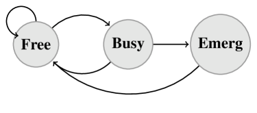
During online execution, robot i𝑖i tries to satisfy its specification safely by resolving conflicts with other robots. This is done by following some mode switching rules encoded into a finite state machine (FSM), see Fig. 2. Each FSM has the following three modes:

  • Free: Robot moves as planned. This is the normal mode.

  • Busy: Robot enters this mode when conflicts are detected. In this mode, the planning order assignment module and the trajectory planning module are activated.

  • Emerg: Robot starts an emergency stop process.
Refer to caption
Figure 2: The three modes of robot i𝑖i and the transitions among them.

In Fig. 2, the transitions between different modes of the FSM are depicted. Initially, robot i𝑖i is in Free mode. The conflict detection module is activated when the online execution starts. Once conflict neighbors (will be defined later) are detected, robot i𝑖i enters to Busy mode and the planning order assignment and the trajectory planning modules are activated to solve the conflicts, otherwise, robot i𝑖i stays in Free mode. When robot i𝑖i is in Busy mode, it switches back to Free mode if the trajectory planning module returns a feasible solution, and the solution will be broadcasted to the robot’s neighboring area as well as sent to the controller for execution, otherwise (e.g., no feasible plan is found), robot i𝑖i switches to Emerg mode and a braking controller (defined later) is applied. Note that when robot i𝑖i switches to Emerg mode, it will come to a stop but with power-on. This means that robot i𝑖i will continue monitoring the environment and restart (switches back to Free mode) when it is possible.

IV-B Offline pre-computation

IV-B1 Braking controller

As stated in the previous subsection, when robot i𝑖i enters Emerg mode, it starts an emergency stop process. In our previous work [21], safety in Emerg mode is guaranteed by assuming that each robot can take unbounded input when switching to Emerg mode. In this work, we consider bounded input in all modes for all robots. Due to this, a braking controller needs to be designed for each robot, and the notions of braking (position) trajectory and braking time and distance are introduced.

Given the initial state xi𝕏isubscript𝑥𝑖subscript𝕏𝑖x_{i}\in\mathbb{X}_{i} of robot i𝑖i, define

ti(xi):=minTassignsuperscriptsubscript𝑡𝑖subscript𝑥𝑖𝑇\displaystyle t_{i}^{*}(x_{i}):=\min\quad T (11a)
subject to
xi(0)=xi,subscript𝑥𝑖0subscript𝑥𝑖\displaystyle x_{i}(0)=x_{i}, (11b)
x˙i(t)=Fi(xi(t),ui(t)),subscript˙𝑥𝑖𝑡subscript𝐹𝑖subscript𝑥𝑖𝑡subscript𝑢𝑖𝑡\displaystyle{\dot{x}}_{i}(t)=F_{i}(x_{i}(t),u_{i}(t)), (11c)
xi(t)𝕏i,ui(t)𝕌i,t[0,T)formulae-sequencesubscript𝑥𝑖𝑡subscript𝕏𝑖formulae-sequencesubscript𝑢𝑖𝑡subscript𝕌𝑖𝑡0𝑇\displaystyle x_{i}(t)\in\mathbb{X}_{i},u_{i}(t)\in\mathbb{U}_{i},t\in[0,T) (11d)
p˙i(T)=0l,subscript˙𝑝𝑖𝑇subscript0𝑙\displaystyle\dot{p}_{i}(T)=0_{l}, (11e)

as the minimal time needed to decelerate robot i𝑖i to zero velocity (i.e., p˙i(t)=0lsubscript˙𝑝𝑖𝑡subscript0𝑙\dot{p}_{i}(t)=0_{l}). Let 𝒖i(xi)superscriptsubscript𝒖𝑖subscript𝑥𝑖{\bm{u}}_{i}^{*}(x_{i}) be the optimal solution of (11). Then, the braking controller 𝒖ibr(xi)superscriptsubscript𝒖𝑖brsubscript𝑥𝑖{\bm{u}}_{i}^{\text{br}}(x_{i}) is designed as

uibr(xi)(t)={ui(xi)(t),if p˙i(t)0l,0m,if p˙i(t)=0l.superscriptsubscript𝑢𝑖brsubscript𝑥𝑖𝑡casessuperscriptsubscript𝑢𝑖subscript𝑥𝑖𝑡if subscript˙𝑝𝑖𝑡subscript0𝑙subscript0𝑚if subscript˙𝑝𝑖𝑡subscript0𝑙u_{i}^{\text{br}}(x_{i})(t)=\begin{cases}{u}_{i}^{*}(x_{i})(t),&\mbox{if }\dot{p}_{i}(t)\neq 0_{l},\\ 0_{m},&\mbox{if }\dot{p}_{i}(t)=0_{l}.\end{cases} (12)

Denote by 𝝃ibr(xi)superscriptsubscript𝝃𝑖brsubscript𝑥𝑖{\bm{\xi}}_{i}^{\text{br}}(x_{i}) the braking trajectory of robot i𝑖i starting at xisubscript𝑥𝑖x_{i}. Then we have

ξibr(xi)(t)=ξi(xi,𝒖ibr(xi),t),t[0,ti(xi)].formulae-sequencesuperscriptsubscript𝜉𝑖brsubscript𝑥𝑖𝑡subscript𝜉𝑖subscript𝑥𝑖superscriptsubscript𝒖𝑖brsubscript𝑥𝑖𝑡𝑡0superscriptsubscript𝑡𝑖subscript𝑥𝑖\xi_{i}^{\text{br}}(x_{i})(t)=\xi_{i}(x_{i},{\bm{u}}_{i}^{\text{br}}(x_{i}),t),t\in[0,t_{i}^{*}(x_{i})]. (13)

The braking position trajectory of robot i𝑖i, denoted by 𝒑ibr(xi)superscriptsubscript𝒑𝑖brsubscript𝑥𝑖{\bm{p}}_{i}^{\text{br}}(x_{i}), is then given by

𝒑ibr(xi)=projl(𝝃ibr(xi)).superscriptsubscript𝒑𝑖brsubscript𝑥𝑖subscriptproj𝑙superscriptsubscript𝝃𝑖brsubscript𝑥𝑖\displaystyle{\bm{p}}_{i}^{\text{br}}(x_{i})=\texttt{proj}_{l}({\bm{\xi}}_{i}^{\text{br}}(x_{i})). (14)

Let di(xi):=maxp𝒑ibr(xi)pprojl(xi).assignsuperscriptsubscript𝑑𝑖subscript𝑥𝑖subscript𝑝superscriptsubscript𝒑𝑖brsubscript𝑥𝑖norm𝑝subscriptproj𝑙subscript𝑥𝑖d_{i}^{*}(x_{i}):=\max_{p\in{\bm{p}}_{i}^{\text{br}}(x_{i})}\|p-\texttt{proj}_{l}(x_{i})\|. Then, we have the following assumption.

Assumption 2

Define the braking time Tibrsuperscriptsubscript𝑇𝑖brT_{i}^{\text{br}} and the braking distance Dibrsuperscriptsubscript𝐷𝑖brD_{i}^{\text{br}} as

Tibrsuperscriptsubscript𝑇𝑖br\displaystyle T_{i}^{\text{br}} :=assign\displaystyle:= maxxi𝕏i{ti(xi)},subscriptsubscript𝑥𝑖subscript𝕏𝑖superscriptsubscript𝑡𝑖subscript𝑥𝑖\displaystyle\max_{x_{i}\in\mathbb{X}_{i}}\{t_{i}^{*}(x_{i})\}, (15)
Dibrsuperscriptsubscript𝐷𝑖br\displaystyle D_{i}^{\text{br}} :=assign\displaystyle:= maxxi𝕏i{di(xi)}.subscriptsubscript𝑥𝑖subscript𝕏𝑖superscriptsubscript𝑑𝑖subscript𝑥𝑖\displaystyle\max_{x_{i}\in\mathbb{X}_{i}}\{d_{i}^{*}(x_{i})\}. (16)

Then, we have 0Tibr<0superscriptsubscript𝑇𝑖br0\leq T_{i}^{\text{br}}<\infty and 0Dibr<,iformulae-sequence0superscriptsubscript𝐷𝑖brfor-all𝑖0\leq D_{i}^{\text{br}}<\infty,\forall i.

Remark 2

Assumption 2 means that for any given initial state xi𝕏isubscript𝑥𝑖subscript𝕏𝑖x_{i}\in\mathbb{X}_{i}, the maximal time and distance needed for braking with the braking controller (12) are finite. We note that this assumption is not conservative as it is satisfied by many real-life robots. For robots with first-order dynamics (e.g., omni-directional robots, differential drive robots), i.e., the velocity of the robot is controlled, one can derive that Tibr=0superscriptsubscript𝑇𝑖br0T_{i}^{\text{br}}=0 and Dibr=0superscriptsubscript𝐷𝑖br0D_{i}^{\text{br}}=0 with the braking controller 𝐮ibr0msuperscriptsubscript𝐮𝑖brsubscript0𝑚\bm{u}_{i}^{\text{br}}\equiv 0_{m}. For robots with second-order dynamics (e.g., automated vehicles), i.e., the acceleration of the robot is controlled, the braking time Tibrsuperscriptsubscript𝑇𝑖brT_{i}^{\text{br}} and the braking distance Tibrsuperscriptsubscript𝑇𝑖brT_{i}^{\text{br}} are usually determined by the maximum velocity and acceleration.

Example 1

Consider a homogeneous MRS, where the dynamics of each robot i𝑖i is given by

p˙xisuperscriptsubscript˙𝑝𝑥𝑖\displaystyle\dot{p}_{x}^{i} =vicosθi,absentsubscript𝑣𝑖subscript𝜃𝑖\displaystyle=v_{i}\cos\theta_{i}, (17)
p˙yisuperscriptsubscript˙𝑝𝑦𝑖\displaystyle\dot{p}_{y}^{i} =visinθi,absentsubscript𝑣𝑖subscript𝜃𝑖\displaystyle=v_{i}\sin\theta_{i},
θ˙isubscript˙𝜃𝑖\displaystyle\dot{\theta}_{i} =ωi,absentsubscript𝜔𝑖\displaystyle=\omega_{i},
v˙isubscript˙𝑣𝑖\displaystyle\dot{v}_{i} =ai,absentsubscript𝑎𝑖\displaystyle=a_{i},

where pi:=(pxi,pyi)2assignsubscript𝑝𝑖superscriptsubscript𝑝𝑥𝑖superscriptsubscript𝑝𝑦𝑖superscript2p_{i}:=(p_{x}^{i},p_{y}^{i})\in\mathbb{R}^{2} is the position of robot i𝑖i, ζi:=(θi,vi)assignsubscript𝜁𝑖subscript𝜃𝑖subscript𝑣𝑖\zeta_{i}:=(\theta_{i},v_{i}) represents the non-position state of robot i𝑖i, which contains its orientation θisubscript𝜃𝑖\theta_{i}\in\mathbb{R} and velocity visubscript𝑣𝑖v_{i}\in\mathbb{R}. The input uisubscript𝑢𝑖u_{i} is given by ui:=(ωi,ai)assignsubscript𝑢𝑖subscript𝜔𝑖subscript𝑎𝑖u_{i}:=(\omega_{i},a_{i}), where ωisubscript𝜔𝑖\omega_{i} is the turning rate and aisubscript𝑎𝑖a_{i} is the acceleration.

The velocity and input of robot i𝑖i are subject to the hard constraints

|vi(t)|vi,max,|ωi(t)|ωi,max,|ai(t)|ai,max,formulae-sequencesubscript𝑣𝑖𝑡subscript𝑣𝑖formulae-sequencesubscript𝜔𝑖𝑡subscript𝜔𝑖subscript𝑎𝑖𝑡subscript𝑎𝑖\displaystyle|v_{i}(t)|\leq v_{i,\max},|\omega_{i}(t)|\leq\omega_{i,\max},|a_{i}(t)|\leq a_{i,\max}, (18)

where vi,max,ωi,max,ai,max>0subscript𝑣𝑖subscript𝜔𝑖subscript𝑎𝑖0v_{i,\max},\omega_{i,\max},a_{i,\max}>0. Then, the state and input sets are given by

𝕏i:={(pi,θi,vi):pi𝕎,θi,|vi|vi,max},assignsubscript𝕏𝑖conditional-setsubscript𝑝𝑖subscript𝜃𝑖subscript𝑣𝑖formulae-sequencesubscript𝑝𝑖𝕎formulae-sequencesubscript𝜃𝑖subscript𝑣𝑖subscript𝑣𝑖\displaystyle\mathbb{X}_{i}:=\{(p_{i},\theta_{i},v_{i}):p_{i}\in\mathbb{W},\theta_{i}\in\mathbb{R},|v_{i}|\leq v_{i,\max}\}, (19)
𝕌i:={(ωi,ai):|ωi|ωi,max,|ai|ai,max}.assignsubscript𝕌𝑖conditional-setsubscript𝜔𝑖subscript𝑎𝑖formulae-sequencesubscript𝜔𝑖subscript𝜔𝑖subscript𝑎𝑖subscript𝑎𝑖\displaystyle\mathbb{U}_{i}:=\{(\omega_{i},a_{i}):|\omega_{i}|\leq\omega_{i,\max},|a_{i}|\leq a_{i,\max}\}. (20)

In this example, we consider two different braking controllers. First, design the braking controller 𝐮ibr, 1superscriptsubscript𝐮𝑖br, 1\bm{u}_{i}^{\text{br, 1}} as

uibr, 1(t)={(0,ai,maxvi(t)|vi(t)|),if|vi(t)|0,02,if|vi(t)|=0.u_{i}^{\text{br, 1}}(t)=\left\{\begin{aligned} \left(0,-a_{i,\max}\frac{v_{i}(t)}{|v_{i}(t)|}\right),&\quad\text{if}\;|v_{i}(t)|\neq 0,\\ 0_{2}\quad\quad\quad,&\quad\text{if}\;|v_{i}(t)|=0.\end{aligned}\right. (21)

Then, one can derive the braking time Tibr, 1=|vi,max|/ai,maxsuperscriptsubscript𝑇𝑖br, 1subscript𝑣𝑖subscript𝑎𝑖T_{i}^{\text{br, 1}}={|v_{i,\max}|}/{a_{i,\max}} and the braking distance Dibr, 1=|vi,max|2/2ai,maxsuperscriptsubscript𝐷𝑖br, 1superscriptsubscript𝑣𝑖22subscript𝑎𝑖D_{i}^{\text{br, 1}}=|v_{i,\max}|^{2}/2{a_{i,\max}}.

Alternatively, one can design the braking controller 𝐮ibr, 2superscriptsubscript𝐮𝑖br, 2\bm{u}_{i}^{\text{br, 2}} as

uibr, 2(t)={(()ωi,max,ai,maxvi(t)|vi(t)|),if|vi(t)|0,02,if|vi(t)|=0.u_{i}^{\text{br, 2}}(t)=\left\{\begin{aligned} \left((-)\omega_{i,\max},-a_{i,\max}\frac{v_{i}(t)}{|v_{i}(t)|}\right),&\quad\text{if}\;|v_{i}(t)|\neq 0,\\ 0_{2}\quad\quad\quad,&\quad\text{if}\;|v_{i}(t)|=0.\end{aligned}\right. (22)

Then, one can derive the braking time Tibr, 2=|vi,max|/ai,maxsuperscriptsubscript𝑇𝑖br, 2subscript𝑣𝑖subscript𝑎𝑖T_{i}^{\text{br, 2}}={|v_{i,\max}|}/{a_{i,\max}} and the braking distance

Dibr, 2=g(vi,max,ωi,max,ai,max)ωi,max2,superscriptsubscript𝐷𝑖br, 2𝑔subscript𝑣𝑖subscript𝜔𝑖subscript𝑎𝑖superscriptsubscript𝜔𝑖2D_{i}^{\text{br, 2}}=\frac{g(v_{i,\max},\omega_{i,\max},a_{i,\max})}{\omega_{i,\max}^{2}},

where g(vi,max,ωi,max,ai,max)=vi,max2ωi,max2+2ai,max2(1cos(vi,maxωi,max/ai,max))2vi,maxωi,maxai,maxsin(vi,maxωi,max/ai,max)𝑔subscript𝑣𝑖subscript𝜔𝑖subscript𝑎𝑖superscriptsubscript𝑣𝑖2superscriptsubscript𝜔𝑖22superscriptsubscript𝑎𝑖21subscript𝑣𝑖subscript𝜔𝑖subscript𝑎𝑖2subscript𝑣𝑖subscript𝜔𝑖subscript𝑎𝑖subscript𝑣𝑖subscript𝜔𝑖subscript𝑎𝑖g(v_{i,\max},\omega_{i,\max},a_{i,\max})=v_{i,\max}^{2}\omega_{i,\max}^{2}+2a_{i,\max}^{2}\Big{(}1-\cos({v_{i,\max}\omega_{i,\max}}/{a_{i,\max}})\Big{)}-2v_{i,\max}\omega_{i,\max}a_{i,\max}\sin{({v_{i,\max}\omega_{i,\max}}/{a_{i,\max}})}. Note that using the braking controller (22), one can prove that the minimal braking distance is achieved.

IV-B2 Workspace discretization

Given the set of AP𝐴𝑃AP, Assumption 1 guarantees that there exists an observation preserving cell decomposition Φ={X1,,XM}Φsubscript𝑋1subscript𝑋𝑀\Phi=\{X_{1},\ldots,X_{M}\} over the workspace 𝕎𝕎\mathbb{W}. In general, Xl1,Xl2,l1l2subscript𝑋subscript𝑙1subscript𝑋subscript𝑙2subscript𝑙1subscript𝑙2X_{l_{1}},X_{l_{2}},l_{1}\neq l_{2} are of different shapes and sizes. For the sake of online coordination, we propose to further discretize each cell XlΦsubscript𝑋𝑙ΦX_{l}\in\Phi into smaller regions. Let Ξ(Xl):={X^l1,,X^lMl}assignΞsubscript𝑋𝑙superscriptsubscript^𝑋𝑙1superscriptsubscript^𝑋𝑙subscript𝑀𝑙\Xi(X_{l}):=\{\hat{X}_{l}^{1},\ldots,\hat{X}_{l}^{M_{l}}\} be a partition of Xlsubscript𝑋𝑙X_{l} into Mlsubscript𝑀𝑙M_{l} disjoint convex regions. Then, we define Ξ:=XlΦΞ(Xl)assignΞsubscriptsubscript𝑋𝑙ΦΞsubscript𝑋𝑙\Xi:=\cup_{X_{l}\in\Phi}\Xi(X_{l}). ΞΞ\Xi can be seen as a finer discretization over the workspace 𝕎𝕎\mathbb{W}.

Given a set S𝕎𝑆𝕎S\subseteq\mathbb{W}, let

Q^(S):={X^Ξ:X^S},assign^𝑄𝑆conditional-set^𝑋Ξ^𝑋𝑆\hat{Q}(S):=\{\hat{X}\in\Xi:\hat{X}\cap S\neq\emptyset\}, (23)

which represents the set of regions in ΞΞ\Xi that intersect with S𝑆S.

IV-B3 Pre-computation of braking area, CTS, NBA, PBA, and potential functions

Given the position pisubscript𝑝𝑖p_{i} of robot i𝑖i, define

𝕊i(pi):={xi𝕏i:projl(xi)=pi}assignsubscript𝕊𝑖subscript𝑝𝑖conditional-setsubscript𝑥𝑖subscript𝕏𝑖subscriptproj𝑙subscript𝑥𝑖subscript𝑝𝑖\mathbb{S}_{i}(p_{i}):=\{x_{i}\in\mathbb{X}_{i}:\texttt{proj}_{l}(x_{i})=p_{i}\}

as the subset of states in 𝕏isubscript𝕏𝑖\mathbb{X}_{i} that correspond to pisubscript𝑝𝑖p_{i}. In addition, we define the braking area of robot i𝑖i at position pisubscript𝑝𝑖p_{i} as

Φ(pi):=xi𝕊i(pi)ϕi(𝒑ibr(xi)),assignΦsubscript𝑝𝑖subscriptsubscript𝑥𝑖subscript𝕊𝑖subscript𝑝𝑖subscriptitalic-ϕ𝑖superscriptsubscript𝒑𝑖brsubscript𝑥𝑖\Phi(p_{i}):=\cup_{x_{i}\in\mathbb{S}_{i}(p_{i})}\phi_{i}({\bm{p}}_{i}^{\text{br}}(x_{i})), (24)

where ϕi(𝒑ibr(xi))subscriptitalic-ϕ𝑖superscriptsubscript𝒑𝑖brsubscript𝑥𝑖\phi_{i}({\bm{p}}_{i}^{\text{br}}(x_{i})) is the footprint of the braking position trajectory 𝒑ibr(xi)superscriptsubscript𝒑𝑖brsubscript𝑥𝑖{\bm{p}}_{i}^{\text{br}}(x_{i}). Let

ψi(pi):=(ϕi(pi),Dibr).assignsubscript𝜓𝑖subscript𝑝𝑖subscriptitalic-ϕ𝑖subscript𝑝𝑖superscriptsubscript𝐷𝑖br\psi_{i}(p_{i}):=\mathcal{B}(\phi_{i}(p_{i}),D_{i}^{\text{br}}). (25)

Then, we have the following result.

Proposition 1

The braking area of robot i𝑖i at position pisubscript𝑝𝑖p_{i} can be over-approximated by the set ψi(pi)subscript𝜓𝑖subscript𝑝𝑖\psi_{i}(p_{i}), that is,

Φ(pi)(ϕi(pi),Dibr),pi𝕎.formulae-sequenceΦsubscript𝑝𝑖subscriptitalic-ϕ𝑖subscript𝑝𝑖superscriptsubscript𝐷𝑖brfor-allsubscript𝑝𝑖𝕎\Phi(p_{i})\subseteq\mathcal{B}(\phi_{i}(p_{i}),D_{i}^{\text{br}}),\forall p_{i}\in\mathbb{W}.

In addition, for each region X^lΞsubscript^𝑋𝑙Ξ\hat{X}_{l}\in\Xi, define

ψi(X^l):=assignsubscript𝜓𝑖subscript^𝑋𝑙absent\displaystyle\psi_{i}(\hat{X}_{l}):= piX^lψi(pi).subscriptsubscript𝑝𝑖subscript^𝑋𝑙subscript𝜓𝑖subscript𝑝𝑖\displaystyle\cup_{p_{i}\in\hat{X}_{l}}\psi_{i}(p_{i}). (26)

Each robot i𝑖i will compute offline a map Mi:Ξ2Ξ:subscript𝑀𝑖Ξsuperscript2ΞM_{i}:\Xi\to 2^{\Xi}, where

Mi(X^l):=Q^(ψi(X^l)),X^lΞ.formulae-sequenceassignsubscript𝑀𝑖subscript^𝑋𝑙^𝑄subscript𝜓𝑖subscript^𝑋𝑙for-allsubscript^𝑋𝑙Ξ\displaystyle M_{i}(\hat{X}_{l}):=\hat{Q}\left(\psi_{i}(\hat{X}_{l})\right),\forall\hat{X}_{l}\in\Xi. (27)

Intuitively, Misubscript𝑀𝑖M_{i} projects a region X^lsubscript^𝑋𝑙\hat{X}_{l} into a set of regions that might be traversed by the braking position trajectory of robot i𝑖i if robot i𝑖i starts an emergency stop process inside X^lsubscript^𝑋𝑙\hat{X}_{l}.

Due to the continuity of the dynamics, the state and the input spaces, the transition system that represents (7) is infinite for each robot i𝑖i. To this end, a probabilistically complete sampling-based algorithm is proposed in [25] to approximate (7) by a finite transition system. Given a sampling interval τssubscript𝜏𝑠\tau_{s}, the finite transition system that represents (7) is denoted by 𝒯i:=(𝕏^i,𝕏^i0,𝕌i,c,i,Fi,𝕎,h)assignsubscript𝒯𝑖subscript^𝕏𝑖superscriptsubscript^𝕏𝑖0subscript𝕌𝑖subscript𝑐𝑖subscript𝐹𝑖𝕎\mathcal{T}_{i}:=(\hat{\mathbb{X}}_{i},\hat{\mathbb{X}}_{i}^{0},\mathbb{U}_{i},\rightarrow_{c,i},F_{i},\mathbb{W},h), where

  • 𝕏^isubscript^𝕏𝑖\hat{\mathbb{X}}_{i} collects all sampling points in 𝕏isubscript𝕏𝑖\mathbb{X}_{i} that are safe (with respect to the static obstacles), i.e., ψi(projl(xi))𝔽,xi𝕏^iformulae-sequencesubscript𝜓𝑖subscriptproj𝑙subscript𝑥𝑖𝔽for-allsubscript𝑥𝑖subscript^𝕏𝑖\psi_{i}(\texttt{proj}_{l}(x_{i}))\subseteq\mathbb{F},\forall x_{i}\in\hat{\mathbb{X}}_{i}),

  • 𝕏^i0𝕏^isuperscriptsubscript^𝕏𝑖0subscript^𝕏𝑖\hat{\mathbb{X}}_{i}^{0}\subseteq\hat{\mathbb{X}}_{i},

  • c,i𝕏^i×𝕌i×𝕏^i\rightarrow_{c,i}\subseteq\hat{\mathbb{X}}_{i}\times\mathbb{U}_{i}\times\hat{\mathbb{X}}_{i},

Fisubscript𝐹𝑖F_{i} is given in (7), 𝕎𝕎\mathbb{W} is the workspace as well as the observation space, and h()=projl()subscriptproj𝑙h(\cdot)=\texttt{proj}_{l}(\cdot) is the observation map. Here, 𝕏i,𝕌isubscript𝕏𝑖subscript𝕌𝑖\mathbb{X}_{i},\mathbb{U}_{i} are the set of states and inputs, which are defined in (8). The transition relation (xi,ui,xi)c,isubscript𝑥𝑖subscript𝑢𝑖subscriptsuperscript𝑥𝑖subscript𝑐𝑖(x_{i},u_{i},x^{\prime}_{i})\in\rightarrow_{c,i} if and only if xi=ξi(xi,ui,τs)subscriptsuperscript𝑥𝑖subscript𝜉𝑖subscript𝑥𝑖subscript𝑢𝑖subscript𝜏𝑠x^{\prime}_{i}=\xi_{i}(x_{i},u_{i},\tau_{s}). Similarly to (4), define

Post(xi):={xi𝕏^i:ui𝕌i,xiuixi}.assign𝑃𝑜𝑠𝑡subscript𝑥𝑖conditional-setsubscriptsuperscript𝑥𝑖subscript^𝕏𝑖formulae-sequencesubscript𝑢𝑖subscript𝕌𝑖subscript𝑢𝑖subscript𝑥𝑖subscriptsuperscript𝑥𝑖Post(x_{i}):=\{x^{\prime}_{i}\in\hat{\mathbb{X}}_{i}:\exists u_{i}\in\mathbb{U}_{i},x_{i}\xrightarrow[]{u_{i}}x^{\prime}_{i}\}. (28)

Once 𝒯isubscript𝒯𝑖\mathcal{T}_{i} is obtained, one can further construct the NBA 𝖡i:=(Si,Si0,2APφi,δi,Fi)assignsubscript𝖡𝑖subscript𝑆𝑖superscriptsubscript𝑆𝑖0superscript2𝐴subscript𝑃subscript𝜑𝑖subscript𝛿𝑖subscript𝐹𝑖\mathsf{B}_{i}:=(S_{i},S_{i}^{0},2^{AP_{\varphi_{i}}},\delta_{i},F_{i}) for the specification φisubscript𝜑𝑖\varphi_{i} (Definition 1), the CTS 𝒯c,i:=(𝕏^i,𝕏^i0,APφi,c,i,Lc,i)assignsubscript𝒯𝑐𝑖subscript^𝕏𝑖superscriptsubscript^𝕏𝑖0𝐴subscript𝑃subscript𝜑𝑖subscript𝑐𝑖subscript𝐿𝑐𝑖\mathcal{T}_{c,i}:=(\hat{\mathbb{X}}_{i},\hat{\mathbb{X}}_{i}^{0},AP_{\varphi_{i}},\rightarrow_{c,i},L_{c,i}) (Definition 2), and then form the PBA 𝒫i=𝒯c,i×𝖡isubscript𝒫𝑖subscript𝒯𝑐𝑖subscript𝖡𝑖\mathcal{P}_{i}=\mathcal{T}_{c,i}\times\mathsf{B}_{i} (Definition 3). After that, the potential function for 𝒫isubscript𝒫𝑖\mathcal{P}_{i} can be computed according to Definition 6.

Remark 3

The cell decomposition ΦΦ\Phi of the workspace satisfies Lc(x)=Lc(x),Q(x)=Q(x)formulae-sequencesubscript𝐿𝑐𝑥subscript𝐿𝑐superscript𝑥for-all𝑄𝑥𝑄superscript𝑥L_{c}(x)=L_{c}(x^{\prime}),\forall Q(x)=Q(x^{\prime}). In addition, APφiAP,i𝒱formulae-sequence𝐴subscript𝑃subscript𝜑𝑖𝐴𝑃for-all𝑖𝒱AP_{\varphi_{i}}\subseteq AP,\forall i\in\mathcal{V}. Therefore, one has Lc,i(x)=Lc,i(x),Q(x)=Q(x),i𝒱formulae-sequencesubscript𝐿𝑐𝑖𝑥subscript𝐿𝑐𝑖superscript𝑥formulae-sequencefor-all𝑄𝑥𝑄superscript𝑥for-all𝑖𝒱L_{c,i}(x)=L_{c,i}(x^{\prime}),\forall Q(x)=Q(x^{\prime}),\forall i\in\mathcal{V} and thus β𝒫i(x)=β𝒫i(x),Q(x)=Q(x),i𝒱formulae-sequencesubscript𝛽subscript𝒫𝑖𝑥subscript𝛽subscript𝒫𝑖superscript𝑥formulae-sequencefor-all𝑄𝑥𝑄superscript𝑥for-all𝑖𝒱\beta_{\mathcal{P}_{i}}(x)=\beta_{\mathcal{P}_{i}}(x^{\prime}),\forall Q(x)=Q(x^{\prime}),\forall i\in\mathcal{V}. Then, according to Definition 6, one can get that if V𝒫i((x,β𝒫i(x)))<subscript𝑉subscript𝒫𝑖𝑥subscript𝛽subscript𝒫𝑖𝑥V_{\mathcal{P}_{i}}((x,\beta_{\mathcal{P}_{i}}(x)))<\infty, then V𝒫i((x,β𝒫i(x)))<,xQ(x)formulae-sequencesubscript𝑉subscript𝒫𝑖superscript𝑥subscript𝛽subscript𝒫𝑖superscript𝑥for-allsuperscript𝑥𝑄𝑥V_{\mathcal{P}_{i}}((x^{\prime},\beta_{\mathcal{P}_{i}}(x^{\prime})))<\infty,\forall x^{\prime}\in Q(x).

IV-C Initialization

Before proceeding, the following definition is required.

Definition 8

We call a trajectory 𝛏isubscript𝛏𝑖{\bm{\xi}}_{i} of (7) safely satisfy an LTL formula φisubscript𝜑𝑖\varphi_{i} if i) 𝛏iφimodelssubscript𝛏𝑖subscript𝜑𝑖{\bm{\xi}}_{i}\models\varphi_{i} and ii) ψi(pi)𝔽,piprojl(𝛏i)formulae-sequencesubscript𝜓𝑖subscript𝑝𝑖𝔽for-allsubscript𝑝𝑖subscriptproj𝑙subscript𝛏𝑖\psi_{i}(p_{i})\subseteq\mathbb{F},\forall{p}_{i}\in\texttt{proj}_{l}({\bm{\xi}}_{i}).

At the task activation time t=0𝑡0t=0, robot i𝑖i first finds a trajectory 𝝃i0superscriptsubscript𝝃𝑖0{\bm{\xi}}_{i}^{0} that safely satisfy φisubscript𝜑𝑖\varphi_{i}. The trajectory planning problem for a single robot can be solved by many existing methods, such as search- or sampling-based [28, 29], automata-based [30], and optimization-based methods [31, 32]. We note that the initial trajectory planning is not the focus of this paper. For details about this process, we refer to interested readers to corresponding literatures and the references therein.

The following assumption is needed to guarantee the feasibility of each task specification φisubscript𝜑𝑖\varphi_{i}.

Assumption 3

Initially, for each robot i𝑖i, there exists a trajectory 𝛏i0superscriptsubscript𝛏𝑖0{\bm{\xi}}_{i}^{0} that safely satisfy φisubscript𝜑𝑖\varphi_{i}.

IV-D Online motion coordination

The initially planned trajectory of each robot does not consider the motion of other robots. Moreover, each robot has only local view and local information (about other robots). Therefore, motion coordination is required during online implementation. Based on the sensing information (about the workspace) and broadcasted information (from neighboring robots), each robot can detect conflicts within its neighborhood and then conduct motion replanning such that conflicts are avoided. In this work, we consider that the conflict detection is conducted at a sequence of sampling instants {tk}ksubscriptsubscript𝑡𝑘𝑘\{t_{k}\}_{k\in\mathbb{N}} for each robot i𝑖i, where tk+1tkΔsubscript𝑡𝑘1subscript𝑡𝑘Δt_{k+1}-t_{k}\equiv\Delta.

IV-D1 Conflict detection

Before proceeding, the following notation is introduced. Given a position trajectory 𝒑i([t1,t2])subscript𝒑𝑖subscript𝑡1subscript𝑡2{\bm{p}}_{i}([t_{1},t_{2}]) and a region X^lΞsubscript^𝑋𝑙Ξ\hat{X}_{l}\in\Xi, the function Γ:(0,p)×Ξ20:Γsubscriptabsent0superscript𝑝Ξsuperscript2subscriptabsent0\Gamma:\mathcal{F}(\mathbb{R}_{\geq 0},\mathbb{R}^{p})\times\Xi\to 2^{\mathbb{R}_{\geq 0}}, defined as

Γ(𝒑i([t1,t2]),X^l):={t[t1,t2]:pi(t)X^l},assignΓsubscript𝒑𝑖subscript𝑡1subscript𝑡2subscript^𝑋𝑙conditional-set𝑡subscript𝑡1subscript𝑡2subscript𝑝𝑖𝑡subscript^𝑋𝑙\Gamma({\bm{p}}_{i}([t_{1},t_{2}]),\hat{X}_{l}):=\{t\in[t_{1},t_{2}]:p_{i}(t)\in\hat{X}_{l}\}, (29)

gives the time interval that the position trajectory pi([t1,t2])subscript𝑝𝑖subscript𝑡1subscript𝑡2p_{i}([t_{1},t_{2}]) occupies the region X^lsubscript^𝑋𝑙\hat{X}_{l}.

Given the position pi(tk)subscript𝑝𝑖subscript𝑡𝑘p_{i}(t_{k}), (pi(tk),R)subscript𝑝𝑖subscript𝑡𝑘𝑅\mathcal{B}(p_{i}(t_{k}),R) represents the sensing area of robot i𝑖i at time tksubscript𝑡𝑘t_{k} and Q^((pi(tk),R))^𝑄subscript𝑝𝑖subscript𝑡𝑘𝑅\hat{Q}(\mathcal{B}(p_{i}(t_{k}),R)) represents the set of regions in ΞΞ\Xi that intersect with (pi(tk),R)subscript𝑝𝑖subscript𝑡𝑘𝑅\mathcal{B}(p_{i}(t_{k}),R). Let

tifl(tk):=mint>tk{pi(t)(pi(tk),R)}assignsuperscriptsubscript𝑡𝑖𝑓𝑙subscript𝑡𝑘subscript𝑡subscript𝑡𝑘subscript𝑝𝑖𝑡subscript𝑝𝑖subscript𝑡𝑘𝑅t_{i}^{fl}(t_{k}):=\min_{t>t_{k}}\{p_{i}(t)\notin\mathcal{B}(p_{i}(t_{k}),R)\}

be the first time that robot i𝑖i leaves its sensing area (pi(tk),R)subscript𝑝𝑖subscript𝑡𝑘𝑅\mathcal{B}(p_{i}(t_{k}),R). Then, define

Si(tk):=Q^(𝒑i([tk,tifl(tk)]))assignsubscript𝑆𝑖subscript𝑡𝑘^𝑄subscript𝒑𝑖subscript𝑡𝑘superscriptsubscript𝑡𝑖𝑓𝑙subscript𝑡𝑘S_{i}(t_{k}):=\hat{Q}\big{(}{\bm{p}}_{i}([t_{k},t_{i}^{fl}(t_{k})])\big{)} (30)

as the set of regions traversed by robot i𝑖i within (pi(tk),R)subscript𝑝𝑖subscript𝑡𝑘𝑅\mathcal{B}(p_{i}(t_{k}),R) until it leaves it at tifl(tk)superscriptsubscript𝑡𝑖𝑓𝑙subscript𝑡𝑘t_{i}^{fl}(t_{k}). Moreover, for each X^lSi(tk)subscript^𝑋𝑙subscript𝑆𝑖subscript𝑡𝑘\hat{X}_{l}\in S_{i}(t_{k}), the braking area of robot i𝑖i is contained in ψi(X^l)subscript𝜓𝑖subscript^𝑋𝑙\psi_{i}(\hat{X}_{l}). Then, we define

Resi(X^l):=Mi(X^l)assign𝑅𝑒subscript𝑠𝑖subscript^𝑋𝑙subscript𝑀𝑖subscript^𝑋𝑙Res_{i}(\hat{X}_{l}):=M_{i}(\hat{X}_{l}) (31)

as the set of reserved regions by robot i𝑖i in order to safely brake when robot i𝑖i is within X^lsubscript^𝑋𝑙\hat{X}_{l}. According to (29), the time interval that robot i𝑖i occupies the region X^lSi(tk)subscript^𝑋𝑙subscript𝑆𝑖subscript𝑡𝑘\hat{X}_{l}\in S_{i}(t_{k}) is given by Γ(𝒑i([tk,tifl(tk)]),X^l)Γsubscript𝒑𝑖subscript𝑡𝑘superscriptsubscript𝑡𝑖𝑓𝑙subscript𝑡𝑘subscript^𝑋𝑙\Gamma({\bm{p}}_{i}([t_{k},t_{i}^{fl}(t_{k})]),{\hat{X}}_{l}). In addition, by the continuity of 𝒑i([tk,))subscript𝒑𝑖subscript𝑡𝑘{\bm{p}}_{i}([t_{k},\infty)), one can conclude that Γ(𝒑i([tk,tifl(tk)]),X^l)Γsubscript𝒑𝑖subscript𝑡𝑘superscriptsubscript𝑡𝑖𝑓𝑙subscript𝑡𝑘subscript^𝑋𝑙\Gamma({\bm{p}}_{i}([t_{k},t_{i}^{fl}(t_{k})]),{\hat{X}}_{l}) is given by one or several disjoint time interval(s) of the form [a,b),a<b𝑎𝑏𝑎𝑏[a,b),a<b. Supposing that

Γ(𝒑i([tk,tifl(tk)]),X^l)=l=1m[al,bl),Γsubscript𝒑𝑖subscript𝑡𝑘superscriptsubscript𝑡𝑖𝑓𝑙subscript𝑡𝑘subscript^𝑋𝑙superscriptsubscript𝑙1𝑚subscript𝑎𝑙subscript𝑏𝑙\Gamma({\bm{p}}_{i}([t_{k},t_{i}^{fl}(t_{k})]),{\hat{X}}_{l})=\cup_{l=1}^{m}[a_{l},b_{l}), (32)

where m𝑚m is the number of disjoint intervals in Γ(𝒑i([tk,tifl(tk)]),X^l)Γsubscript𝒑𝑖subscript𝑡𝑘superscriptsubscript𝑡𝑖𝑓𝑙subscript𝑡𝑘subscript^𝑋𝑙\Gamma({\bm{p}}_{i}([t_{k},t_{i}^{fl}(t_{k})]),{\hat{X}}_{l}). Denote by 𝒯i(X^l)subscript𝒯𝑖subscript^𝑋𝑙\mathcal{T}_{i}(\hat{X}_{l}) the time interval that robot i𝑖i reserves the area Resi(X^l)𝑅𝑒subscript𝑠𝑖subscript^𝑋𝑙Res_{i}(\hat{X}_{l}). Then, it can be over-approximated by

𝒯i(X^l):=l=1m[al,bl+Tibr),assignsubscript𝒯𝑖subscript^𝑋𝑙superscriptsubscript𝑙1𝑚subscript𝑎𝑙subscript𝑏𝑙superscriptsubscript𝑇𝑖br\mathcal{T}_{i}(\hat{X}_{l}):=\cup_{l=1}^{m}[a_{l},b_{l}+T_{i}^{\text{br}}), (33)

where Tibrsuperscriptsubscript𝑇𝑖brT_{i}^{\text{br}} is defined in (15). Then, we have the following definitions.

Definition 9

We say that there is a spatial-temporal conflict between robot i𝑖i and j𝑗j at time tksubscript𝑡𝑘t_{k} if X^lSi(tk),X^lSj(tk)formulae-sequencesubscript^𝑋𝑙subscript𝑆𝑖subscript𝑡𝑘subscript^𝑋superscript𝑙subscript𝑆𝑗subscript𝑡𝑘\exists\hat{X}_{l}\in S_{i}(t_{k}),\hat{X}_{l^{\prime}}\in S_{j}(t_{k}) such that Resi(X^l)Resj(X^l)𝑅𝑒subscript𝑠𝑖subscript^𝑋𝑙𝑅𝑒subscript𝑠𝑗subscript^𝑋superscript𝑙Res_{i}(\hat{X}_{l})\cap Res_{j}(\hat{X}_{l^{\prime}})\neq\emptyset and 𝒯i(X^l)𝒯j(X^l)subscript𝒯𝑖subscript^𝑋𝑙subscript𝒯𝑗subscript^𝑋superscript𝑙\mathcal{T}_{i}(\hat{X}_{l})\cap\mathcal{T}_{j}(\hat{X}_{l^{\prime}})\neq\emptyset.

Based on Definition 9, we define the set of conflict neighbors of robot i𝑖i at time tksubscript𝑡𝑘t_{k}, denoted by 𝒩~i(tk)subscript~𝒩𝑖subscript𝑡𝑘\tilde{\mathcal{N}}_{i}(t_{k}), as

𝒩~isubscript~𝒩𝑖\displaystyle\tilde{\mathcal{N}}_{i} (tk):={j𝒩i(tk):X^lSi(tk),X^lSj(tk)s.t.\displaystyle(t_{k}):=\{j\in\mathcal{N}_{i}(t_{k}):\exists\hat{X}_{l}\in S_{i}(t_{k}),\hat{X}_{l^{\prime}}\in S_{j}(t_{k})\;\text{s.t.}\; (34)
Resi(X^l)Resj(X^l)𝒯i(X^l)𝒯j(X^l)}.\displaystyle Res_{i}(\hat{X}_{l})\cap Res_{j}(\hat{X}_{l^{\prime}})\neq\emptyset\wedge\mathcal{T}_{i}(\hat{X}_{l})\cap\mathcal{T}_{j}(\hat{X}_{l^{\prime}})\neq\emptyset\}.

Then, we have the following Proposition.

Proposition 2

For robot i𝑖i, if 𝒩~i(tk)=subscript~𝒩𝑖subscript𝑡𝑘\tilde{\mathcal{N}}_{i}(t_{k})=\emptyset, then one has

  • i)

    ψi(pi(t))ψj(pj(t))=,j𝒩i(tk),t[tk,tifl(tk)]formulae-sequencesubscript𝜓𝑖subscript𝑝𝑖𝑡subscript𝜓𝑗subscript𝑝𝑗𝑡formulae-sequencefor-all𝑗subscript𝒩𝑖subscript𝑡𝑘for-all𝑡subscript𝑡𝑘superscriptsubscript𝑡𝑖𝑓𝑙subscript𝑡𝑘\psi_{i}(p_{i}(t))\cap\psi_{j}(p_{j}(t))=\emptyset,\forall j\in\mathcal{N}_{i}(t_{k}),\forall t\in[t_{k},t_{i}^{fl}(t_{k})];

  • ii)

    ϕi(pi(t))ϕj(pj(t))=,j𝒩i(tk),t[tk,tifl(tk)]formulae-sequencesubscriptitalic-ϕ𝑖subscript𝑝𝑖𝑡subscriptitalic-ϕ𝑗subscript𝑝𝑗𝑡formulae-sequencefor-all𝑗subscript𝒩𝑖subscript𝑡𝑘for-all𝑡subscript𝑡𝑘superscriptsubscript𝑡𝑖𝑓𝑙subscript𝑡𝑘\phi_{i}(p_{i}(t))\cap\phi_{j}(p_{j}(t))=\emptyset,\forall j\in\mathcal{N}_{i}(t_{k}),\forall t\in[t_{k},t_{i}^{fl}(t_{k})].

Proof: Since Tibrsuperscriptsubscript𝑇𝑖brT_{i}^{\text{br}} is the maximum time required to decelerate robot i𝑖i to zero velocity under the braking controller (12), one has that Γ(𝒑ibr(pi(t)),X^l)𝒯i(X^l),t[tk,tifl(tk)]formulae-sequenceΓsuperscriptsubscript𝒑𝑖brsubscript𝑝𝑖𝑡subscript^𝑋𝑙subscript𝒯𝑖subscript^𝑋𝑙for-all𝑡subscript𝑡𝑘superscriptsubscript𝑡𝑖𝑓𝑙subscript𝑡𝑘\Gamma({\bm{p}}_{i}^{\text{br}}(p_{i}(t)),{\hat{X}}_{l})\subseteq\mathcal{T}_{i}(\hat{X}_{l}),\forall t\in[t_{k},t_{i}^{fl}(t_{k})]. In addition, according to (26), (27), and (31), one has that ψi(pi(t))Resi(X^l),pi(t)X^lformulae-sequencesubscript𝜓𝑖subscript𝑝𝑖𝑡𝑅𝑒subscript𝑠𝑖subscript^𝑋𝑙for-allsubscript𝑝𝑖𝑡subscript^𝑋𝑙\psi_{i}(p_{i}(t))\subseteq Res_{i}(\hat{X}_{l}),\forall p_{i}(t)\in\hat{X}_{l}. That is to say, 𝒩~i(tk)=subscript~𝒩𝑖subscript𝑡𝑘\tilde{\mathcal{N}}_{i}(t_{k})=\emptyset implies i).

For each region X^lΞsubscript^𝑋𝑙Ξ\hat{X}_{l}\in\Xi, define

ϕi(X^l):=piX^lϕi(pi).assignsubscriptitalic-ϕ𝑖subscript^𝑋𝑙subscriptsubscript𝑝𝑖subscript^𝑋𝑙subscriptitalic-ϕ𝑖subscript𝑝𝑖\phi_{i}(\hat{X}_{l}):=\cup_{p_{i}\in\hat{X}_{l}}\phi_{i}(p_{i}).

Then, one has ϕi(X^l)ψi(X^l)subscriptitalic-ϕ𝑖subscript^𝑋𝑙subscript𝜓𝑖subscript^𝑋𝑙\phi_{i}(\hat{X}_{l})\subseteq\psi_{i}(\hat{X}_{l}). The time interval that the footprint of robot i𝑖i occupies X^lsubscript^𝑋𝑙\hat{X}_{l} is given by Γ(𝒑i([t,tifl(tk)]),X^l)Γsubscript𝒑𝑖𝑡superscriptsubscript𝑡𝑖𝑓𝑙subscript𝑡𝑘subscript^𝑋𝑙\Gamma({\bm{p}}_{i}([t,t_{i}^{fl}(t_{k})]),{\hat{X}}_{l}) and Γ(𝒑i([t,tifl(tk)]),X^l)𝒯i(X^l)Γsubscript𝒑𝑖𝑡superscriptsubscript𝑡𝑖𝑓𝑙subscript𝑡𝑘subscript^𝑋𝑙subscript𝒯𝑖subscript^𝑋𝑙\Gamma({\bm{p}}_{i}([t,t_{i}^{fl}(t_{k})]),{\hat{X}}_{l})\subseteq\mathcal{T}_{i}(\hat{X}_{l}). Thus, one can further get that i) implies ii). \square

Robot i𝑖i switches to Busy mode if and only if the set of conflict neighbors is non-empty (i.e., 𝒩~i(tk)subscript~𝒩𝑖subscript𝑡𝑘\tilde{\mathcal{N}}_{i}(t_{k})\neq\emptyset). The conflict detection process is outlined in Algorithm 1.

Algorithm 1 conflictDetection
1:Sj(tk),Γ(𝒑j([tk,tjfl(tk)]),X^l),X^lSj(tk)subscript𝑆𝑗subscript𝑡𝑘Γsubscript𝒑𝑗subscript𝑡𝑘superscriptsubscript𝑡𝑗𝑓𝑙subscript𝑡𝑘subscript^𝑋𝑙for-allsubscript^𝑋𝑙subscript𝑆𝑗subscript𝑡𝑘S_{j}(t_{k}),\Gamma({\bm{p}}_{j}([t_{k},t_{j}^{fl}(t_{k})]),{\hat{X}}_{l}),\forall\hat{X}_{l}\in S_{j}(t_{k}) for each j𝒩i+(tk)𝑗superscriptsubscript𝒩𝑖subscript𝑡𝑘j\in\mathcal{N}_{i}^{+}(t_{k}).
2:Set of conflict neighbors 𝒩~i(tk)subscript~𝒩𝑖subscript𝑡𝑘\tilde{\mathcal{N}}_{i}(t_{k}).
3:Initialize 𝒩~i(tk)=subscript~𝒩𝑖subscript𝑡𝑘\tilde{\mathcal{N}}_{i}(t_{k})=\emptyset.
4:Compute Resj(X^l),𝒯j(X^l)𝑅𝑒subscript𝑠𝑗subscript^𝑋𝑙subscript𝒯𝑗subscript^𝑋𝑙Res_{j}(\hat{X}_{l}),\mathcal{T}_{j}(\hat{X}_{l}) for each j𝒩i+(tk),X^lSj(tk)formulae-sequence𝑗superscriptsubscript𝒩𝑖subscript𝑡𝑘subscript^𝑋𝑙subscript𝑆𝑗subscript𝑡𝑘j\in\mathcal{N}_{i}^{+}(t_{k}),\hat{X}_{l}\in S_{j}(t_{k}),
5:for j𝒩i(tk)𝑗subscript𝒩𝑖subscript𝑡𝑘j\in\mathcal{N}_{i}(t_{k}) do
6:     if X^lSi(tk),X^lSj(tk)formulae-sequencesubscript^𝑋𝑙subscript𝑆𝑖subscript𝑡𝑘subscript^𝑋superscript𝑙subscript𝑆𝑗subscript𝑡𝑘\exists\hat{X}_{l}\in S_{i}(t_{k}),\hat{X}_{l^{\prime}}\in S_{j}(t_{k}) s.t. Resi(X^l)Resj(X^l)𝒯i(X^l)𝒯i(X^l)𝑅𝑒subscript𝑠𝑖subscript^𝑋𝑙𝑅𝑒subscript𝑠𝑗subscript^𝑋superscript𝑙subscript𝒯𝑖subscript^𝑋𝑙subscript𝒯𝑖subscript^𝑋superscript𝑙Res_{i}(\hat{X}_{l})\cap Res_{j}(\hat{X}_{l^{\prime}})\neq\emptyset\wedge\mathcal{T}_{i}(\hat{X}_{l})\cap\mathcal{T}_{i}(\hat{X}_{l^{\prime}})\neq\emptyset then
7:         𝒩~i(tk)=𝒩~i(tk){j}subscript~𝒩𝑖subscript𝑡𝑘subscript~𝒩𝑖subscript𝑡𝑘𝑗\tilde{\mathcal{N}}_{i}(t_{k})=\tilde{\mathcal{N}}_{i}(t_{k})\cup\{j\},
8:     end if
9:end for
Remark 4

To implement Algorithm 1, each robot i𝑖i needs only to broadcast to its neighboring area local information about its plan. To be more specific, which region (e.g., X^lsubscript^𝑋𝑙\hat{X}_{l}) within the sensing area (pi(tk),R)subscript𝑝𝑖subscript𝑡𝑘𝑅\mathcal{B}(p_{i}(t_{k}),R) is occupied by robot i𝑖i and when that happens (i.e., Γ(𝐩i([t,tifl(tk)]),X^l)Γsubscript𝐩𝑖𝑡superscriptsubscript𝑡𝑖𝑓𝑙subscript𝑡𝑘subscript^𝑋𝑙\Gamma({\bm{p}}_{i}([t,t_{i}^{fl}(t_{k})]),{\hat{X}}_{l})). Note that the non-position information (i.e., ζi(t)subscript𝜁𝑖𝑡\zeta_{i}(t)) of each robot is not required to be broadcasted to the neighbors.

IV-D2 Determine planning order

Based on the neighboring relation and conflict relation, the graph 𝒢(tk)={𝒱,(tk)}𝒢subscript𝑡𝑘𝒱subscript𝑡𝑘\mathcal{G}(t_{k})=\{\mathcal{V},\mathcal{E}(t_{k})\} formed by the group of robots is naturally divided into one or multiple connected subgraphs, and the motion planning is conducted in parallel within each subgraph in a sequential manner. In order to do that, a planning order needs to be decided for each connected subgraph. In this work, we propose a simple rule to assign priorities between each pair of neighbors.

The number of neighbors and conflict neighbors of robot i𝑖i at time tksubscript𝑡𝑘t_{k} are given by |𝒩i(tk)|subscript𝒩𝑖subscript𝑡𝑘|\mathcal{N}_{i}(t_{k})| and |𝒩~i(tk)|subscript~𝒩𝑖subscript𝑡𝑘|\tilde{\mathcal{N}}_{i}(t_{k})|, respectively. Then, we have the following definition.

Definition 10

We say that robot i𝑖i has advantage over robot j𝑗j at time tksubscript𝑡𝑘t_{k} if 𝒩~j(tk)subscript~𝒩𝑗subscript𝑡𝑘\tilde{\mathcal{N}}_{j}(t_{k})\neq\emptyset and

1) |𝒩i(tk)|>|𝒩j(tk)|subscript𝒩𝑖subscript𝑡𝑘subscript𝒩𝑗subscript𝑡𝑘|\mathcal{N}_{i}(t_{k})|>|\mathcal{N}_{j}(t_{k})|; OR

2) |𝒩i(tk)|=|𝒩j(tk)|subscript𝒩𝑖subscript𝑡𝑘subscript𝒩𝑗subscript𝑡𝑘|\mathcal{N}_{i}(t_{k})|=|\mathcal{N}_{j}(t_{k})| and |𝒩~i(tk)|>|𝒩~j(tk)|subscript~𝒩𝑖subscript𝑡𝑘subscript~𝒩𝑗subscript𝑡𝑘|\tilde{\mathcal{N}}_{i}(t_{k})|>|\tilde{\mathcal{N}}_{j}(t_{k})|.

Let 𝒴i(tk)subscript𝒴𝑖subscript𝑡𝑘\mathcal{Y}_{i}(t_{k}) be the set of neighbors that have higher priority than robot i𝑖i at time tksubscript𝑡𝑘t_{k}. The planning order assignment process is outlined in Algorithm 2.

For each neighbor j𝒩i(tk)𝑗subscript𝒩𝑖subscript𝑡𝑘j\in\mathcal{N}_{i}(t_{k}), if j𝑗j is in Emerg mode (and thus will be viewed as a static obstacle) or 𝒩~j(tk)=subscript~𝒩𝑗subscript𝑡𝑘\tilde{\mathcal{N}}_{j}(t_{k})=\emptyset, then robot j𝑗j has higher priority (lines 3-5). Otherwise, robot j𝑗j has higher priority in motion planning if robot j𝑗j has advantage over robot i𝑖i (lines 6-8). However, for the special case, i.e., |𝒩i(tk)|=|𝒩j(tk)|subscript𝒩𝑖subscript𝑡𝑘subscript𝒩𝑗subscript𝑡𝑘|\mathcal{N}_{i}(t_{k})|=|\mathcal{N}_{j}(t_{k})| and |𝒩~i(tk)|=|𝒩~j(tk)|subscript~𝒩𝑖subscript𝑡𝑘subscript~𝒩𝑗subscript𝑡𝑘|\tilde{\mathcal{N}}_{i}(t_{k})|=|\tilde{\mathcal{N}}_{j}(t_{k})|, neither robot i𝑖i nor j𝑗j has advantage over the other. In this case, the priority is determined by the initially uniquely assigned priority score for each robot i𝑖i (i.e., Pi0Pj0,i,jsuperscriptsubscript𝑃𝑖0superscriptsubscript𝑃𝑗0for-all𝑖𝑗P_{i}^{0}\neq P_{j}^{0},\forall i,j). Denote by Pi0superscriptsubscript𝑃𝑖0P_{i}^{0} the priority score of robot i𝑖i. We say that robot i𝑖i has priority over j𝑗j if Pi0>Pj0superscriptsubscript𝑃𝑖0superscriptsubscript𝑃𝑗0P_{i}^{0}>P_{j}^{0} (lines 9-11).

Algorithm 2 planningOrderAssignment
1:𝒩j(tk),𝒩~j(tk),Pj0,j𝒩i(tk){i}subscript𝒩𝑗subscript𝑡𝑘subscript~𝒩𝑗subscript𝑡𝑘superscriptsubscript𝑃𝑗0𝑗subscript𝒩𝑖subscript𝑡𝑘𝑖\mathcal{N}_{j}(t_{k}),\tilde{\mathcal{N}}_{j}(t_{k}),P_{j}^{0},j\in\mathcal{N}_{i}(t_{k})\cup\{i\}.
2:Set of higher priority neighbors 𝒴i(tk)subscript𝒴𝑖subscript𝑡𝑘\mathcal{Y}_{i}(t_{k}).
3:Initialize 𝒴i(tk)=subscript𝒴𝑖subscript𝑡𝑘\mathcal{Y}_{i}(t_{k})=\emptyset.
4:for j𝒩i(tk)𝑗subscript𝒩𝑖subscript𝑡𝑘j\in\mathcal{N}_{i}(t_{k}) do,
5:     if j𝑗j is in Emerg mode or 𝒩~j(tk)=subscript~𝒩𝑗subscript𝑡𝑘\tilde{\mathcal{N}}_{j}(t_{k})=\emptyset then,
6:         𝒴i(tk)=𝒴i(tk)jsubscript𝒴𝑖subscript𝑡𝑘subscript𝒴𝑖subscript𝑡𝑘𝑗\mathcal{Y}_{i}(t_{k})=\mathcal{Y}_{i}(t_{k})\cup j,
7:     else
8:         if j𝑗j has advantage over i𝑖i then,
9:              𝒴i(tk)=𝒴i(tk)jsubscript𝒴𝑖subscript𝑡𝑘subscript𝒴𝑖subscript𝑡𝑘𝑗\mathcal{Y}_{i}(t_{k})=\mathcal{Y}_{i}(t_{k})\cup j,
10:         else
11:              if neither robot i𝑖i nor j𝑗j has advantage over the other and Pj0>Pi0superscriptsubscript𝑃𝑗0superscriptsubscript𝑃𝑖0P_{j}^{0}>P_{i}^{0} then,
12:                  𝒴i(tk)=𝒴i(tk)jsubscript𝒴𝑖subscript𝑡𝑘subscript𝒴𝑖subscript𝑡𝑘𝑗\mathcal{Y}_{i}(t_{k})=\mathcal{Y}_{i}(t_{k})\cup j,
13:              end if
14:         end if
15:     end if
16:end for
Proposition 3 (Deadlock-free in planning order assignment)

The planning order assignment rule given in Algorithm 2 will result in no cycles, i.e., {qm}1K^,K^2\nexists\{q_{m}\}_{1}^{\hat{K}},{\hat{K}}\geq 2 such that qK^𝒴q1(tk)subscript𝑞^𝐾subscript𝒴subscript𝑞1subscript𝑡𝑘q_{\hat{K}}\in\mathcal{Y}_{q_{1}}(t_{k}) and qm1𝒴qm(tk),m=2,,K^formulae-sequencesubscript𝑞𝑚1subscript𝒴subscript𝑞𝑚subscript𝑡𝑘for-all𝑚2^𝐾q_{m-1}\in\mathcal{Y}_{q_{m}}(t_{k}),\forall m=2,\ldots,{\hat{K}}.

Remark 5

The rationale behind the rule can be explained as follows. Since the motion planning is conducted sequentially within each subgraph based on the priority order obtained in Algorithm 2, then the total time required to complete the motion planning is given by K𝒪(dt)𝐾𝒪𝑑𝑡K\mathcal{O}(dt), where 𝒪(dt)𝒪𝑑𝑡\mathcal{O}(dt) represents the time complexity of one round of motion planning and K𝐾K represents the number of rounds (if multiple robots conduct motion planning in parallel, it is counted as one round), which is determined by the priority assignment rule being used (e.g., if fixed priority is used, the number of rounds is K=N𝐾𝑁K=N). In our rule, we assign the robot with more neighbors or more conflict neighbors the higher priority, and in this way, we try to minimize the number of rounds needed.

Example 2

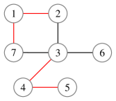
Consider a group of 7 robots, whose communication relation and conflict relation (at time tksubscript𝑡𝑘t_{k}) are depicted in Fig. 3. According to the proposed planning order assignment rule, the motion planning can be completed in 3 rounds, where robots 1 and 3 are in the first round, robots 2, 4 and 7 are in the second round, and robot 5 is in the third round. Note that no motion planning is required for robot 6 since robot 6 has no conflict neighbor.
Refer to caption
Figure 3: Communication and conflict graph, where both the black and red lines represent communication relation and the red lines represent conflict relation.

IV-E Motion planning

Before starting to plan, robot i𝑖i needs to wait for the updated plan from the set of neighbors that have higher priority than robot i𝑖i (i.e., j𝒴i(tk)𝑗subscript𝒴𝑖subscript𝑡𝑘j\in\mathcal{Y}_{i}(t_{k})) and consider them as moving obstacles. For those neighbors j𝒴i(tk)𝑗subscript𝒴𝑖subscript𝑡𝑘j\in\mathcal{Y}_{i}(t_{k}), denote by 𝝃j+([tk,))superscriptsubscript𝝃𝑗subscript𝑡𝑘{\bm{\xi}}_{j}^{+}([t_{k},\infty)) (correspondingly 𝝃j+([tk,))superscriptsubscript𝝃𝑗subscript𝑡𝑘{\bm{\xi}}_{j}^{+}([t_{k},\infty))) the updated trajectory (position trajectory) of robot j𝑗j at time tksubscript𝑡𝑘t_{k} and let tjfl+(tk)superscriptsubscript𝑡𝑗limit-from𝑓𝑙subscript𝑡𝑘t_{j}^{fl+}(t_{k}) be the first time that robot j𝑗j leaves its sensing area (pj(tk),R)subscript𝑝𝑗subscript𝑡𝑘𝑅\mathcal{B}(p_{j}(t_{k}),R) according to the updated position trajectory 𝒑j+([tk,))superscriptsubscript𝒑𝑗subscript𝑡𝑘{\bm{p}}_{j}^{+}([t_{k},\infty)). Then, similar to (30), one can define

Sj+(tk):=Q^(𝒑j+([tk,tjfl+]))assignsuperscriptsubscript𝑆𝑗subscript𝑡𝑘^𝑄superscriptsubscript𝒑𝑗subscript𝑡𝑘superscriptsubscript𝑡𝑗limit-from𝑓𝑙\displaystyle S_{j}^{+}(t_{k}):=\hat{Q}({\bm{p}}_{j}^{+}([t_{k},t_{j}^{fl+}]))

as the updated set of regions traversed by robot j𝑗j within (pj(tk),R)subscript𝑝𝑗subscript𝑡𝑘𝑅\mathcal{B}(p_{j}(t_{k}),R). For each X^lSj+(tk)subscript^𝑋𝑙superscriptsubscript𝑆𝑗subscript𝑡𝑘\hat{X}_{l}\in S_{j}^{+}(t_{k}), the time interval that robot j𝑗j occupies the region X^lsubscript^𝑋𝑙\hat{X}_{l} is given by Γ(𝒑j+([tk,tjfl+]),X^l)Γsuperscriptsubscript𝒑𝑗subscript𝑡𝑘superscriptsubscript𝑡𝑗limit-from𝑓𝑙subscript^𝑋𝑙\Gamma({\bm{p}}_{j}^{+}([t_{k},t_{j}^{fl+}]),{\hat{X}}_{l}). Supposing that Γ(𝒑j+([tk,tjfl+]),X^l)=l=1m^[a^l,b^l)Γsuperscriptsubscript𝒑𝑗subscript𝑡𝑘superscriptsubscript𝑡𝑗limit-from𝑓𝑙subscript^𝑋𝑙superscriptsubscript𝑙1^𝑚subscript^𝑎𝑙subscript^𝑏𝑙\Gamma({\bm{p}}_{j}^{+}([t_{k},t_{j}^{fl+}]),{\hat{X}}_{l})=\cup_{l=1}^{\hat{m}}[\hat{a}_{l},\hat{b}_{l}), where m^^𝑚\hat{m} is the number of disjoint intervals in Γ(𝒑j+([tk,tjfl+]),X^l)Γsuperscriptsubscript𝒑𝑗subscript𝑡𝑘superscriptsubscript𝑡𝑗limit-from𝑓𝑙subscript^𝑋𝑙\Gamma({\bm{p}}_{j}^{+}([t_{k},t_{j}^{fl+}]),{\hat{X}}_{l}). Denote by 𝒯j+(X^l)superscriptsubscript𝒯𝑗subscript^𝑋𝑙\mathcal{T}_{j}^{+}(\hat{X}_{l}) the time interval that robot j𝑗j reserves the area Resj(X^l)𝑅𝑒subscript𝑠𝑗subscript^𝑋𝑙Res_{j}(\hat{X}_{l}) according to the updated position trajectory 𝒑j+([tk,))superscriptsubscript𝒑𝑗subscript𝑡𝑘{\bm{p}}_{j}^{+}([t_{k},\infty)). Similarly to (33), it can be over-approximated by 𝒯j+(X^l):=l=1m^[a^l,b^l+Tibr].assignsuperscriptsubscript𝒯𝑗subscript^𝑋𝑙superscriptsubscript𝑙1^𝑚subscript^𝑎𝑙subscript^𝑏𝑙superscriptsubscript𝑇𝑖br\mathcal{T}_{j}^{+}(\hat{X}_{l}):=\cup_{l=1}^{\hat{m}}[\hat{a}_{l},\hat{b}_{l}+T_{i}^{\text{br}}].

Then, the trajectory planning problem (TPP) can be formulated as follows:

find𝝃i([tk,)),findsubscript𝝃𝑖subscript𝑡𝑘\displaystyle\text{find}\quad{{\bm{\xi}}_{i}}([t_{k},\infty)), (35a)
subject to
(7)and(8),7and8\displaystyle(\ref{x})\;\text{and}\;(\ref{cons}), (35b)
𝝃i([0,tk][tk,))φi,modelssubscript𝝃𝑖0subscript𝑡𝑘subscript𝑡𝑘subscript𝜑𝑖\displaystyle{\bm{\xi}}_{i}([0,t_{k}]\cup[t_{k},\infty))\models\varphi_{i}, (35c)
ψi(projl(𝝃i([tk,))))𝔽,subscript𝜓𝑖subscriptproj𝑙subscript𝝃𝑖subscript𝑡𝑘𝔽\displaystyle\psi_{i}(\texttt{proj}_{l}({\bm{\xi}}_{i}([t_{k},\infty))))\subset\mathbb{F}, (35d)
ψi(projl(ξi(t)))Resj(X^l)=,t𝒯j+(X^l),j𝒴i(tk),X^lSj+(tk).subscript𝜓𝑖subscriptproj𝑙subscript𝜉𝑖𝑡formulae-sequence𝑅𝑒subscript𝑠𝑗subscript^𝑋𝑙𝑡superscriptsubscript𝒯𝑗subscript^𝑋𝑙missing-subexpressionformulae-sequencefor-all𝑗subscript𝒴𝑖subscript𝑡𝑘for-allsubscript^𝑋𝑙superscriptsubscript𝑆𝑗subscript𝑡𝑘\displaystyle\begin{aligned} \psi_{i}(\texttt{proj}_{l}(\xi_{i}(t)))&\cap Res_{j}(\hat{X}_{l})=\emptyset,\;t\in\mathcal{T}_{j}^{+}(\hat{X}_{l}),\\ &\forall j\in\mathcal{Y}_{i}(t_{k}),\forall\hat{X}_{l}\in S_{j}^{+}(t_{k}).\end{aligned} (35e)

Constraints (35d) and (35e) guarantee respectively that there will be no robot-obstacle collisions and inter-robot collisions for robot i𝑖i.

When relatively simple specifications, e.g., reach-avoid type of tasks, are considered, various existing optimization toolboxes, e.g., IPOPT [33], ICLOCS2 [34], and algorithms, e.g., the configuration space-time search [35], the Hamilton-Jacobian reachability-based trajectory planning [36], RRTX [37], and the fast robot motion planner [38] can be utilized to solve (35). However, if the specifications are complex LTL formulas, the constraint (35c) is not easy to be verified online using the methods mentioned above (the PBA 𝒫isubscript𝒫𝑖\mathcal{P}_{i} can be used to verify (35c), however, it can not deal with the spatial-temporal collision avoidance constraint (35e) at the same time). Recently, an online RRT-based algorithm is proposed in [39] to generate local paths that guarantee the satisfaction of the global specification. Motivated by this work, an online motion replanning structure is proposed in this paper, which contains a local and a global trajectory generation algorithms.

Before proceeding, the following notations are required. Denote by

NIi(tk):={Resj(X^l),𝒯j+(X^l),\displaystyle NI_{i}(t_{k}):=\{Res_{j}(\hat{X}_{l}),\mathcal{T}_{j}^{+}(\hat{X}_{l}),
X^lSj+(tk),j𝒴i(tk)}\displaystyle\hskip 73.97733pt\forall\hat{X}_{l}\in S_{j}^{+}(t_{k}),\forall j\in\mathcal{Y}_{i}(t_{k})\} (36)

the set with respect to robot i𝑖i which contains all local trajectory information of higher priority neighbors at time tksubscript𝑡𝑘t_{k}. Given a state si𝕏^isubscript𝑠𝑖subscript^𝕏𝑖s_{i}\in\hat{\mathbb{X}}_{i}, define the function Bi:𝕏^i2Si:subscript𝐵𝑖subscript^𝕏𝑖superscript2subscript𝑆𝑖B_{i}:\hat{\mathbb{X}}_{i}\to 2^{S_{i}} as a map from a state si𝕏^isubscript𝑠𝑖subscript^𝕏𝑖s_{i}\in\hat{\mathbb{X}}_{i} to a subset of valid Büchi states which correspond to sisubscript𝑠𝑖s_{i} (i.e., Bi(si))β𝒫i(si)B_{i}(s_{i}))\subseteq\beta_{\mathcal{P}_{i}}(s_{i}), where β𝒫i(si)subscript𝛽subscript𝒫𝑖subscript𝑠𝑖\beta_{\mathcal{P}_{i}}(s_{i}) is defined in (5)). Function Bisubscript𝐵𝑖B_{i} is used to capture the fact that given a partial trajectory, not all Büchi states in β𝒫isubscript𝛽subscript𝒫𝑖\beta_{\mathcal{P}_{i}} are valid. At the task activation time 00, one has Bi(ξi(0))=β𝒫i(ξi(0))subscript𝐵𝑖subscript𝜉𝑖0subscript𝛽subscript𝒫𝑖subscript𝜉𝑖0B_{i}(\xi_{i}(0))=\beta_{\mathcal{P}_{i}}(\xi_{i}(0)). During the online implementation, Bi(ξi(tk)),tk>0subscript𝐵𝑖subscript𝜉𝑖subscript𝑡𝑘subscript𝑡𝑘0B_{i}(\xi_{i}(t_{k})),t_{k}>0 is updated by

Bi(ξi(tk))=β𝒫isubscript𝐵𝑖subscript𝜉𝑖subscript𝑡𝑘subscript𝛽subscript𝒫𝑖\displaystyle B_{i}(\xi_{i}(t_{k}))=\beta_{\mathcal{P}_{i}} (ξi(tk))subscript𝜉𝑖subscript𝑡𝑘\displaystyle(\xi_{i}(t_{k})) (37)
{Bi(ξi(tk1))𝙿𝚘𝚜𝚝(Bi(ξi(tk1)))}subscript𝐵𝑖subscript𝜉𝑖subscript𝑡𝑘1𝙿𝚘𝚜𝚝subscript𝐵𝑖subscript𝜉𝑖subscript𝑡𝑘1\displaystyle\cap\{B_{i}(\xi_{i}(t_{k-1}))\cup\verb"Post"(B_{i}(\xi_{i}(t_{k-1})))\}

where

Post(Bi(ξi(tk1)))=siBi(ξi(tk1))Post(si).Postsubscript𝐵𝑖subscript𝜉𝑖subscript𝑡𝑘1subscriptsubscript𝑠𝑖subscript𝐵𝑖subscript𝜉𝑖subscript𝑡𝑘1Postsubscript𝑠𝑖\texttt{Post}(B_{i}(\xi_{i}(t_{k-1})))=\cup_{s_{i}\in B_{i}(\xi_{i}(t_{k-1}))}\texttt{Post}(s_{i}). (38)

Firstly, the local trajectory generation process is outlined in Algorithm 3. At each time instant tksubscript𝑡𝑘t_{k}, Algorithm 3 takes the state ξi(tk)subscript𝜉𝑖subscript𝑡𝑘\xi_{i}(t_{k}) of robot i𝑖i, Bi(ξi(tk)),Post(Bi(ξi(tk)))subscript𝐵𝑖subscript𝜉𝑖subscript𝑡𝑘Postsubscript𝐵𝑖subscript𝜉𝑖subscript𝑡𝑘B_{i}(\xi_{i}(t_{k})),\texttt{Post}(B_{i}(\xi_{i}(t_{k}))), the offline computed PBA 𝒫isubscript𝒫𝑖\mathcal{P}_{i}, potential function V𝒫isubscript𝑉subscript𝒫𝑖V_{\mathcal{P}_{i}}, the set of static obstacles 𝕆𝕆\mathbb{O}, and the local trajectory information of higher priority neighbors, i.e., NIi(tk)𝑁subscript𝐼𝑖subscript𝑡𝑘NI_{i}(t_{k}) as input. The output is a local CTS 𝒯c,iL:=(SiL,Si,0L,APφi,c,iL,Lc,i)assignsuperscriptsubscript𝒯𝑐𝑖𝐿superscriptsubscript𝑆𝑖𝐿superscriptsubscript𝑆𝑖0𝐿𝐴subscript𝑃subscript𝜑𝑖superscriptsubscript𝑐𝑖𝐿subscript𝐿𝑐𝑖\mathcal{T}_{c,i}^{L}:=(S_{i}^{L},S_{i,0}^{L},AP_{\varphi_{i}},\rightarrow_{c,i}^{L},L_{c,i}) that is constructed incrementally and a leaf node ξifsuperscriptsubscript𝜉𝑖𝑓\xi_{i}^{f}.

Algorithm 3 localTrajectoryGeneration
1:ξi(tk),Bi(ξi(tk)),Post(Bi(ξi(tk)))subscript𝜉𝑖subscript𝑡𝑘subscript𝐵𝑖subscript𝜉𝑖subscript𝑡𝑘Postsubscript𝐵𝑖subscript𝜉𝑖subscript𝑡𝑘\xi_{i}(t_{k}),B_{i}(\xi_{i}(t_{k})),\texttt{Post}(B_{i}(\xi_{i}(t_{k}))), 𝒫i,V𝒫isubscript𝒫𝑖subscript𝑉subscript𝒫𝑖\mathcal{P}_{i},V_{\mathcal{P}_{i}}, 𝕆𝕆\mathbb{O}, and NIi(tk)𝑁subscript𝐼𝑖subscript𝑡𝑘NI_{i}(t_{k}).
2:A local transition system 𝒯c,iLsuperscriptsubscript𝒯𝑐𝑖𝐿\mathcal{T}_{c,i}^{L} and a leaf node ξifsuperscriptsubscript𝜉𝑖𝑓\xi_{i}^{f}.
3:Initialize 𝒯c,iL=(SiL,Si,0L,APφi,c,iL,Lc,i)superscriptsubscript𝒯𝑐𝑖𝐿superscriptsubscript𝑆𝑖𝐿superscriptsubscript𝑆𝑖0𝐿𝐴subscript𝑃subscript𝜑𝑖superscriptsubscript𝑐𝑖𝐿subscript𝐿𝑐𝑖\mathcal{T}_{c,i}^{L}=(S_{i}^{L},S_{i,0}^{L},AP_{\varphi_{i}},\rightarrow_{c,i}^{L},L_{c,i}) and ξif=superscriptsubscript𝜉𝑖𝑓\xi_{i}^{f}=\emptyset, where SiL=Si,0L=ξi(tk)superscriptsubscript𝑆𝑖𝐿superscriptsubscript𝑆𝑖0𝐿subscript𝜉𝑖subscript𝑡𝑘S_{i}^{L}=S_{i,0}^{L}=\xi_{i}(t_{k}) and c,iL=\rightarrow_{c,i}^{L}=\emptyset, 𝚂𝚝(ξi(tk))=0𝚂𝚝subscript𝜉𝑖subscript𝑡𝑘0\verb"St"(\xi_{i}(t_{k}))=0.
4:for k=1,,Nimax𝑘1superscriptsubscript𝑁𝑖k=1,\ldots,N_{i}^{\max} do,
5:     ξsgenerateSample(SAi(tk))subscript𝜉𝑠generateSample𝑆subscript𝐴𝑖subscript𝑡𝑘\xi_{s}\leftarrow\textit{generateSample}(SA_{i}(t_{k})),
6:     ξnnearest(SiL,ξs)subscript𝜉𝑛nearestsuperscriptsubscript𝑆𝑖𝐿subscript𝜉𝑠\xi_{n}\leftarrow\textit{nearest}(S_{i}^{L},\xi_{s}),
7:     Solve the optimization program 𝒫(ξn,ξs,τs)𝒫subscript𝜉𝑛subscript𝜉𝑠subscript𝜏𝑠\mathcal{P}(\xi_{n},\xi_{s},\tau_{s}), which returns (ξr,ui)subscript𝜉𝑟superscriptsubscript𝑢𝑖(\xi_{r},u_{i}^{*}),
8:     Bi(ξr)β𝒫i(ξr){Bi(ξn)𝙿𝚘𝚜𝚝(Bi(ξn))}subscript𝐵𝑖subscript𝜉𝑟subscript𝛽subscript𝒫𝑖subscript𝜉𝑟subscript𝐵𝑖subscript𝜉𝑛𝙿𝚘𝚜𝚝subscript𝐵𝑖subscript𝜉𝑛B_{i}(\xi_{r})\leftarrow\beta_{\mathcal{P}_{i}}(\xi_{r})\cap\{B_{i}(\xi_{n})\cup\verb"Post"(B_{i}(\xi_{n}))\},
9:     if Bi(ξr)V𝒯c,i(ξr,Bi(ξr))<subscript𝐵𝑖subscript𝜉𝑟subscript𝑉subscript𝒯𝑐𝑖subscript𝜉𝑟subscript𝐵𝑖subscript𝜉𝑟B_{i}(\xi_{r})\neq\emptyset\wedge V_{\mathcal{T}_{c,i}}(\xi_{r},B_{i}(\xi_{r}))<\infty then,
10:         𝕆i(tk)updateObstacle(𝕆,NIi(tk),[St(ξn)τs,\mathbb{O}_{i}(t_{k})\leftarrow\textit{updateObstacle}(\mathbb{O},NI_{i}(t_{k}),[\texttt{St}(\xi_{n})\tau_{s}, (St(ξn)+1)τs])(\texttt{St}(\xi_{n})+1)\tau_{s}]),
11:         if dist(projl([ξn,ξr]),𝕆i(tk))Dibrdistsubscriptproj𝑙subscript𝜉𝑛subscript𝜉𝑟subscript𝕆𝑖subscript𝑡𝑘superscriptsubscript𝐷𝑖br\texttt{dist}(\texttt{proj}_{l}([\xi_{n},\xi_{r}]),\mathbb{O}_{i}(t_{k}))\geq D_{i}^{\text{br}} then,
12:              SiLSiL{ξr};c,iL=c,iL{ξnuiξr}S_{i}^{L}\leftarrow S_{i}^{L}\cup\{\xi_{r}\};\rightarrow_{c,i}^{L}=\rightarrow_{c,i}^{L}\cup\{\xi_{n}\xrightarrow[]{u_{i}^{*}}\xi_{r}\},
13:              𝚂𝚝(ξs)𝚂𝚝(ξn)+1𝚂𝚝subscript𝜉𝑠𝚂𝚝subscript𝜉𝑛1\verb"St"(\xi_{s})\leftarrow\verb"St"(\xi_{n})+1,
14:         end if
15:     end if
16:     if projl(ξr)(projl(ξi(tk)),R)subscriptproj𝑙subscript𝜉𝑟subscriptproj𝑙subscript𝜉𝑖subscript𝑡𝑘𝑅\texttt{proj}_{l}(\xi_{r})\notin\mathcal{B}(\texttt{proj}_{l}(\xi_{i}(t_{k})),R)then
17:         k=Nimax+1𝑘superscriptsubscript𝑁𝑖1k=N_{i}^{\max}+1,
18:         ξifξrsuperscriptsubscript𝜉𝑖𝑓subscript𝜉𝑟\xi_{i}^{f}\leftarrow\xi_{r},
19:     end if
20:end for

In line 5, the optimization program 𝒫(ξn,ξs,τs)𝒫subscript𝜉𝑛subscript𝜉𝑠subscript𝜏𝑠\mathcal{P}(\xi_{n},\xi_{s},\tau_{s}) is given by

minui𝕌iξrξs,subscriptsubscript𝑢𝑖subscript𝕌𝑖normsubscript𝜉𝑟subscript𝜉𝑠\displaystyle\min_{u_{i}\in\mathbb{U}_{i}}\quad\|\xi_{r}-\xi_{s}\|, (39a)
subject to
ξi(0)=ξn,subscript𝜉𝑖0subscript𝜉𝑛\displaystyle\xi_{i}(0)=\xi_{n}, (39b)
ξn+0tFi(ξi(s),ui)𝑑s𝕏i,t[0,τs],formulae-sequencesubscript𝜉𝑛superscriptsubscript0𝑡subscript𝐹𝑖subscript𝜉𝑖𝑠subscript𝑢𝑖differential-d𝑠subscript𝕏𝑖for-all𝑡0subscript𝜏𝑠\displaystyle\xi_{n}+\int_{0}^{t}F_{i}(\xi_{i}(s),u_{i})ds\in\mathbb{X}_{i},\forall t\in[0,\tau_{s}], (39c)
ξr=ξn+0τsFi(ξi(s),ui)𝑑s,subscript𝜉𝑟subscript𝜉𝑛superscriptsubscript0subscript𝜏𝑠subscript𝐹𝑖subscript𝜉𝑖𝑠subscript𝑢𝑖differential-d𝑠\displaystyle\xi_{r}=\xi_{n}+\int_{0}^{\tau_{s}}F_{i}(\xi_{i}(s),u_{i})ds, (39d)

and the optimal solution is uisuperscriptsubscript𝑢𝑖u_{i}^{*}.

The root state of 𝒯c,iLsuperscriptsubscript𝒯𝑐𝑖𝐿\mathcal{T}_{c,i}^{L} is robot i𝑖i’s state ξi(tk)subscript𝜉𝑖subscript𝑡𝑘\xi_{i}(t_{k}). The function st:SiL:stsuperscriptsubscript𝑆𝑖𝐿\texttt{st}:S_{i}^{L}\to\mathbb{N} maps a state xSiL𝑥superscriptsubscript𝑆𝑖𝐿x\in S_{i}^{L} to the number of time steps needed to reach the root state ξi(tk)subscript𝜉𝑖subscript𝑡𝑘\xi_{i}(t_{k}). Initially, 𝒯c,iLsuperscriptsubscript𝒯𝑐𝑖𝐿\mathcal{T}_{c,i}^{L} contains one state ξi(tk)subscript𝜉𝑖subscript𝑡𝑘\xi_{i}(t_{k}) and 0 transitions, i.e., 𝚜𝚝(ξi(tk))=0𝚜𝚝subscript𝜉𝑖subscript𝑡𝑘0\verb"st"(\xi_{i}(t_{k}))=0, and the leaf node ξif=superscriptsubscript𝜉𝑖𝑓\xi_{i}^{f}=\emptyset (line 1). In each iteration (lines 2-18), a new state ξssubscript𝜉𝑠\xi_{s} is generated randomly from the set SAi(tk)𝑆subscript𝐴𝑖subscript𝑡𝑘SA_{i}(t_{k}) using the generateSample procedure (line 3), where SAi(tk)𝑆subscript𝐴𝑖subscript𝑡𝑘SA_{i}(t_{k}) is the sampling area around robot i𝑖i, given by

SAi(tk):={(p,ζ)𝕏i:p(projl(ξi(tk)),R+η)},assign𝑆subscript𝐴𝑖subscript𝑡𝑘conditional-set𝑝𝜁subscript𝕏𝑖𝑝subscriptproj𝑙subscript𝜉𝑖subscript𝑡𝑘𝑅𝜂\displaystyle SA_{i}(t_{k}):=\{(p,\zeta)\in\mathbb{X}_{i}:p\in\mathcal{B}(\texttt{proj}_{l}(\xi_{i}(t_{k})),R+\eta)\},

where η>0𝜂0\eta>0 is an offline chosen constant, which guarantees that there exists sSAi(tk)𝑠𝑆subscript𝐴𝑖subscript𝑡𝑘s\in SA_{i}(t_{k}) such that projl(s)(projl(ξi(tk)),R)subscriptproj𝑙𝑠subscriptproj𝑙subscript𝜉𝑖subscript𝑡𝑘𝑅\texttt{proj}_{l}(s)\notin\mathcal{B}(\texttt{proj}_{l}(\xi_{i}(t_{k})),R). This condition is essential for checking the terminal condition (line 15). The nearest function (line 4) is a standard RRT primitive [29] which returns the nearest state in SiLsuperscriptsubscript𝑆𝑖𝐿S_{i}^{L} to the new sample ξssubscript𝜉𝑠\xi_{s}. Then, one further finds, within the set of states that are reachable from ξnsubscript𝜉𝑛\xi_{n} at time τssubscript𝜏𝑠\tau_{s}, the closest one to the new sample ξssubscript𝜉𝑠\xi_{s}, i.e., ξrsubscript𝜉𝑟\xi_{r}, and the corresponding input uisuperscriptsubscript𝑢𝑖u_{i}^{*} (line 5). Here, τssubscript𝜏𝑠\tau_{s} is the sampling interval (the same one used for constructing the transition system 𝒯isubscript𝒯𝑖\mathcal{T}_{i} in Section IV-B3). Once ξrsubscript𝜉𝑟\xi_{r} is obtained, we further compute the subset of valid Büchi states which correspond to ξrsubscript𝜉𝑟\xi_{r}, i.e., Bi(ξr)subscript𝐵𝑖subscript𝜉𝑟B_{i}(\xi_{r}), according to (37) (line 6). After that, if both conditions Bi(ξr)subscript𝐵𝑖subscript𝜉𝑟B_{i}(\xi_{r})\neq\emptyset and V𝒯c,i(ξr,Bi(ξr))<subscript𝑉subscript𝒯𝑐𝑖subscript𝜉𝑟subscript𝐵𝑖subscript𝜉𝑟V_{\mathcal{T}_{c,i}}(\xi_{r},B_{i}(\xi_{r}))<\infty are satisfied (which guarantees that there exists a path, starting from ξrsubscript𝜉𝑟\xi_{r}, that reaches a self-reachable accepting state of 𝒫isubscript𝒫𝑖\mathcal{P}_{i}, recall Remark 1), obstacles that appear during the time interval [st(ξn)τs,(st(ξn)+1)τs]stsubscript𝜉𝑛subscript𝜏𝑠stsubscript𝜉𝑛1subscript𝜏𝑠[\texttt{st}(\xi_{n})\tau_{s},(\texttt{st}(\xi_{n})+1)\tau_{s}] are added into the workspace using the function updateObstacles (Algorithm 4). Finally, the state ξrsubscript𝜉𝑟\xi_{r} is added into SiLsuperscriptsubscript𝑆𝑖𝐿S_{i}^{L} and the transition relation ξnuiξrsuperscriptsubscript𝑢𝑖subscript𝜉𝑛subscript𝜉𝑟\xi_{n}\xrightarrow[]{u_{i}^{*}}\xi_{r} is added into c,iLsuperscriptsubscript𝑐𝑖𝐿\rightarrow_{c,i}^{L} if the distance between the line segment projl([ξn,ξr])subscriptproj𝑙subscript𝜉𝑛subscript𝜉𝑟\texttt{proj}_{l}([\xi_{n},\xi_{r}]) and the obstacles is no less than the braking distance of robot i𝑖i (lines 9-10), and then the time step needed for ξrsubscript𝜉𝑟\xi_{r} to reach the root state ξi(tk)subscript𝜉𝑖subscript𝑡𝑘\xi_{i}(t_{k}) is recorded (line 11). The algorithm is terminated when the local sampling tree reaches the outside of the sensing area of robot i𝑖i, and the leaf node ξifsuperscriptsubscript𝜉𝑖𝑓\xi_{i}^{f} is then given by the corresponding state ξrsubscript𝜉𝑟\xi_{r} (line 14-17).

Algorithm 4 updateObstacle
1:𝕆𝕆\mathbb{O}, NIi(tk)𝑁subscript𝐼𝑖subscript𝑡𝑘NI_{i}(t_{k}) and a time interval [t1,t2]subscript𝑡1subscript𝑡2[t_{1},t_{2}].
2:𝕆i(tk)subscript𝕆𝑖subscript𝑡𝑘\mathbb{O}_{i}(t_{k}).
3:𝕆i(tk)𝕆subscript𝕆𝑖subscript𝑡𝑘𝕆\mathbb{O}_{i}(t_{k})\leftarrow\mathbb{O},
4:for j𝒴i(tk)𝑗subscript𝒴𝑖subscript𝑡𝑘j\in\mathcal{Y}_{i}(t_{k})do
5:     for X^lSj+(tk)subscript^𝑋𝑙superscriptsubscript𝑆𝑗subscript𝑡𝑘\hat{X}_{l}\in S_{j}^{+}(t_{k})do
6:         if 𝒯j+(X^l)[tk+t1,tk+t2]superscriptsubscript𝒯𝑗subscript^𝑋𝑙subscript𝑡𝑘subscript𝑡1subscript𝑡𝑘subscript𝑡2\mathcal{T}_{j}^{+}(\hat{X}_{l})\cap[t_{k}+t_{1},t_{k}+t_{2}]\neq\emptysetthen
7:              𝕆i(tk)𝕆i(tk)(Resj(X^l)SAi(tk))subscript𝕆𝑖subscript𝑡𝑘subscript𝕆𝑖subscript𝑡𝑘𝑅𝑒subscript𝑠𝑗subscript^𝑋𝑙𝑆subscript𝐴𝑖subscript𝑡𝑘\mathbb{O}_{i}(t_{k})\leftarrow\mathbb{O}_{i}(t_{k})\cup(Res_{j}(\hat{X}_{l})\cap SA_{i}(t_{k})),
8:         end if
9:     end for
10:end for
Remark 6

The complexity of one iteration of Algorithm 3 is the same as for the standard RRT. The functions generateSample and nearest are standard RRT primitives (one can refer to [29] for more details). The complexity of the updateObstacle process (Algorithm 4) at time tksubscript𝑡𝑘t_{k} is 𝒪(1)𝒪1\mathcal{O}(1) since |𝒴i(tk)|N1subscript𝒴𝑖subscript𝑡𝑘𝑁1|\mathcal{Y}_{i}(t_{k})|\leq N-1 and |Sj+(tk)||Q^((pj(tk),R))|,jsuperscriptsubscript𝑆𝑗subscript𝑡𝑘^𝑄subscript𝑝𝑗subscript𝑡𝑘𝑅for-all𝑗|S_{j}^{+}(t_{k})|\leq|\hat{Q}(\mathcal{B}(p_{j}(t_{k}),R))|,\forall j, where |Q^((pj(tk),R))|^𝑄subscript𝑝𝑗subscript𝑡𝑘𝑅|\hat{Q}(\mathcal{B}(p_{j}(t_{k}),R))| represents the number of regions contained in the sensing area (pj(tk),R)subscript𝑝𝑗subscript𝑡𝑘𝑅\mathcal{B}(p_{j}(t_{k}),R). The computation of dist(projl([ξn,ξr]),𝕆i(tk))distsubscriptproj𝑙subscript𝜉𝑛subscript𝜉𝑟subscript𝕆𝑖subscript𝑡𝑘\texttt{dist}(\texttt{proj}_{l}([\xi_{n},\xi_{r}]),\mathbb{O}_{i}(t_{k})) can be formulated as a convex optimization problem and solved in 𝒪(1)𝒪1\mathcal{O}(1) since there is a limited number of obstacles in SAi(tk)𝑆subscript𝐴𝑖subscript𝑡𝑘SA_{i}(t_{k}) and each obstacle is of the form of a convex region. Moreover, the calculations of Bi(ξr)subscript𝐵𝑖subscript𝜉𝑟B_{i}(\xi_{r}) and V𝒯c,i(ξr,Bi(ξr))subscript𝑉subscript𝒯𝑐𝑖subscript𝜉𝑟subscript𝐵𝑖subscript𝜉𝑟V_{\mathcal{T}_{c,i}}(\xi_{r},B_{i}(\xi_{r})) are of the complexity of 𝒪(1)𝒪1\mathcal{O}(1) since 𝒫i,V𝒫isubscript𝒫𝑖subscript𝑉subscript𝒫𝑖\mathcal{P}_{i},V_{\mathcal{P}_{i}} are computed offline.

After the local CTS 𝒯c,iLsuperscriptsubscript𝒯𝑐𝑖𝐿\mathcal{T}_{c,i}^{L} is obtained, we further need to find a path, starting from the leaf node ξifsuperscriptsubscript𝜉𝑖𝑓\xi_{i}^{f}, that reaches one of the maximal self-reachable accepting states Fp,isuperscriptsubscript𝐹𝑝𝑖F_{p,i}^{*} of 𝒫isubscript𝒫𝑖\mathcal{P}_{i}. Define

Pi(ξif):=siBi(𝒯c,iL)(ξif,si)assignsubscript𝑃𝑖superscriptsubscript𝜉𝑖𝑓subscriptsubscript𝑠𝑖subscript𝐵𝑖superscriptsubscript𝒯𝑐𝑖𝐿superscriptsubscript𝜉𝑖𝑓subscript𝑠𝑖P_{i}(\xi_{i}^{f}):=\cup_{s_{i}\in B_{i}(\mathcal{T}_{c,i}^{L})}(\xi_{i}^{f},s_{i})

as the set of states in the PBA 𝒫isubscript𝒫𝑖\mathcal{P}_{i} that correspond to ξifsuperscriptsubscript𝜉𝑖𝑓\xi_{i}^{f}. Then, the global trajectory generation process is outlined in Algorithm 5. Algorithm 5 takes the set Pi(ξif)subscript𝑃𝑖superscriptsubscript𝜉𝑖𝑓P_{i}(\xi_{i}^{f}) and the the PBA 𝒫isubscript𝒫𝑖\mathcal{P}_{i} as input. It first finds the state pisuperscriptsubscript𝑝𝑖p_{i}^{*} in Pi(ξif)subscript𝑃𝑖superscriptsubscript𝜉𝑖𝑓P_{i}(\xi_{i}^{f}) that has the minimum potential (line 1). Then, if piFp,isuperscriptsubscript𝑝𝑖superscriptsubscript𝐹𝑝𝑖p_{i}^{*}\in F_{p,i}^{*}, the function DijksCycle(𝒫isubscript𝒫𝑖\mathcal{P}_{i}, source) (defined in [20]) is used to compute a shortest cycle from the source state back to itself (line 3); otherwise, the function DijksTargets(𝒫isubscript𝒫𝑖\mathcal{P}_{i}, source, targets) (defined in [20]) is used to compute a shortest path in 𝒫isubscript𝒫𝑖\mathcal{P}_{i} from “source” state to one of the state belonging to the set “targets” (line 5). The required path is then the projection of 𝒑isubscript𝒑𝑖\bm{p}_{i} on the state space of 𝒯c,isubscript𝒯𝑐𝑖\mathcal{T}_{c,i} (line 7).

Algorithm 5 globalTrajectoryGenration
1:Pi(ξif)subscript𝑃𝑖superscriptsubscript𝜉𝑖𝑓P_{i}(\xi_{i}^{f}) and 𝒫isubscript𝒫𝑖\mathcal{P}_{i}.
2:a path 𝝆isubscript𝝆𝑖\bm{\rho}_{i}.
3:pi=minpiPi(ξif){V𝒫i(pi)},superscriptsubscript𝑝𝑖subscriptsubscript𝑝𝑖subscript𝑃𝑖superscriptsubscript𝜉𝑖𝑓subscript𝑉subscript𝒫𝑖subscript𝑝𝑖p_{i}^{*}=\min_{p_{i}\in P_{i}(\xi_{i}^{f})}\{V_{\mathcal{P}_{i}}(p_{i})\},
4:if piFp,isuperscriptsubscript𝑝𝑖superscriptsubscript𝐹𝑝𝑖p_{i}^{*}\in F_{p,i}^{*} then
5:     𝒑iDijksCycle(𝒫i,pi)subscript𝒑𝑖DijksCyclesubscript𝒫𝑖superscriptsubscript𝑝𝑖\bm{p}_{i}\leftarrow\textit{DijksCycle}(\mathcal{P}_{i},p_{i}^{*}),
6:else
7:     𝒑iDijksTargets(𝒫i,pi,Fp,i)subscript𝒑𝑖DijksTargetssubscript𝒫𝑖superscriptsubscript𝑝𝑖superscriptsubscript𝐹𝑝𝑖\bm{p}_{i}\leftarrow\textit{DijksTargets}(\mathcal{P}_{i},p_{i}^{*},F_{p,i}^{*}),
8:end if
9:𝝆i=pj𝕏^i(𝒑i)subscript𝝆𝑖subscriptpjsubscript^𝕏𝑖subscript𝒑𝑖\bm{\rho}_{i}=\texttt{pj}_{\hat{\mathbb{X}}_{i}}(\bm{p}_{i}),

It is possible that after the maximum number of iterations (i.e., Nimaxsuperscriptsubscript𝑁𝑖N_{i}^{\max}), there exists no local path that reaches the outside of the sensing area of robot i𝑖i. In this case, the TPP (35) is considered infeasible, robot i𝑖i switches to Emerg mode and the braking controller (12) is applied. When robot i𝑖i is in Emerg mode, it will continue monitoring the environment (by updating 𝒯c,iLsuperscriptsubscript𝒯𝑐𝑖𝐿\mathcal{T}_{c,i}^{L}). Once a feasible local path is found, it will switch back to Free mode. The whole motion coordination process is summarized in Algorithm 6.

Algorithm 6 motionCoordination
1:(offline) Mi(X^l),X^lΞsubscript𝑀𝑖subscript^𝑋𝑙for-allsubscript^𝑋𝑙ΞM_{i}(\hat{X}_{l}),\forall\hat{X}_{l}\in\Xi, 𝒯c,isubscript𝒯𝑐𝑖\mathcal{T}_{c,i}, 𝖡i,𝒫isubscript𝖡𝑖subscript𝒫𝑖\mathsf{B}_{i},\mathcal{P}_{i}, and V𝒫isubscript𝑉subscript𝒫𝑖V_{\mathcal{P}_{i}}.
2:Real-time plan 𝝃i+([tk,)),tk0superscriptsubscript𝝃𝑖subscript𝑡𝑘subscript𝑡𝑘0{\bm{\xi}}_{i}^{+}([t_{k},\infty)),t_{k}\geq 0.
3:Initialize: 𝝃i([0,))𝝃i0superscriptsubscript𝝃𝑖0superscriptsubscript𝝃𝑖0{\bm{\xi}}_{i}^{-}([0,\infty))\leftarrow{\bm{\xi}}_{i}^{0}, Bi(ξi(0))β𝒫i(ξi(0))subscript𝐵𝑖subscript𝜉𝑖0subscript𝛽subscript𝒫𝑖subscript𝜉𝑖0B_{i}(\xi_{i}(0))\leftarrow\beta_{\mathcal{P}_{i}}(\xi_{i}(0)), Post(Bi(ξi(0)))siBi(ξi(0))Post(si),Postsubscript𝐵𝑖subscript𝜉𝑖0subscriptsubscript𝑠𝑖subscript𝐵𝑖subscript𝜉𝑖0Postsubscript𝑠𝑖\texttt{Post}(B_{i}(\xi_{i}(0)))\leftarrow\cup_{s_{i}\in B_{i}(\xi_{i}(0))}\texttt{Post}(s_{i}), and Robot i𝑖i is in Free mode.
4:while tk>0subscript𝑡𝑘0t_{k}>0 and φisubscript𝜑𝑖\varphi_{i} is not completed do,
5:      Compute Bi(ξi(tk))subscript𝐵𝑖subscript𝜉𝑖subscript𝑡𝑘B_{i}(\xi_{i}(t_{k})) and Post(Bi(ξi(tk)))Postsubscript𝐵𝑖subscript𝜉𝑖subscript𝑡𝑘\texttt{Post}(B_{i}(\xi_{i}(t_{k}))) according to (37) and (38),
6:     𝒩~i(tk)conflictDetection()subscript~𝒩𝑖subscript𝑡𝑘conflictDetection\tilde{\mathcal{N}}_{i}(t_{k})\leftarrow\textit{conflictDetection}(),
7:     if 𝒩~i(tk)subscript~𝒩𝑖subscript𝑡𝑘\tilde{\mathcal{N}}_{i}(t_{k})\neq\emptyset then
8:         Robot i𝑖i switches to Busy mode,
9:         𝒴i(t)planningOrderAssignment()subscript𝒴𝑖𝑡planningOrderAssignment\mathcal{Y}_{i}(t)\leftarrow\textit{planningOrderAssignment}(),
10:         (𝒯c,iL,ξif)localTrajectoryGeneration()superscriptsubscript𝒯𝑐𝑖𝐿superscriptsubscript𝜉𝑖𝑓localTrajectoryGeneration(\mathcal{T}_{c,i}^{L},\xi_{i}^{f})\leftarrow\textit{localTrajectoryGeneration}(),
11:         if ξifsuperscriptsubscript𝜉𝑖𝑓\xi_{i}^{f}\neq\emptysetthen
12:              𝝆iglobalTrajectoryGeneration()subscript𝝆𝑖globalTrajectoryGeneration\bm{\rho}_{i}\leftarrow\textit{globalTrajectoryGeneration}(),
13:               𝝃i+([tk,))DijksTargets(𝒯c,iL,ξi(tk),ξif)𝝆isuperscriptsubscript𝝃𝑖subscript𝑡𝑘DijksTargetssuperscriptsubscript𝒯𝑐𝑖𝐿subscript𝜉𝑖subscript𝑡𝑘superscriptsubscript𝜉𝑖𝑓subscript𝝆𝑖{\bm{\xi}}_{i}^{+}([t_{k},\infty))\leftarrow\textit{DijksTargets}(\mathcal{T}_{c,i}^{L},\xi_{i}(t_{k}),\xi_{i}^{f})\uplus\bm{\rho}_{i},
14:              Robot i𝑖i switches to Free mode,
15:         else
16:              Robot i𝑖i switches to Emerg mode,
17:              𝒖i𝒖ibr(ξi(tk))subscript𝒖𝑖superscriptsubscript𝒖𝑖brsubscript𝜉𝑖subscript𝑡𝑘{\bm{u}}_{i}\leftarrow{\bm{u}}_{i}^{\text{br}}(\xi_{i}(t_{k})),
18:              𝝃i+([tk,))𝝃i(ξi(tk),𝒖i,[0,))superscriptsubscript𝝃𝑖subscript𝑡𝑘subscript𝝃𝑖subscript𝜉𝑖subscript𝑡𝑘subscript𝒖𝑖0{\bm{\xi}}_{i}^{+}([t_{k},\infty))\leftarrow{\bm{\xi}}_{i}(\xi_{i}(t_{k}),{\bm{u}}_{i},[0,\infty)),
19:         end if
20:     else
21:         𝝃i+([tk,))𝝃i([tk,))superscriptsubscript𝝃𝑖subscript𝑡𝑘superscriptsubscript𝝃𝑖subscript𝑡𝑘{\bm{\xi}}_{i}^{+}([t_{k},\infty))\leftarrow{\bm{\xi}}_{i}^{-}([t_{k},\infty)),
22:     end if
23:end while

The following result shows hat safety is guaranteed under all circumstances.

Theorem 1 (Safety)

If the sensing radius of the robots satisfies R>2maxi𝒱{Dibr+Δmaxpi𝕎{p˙i}}𝑅2subscript𝑖𝒱superscriptsubscript𝐷𝑖brΔsubscriptsubscript𝑝𝑖𝕎normsubscript˙𝑝𝑖R>2\max_{i\in\mathcal{V}}\{D_{i}^{\text{br}}+\Delta\max_{p_{i}\in\mathbb{W}}\{\|\dot{p}_{i}\|\}\}, where ΔΔ\Delta is the conflict detection interval, then the resulting real-time plan of Algorithm 6 guarantees that there will be no obstacle-robot and inter-robot collisions for robot i𝑖i.

Proof: If the TPP (35) is feasible (robot i𝑖i will be in Free mode after the trajectory planning process), the local trajectory generation algorithm (Algorithm 3) and the global trajectory generation algorithm (Algorithm 5) guarantees that the constraints (35d) and (35e) of (35) are satisfied. That is to say, there will be no obstacle-robot and inter-robot collisions for robot i𝑖i. If the TPP (35) is infeasible (robot i𝑖i will switch to Emerg mode), robot i𝑖i would apply the braking controller 𝒖ibrsuperscriptsubscript𝒖𝑖br{\bm{u}}_{i}^{\text{br}} until it stops. Since R>2maxi𝒱{Dibr+Δmaxpi𝕎{p˙i}}𝑅2subscript𝑖𝒱superscriptsubscript𝐷𝑖brΔsubscriptsubscript𝑝𝑖𝕎normsubscript˙𝑝𝑖R>2\max_{i\in\mathcal{V}}\{D_{i}^{\text{br}}+\Delta\max_{p_{i}\in\mathbb{W}}\{\|\dot{p}_{i}\|\}\}, it guarantees that conflict between any pair of robots (i,j)𝑖𝑗(i,j) will be detected at the time that both robot i𝑖i and j𝑗j are outside of the braking area of the other. This means that there will be no inter-robot collision during the emergency stop process. On the other hand, when constructing 𝒯isubscript𝒯𝑖\mathcal{T}_{i}, one has ψi(projl(pi))𝔽,pi𝕏^iformulae-sequencesubscript𝜓𝑖subscriptproj𝑙subscript𝑝𝑖𝔽for-allsubscript𝑝𝑖subscript^𝕏𝑖\psi_{i}(\texttt{proj}_{l}(p_{i}))\subseteq\mathbb{F},\forall p_{i}\in\hat{\mathbb{X}}_{i}), i.e., dist(pi,𝕆)Dibr,pi𝕏^iformulae-sequencedistsubscript𝑝𝑖𝕆superscriptsubscript𝐷𝑖brfor-allsubscript𝑝𝑖subscript^𝕏𝑖\texttt{dist}(p_{i},\mathbb{O})\geq D_{i}^{\text{br}},\forall p_{i}\in\hat{\mathbb{X}}_{i}. Moreover, in the replanning process, it also requires that the distance between projl([ξn,ξr])subscriptproj𝑙subscript𝜉𝑛subscript𝜉𝑟\texttt{proj}_{l}([\xi_{n},\xi_{r}]) and static obstacles 𝕆𝕆\mathbb{O} is no less than Dibrsuperscriptsubscript𝐷𝑖brD_{i}^{\text{br}} (line 10, Algorithm 3). Therefore, there will be no obstacle-robot collision during the emergency stop process. Thus, no collision will occur for the whole process. \square

Theorem 2 (Correctness)

Let 𝛏irt([0,))superscriptsubscript𝛏𝑖rt0\bm{\xi}_{i}^{\text{rt}}([0,\infty)) be the real-time moving trajectory of robot i𝑖i. Then, 𝛏irt([0,))φimodelssuperscriptsubscript𝛏𝑖rt0subscript𝜑𝑖\bm{\xi}_{i}^{\text{rt}}([0,\infty))\models\varphi_{i} if robot i𝑖i never enters the Emerg mode or stays in Emerg mode for a finite time.

Proof: If robot i𝑖i never enters the Emerg mode, then one has from Algorithm 6 that robot i𝑖i never detects a conflict or the local trajectory generation algorithm (Algorithm 3) is always feasible for robot i𝑖i. Then, one can conclude that 𝝃irt([0,))φimodelssuperscriptsubscript𝝃𝑖rt0subscript𝜑𝑖\bm{\xi}_{i}^{\text{rt}}([0,\infty))\models\varphi_{i}. Otherwise, since robot i𝑖i stays in Emerg mode for a finite time, it means that robot i𝑖i can always switch back to Free mode, which implies the existence of a satisfying trajectory. In the light of Algorithm 6, the real-time moving trajectory 𝝃irt([0,))φimodelssuperscriptsubscript𝝃𝑖rt0subscript𝜑𝑖\bm{\xi}_{i}^{\text{rt}}([0,\infty))\models\varphi_{i}. \square

Remark 7

Due to the distributed fashion of the solution and the locally available information, the proposed motion coordination strategy is totally scalable in the sense that the computational complexity of the solution is not increasing with the number of robots. In addition, it is straightforward to extend the work to MRS scenarios where unknown static obstacles and moving obstacles are presented.

Remark 8

The workspace discretization, the planning order assignment, and the over-approximation of the braking area and time influence the completeness (the ability to find a solution when one exists) of the proposed solution. To improve completeness, online refinement of the discretization of the workspace, searching the space of the prioritization scheme (e.g., the randomized search approach with hill-climbing [40]), and less-conservative approximation of the braking area and time (using the real-time non-position information) can be utilized. The disadvantage is that the resulting approach will be computationally more complex.

IV-F Discussion of livelocks and deadlocks

In this subsection, the possibilities for livelocks and deadlocks are discussed. Firstly, the definitions of deadlock and livelock are given.

Definition 11

We say that a robot i𝑖i is in a deadlock if it remains in Emerg mode for an indefinite period (stop forever). We say that a robot i𝑖i is in a livelock if it is in Free mode (thus can move in the workspace) but unable to satisfy its specification.

Livelocks never occur. The reason is that according to our motion coordination algorithm (Algorithm 6), if a robot i𝑖i finds during execution that its specification is not satisfiable, then it will switch to Emerg mode and thus comes to a stop. In addition, it switches back to Free mode only when the task becomes satisfiable again. Therefore, there will be no livelocks.

Before discussing deadlocks, the definition of mutual satisfiability is provided. Denote by 𝒫G:=𝒫1𝒫|𝒱|assignsubscript𝒫𝐺tensor-productsubscript𝒫1subscript𝒫𝒱\mathcal{P}_{G}:=\mathcal{P}_{1}\otimes\ldots\otimes\mathcal{P}_{|\mathcal{V}|} the global PBA, which is the product of all local PBAs 𝒫i,i𝒱subscript𝒫𝑖𝑖𝒱\mathcal{P}_{i},i\in\mathcal{V}.

Definition 12

We say that the set of LTL specifications {φ1,,φ|𝒱|}subscript𝜑1subscript𝜑𝒱\{\varphi_{1},\ldots,\varphi_{|\mathcal{V}|}\} is mutually satisfiable if there exists an accepting run 𝐩Gsubscript𝐩𝐺\bm{p}_{G} of 𝒫Gsubscript𝒫𝐺\mathcal{P}_{G} such that

ϕi(projl(ξi(t)))ϕj(projl(ξj(t)))=,subscriptitalic-ϕ𝑖subscriptproj𝑙subscript𝜉𝑖𝑡subscriptitalic-ϕ𝑗subscriptproj𝑙subscript𝜉𝑗𝑡\displaystyle\phi_{i}(\texttt{proj}_{l}({\xi}_{i}(t)))\cap\phi_{j}(\texttt{proj}_{l}(\xi_{j}(t)))=\emptyset,
i,j𝒱,ij,t0,formulae-sequencefor-all𝑖𝑗𝒱formulae-sequence𝑖𝑗for-all𝑡0\displaystyle\hskip 99.58464pt\forall i,j\in\mathcal{V},i\neq j,\forall t\geq 0,

where 𝛏isubscript𝛏𝑖\bm{\xi}_{i} is the projection of 𝐩Gsubscript𝐩𝐺\bm{p}_{G} onto the local CTS 𝒯isubscript𝒯𝑖\mathcal{T}_{i}.

When the set of LTL specifications {φ1,,φ|𝒱|}subscript𝜑1subscript𝜑𝒱\{\varphi_{1},\ldots,\varphi_{|\mathcal{V}|}\} is not mutually satisfiable, deadlocks can happen because the LTL specifications of two or multiple robots can not be satisfied simultaneously in a collision-free manner. This type of deadlocks is unresolvable. When the set of LTL specifications {φ1,,φ|𝒱|}subscript𝜑1subscript𝜑𝒱\{\varphi_{1},\ldots,\varphi_{|\mathcal{V}|}\} is mutually satisfiable, deadlocks can also happen due to the incompleteness of the motion coordination algorithm (Remark 8) or the locally available information of the neighboring robots. Existing methods such as path refinement [41] and simultaneous trajectory planning [42] (instead of the sequential trajectory planning used in this work), can be invoked to resolve this type of deadlocks. To detect a possible deadlock, one can a priori specify a maximum time tmaxsubscript𝑡t_{\max} allowed for a robot to stay in Emerg mode.

V Case studies

In this section, two case studies are provided to illustrate the effectiveness and computational tractability of the proposed framework. All simulations are carried out in Matlab 2018b on a Dell laptop with Windows 10, Intel i7-6600U CPU2.80GHz and 16.0 GB RAM.

V-A Example 1

Consider a MRS consisting of N=4𝑁4N=4 robots, the dynamics of robot i𝑖i is given by (17), and the velocity and input constraints are given by (18). For robots i{1,2}𝑖12i\in\{1,2\}, one has that vi,max=1m/ssubscript𝑣𝑖1msv_{i,\max}=1{\rm m/s}, ωi,max=0.5rad/ssubscript𝜔𝑖0.5rads\omega_{i,\max}=0.5{\rm rad/s}, and ai,max=2m/s2subscript𝑎𝑖2msuperscripts2a_{i,\max}=2{\rm m/s^{2}}. For robots i{3,4}𝑖34i\in\{3,4\}, one has that vi,max=1m/ssubscript𝑣𝑖1msv_{i,\max}=1{\rm m/s}, ωi,max=0.5rad/ssubscript𝜔𝑖0.5rads\omega_{i,\max}=0.5{\rm rad/s}, and ai,max=1.5m/s2subscript𝑎𝑖1.5msuperscripts2a_{i,\max}=1.5{\rm m/s^{2}}. Then, using the braking controller (21), one can get that Tibr=0.5s,Dibr=0.25m,i=1,2formulae-sequencesuperscriptsubscript𝑇𝑖br0.5sformulae-sequencesuperscriptsubscript𝐷𝑖br0.25m𝑖12T_{i}^{\text{br}}=0.5{\rm s},D_{i}^{\text{br}}=0.25{\rm m},i=1,2 and Tibr=0.5s,Dibr=0.33m,i=3,4formulae-sequencesuperscriptsubscript𝑇𝑖br0.5sformulae-sequencesuperscriptsubscript𝐷𝑖br0.33m𝑖34T_{i}^{\text{br}}=0.5{\rm s},D_{i}^{\text{br}}=0.33{\rm m},i=3,4. The sensing radius of each robot is R=3.5m𝑅3.5mR=3.5{\rm m} and the conflict detection period is Δ=0.1sΔ0.1s\Delta=0.1{\rm s}. Then one has that R>2maxi𝒱{Dibr+Δvi,max}𝑅2subscript𝑖𝒱superscriptsubscript𝐷𝑖brΔsubscript𝑣𝑖R>2\max_{i\in\mathcal{V}}\{D_{i}^{\text{br}}+\Delta v_{i,\max}\}.

As shown in Fig. 4, the workspace 𝕎𝕎\mathbb{W} we consider is a 20×20m22020superscriptm220\times 20{\rm m^{2}} square, where the gray areas, marked as O1,O2,O3subscript𝑂1subscript𝑂2subscript𝑂3O_{1},O_{2},O_{3}, represent three static obstacles, the colored small circles represent the initial position of the robots, and the light blue areas, marked as T1,T2,,T5subscript𝑇1subscript𝑇2subscript𝑇5T_{1},T_{2},\ldots,T_{5}, represent a set of target regions in the workspace. Initially, θi=0,vi(0)=0,iformulae-sequencesubscript𝜃𝑖0subscript𝑣𝑖00for-all𝑖\theta_{i}=0,v_{i}(0)=0,\forall i.

Refer to caption
Figure 4: The workspace for the group of robots in Example 1.

Each robot is assigned to persistently survey two of the target regions in the workspace. In LTL formulas, the specification for each robot is given by

  • φ1=(𝕎¬𝕆)T1T2subscript𝜑1𝕎𝕆subscript𝑇1subscript𝑇2\varphi_{1}=\square(\mathbb{W}\wedge\neg\mathbb{O})\wedge\square\lozenge T_{1}\wedge\square\lozenge T_{2},

  • φ2=(𝕎¬𝕆)T1T5subscript𝜑2𝕎𝕆subscript𝑇1subscript𝑇5\varphi_{2}=\square(\mathbb{W}\wedge\neg\mathbb{O})\wedge\square\lozenge T_{1}\wedge\square\lozenge T_{5},

  • φ3=(𝕎¬𝕆)T2T4subscript𝜑3𝕎𝕆subscript𝑇2subscript𝑇4\varphi_{3}=\square(\mathbb{W}\wedge\neg\mathbb{O})\wedge\square\lozenge T_{2}\wedge\square\lozenge T_{4},

  • φ4=(𝕎¬𝕆)T3T5subscript𝜑4𝕎𝕆subscript𝑇3subscript𝑇5\varphi_{4}=\square(\mathbb{W}\wedge\neg\mathbb{O})\wedge\square\lozenge T_{3}\wedge\square\lozenge T_{5},

where 𝕆=O1O2O3𝕆subscript𝑂1subscript𝑂2subscript𝑂3\mathbb{O}=O_{1}\cup O_{2}\cup O_{3}. Firstly, a rough cell decomposition is given over the workspace 𝕎𝕎\mathbb{W} such that Assumption 1 is satisfied. Then, for each cell Xl𝕎𝕆subscript𝑋𝑙𝕎𝕆X_{l}\subset\mathbb{W}\setminus\mathbb{O}, a grid representation with grid size 0.5m0.5m0.5{\rm m} is implemented as a finer workspace discretization. The NBA 𝖡isubscript𝖡𝑖\mathsf{B}_{i} associated with φi,isubscript𝜑𝑖for-all𝑖\varphi_{i},\forall i has 3 states and 8 edges by [24]. The CTS 𝒯isubscript𝒯𝑖\mathcal{T}_{i} and the PBA 𝒫isubscript𝒫𝑖\mathcal{P}_{i} for each robot are constructed using LTLCon toolbox [43]. Finally, the map Misubscript𝑀𝑖M_{i} (defined in (27)) and potential function for each 𝒫isubscript𝒫𝑖\mathcal{P}_{i} (Definition 6) are computed.

Refer to caption
Refer to caption
Refer to caption
Refer to caption
Figure 5: The real-time position trajectory of each robot, where the small circle represents the initial position of each robot.
Refer to caption
Figure 6: The evolution of the position trajectories with respect to time.
Refer to caption
Refer to caption
Refer to caption
Refer to caption
Figure 7: The local motion replanning between different conflict robots. The circle, marked with a dotted line, represents the sensing area of the robot that replans, the dashed lines represent the planned local position trajectories of the robots, the colored small squares represent its (over-approximated) braking areas, the yellow squares represent the conflict region, and the solid line represents the replanned local position trajectory.

Initially, each robot i𝑖i finds a safely satisfying trajectory 𝝃i0superscriptsubscript𝝃𝑖0\bm{\xi}_{i}^{0} (in the form of prefix-suffix). Then, the motion coordination algorithm (Algorithm 6) is implemented for each robot during online execution. The real-time position trajectory of each robot is depicted in Fig. 5 (a)-(d), respectively. It can be seen that during the simulation time [0,120]s0120s[0,120]{\rm s}, the surveillance task of each robot is satisfied at least once. Fig. 6 shows the evolution of the position trajectories of all robots with respect to time. One can see that the real-time position trajectories are collision-free. During the simulation time, conflicts are detected in total 11 times. Whenever conflicts are detected, the planning order assignment module and the trajectory planning module are activated to resolve the conflicts. In Fig. 7 (a)-(d), 4 cases of local motion replanning are depicted, respectively. In each of the subfigures, the circle, marked as dotted line, represents the sensing area of the robot that replans, the dashed lines represent the planned local position trajectories of the robots, the colored small squares represent its (over-approximated) braking areas, the yellow squares represent the conflict region, and the solid line represents the replanned local position trajectory. A video recording of the real-time implementation can be found here: https://youtu.be/7Xjt62psZe0.

The real-time evolution of velocity visubscript𝑣𝑖v_{i} and inputs (ai,ωi)subscript𝑎𝑖subscript𝜔𝑖(a_{i},\omega_{i}) of each robot i𝑖i are plotted in Fig. 8 and Fig. 9, respectively. One can see that the velocity constraints and the input constraints are satisfied by all robots at any time.
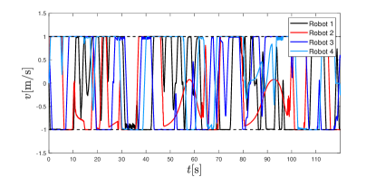
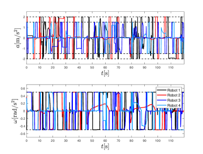
Refer to caption
Figure 8: The real-time evolution of velocity visubscript𝑣𝑖v_{i} for each robot, where vi,max=1m/s,i{1,2,3,4}formulae-sequencesubscript𝑣𝑖1ms𝑖1234v_{i,\max}=1{\rm m/s},i\in\{1,2,3,4\}.
Refer to caption
Figure 9: The real-time evolution of inputs (ai,ωi)subscript𝑎𝑖subscript𝜔𝑖(a_{i},\omega_{i}) for each robot, where ai,max=2m/s2,ωi,max=0.5rad/s,i{1,2}formulae-sequencesubscript𝑎𝑖2msuperscripts2formulae-sequencesubscript𝜔𝑖0.5rads𝑖12a_{i,\max}=2{\rm m/s^{2}},\omega_{i,\max}=0.5{\rm rad/s},i\in\{1,2\} and ai,max=1.5m/s2,ωi,max=0.5rad/s,i{3,4}formulae-sequencesubscript𝑎𝑖1.5msuperscripts2formulae-sequencesubscript𝜔𝑖0.5rads𝑖34a_{i,\max}=1.5{\rm m/s^{2}},\omega_{i,\max}=0.5{\rm rad/s},i\in\{3,4\}.

Finally, we report the computation times of this example. For the 11 local replannings, the average computation time is 1.51s1.51s1.51{\rm s} and the maximum computation time is 3.30s3.30s3.30{\rm s}. The computation of the global trajectory (Algorithm 5) is quite fast (less than 0.1s0.1s0.1{\rm s}). Note that after the local and global trajectories are obtained, the toolbox ICLOCS2 [34] is further employed for trajectory smoothness. In addition, it is worth to point out that we have tried 10 different sets of initial states and specifications for the group of robots, and we find that the initial states and the specifications have little effect on the average time and maximum time of local replanning. There is no change of order of magnitude in the computation time for all trials.

V-B Example 2

This example aims at demonstrating the computational tractability of the approach with respect to the number of robots.
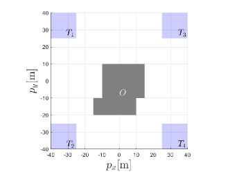
Refer to caption
Figure 10: The workspace for the group of robots in Example 2.

As depicted in Fig. 10, the workspace 𝕎𝕎\mathbb{W} considered now is a 80×80m28080superscriptm280\times 80{\rm m^{2}} square, where the gray area, marked as O𝑂O is the obstacle, and the light blue areas, marked as T1,T2,,T4subscript𝑇1subscript𝑇2subscript𝑇4T_{1},T_{2},\ldots,T_{4}, represent 4 target regions in the workspace. We consider respectively the cases where 2, 4, 8 and 16 robots are working in the workspace. The dynamics of robot i𝑖i is given by a double-integrator, i.e.,

p˙isubscript˙𝑝𝑖\displaystyle\dot{p}_{i} =\displaystyle= visubscript𝑣𝑖\displaystyle v_{i}
v˙isubscript˙𝑣𝑖\displaystyle\dot{v}_{i} =\displaystyle= ui,isubscript𝑢𝑖for-all𝑖\displaystyle u_{i},\forall i

where pi,vi,ui2subscript𝑝𝑖subscript𝑣𝑖subscript𝑢𝑖superscript2p_{i},v_{i},u_{i}\in\mathbb{R}^{2} represent the position, velocity, and input of robot i𝑖i, respectively. The velocity and input of robot i𝑖i are subject to the hard constraints

vi(t)vi,max=3m/s,normsubscript𝑣𝑖𝑡subscript𝑣𝑖3ms\displaystyle||v_{i}(t)||\leq v_{i,\max}=3{\rm m/s},
ui(t)ui,max=6m/s2,i.formulae-sequencenormsubscript𝑢𝑖𝑡subscript𝑢𝑖6msuperscripts2for-all𝑖\displaystyle||u_{i}(t)||\leq u_{i,\max}=6{\rm m/s^{2}},\forall i.

The braking controller 𝒖ibrsuperscriptsubscript𝒖𝑖br\bm{u}_{i}^{\text{br}} is designed as

uibr(t)={ui,maxvi(t)vi(t),ifvi(t)0,02,ifvi(t)=0.u_{i}^{\text{br}}(t)=\left\{\begin{aligned} -u_{i,\max}\frac{v_{i}(t)}{||v_{i}(t)||},&\quad\text{if}\;||v_{i}(t)||\neq 0,\\ 0_{2}\quad\quad\quad,&\quad\text{if}\;||v_{i}(t)||=0.\end{aligned}\right.

Then, one can derive the braking time Tibr=vi,max/ui,max=0.5ssuperscriptsubscript𝑇𝑖brnormsubscript𝑣𝑖normsubscript𝑢𝑖0.5sT_{i}^{\text{br}}={||v_{i,\max}||}/{||u_{i,\max}||}=0.5{\rm s} and the braking distance Dibr=vi,max2/2ui,max=0.75m,iformulae-sequencesuperscriptsubscript𝐷𝑖brsuperscriptnormsubscript𝑣𝑖22normsubscript𝑢𝑖0.75mfor-all𝑖D_{i}^{\text{br}}=||v_{i,\max}||^{2}/2||u_{i,\max}||=0.75{\rm m},\forall i. The sensing radius of each robot is R=6m𝑅6mR=6{\rm m} and the conflict detection period is Δ=0.1sΔ0.1s\Delta=0.1{\rm s}.

For simplicity, we consider that half of the robots are assigned to persistently survey target regions T1subscript𝑇1T_{1} and T3subscript𝑇3T_{3}, and the other half are assigned to persistently survey target regions T2subscript𝑇2T_{2} and T4subscript𝑇4T_{4}. In LTL formulas, the specification for each robot is given by

  • φi=(𝕎¬O)T1T4,i=1,3,,15,formulae-sequencesubscript𝜑𝑖𝕎𝑂subscript𝑇1subscript𝑇4𝑖1315\varphi_{i}=\square(\mathbb{W}\wedge\neg O)\wedge\square\lozenge T_{1}\wedge\square\lozenge T_{4},i=1,3,\ldots,15,

  • φi=(𝕎¬O)T2T3,i=2,4,,16formulae-sequencesubscript𝜑𝑖𝕎𝑂subscript𝑇2subscript𝑇3𝑖2416\varphi_{i}=\square(\mathbb{W}\wedge\neg O)\wedge\square\lozenge T_{2}\wedge\square\lozenge T_{3},i=2,4,\ldots,16.

A grid representation with grid size 2m2m2{\rm m} is implemented as the workspace discretization.

For each of the cases (2, 4, 8 or 16 robots), the simulation time is 150s150s150{\rm s}. The simulation results are summarized in TABLE II, where the total number of conflict times (CT), the average computation time for local replanning (ATLR), and the maximum computation time for local replanning (MTLR) are reported. It can be seen that as the number of robots grows (exponentially), the CT grows significantly (the reason is that the workspace is the same). The ATLR and MTLR grow, but not significantly. One can see that even when there are 16 robots, the local replanning is still efficient.

TABLE II: The CT, ATLR, and MTLR with respect to the number of robots.
number of robots CT ATLR (s) MTLR (s)
2 0 - -
4 6 0.23 2.99
8 19 0.31 3.80
16 72 0.63 4.94

VI Conclusion

In this paper, the online MRMC problem for a group of mobile robots moving in a shared workspace was considered. Under the assumptions that each robot has only local view and local information, and subject to both state and input constraints, a fully distributed motion coordination strategy was proposed for steering individual robots in a common workspace, where each robot is assigned a LTL specification. It was shown that the proposed strategy can guarantee collision-free motion of each robot. In the future, MRMC under both team and individual tasks will be of interest. In addition, the experimental validation of the proposed strategy by real-world robots will be pursued.

References

  • [1] Z. Yan, N. Jouandeau, and A. A. Cherif, “A survey and analysis of multi-robot coordination,” International Journal of Advanced Robotic Systems, vol. 10, no. 12, p. 399, 2013.
  • [2] L. E. Parker, “Path planning and motion coordination in multiple mobile robot teams,” Encyclopedia of complexity and system science, pp. 5783–5800, 2009.
  • [3] O. Khatib, “Real-time obstacle avoidance for manipulators and mobile robots,” in Autonomous robot vehicles.   Springer, 1986, pp. 396–404.
  • [4] D. Panagou, “Motion planning and collision avoidance using navigation vector fields,” in 2014 IEEE International Conference on Robotics and Automation (ICRA), 2014, pp. 2513–2518.
  • [5] L. Gracia, F. Garelli, and A. Sala, “Reactive sliding-mode algorithm for collision avoidance in robotic systems,” IEEE Transactions on Control Systems Technology, vol. 21, no. 6, pp. 2391–2399, 2013.
  • [6] H. Farivarnejad, S. Wilson, and S. Berman, “Decentralized sliding mode control for autonomous collective transport by multi-robot systems,” in 2016 IEEE 55th Conference on Decision and Control (CDC), 2016, pp. 1826–1833.
  • [7] L. Wang, A. D. Ames, and M. Egerstedt, “Safety barrier certificates for collisions-free multirobot systems,” IEEE Transactions on Robotics, vol. 33, no. 3, pp. 661–674, 2017.
  • [8] P. Glotfelter, J. Cortés, and M. Egerstedt, “Nonsmooth barrier functions with applications to multi-robot systems,” IEEE control systems letters, vol. 1, no. 2, pp. 310–315, 2017.
  • [9] L. Pallottino, V. G. Scordio, A. Bicchi, and E. Frazzoli, “Decentralized cooperative policy for conflict resolution in multivehicle systems,” IEEE Transactions on Robotics, vol. 23, no. 6, pp. 1170–1183, 2007.
  • [10] G. A. Bekey, Autonomous Robots: from Biological Inspiration to Implementation and Control.   MIT press, 2005.
  • [11] K. Azarm and G. Schmidt, “Conflict-free motion of multiple mobile robots based on decentralized motion planning and negotiation,” in Proceedings of International Conference on Robotics and Automation, vol. 4, 1997, pp. 3526–3533.
  • [12] Y. Guo and L. E. Parker, “A distributed and optimal motion planning approach for multiple mobile robots,” in Proceedings 2002 IEEE International Conference on Robotics and Automation (Cat. No. 02CH37292), vol. 3, 2002, pp. 2612–2619.
  • [13] W. Sheng, Q. Yang, J. Tan, and N. Xi, “Distributed multi-robot coordination in area exploration,” Robotics and Autonomous Systems, vol. 54, no. 12, pp. 945–955, 2006.
  • [14] C. Liu, C.-W. Lin, S. Shiraishi, and M. Tomizuka, “Distributed conflict resolution for connected autonomous vehicles,” IEEE Transactions on Intelligent Vehicles, vol. 3, no. 1, pp. 18–29, 2017.
  • [15] A. Ulusoy, S. L. Smith, X. C. Ding, C. Belta, and D. Rus, “Optimality and robustness in multi-robot path planning with temporal logic constraints,” The International Journal of Robotics Research, vol. 32, no. 8, pp. 889–911, 2013.
  • [16] Y. Shoukry, P. Nuzzo, A. Balkan, I. Saha, A. L. Sangiovanni-Vincentelli, S. A. Seshia, G. J. Pappas, and P. Tabuada, “Linear temporal logic motion planning for teams of underactuated robots using satisfiability modulo convex programming,” in 2017 IEEE 56th annual conference on decision and control (CDC).   IEEE, 2017, pp. 1132–1137.
  • [17] Y. E. Sahin, P. Nilsson, and N. Ozay, “Multirobot coordination with counting temporal logics,” IEEE Transactions on Robotics, 2019.
  • [18] Y. Kantaros and M. M. Zavlanos, “Stylus*: A temporal logic optimal control synthesis algorithm for large-scale multi-robot systems,” The International Journal of Robotics Research, vol. 39, no. 7, pp. 812–836, 2020.
  • [19] J. Alonso-Mora, J. A. DeCastro, V. Raman, D. Rus, and H. Kress-Gazit, “Reactive mission and motion planning with deadlock resolution avoiding dynamic obstacles,” Autonomous Robots, vol. 42, no. 4, pp. 801–824, 2018.
  • [20] M. Guo and D. V. Dimarogonas, “Multi-agent plan reconfiguration under local LTL specifications,” The International Journal of Robotics Research, vol. 34, no. 2, pp. 218–235, 2015.
  • [21] P. Yu and D. V. Dimarogonas, “A fully distributed motion coordination strategy for multi-robot systems with local information,” arXiv preprint arXiv:2004.10437, 2020.
  • [22] C. Baier and J.-P. Katoen, Principles of Model Checking.   MIT press, 2008.
  • [23] J. R. Büchi, “On a decision method in restricted second order arithmetic,” in The Collected Works of J. Richard Büchi.   Springer, 1990, pp. 425–435.
  • [24] P. Gastin and D. Oddoux, “Fast LTL to Büchi automata translation,” in International Conference on Computer Aided Verification.   Springer, 2001, pp. 53–65.
  • [25] C. I. Vasile and C. Belta, “Sampling-based temporal logic path planning,” in 2013 IEEE/RSJ International Conference on Intelligent Robots and Systems, 2013, pp. 4817–4822.
  • [26] E. A. Emerson, “Temporal and modal logic,” in Formal Models and Semantics.   Elsevier, 1990, pp. 995–1072.
  • [27] J.-C. Latombe, Robot Motion Planning.   Springer Science & Business Media, 2012, vol. 124.
  • [28] S. Bhattacharya, V. Kumar, and M. Likhachev, “Search-based path planning with homotopy class constraints.” in AAAI, 2010, pp. 1230–1237.
  • [29] S. M. LaValle and J. J. Kuffner, “Rapidly-exploring random trees: Progress and prospects,” Algorithmic and computational robotics: new directions, no. 5, pp. 293–308, 2001.
  • [30] M. M. Quottrup, T. Bak, and R. Zamanabadi, “Multi-robot planning: A timed automata approach,” in IEEE International Conference on Robotics and Automation, 2004. Proceedings. ICRA’04. 2004, vol. 5, 2004, pp. 4417–4422.
  • [31] T. M. Howard, C. J. Green, and A. Kelly, “Receding horizon model-predictive control for mobile robot navigation of intricate paths,” in Field and Service Robotics.   Springer, 2010, pp. 69–78.
  • [32] J. Schulman, J. Ho, A. X. Lee, I. Awwal, H. Bradlow, and P. Abbeel, “Finding locally optimal, collision-free trajectories with sequential convex optimization.” in Robotics: science and systems, vol. 9, no. 1.   Citeseer, 2013, pp. 1–10.
  • [33] L. T. Biegler and V. M. Zavala, “Large-scale nonlinear programming using ipopt: An integrating framework for enterprise-wide dynamic optimization,” Computers & Chemical Engineering, vol. 33, no. 3, pp. 575–582, 2009.
  • [34] Y. Nie, O. Faqir, and E. C. Kerrigan, “ICLOCS2: Solve your optimal control problems with less pain,” 2018.
  • [35] D. Parsons and J. Canny, “A motion planner for multiple mobile robots,” in Proceedings., IEEE International Conference on Robotics and Automation, 1990, pp. 8–13.
  • [36] M. Chen, S. Bansal, J. F. Fisac, and C. J. Tomlin, “Robust sequential trajectory planning under disturbances and adversarial intruder,” IEEE Transactions on Control Systems Technology, vol. 27, no. 4, pp. 1566–1582, 2018.
  • [37] M. Otte and E. Frazzoli, “RRTX: Asymptotically optimal single-query sampling-based motion planning with quick replanning,” The International Journal of Robotics Research, vol. 35, no. 7, pp. 797–822, 2016.
  • [38] H.-C. Lin, C. Liu, and M. Tomizuka, “Fast robot motion planning with collision avoidance and temporal optimization,” in 2018 15th International Conference on Control, Automation, Robotics and Vision (ICARCV), 2018, pp. 29–35.
  • [39] C. I. Vasile and C. Belta, “Reactive sampling-based temporal logic path planning,” in 2014 IEEE International Conference on Robotics and Automation (ICRA), 2014, pp. 4310–4315.
  • [40] M. Bennewitz, W. Burgard, and S. Thrun, “Finding and optimizing solvable priority schemes for decoupled path planning techniques for teams of mobile robots,” Robotics and autonomous systems, vol. 41, no. 2-3, pp. 89–99, 2002.
  • [41] M. G. Atia, O. Salah, and H. Ei-Hussieny, “Ogpr: An obstacle-guided path refinement approach for mobile robot path planning,” in 2018 IEEE International Conference on Robotics and Biomimetics (ROBIO), 2018, pp. 844–849.
  • [42] K. Molloy, L. Denarie, M. Vaisset, T. Siméon, and J. Cortés, “Simultaneous system design and path planning: A sampling-based algorithm,” The International Journal of Robotics Research, vol. 38, no. 2-3, pp. 375–387, 2019.
  • [43] M. Kloetzer and C. Belta, “LTLCon: software for control of linear systems from LTL formulas over linear predicates,” Boston Univ., Boston, MA, 2005.