A massively parallel explicit solver for elasto-dynamic problems exploiting octree meshes

Abstract

Typical areas of application of explicit dynamics are impact, crash test, and most importantly, wave propagation simulations. Due to the numerically highly demanding nature of these problems, efficient automatic mesh generators and transient solvers are required. To this end, a parallel explicit solver exploiting the advantages of balanced octree meshes is introduced. To avoid the hanging nodes problem encountered in standard finite element analysis (FEA), the scaled boundary finite element method (SBFEM) is deployed as a spatial discretization scheme. Consequently, arbitrarily shaped star-convex polyhedral elements are straightforwardly generated. Considering the scaling and transformation of octree cells, the stiffness and mass matrices of a limited number of unique cell patterns are pre-computed. A recently proposed mass lumping technique is extended to 3D yielding a well-conditioned diagonal mass matrix. This enables us to leverage the advantages of explicit time integrator, i.e., it is possible to efficiently compute the nodal displacements without the need for solving a system of linear equations. We implement the proposed scheme together with a central difference method (CDM) in a distributed computing environment. The performance of our parallel explicit solver is evaluated by means of several numerical benchmark examples, including complex geometries and various practical applications. A significant speedup is observed for these examples with up to one billion of degrees of freedom and running on up to 16,384 computing cores.

1 Introduction

Numerical methods for the solution of partial differential equations (PDEs) have been widely used in engineering due to their feasibility and reliability in handling problems with complex geometries and boundary conditions. The finite element method (FEM) is one of the most popular numerical methods, in which a computational domain is spatially discretized into small subdomains of simple shapes, referred to as elements. As a result, the governing PDEs are transformed into a system of linear algebraic equations, which can be easily solved using modern computers.

Dynamic loading is ubiquitous in engineering practice and can be caused by various physical processes, e.g., earthquakes [1], blasts [2], impacts [3] and many others [4, 5]. The FEM has been used in structural dynamics to obtain the response history of structures, which can be determined based on several methods, such as the modal superposition technique, the Ritz-vector analysis or direct time integration schemes [6]. Direct time integration schemes are often based on finite difference approximations to achieve a temporal discretization. Equilibrium equations are solved at each time step to compute the unknown variables (displacements). Such integration schemes can be classified further into two categories, namely, explicit and implicit methods [2]. In an explicit method, the results of the current time step are calculated based on one or more previous time steps only, while in implicit methods the result depends not only on previous time steps but also on the nodal velocity and acceleration of the current step [7]. In explicit methods, if the mass and damping matrices are diagonal, the new nodal displacements can be obtained efficiently without solving a system of linear equations [8]. Furthermore, the internal force vector can be assembled independently, i.e., element-by-element (EBE). Therefore, it is not necessary to assemble the global stiffness matrix, which yields advantages with respect to the required memory. Due to the possibility of employing EBE techniques, we are in a position to exploit parallel processing strategies, which can significantly improve the numerical efficiency by making use of the capabilities of multi-processor computers. In recent years, the parallel implementation of explicit dynamics has also been investigated in other numerical approaches such as meshfree methods [9], the virtual element method [10] and isogeometric analysis [11].

Parallel processing is an attractive technique in high-performance computing to speed up the algorithm by partitioning a serial job into several smaller jobs and distributing them to individual processors for execution [12]. A commonly used parallel processing paradigm is single program, multiple data (SPMD), i.e., different processors execute the same command on different data sets simultaneously [13]. In explicit dynamics, the element set can be partitioned and assigned to several processors so that several local nodal force vectors can be assembled at the same time, which will then be synchronized across all processors to form a global nodal force vector [14]. To this end, the workload should be distributed equally to the processors, and the amount of data communication should be as small as possible, because load-imbalance will hinder the data synchronization, which constitutes the bottleneck in current parallel processing strategies and limits the attainable speedup. It is worth mentioning that GPU-accelerated parallelization also attracted a lot of research interest with the development of modern GPU architectures such as CUDA [15]. In the current contribution, our focus is on parallelization based on the use of multiple CPUs, and therefore, GPU-based schemes are only mentioned for the sake of completeness but certainly constitute a very promising direction for future applications.

Here, an explicit dynamic analysis methodology based on the use of balanced octree meshes is presented. Due to the ease of creating such meshes in the scaled boundary finite element method (SBFEM), our approach utilizes this particular numerical method for the spatial discretization. The SBFEM was first proposed by Song and Wolf [16] and initially developed for dynamic analysis in unbounded domains and later extended to a broad range of applications [17, 18, 19]. It has since been developed into a general-purpose numerical method for the solution of PDEs [20]. The basic idea is to divide the problem domain into subdomains satisfying the so-called scaling requirement (Section 2.1). In the SBFEM, a semi-analytical approach is adopted to construct an approximate solution in a subdomain. To this end, only the boundary of the subdomain is discretized in a finite element sense, and the solution in the radial direction must be obtained analytically. This feature of the SBFEM enables a straightforward derivation of polytopal (polygonal [21, 22]/polyhedral [23]) elements with an arbitrary number of nodes, edges and faces to be used in the analysis. Due to the versatility in element shapes, the difficulty in mesh generation can be greatly reduced. In three-dimensional analyses, the surface discretization typically consists of quadrilateral and triangular elements [24]. However, it is well-known that quadrilateral elements are more accurate, and therefore, in an attempt to employ only quadrilateral elements in the surface discretization, a novel transition element approach has been developed in Refs. [25, 26]. Based on this methodology, arbitrary element types can be coupled [27]. In recent years, researchers have endeavored to apply this method to address image-based analysis [24, 28, 29], acoustics [30, 31], contact [32, 33], domain decomposition [34], wave propagation [35, 36, 37] and many other problems [38, 39, 40, 41, 42]. The first application of SBFEM in the context of explicit dynamics has been reported in Ref. [43].

In the proposed explicit method, a balanced octree mesh (a recursive partition of the three-dimensional space into smaller octants where adjacent elements can only differ by one octree level) is generated to approximate the geometry. The octree mesh generation is highly efficient. An octree based algorithm has been developed for automatic mesh generation of digital images [24] and stereolithography (STL) models [44]. The application of octree meshes in the standard finite element analysis is hindered by the existence of hanging nodes. On the other hand, octree meshes are highly complementary with the SBFEM [45, 46]. An advantage of the octree meshes benefiting parallel computing is that only a limited number of octree patterns are present, and therefore, the element stiffness and mass matrices can be pre-computed. The nodal force vector is calculated element-wise without the need for assembling the global stiffness matrix, while the global mass matrix is lumped into a well-conditioned diagonal matrix based on a recently developed technique [47]. All elements of the same shape (i.e., same nodal pattern) are grouped, and their nodal displacement vectors are assembled as a matrix. In the next step, the nodal forces are calculated by a simple matrix multiplication. A parallel version of the solver is developed, in which the mesh is first partitioned into several parts of almost equal size with minimum connection [48], and each processor assembles the nodal force vector of one individual part. Data exchange between individual processors is only needed at the interfaces of the connected parts. The local nodal displacement vector for the next time step is efficiently computed on each processor due to the diagonal structure of the mass matrix before a global update is conducted.

The remainder of this article is organized as follows: In Section 2, a brief description of polyhedral elements constructed using the SBFEM is provided. The central difference method, a widely used explicit time integration scheme which forms the basis of our parallel solver, and its implementation using octree mesh is presented in Section 3. Our parallel processing strategy is discussed in Section 4. In Section 5, the performance including the attainable speedup is demonstrated by means of five numerical examples of increasing complexity of the geometric models, number of degrees of freedom and computing cores. General remarks and a summary are given in Section 6.

2 The scaled boundary finite element method

In this section, the construction of polyhedral elements using the SBFEM is briefly discussed. For the sake of brevity, only the key equations that are necessary for the implementation are presented. Readers interested in a detailed derivation and additional explanations are referred to the monograph by Song [45].

2.1 Polyhedral elements based on scaled boundary finite element method

The derivation of a polyhedron as a volume element in the SBFEM is illustrated in Fig. 1. A so-called scaling center (denoted as “$O$” in Fig. 1) is defined, which should be directly visible from the entire boundary of the volume element (condition of star-convexity). This requirement on the geometry can always be satisfied by subdividing a concave polyhedron. One distinct advantage of the SBFEM is that only the boundary of the volume element needs to be discretized by means of surface elements. The volume of the element is then obtained by scaling the discretized boundary towards the scaling center. In this work, only four-node quadrilateral and three-node triangular elements are used as surface elements.

Figure 1: A polyhedral element obtained by scaling the surface mesh toward the scaling center $O$

The surface elements that are required to discretize the boundary of the SBFEM volume element are conventional finite elements. Triangular and quadrilateral elements in their local coordinate systems are shown in Fig. 2a and Fig. 2b, respectively. The shape functions of a surface element are assembled in the matrix $\mathrm{\mathbf{N}}\!\left(\eta,\zeta\right)$, where $\eta$ and $\zeta$ are the local coordinates of the element. As illustrated in Fig. 2c, a dimensionless radial coordinate $\xi$ spanning $\left[0,1\right]$ from the scaling center $O$ to the boundary is introduced for the purpose of scaling.

(a) A triangular element

(b) A quadrilateral element

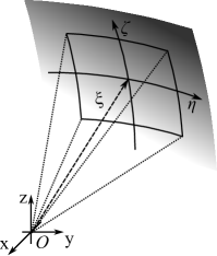
(c) Radial coordinate $\xi$ emanating from the scaling center $O$ to the boundary of the volume element

Figure 2: Scaled boundary coordinates $\xi$, $\eta$ and $\zeta$

In the scaled boundary coordinates $\left(\xi,\eta,\zeta\right)$, a point $\left(\hat{x},\hat{y},\hat{z}\right)$ inside the domain can be defined as

$$\hat{x}\!\left(\xi,\eta,\zeta\right) =\xi x\!\left(\eta,\zeta\right)=\xi\mathrm{\mathbf{N}}\!\left(\eta,\zeta\right)\mathrm{\mathbf{x}},$$ (1a)

$$\hat{y}\!\left(\xi,\eta,\zeta\right) =\xi y\!\left(\eta,\zeta\right)=\xi\mathrm{\mathbf{N}}\!\left(\eta,\zeta\right)\mathrm{\mathbf{y}},$$ (1b)

$$\hat{z}\!\left(\xi,\eta,\zeta\right) =\xi z\!\left(\eta,\zeta\right)=\xi\mathrm{\mathbf{N}}\!\left(\eta,\zeta\right)\mathrm{\mathbf{z}},$$ (1c)

where $\mathbf{x},\mathbf{y},\mathbf{z}$ are the nodal coordinate vectors of the surface element in Cartesian coordinates. The corresponding Jacobian matrix on the boundary $\left(\xi=1\right)$ is

$$\mathrm{\mathbf{J}}\!\left(\eta,\zeta\right)=\left[\begin{array}[]{ccc}x\!\left(\eta,\zeta\right)&y\!\left(\eta,\zeta\right)&z\!\left(\eta,\zeta\right)\\ x\!\left(\eta,\zeta\right)_{,\eta}&y\!\left(\eta,\zeta\right)_{,\eta}&z\!\left(\eta,\zeta\right)_{,\eta}\\ x\!\left(\eta,\zeta\right)_{,\zeta}&y\!\left(\eta,\zeta\right)_{,\zeta}&z\!\left(\eta,\zeta\right)_{,\zeta}\end{array}\right].$$ (2)

The unknown displacement functions $\mathrm{\mathbf{u}}\!\left(\xi\right)$ are introduced on the radial lines connecting the scaling center and the boundary nodes

$$\mathrm{\mathbf{u}}\!\left(\xi\right)=\underset{e}{\sum}\mathrm{\mathbf{u}}^{e}\!\left(\xi\right),$$ (3)

where $\underset{e}{\sum}$ indicates a standard finite element assembly process. Within the volume element, the displacements at a point inside a sector, formed by a surface element $e$, are interpolated as

$$\mathrm{\mathbf{u}}\!\left(\xi,\eta,\zeta\right)=\mathrm{\mathbf{N}}^{\mathrm{u}}\!\left(\eta,\zeta\right)\mathrm{\mathbf{u}}^{e}\!\left(\xi\right),$$ (4)

where $\mathrm{\mathbf{N}}^{\mathrm{u}}$ is the shape functions written in matrix form. In scaled boundary coordinates, the linear differential operator $\mathrm{\mathbf{L}}$ for the strain-displacement relationship is expressed as [16]

$$\mathrm{\mathbf{L}}=\mathrm{\mathbf{b}}_{\mathrm{1}}\!\left(\eta,\zeta\right)\frac{\partial}{\partial\xi}+\frac{1}{\xi}\!\left(\mathrm{\mathbf{b}}_{\mathrm{2}}\!\left(\eta,\zeta\right)\frac{\partial}{\partial\eta}+\mathrm{\mathbf{b}}_{\mathrm{3}}\!\left(\eta,\zeta\right)\frac{\partial}{\partial\zeta}\right),$$ (5)

where $\mathrm{\mathbf{b}}_{1}\!\left(\eta,\zeta\right)$, $\mathrm{\mathbf{b}}_{2}\!\left(\eta,\zeta\right)$ and $\mathrm{\mathbf{b}}_{3}\!\left(\eta,\zeta\right)$ are defined in [45].

Using Eqs. (4) and (5), the strains are expressed as

$$\mathrm{\boldsymbol{\varepsilon}}\!\left(\xi,\eta,\zeta\right)=\mathrm{\mathbf{B}}_{\mathrm{1}}\!\left(\eta,\zeta\right)\mathrm{\mathbf{u}}^{e}\!\left(\xi\right),_{\xi}+\frac{1}{\xi}\mathrm{\mathbf{B}}_{2}\!\left(\eta,\zeta\right)\mathrm{\mathbf{u}}^{e}\!\left(\xi\right),$$ (6)

with

$$\mathrm{\mathbf{B}}_{\mathrm{1}}\!\left(\eta,\zeta\right)= \mathrm{\mathbf{b}}_{\mathrm{1}}\!\left(\eta,\zeta\right)\mathrm{\mathbf{N}}^{\mathrm{u}}\!\left(\eta,\zeta\right),$$ (7a)

$$\mathrm{\mathbf{B}}_{\mathrm{2}}\!\left(\eta,\zeta\right)= \mathrm{\mathbf{b}}_{\mathrm{2}}\!\left(\eta,\zeta\right)\mathrm{\mathbf{N}}^{\mathrm{u}}\!\left(\eta,\zeta\right),_{\eta}+\mathrm{\mathbf{b}}_{\mathrm{3}}\!\left(\eta,\zeta\right)\mathrm{\mathbf{N}}^{\mathrm{u}}\!\left(\eta,\zeta\right),_{\zeta}.$$ (7b)

Assuming linear elasticity, the stresses are equal to

$$\mathrm{\boldsymbol{\sigma}}\!\left(\xi,\eta,\zeta\right)=\mathrm{\mathbf{D}}\!\left(\mathrm{\mathbf{B}}_{\mathrm{1}}\!\left(\eta,\zeta\right)\mathrm{\mathbf{u}}^{e}\!\left(\xi\right),_{\xi}+\frac{1}{\xi}\mathrm{\mathbf{B}}_{2}\!\left(\eta,\zeta\right)\mathrm{\mathbf{u}}^{e}\!\left(\xi\right)\right),$$ (8)

where $\mathrm{\mathbf{D}}$ is the elasticity matrix.

2.2 Solution of the scaled boundary finite element equation for elasto-statics

The scaled boundary finite element equation in displacements can be derived based on Galerkin’s method or the virtual work principle, which were reported in Refs. [16] and [17], respectively. For each volume element, the equation can be written as

$$\mathrm{\mathbf{E}_{0}}\xi^{2}\mathrm{\mathbf{u}}\!\left(\xi\right),_{\xi\xi}+\left(2\mathbf{E}_{0}-\mathbf{E}_{1}+\mathbf{E}_{1}^{\mathrm{T}}\right)\xi\mathrm{\mathbf{u}}\!\left(\xi\right),_{\xi}+\left(\mathbf{E}_{1}^{\mathrm{T}}-\mathrm{\mathbf{E}_{2}}\right)\mathrm{\mathbf{u}}\!\left(\xi\right)=\boldsymbol{0}.$$ (9)

The coefficient matrices $\mathbf{E}_{0}^{e}$, $\mathbf{E}_{1}^{e}$ and $\mathbf{E}_{2}^{e}$ of a surface element $e$ are obtained by

$$\mathbf{E}_{0}^{e}= \int_{e}\mathrm{\mathbf{B}_{1}^{\mathrm{T}}\mathrm{\mathbf{D}}\mathbf{B}_{1}}\mathrm{|\mathrm{\mathbf{J}}|d\eta d\zeta},$$ (10a)

$$\mathbf{E}_{1}^{e}= \int_{e}\mathrm{\mathbf{B}_{2}^{\mathrm{T}}\mathrm{\mathbf{D}}\mathbf{B}_{1}}\mathrm{|\mathrm{\mathbf{J}}|d\eta d\zeta},$$ (10b)

$$\mathbf{E}_{2}^{e}= \int_{e}\mathrm{\mathbf{B}_{2}^{\mathrm{T}}\mathrm{\mathbf{D}}\mathbf{B}_{2}}\mathrm{|\mathrm{\mathbf{J}}|d\eta d\zeta}.$$ (10c)

They are assembled to form the coefficient matrices $\mathbf{E}_{0}$, $\mathbf{E}_{1}$ and $\mathbf{E}_{2}$ of a volume element in Eq. (9) according to the element connectivity data. This procedure is identical to that known from the FEM. According to Song [49], the internal nodal forces $\mathrm{\mathbf{q}}\!\left(\xi\right)$ on a surface with a constant $\xi$ can be formulated as

$$\mathrm{\mathbf{q}}\!\left(\xi\right)=\xi\!\left(\mathbf{E}_{0}\xi\mathrm{\mathbf{u}}\!\left(\xi\right),_{\xi}+\mathbf{E}_{1}^{\mathrm{T}}\mathrm{\mathbf{u}}\!\left(\xi\right)\right).$$ (11)

The order of the differential equations in Eq. (9) can be reduced by one. The solution obtained from eigenvalue decomposition is given in the following form

$$\mathrm{\mathbf{u}}\!\left(\xi\right) =\mathbf{\mathrm{\Phi}}_{\mathrm{u1}}\xi^{\mathbf{-\boldsymbol{\lambda}}-0.5\mathrm{\mathbf{I}}}\mathbf{c_{\mathrm{1}}},$$ (12a)

$$\mathrm{\mathbf{q}}\!\left(\xi\right) =\mathbf{\mathrm{\Phi}}_{\mathrm{q1}}\xi^{-\mathbf{\boldsymbol{\lambda}}+0.5\mathrm{\mathbf{I}}}\mathbf{c_{\mathrm{1}}},$$ (12b)

where $-\boldsymbol{\lambda}$ is the eigenvalues, $\mathbf{\mathbf{\mathrm{\Phi}}_{\mathrm{u1}}}$ and $\mathbf{\mathbf{\mathrm{\Phi}}_{\mathrm{q1}}}$ are the sub-matrices of the eigenvector matrix, while $\mathbf{c}_{1}$ and $\mathbf{c}_{2}$ denote the integration constants. On the boundary $\left(\xi=1\right)$, the stiffness matrix of the volume element ($\mathrm{\mathbf{q}}\!\left(\xi=1\right)=\mathbf{K}\mathrm{\mathbf{u}}\!\left(\xi=1\right)$) is obtained by eliminating the integration constants $\mathbf{c}_{1}$ as

$$\mathbf{K}=\mathbf{\mathbf{\mathrm{\Phi}}_{\mathrm{q1}}}\mathbf{\mathbf{\mathrm{\Phi}}}_{\mathbf{\mathrm{u1}}}^{-1}.$$ (13)

In order to obtain the element mass matrix, a coefficient matrix $\mathbf{M}_{0}$ is introduced

$$\mathbf{M}_{0} =\underset{e}{\sum}\mathbf{M}_{0}^{e},$$ (14)

where the element coefficient matrix $\mathbf{M}_{0}^{e}$ is defined as

$$\mathbf{M}_{0}^{e} =\int_{e}\mathrm{\mathbf{N}}^{\mathrm{u}}\!\left(\eta,\zeta\right)^{\mathrm{T}}\rho\mathrm{\mathbf{N}}^{\mathrm{u}}\!\left(\eta,\zeta\right)|\mathrm{\mathbf{J}}|\mathrm{d}\eta\mathrm{d}\zeta.$$ (15)

An abbreviation $\mathbf{m}_{0}$ is introduced as

$$\mathbf{m}_{0} =\mathbf{\mathrm{\Phi}}_{\mathrm{u1}}^{\mathrm{T}}\mathbf{M}_{0}\mathbf{\mathrm{\Phi}}_{\mathrm{u1}}.$$ (16)

To integrate analytically along the radial direction, a matrix $\mathbf{m}$ is constructed, the components of which can be computed analytically based on the matrix $\mathbf{m}_{0}$

$$\mathrm{m}_{ij} =\int_{0}^{1}\xi^{\lambda_{i}}\mathrm{m}_{0ij}\xi^{\lambda_{j}}\xi^{2}\mathrm{d}\xi$$

$$=\frac{\mathrm{m}_{0ij}}{\lambda_{i}+\lambda_{j}+3},$$ (17)

and the consistent mass matrix $\mathbf{M}$ is written as

$$\mathbf{M} =\mathbf{\mathrm{\Phi}}_{\mathrm{u1}}^{-\mathrm{T}}\mathbf{m}\mathbf{\mathrm{\Phi}}_{\mathrm{u1}}^{-1}.$$ (18)

3 Explicit dynamics

In this section, the central difference equations for explicit dynamics are presented, including the discussion of an SBFEM-specific mass lumping technique and the application of octree cell patterns. The explicit solver is first presented in a serial version, which lays the foundation for the parallel explicit solver introduced in Section 4.

3.1 Explicit time integration

In our implementation of the central difference method (CDM), a fixed time step size is assumed for the sake of simplicity of the algorithm. However, it should be kept in mind that adaptive time-stepping techniques would also be possible. The displacement vector of all degrees of freedom (DOFs) at the $n$-th time step is referred to as $\mathbf{U}_{n}$. The velocity and acceleration vectors are the derivatives of the displacement vector with respect to time and are denoted by $\dot{\mathbf{U}}_{n}$ and $\ddot{\mathbf{U}}_{n}$, respectively. The equilibrium equation at the $n$-th time step using Newton’s second law can be written as

$$\mathbf{M}\ddot{\mathbf{U}}_{n}+\mathbf{C}\dot{\mathbf{U}}_{n}+\mathbf{R}_{n}^{\mathrm{int}}=\mathbf{R}_{n}^{\mathrm{ext}},$$ (19)

where $\mathbf{M}$ is the mass matrix, $\mathbf{C}$ denotes the damping matrix, $\mathbf{R}_{n}^{\mathrm{ext}}$ represents the external load vector, and the internal force vector for linear analyses is given as

$$\mathbf{R}_{n}^{\mathrm{int}}=\mathbf{K}\mathbf{U}_{n}.$$ (20)

Using the CDM, the derivatives of $\mathbf{U}_{n}$ can be approximated as

$$\dot{\mathbf{U}}_{n} =\frac{1}{2\Delta t}\!\left(\mathbf{U}_{n+1}-\mathbf{U}_{n-1}\right),$$ (21a)

$$\ddot{\mathbf{U}}_{n} =\frac{1}{\Delta t^{2}}\!\left(\mathbf{U}_{n+1}-2\mathbf{U}_{n}+\mathbf{U}_{n-1}\right),$$ (21b)

where $\Delta t$ denotes the time step. In the next step, we substitute Eqs. (21) into Eq. (19),

$$\frac{1}{\Delta t^{2}}\mathbf{M}\!\left(\mathbf{U}_{n+1}-2\mathbf{U}_{n}+\mathbf{U}_{n-1}\right)+\frac{1}{2\Delta t}\mathbf{C}\!\left(\mathbf{U}_{n+1}-\mathbf{U}_{n-1}\right)+\mathbf{R}_{n}^{\mathrm{int}}=\mathbf{R}_{n}^{\mathrm{ext}},$$ (22)

which can be solved for the displacement at the next time step, i.e., $\mathbf{U}_{n+1}$, expressed as

$$\left(\frac{1}{\Delta t^{2}}\mathbf{M}+\frac{1}{2\Delta t}\mathbf{C}\right)\mathbf{U}_{n+1} =\mathbf{R}_{n}^{\mathrm{ext}}-\mathbf{R}_{n}^{\mathrm{int}}+\frac{2}{\Delta t^{2}}\mathbf{M}\mathbf{U}_{n}-\!\left(\frac{1}{\Delta t^{2}}\mathbf{M}-\frac{1}{2\Delta t}\mathbf{C}\right)\mathbf{U}_{n-1}.$$ (23)

If mass-proportional damping is considered,

$$\mathbf{C}=\alpha\mathbf{M},$$ (24)

where $\alpha$ is a constant, Eq. (23) can be written as

$$\mathbf{U}_{n+1} =\frac{\Delta t^{2}\mathbf{M}^{-1}\!\left(\mathbf{R}_{n}^{\mathrm{ext}}-\mathbf{R}_{n}^{\mathrm{int}}\right)+2\mathbf{U}_{n}-\!\left(1-\frac{\alpha}{2}\Delta t\right)\mathbf{U}_{n-1}}{1+\frac{\alpha}{2}\Delta t}.$$ (25)

We observe that the displacement at the next step is only related to the displacement of the current and previous time steps. To start the procedure, a fictitious point $\mathbf{U}_{-1}$ is added, which is calculated as

$$\mathbf{U}_{-1}=\mathbf{U}_{0}-\Delta t\dot{\mathbf{U}}_{0}+\frac{\Delta t^{2}}{2}\ddot{\mathbf{U}}_{0}.$$ (26)

One important drawback of explicit methods is that they are generally only conditionally stable, which means there exists a critical time step $\Delta t_{\mathrm{cr}}$ which should not be exceeded, otherwise the results will diverge. Thus, they are often only used in high-frequency problems where a small time step size is already demanded by the physics of the problem. The exact value of $\Delta t_{\mathrm{cr}}$ involves the calculation of the maximum natural frequency of the whole structure, which is time and memory consuming. In our implementation, the stability limit is estimated by the maximum frequency on element level, i.e., the critical time step (in the CDM) is

$$\Delta t_{\mathrm{cr}}=\frac{2}{\omega_{\max}},$$ (27)

where $\omega_{\max}$ is the maximum frequency of all elements [6, 50].

3.2 Implementation using octree mesh

In this section, we introduce the mesh generation technique based on octree algorithm, which is highly complementary to the SBFEM. Unique octree cell patterns are discussed, which enables an efficient calculation of nodal force vector without the assembly of global stiffness matrix.

3.2.1 Balanced octree mesh for SBFEM

The octree algorithm is a highly-efficient hierarchical-tree based technique for mesh generation. It discretizes a problem domain into cells by recursively bisecting the cell edges until some specified stopping criteria are met [24]. An example of octree mesh in shown in Fig. 3a, in which each octree cell is modeled as a scaled boundary finite element. An octree mesh is usually balanced by limiting the length ratio between two adjacent cells to $2$ ($2:1$ rule). All the possible node locations of a balanced octree cell is indicated in Fig. 3b. There are $2^{12}=4096$ patterns in total [Chapter 9, 45].

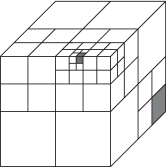
(a) A balanced octree mesh

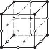
(b) A balanced octree cell indicating all possible corner ($\bullet$), mid-edge ($\circ$) and center ($+$) nodes

Figure 3: Example of balanced octree mesh and octree cell patterns [45]

When considering rotations, the faces of the cubic octree cells have only six unique node arrangements as shown in Fig. 4, depending on the number of mid-edge nodes $n_{\mathrm{h}}$ and their locations. The faces are treated as polygons in the SBFEM and discretized using rectangular and isosceles triangular elements, which are considered as high-quality elements.

(a) $n_{\mathrm{h}}=0$

(b) $n_{\mathrm{h}}=1$

(c) $n_{\mathrm{h}}=2$ adjacent edges

(d) $n_{\mathrm{h}}=2$ opposite edges

(e) $n_{\mathrm{h}}=3$

(f) $n_{\mathrm{h}}=4$

Figure 4: Discretization of the polygonal faces on the boundary of the cubic octree volume elements. The number of ’hanging nodes’ on the edges for each discretization pattern is indicated by $n_{\mathrm{h}}$.

3.2.2 Unique octree cell patterns

The 4096 patterns can be further transformed into 144 unique cases using rotation and mirroring operators. The 90 degree rotation matrices about the $x$, $y$ and $z$ axes are

$$\mathbf{T}_{\mathrm{x}}=\left[\begin{array}[]{ccc}1&0&0\\ 0&0&1\\ 0&-1&0\end{array}\right],\enskip\mathbf{T}_{\mathrm{y}}=\left[\begin{array}[]{ccc}0&0&1\\ 0&1&0\\ -1&0&0\end{array}\right],\enskip\mathbf{T}_{\mathrm{z}}=\left[\begin{array}[]{ccc}0&1&0\\ -1&0&0\\ 0&0&1\end{array}\right],$$ (28)

and the mirror matrices are

$$\mathbf{R}_{\mathrm{x}}=\left[\begin{array}[]{ccc}-1&0&0\\ 0&1&0\\ 0&0&1\end{array}\right],\enskip\mathbf{R}_{\mathrm{y}}=\left[\begin{array}[]{ccc}1&0&0\\ 0&-1&0\\ 0&0&1\end{array}\right],\enskip\mathbf{R}_{\mathrm{z}}=\left[\begin{array}[]{ccc}1&0&0\\ 0&1&0\\ 0&0&-1\end{array}\right].$$ (29)

These transformation matrices can be arranged and combined to form 48 unique transformations of an octree cell in 3D. Alternatively, the 48 transformations can be constructed directly by filling $-1$ or $1$ to each row and column of a $3\times 3$ empty matrix, i.e., there is exactly one nonzero value ($1$ or $-1$) in each row and each column. The number of transformations is equal to $3\times 2\times 1\times 2^{3}=48$. The 48 transformations involve only permutations of nodal numbers in an element, which can be easily implemented using an indexing vector. Each of the 4096 patterns can be transformed into one of the 144 unique patterns using one of the 48 transformations. All the unique octree patterns are presented in A.

The 144 patterns are determined solely by the presence or absence of mid-edge nodes, which is independent of the polyhedral element formulation selected. In our implementation, the octree meshes with triangulated boundaries are handled by the SBFEM, however it is important to note that the same approach can also be applied to other polyhedral elements with well-conditioned lumped mass matrices. The use of element patterns significantly improves computational efficiency, in terms of time and memory requirements, especially on a modern high-performance computing system.

Two sample transformations are illustrated in Fig. 5. The octree cell in Fig. 5b can be transformed into the corresponding master cell $\mathrm{c}_{1}$ in Fig. 5a by rotating 90 degrees about the $x$ axis and then rotating 90 degrees about the $z$ axis (following the right hand rule as positive rotation direction). The rotation matrix can be constructed as $\mathbf{Q}_{1}=\mathbf{T}_{\mathrm{x}}\mathbf{T}_{\mathrm{z}}$. Similarly, the octree cell in Fig. 5e can be transformed into $\mathrm{c}_{2}$ in Fig. 5d by mirroring about the $y$-$z$ plane using $\mathbf{Q}_{2}=\mathbf{R}_{\mathrm{x}}$.

(a) Octree master cell: $\mathrm{c}_{1}$

(b) Octree cell with a pattern identical to $\mathrm{c}_{1}$

$\mathbf{Q}_{1}=\left[\begin{array}[]{ccc}0&1&0\\ 0&0&1\\ 1&0&0\end{array}\right]$

(c) Transformation matrix $\mathbf{Q}_{1}=\mathbf{T}_{\mathrm{x}}\mathbf{T}_{\mathrm{z}}$

(d) Octree master cell: $\mathrm{c}_{2}$

(e) Octree cell with a pattern identical to $\mathrm{c}_{2}$

$\mathbf{Q}_{2}=\left[\begin{array}[]{ccc}-1&0&0\\ 0&1&0\\ 0&0&1\end{array}\right]$

(f) Transformation matrix $\mathbf{Q}_{2}=\mathbf{R}_{\mathrm{x}}$

Figure 5: Transformation of octree cells

When calculating the nodal force vector of an octree cell, the nodal displacement vector is transformed using the same transformation matrix $\mathbf{Q}$, which is then multiplied by the stiffness matrix of the corresponding master cell. The obtained nodal force vector must be transformed back using the inverse of transformation matrix, $\mathbf{Q}^{-1}$.

3.2.3 Implementation exploiting octree cell patterns

As an alternative to Eq. (20), $\mathbf{R}_{n}^{\mathrm{int}}$ can be calculated EBE so that the assembly of the global stiffness matrix $\mathbf{K}$ is not required.

$$\mathbf{R}_{n}^{\mathrm{int}}=\stackrel{{\scriptstyle[}}{{e}}=1]{n_{\mathrm{e}}}{\sum}\mathbf{K}_{e}\mathbf{U}_{e,n},$$ (30)

where $\sum$ represents the assembly process according to the element connectivity, $n_{\mathrm{e}}$ is the total number of elements, $\mathbf{K}_{e}$ is the element stiffness matrix of volume element $e$, and $\mathbf{U}_{e,n}$ is the nodal displacement vector of the element at the $n$-th time step.

In an octree mesh, elements of the same shape (see A) can be grouped together, and therefore, their nodal force vectors can be calculated in one step using a single matrix-multiplication. Eq. (30) can be rewritten as

$$\mathbf{R}_{n}^{\mathrm{int}}=\stackrel{{\scriptstyle[}}{{p}}=1]{n_{\mathrm{p}}}{\sum}\mathbf{K}_{p}\!\left[\begin{array}[]{cccc}\mathbf{U}_{p1}&\mathbf{U}_{p2}&\cdots&\mathbf{U}_{pk}\end{array}\right]_{n}\mathrm{diag}\!\left(\mathbf{S}\right),$$ (31)

where $n_{\mathrm{p}}$ is the number of unique patterns in the octree mesh, $\mathbf{K}_{p}$ is the stiffness matrix of a master element of pattern $p$ with unit size, $\mathbf{U}_{pi}$ is the nodal displacement vector of the $i$-th element of pattern $p$, and $\mathrm{diag}\!\left(\mathbf{S}\right)$ is a diagonal matrix containing the edge lengths of each element of pattern $p$. Each column obtained from the right-hand side will be assembled into $\mathbf{R}_{n}^{\mathrm{int}}$ using the element connectivity data. As mentioned before, the spatial discretization is based on a balanced octree mesh. This holds two important advantages: (i) all surface elements are well-shaped and (ii) for a cubic volume element only a limited number of surface patterns exist. These are the prerequisites to exploit a pre-computation technique. To this end, the stiffness and mass matrices of all master elements corresponding to the different patterns $p$ can be computed beforehand. For the pre-computation strategy, a unit size of the master element is assumed. Due to the limited surface element shapes, the stiffness and mass matrices for the master element only need to be scaled by suitable factors including information on the element size and material properties.

The stiffness matrix of an element is proportional to its Young’s modulus and edge length. On the other hand, the mass matrix of an element is proportional to the mass density and the cube of edge length. Here, we define the ratios between Young’s modulus, mass density and edge length as $\eta_{E}=\nicefrac{{E_{2}}}{{E_{1}}}$, $\eta_{\rho}=\nicefrac{{\rho_{2}}}{{\rho_{1}}}$ and $\eta_{L}=\nicefrac{{L_{2}}}{{L_{1}}}$ (see Fig. 6). Therefore, the stiffness and mass matrices, $\mathbf{K}_{2}$ and $\mathbf{M}_{2}$, of an element can be derived easily from a master element of same pattern and Poisson’s ratio as

$$\mathbf{K}_{2}=\eta_{E}\eta_{L}\mathbf{K}_{1},$$ (32a)

$$\mathbf{M}_{2}=\eta_{\rho}\eta_{L}^{3}\mathbf{M}_{1},$$ (32b)

where $\mathbf{K}_{1}$ and $\mathbf{M}_{1}$ are stiffness and mass matrices of the master element, respectively. In cases where materials with different Poisson’s ratios are present, the master element matrices have be computed for each material separately. The critical time step is estimated based on the maximum eigenfrequency of the element in Eq. (27), therefore, considering Eq. (32), $\Delta t_{\mathrm{cr}}{}_{2}$ of an element can be calculated from the known time step of the master element $\Delta t_{\mathrm{cr}}{}_{1}$,

$$\Delta t_{\mathrm{cr}}{}_{2}=\sqrt{\frac{\eta_{\rho}}{\eta_{E}}}\eta_{L}\Delta t_{\mathrm{cr}}{}_{1}.$$ (33)

(a) Master element

(b) Scaled element

Figure 6: Scaling of an octree element

3.3 Mass lumping in the SBFEM

It can be inferred from Eq. (25) that if the mass matrix $\mathbf{M}$ is given in diagonal form, it is possible to advance in time by simple matrix-vector products without the need for solving a system of linear equations. The reason for this increased efficiency lies in the trivial inversion of a diagonal matrix. In the context of the finite and spectral element methods (SEM), different mass lumping schemes have been reported and thoroughly assessed in Refs. [51, 52].

Different from the FEM and SEM, the displacement interpolations inside the scaled boundary finite elements are obtained semi-analytically, and the $x$, $y$ and $z$ displacement components are coupled. In our proposed mass lumping scheme, only those components of the mass matrix that correspond to DOFs in the same coordinate direction are summed up. The basic approach is illustrated in Fig. 7a for the DOFs related to $x$ direction. The procedure is repeated in the same fashion for the components corresponding to $y$ and $z$ directions. This method results in a block-diagonal matrix as shown in Fig. 7b, from which a diagonal mass matrix $\mathbf{M}_{\mathrm{diag}}$ is then extracted (Fig. 7c). The off-diagonal terms, which sum up to zero, are ignored. The total mass of the system is conserved in the formulation of the SBFEM. A detailed explanation and verification of this mass lumping approach has been reported by Gravenkamp et al. [47].

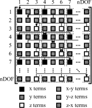
(a) Fully populated mass matrix $\mathbf{M}$

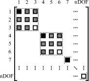
(b) Block-diagonal mass matrix

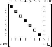
(c) Diagonal mass matrix $\mathbf{M}_{\mathrm{diag}}$

Figure 7: Lumping of the mass matrix

Due to the mass matrix $\mathbf{M}$ being available in diagonal format $\mathbf{M}_{\mathrm{diag}}$, we can re-write the expression for the displacement vector in the next time step as

$$\mathbf{U}_{n+1}=\frac{\Delta t^{2}\mathbf{M}_{\mathrm{diag}}^{-1}\!\left(\mathbf{R}_{n}^{\mathrm{ext}}-\mathbf{R}_{n}^{\mathrm{int}}\right)+2\mathbf{U}_{n}-\!\left(1-\frac{\alpha}{2}\Delta t\right)\mathbf{U}_{n-1}}{1+\frac{\alpha}{2}\Delta t}.$$ (34)

Lumping the mass matrix avoids solving a system of linear equations and as a result, each component in $\mathbf{U}_{n+1}$ can be calculated independently of the other entries. Lumped mass matrices of several octree patterns mentioned in Section 3.2.3 are presented below as ratios to the total mass of the octree cells. Poisson’s ratios are 0 and 0.3 in Fig. 8 and Fig. 9, respectively.

(a) Element with 8 nodes

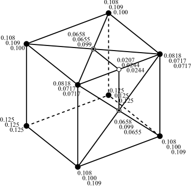
(b) Element with 11 nodes

(c) Element with 13 nodes

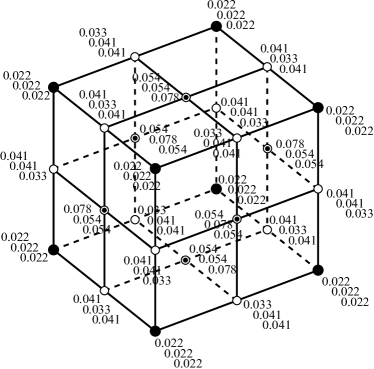
(d) Element with 26 nodes

Figure 8: Lumped mass matrices with Poisson’s ratio $\nu=0$

(a) Element with 8 nodes

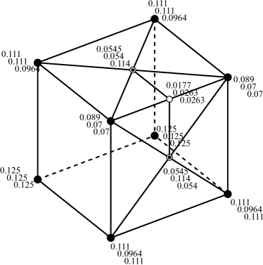
(b) Element with 11 nodes

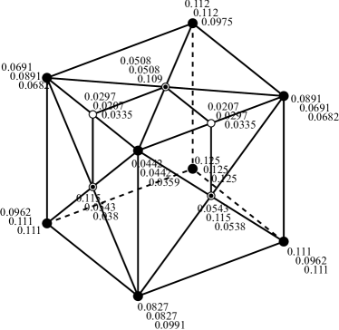
(c) Element with 13 nodes

(d) Element with 26 nodes

Figure 9: Lumped mass matrices with Poisson’s ratio $\nu=0.3$

3.4 Explicit solver in serial

Based on the previous sections, an explicit solver can be developed making use of lumped mass matrices and the unique octree patterns. The data structure of the solver is presented in Table 1. Element stiffness and mass matrices of the 144 unique octree patterns can be pre-computed and stored as $\mathbf{K}_{e}$ and $\mathbf{M}_{e}$. It is noted that if multiple materials with different Poisson’s ratios are present in the model, each material will be assigned its own $\mathbf{K}_{e}$ and $\mathbf{M}_{e}$ matrices. For each specific problem, a matrix $\mathbf{V}$ is constructed by concatenating the DOF vector of each element, which is already arranged according to the transformation matrix to the master cells. Furthermore, $n_{\mathrm{e}}$ is the number of elements, and $n_{\mathrm{dof}}$ denotes the total number of DOFs. The vector $\mathrm{\boldsymbol{\varGamma}_{D}}$ stores the DOFs which are fixed (Dirichlet boundary conditions), and $\mathrm{\boldsymbol{\varGamma}_{N}}$ is a sparse vector containing the location and magnitude of the external nodal forces (Neumann boundary conditions). $\mathrm{\mathbf{T}}$ is an integer vector indicating the element type, while $\mathrm{\mathbf{S}}$ is a vector containing the edge length of each element. The variables mentioned above are constant for each problem during the calculation. In each time step, the displacement vectors corresponding to the previous step, current step and the next step, $\mathbf{U}_{\mathrm{p}}$, $\mathbf{U}_{\mathrm{c}}$ and $\mathbf{U}_{\mathrm{n}}$, are updated accordingly. $\mathbf{R}^{\mathrm{ele}}$ is a matrix containing the nodal force vector of each element, which are grouped by element type. $\mathbf{R}^{\mathrm{int}}$ is the internal force vector which is assembled from $\mathbf{R}^{\mathrm{ele}}$, while $\mathbf{R}^{\mathrm{ext}}$ is the external force vector calculated at the time $t$. The pseudo-code of the explicit solver is presented in Algorithm 1.

Table 1: Data structure of explicit solver

	Variable	Data type	Variable type	Size	Description
Constant	$\mathbf{K}_{e}$	float	hyper-matrix	144	Element stiffness matrices of the 144 unique octree cell patterns
	$\mathbf{M}_{e}$	float	hyper-matrix	144	Diagonal mass matrices of the 144 unique octree cell patterns
Pre-compute	$\mathbf{V}$	integer	hyper-vector	$n_{\mathrm{e}}$	DOF vector of each element
	$\boldsymbol{\varGamma}_{\mathrm{D}}$	integer	vector	< $n_{\mathrm{dof}}$	Dirichlet boundary condition (the DOFs which are fixed)
	$\boldsymbol{\varGamma}_{\mathrm{N}}$	float	vector	$n_{\mathrm{dof}}$	Neumann boundary condition (the location and magnitude of external forces)
	$\mathbf{T}$	integer	vector	$n_{\mathrm{e}}$	Pattern of each element, from 1 to 144
	$\mathbf{S}$	float	vector	$n_{\mathrm{e}}$	Edge length of each element
	$\mathbf{M}_{\mathrm{diag}}$	float	matrix	$n_{\mathrm{dof}}$	Global diagonal mass matrix
Time stepping	$\mathbf{U}_{\mathrm{p}}$, $\mathbf{U}_{\mathrm{c}}$, $\mathbf{U}_{\mathrm{n}}$	float	vector	$n_{\mathrm{dof}}$	Displacement vector of previous step, current step and next step
	$\mathbf{R}^{\mathrm{ele}}$	float	hyper-vector	$n_{\mathrm{e}}$	Internal nodal force vector of each element
	$\mathbf{R}^{\mathrm{ext}}$, $\mathbf{R}^{\mathrm{int}}$	float	vector	$n_{\mathrm{dof}}$	External and internal force vectors

1:Input mesh

2:Load pre-computed master element stiffness and mass matrices $\mathbf{K}_{e}$ and $\mathbf{M}_{e}$

3:Identify element patterns $\mathrm{\mathbf{T}}$ and edge lengths $\mathbf{S}$, and link to corresponding master element

4:Assemble global $\mathbf{V}$ matrix and group based on element type

5:Assemble global diagonal mass matrix $\mathbf{M}_{\mathrm{diag}}$

6:Apply boundary conditions

7:Initialize nodal displacement vectors $\mathbf{U}_{\mathrm{p}}$, $\mathbf{U}_{\mathrm{c}}$ and $\mathbf{U}_{\mathrm{n}}$

8:for $t$ in $\left[0,T\right]$ do

9:     Initialize global nodal force vector: $\mathbf{R}^{\mathrm{int}}=\left\{\mathbf{0}\right\}$

10:     for $p=1:n_{\mathrm{p}}$ do

11:         Assemble $\mathbf{U}_{\mathrm{c}p}$ of $p$-th pattern using Eq. (31)

12:         Calculate $\mathbf{R}_{p}^{\mathrm{ele}}$ of $p$-th pattern: $\mathbf{R}_{p}^{\mathrm{ele}}=\mathbf{K}_{p}\mathbf{U}_{\mathrm{c}p}\mathrm{diag}\!\left(\mathbf{S}_{p}\right)$

13:         for $e=1:n_{\mathrm{e}}$ do

14:              Assemble the $e$-th column of $\mathbf{R}_{p}^{\mathrm{ele}}$ into $\mathbf{R}^{\mathrm{int}}$

15:         end for

16:     end for

17:     Calculate external force $\mathbf{R}_{t}^{\mathrm{ext}}$ at current time

18:     Calculate next step displacement $\mathbf{U}_{\mathrm{n}}$ using Eq. (25)

19:     $\mathbf{U}_{\mathrm{p}}=\mathbf{U}_{\mathrm{c}}$; $\mathbf{U}_{\mathrm{c}}=\mathbf{U}_{\mathrm{n}}$

20:end for

Algorithm 1 Explicit solver in serial

4 Parallel processing

Due to the fact that in explicit dynamics, the nodal force vector can be assembled in an element-wise fashion, it is natural to exploit parallel processing techniques to improve the efficiency of the solver. The basic idea is to partition the mesh into different parts and assign these parts to multiple processors. On each processor the nodal force vector is calculated, and only the interface DOFs of each part need to be synchronized. In this section, details regarding the partitioning strategy and the parallel solver are presented.

4.1 Mesh partition

Mesh partition serves a vital role in parallel processing as the quality of partition directly affects the efficiency of the solver. There are mainly two types of mesh partitioning approaches, namely node- and element-cut strategies [53]. In this work, as most of the computational effort is spent on the element processing stage, the node-cut strategy is adopted. There are two main considerations that must be taken into account in order to achieve a good partitioning of the mesh:

1. Size of the parts: An identical size of the individual parts ensures that a balanced workload is achieved, i.e., all processors complete their tasks at the same time. If that is not the case, some processors are idle, and important resources are wasted as the speedup entirely depends on the slowest processor. Although different patterns of elements require a different amount of calculation, it is reasonable to estimate the amount of work on each processor using the number of elements.

2. Interface between parts: The interface between individual parts should be as small as possible. While data communication between processors cannot be avoided in explicit dynamics because the nodal force vectors need to be synchronized in each time step, the target is to minimize the amount of data communication which is the main bottleneck in parallel processing in terms of the attainable speedup. The amount of data that needs to be transferred is measured by the number of nodes on the interface.

In order to partition a mesh, it is first converted into its dual graph. Each element in the mesh is represented by a vertex $\mathrm{v}$ in the graph, while each interface shared by two elements is represented by an edge $\mathrm{e}$ connecting two vertices. The set of vertices is denoted as $V$ and the set of edges is referred to as $E$. A typical quadtree mesh in 2D and its dual graph $G=\left\{V,E\right\}$ are depicted in Fig. 10. An optimal partition can be obtained by cutting through nodes $\left\{\mathrm{n}_{4},\mathrm{n}_{12},\mathrm{n}_{11},\mathrm{n}_{19}\right\}$ and dividing the mesh into two parts with six elements each. Cutting through $\left\{\mathrm{n}_{3},\mathrm{n}_{8},\mathrm{n}_{11},\mathrm{n}_{12},\mathrm{n}_{15},\mathrm{n}_{20}\right\}$ is sub-optimal since more nodes are involved in the cutting, and thus more results need to be communicated.

(a) A sample quadtree mesh

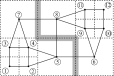
(b) Dual graph and its optimal partition (shaded line)

Figure 10: A quadtree mesh and its dual graph

However, in general, it is difficult to find the optimal partition, which is known as an NP-hard problem (non-deterministic polynomial-time hardness [54]). There are several techniques in practice that can provide a reasonably good approximation of the optimal partition, including spectral partitioners and geometric separators. The spectral partition method is based on the topology of the graph [55], while the geometric separator is based on the coordinates of the vertices [56], which can be represented by the geometric center of the elements in an octree mesh. It is noted that spectral methods are often significantly slower than geometric separators if the mesh size is large, as it involves an eigenvalue decomposition. The algorithms presented here only partition the mesh into two parts, but they can be applied recursively to obtain partitions with an integer power of two parts.

Many mesh partition packages have been developed in recent years based on these techniques [57, 58, 59]. The mesh partition package meshpart developed by Li [60] is used in this work, in which a spectral partitioner is used for examples with less than 5 million DOFs, while a geometric separator is used for all other cases.

4.2 Explicit solver in parallel

The explicit solver provided in Algorithm 1 can be easily parallelized based on the structure shown in Fig. 11. The mesh generation and mesh partition are executed on the head node (the main computer node which distributes jobs to individual processors), and the element matrices of the 144 unique master cells are stored as a static library, which is loaded every time the code runs. The mesh partition package will generate an array of size $n_{\mathrm{e}}$, which stores a flag for each element, indicating the part to which it belongs. The element DOF vectors are grouped based on this array, and they are assigned to the different processors. The displacement vectors are initialized and distributed to the processors, where each processor only stores the chunk associated with its own nodes. At each time step, the nodal force vector is calculated using Eq. (31) on each processor locally. This local version of the nodal force vector can be divided into two parts, the one corresponding to the nodes inside each part (internal DOFs) and those shared with other parts (external DOFs). The values of the latter part must be updated (corrected) by the contributions of the adjacent part(s). The values of the external nodes in the local nodal force vectors are summed and synchronized for all the processors so that the contribution from all elements connected to the interface is included. As the size of the interface is relatively small compared to the total size, this operation can be done in a relatively short time. After the updated nodal force vector is distributed to each processor, the local portion of displacement of the next step $\mathbf{U}_{n+1}$ is calculated.

Figure 11: Parallel code structure

At the beginning of the program, the octree mesh is generated and partitioned. Pre-computed stiffness and mass matrices of the master cells are imported and linked to the individual elements using corresponding transformation matrices. The vector $\mathbf{V}$ is constructed and distributed to individual processors based on the partitioning result. The initial displacement vector $\mathbf{U}_{0}$ and fictitious $\mathbf{U}_{-1}$ are calculated and distributed to processors. These steps are considered as an initialization stage, and are not included in the timing as they take constant time independent of the number of time steps. The speedup of the parallel solver is measured based on the time spent after the initialization stage, including the calculation of the nodal force vector, the synchronization between processors and the calculation of the nodal displacement vector.

A sample timing of a parallel computation using 32 processors is shown in Fig. 12. It can be observed that the speed of these processors is usually different, as well as the amount of work distributed to each processor. The light gray bar represents the time spent by each processor to calculate the nodal force vector locally, and the dark gray bar indicates the time for each processor to wait for the slower ones to finish their job and communicate the results. The black bar represents the time required to calculate the displacement vector for the next time step once the overall nodal force is obtained.

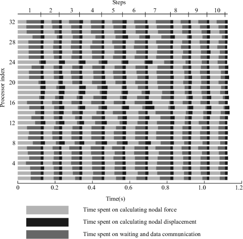
Figure 12: A sample of time distribution of parallel processing

In parallel computing, the accurate measurement of computational time is difficult since different processors usually start working at different time. Here we use the reasonable assumption that all processors commence the calculation when the first (earliest) processor starts, and all of them finish when the slowest processor completes the assigned task. In the numerical examples, the average calculation time for all processors (including light gray and black bars in Fig. 12) and communication and waiting time (dark gray bars) are used to indicate the performance of the proposed method.

5 Numerical examples

In this section, five numerical examples are presented to verify the proposed procedure and to demonstrate the attainable speedup of the novel parallel explicit solver with increasing number of computing cores. The efficiency $\eta$ of the parallel computation is measured by the ratio of the speedup and the number of cores (strong scaling). The different transient amplitude functions that are used for our numerical examples to describe the time-dependent excitations are depicted in Fig. 13. Depending on the problem, we choose either a Ricker wavelet (see Fig. 13a), a triangular pulse (see Fig. 13c), or a sine-burst signal (see Fig. 13e). The analytical form of the Ricker wavelet in the time domain is

$$P\!\left(t\right)=\!\left(1-\!\left(\frac{t-t_{1}}{t_{1}/5}\right)^{2}\right)\exp\!\left(-\frac{1}{2}\!\left(\frac{t-t_{1}}{t_{1}/5}\right)^{2}\right)P_{0},$$ (35)

where $P_{0}$ is the maximum load. The triangular impact load is expressed as

$$P\!\left(t\right)=\!\begin{cases}\!\left(1-\!\left|\frac{t}{t_{1}}-1\right|\right)P_{0}&\textrm{if }0\leq t\leq 2t_{1}\\ 0&\textrm{if }t>2t_{1}\end{cases},$$ (36)

while the sine-burst (sine excitation modulated by a Hann window) is expressed as

$$P\!\left(t\right)=\!\begin{cases}\sin\!\left(\frac{2\pi nt}{t_{1}}\right)\sin^{2}\!\left(\frac{\pi t}{t_{1}}\right)P_{0}&\textrm{if }0\leq t\leq t_{1}\\ 0&\textrm{if }t>t_{1}\end{cases},$$ (37)

where $n$ is the number of cycles. The central frequency $f_{\mathrm{m}}$ is calculated as

$$f_{\mathrm{m}}=\frac{n}{t_{1}}.$$ (38)

To obtain the frequency spectrum of the given excitation functions we apply the Fourier transform. The frequency spectrum of the Ricker wavelet is depicted in Fig. 13b and can be expressed as

$$A\!\left(f\right)=\!\left(\dfrac{2}{\sqrt{\pi}}\right)\!\left(\dfrac{f}{f_{m}}\right)^{2}\exp\!\left(-\!\left(\dfrac{f}{f_{m}}\right)^{2}\right),$$ (39)

where the central frequency $f_{\mathrm{m}}$ is

$$f_{\mathrm{m}}=\frac{5}{\sqrt{2}\pi t_{1}}.$$ (40)

Similarly, the amplitude spectrum of the Fourier transform of the triangular pulse is shown in Fig 13d and can be written as

$$A\!\left(f\right)=\!\left(\frac{\sin\!\left(\pi ft_{1}\right)}{\pi ft_{1}}\right)^{2},$$ (41)

A critical frequency $f_{1}$ is identified such that the area under the curve on the left of $f_{1}$ is equal to a certain percentage of the total area, e.g., $95\%$. This approach ensures that most of the energy content of the signal is accounted for. For a Ricker wavelet, $f_{1}$ is approximately $2.2/t_{1}$, while in the case of triangular impact $f_{1}$ is $1.8/t_{1}$. For the sine-burst excitation, $f_{1}$ is identified corresponding to $85\%$ of the area, which is $5.8/t_{1}$ when $n=5$. The determined critical frequency is an important parameter that is closely related to the required spatial discretization. Depending on the value of $f_{1}$ the wave velocities of the propagating modes are calculated from which the number of nodes per wavelength is derived.

(a) Load history of a Ricker wavelet

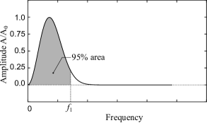
(b) Spectrum of a Ricker wavelet

(c) Load history of a triangular pulsed

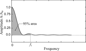
(d) Spectrum of a triangular pulse

(e) Load history of a sine-burst signal

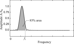
(f) Spectrum of a sine-burst signal

Figure 13: Dynamic loading for the examples

In infinite elastic media the only propagating waves are bulk waves which can be distinguished in two types, i.e., dilatational/pressure/primary and shear/secondary waves. The dilatational wave velocity $v_{\mathrm{P}}$ and shear wave velocity $v_{\mathrm{S}}$ for an isotropic, homogeneous, linear-elastic medium are calculated as

$$v_{\mathrm{P}} =\sqrt{\frac{E\!\left(1-\nu\right)}{\rho\!\left(1+\nu\right)\!\left(1-2\nu\right)}},$$ (42a)

$$v_{\mathrm{S}} =\sqrt{\frac{E}{2\rho\!\left(1+\nu\right)}},$$ (42b)

where $E$ is Young’s modulus, $\nu$ denotes Poisson’s ratio, and $\rho$ stands for the mass density of the material. Therefore, the minimum dilatational wavelength $L_{\mathrm{P}}$ and shear wavelength $L_{\mathrm{S}}$ considered in the structure are

$$L_{\mathrm{P}} =\frac{v_{\mathrm{P}}}{f_{1}},$$ (43a)

$$L_{\mathrm{S}} =\frac{v_{\mathrm{S}}}{f_{1}}.$$ (43b)

A common assumption on the spatial discretization is that the maximum element size in the mesh should be limited to have at least 10 (linear) finite elements per wavelength. This is a bare minimum which will result in deviations of more than 1% compared to a reference solution. Therefore, Willberg et al. [61] and Gravenkamp [62] recommend roughly 30 nodes per wavelength when using linear shape function in numerical methods for wave propagation analysis.

The in-house solver is written in Python 3.7, while the inter-processor communication is implemented using MPI4Py [63, 64, 65], which provides bindings for the Message Passing Interface (MPI) standard with OpenMPI (4.0.2) as the back end. The distributed computing environment used in this research is the supercomputer Gadi maintained by the national computing infrastructure (NCI) in Canberra (Australia). A typical compute node on Gadi has two sockets, each equipped with a 24-core Intel Xeon Scalable ‘Cascade Lake’ processor and connected to $190\,\mathrm{GB}$ RAM. The compute nodes and the storage systems are connected through a high-speed network with a data transfer rate of up to $200\,\mathrm{Gbps}$. In order to maximize the parallel performance, the MPI processes are mapped by sockets within each compute node, which provides an optimal achievable memory bandwidth to each MPI process on both sockets [66]. For multi-node computations, the MPI processes are evenly distributed among the compute nodes to fully exploit the computational capability of Gadi.

5.1 Eigenfrequencies of a cube

In the first example, we verify the lumped mass matrix by investigating the eigenfrequencies of a cube with a Young’s modulus of $E=1000\,\mathrm{Pa}$ and a Poisson’s ratio of $\nu=0.3$, while the mass density of the cube is chosen as $\rho=1\,\nicefrac{\mathrm{kg}}{\mathrm{m^{3}}}$. The edge length of the cube is $L=8\,\mathrm{m}$. The displacements perpendicular to the surfaces are constrained as shown in 2D in Fig. 14.

Figure 14: Geometry and boundary conditions of the cube

Three types of meshes are generated based on three typical octree patterns depicted in Fig. 15. Note that in the coarsest mesh the edge length of an element is $1\,\mathrm{m}$. The eigenfrequencies based on these meshes using either a consistent mass matrix (CMM) or a lumped mass matrix (LMM) are calculated, as well as the FEM result calculated using commercial software ABAQUS with type 1 mesh. More detailed investigations regarding the use of LMMs in the framework of the SBFEM are discussed in Ref. [47]. A convergence study of all element types is performed, and the $L_{2}$ norm of the relative error $e$ in the first 100 frequencies is presented in Fig. 16. The error $e$ is calculated as

$$e=\sqrt{\frac{\stackrel{{\scriptstyle[}}{{i}}=1]{100}{\sum}\left(\omega_{i}^{\mathrm{num}}-\omega_{i}^{\mathrm{ref}}\right)^{2}}{\stackrel{{\scriptstyle[}}{{i}}=1]{100}{\sum}\left(\omega_{i}^{\mathrm{ref}}\right)^{2}},}$$ (44)

where $\omega_{i}^{\mathrm{num}}$ is the numerical solution of the $i$-th eigenfrequency, and $\omega_{i}^{\mathrm{ref}}$ is the analytical (reference) solution. The analytical solution is given in the form

$$\omega^{\mathrm{ref}}=\sqrt{\frac{E\pi^{2}}{\rho\left(1-\nu^{2}\right)L^{2}}\!\left(l^{2}+m^{2}+n^{2}\right)\gamma},$$ (45)

where $l$, $m$ and $n$ are non-negative integers, and the parameter $\gamma$ is defined as

$$\gamma=\!\begin{cases}1&\textrm{if two of $\left\{l,m,n\right\}$ are 0 }\\ \!\left\{1,\frac{1-\nu}{2}\right\}&\textrm{if one of $\left\{l,m,n\right\}$ is 0}\\ \!\left\{1,\frac{1-\nu}{2},\frac{1-\nu}{2}\right\}&\textrm{if none of $\left\{l,m,n\right\}$ is 0}\end{cases},$$ (46)

Note that if all of $\left\{l,m,n\right\}$ are zeros, there is no solution to the equation.

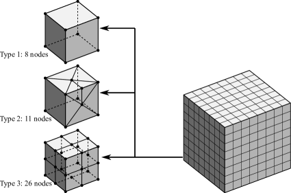
Figure 15: Three types of meshes of the cube

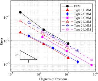
Figure 16: Relative error of first 100 eigenfrequencies calculated from different types of meshes using different methods

The numerical results depicted in Fig. 16 highlight that with the proposed approach, an optimal convergence rate (2/3) is achieved independent of using either an LMM- or CMM-based formulation in the SBFEM or the FEM formulation. Furthermore, we observe that the different octree pattern types have no influence on the slope of the curves. Although the same rates of convergence are attainable, we have to note that in general the CMM-based approach yields slightly more accurate results for the same number of DOFs, and the FEM solution is less accurate than both LMM- or CMM-based approach, which results in an offset of the error curves. This difference is, however, of no concern for the following discussions as optimal convergence is still observed.

5.2 Wave propagation in a beam

In the second example, a cantilever beam is investigated, whose dimensions are $16\,\mathrm{m}\times 1\,\mathrm{m}\times 1\,\mathrm{m}$. Its material properties are: Young’s modulus $E=10\,\mathrm{kPa}$, Poisson’s ratio $\nu=0$, and mass density $\rho=1\,\nicefrac{\mathrm{kg}}{\mathrm{m^{3}}}$. The beam is fixed on one end, and a uniform pressure load is applied on the other end, which follows the Ricker wavelet depicted in Fig. 13a with the parameters $t_{1}=15\,\mathrm{ms}$ and $P_{0}=1\,\mathrm{Pa}$. Therefore, the maximum frequency of interest $f_{1}$ is $150\,\mathrm{Hz}$. The dilatational wave speed, calculated using Eq. (42), is $100\,\nicefrac{\mathrm{m}}{\mathrm{s}}$, and the wavelength in the beam is $0.67\,\mathrm{m}$ according to Eq. (43). This problem is equivalent to a 1D wave propagation problem; therefore, Duhamel’s integral is applied to obtain a reference solution for the displacement response, the details of which can be found in Ref. [47].

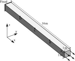
Figure 17: Geometry and boundary conditions of the beam

Again, three types of meshes are generated based on three typical octree patterns as shown in Fig. 18, and the convergence behavior is examined. In the coarsest group of meshes, the element size is set to $0.0625\,\mathrm{m}$; as a result, there are approximately 10 elements in a wavelength. The time steps in the three coarsest meshes are $0.5897\,\mathrm{ms}$, $0.3141\,\mathrm{ms}$ and $0.3380\,\mathrm{ms}$, which guarantees there are at least 10 time steps during a period of the highest frequency. The displacement and acceleration history of four selected points are plotted in Fig. 19. The $L_{2}$ norm of the error of the selected points at all time steps is calculated, and the convergence curves of these meshes are presented in Fig. 20.

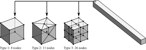
Figure 18: Three types of meshes of the beam

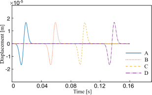
(a) Displacement history of four selected points

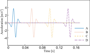
(b) Acceleration history of four selected points

Figure 19: Displacement and acceleration histories of four selected points on the beam

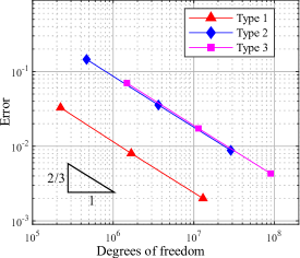
(a) Convergence curve of displacement

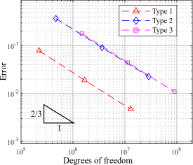
(b) Convergence curve of acceleration

Figure 20: Convergence curves of different types of meshes

As in the modal analysis example of the previous section, we observe that the theoretical rates of convergence for both displacement and acceleration are recovered by our approach, independent of the chosen mesh type. These results confirm the correctness of the implementation and provide confidence in the performance of our method. Thus, more complex examples that are of practical interest are tackled in the following sections.

5.3 Multi-story building induced ground vibration

To further verify the proposed technique and evaluate its computational performance, the ground vibration induced by a dynamic load applied to a multi-story building is analyzed. The multi-story building and the adjacent ground are depicted in Fig. 21. The building consists of columns, beams, slabs and a foundation with a basement, and the dimensions are illustrated in Fig. 22.

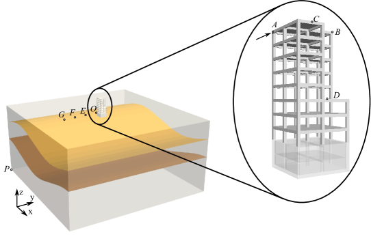
Figure 21: Geometry of the frame and ground

Figure 22: Dimension of the frame (Unit: mm)

The material properties of the frame are: Young’s modulus $E=17\,\mathrm{GPa}$, Poisson’s ratio $\nu=0.2$ and mass density $\rho=2400\,\nicefrac{\mathrm{kg}}{\mathrm{m^{3}}}$. The dilatational wave speed is equal to $2805\,\nicefrac{\mathrm{m}}{\mathrm{s}}$, and the shear wave speed is $1718\,\nicefrac{\mathrm{m}}{\mathrm{s}}$. A region of $400\,\mathrm{m}\times 400\,\mathrm{m}\times 200\,\mathrm{m}$ of the ground adjacent to the building is included in the model. The coordinates of point $P$ depicted in Fig. 21 are $\left(-183\,\mathrm{m},-187\,\mathrm{m},-200\,\mathrm{m}\right)$, and the origin of the coordinate system is denoted as $O$. The ground is made of three layers, and the shapes of these interfaces between the individual layers are defined as (unit: m)

$$z_{12} =-60+20\times\sin\!\left(\frac{x+183}{200}\pi\right),$$ (47a)

$$z_{23} =-130+20\times\cos\!\left(\frac{x+183}{200}\pi\right).$$ (47b)

From the top to the bottom layers, the Young’s moduli are equal to $0.5\,\mathrm{GPa}$, $0.8\,\mathrm{GPa}$ and $1\,\mathrm{GPa}$, respectively. All three layers have the same Poisson’s ratio of $\nu=0.2$ and mass density of $\rho=2400\,\nicefrac{\mathrm{kg}}{\mathrm{m^{3}}}$. The corresponding dilatational wave velocities are equal to $481\,\nicefrac{\mathrm{m}}{\mathrm{s}}$, $609\,\nicefrac{\mathrm{m}}{\mathrm{s}}$ and $680\,\nicefrac{\mathrm{m}}{\mathrm{s}}$, and the shear wave velocities are $295\,\nicefrac{\mathrm{m}}{\mathrm{s}}$, $373\,\nicefrac{\mathrm{m}}{\mathrm{s}}$ and $417\,\nicefrac{\mathrm{m}}{\mathrm{s}}$.

An area of $1\,\mathrm{m^{2}}$ at the side of the top of the building ($2.5\,\mathrm{m}\leq x\leq 3.5\,\mathrm{m}$, $y=2.5\,\mathrm{m}$ and $39\,\mathrm{m}\leq z\leq 40\,\mathrm{m}$), indicated by region $A$ in Fig. 21, is subjected to an impact load described by Fig. 13c with the peak pressure of $P_{0}=10^{7}\,\mathrm{Pa}$. The half duration of the impact is $t_{1}=250\,\mathrm{ms}$, and the maximum frequency of interest is $8\,\mathrm{Hz}$.

A reference solution is obtained from a convergence study using the commercial finite element package ABAQUS. To limit the size of the problem, only the building including its foundation with basement is modeled. The displacements perpendicular to the side faces below the ground level and the bottom of the basement are constrained. The displacement and acceleration responses at Points $B$, $C$ and $D$ ($B\!\left(2.5\,\mathrm{m},22.5\,\mathrm{m},40\,\mathrm{m}\right)$, corner of the building; $C\!\left(22.5\,\mathrm{m},7.5\,\mathrm{m},40\,\mathrm{m}\right)$, middle of a beam; $D\!\left(17\,\mathrm{m},17\,\mathrm{m},15\,\mathrm{m}\right)$, center of a slab) indicated in Fig. 21 are considered. A series of analyses using uniform meshes of hexahedral elements (C3D8) are performed. From the results of the convergence study we can infer that an acceptable accuracy is obtained for meshes with an element size of $0.0625\,\mathrm{m}$. Such a mesh contains 9,242,624 elements and 32,186,598 DOFs.

Generating a non-uniform hexahedral mesh for an efficient simulation of wave propagation in the complete system including both building and ground requires considerable human interventions. To compare with the present technique using octree meshes that are generated fully automatically (shown as a part of Fig. 23), non-structured tetrahedral meshes are used in ABAQUS. Both types of meshes are generated according to specified element sizes. Using the building model and the reference solution, we identify a tetrahedral mesh and an octree mesh that yield a similar level of accuracy in the displacement and acceleration response histories as plotted in Fig. 24. The minimum and maximum element sizes are $0.0625\,\mathrm{m}$ and $0.25\,\mathrm{m}$, respectively. Using our SBFEM-based code in conjunction with an octree mesh, the number of elements in the building model is 6,018,480 and therefore, the number of DOFs is 25,789,146. On the other hand, the tetrahedral mesh generated in ABAQUS has a minimum element size of $0.05\,\mathrm{m}$ while the maximum element size is $0.25\,\mathrm{m}$. Hence, there are 27,274,592 elements and 21,632,154 DOFs in the mesh.

To model the ground, both the tetrahedral and octree meshes are generated with a maximum element size of $4\,\mathrm{m}$, which is about 1/10 of the shear wavelength of $36.9\,\mathrm{m}$ in the top layer at the maximum frequency of interest. There are 7,339,939 elements and 30,482,412 DOFs in the octree mesh of the whole system (Fig. 23), while there are 38,847,472 elements and 26,192,571 DOFs in the tetrahedral mesh. The time step used in this example is $\Delta t=0.018\,\mathrm{ms}$ which was estimated using Eq. (27). Damping coefficient in Eq. (24) is chosen as $\alpha=0.1$. A total duration of $1\,\mathrm{s}$ is analyzed with 55,556 steps.

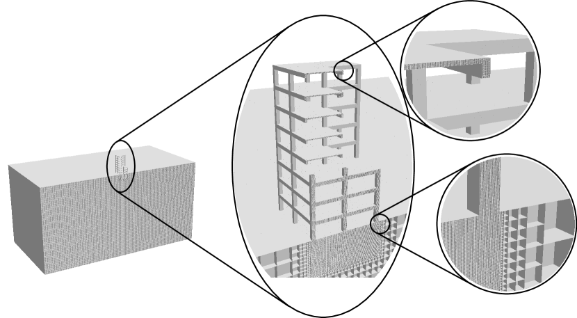
Figure 23: Octree mesh of the frame and ground

Three points $E\!\left(0\,\mathrm{m},-30\,\mathrm{m},0\,\mathrm{m}\right)$, $F\!\left(0\,\mathrm{m},-60\,\mathrm{m},0\,\mathrm{m}\right)$ and $G\!\left(0\,\mathrm{m},-90\,\mathrm{m},0\,\mathrm{m}\right)$ indicated in Fig. 21 and located at a certain distance from the building are selected for comparison purposes. The corresponding displacement and acceleration response histories are plotted in Fig. 25. It is observed that similar results are obtained with ABAQUS using the tetrahedral mesh and with our in-house code utilizing the octree mesh. The process of wave propagation in the ground is illustrated in Fig. 26 at four selected time instances.

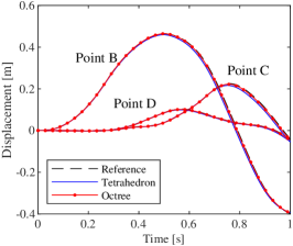
(a) Displacement of points $B$, $C$ and $D$

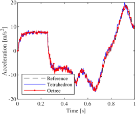
(b) Acceleration of points $B$

(c) Acceleration of points $C$

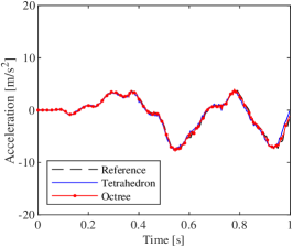
(d) Acceleration of points $D$

Figure 24: The displacement and acceleration history of the building using our in-house code and ABAQUS

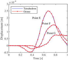
(a) Displacement at points $E$, $F$ and $G$

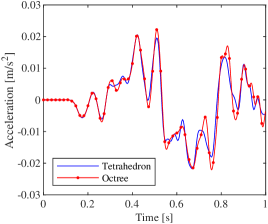
(b) Acceleration at point $E$

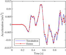
(c) Acceleration at point $F$

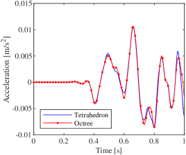
(d) Acceleration at point $G$

Figure 25: Displacement and acceleration history at selected points on the ground surface obtained with in-house code and ABAQUS

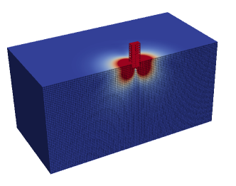
(a) $t=0.15\,\mathrm{s}$

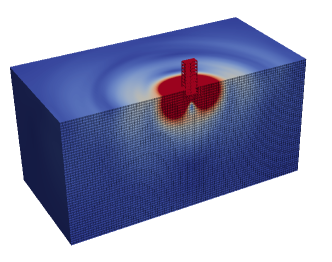
(b) $t=0.3\,\mathrm{s}$

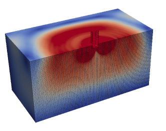
(c) $t=0.45\,\mathrm{s}$

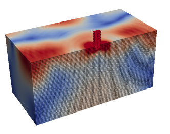
(d) $t=0.6\,\mathrm{s}$

Figure 26: Contour of displacement magnitude in the ground at various time instances $t$

Since the computational time increases linearly with the number of steps of time integration, the CPU time required to complete 1000 steps is selected in measuring the computational performance. This choice is made to facilitate the evaluation of the speedup of parallel computing, starting from a small number of cores. The computational times taken by the in-house code implementing the present technique and by ABAQUS are listed in Table 2 and are plotted in a log-log scale in Fig. 27a. To limit the wall-clock time required by the ABAQUS analyses, we opt for using four or more computer cores. It is observed that our in-house code is significantly faster than the commercial software ABAQUS when using a tetrahedral mesh to obtain an accuracy similar to our octree-based solver. The speedup compared to a single core simulation and the efficiency of the proposed method are shown in Fig. 27b.

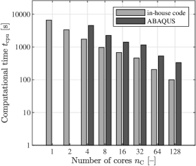
(a) Computational time taken by ABAQUS and the in-house code with different number of cores

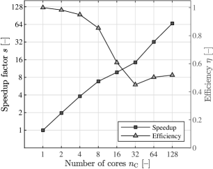
(b) Speedup and efficiency of in-house code at different number of cores

Figure 27: Comparison of computational time of the in-house code using octree mesh and ABAQUS using tetrahedral mesh

Table 2: Computational time, speedup and efficiency of in-house code and ABAQUS

$N_{\mathrm{cores}}$	ABAQUS	in-house code					Ratio $t_{\mathrm{T\textrm{-ABAQUS}}}/t_{\mathrm{T\textrm{-in-house}}}$
	$t_{\mathrm{T}}$ [s]	$t_{\mathrm{C}}$ [s]	$t_{\mathrm{W}}$ [s]	$t_{\mathrm{T}}$ [s]	$s$	$\eta$
1	-	6565.47	-	6566.12	1.00	1.00	-
2	-	3078.62	155.46	3234.37	2.03	1.02	-
4	4550	1651.08	92.94	1744.20	3.76	0.94	2.61
8	2264	894.91	58.47	953.49	6.89	0.86	2.37
16	1407	634.49	45.90	680.48	9.65	0.60	2.07
32	1154	355.03	94.84	449.92	14.59	0.46	2.56
64	534	141.43	63.28	204.73	32.07	0.50	2.61
128	334	52.18	41.66	93.85	69.97	0.55	3.56
$t_{\mathrm{C}}$: Calculation time
$t_{\mathrm{W}}$: Waiting and communication time
$t_{\mathrm{T}}$: Total time
$s$: Speedup factor
$\eta$: Efficiency

We observe that with an increasing number of cores the computational time is significantly reduced in both our in-house research code and in ABAQUS. Additionally, it is noted that the proposed explicit solver outperforms ABAQUS by a factor of at least two, meaning that for this example only half of the computational time or less is required (Table 2). The parallel efficiency for the frame example stays in a reasonable range around 50% for 128 cores. For 128 cores, only around 230,000 DOFs are distributed to each core, which might be one source for the decreasing efficiency with an increasing number of cores. The results depicted in Fig. 27b indicate that it is preferable to partition the mesh such that more than one million DOFs are distributed to each core. This is related to a more favorable ratio between time spent on calculating nodal forces and displacements in contrast to the communication and waiting time; therefore, the computational resources can be used more efficiently.

5.4 Mountainous region

In this example, wave propagation in a mountainous region of size $21.8\,\mathrm{km}\times 18.0\,\mathrm{km}$ is investigated as an indication of the practical applicability of the proposed parallel explicit solver. The location of the region is shown in a satellite image from Google Maps in Fig. 28a, while the terrain information (Fig. 28b) and the STL model (Fig. 28c) are generated using the online service Terrain2STL at http://jthatch.com/Terrain2STL/ [67]. For illustration purposes, the model is assumed to be homogeneous with a Young’s modulus $E=55\,\mathrm{GPa}$, Poisson’s ratio $\nu=0.2$ and mass density $\rho=2400\,\nicefrac{\mathrm{kg}}{\mathrm{m^{3}}}$. The dilatational wave speed is $5046\,\nicefrac{\mathrm{m}}{\mathrm{s}}$, while the shear wave speed is $3090\,\nicefrac{\mathrm{m}}{\mathrm{s}}$. The boundary conditions of the model are shown in Fig. 29, where the displacements perpendicular to the side faces and the bottom are constrained. An excitation in the form of a Ricker wavelet (Fig. 13a) with $t_{1}=0.5\,{\textstyle\mathrm{s}}$ and $P_{0}=1.157\times 10^{15}\,\mathrm{N}$ is applied at the center of the bottom of the model (point $A$) in the $y$ direction. The maximum frequency of interest is $5\,\mathrm{Hz}$, therefore, the wavelength of the shear wave is $618\,\mathrm{m}$.

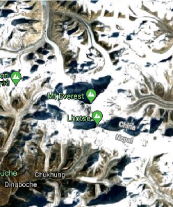
(a) Satellite image

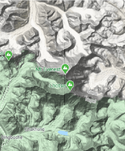
(b) Terrain

(c) STL model

Figure 28: Geometry of the mountainous region

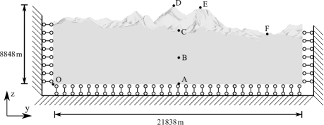
Figure 29: Boundary condition and dimensions of the mountainous region

An octree mesh is generated with a maximum element size of $68.125\,\mathrm{m}$ and a minimum element size of $8.516\,\mathrm{m}.$ Hence, the mesh consists of 7,608,933 elements and 32,052,075 DOFs. The mesh is partitioned using the algorithm proposed in Ref. [56]. The obtained mesh partitioning is depicted in B. The time step is chosen as $\Delta t=1.38\,\mathrm{ms}$. The response is analyzed for a duration of $10\,\mathrm{s}$ using 7246 time steps. The results at the points $B\!\left(9000\,\mathrm{m},10000\,\mathrm{m},4000\,\mathrm{m}\right)$, $C\!\left(7848\,\mathrm{m},11090\,\mathrm{m},5460\,\mathrm{m}\right)$, $D\!\left(11431\,\mathrm{m},11772\,\mathrm{m},7848\,\mathrm{m}\right)$, $E\!\left(11772\,\mathrm{m},9042\,\mathrm{m},7336\,\mathrm{m}\right)$ and $F\!\left(9895\,\mathrm{m},4095\,\mathrm{m},4265\,\mathrm{m}\right)$ are selected to evaluate the results and to illustrate the time-dependent displacements. The origin of the coordinate system is point $O$ in Fig. 29. The displacement and acceleration in $y$ direction of these points are plotted against time in Fig. 30. The contour of displacement magnitude at four time instances are presented in Fig. 31, illustrating the wave propagation process.

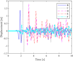
(a) Displacements

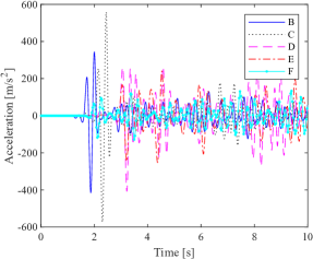
(b) Accelerations

Figure 30: Displacements and accelerations in $y$ direction at five selected points in the mountainous region model

(a) $t=0.5\,\mathrm{s}$

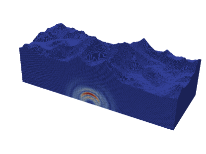
(b) $t=1\,\mathrm{s}$

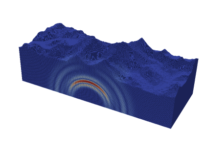
(c) $t=1.5\,\mathrm{s}$

(d) $t=2\,\mathrm{s}$

Figure 31: Contour of displacement magnitude of the mountain region model at four selected time instances $t$

The computational time and speedup for 1000 steps using different numbers of cores are compared in Fig. 32 and Table 3. The presented results in terms of the speedup factor and the parallel efficiency are in good agreement with those reported for the frame example in Section 5.3. We again observe that the efficiency of the parallel explicit solver decreases when fewer DOFs are distributed to each core. However, in this example, a higher parallel efficiency of roughly 60% is achieved due to the shape of the model, which is more regular and allows for a better partitioning.

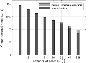
(a) Computational time

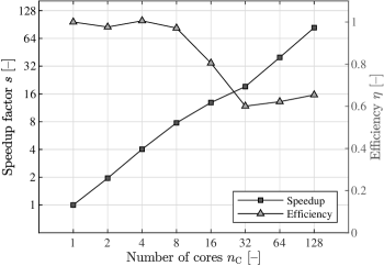
(b) Speedup and efficiency

Figure 32: Computational time, speedup and efficiency of the mountainous region simulation using different numbers of cores

Table 3: Computational time, speedup and efficiency of the mountainous region

$N_{\mathrm{cores}}$	$t_{\mathrm{C}}$ [s]	$t_{\mathrm{W}}$ [s]	$t_{\mathrm{T}}$ [s]	$s$	$\eta$
1	7273.36	-	7273.94	1.00	1.00
2	3650.19	46.03	3696.50	1.97	0.99
4	1788.73	36.26	1825.15	3.99	1.00
8	868.96	74.28	943.34	7.71	0.96
16	504.91	65.58	570.55	12.7	0.79
32	280.71	101.89	382.62	19.0	0.59
64	136.02	47.31	183.34	39.7	0.62
128	51.72	34.58	86.30	84.3	0.66
$t_{\mathrm{C}}$: Calculation time
$t_{\mathrm{W}}$: Waiting and communication time
$t_{\mathrm{T}}$: Total time
$s$: Speedup factor
$\eta$: Efficiency

5.5 Sandwich panel

In the last example, a sandwich panel with two steel cover sheets and a foam-like aluminum core is modeled. The digital image, shown in Fig. 33a, is obtained by X-ray CT scans. The size of the panel is $288\,\mathrm{mm}\times 288\,\mathrm{mm}\times 57.6\,\mathrm{mm}$, while the thickness of the cover sheet is $4.8\,\mathrm{mm}$. Young’s modulus, Poisson’s ratio and the mass density of aluminum are $E_{\mathrm{a}}=70\,\mathrm{GPa}$, $\nu_{\mathrm{a}}=0.3$ and $\rho_{\mathrm{a}}=2700\,\nicefrac{\mathrm{kg}}{\mathrm{m^{3}}}$, while the corresponding material parameters of steel are taken as $E_{\mathrm{s}}=210\,\mathrm{GPa}$, $\nu_{\mathrm{s}}=0.3$ and $\rho_{\mathrm{s}}=8050\,\nicefrac{\mathrm{kg}}{\mathrm{m^{3}}}$. An octree mesh is generated with a maximum element size of $0.96\,\mathrm{mm}$ and a minimum element size of $0.24\,\mathrm{mm}$, as shown in Fig. 33b. The mesh consists of 13,520,194 elements and 66,645,588 DOFs (for comparison, a uniform voxel based mesh would contain 89,862,518 elements and 288,049,833 DOFs). In order to test our approach for massively parallel computing of large-scale wave propagation problems and examine the increase of CPU time with the problem-size, we mirror the panel in the $x$ and $y$ directions twice. Hence, the edge length of the panel becomes $576\,\mathrm{mm}$ ($2\times 2$ panel, Fig. 34a) and $1152\,\mathrm{mm}$ ($4\times 4$ panel, Fig. 34b), respectively. In the $2\times 2$ panel, there are 54,080,776 elements and 266,295,885 DOFs, and in the $4\times 4$ panel the number of elements is 216,323,104, and the number of DOFs is 1,064,602,902.

In the simulation, we fix the displacement DOFs of the side faces at $x=0$ and $y=0$ in orthogonal direction, as indicated in Fig. 35. Additionally, Neumann boundary conditions are applied to approximate the wave excitation that is usually achieved by means of piezoelectric transducers being attached to the plate. To this end, two distributed line loads, $P_{\mathrm{x}}$ and $P_{\mathrm{y}}$, are applied along two line segments to simulate the excitation of a shear transducer. This excitation is used to avoid the adverse effects of a concentrated force and to achieve an excitation that is more realistic without the need of including multi-physics elements with piezoelectric capabilities. The fundamental idea for this excitation is based on the pin-force model which is often adopted in the simulation of guided waves in the context of structural health monitoring [70, 71, 72]. $P_{\mathrm{x}}$ is applied in $x$ direction on the line segment ($x=19.2\,\mathrm{mm}$, $0\,\mathrm{mm}\leq y\leq 19.2\,\mathrm{mm}$ and $z=57.6\,\mathrm{mm}$), while $P_{\mathrm{y}}$ is applied in $y$ direction, and the coordinate range is ($0\,\mathrm{mm}\leq x\leq 19.2\,\mathrm{mm}$, $y=19.2\,\mathrm{mm}$ and $z=57.6\,\mathrm{mm}$). These lines describe the outer contour of a piezoelectric shear transducer which is often applied in wave propagation analyses. Both of the distributed loads vary over time following the sine-burst signal depicted in Fig. 13e with $t_{1}=0.050\,{\textstyle\mathrm{ms}}$, $n=5$ and $P_{0}=2.1\times 10^{4}\,\mathrm{\nicefrac{\mathrm{N}}{\mathrm{mm}}}$. In aluminum, the dilatational wave speed is $6198\,\nicefrac{\mathrm{m}}{\mathrm{s}}$, and the shear wave speed is $3122\,\nicefrac{\mathrm{m}}{\mathrm{s}}$. In steel, the dilatational wave speed is $5926\,\nicefrac{\mathrm{m}}{\mathrm{s}}$, and the shear wave speed is $3168\,\nicefrac{\mathrm{m}}{\mathrm{s}}$. The center frequency is $100\,\mathrm{kHz}$ while the maximum frequency of interest is $116\,\mathrm{kHz}$, and the shear wavelengths at the maximum frequency in the aluminum and steel parts are $26.9\,\mathrm{mm}$ and $27.3\,\mathrm{mm}$, respectively. The time step used in this example is $\Delta t=2.98\times 10^{-5}\,{\textstyle\mathrm{ms}}$ according to Eq. (27), and a total duration of $0.4\,{\textstyle\mathrm{ms}}$ is analyzed. Note that in the cover plate Lamb waves are excited which will interact with the core and hence, energy will leak gradually from the top plate into the bottom plate. For more detailed discussions on guided waves and Lamb waves in particular the interested reader is referred to Refs. [73, 74, 72].

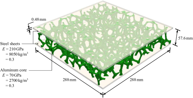
(a) Geometry of the sandwich panel

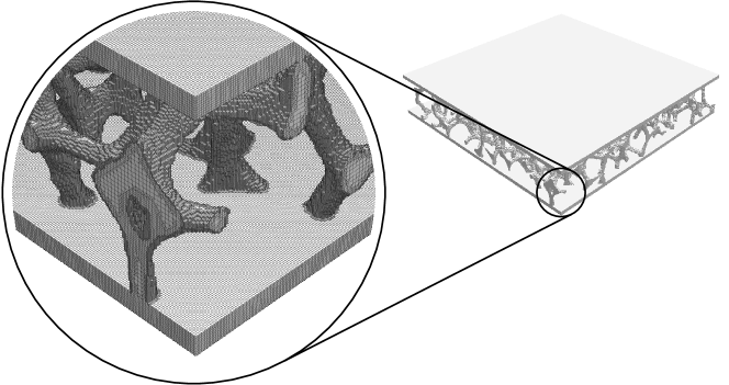
(b) Mesh of the sandwich panel

Figure 33: Geometry and mesh of the sandwich panel

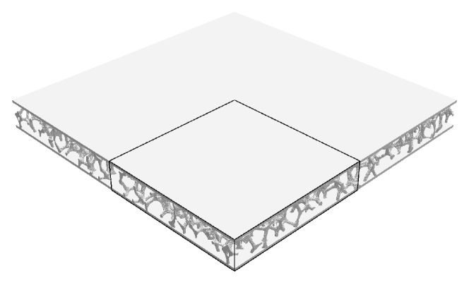
(a) $2\times 2$ panel

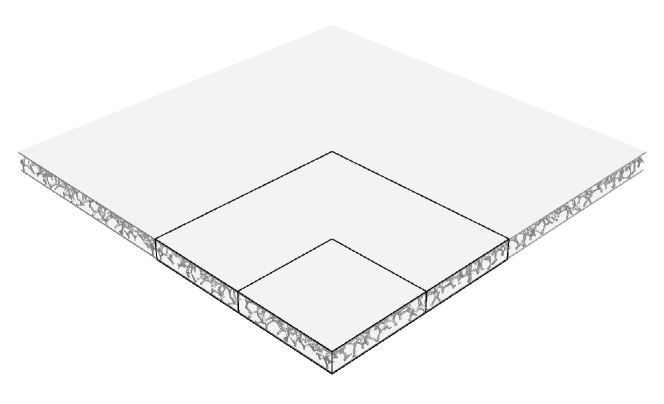
(b) $4\times 4$ panel

Figure 34: Mirroring operation of the sandwich panel

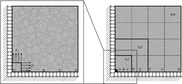
Figure 35: Boundary condition of the sandwich panel with an enlarged view of the loading area (left)

The mesh corresponding to the $4\times 4$ panel can be naturally divided into 16 parts by the mirror planes, and each part is further divided into 1024 parts, as shown in C. The top and bottom views of the magnitude of the displacement response at five time instances are presented in Fig. 36, illustrating the wave propagation process. It can be observed that the wave in the top panel disperses into the core and eventually to the bottom panel. The displacement and acceleration of four selected points shown in Fig. 35 (coordinates are $D\!\left(288,0,57.6\right)$, $F\!\left(576,0,57.6\right)$, $G\!\left(864,0,57.6\right)$ and $H\!\left(1152,0,57.6\right)$, unit: mm) are plotted in Fig. 37. The speedup of the multiple cores is illustrated in Fig. 38 and Table 5.

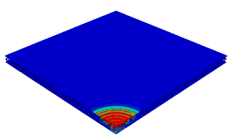
(a) Top view, $t=0.04\,\mathrm{ms}$

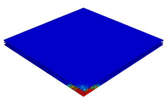
(b) Bottom view, $t=0.04\,\mathrm{ms}$

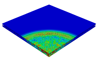
(c) Top view, $t=0.12\,\mathrm{ms}$

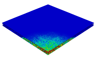
(d) Bottom view, $t=0.12\,\mathrm{ms}$

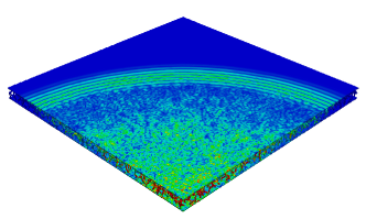
(e) Top view, $t=0.2\,\mathrm{ms}$

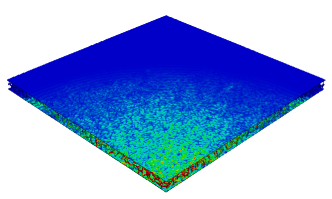
(f) Bottom view, $t=0.2\,\mathrm{ms}$

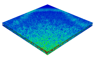
(g) Top view, $t=0.28\,\mathrm{ms}$

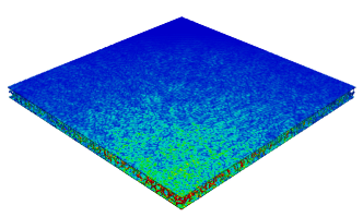
(h) Bottom view, $t=0.28\,\mathrm{ms}$

Figure 36: Contour of displacement magnitude at various time instances $t$

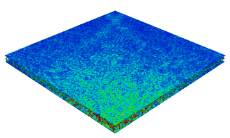
(i) Top view, $t=0.36\,\mathrm{ms}$

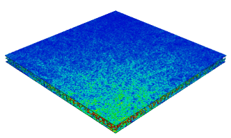
(j) Bottom view, $t=0.36\,\mathrm{ms}$

Figure 36: Contour of displacement magnitude at various time instances $t$

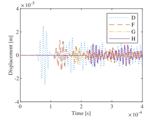
(a) Displacement of four points in the sandwich panel

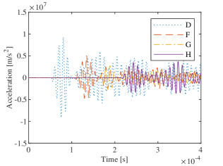
(b) Acceleration of four points in the sandwich panel

Figure 37: Response history of selected points of the sandwich panel

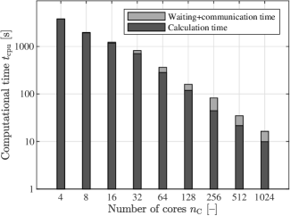
(a) Computational time of $1\times 1$ panel

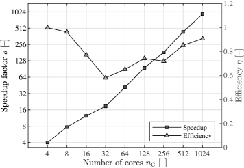
(b) Speedup and efficiency of $1\times 1$ panel

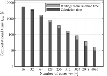
(c) Computational time of $2\times 2$ panel

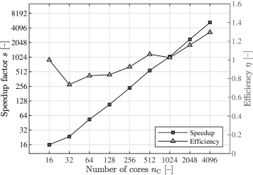
(d) Speedup and efficiency of $2\times 2$ panel

(e) Computational time of $4\times 4$ panel

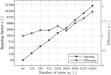
(f) Speedup and efficiency of $4\times 4$ panel

Figure 38: Time and speedup using multiple cores for the sandwich panel

Table 4: Computational time of the sandwich panel

$N_{\mathrm{cores}}$	$1\times 1$ panel			$2\times 2$ panel			$4\times 4$ panel
	$t_{\mathrm{C}}$ [s]	$t_{\mathrm{W}}$ [s]	$t_{\mathrm{T}}$ [s]	$t_{\mathrm{C}}$ [s]	$t_{\mathrm{W}}$ [s]	$t_{\mathrm{T}}$ [s]	$t_{\mathrm{C}}$ [s]	$t_{\mathrm{W}}$ [s]	$t_{\mathrm{T}}$ [s]
4	3790.78	12.54	3803.67	-	-	-	-	-	-
8	1937.86	36.19	1974.24	-	-	-	-	-	-
16	1175.07	55.04	1230.24	5317.17	232.99	5550.67	-	-	-
32	709.82	108.81	818.73	3253.78	514.92	3769.13	-	-	-
64	283.48	81.35	364.87	1320.66	347.40	1668.21	6316.70	1780.27	8097.55
128	119.05	41.04	160.11	620.23	204.36	824.66	2699.81	1010.44	3710.49
256	44.49	38.07	82.57	258.58	115.88	374.49	1184.53	516.15	1700.79
512	21.61	13.25	34.87	120.45	43.02	163.48	553.94	297.26	851.26
1024	9.92	6.46	16.37	47.45	37.05	84.63	264.50	115.35	379.87
2048	-	-	-	19.60	17.82	37.42	103.23	111.36	214.60
4096	-	-	-	9.81	6.92	16.73	42.76	45.70	88.46
8192	-	-	-	-	-	-	18.30	28.78	47.08
16384	-	-	-	-	-	-	9.81	7.60	17.41
$t_{\mathrm{C}}$: Calculation time
$t_{\mathrm{W}}$: Waiting and communication time
$t_{\mathrm{T}}$: Total time

Table 5: Speedup and efficiency of the sandwich panel

$N_{\mathrm{cores}}$	$1\times 1$ panel		$2\times 2$ panel		$4\times 4$ panel
	$s$	$\eta$	$s$	$\eta$	$s$	$\eta$
4	4.00	1.00	-	-	-	-
8	7.71	0.96	-	-	-	-
16	12.37	0.77	16.00	1.00	-	-
32	18.58	0.58	23.56	0.74	-	-
64	41.70	0.65	53.24	0.83	64.00	1.00
128	95.03	0.74	107.69	0.84	139.67	1.09
256	184.27	0.72	237.15	0.93	304.71	1.19
512	436.36	0.85	543.25	1.06	608.80	1.19
1024	929.21	0.91	1049.42	1.02	1364.27	1.33
2048	-	-	2373.29	1.16	2414.93	1.18
4096	-	-	5309.59	1.30	5858.25	1.43
8192	-	-	-	-	13028.57	1.59
16384	-	-	-	-	29775.04	1.82
$s$: Speedup factor
$\eta$: Efficiency

It can be observed that the CPU time increases with the number of DOFs slightly more than linearly. For a fixed number of cores, better efficiency can be achieved when the scale of the problem increases. In the analysis of the $1\times 1$ panel, a speedup factor of 929 is obtained when 1024 cores are used. In the $2\times 2$ panel, the maximum speedup is 5308 when using 4096 cores. In the $4\times 4$ panel, a speedup factor of 29760 is obtained with 16384 cores. It is noted that these values are calculated based on the assumption that $100\%$ efficiency is achieved when using the lowest number of cores, e.g., 4, 16 and 64, respectively. It is observed that for a fixed problem scale, the efficiency can increase with the number of cores in some cases, and some of the values are even higher than 1. This super-linear speedup is caused by the cache effect, i.e., as the mesh is partitioned and distributed to more cores, more data can be fit into the cache memory of the compute nodes, which has significantly higher data processing speed than RAM.

6 Summary

In this article, a parallel explicit solver for structural dynamics based on the CDM is developed, exploiting the inherent advantages of octree meshes. In our implementation, the octree meshes are efficiently handled by the SBFEM, which is our method of choice. However, it is important to note that exactly the same approach can also be applied to FEA when special transition elements with well-conditioned lumped mass matrices are deployed. These could be based on transfinite mappings [75, 27], virtual elements [10], etc. A special mass lumping technique is deployed by extending the work reported in Ref. [47] to 3D, yielding a well-conditioned diagonal mass matrix. The advantages of an explicit time integrator are leveraged, which enables the nodal displacements to be computed without the need for solving a system of linear equations. The pre-computation approach for the stiffness and mass matrices, relying on a limited number of unique octree cells in balanced meshes, further improves the efficiency of the algorithm.

The performance of the massively parallel explicit solver using the octree mesh generation and the SBFEM is demonstrated by means of five numerical examples, including academic benchmark problems with simple geometry as well as image and STL based models. Large-scale problems with up to one billion DOFs are simulated while up to 16,384 computing cores are utilized. The octree algorithm provides a fully automatic approach for mesh generation of complex geometric model. A Ricker wavelet, a triangular pulse load and a sine-burst signal are considered in these examples to excite the structures and to illustrate realistic and high-resolution engineering applications. Compared to a conventional (serial) implementation, a significant speedup is observed using the parallelization approach on multi-processor machines, and the in-house code can achieve an improved efficiency compared to the commercial software ABAQUS. In the current approach, the imbalance of workload of individual processors hinders a better scalability, as some processors have to wait for the slower processors to finish the job so that the results can be synchronized. In the future applications, a dynamic partitioning approach and a load distribution of the job based on the availability of individual processors may further improve the performance of the proposed algorithm. In addition, non-linear analyses, such as damage and contact problems can be studied making use of the novel methodology.

Appendix A Unique octree patterns in 3D

The unique octree patterns with hanging nodes on zero to six edges are listed. The remaining cases (seven to twelve hanging nodes) can be obtained from these cases, e.g., the first case of an octree cell with seven hanging nodes can be obtained from the first case with five hanging nodes by swapping the edges with and without hanging nodes, as shown in Fig. 46. The hanging nodes at the center of faces are not shown, which will be added following the discretization patterns.

Figure 39: Octree cell without hanging node

Figure 40: Octree cell with hanging node on one edge

Figure 41: Octree cells with hanging nodes on two edges

Figure 42: Octree cells with hanging nodes on three edges

Figure 43: Octree cells with hanging nodes on four edges

Figure 44: Octree cells with hanging nodes on five edges

Figure 45: Octree cells with hanging nodes on six edges

Figure 46: Octree cells with hanging nodes on seven edges (right) can be obtained from those with five edges (left)

Appendix B Mesh partition of the mountainous region

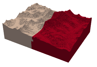
(a) two parts

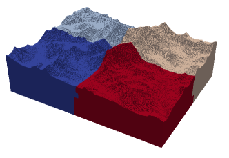
(b) four parts

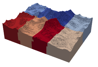
(c) eight parts

(d) 16 parts

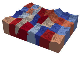
(e) 32 parts

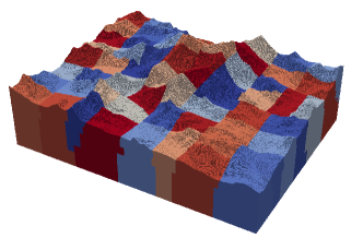
(f) 64 parts

Figure 47: Mesh partition of the mountainous region

Appendix C Mesh partition of the sandwich panel

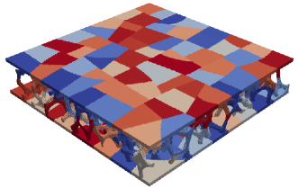
(a) 128 parts

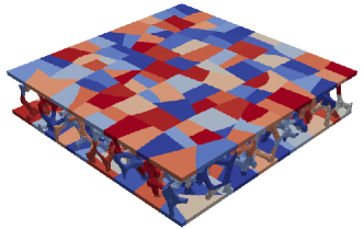
(b) 256 parts

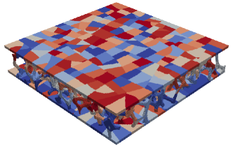
(c) 512 parts

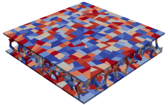
(d) 1024 parts

Figure 48: Mesh partition of the $1\times 1$ sandwich panel

References

- Dupros et al. [2010] F. Dupros, F. De Martin, E. Foerster, D. Komatitsch, J. Roman, High-performance finite-element simulations of seismic wave propagation in three-dimensional nonlinear inelastic geological media, Parallel Computing 36 (2010) 308–325.
- Brun et al. [2012] M. Brun, A. Batti, A. Limam, A. Gravouil, Explicit/implicit multi-time step co-computations for blast analyses on a reinforced concrete frame structure, Finite Elements in Analysis and Design 52 (2012) 41–59.
- Bettinotti et al. [2017] O. Bettinotti, O. Allix, U. Perego, V. Oancea, B. Malherbe, Simulation of delamination under impact using a global-local method in explicit dynamics, Finite Elements in Analysis and Design 125 (2017) 1–13.
- Zhang and Chauhan [2019] J. Zhang, S. Chauhan, Fast explicit dynamics finite element algorithm for transient heat transfer, International Journal of Thermal Sciences 139 (2019) 160–175.
- Meister et al. [2020] F. Meister, T. Passerini, V. Mihalef, A. Tuysuzoglu, A. Maier, T. Mansi, Deep learning acceleration of total Lagrangian explicit dynamics for soft tissue mechanics, Computer Methods in Applied Mechanics and Engineering 358 (2020) 112628.
- Cook et al. [1989] R. Cook, D. Malkus, M. Plesha, Concepts and applications of finite element analysis, Wiley, 1989.
- Patzák et al. [2001] B. Patzák, D. Rypl, Z. Bittnar, Parallel explicit finite element dynamics with nonlocal constitutive models, Computers & Structures 79 (2001) 2287–2297.
- Talebi et al. [2012] H. Talebi, C. Samaniego, E. Samaniego, T. Rabczuk, On the numerical stability and mass-lumping schemes for explicit enriched meshfree methods, International Journal for Numerical Methods in Engineering 89 (2012) 1009–1027.
- Li et al. [2014] B. Li, M. Stalzer, M. Ortiz, A massively parallel implementation of the optimal transportation meshfree method for explicit solid dynamics, International Journal for Numerical Methods in Engineering 100 (2014) 40–61.
- Park et al. [2019] K. Park, H. Chi, G. H. Paulino, On nonconvex meshes for elastodynamics using virtual element methods with explicit time integration, Computer Methods in Applied Mechanics and Engineering 356 (2019) 669–684.
- Anitescu et al. [2019] C. Anitescu, C. Nguyen, T. Rabczuk, X. Zhuang, Isogeometric analysis for explicit elastodynamics using a dual-basis diagonal mass formulation, Computer Methods in Applied Mechanics and Engineering 346 (2019) 574–591.
- Rek and Němec [2016] V. Rek, I. Němec, Parallel computation on multicore processors using explicit form of the finite element method and C++ standard libraries, Journal of Mechanical Engineering 66 (2016) 67–78.
- Altman [2014] Y. M. Altman, Accelerating MATLAB Performance: 1001 tips to speed up MATLAB programs, CRC Press, 2014.
- Ma et al. [2020] Z. Ma, Y. Lou, J. Li, X. Jin, An explicit asynchronous step parallel computing method for finite element analysis on multi-core clusters, Engineering with Computers 36 (2020) 443–453.
- Tang et al. [2020] J. Tang, Y. Zheng, C. Yang, W. Wang, Y. Luo, Parallelized implementation of the finite particle method for explicit dynamics in GPU, Computer Modeling in Engineering & Sciences 122 (2020) 5–31.
- Song and Wolf [1997] C. Song, J. P. Wolf, The scaled boundary finite-element method–alias consistent infinitesimal finite-element cell method–for elastodynamics, Computer Methods in Applied Mechanics and Engineering 147 (1997) 329–355.
- Deeks and Wolf [2002] A. J. Deeks, J. P. Wolf, An h-hierarchical adaptive procedure for the scaled boundary finite-element method, International Journal for Numerical Methods in Engineering 54 (2002) 585–605.
- Song [2004] C. Song, A super-element for crack analysis in the time domain, International Journal for Numerical Methods in Engineering 61 (2004) 1332–1357.
- Bazyar and Song [2008] M. H. Bazyar, C. Song, A continued-fraction-based high-order transmitting boundary for wave propagation in unbounded domains of arbitrary geometry, International Journal for Numerical Methods in Engineering 74 (2008) 209–237.
- Ooi et al. [2020] E. T. Ooi, M. D. Iqbal, C. Birk, S. Natarajan, E. H. Ooi, C. Song, A polygon scaled boundary finite element formulation for transient coupled thermoelastic fracture problems, Engineering Fracture Mechanics (2020) 107300.
- Chiong et al. [2014] I. Chiong, E. T. Ooi, C. Song, F. Tin-Loi, Scaled boundary polygons with application to fracture analysis of functionally graded materials, International Journal for Numerical Methods in Engineering 98 (2014) 562–589.
- Gravenkamp and Natarajan [2018] H. Gravenkamp, S. Natarajan, Scaled boundary polygons for linear elastodynamics, Computer Methods in Applied Mechanics and Engineering 333 (2018) 238–256.
- Talebi et al. [2016] H. Talebi, A. A. Saputra, C. Song, Stress analysis of 3D complex geometries using the scaled boundary polyhedral finite elements, Computational Mechanics 58 (2016) 697–715.
- Saputra et al. [2017] A. Saputra, H. Talebi, D. Tran, C. Birk, C. Song, Automatic image-based stress analysis by the scaled boundary finite element method, International Journal for Numerical Methods in Engineering 109 (2017) 697–738.
- Saputra et al. [2020] A. A. Saputra, S. Duczek, H. Gravenkamp, C. Song, Image-based 3D homogenisation using the scaled boundary finite element method, Computers & Structures 237 (2020) 106263.
- Gravenkamp et al. [2020] H. Gravenkamp, A. A. Saputra, S. Eisenträger, Three-dimensional image-based modeling by combining SBFEM and transfinite element shape functions, Computational Mechanics (2020) 1–20.
- Duczek et al. [2020] S. Duczek, A. Saputra, H. Gravenkamp, High order transition elements: The xNy-element concept-Part I: Statics, Computer Methods in Applied Mechanics and Engineering 362 (2020) 112833.
- Saputra et al. [2017] A. A. Saputra, V. Sladek, J. Sladek, C. Song, Micromechanics determination of effective material coefficients of cement-based piezoelectric ceramic composites, Journal of Intelligent Material Systems and Structures 29 (2017) 845–862.
- Gravenkamp and Duczek [2017] H. Gravenkamp, S. Duczek, Automatic image-based analyses using a coupled quadtree-SBFEM/SCM approach, Computational Mechanics 60 (2017) 559–584.
- Liu et al. [2019a] L. Liu, J. Zhang, C. Song, C. Birk, W. Gao, An automatic approach for the acoustic analysis of three-dimensional bounded and unbounded domains by scaled boundary finite element method, International Journal of Mechanical Sciences 151 (2019a) 563–581.
- Liu et al. [2019b] L. Liu, J. Zhang, C. Song, C. Birk, A. A. Saputra, W. Gao, Automatic three-dimensional acoustic-structure interaction analysis using the scaled boundary finite element method, Journal of Computational Physics 395 (2019b) 432–460.
- Xing et al. [2018] W. Xing, C. Song, F. Tin-Loi, A scaled boundary finite element based node-to-node scheme for 2D frictional contact problems, Computer Methods in Applied Mechanics and Engineering 333 (2018) 114–146.
- Xing et al. [2019] W. Xing, J. Zhang, C. Song, F. Tin-Loi, A node-to-node scheme for three-dimensional contact problems using the scaled boundary finite element method, Computer Methods in Applied Mechanics and Engineering 347 (2019) 928–956.
- Zhang and Song [2019] J. Zhang, C. Song, A polytree based coupling method for non-matching meshes in 3D, Computer Methods in Applied Mechanics and Engineering 349 (2019) 743–773.
- Gravenkamp et al. [2012a] H. Gravenkamp, J. Prager, A. A. Saputra, C. Song, The simulation of Lamb waves in a cracked plate using the scaled boundary finite element method, The Journal of the Acoustical Society of America 132 (2012a) 1358–1367.
- Gravenkamp et al. [2012b] H. Gravenkamp, C. Song, J. Prager, A numerical approach for the computation of dispersion relations for plate structures using the scaled boundary finite element method, Journal of Sound and Vibration 331 (2012b) 2543–2557.
- Gravenkamp et al. [2017] H. Gravenkamp, A. A. Saputra, C. Song, C. Birk, Efficient wave propagation simulation on quadtree meshes using SBFEM with reduced modal basis, International Journal for Numerical Methods in Engineering 110 (2017) 1119–1141.
- Zou et al. [2019] D. Zou, X. Teng, K. Chen, J. Liu, A polyhedral scaled boundary finite element method for three-dimensional dynamic analysis of saturated porous media, Engineering Analysis with Boundary Elements 101 (2019) 343–359.
- Zhang et al. [2020] J. Zhang, J. Eisenträger, S. Duczek, C. Song, Discrete modeling of fiber reinforced composites using the scaled boundary finite element method, Composite Structures 235 (2020) 111744.
- Liu et al. [2020] L. Liu, J. Zhang, C. Song, K. He, A. A. Saputra, W. Gao, Automatic scaled boundary finite element method for three-dimensional elastoplastic analysis, International Journal of Mechanical Sciences 171 (2020) 105374.
- Natarajan et al. [2020] S. Natarajan, P. Dharmadhikari, R. K. Annabattula, J. Zhang, E. T. Ooi, C. Song, Extension of the scaled boundary finite element method to treat implicitly defined interfaces without enrichment, Computers & Structures 229 (2020) 106159.
- Eisenträger et al. [2020] J. Eisenträger, J. Zhang, C. Song, S. Eisenträger, An SBFEM approach for rate-dependent inelasticity with application to image-based analysis, International Journal of Mechanical Sciences 182 (2020) 105778.
- Qu et al. [2020] Y. Qu, D. Zou, X. Kong, X. Yu, K. Chen, Seismic cracking evolution for anti-seepage face slabs in concrete faced rockfill dams based on cohesive zone model in explicit SBFEM-FEM frame, Soil Dynamics and Earthquake Engineering 133 (2020) 106106.
- Liu et al. [2017] Y. Liu, A. A. Saputra, J. Wang, F. Tin-Loi, C. Song, Automatic polyhedral mesh generation and scaled boundary finite element analysis of STL models, Computer Methods in Applied Mechanics and Engineering 313 (2017) 106–132.
- Song [2018] C. Song, The Scaled Boundary Finite Element Method: Introduction to Theory and Implementation, John Wiley & Sons, 2018.
- Zhang et al. [2020] J. Zhang, S. Natarajan, E. T. Ooi, C. Song, Adaptive analysis using scaled boundary finite element method in 3D, Computer Methods in Applied Mechanics and Engineering 372 (2020) 113374.
- Gravenkamp et al. [2020] H. Gravenkamp, C. Song, J. Zhang, On mass lumping and explicit dynamics in the scaled boundary finite element method, Computer Methods in Applied Mechanics and Engineering 370 (2020) 113274.
- Chan et al. [1994] T. F. Chan, J. R. Gilbert, S.-H. Teng, Geometric spectral partitioning, 1994.
- Song [2004] C. Song, A matrix function solution for the scaled boundary finite-element equation in statics, Computer Methods in Applied Mechanics and Engineering 193 (2004) 2325–2356.
- de Béjar and Danielson [2016] L. A. de Béjar, K. T. Danielson, Critical time-step estimation for explicit integration of dynamic higher-order finite-element formulations, Journal of Engineering Mechanics 142 (2016) 04016043.
- Duczek and Gravenkamp [2019a] S. Duczek, H. Gravenkamp, Mass lumping techniques in the spectral element method: On the equivalence of the row-sum, nodal quadrature, and diagonal scaling methods, Computer Methods in Applied Mechanics and Engineering 353 (2019a) 516–569.
- Duczek and Gravenkamp [2019b] S. Duczek, H. Gravenkamp, Critical assessment of different mass lumping schemes for higher order serendipity finite elements, Computer Methods in Applied Mechanics and Engineering 350 (2019b) 836–897.
- Krysl and Bittnar [2001] P. Krysl, Z. Bittnar, Parallel explicit finite element solid dynamics with domain decomposition and message passing: dual partitioning scalability, Computers & Structures 79 (2001) 345–360.
- Knuth [1974] D. E. Knuth, Postscript about NP-hard problems, SIGACT News 6 (1974) 15–16.
- Cvetkovic et al. [1980] D. M. Cvetkovic, M. Doob, H. Sachs, Spectra of Graphs, volume 10, Academic Press, New York, 1980.
- Gilbert et al. [1998] J. R. Gilbert, G. L. Miller, S.-H. Teng, Geometric mesh partitioning: Implementation and experiments, SIAM Journal on Scientific Computing 19 (1998) 2091–2110.
- Karypis and Kumar [1998] G. Karypis, V. Kumar, A fast and high quality multilevel scheme for partitioning irregular graphs, SIAM Journal on scientific Computing 20 (1998) 359–392.
- Ogawa [2003] T. Ogawa, Parallelization of an adaptive Cartesian mesh flow solver based on the 2N-tree data structure, in: K. Matsuno, A. Ecer, N. Satofuka, J. Periaux, P. Fox (Eds.), Parallel Computational Fluid Dynamics 2002, North-Holland, Amsterdam, 2003, pp. 441–448.
- LaSalle and Karypis [2016] D. LaSalle, G. Karypis, A parallel hill-climbing refinement algorithm for graph partitioning, in: 2016 45th International Conference on Parallel Processing (ICPP), IEEE, 2016, pp. 236–241.
- Li [2018] Y. Li, meshpart, https://github.com/YingzhouLi/meshpart, 2018.
- Willberg et al. [2012] C. Willberg, S. Duczek, J. Vivar Perez, D. Schmicker, U. Gabbert, Comparison of different higher order finite element schemes for the simulation of Lamb waves, Computer Methods in Applied Mechanics and Engineering 241 (2012) 246–261.
- Gravenkamp [2014] H. Gravenkamp, Numerical Methods for the Simulation of Ultrasonic Guided Waves, volume 116 of Dissertationsreihe, BAM-Berlin, 2014.
- Dalcín et al. [2005] L. Dalcín, R. Paz, M. Storti, MPI for Python, Journal of Parallel and Distributed Computing 65 (2005) 1108–1115.
- Dalcín et al. [2008] L. Dalcín, R. Paz, M. Storti, J. DElía, MPI for Python: Performance improvements and MPI-2 extensions, Journal of Parallel and Distributed Computing 68 (2008) 655–662.
- Dalcin et al. [2011] L. D. Dalcin, R. R. Paz, P. A. Kler, A. Cosimo, Parallel distributed computing using Python, Advances in Water Resources 34 (2011) 1124–1139.
- Chang et al. [2018] J. Chang, K. Nakshatrala, M. G. Knepley, L. Johnsson, A performance spectrum for parallel computational frameworks that solve PDEs, Concurrency and Computation: Practice and Experience 30 (2018) e4401.
- Chamberlin [2020] T. Chamberlin, Terrain2stl, https://www.jthatch.com/Terrain2STL/, 2020.
- Joulaian [2017] M. Joulaian, The Hierarchical Finite Cell Method for Problems in Structural Mechanics, VDI Fortschritt-Berichte Reihe 18 Nr. 348, 2017.
- Mossaiby et al. [2019] F. Mossaiby, M. Joulaian, A. Düster, The spectral cell method for wave propagation in heterogeneous materials simulated on multiple GPUs and CPUs, Computational Mechanics 63 (2019) 805–819.
- Nieuwenhius et al. [2005] J. H. Nieuwenhius, J. Neumann, D. W. Greve, I. J. Oppenheim, Generation and detection of guided waves using PZT wafer transducers, IEEE Transactions on Ultrasonics, Ferroelectrics, and Frequency Control 52 (2005) 2103–2111.
- Greve et al. [2005] D. W. Greve, J. J. Neumann, J. H. Nieuwenhius, I. J. Oppenheim, N. L. Tyson, Use of Lamb waves to monitor plates: Experiments and simulations, in: Proceedinggs of SPIE 5765, 2005.
- Giurgiutiu [2008] V. Giurgiutiu, Structural Health Monitoring with Piezoelectric Active Wafer Sensors: Fundamentals and Applications, Elsevier, 2008.
- Viktorov [1967] I. A. Viktorov, Rayleigh and Lamb Waves, Ultrasonic Technology, Plenum Press., 1967.
- Rose [1999] J. L. Rose, Ultrasonic Waves in Solid Media, Cambridge University Press, 1999.
- Provatidis [2019] C. G. Provatidis, Precursors of Isogeometric Analysis, Springer International Publishing, 2019.