Collective organisation and screening in two-dimensional turbulence

Abstract

Following recent evidence that the vortices in decaying two-dimensional turbulence can be classified into small–mobile, and large–quasi-stationary, this paper examines the evidence that the latter might be considered a ‘crystal’ whose formation embodies the inverse cascade of energy towards larger scales. Several diagnostics of order are applied to the ostensibly disordered large vortices. It is shown that their geometric arrangement is substantially more regular than random, that they move more slowly than could be expected from simple mean-field arguments, and that their energy is significantly lower than in a random reorganisation of the same vortices. This is traced to screening of long-range interactions by the preferential association of vortices of opposite sign, and it is argued that this is due to the mutual capture of corrotating vortices, in a mechanism closer to tidal disruption than to electrostatic screening. Finally, the possible relation of these ‘stochastic crystals’ to fixed points of the dynamical system representation of the turbulence flow is briefly examined.

I Introduction

This paper is part of a sequence that began as an investigation on whether an automatic computer search of ‘relevant’ features in decaying two-dimensional turbulence could be used to suggest new ideas about the organisation of the flow [1]. That paper was continued in [2, 3], mostly from the point of view of how such a search should be organised, and of its possible relation to automatic learning, and eventually led in [4] into an analysis of the flow itself. It is with the conclusions of this last paper that the present one deals.

Two-dimensional turbulence is a well-studied phenomenon, often used as an approximation to geophysical and stratified flows in which isotropy is broken by some constraint along the third dimension. Although truly two-dimensional turbulence is experimentally challenging, it was one of the first turbulent flows to become accessible to direct numerical simulation, and computational experiments were soon undertaken to test theoretical predictions [5, 6, 7, 8, 9]. Much of its theoretical interest can be traced to the early observation in [10] that a system of point vortices in a plane could lead, under some conditions, to states of negative temperature and to the formation of large-scale structures. We will see later that the point-vortex model is a poor approximation to turbulence, because the former is Hamiltonian, and conserves enstrophy (the square of vorticity) and kinetic energy, while the later is dissipative, but the statistical mechanics of point vortices has continued to be examined in the hope that it may be locally relevant to the dissipative case [6, 11, 12]. Dissipative mean-field theories based on cascades of the inviscidly conserved quantities were developed almost simultaneously to the Hamiltonian model [13, 5], eventually leading to the prediction of a direct cascade of enstrophy towards smaller scales, and an inverse cascade of energy towards larger ones [13, 14]. The latter could intuitively be related to the negative-temperature states of [10].

However, simulations showed that the flow spontaneously segregates into coherent vortices and a less-coherent background, and that the vortices interfere with the conclusions of the mean-field representation. By the end of the 1990’s there was widespread consensus that two-dimensional turbulence is a vortex gas, following approximately Hamiltonian dynamics punctuated by occasional mergings of vortices of like sign. The forward enstrophy cascade proceeds by successive vortex merging and filamentation [15, 16, 17, 18], and is not described well by mean-field theories. The mechanism of the backwards energy cascade is less clear, although it is not believed to be associated with the formation of larger vortices by amalgamation [19, 20, 21, 22], but the phenomenon itself has been observed numerically, especially in forced systems kept in statistical equilibrium by a large-scale dissipation mechanism [23, 24]. In a finite domain, and in the absence of a dissipation mechanism, the energy accumulates at the largest available flow scale, in a phenomenon akin to Bose-Einstein condensation [25, 26] and to the predictions in [10]. Fuller reviews of previous work on two-dimensional turbulence can be found in [27, 28].

The results in [4] extended the previous models in some interesting directions, especially regarding the decay of unforced turbulence in the early period in which the spectral scale of the energy has not grown enough to be affected by the simulation domain. It was found that the largest structures of the kinetic energy take the form of elongated high-speed jets, flanked by a subset of large vortices that move relatively slowly with respect to the global root-mean square (r.m.s.) velocity. The cascade of energy towards large scales corresponds to the growth of these jets. It was speculated in [4] that the slowly moving vortex dipoles that flank the jets form a large-scale collective structure that can approximately be described as a ‘crystal’, and it was further speculated that the formation of the dipoles responds to a tendency of the flow to organise into low-energy configurations. This will be shown below to be the case, even if it may be considered counter-intuitive in a system, like two-dimensional turbulence, which dissipates enstrophy rather than energy, and in which the latter could be expected to ‘lag behind’ the decay of the former.

The questions addressed in the present paper concern this possible collective structure. After describing in §II the generation of the data and their general properties, we examine in §III whether the flow really is in a low-energy state, and whether this is connected with the presence of dipoles. Section IV looks at the question of vortex mobility, and §V and §VII discuss whether the organisation of the large vortices is regular enough to be considered a crystal, even approximately.

Two related questions are addressed in the context of the previous results. The first one is whether there is any screening between vortices of different sign, as originally suggested by [29], and the second one is whether the vortex ‘crystal’ described above could be related to the fixed-point solutions that have been invoked as organising states for high-dimensional or turbulent dynamical systems [30]. Discussion of these and other questions, and conclusions, are offered in §VI and §VIII.

II Numerical experiments

The data used in this paper are mostly those in [4], to where the reader is referred for details. Simulations of decaying nominally isotropic two-dimensional turbulence are performed in a doubly periodic square box of side $L$, using a standard spectral Fourier code dealiased by the 2/3 rule. Time advance is third-order Runge-Kutta. The flow field is defined by its velocity $\boldsymbol{u}=(u,v)$ in the $\boldsymbol{x}=(x,y)$ plane, and by the one-component vorticity $\omega=\nabla\times\boldsymbol{u}$. It is initialised with random Fourier phases and a fixed isotropic enstrophy spectrum whose peak, approximately located at wavenumber $k_{init}=2\pi/L_{init}$, controls the initial width of the energy-containing spectral range. The equations are solved in vorticity–stream-function formulation, using regular second-order viscosity, $\nu\nabla^{2}\omega$, and the flow is evolved for a fixed time to allow vortical structures to establish themselves. This moment is defined as $t=0$, and denoted by a ‘0’ subindex in the corresponding quantities. Experiments are run as ensembles of at least 768 flows, with more samples added in some cases to improve statistics. Case T1024a, which was not in [4], has been included to provide a wider initial range of scales. As the simulation proceeds, the enstrophy $\langle\omega^{2}\rangle$, where the time-dependent average $\langle\cdot\rangle$ is taken over the full computational box and over the ensemble, decays by approximately 70–80%, while the kinetic energy, $\langle|\boldsymbol{u}|^{2}\rangle$, decreases by at most 15–20% (figure 1a). The numerical parameters for the different cases are summarised in table 2. The time step is controlled by a CFL condition $N|\boldsymbol{u}|_{max}\Delta t/3=0.5$, and T1024a was repeated with a twice shorter time step to confirm the numerics.

Table 1: Parameters of the simulations. The size of the doubly periodic computational box is $L\times L$. The r.m.s. vorticity $\omega_{0}^{\prime}$, and the velocity magnitude $q_{0}^{\prime}$, are measured after the initial discarded transient, decaying from an initial enstrophy spectrum whose peak is at wavelength $L_{init}$. The enstrophy and energy scales, $\lambda_{\omega 0}$ and $\lambda_{q0}$, are defined in the text. The number of collocation points used for dealiasing is $N\times N$. The subscript ‘F’ refers to the end of each simulation, and the decay time after the initial transient, $t_{F}$, is chosen so that $\lambda_{qF}/L\approx 0.6$. Each case is an ensemble of $N_{t}$ independent experiments. For details, see [4].

Case	$N$	$L_{init}/L$	$q^{\prime}_{0}L/\nu$	$N_{t}$	$\lambda_{\omega 0}/L$	$\lambda_{q0}/L$	$\omega^{\prime}_{0}t_{F}$	$\omega^{\prime}_{F}/\omega^{\prime}_{0}$	$q^{\prime}_{F}/q^{\prime}_{0}$	Symbol
T512	512	0.05	4400	768	0.129	0.256	23.0	0.50	0.91	$\scriptstyle\triangle$
T768	768	0.025	7800	768	0.108	0.217	39.4	0.49	0.92	$\scriptscriptstyle\bigtriangledown$
T1024	1024	0.033	11000	1392	0.095	0.197	51.3	0.40	0.92	$\scriptstyle\Box$
T1024a	1024	0.01	8900	2304	0.078	0.142	65.4	0.31	0.87	$\circ$

Natural time and velocity scales can be defined from the r.m.s. vorticity magnitude $\omega^{\prime}=\langle\omega^{2}\rangle^{1/2}$ and from $q^{\prime}=(u^{\prime 2}+v^{\prime 2})^{1/2}$. The two length scales mainly used in [4] are the energy spectral wavelength $\lambda_{q}=2\pi/k_{q}$, defined by the maximum of the premultiplied energy spectrum $kE_{qq}(k)$, where $k$ is the wavenumber magnitude, and the enstrophy wavelength, $\lambda_{\omega}$, similarly defined from the enstrophy spectrum, $kE_{\omega\omega}$. Both scales increase with time, but $\lambda_{q}$ increases faster than $\lambda_{\omega}$, reflecting the energy flow towards larger scales [13]. They are not proportional to each other, and describe different flow features. It was shown in [4] that $\lambda_{\omega}$ is proportional to the diameter of individual vortices, defined as connected objects in which the vorticity magnitude is larger than $\omega^{\prime}$, while $\lambda_{q}$ measures the average distance, $d$, between closest neighbouring vortices of similar size. Our simulations are discontinued when $\lambda_{q}/L\approx 0.6$, beyond which the flow is considered to enter a different decay regime in which the energy transfer towards larger scales is substantially modified by the finite box. As already mentioned in the introduction, vortices naturally separate into two classes. Those whose circulation, $\gamma_{i}$, is weaker than the mean, $|\gamma_{i}|<\langle|\gamma_{i}|\rangle$, tend to move fast, have a power-law distribution of area and circulation, and are only responsible for a small fraction of the total kinetic energy of the flow [4]. Vortices stronger than the mean move more slowly, have an exponential probability distribution (figure 1b), and are responsible for most of the kinetic energy. This was interpreted in [4] to mean that the large vortices form a ‘crystal’ in approximate equilibrium, which is the subject of the present paper. From now on, although the simulations are always run without truncation, our analysis refers to the fraction of the flow reconstructed from the large vortices, once the smaller ones have been deleted.

Deleting vorticity from a periodic flow usually requires some correction, because periodicity of the velocity field is only possible if the overall circulation vanishes,

$$\sum_{i}\gamma_{i}=0.$$ (1)

When this is not satisfied, it has to be compensated by a background uniform vorticity, $-\sum\gamma_{i}/L^{2}$. We will see below that the total kinetic energy of the flow is proportional to the integrated squared circulation [31], so that the expected relative error of the energy estimates in the following section is of the order of $\left(\sum\gamma_{i}\right)^{2}/\sum\gamma_{i}^{2}$. In our reconstructed flows, it is at most $O(10^{-4})$.

Figure 1: (a) Evolution of the enstrophy (open symbols), and energy (closed symbols) of the simulations in table 2. Symbols as in the table. Colours are: red, T512; blue, T768; magenta, T1024; green, T1024a. They are used whenever possible throughout the paper. (b) Probability density functions of the vortex circulation. Only vortices with $\gamma/\langle\gamma\rangle>1$ are included in the reconstructed flow fields. (c) Comparison of the Poisson wavelength (3), with the spectral wavelengths, $\lambda_{q}$ (open symbols), and $\lambda_{\omega}$ (closed symbols). The dashed line is $\lambda_{q}=\lambda_{P}$. (d) Open symbols are the mean distance between neighbouring large vortices, and closed symbols are the mean diameter of the large vortices, both versus $\lambda_{P}/L$. The dashed line is $\langle d\rangle=0.27\lambda_{P}$, and the solid one is $\langle s^{1/2}\rangle=0.21\lambda_{P}$.

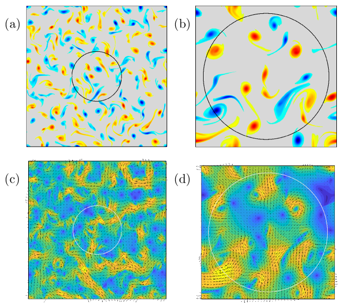
Figure 2: (a,b) Flow vorticity synthesised by retaining only vortices whose area is larger than the average, in one of the members of the T1024a ensemble. The circle in each case has radius $\lambda_{P}$. (a) $\omega_{0}^{\prime}t=1.3$, $\lambda_{P}/L=0.18$. (b) $\omega_{0}^{\prime}t=52.3$, $\lambda_{P}/L=0.45$. (c,d) Velocity field for the flows in (a,b), respectively. The background colour is the velocity magnitude, lighter for faster velocities.

It follows from the proportionality between $d$ and $\lambda_{q}$ that the average number of large vortices per flow field should decay as $(\lambda_{q}/L)^{-2}$. Empirically,

$$n_{v}\approx 4(L/\lambda_{q})^{2},$$ (2)

which decays from approximately 150 to 15 in our simulations. The last number approximately agrees with [8], who studied similar flows at longer decay times, where $\lambda_{q}$ saturates to approximately $L$, and reported that the motion of the 17 largest vortices was approximately independent of their background. The number of small vortices is approximately twice higher than of those larger than the mean. Because counting large vortices is a more stable operation than finding the maximum of a noisy spectrum, especially in the late stages of the evolution in which the definition of $\lambda_{q}$ depends on a few low-wavenumber harmonics, we will use in the following a ‘Poisson’ wavelength inspired by (2),

$$\lambda_{P}/L=2n_{v}^{-1/2}.$$ (3)

The relation between $\lambda_{P}$ and the two spectral wavelengths is shown in figure 1(c). Figure 1(d) shows its relation to the mean distance between large vortices, and to their diameter. It is not surprising that $\lambda_{P}$ is proportional to the distance between vortices, because this is how it is defined. In fact, assuming that the vortices are a Poisson-distributed set of points with density $n_{v}/L^{2}$, their average separation would be $\langle d\rangle=0.5L/n_{v}^{1/2}=0.25\lambda_{P}$ [4]. This linear dependence, and even its coefficient, are well satisfied in figure 1(d).

More interesting is that $\lambda_{P}$ is also linearly related to the vortex diameter, $\langle s^{1/2}\rangle$, where $s$ is the area of the thresholded vortices. This was not the case for the full vortex system analysed in [4], where the diameter was found to be proportional to $\lambda_{\omega}$, which is not proportional to $\lambda_{q}$. Figure 1(d) implies that, even if the decay of the full flow is not self-similar in this way, the decay of the system of large vortices is truly self-similar, with a vortex diameter proportional to the separation. Two snapshots of the temporal evolution of the large-vortex component of a turbulent flow are shown in figure 2. The circles in the figure have radius $\lambda_{P}$, and (3) implies the number of vortices within them should stay approximately equal to $4\pi$. The figure also displays the velocity field of these two flows, clearly showing the high-velocity streams mentioned in the introduction [4].

Although not discussed in detail in this paper, reference will occasionally be made to simulations of Hamiltonian systems of point vortices. Their characteristics and numerical details are described in Appendix A.

III The kinetic energy

The clearest indication that the arrangement of the large vortices is not random is figure 3, which compares the total kinetic energy of an ensemble of large-vortex reconstructions of turbulent flows with that of another ensemble in which the position of the same vortices is randomised. Figures 3(a,b) are joint probability density functions (p.d.f.) of the kinetic energy of the members of the ensemble,

$$K=L^{-2}\int_{L^{2}}|\boldsymbol{u}|^{2}{\,\rm{d}}^{2}\boldsymbol{x},$$ (4)

versus the energy required for randomisation, $K_{\Delta}=K-K_{s}$. Particularly at the earlier evolution time in figure 3(a) (one of whose members is represented in figure 2a), the scrambling of the vortex position almost always leads to higher energies, although the effect weakens as the flow evolves towards fewer vortices in figures 3(b) and 2(b). Some caution is required in interpreting this result, because the vortices occasionally overlap after being rearranged, modifying the total enstrophy and the energy. The overlap is of the order of 7-10% of the vortex area, and, while the effect on the enstrophy is statistically neutral (not shown), that on the kinetic energy is not. Its magnitude is tested in figure 3(a,b) by repeating the scrambling experiment after substituting each vortex by a compact ‘point’ core with the same circulation, located at its centre of gravity (see appendix A). The overlap then decreases by a factor of 2 to 10 (see appendix B), depending on the case, but the effect of the scrambling is still to increase the energy. Figure 3(c) summarises the energy increase for all the experiments and evolution times. The best collapse is obtained by plotting it against $\lambda_{P}/L$, or, equivalently, against the number of vortices in the periodic domain.

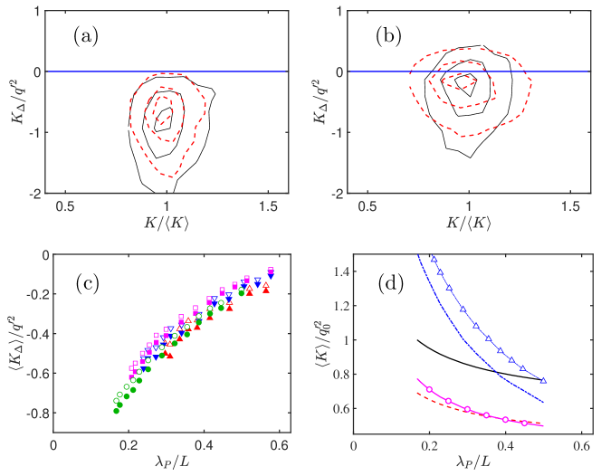
Figure 3: (a) Joint probability density function of the kinetic energy difference, $K_{\Delta}=K-K_{s}$, between the extended-vortices flows, $K$, and the same flow in which the vortex positions are randomised, $K_{s}$. T1024a at the time of figure 2(a). (b) As in (a), at the time of figure 2(b). (c) Ensemble average of the randomising energy, versus $\lambda_{P}$. Symbols as in table 2. In (a-c), open symbols and solid lines are the turbulence vortices, and closed symbols and dashed lines are the point-vortex approximation. Contours in (a,b) contain 10%, 50% and 90% of the probability. (d) Kinetic energy evolution.   , Total kinetic energy;            , energy from all vortices;    $\circ$    , energy from large vortices;                   , energy from scrambled large vortices;    $\scriptstyle\triangle$   , self-energy approximation to the scrambled large vortices. T1204a.

The kinetic energy of a sparse zero-circulation system of two-dimensional small vortices is [32, §7.3],

$$2\pi K\approx\left(\sum_{i}\gamma_{i}^{2}\right)\log(\delta/\ell)+\sum_{i}\sum_{j\neq i}\gamma_{i}\gamma_{j}\log(r_{ij}/\ell)+\ldots,$$ (5)

where $r_{ij}$ is the distance between vortices, $\ell$ is an arbitrary length scale, and $\delta$ is of the order of the radius of the vortex cores. The first term in the right-hand side of this equation is the self energy, and is independent of the vortex position. It derives from the $1/r$ velocity in the neighbourhood of the cores, and diverges as $\log(\delta)$. The second term in (5) is the interaction energy. It is independent of $\delta$, and only depends on the relative vortex position.

When (5) is modified to take into account the spatial periodicity of the computational box, the argument of the logarithms gains a Jacobian elliptic function [33], which does not change the short-range interactions but introduces $\ell=L$ as a natural length scale. With this choice, the self-energy of the cores increases with decreasing core size, and is 2–3 times larger for the point-vortex model than for the extended vortices of the original turbulence. This is the reason why the abscissae in figure 3 have to be scaled with the individual average for each system, but the figure shows that the interaction energy spent in randomisation is the same for both flows, which is why their ordinates can be scaled with the same energy ($q^{\prime 2}$ of the turbulent flow).

One of the most intriguing features of figure 3(c) is that the magnitude of the available interaction energy is initially of the same order as the total kinetic energy of the flow, but that it almost vanishes at the end of the simulations. This appears to contradict the result in figure 1(a) that the kinetic energy stays approximately constant during the decay, and the implication is that most of the interaction energy is never expressed in the flow. The energy redistribution mechanism responsible for keeping vortices in a reduced-energy state is conservative, unrelated to dissipation, and the position of the vortices in a turbulent flow is always far from random.

Consider figure 3(d), which shows the evolution of several components of the energy of the flow as it decays. The black solid line is the total kinetic energy, which decays by about 20%. The same is approximately true of the part of the kinetic energy contained in the large vortices, which closely tracks the total. The approximately 20–25% separating the two energies is presumably contained in the incoherent background. Including the vortices that we have classified as small (red dashed line) does not change the picture [4]. They actually subtract some energy from the flow during most of the evolution. The largest energy reservoir is in the set of randomised vortices (blue chain-dotted line), which is almost exclusively self energy. The triangles in figure 3(d) are an approximation to the kinetic energy that essentially treats the first term in (5) as a sum of independent variables (see appendix C). It represent the data well, especially taking into account that the turbulence vortices are far from circular, and that the definition of $\delta=\langle(s/\pi)^{1/2}\rangle$, is ambiguous.

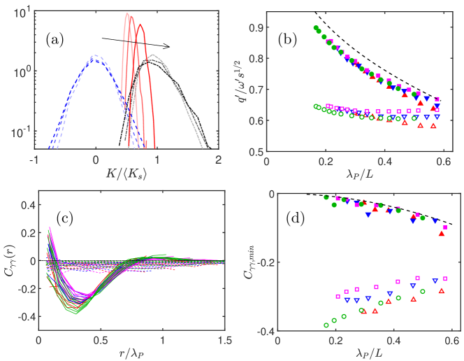
Figure 4: (a) One-dimensional p.d.f. of the kinetic energy of the reconstructed flows.   , Unscrambled vortices;                   , scrambled;            , difference between two scramblings of the same flow. T1024a. Time increases from light to dark, $\omega^{\prime}_{0}t=$ 1.3, 19.6, 52.3, and all energies are normalised with the mean scrambled energy at each time. (b) Normalised velocity intensity. Symbols as in table 2. Open symbols are unscrambled flows; solid ones are scrambled. The dashed line is the logarithmic correction (6). (c) Correlation of the vortex circulation as a function of their distance. All cases and times. Colours as in (b).   , unscrambled;            , scrambled. (d) Minimum of the correlations in (c). Symbols as in (b), but the dashed line is (8).

Figure 4(a) examines the energy distribution in more detail. The solid red lines are p.d.f.s of the kinetic energy for the ensemble of turbulent flows, plotted at three evolution times that increase in the direction of the arrow and of the darker shades of colour. In each case, the energy is normalised with the average energy of the ensemble of scrambled flows at the same time, and the rightward drift of the p.d.f. corresponds to the upward trend of the open symbols in figure 3(c). The black dashed lines in figure 4(a) are p.d.f.s of the energy of the scrambled flows, scaled with their own mean. They change little with time, and we have seen that they mostly include the self-energy of the vortices. It could be expected that, since the vortex positions are randomised, and since the velocity at each point of the flow is the sum of the contributions of the different vortices, the central-limit theorem would result in a Gaussian p.d.f., but [31] examined this limit, and concluded that the $1/r$ velocity distribution due to each core in a system of random compact vortices is marginal for the application of the central-limit theorem. Although the p.d.f. of the resulting velocity would tend to Gaussian for a very large number of vortices, the rate of convergence is too slow to be useful in any practical sense. As a consequence, the distributions in figure 4(a) are skewed, as in [31]. Finally, the blue chain-dotted curves in figure 4(a) are the interaction energy, which has been isolated by subtracting the energy of two different randomisations of the same flow, $K_{\Delta\Delta}=(K_{s1}-K_{s2})/\sqrt{2}$. These distributions are symmetric with zero mean, by construction, and, at least for the flows represented here, collapse well when scaled with the mean scrambled energy. Their standard deviation is of the order of 25–30% of this mean, proving that there is enough energy in the vortex interactions to explain the energy required for scrambling.

It is significant that the distribution of the energy within the ensemble of real flows is much narrower than in the scrambled ones, implying again that turbulence only explores a small subset of the possible vortex distributions. Figure 4(b) shows the scaling of the kinetic energy with the enstrophy. Dimensionally, $q^{\prime}\sim\omega^{\prime}\langle s\rangle^{1/2}$, where $\langle s\rangle$ is the average vortex area, but there is a logarithmic correction (appendix C), with the same origin as in figure 3(d),

$$q^{\prime 2}/\omega^{\prime 2}\langle s\rangle\sim\log(\ell_{0}/R),$$ (6)

where $\ell_{0}$ and $R$ are outer and inner limits, respectively, of the region over which the velocity induced by a vortex core decays as $1/r$. The inner scale is always of the order of the vortex radius $R\sim\langle s^{1/2}\rangle$, but $\ell_{0}$ depends on the vortex distribution. For a random distribution of vortices in a box of side $L$ we can assume $\ell_{0}\approx L/2$ and, since we saw in figure 1(d) that $\langle s^{1/2}\rangle\approx\lambda_{P}/4$, the right-hand side of (6) is approximately $\log(2L/\lambda_{P})$. The ratio $q^{\prime}/\omega^{\prime}\langle s^{1/2}\rangle$ is plotted in figure 4(b), where the difference between the scrambled and unscrambled flows is equivalent to the one in figure 3(c). It is plotted against $\lambda_{P}/L$, and the logarithmic correction (6) is included as a dashed line. It describes the trend of the randomised flows well. Interestingly, the normalised energy of the original turbulent flows satisfies the uncorrected constant scaling much more closely than the scrambled ones, consistent with $\ell_{0}/R\approx 1.5-2$. This suggests that the turbulence vortices suppress each other’s $1/r$ velocity field beyond distances of the order of $d/\lambda_{P}\approx 0.3-0.4$, which is also the typical distance between nearest neighbours.

That neighbouring vortices are not randomly distributed is confirmed by figure 4(c), which displays the correlation coefficient of vortex circulation as a function of distance,

$$C_{\gamma\gamma}(r)=\langle\gamma_{i}\gamma_{j}\rangle/\langle\gamma_{i}^{2}\rangle,$$ (7)

where $r=\langle r_{ij}\rangle$, and the average is taken over the ensemble and over all the $(i\neq j)$ combinations. Since, on average, there is the same number of vortices of each sign, one could expect this correlation to vanish. This is approximately true for the scrambled flows, plotted in the figure as dashed lines, but turbulent flows behave differently, and the correlation reaches a negative minimum at $r\approx 0.33\lambda_{P}$. This is close to the distance between neighbouring cores (figure 1d), and implies that near neighbours tend to be of opposite sign. We noted when discussing (3) that the distribution of distances among neighbouring vortices is consistent with a Poisson distribution, and the same is found in [4], but, when the vortices in that paper are grouped into closest pairs, the number of counter-rotating dipoles is found to be approximately 50% larger than that of co-rotating pairs. This effect disappears when the vortex position is randomised.

The minimum values of the correlations in figure 4(c) are collected in figure 4(d). Those from the turbulent flows increase slowly with increasing $\lambda_{P}/L$, but those from the scrambled ones do the opposite, and it is intriguing that they are always negative, even if they are independent of the distance $r$. This would seem to imply that some structure remains in the randomised flows, but the explanation is probably simpler, and, as we shall see below, significant. Consider a flow with $n_{v}$ identical vortices of balanced sign. Each vortex sees $n_{v}/2$ vortices of opposite sign, for which $\gamma_{i}\gamma_{j}<0$, but only $n_{v}/2-1$ vortices for which $\gamma_{i}\gamma_{j}>0$, discounting itself. Using (3), the resulting average is

$$C_{\gamma\gamma}\approx-1/n_{v}=-0.25(\lambda_{P}/L)^{2}.$$ (8)

This line has been added to figure 4(d), and represents the data well.

Screening of the far-field electrostatic potential by the redistribution of charges is well known in plasmas and electrolytes, where a charged particle induces a shell of charges of opposite sign that shelters its effect at long distance [34, §75]. This sheltering reduces the total potential energy, and it was speculated in [29] that a similar effect could be present in turbulence. There is little empirical or experimental evidence either way, although [35, 36] observed that the absence of long-range pressure correlations in simulations of three-dimensional isotropic turbulence could be due to screening, and generalised the argument to other three-dimensional flows. On the contrary, [31] found that a random vortex distribution describes well the second-order moments of decaying two-dimensional turbulence, and interpreted this as evidence for the absence of screening. The reason for this discrepancy with the present results is not clear, but the two simulations are difficult to compare, because [31] uses fourth-order hyperviscosity as a dissipation model. Hyperviscous vortices are typically smaller than viscous ones, and the area fraction covered by the vortices in that simulation is an order of magnitude smaller than in the present one. It is likely that $q^{\prime}$ in [31] is mostly self-energy

On the other hand, electrostatic screening is quite different from vortex rearrangement, as already noted in [29]. The electrostatic Debye–Hückel screening length arises from a balance between the potential energy of the charge distribution and the kinetic energy of thermal agitation [34]. The rationale for vorticity screening would also be to minimise total energy, and it was already speculated in [4] that the predominance of dipoles in simulations could be an energy effect. But, although it is clear from (5) that tight pairs of cores of opposite sign decrease the interaction energy with respect to those of the same sign, this is due to their effect on the kinetic energy in the far field. There is no potential energy among vortices, and calculations of the evolution of point vortex systems (see appendix A) reveal no screening effect. Their correlation coefficient (7) remains equal to zero up to an inner limit determined by the temporal resolution of the numerical scheme, and the distribution of distances among close vortices is consistent with Poisson statistics, both for pairs of the same sign and for dipoles.

In fact, the evolution of inviscid point vortices and the decay of two dimensional turbulence are fairly different problems, because, as mentioned in the introduction, the former is a Hamiltonian system that conserves energy, momentum and, by default, enstrophy, while the latter is dissipative. But there is persuasive evidence that they are not completely unrelated, and [8] showed that substituting points for the largest vortices in decaying turbulence reproduces well their motion for short times, while [17] showed that adding a simple merging rule for like-signed vortices, designed to conserve energy while dissipating enstrophy, extends the validity of the model to longer decays. On the other hand, if screening were just a local energy effect, it should be visible in the Hamiltonian simulations, which we have seen not to be the case. A fair amount of work has gone into the equilibrium solutions of sets of point vortices, from vortex crystals that are steady in some frame of reference [37] (see also §VI below), to maximum-entropy distributions which are only statistically stationary [6, 11]. These last two papers centre on the statistical mechanics of sets of point vortices, in terms of an interaction energy measured with respect to the random distribution. They find that, when the interaction energy is positive, the two vortex signs separate into large coherent regions of opposite circulation, as in the negative ‘temperature’ states in [10]. For negative energies, equivalent to positive temperatures, the two signs stay mixed. It follows from figures 3 and 4 that the latter is the regime of our decaying flows, except perhaps for distances of the order of the separation between immediate neighbours.

The closest equivalent to screening in the context of vortex flows is shear sheltering [38, 39, 40], in which a vortex approaching a strong vorticity interface deforms it in such a way as to cancel the long-range effect of the vortex. This has been invoked, for example, to explain the persistence of strong vortices in two-dimensional turbulence [39], and of regions of very different turbulence intensities in three-dimensional turbulence [40], but the effect is restricted to the interaction of vorticity structures of very different magnitude. Thus, while sheltering might be involved in the separation of vortex cores into large and small, it is unlikely to be the reason why the strong vortices rearrange themselves into low-energy configurations.

More promising is an extension of the argument leading to (8), and it may be relevant that, if this equation is extrapolated to $\lambda_{P}\approx L\,(n_{v}\approx 5)$, it approaches $C_{\gamma\gamma,min}\approx-0.25$, which is of the same order as the observed minima for the turbulence data. This, together with the observation that the negative correlations are restricted to distances of the order of the nearest vortex neighbours, suggests that the vortex circulation tends to be in balance over neighbourhoods of $O(\lambda_{P})$, in such a way that each vortex sees an excess of neighbours of the opposite sign. There are several ways in which this might be implemented. The simplest one is probably vortex amalgamation. When two point vortices are drawn together by a multi-vortex interaction, they tend to stay together for some time, among other reasons because separating them requires exchanging an energy that may not be locally available. This is true for point vortices of any sign, but the long term evolution of pairs of extended patches depends on their relative sign. Corrotating pairs tend to merge [41], so that one of the partners disappears from the local count, while counter-rotating dipoles are stable [42, 7]. This would explain the prevalence of dipoles over co-rotating pairs, and the local correlation minimum in turbulence simulations, as well as the absence of both effects in point-vortex systems.

Vortex amalgamation depends on the ratio of the vorticity to the strain that the partners induce on each other [43], which, for approximately similar vortices, only becomes relevant at distances of the order of the vortex radius [44]. This would be consistent with the observation in [4] that the distribution of vortices in decaying turbulence satisfies Poisson statistics except at distances of the order of $\lambda_{\omega}$, proportional to the vortex diameter. On the other hand, figure 4(c) suggests that the circulation is correlated over distances of the order of $\lambda_{P}$, which is of the order of the distance among vortices, but we saw in figure 1(d) that distance and diameter are proportional to each other for the large vortices. In fact, mutual shredding provides a plausible mechanism to enforce this proportionality [44]. Note that, in this interpretation, screening in turbulence would be closer to the Roche mechanism by which celestial bodies are destroyed by tidal forces in a strong gravitational field [45], than to the charge redistribution in plasmas.

IV Vortex mobility

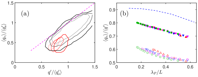
Figure 5: (a) Joint p.d.f. of the r.m.s. velocity and mean vortex mobility. Red lines are for large-vortex turbulence; black are for scrambled positions. Time increases from light to dark, $\omega^{\prime}_{0}t=$ 1.3, 19.6, 52.3, and all the energies are normalised with the mean scrambled energy at each time. Contours contain 99% of the probability mass. (b) Ratio between mobility and r.m.s. velocity. All cases. Symbols as in table 2. Open symbols are unscrambled flows; solid ones are scrambled, and the dashed line is for the Hamiltonian evolution of sets of point vortices with an exponential distribution of circulation. The $\lambda_{P}$ for the point sets is defined using (3).

The second interesting property of the system of large vortices is that they move more slowly that would be expected from the root-mean square velocity of the flow [4]. In particular, if we define the mobility of a vortex core as

$$q_{v}=s^{-1}\left|\int_{s}\boldsymbol{u}{\,\rm{d}}^{2}\boldsymbol{x}\right|$$ (9)

where the integral is taken over the vortex support, it would appear that $\langle q_{v}\rangle$ should be approximately equal to $q^{\prime}$. Figure 5(a) shows that this is not the case. The black contours in the figure are joint probabilities of r.m.s. velocity versus mobility in randomised vortex systems. As could be expected, flows with lower kinetic energy also induce a lower mobility in their cores, but real turbulence, represented by the red contours, not only has a narrower distribution of energy than the scrambled flows, as in figure 4(a), but also lies at the lower edge of the range of mobilities. Considering that the vortices that have been used for the black contours are the same ones used for the red ones, and that the contours enclose 99% of the probability mass in both cases, the vortex distributions in turbulence correspond to very improbable geometric arrangements. For example, the distance between two probability distributions $p_{1}(\boldsymbol{q})$ and $p_{2}(\boldsymbol{q})$, in a parameter space $\boldsymbol{q}$, can be quantified by the Hellinger norm [46], defined by

$$H^{2}(p_{1},p_{2})=\tfrac{1}{2}\int(\sqrt{p_{1}}-\sqrt{p_{2}})^{2}{\,\rm{d}}\boldsymbol{q},$$ (10)

which vanishes for $p_{1}=p_{2}$, and reaches its maximum, $H=1$, for disjoint distributions. In the case of the scrambled and unscrambled distributions in figure 5(a), it varies from $H\approx 0.97$ at early times, when there are many vortices, to $H\approx 0.75$ at the end of the simulations.

Even if the scrambled flows in figure 5(a) tend to have $q_{v}<q^{\prime}$, probably because (9) acts as a filter that smooths the velocity fluctuations, figure 5(b) shows that the low mobility of the turbulence vortices goes beyond this effect. The closed symbols in this figure are the ratio between the mobility and the fluctuation intensity in scrambled flows. It is of the order of 0.75. The open symbols are for turbulence, and, even if the vortices in both cases are the same, and therefore subject to similar filtering effects, the turbulent flows have smaller ratios, of the order of 0.55. Both ratios decrease for decreasing number of vortices, in what is probably another manifestation of the self-exclusion effect in (8). The dashed line in figure 5(b) is computed for Hamiltonian systems of point vortices, which, as we saw above, have very different dynamics from turbulence. In addition, their mobility is a true advection velocity, rather than an average such as (9). Even so, and even if their mobility ratio is closer to unity than in the case of extended vortices, it also decreases with the number of vortices. The simplest explanation, as in (8), is that the self-induced velocity of each vortex is included in $q^{\prime}$ but not in $q_{v}$, and that this difference becomes more important as the number of vortices decreases.

A possibility that needs to be discounted is that the low mobility of the turbulence vortices may be due to geometric jamming, since we saw in figure 1(d) that the inter-vortex distance is of the same order as their diameter. This is not tested by the randomisation of the vortex position in figure 5, because we saw above that this scrambling leads to some vortex overlap, which makes jamming partly irrelevant, but it can be tested by randomly flipping the sign of the vortices, without modifying their vorticity distribution or their shape. This operation respects the vortex geometry and would be as jammed as the original flow field, but the results (not shown) are indistinguishable from those for scrambled positions in figure 5(b).

V The vortex lattice

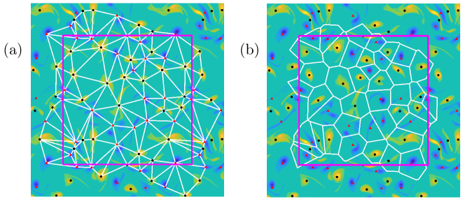
Figure 6: (a) Delaunay triangulation of the lattice of vortex centres. Black dots are positive vortices; red dots are negative. The purple frame is the periodic computational box, and only triangles containing a vertex within the box are plotted. T512. $\omega^{\prime}_{0}t=2.8,\,\lambda_{P}/L=0.30$. (b) The dual Voronoi tessellation of the same field.

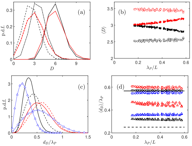
Figure 7: Properties of Delaunay lattice neighbours. (a) P.d.f. of the number of neighbours.   , All neighbours;            , same circulation sign;                   , opposite sign. Red lines are for scrambled vortex positions. T1024a, as in figure 2(a). (b) Mean number of neighbours as function of number of vortices per field. Black symbols are corrotating with the reference vortex. Red ones are counterrotating. All cases. Symbols as in table 2. Open symbols are unscrambled flows; solid ones are scrambled circulations. (c) P.d.f. of the distance between Delaunay neighbours. T2014a, as in figure 2(b). Red lines refer to all neighbours; black lines, to the closest one in each neighbourhood;   , counterrotating with the reference vortex;            , corrotating. Blue lines with symbols used scrambled vortex coordinates. $\circ$, all neighbours; $\scriptstyle\triangle$, closest one. (d) Average distance from a vortex to its Delaunay neighbours. $\circ$, all neighbours; $\scriptstyle\triangle$, closest one. Red symbols only include corrotating vortices; blue are counterrotating, and black include both signs. The two horizontal lines are for scrambled coordinates.   , all neighbours;            , closest one.

We next address what makes the distribution of vortices in turbulent flows atypical. We will focus on the organisation of the centres of gravity of the vortices within their local neighbourhood, since the two previous sections suggest that the vortex distribution over long distances is essentially random.

The conjecture at the end of the §III about the structure of the vortex neighbourhood can be tested by analysing the lattice formed by the vortex centres. Consider the example in figure 6, where the Delaunay triangulation and its associated Voronoi tessellation have been superimposed on the centres of gravity of the vortices within the periodic domain marked by the purple frame [47]. The Delaunay triangulation is the ‘most regular’ triangulation of neighbouring lattice points, and defines lattice neighbourhoods. The Voronoi tessellation is formed by the sets of flow points which are closest to each vortex centre, and defines flow neighbourhoods.

The lattice neighbourhood of a vortex centre can be defined as the set of centres connected to it by a Delaunay edge, and the conjecture in §III can be expressed as that the lattice neighbourhood of a vortex contains, on average, less vortices corrotating with it than counterrotating ones. This would automatically be true for any reasonably homogeneous lattice by the argument in (8), and a second question is whether the observed effect is stronger than could be expected from a random point set. This is tested in figure 7(a), which shows the probability distribution of the degree, $D$ (number of neighbours connected to a given vortex), as well as of the number, $D_{+}$ and $D_{-}$, of corrotating and counterrotating neighbours, respectively. It is known that $\langle D\rangle=6$ for any planar triangulation [47]. This is a topological property, independent of flow structure, but it is clear from figure 7(a) that $\langle D_{-}\rangle>\langle D_{+}\rangle$. The average values of these partial degrees are given in figure 7(b). The open symbols are $D_{+}$ and $D_{-}$; they depend little on the particular case or on the evolution time, and reflect the average loss of one corrotating vortex from each neighbourhood. To test whether this loss is specific to turbulence, the triangulation is repeated after randomising the circulation of the vortices. The results are included as solid symbols in figure 7(b). They show no difference between the two vortex signs at short evolution times, when the flow has many vortices, and drift towards the unscrambled results when the number of vortices decreases at later times. The result of randomising the vortex position instead of the circulation are essentially the same. The origin and magnitude of this drift is the same as in figure 4(d) and in (8).

Figures 7(c,d) display the p.d.f. and mean value of the distance from a vortex to its Delaunay neighbours, $d_{D}$, separated into corrotating and counterrotating ones. The red lines in figure 7(c) and the circles in 7(d) refer to all the neighbours, while the black lines and the triangles refer to the closest one. In both cases they are compared with the result from fields in which the vortex positions are scrambled. The results depend relatively little on the evolution time or on the number of vortices. In all cases, the corrotating neighbours are farther from the reference vortex than the counterrotating ones, in agreement with the ‘tidal capture’ model discussed in §III. This effect is weak in the case of all neighbours, $\langle d_{D}\rangle/\lambda\approx 0.59$ and 0.55, respectively, compared to 0.57 in the randomised case, but much clearer in the case of the closest neighbour, $\langle d_{D}\rangle/\lambda\approx 0.44$, 0.36 and 0.25, respectively. Also striking is that the turbulence p.d.f.s are narrower than the randomised ones, reflecting a more ‘rigid’ geometry that could be interpreted as supporting the description of the lattice as a ‘crystal’. The main difference between turbulence and the randomised field is at short distances, where the vortices do not approach each other beyond $d\approx 0.25\lambda_{P}$, of the order of their diameter (figure 1d). This is again consistent with the tidal model, or even with simple geometric exclusion, and agrees with the result in [4] for nearest neighbours.

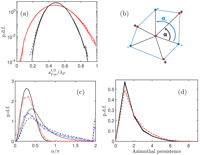
Figure 8: (a) Probability density function of the diameter of the Voronoi tessellae. Black lines are turbulence, and red lines are randomised vortex positions. Each p.d.f is the average of all simulation times.                   , T768;            , T1024;   , T1204a. (b) Sketch of the definition of the angular distance between lattice neighbours, $\alpha$, and between neighbours of a given kind, $\alpha_{\pm}$. (c) P.d.f. of the angular distance among the lattice neighbours to a given vortex.   , all neighbours;            , corrotating with the central vortex;                   , counterrotating;    $\circ$    , all neighbours, with randomised coordinates;    $\scriptstyle\triangle$   , corrotating or counterrotating neighbours, with randomised circulation. T1024a, averaged over all times. (d) P.d.f. of the length of the segments of mutually corrotating vortices in the crowns of immediate neighbours to a given vortex.   , turbulence;            , randomised circulation. The figure includes all the cases in table 2, each one averaged over time, but the results are indistinguishable at the plotting scale.

Figure 8 presents two more indicators of the tendency of turbulent flows to be more organised than random point sets. Figure 8(a) present p.d.f.s of the diameter, $s_{Vor}^{1/2}$, of the individual polygons in Voronoi tessellations, as in figure 6(b). The distribution depends very little on the evolution time and even on the flow parameters, and is shown in the figure averaged over the whole flow decay. It follows from the area-covering property of tessellations, and from (3), that $\langle s_{Vor}\rangle=\lambda_{P}^{2}/4$, or $\langle s_{Vor}^{1/2}\rangle/\lambda_{P}\approx 0.5$. This is true for the centres of gravity of turbulence and for random point sets, but the standard deviation of the turbulence distributions $(0.08\lambda_{P})$ is much narrower than for random sets $(0.125\lambda_{P})$.

The organisation of the vortices in the ‘crown’ that forms the lattice neighbourhood of a given vortex can be characterised by arranging them counterclockwise and measuring the angle $\alpha$ among the consecutive Delaunay edges joining them with the central core (see sketch in figure 8b). Since the average number of lattice neighbours is $\langle D\rangle=6$, one could expect $\langle\alpha\rangle=2\pi/\langle D\rangle=\pi/3$. Empirically, $\langle\alpha\rangle/\pi=0.33\,(1\pm 0.5)$, which is essentially the same as for randomised vortex positions. The situation is different for corrotating or counterrotation neighbours, for which $\langle\alpha_{\pm}\rangle/\pi\approx 2/\langle D_{\pm}\rangle$ also holds, but the standard deviation, $\langle\alpha^{2}_{\pm}\rangle^{1/2}/\langle\alpha_{\pm}\rangle\approx 0.6$, is higher than for the overall angles, and lower than for randomised vortex positions or circulations, $\langle\alpha^{2}_{\pm}\rangle^{1/2}/\langle\alpha_{\pm}\rangle\approx 0.7$. In fact, figure the 8(c) shows that the distribution of the angular distance among corrotating or counterrotating vortices is not just a shifted version of the p.d.f. for all the vortices. Some of the Delaunay neighbours that corrotate (or counterrotate) with respect to their reference vortex are immediate angular neighbours among themselves, and the modal value of the angle distributions is close to the general mode. Their higher mean value is due to a tail of larger angles, required for the total to add to $2\pi$. For example, the corrotating vortices include a substantial spike at $\alpha_{+}=2\pi$, corresponding to crowns with a single corrotating partner.

The sign of the circulation of the vortices within each Delaunay crown is slightly more mixed than would correspond to a random distribution. Figure 8(d) shows the p.d.f. of the length of the segments with similar sign around the crown. For example, the sketch in figure 8(b) is maximally mixed, i.e., its highest azimuthal persistence is one, because there are no contiguous vortices of the same sign. A minimally mixed crown for a set of balanced vortices with the average $D=6$ would have two segments of length three. The dashed lines in figure 8(d) show that a set of random points mostly has contiguous segments of length one or two, with a relatively fat tail extending to full crowns of a single sign. The solid lines in the figure show that the turbulence p.d.f. is slightly more peaked at unity than the random ones, with an average persistence of 1.7. It describes a fairly inhomogeneous crown with less than two consecutive vortices sharing the same sign, although with a slight tendency towards isolated corrotating vortices. The latter is consistent with the already discussed tendency for corrotating vortices to avoid each other.

VI Crystals

Before moving to our final attempt to extract ordered structures from the turbulent flow fields, it is useful to explore whether what we have found up to now can be interpreted as an approximation to stationary crystalline vortex lattices. Two-dimensional vortex crystals are well known [37]. Some of them are stable, and form spontaneously in experiments. Forced two-dimensional turbulence is known to settle to stationary patterns which are partly determined by the forcing and by the boundary conditions [48, 49, 50], although many of the examples do not refer to the Navier–Stokes equations, but to systems such as Bose-Einstein condensates, magnetised plasmas, or superfluids, whose dissipation mechanisms are not exactly those of Navier–Stokes fluids. Beautiful equilibrium vortex polygons have been observed in the polar regions of planetary atmospheres [51].

Most of these examples are regular arrangements of vortices of a single sign in a background of opposite-sign vorticity, but mixed-sign vortex systems with zero overall circulation also exist. The von Kármán vortex street is probably the best-known, and can be generalised to a doubly periodic stationary lattice. Consider the two examples in figure 9(a,b). There are two equilibrium configurations of a double street of point vortices, both of which move with a constant velocity [52, §156]. In the first one, two lines of vortices of opposite sign are staggered, and stacking an infinite number of these ‘staggered’ streets, as in figure 9(a), results in an approximately hexagonal lattice. In the ‘aligned’ equilibrium configuration of two vortex rows, the vortices are vertically aligned with respect to each other, instead of staggered, and they generalise to the ‘cubic’ lattice in figure 9(b).

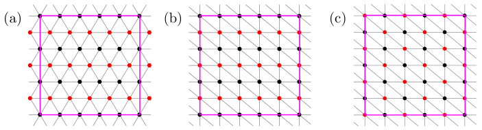
Figure 9: (a) An approximately hexagonal lattice of staggered von Kármán vortex streets. Red dots have positive circulation, and blue ones are negative. (b) A rectangular lattice of aligned streets. (c) A rectangular chequerboard lattice. All these lattices are stationary equilibrium solutions.

While the staggered and aligned von Kármán streets are the only known equilibrium solutions for two lines of vortices of zero total circulation, there are many more doubly infinite equilibrium lattices. Enumerating and analysing them is beyond the scope of this paper, but an example is given in figure 9(c). Note that the three lattices in figure 9 are rotated versions of each other for particular aspect ratios of order unity, but that they are generally distinct, and that they share a structure of alternating layers of vorticity that induce high-velocity streams which could be used as a model for the streams observed in figure 2(c,d).

Figure 10: (a) Normalised interaction energy for the three lattices in figure 9, versus the aspect ratio. Black, staggered von Kármán lattice; red, aligned lattice; blue, chequerboard. The dashed line is a random superposition of between $n_{v}=2$ and 100 Gaussian cores in the computational box. (b) Normalised interaction energy for the point-vortex approximation to the turbulence simulations. Symbols as in table 2.

The interaction energy of these lattices depends on the aspect ratio, defined as $\eta=\Delta y/\Delta x$, where $\Delta x$ is the pitch within each row, and $\Delta y$ is the distance between rows. This energy can be computed analytically in some cases [53], but it is most easily determined by approximating the lattice by a system of compact cores, as in §III, and subtracting the self energy estimated in appendix C. This is done in figure 10(a), where energies are represented normalised per core, and shows that the regular lattices are low-energy states with respect to randomised vortex distributions. The dashed line is the normalised interaction energy for truly random vortex-core systems, computed in the same way, and its small difference from zero is a measure of the accuracy of the estimates in appendix C.

Figure 10(b) contains the energy for the point-vortex approximation to the turbulence simulations in table 2, normalised as in figure 10(a), and shows that turbulence goes a good part of the way to minimising its energy, reaching values comparable to those of infinite regular lattices. It would be nice to relate this low energy to the stability of the different configurations, but energy is not a good indicator of stability. The staggered von Kármán double street is unstable for all aspect ratios except $\eta_{c}\approx 0.28055$, at which it is neutrally stable to linear perturbations [52, 54], but its energy increases monotonically with increasing $\eta$, without any special behaviour at $\eta_{c}$. The lattices in figure 9 have been drawn with an aspect ratio of order $\eta=\tfrac{1}{2}$, suggested by isotropy. Figure 10(a) shows that this is close to the minimum energy configuration for the staggered von Kármán lattice in figure 9(a), but this should not be taken as a stability criterion. It is known that an equilateral triangular lattice is the only stable case for vortex lattices of a single sign [55], but the stability of the mixed cases in figure 9 is unknown.

We are now in a position to discuss in which sense, if any, the statistics of turbulence approximate a lattice such as those in figure 9. Properties such as a uniform Voronoi area (figure 8a) or a constant Delaunay degree (figure 7a) are trivially satisfied by most regular lattices. The angle distribution in figure 8(c) is not different enough from those of randomised vortices to single out a particular lattice, but its narrow distribution around $\pi/3$ rules out the symmetries in figures 9(b,c), which are closer to a bimodal distribution of angles with peaks around $\pi/4$ and $\pi/2$. The azimuthal persistence in figure 8(d), with approximately twice as many isolated vortices of one sign as the number of corrotating pairs, is consistent with any of the layered lattices in figure 9, but not with isolated vortices surrounded by crowns of opposite circulation.

It is interesting that, although we have discussed the imbalance between corrotating and counterrotating neighbours as indications of out-of-equilibrium behaviour, all the equilibrium lattices in figure 9 have twice as many counterrotating Delaunay neighbours as corrotating ones. This is another consequence of the organisation into layers, but is probably not enough to explain the results in figure 7. For one thing, the observed imbalance in the number of neighbours of each class (3.5 to 2.5 in figure 7b), is not close enough to 2 to unambiguously define a regular layered lattice. The ratio between the average distance of the Delaunay neighbours to the distance to the closest one (figure 7d), is more informative. This ratio is fairly close to unity for any of the lattices in figure 9. Even for the square lattices in figures 9(b,c), it is about $d_{av}/d_{min}\approx 1.14$. The average-to-minimum ratio for vortices of all classes in figure 7(d) is approximately 1.8, much closer to the random value, 2.3, than to any regular grid. The set of counterrotating vortices is intermediate between random and regular lattices, $d_{av}/d_{min}\approx 1.54$, but the most ‘regular’ distribution of distances is for the set of vortices corrotating with the centre, for which $d_{av}/d_{min}\approx 1.34$. Moreover, figure 7(d) shows that the mean distance to the central vortex is very similar for the three vortex classes, but that, in agreement with our previous analysis, it is the tight pairs of corrotating vortices that are missing.

In summary, although the statistics presented up to now for the turbulence lattice are consistent with local double layers of counterrotating vortices, they probably cannot be used by themselves as indicators of an ordered lattice over long distances.

VII Crystallography

We finally investigate whether the global vortex organisation can be characterised using Fourier techniques inspired by X-ray crystallography. At first sight, this seems difficult. Fourier analysis of turbulence is similar to powder crystallography, in which diffraction takes place over disparate small crystals with random orientations, and whose typical outcome is only a set of length scales [56]. There are two sources of randomness in the Fourier analysis of turbulent flows. The first one is that individual fields have random orientations, as in powders. The second is that the Fourier transform is an integral over the whole computational box and, since we have seen that non-trivial vortex arrangements probably only extend to local neighbourhoods, the transform also mixes neighbourhoods with random orientations and positions. The randomisation due to the orientation of individual fields is relatively easy to compensate, because we have access to the spectrum of each field. The one due to the global transform requires substituting local expansions for global ones.

In view of the difficulty of identifying global symmetries, we centre this section on the simpler problem of determining whether some specific symmetry applies, on average, to local neighbourhoods of individual vortices. We know from previous sections that the mean distance between vortices is of the order of $\lambda_{P}$, and define neighbourhoods as disks whose radius is some low multiple $R_{P}=\mu\lambda_{P}$. Consider the point-vortex representation of the flow as a set of vortex centres located at $\boldsymbol{x}_{j}$, with circulations $\gamma_{j}$. To study the neighbourhood of the $i$-th vortex, define local polar coordinates, $\boldsymbol{x}_{j}-\boldsymbol{x}_{i}\to(r_{ij},\theta_{ij})$, and construct

$$\widehat{\Gamma}^{[i]}_{n}=\sum_{j}\gamma_{ij}\exp(-{\rm i}n\theta_{ij}),$$ (11)

where $\gamma_{ij}=\gamma_{i}\gamma_{j}/|\gamma_{i}|$, and the sum extends over the vortex centres satisfying $r_{ij}\leq R_{P}$. The effect of the sign factor $(\gamma/|\gamma|)$ in $\gamma_{ij}$ is to classify vortices as co- or counter-rotating with the reference one, $\boldsymbol{x}_{i}$, rather than as positive or negative. Equation (11) is essentially the angular Fourier transform of the projection on the unit circle of the locations of the vortices contained in a neighbourhood disk, and the complex $\widehat{\Gamma}^{[i]}_{n}$ can be written as $|\widehat{\Gamma}^{[i]}_{n}|\exp({\rm i}\psi^{[i]}_{n})$. To overcome the problem of random orientations, we rotate the position of the vortices in each individual neighbourhood so that some specified harmonic, $n_{0}$, is made real and positive,

$$(\widetilde{r}_{ij},\widetilde{\theta}_{ij})\to(r_{ij},\theta_{ij}+\psi^{[i]}_{n_{0}}/n_{0}).$$ (12)

thus rotating other harmonics in (11) to $\widehat{\Gamma}^{[i]}_{n}\exp(-{\rm i}n\psi^{[i]}_{n_{0}}/n_{0})$, and $\widehat{\Gamma}^{[i]}_{n_{0}}$ to $|\widehat{\Gamma}^{[i]}_{n_{0}}|$. Intuitively, this rotation aligns the average position of the cloud of co- (counter-) rotating vortices to preferentially lie in one of the positive (negative) lobes of $\cos(n_{0}\theta_{ij})$, and the resulting ensemble average is a conditional average of the vortex lattice in these aligned coordinates.

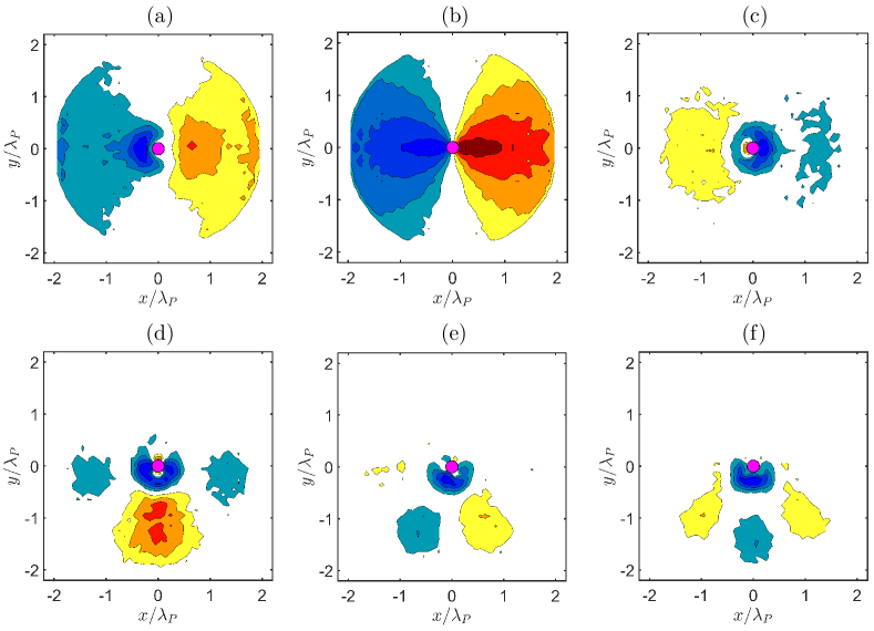
Figure 11: Two-dimensional distribution of vortex positions in oriented flow neighbourhoods, normalised to unit maximum absolute value. T1024a, as in figure 2. $\mu=2$. Contours are $\pm[0.2:0.2:1]$. Red contours are for corrotating vortices, and blue are counterrotating. (a) Turbulence. (b) Randomised positions. (c-f) Turbulence minus randomised. (a-c) $n_{0}=1$. (d) $n_{0}=2$. (e) $n_{0}=3$. (f) $n_{0}=4$. All figures lack the central reference vortex, located at $x=y=0$, that has been indicated by the purple circle whose radius corresponds to the average vortex size in figure 1(d).

An example is figure 11(a), which presents results for an early time in the evolution of T1024a, oriented to $n_{0}=1$, and compares it to a similar flow in which the vortex positions have been randomised (figure 11b). These figures are signed p.d.f.s in which each vortex is counted as $\pm 1$ according to whether it co- or counter-rotates with the central vortex of the neighbourhood. Statistics are compiled over 2000 flow fields, which involve approximately $4\times 10^{6}$ vortices in $2\times 10^{5}$ neighbourhoods. The result is a relatively compact concentration of counterrotating vortices to the left of the figure, $x\approx-0.4\lambda_{P}$, and a more diffuse distribution of corrotating ones to the right. The randomised flow in figure 11(b) does not show the asymmetry between co- and counter-rotating vortices. Its p.d.f simply reflects the structure of the orienting cosine in (11). Figure 11(a) is essentially a directionally unfolded version of the circulation correlation in figure 4(c), but a better way to render it is probably figure 11(c), where the turbulence and randomised distributions have been subtracted. This representation is less affected by artefacts due to the orienting cosine, and becomes more informative when applied to fields oriented to some of the higher harmonics, as in figures 11(d-f). Missing from all the maps in figure 11 is the central reference vortex, corrotating with itself by default, which has been added as a disk at the origin with the radius implied by the average vortex size in figure 1(d). The compact counterrotating cloud present in all figures near the centre is the screening vortex found in the correlations in 4(c). The compact dipole formed by these two vortices appears to be the statistically preferred state of the vortices in turbulence, as already seen in §III, §V and [4].

The more extended vortex clouds farther from the centre, with separations of the order of $1.5\lambda_{P}$, are too far to be considered part of the local neighbourhood (see figure 7c), and belong to the category of the ‘next closest’ vortex. They are of the size of the kinetic-energy streams in figure 2(c,d). An important parameter of the analysis is the multiple $\mu\lambda_{P}$ that determines how many vortices are considered to be part of the local neighbourhood disk. In general, larger neighbourhoods result in a clearer asymmetry, although the signal deteriorates when $R_{P}\gtrsim L/2$ and the conditioning interacts with the periodicity of the numerics, but the outer vortex clouds change little as long as they fit within the analysis disk.

It is probably unwise to read too much in conditional averages, which always retain some influence from the conditioning. The underlying symmetry in figure 11 is dictated by the harmonic used in (12). But the asymmetry between co- and counter-rotating vortices in figures 11(a) and 11(c-f) is a flow property, as shown by the comparison with figure 11(b). So is the separation among the different vortex clouds in the figures, and it is tempting to see in figure 11 fragments of the regular grids in figure 9. Note that the distances involved are rather large. We saw in §II that a disk of radius $\lambda_{P}$ approximately contains 15 vortices. The analysis disk used in figure 11, with $\mu=2$, therefore represents the organisation of about 60 vortices.

VIII Conclusions

The results in this paper describe how decaying two-dimensional turbulence spontaneously organises into a low-energy lattice of large vortices that is substantially more ordered than a random vortex distribution, and evolves more slowly than other parts of the flow, but which is neither fully ordered over long distances, nor stationary. It contains most of the kinetic energy of the flow, and could perhaps be described as a vortex ‘liquid’, rather than a gas or a crystalline solid. We may call it a ‘stochastic crystal’.

We have shown that what could be called the ‘latent heat’ of randomisation is not an issue in turbulence decay. The vortices in the flow never explore the randomised states, and they approximately conserve energy by staying within a very restricted fraction of the configuration space of vortex positions. If we consider the process of vortex amalgamation during decay as a late stage of the condensation of the flow vorticity into compact cores, vortex formation and order generation are parts of the same process.

We have seen that maintaining a low relative energy of the vortex lattice requires mutual screening of the far field of the vortex-induced velocity, but that this is not implemented by attracting vortices of opposite sign to surround each other, as in electrostatics, but by preferentially absorbing vortices of the same sign, in a process akin to tidal disruption in strong gravitational fields.

The resulting vortex lattices are not organised enough to be considered equilibrium solutions, but they are shown by various geometric analyses to locally approximate double vortex layers, which move slowly and could perhaps be related to fixed points of the dynamical system representing the flow. However, the equilibrium is constantly disrupted in decaying turbulence by the capture process mentioned above, which ensures that the neighbourhood of each vortex contains on average one more counterrotating vortex than corrotating ones.

One of the referees called attention to the possible dependence of the above results on the initial conditions. This is an important issue in transient or decaying flows. It is known, for example, that the long-term behaviour of the large scales in decaying three-dimensional turbulence depends on the small-wavenumber slope of the initial energy spectrum, $E_{qq}\sim k^{\zeta}$, and that $\zeta=2$ and $\zeta=4$ are distinguished values that tend to persist during the decay (see [35] and references therein). This persistence is not preserved in two dimensions, because the inverse cascade continuously pumps energy into the large scales, where it ‘condenses’ and destroys any pre-existing spectral structure [25]. All our simulations use $\zeta=-1/2$ [4], but the shorter spectral peak of case T1024a was specifically introduced to explore the effect of different initial spectra, and a few cursory experiments were run with $\zeta=-2$ to $\zeta=4$ for the same purpose. The main effect of $\zeta$ is to change the rate at which the large scales condense, which also modifies the balance between disordered small vortices and ordered large ones. Very ‘peaked’ spectra $(\zeta>0)$ introduce an initial family of vortices of approximately uniform size, which does not completely disappears by the time that the rest of the energy has condensed. Tests like the distribution of Voronoi areas in figure 8(a) suggest that the large vortices in these flows are even more organised than in the cases discussed in the present paper. For an initially uniform enstrophy spectrum $(\zeta=-2)$, the flow is condensed from the beginning, and vortex families do not have time to form. The elucidation of the full range of possible behaviours would unfortunately extend this paper beyond any reasonable length, and has not been attempted. The present results should be seen as evidence of the spontaneous segregation of a relatively organised subset of large vortices from an initial condition in which vortices have widely scattered (power law) sizes and circulations.

Whether any of the mechanisms described here can be generalised to three-dimensional flows is under investigation, but unknown at present.

Appendix A Point-vortex simulations

There are two compact vortex approximations used for comparison in the text. This appendix describes them, and their numerical issues.

A.1 Gaussian cores

The first approximation, used in §III–VI, substitutes the precomputed turbulence vortices by Gaussian cores,

$$\omega_{g}(\boldsymbol{x})=(\gamma/\pi R^{2})\exp(-|\boldsymbol{x}-\boldsymbol{x}_{cog}|^{2}/R^{2}),$$ (13)

where $\gamma$ is the circulation of the turbulence vortex being approximated, and the centre of gravity is defined over the vortex support, $s$, as

$$\boldsymbol{x}_{cog}=s^{-1}\int_{s}\boldsymbol{x}\,\omega(\boldsymbol{x}){\,\rm{d}}^{2}\boldsymbol{x},$$ (14)

The core radius is arbitrarily set to $R/L=10^{-2}$, except for some convergence tests at $R/L=2.5\times 10^{-3}$, and the core area, when needed, is defined as $s_{g}=\pi R^{2}$.

There is no dynamics in this operation, which represents an existing flow field. The cores are added to an empty $1024^{2}$ numerical grid, a uniform background vorticity is added to zero the overall circulation, and flow quantities of this synthetic field are computed in the usual manner.

The kinetic energy of the regular lattices in §VI are also computed using this procedure.

A.2 Hamiltonian point vortices

In contrast to the postprocessing operation just described, some simulations were run for Hamiltonian systems of point vortices. Defining a complex variable, $z=x+{\rm i}y$, each vortex satisfies

$${\rm{d}}_{t}\overline{z}_{j}=\overline{w}_{j}=u_{j}-{\rm i}v_{j}=\sum_{k\neq j}\frac{\gamma_{k}}{2\pi{\rm i}(z_{j}-z_{k})},$$ (15)

where $\gamma_{k}$ is the circulation of the individual vortices, and the overline denotes complex conjugation. For a doubly periodic flow in $L\times L$, the right-hand side is substituted by [52]

$$\overline{w}_{j}=\frac{1}{2{\rm i}L}\sum_{k}\gamma_{k}\sum_{m^{\prime}=\infty}^{\infty}\cot\left(\frac{\pi(z_{j}-z_{k})}{L}+{\rm i}m\pi\right),$$ (16)

where the inner sum includes $m=0$ except for $k=j$. In practice, this inner series can be truncated to $m\leq 2$. The system (16) is integrated with a second-order Runge-Kutta, which is formally symplectic for uniform time step, $\Delta t$ [57]. The spatial resolution is determined by this time step. The critical case is when two corrotating vortices get closer than a distance $\ell$, in which case they should rotate around each other with velocity $|w|=\gamma/2\pi\ell$. Accuracy requires that $|w|\Delta t\ll\ell$, or $\ell\gg(\gamma\Delta t/2\pi)^{1/2}$. The accuracy constraint is laxer for counterrotating pairs, which tend to translate in a straight line. For shorter distances, corrotating and counterrotating pairs behave different for numerical reasons, and there is an apparent correlation dip reminiscent of figure 4(c). This was tested by changing the time step by a factor of 4, so that $\ell/\lambda_{P}=0.05-0.2$, and became the reason why T1024a was rerun at a twice-shorter time step, without any effect.

Appendix B Vortex overlap

Consider sets of $N$ circular vortices, of uniform diameter $R$, in a box of area $L^{2}$. Two vortices intersect if their centres are at a distance $h<2R$, and the relevant parameter is $\sigma=h/2R\in(0,1)$. The area of their intersection is

$$\Delta S/2R^{2}=\arccos(\sigma)-\sigma(1-\sigma^{2})^{1/2}.$$ (17)

The probability density of the centre of a vortex being at a distance $h$ from another one is $2\pi h/L^{2}$, so that the average intersection area is

$$\langle\Delta S_{1}\rangle=\int_{0}^{1}p(\sigma)\Delta S{\,\rm{d}}\sigma=\frac{16\pi R^{4}}{L^{2}}\int_{0}^{1}\sigma\left[\arccos(\sigma)-\sigma(1-\sigma^{2})^{1/2}\right]{\,\rm{d}}\sigma=\frac{\pi^{2}R^{4}}{L^{2}}.$$ (18)

Since the total number of possible vortex pairs is $N(N-1)/2$, and the total vortex area in $\pi NR^{2}$, the relative area fraction of the intersections is

$$\langle\Delta S_{N}\rangle/S_{N}=(N-1)\pi R^{2}/2L^{2}\approx 0.5S_{N}/L^{2}.$$ (19)

The experimental factor is closer to 0.45, but the relation holds very well, particularly for the circular Gaussian cores.

Appendix C The vortex energy

Consider a system of $n_{v}$ compact vortices in a doubly periodic box of side $L$, assumed to be of radius $R\ll L$ and divided into equal numbers of positive and negative circulation, $\pm\gamma$. A rough estimation of the r.m.s. velocity fluctuations that they generate follows from assuming their induced velocities to be independent variables whose individual variance is the average

$$q_{1}^{\prime 2}=\frac{1}{L^{2}}\,\int_{L^{2}}\left(\frac{\gamma}{2\pi|\boldsymbol{x}|}\right)^{2}{\,\rm{d}}^{2}\boldsymbol{x}\approx\frac{1}{L^{2}}\,\int_{R}^{\ell_{0}}\left(\frac{\gamma}{2\pi r}\right)^{2}2\pi r{\,\rm{d}}r=\frac{\gamma^{2}}{2\pi L^{2}}\,\log(\ell_{0}/R),$$ (20)

where $\ell_{0}$ is an outer scale beyond which the $1/r$ velocity law ceases to apply. The expected velocity variance, or kinetic energy, due to $n_{v}$ cores is of the order of

$$q^{\prime 2}=q^{\prime 2}_{1}n_{v}\approx\frac{\gamma^{2}n_{v}}{2\pi L^{2}}\log(\ell_{0}/R).$$ (21)

Note that the assumption in this equation, in the notation of the body of the paper, is that ramdomised vortices only have self energy. If we similarly estimate the mean enstrophy as

$$\omega^{\prime 2}\approx(\gamma/R^{2})^{2}n_{v}(R/L)^{2},$$ (22)

we obtain

$$q^{\prime 2}/(\omega^{\prime 2}R^{2})\sim\log(\ell_{0}/R).$$ (23)

For regular lattices such as those in §VI, $\ell_{0}=2(\Delta_{1}\Delta_{2})^{1/2}/\pi$, where the $\Delta_{j}$ are the lengths of the two vectors that define the lattice cell [53]. For a random superposition of vortices in a periodic box, this becomes $\ell_{0}=2L/\pi$, and the logarithmic correction in figure 4(b) applies. On the other hand, if the velocity is screened beyond distances proportional to $R$, the correction disappears.