Analysis of a 3-RUU Parallel Manipulator

Abstract

The aim of this paper is to give a detailed examination of the input and output singularities of a 3-RUU parallel manipulator in the translational operation mode. This task is achieved by using algebraic constraint equations. For this type of manipulator a complete workspace representation in Study coordinates is presented after elimination of the input parameters. Both, input and output singularities are mapped into a Study subspace as well as into the joint space. Therewith a detailed singularity investigation of the translational operation mode of a 3-RUU parallel manipulator is provided. This paper is an extended version of a previous publication. The addendum comprises the discovery of a possible transition between two operation modes as well as a self motion and an examination of another component of the output singularity surface, most of them for arbitrary design parameters.

1 Introduction

There are many different approaches to perform the kinematic analysis of parallel manipulators (PM). More recently dual quaternions have been used to describe the group of Euclidean displacements $\mathrm{SE}(3)$. Together with the use of Study’s kinematic mapping they have proven to be very successful to obtain information about the global behavior of parallel manipulators. The aims of this kinematic analysis are to derive algebraic constraint equations, to solve the direct and inverse kinematics, to describe the complete workspace, operation modes and all singularities (e.g. [9]).

There are numerous papers investigating workspace and singularities of parallel manipulators especially of the Stewart-Gough platform e.g. by Dasgupta and T.S. Mruthyunjaya [7], Borràs et al. [3] or Nawratil [8, 10]. Also closely related manipulators were already investigated for example the 4-RUU in Amine et al. [1].

There are also numerous papers on lower degree of freedom parallel manipulators, most of them use vector loop equations or screw theory for the kinematic analysis. Analyzing the global kinematics of lower degree of freedom parallel manipulators using algebraic constraint equations one can explain the overall kinematic behavior, e.g. determining different operation modes, transition between the operation modes and all singularities of the manipulator (for example [11]).

This paper is an extension of [13] which used results of  [12] to provide an even more detailed singularity analysis of the translational operation mode of a 3-RUU parallel manipulator. Furthermore, an algebraic representation of the workspace is derived, which might prove to be very useful in several kinematic tasks like path planning. To the best of the authors knowledge this is the first non-trivial lower degree of freedom PM known with an input parameter free description of the workspace. Section 2 recalls the manipulator’s architecture and the algebraic constraint equations that describe its motion capabilities. Section 3 shows the algorithm to derive the workspace equations, which are only displayed for the translational mode in this paper due to their length. In Section 4 a thorough singularity analysis of the translational mode is given comprising a detailed description of input and output singularities in the kinematic image space (Study space) as well as in the joint space. The main part of the extension comprises an investigation on constraint singularities and possible transition between operation modes. Additionally, a profound examination of the output singularities results in the discovery of a self motion as well as a new component of the singularity surface. In contrast to [13], most of the results are derived for arbitrary design parameters. The last section concludes the results.

2 Manipulator Architecture and Constraint Equations

As there is a detailed explanation of the 3-RUU parallel manipulator’s architecture in Stigger et al. [12] its architecture is only briefly explained. The manipulator consists of three identical RUU-limbs (Fig. 1).

\begin{overpic}[scale={.38}]{Figures/3ruu-canonical-leg_1} \put(285.0,65.0){$\Sigma_{0}$} \put(70.0,40.0){$\Sigma_{1}$} \put(230.0,55.0){$a_{1}$} \put(120.0,40.0){$a_{3}$} \put(220.0,30.0){$x_{0}$} \put(300.0,25.0){$y_{0}$} \put(280.0,105.0){$z_{0}$} \put(5.0,5.0){$x_{1}$} \put(85.0,0.0){$y_{1}$} \put(65.0,80.0){$z_{1}$} \end{overpic}

Figure 1: A RUU limb

Each of them comprises three joints, an actuated revolute (R) and two passive universal (U) joints. Each vertex of the equilateral base triangle is connected via an RUU limb with a vertex of the equilateral moving platform triangle. The first and the last axis in each limb are tangent to the circum-circles of base and moving triangular platform, respectively (Fig. 2). The geometric design of each limb is described with Denavit-Hartenberg (DH) parameters [6].

\begin{overpic}[scale={.38}]{Figures/3ruu} \put(188.0,146.0){$\Sigma_{1}$} \put(188.0,63.0){$\Sigma_{0}$} \put(28.0,96.0){$a_{1}$} \put(50.0,128.0){$a_{3}$} \put(195.0,180.0){$z_{1}$} \put(150.0,155.0){$x_{1}$} \put(175.0,145.0){$y_{1}$} \put(150.0,78.0){$x_{0}$} \put(173.0,65.0){$y_{0}$} \put(192.0,100.0){$z_{0}$} \end{overpic}

Figure 2: 3-RUU parallel manipulator

2.1 Constraint Equations

For the workspace and singularity analysis algebraic constraint equations of the 3-RUU chains are convenient. These equations have been derived with different methods in [12]. Therefore, the lengthy derivation of the constraint equations is omitted here and the reader is referred to this paper. The constraint equations describing a canonical RUU limb in Euclidean space with respect to proper coordinate systems $\Sigma_{0}$, $\Sigma_{1}$ (Fig. 1) are

$$f_{1}: \left(\left(x_{{0}}x_{{1}}-x_{{2}}x_{{3}}\right)({t}^{2}-1)-\left(2x_{{0}}x_{{2}}+2x_{{1}}x_{{3}}\right)t\right)a_{{1}}+2\left({t}^{2}+1\right)\left(x_{{0}}y_{{0}}+x_{{3}}y_{{3}}\right)=0,$$

$$f_{2}: -\left({x_{{0}}}^{2}+{x_{{1}}}^{2}+{x_{{2}}}^{2}+{x_{{3}}}^{2}\right)\left({t}^{2}+1\right){a_{{1}}}^{2}+\left(4\left(x_{{0}}y_{{1}}-x_{{1}}y_{{0}}+x_{{2}}y_{{3}}-x_{{3}}y_{{2}}\right){t}^{2}\right.$$

$$+8\left(-x_{{0}}y_{{2}}+x_{{1}}y_{{3}}+x_{{2}}y_{{0}}-x_{{3}}y_{{1}}\right)t\left.-4\left(x_{{0}}y_{{1}}-x_{{1}}y_{{0}}+x_{{2}}y_{{3}}-x_{{3}}y_{{2}}\right)\right)a_{{1}}$$

$$+\left(\left({x_{{0}}}^{2}+{x_{{1}}}^{2}+{x_{{2}}}^{2}+{x_{{3}}}^{2}\right){a_{{3}}}^{2}-\,4\left({y_{{0}}}^{2}+{y_{{1}}}^{2}+{y_{{2}}}^{2}+{y_{{3}}}^{2}\right)\right)\left({t}^{2}+1\right)=0.$$ (1)

The parameters $a_{1}$ and $a_{3}$ denote the leg lengths. Further, $x_{i}$, $y_{i}$ for $i=0$, $1$, $2$, $3$ are the coordinates (Study parameters) in a seven-dimensional projective space $\mathbb{P}^{7}$, also called kinematic image space or Study space. They determine the possible poses of the moving coordinate system $\Sigma_{1}$ with respect to the base system $\Sigma_{0}$. The parameter $t$ is the algebraic value, using tangent half-angle substitution, of the input angle of the first revolute joint. From the canonical constraint equations in Eq. (2.1), the general ones are found by applying transformations that move the limbs from the origin of the base system to their appropriate positions on the manipulator. Mathematically, they are obtained by performing transformations of the $x_{i}$, $y_{i}$ coordinates in $\mathbb{P}^{7}$ that are applied to the set of canonical constraint equations. It is important to note that these transformations do not change the degree of the constraint equations [9]. For each limb the appropriate transformations are applied to $f_{1}$ and $f_{2}$ which move each of the limbs to the respective corners of the base triangle (Fig. 2). Additionally, the input parameter $t$ is substituted with $t_{1}$, $t_{2}$ and $t_{3}$, respectively. The radii of the base and moving platforms circum-circles are denoted by $r_{0}$ and $r_{1}$, respectively. In total this results in six general constraint equations $g_{1},\ldots,g_{6}$. Together with the equation of the Study quadric $g_{7}:x_{0}y_{0}+x_{1}y_{1}+x_{2}y_{2}+x_{3}y_{3}=0$ and a normalization condition $g_{8}:x_{0}^{2}+x_{1}^{2}+x_{2}^{2}+x_{3}^{2}=1$ these equations yield a complete kinematic description of the manipulator, involving the three input parameters $t_{1}$, $t_{2}$ and $t_{3}$. Therefore the set ${\cal W}=\{g_{1},\ldots,g_{8}\}$ forms a three parameter system of constraint equations in the Study parameters which define the three dimensional constraint variety in $\mathbb{R}^{11}$.

3 Workspace Description

For path planning it would be convenient to have a system of equations without the input parameters describing the workspace only in image space coordinates. Inspection of the constraint equations shows that they are only pairwise dependent on the same input parameter: $g_{1}$ and $g_{2}$ for example depend only on $t_{1}$. Eliminating $t_{1}$ via computing the resultant of $g_{1}$ and $g_{2}$ yields an equation depending on the Study parameters only. Using the same procedure on $g_{3}$, $g_{4}$ thereby eliminating $t_{2}$ as well as on $g_{5}$, $g_{6}$ eliminating $t_{3}$, three equations $g_{12}$, $g_{34}$, $g_{56}$ are obtained. These three resulting equations are independent of the input parameters and yield together with $g_{7}$ and $g_{8}$ a suitable description of the workspace for path planning. As the computation is straightforward from the set of equations (2.1) and due to their length the three equations $g_{12}$, $g_{34}$ and $g_{56}$ are not shown. But it is easy to show that the whole translational three-space given by

$${x_{0}}=1,\leavevmode\nobreak\ {x_{1}}={x_{2}}={x_{3}}=y_{0}=0$$ (2)

lies in the workspace, a fact that confirms once more that the manipulator has a translational operation mode denoted by $O_{1}$, although it is not the only mode. In order to determine all operation modes, one needs to analyze the irreducible components of the workspace variety. Unfortunately the equations are too complicated to perform a primary decomposition. However, the open source software Bertini${}^{\text{TM}}$ [2], a numerical algebraic geometry software for solving polynomial systems, can be used to gain an idea about the potential number of the components as well as their particular dimension and degree. As Bertini${}^{\text{TM}}$ is a numerical software, real values for the leg lengths and the radii of the circum-circles of the base and moving triangle have to be set. Running Bertini${}^{\text{TM}}$ for different designs resulted in equivalent outputs. In the following, the design

$$a_{1}=3,\leavevmode\nobreak\ a_{3}=5,\leavevmode\nobreak\ r_{0}=11,\leavevmode\nobreak\ r_{1}=7,$$ (3)

is used as an example, Fig. 2. According to [2], results of this software hold true with very high probability depending on the numerical error. With the equations $g_{12}$, $g_{34}$, $g_{56}$, $g_{7}$, $g_{8}$ as input Bertini${}^{\text{TM}}$ classifies three components, each of dimension three. Besides the translational three-space (2) there is another linear component. Although Bertini${}^{\text{TM}}$ does not provide an algebraic description of the detected components, the knowledge about their dimension and degree restricts the set of potential candidates and one finds the second linear component to be given by

$${x_{3}}=1,\leavevmode\nobreak\ {x_{0}}={x_{1}}={x_{2}}=y_{3}=0.$$ (4)

This is again a three-space in $\mathbb{P}^{7}$ denoted by $O_{2}$. It describes a “twisted translational operation mode”, that is a translational mode where the moving platform is rotated by a half turn about the $z$-axis with respect to the base platform. Again, it is easy to verify, that this result is independent of the chosen design parameters. According to the output of Bertini${}^{\text{TM}}$, there exists a third component, denoted by $O_{3}$, of degree $944$ which suggests that it is a rather difficult task to compute generators of a defining ideal as well as determining whether this component is irreducible.

4 Singularity Analysis of the Translational Operation Mode

Singularities in parallel mechanisms can occur either because one limb or the platform itself is in a singular position. Furthermore, both can take place at the same time meaning that a limb and the platform are in singular positions. In Section 3 operation modes of the 3-RUU are identified. Below, a detailed analysis and characterization of the input and output singularities of the translational operation mode $O_{1}$ will be given. In contrast to constraint singularities, where the tangent space gains dimensions, these singularities are points at which the tangent space contains elements independent of the input or Study parameters, respectively. The tangent space at a point is the kernel of the Jacobian $\mathbf{J}=[\mathbf{J_{o}},\mathbf{J_{i}}]$ evaluated at this point. Here $\mathbf{J_{o}}$ is the derivative of the constraint equations with respect to the Study parameters and $\mathbf{J_{i}}$ is the derivative with respect to the input parameters. The subscript $o$ refers to output and $i$ refers to input. In the following input and output singularities for the translational mode will be discussed separately in joint space as well as in the kinematic image space. Provided the conditions (2) hold, $g_{1}$, $g_{3}$, $g_{5}$, $g_{7}$ and $g_{8}$ become trivial (meaning here that the left hand sides of these equations vanish, yielding $0=0$). Hence the system $\cal W$ reduces to a system of three equations

$$g_{2}: \left({{a_{1}}}^{2}-{{a_{3}}}^{2}+(r_{0}-r_{1})^{2}+4(y_{1}^{2}+y_{2}^{2}+y_{3}^{2}-a_{1}y_{3}+r_{0}y_{1}-r_{1}y_{1})\right){{t_{1}}}^{2}$$

$$+4a_{1}\left({r_{0}}-{r_{1}}+2{y_{1}}\right){t_{1}}$$

$$+(r_{0}-r_{1})^{2}+4(y_{1}^{2}+y_{2}^{2}+y_{3}^{2}+a_{1}y_{3}+r_{0}y_{1}-r_{1}y_{1})+a_{1}^{2}-a_{3}^{2}=0,$$

$$g_{4}: \left(2(r_{0}-r_{1})\left(\sqrt{3}y_{2}-y_{1}\right)+(r_{0}-r_{1})^{2}+4(y_{1}^{2}+y_{2}^{2}+y_{3}^{2}-a_{1}y_{3})+a_{1}^{2}-a_{3}^{2}\right){{t_{2}}}^{2}$$

$$+4a_{1}\left(\sqrt{3}y_{2}+r_{0}-r_{1}-y_{1}\right){t_{2}}$$

$$+2(r_{0}-r_{1})(\sqrt{3}y_{2}-y_{1})+(r_{0}-r_{1})^{2}+4(y_{1}^{2}+y_{2}^{2}+y_{3}^{2}+a_{1}y_{3})+a_{1}^{2}-a_{3}^{2}=0,$$

$$g_{6}: \left(-2(r_{0}-r_{1})(\sqrt{3}y_{2}+y_{1})+(r_{0}-r_{1})^{2}+4(y_{1}^{2}+y_{2}^{2}+y_{3}^{2}-a_{1}y_{3})+a_{1}^{2}-a_{3}^{2}\right){{t_{3}}}^{2}$$

$$+4a_{1}\left(-\sqrt{3}y_{2}+r_{0}-r_{1}-y_{1}\right)t_{3}$$

$$-2(r_{0}-r_{1})(\sqrt{3}y_{2}+y_{1})+(r_{0}-r_{1})^{2}+4(y_{1}^{2}+y_{2}^{2}+y_{3}^{2}+a_{1}y_{3})+a_{1}^{2}-a_{3}^{2}=0.$$

This system of equations is denoted by $\cal{W_{T}}$ and describes the translational operation mode for arbitrary design. Note that in order to cover all singular points on the variety defined by $\cal{W_{T}}$, one still has to compute the Jacobian of the system $\cal{W}$ before substituting the conditions for the translational operation mode in Eq. (2) into $\mathbf{J}$.

4.1 Input Singularities

Following Gosselin and Angeles [5], input singularities occur when $\mathbf{J_{i}}$ is rank deficient. As there are two general constraints per limb plus the Study condition $g_{7}$ and the normalization condition $g_{8}$, the system $\cal W$ consists of eight equations. On the other hand there are only three input variables. The resulting $8\times 3$ Jacobian matrix is obviously not square. The algebraic condition for rank deficiency is that all $3\times 3$ sub-determinants vanish. When the conditions for the translational mode (2) are substituted into the system of sub-determinants, all equations but one become trivial. The only remaining one factors into $p_{1}\cdot p_{2}\cdot p_{3}=0$ with

$$p_{1}: \left({{a_{1}}}^{2}-{{a_{3}}}^{2}+(r_{0}-r_{1})^{2}+4(y_{1}^{2}+y_{2}^{2}+y_{3}^{2}-a_{1}y_{3}+r_{0}y_{1}-r_{1}y_{1})\right){{t_{1}}}$$ (5)

$$+2a_{1}\left({r_{0}}-{r_{1}}+2{y_{1}}\right),$$

$$p_{2}: \left(2(r_{0}-r_{1})\left(\sqrt{3}y_{2}-y_{1}\right)+(r_{0}-r_{1})^{2}+4(y_{1}^{2}+y_{2}^{2}+y_{3}^{2}-a_{1}y_{3})+a_{1}^{2}-a_{3}^{2}\right){{t_{2}}}$$

$$+2a_{1}\left(\sqrt{3}y_{2}+r_{0}-r_{1}-y_{1}\right),$$

$$p_{3}: \left(-2(r_{0}-r_{1})(\sqrt{3}y_{2}+y_{1})+(r_{0}-r_{1})^{2}+4(y_{1}^{2}+y_{2}^{2}+y_{3}^{2}-a_{1}y_{3})+a_{1}^{2}-a_{3}^{2}\right){{t_{3}}}$$

$$+2a_{1}\left(-\sqrt{3}y_{2}+r_{0}-r_{1}-y_{1}\right).$$

Each factor is related to one limb of the mechanism. Since it is sufficient that one of the three factors vanishes in order to satisfy the singularity condition only the first of the factors is discussed here in detail. The other ones can be treated analogously. As $p_{1}$ in Eq. (5) is linear in $t_{1}$, it has the unique root at

$$t_{1}=\frac{2{a_{1}}\left({r_{1}}-{r_{0}}-2{y_{1}}\right)}{\left({{a_{1}}}^{2}-{{a_{3}}}^{2}+(r_{0}-r_{1})^{2}+4(y_{1}^{2}+y_{2}^{2}+y_{3}^{2}-a_{1}y_{3}+r_{0}y_{1}-r_{1}y_{1})\right)},$$ (6)

provided that the leading coefficient of $p_{1}$ with respect to $t_{1}$, i.e. the denominator in (6), does not vanish. Substituting $t_{1}$ from Eq. (6) into the system $\cal W_{T}$, its first equation simplifies to

$$0= \leavevmode\nobreak\ {{a_{1}}}^{4}-2{{a_{3}}}^{2}{{a_{1}}}^{2}-2{{r_{0}}}^{2}{{a_{1}}}^{2}+4{r_{0}}{r_{1}}{{a_{1}}}^{2}-8{r_{0}}{{a_{1}}}^{2}{y_{1}}-2{{r_{1}}}^{2}{{a_{1}}}^{2}+8{r_{1}}{{a_{1}}}^{2}{y_{1}}$$ (7)

$$-8{{a_{1}}}^{2}{{y_{1}}}^{2}+8{{a_{1}}}^{2}{{y_{2}}}^{2}-8{{a_{1}}}^{2}{{y_{3}}}^{2}+{{a_{3}}}^{4}-2{{a_{3}}}^{2}{{r_{0}}}^{2}+4{{a_{3}}}^{2}{r_{0}}{r_{1}}-8{{a_{3}}}^{2}{r_{0}}{y_{1}}$$

$$-2{{a_{3}}}^{2}{{r_{1}}}^{2}+8{{a_{3}}}^{2}{r_{1}}{y_{1}}-8{{a_{3}}}^{2}{{y_{1}}}^{2}-8{{a_{3}}}^{2}{{y_{2}}}^{2}-8{{a_{3}}}^{2}{{y_{3}}}^{2}+{{r_{0}}}^{4}-4{{r_{0}}}^{3}{r_{1}}$$

$$+8{{r_{0}}}^{3}{y_{1}}+6{{r_{0}}}^{2}{{r_{1}}}^{2}-24{{r_{0}}}^{2}{r_{1}}{y_{1}}+24{{r_{0}}}^{2}{{y_{1}}}^{2}+8{{r_{0}}}^{2}{{y_{2}}}^{2}+8{{r_{0}}}^{2}{{y_{3}}}^{2}-4{r_{0}}{{r_{1}}}^{3}$$

$$+24{r_{0}}{{r_{1}}}^{2}{y_{1}}-48{r_{0}}{r_{1}}{{y_{1}}}^{2}-16{r_{0}}{r_{1}}{{y_{2}}}^{2}-16{r_{0}}{r_{1}}{{y_{3}}}^{2}+32{r_{0}}{{y_{1}}}^{3}+32{r_{0}}{y_{1}}{{y_{2}}}^{2}$$

$$+32{r_{0}}{y_{1}}{{y_{3}}}^{2}+{{r_{1}}}^{4}-8{{r_{1}}}^{3}{y_{1}}+24{{r_{1}}}^{2}{{y_{1}}}^{2}+8{{r_{1}}}^{2}{{y_{2}}}^{2}+8{{r_{1}}}^{2}{{y_{3}}}^{2}-32{r_{1}}{{y_{1}}}^{3}$$

$$-32{r_{1}}{y_{1}}{{y_{2}}}^{2}-32{r_{1}}{y_{1}}{{y_{3}}}^{2}+16{{y_{1}}}^{4}+32{{y_{1}}}^{2}{{y_{2}}}^{2}+32{{y_{1}}}^{2}{{y_{3}}}^{2}+16{{y_{2}}}^{4}$$

$$+32{{y_{2}}}^{2}{{y_{3}}}^{2}+16{{y_{3}}}^{4}$$

Since the other two equations of $\cal W_{T}$ involve only $t_{2}$ and $t_{3}$, respectively, one always finds values for these input parameters such that these equations hold for $y_{1}$, $y_{2}$, $y_{3}$ fulfilling Eq. (7). It remains to discuss the case when the leading coefficient of $p_{1}$ with respect to $t_{1}$ is zero, i.e.

$${{a_{1}}}^{2}-4{a_{1}}{y_{3}}-{{a_{3}}}^{2}+{{r_{0}}}^{2}-2{r_{0}}{r_{1}}+4{r_{0}}{y_{1}}+{{r_{1}}}^{2}-4{r_{1}}{y_{1}}+4{{y_{1}}}^{2}+4{{y_{2}}}^{2}+4{{y_{3}}}^{2}=0$$ (8)

In this case, the constant term of $p_{1}$ needs to be zero as well, that is $y_{1}=(r_{1}-r_{0})/2$. Substituting this condition into $\cal W_{T}$ and simplifying with (8), one obtains the further condition $y_{3}=0$. Moreover one gets $y_{2}=\pm\sqrt{(a_{3}^{2}-a_{1}^{2})/4}$ via substituting $y_{1}=(r_{1}-r_{0})/2$ and $y_{3}=0$ into Eq. (8). However the two points $\left((r_{1}-r_{0})/2,\pm\sqrt{(a_{3}^{2}-a_{1}^{2})/4},0\right)$ already lie on the surface defined by Eq. (7), thus this equation together with the system $\cal{W_{T}}$ yields the singularity surface in the kinematic image space related to the first limb. It has the following interpretation: when a pose of the manipulator in the translational operation mode is chosen such that Eq. (7) is fulfilled, then the first limb is either stretched out or folded. The surface can be visualized in the three dimensional Study subspace spanned by $y_{1}$, $y_{2}$, $y_{3}$ representing all translations. Fig. 3 shows the input singularity surface for the first limb of the 3-RUU PM with the design parameters in Eq. (3). An easy computation shows that it is a torus.

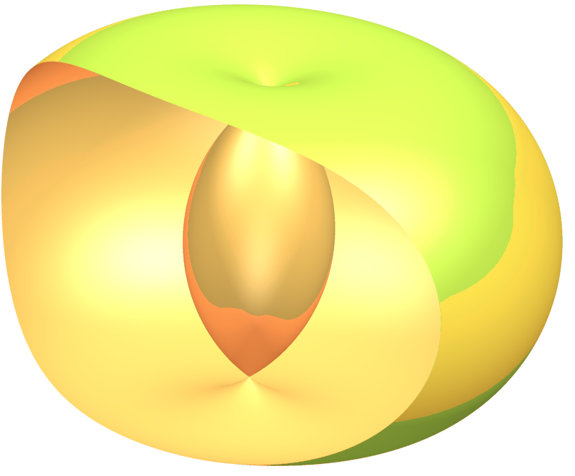
Figure 3: Spindle torus as input singularity surface for one limb in Study space

The other two factors in Eq. (5) yield also tori which are rotated by $\pm 120^{\circ}$ about the $y_{3}$-axis. All three surfaces have two points in common. These points correspond to poses where all three limbs are singular. Intersection curves of a pair of tori correspond to poses where two limbs are singular.

For practical control purposes it would be convenient to have a representation of the input singularities in joint space, as to avoid these inputs during operation. In order to simplify computations and display the results the design parameters in Eq. (3) are set. However, the procedure below can be performed for any design. A condition for the first limb to be in a singular position is found by computing a Groebner basis of the ideal generated by the system $\cal W_{T}$ and $p_{1}$ in Eq. (5) with respect to a proper order, such that the first polynomial in the base is independent of the Study parameters. In the following, the product order on $\mathbb{R}[y_{1},y_{2},y_{3}]\times\mathbb{R}[t_{1},t_{2},t_{3}]$, where each of these rings is equipped with the graded reverse lexicographic order is used. The first polynomial in the base is of degree $12$ and depends on the input parameters only. It defines a variety in joint space containing all inputs, such that at least one solution of the direct kinematics yields a position in which the first limb of the PM is singular. This polynomial reads

$$32{{t_{1}}}^{4}{{t_{2}}}^{4}{{t_{3}}}^{4}+96{{t_{1}}}^{4}{{t_{2}}}^{4}{{t_{3}}}^{3}+96{{t_{1}}}^{4}{{t_{2}}}^{3}{{t_{3}}}^{4}+96{{t_{1}}}^{3}{{t_{2}}}^{4}{{t_{3}}}^{4}-16{{t_{1}}}^{4}{{t_{2}}}^{4}{{t_{3}}}^{2}+240{{t_{1}}}^{4}{{t_{2}}}^{3}{{t_{3}}}^{3}$$

$$+160{{t_{1}}}^{4}{{t_{2}}}^{2}{{t_{3}}}^{4}+240{{t_{1}}}^{3}{{t_{2}}}^{4}{{t_{3}}}^{3}+288{{t_{1}}}^{3}{{t_{2}}}^{3}{{t_{3}}}^{4}+160{{t_{1}}}^{2}{{t_{2}}}^{4}{{t_{3}}}^{4}-32{{t_{1}}}^{4}{{t_{2}}}^{4}{t_{3}}+44{{t_{1}}}^{4}{{t_{2}}}^{3}{{t_{3}}}^{2}$$

$$+272{{t_{1}}}^{4}{{t_{2}}}^{2}{{t_{3}}}^{3}+132{{t_{1}}}^{4}{t_{2}}{{t_{3}}}^{4}+44{{t_{1}}}^{3}{{t_{2}}}^{4}{{t_{3}}}^{2}+576{{t_{1}}}^{3}{{t_{2}}}^{3}{{t_{3}}}^{3}+480{{t_{1}}}^{3}{{t_{2}}}^{2}{{t_{3}}}^{4}+272{{t_{1}}}^{2}{{t_{2}}}^{4}{{t_{3}}}^{3}$$

$$+480{{t_{1}}}^{2}{{t_{2}}}^{3}{{t_{3}}}^{4}+132{t_{1}}{{t_{2}}}^{4}{{t_{3}}}^{4}+48{{t_{1}}}^{4}{{t_{2}}}^{4}+16{{t_{1}}}^{4}{{t_{2}}}^{3}{t_{3}}+102{{t_{1}}}^{4}{{t_{2}}}^{2}{{t_{3}}}^{2}+80{{t_{1}}}^{4}{t_{2}}{{t_{3}}}^{3}+72{{t_{1}}}^{4}{{t_{3}}}^{4}$$

$$+16{{t_{1}}}^{3}{{t_{2}}}^{4}{t_{3}}+152{{t_{1}}}^{3}{{t_{2}}}^{3}{{t_{3}}}^{2}+740{{t_{1}}}^{3}{{t_{2}}}^{2}{{t_{3}}}^{3}+396{{t_{1}}}^{3}{t_{2}}{{t_{3}}}^{4}+102{{t_{1}}}^{2}{{t_{2}}}^{4}{{t_{3}}}^{2}+740{{t_{1}}}^{2}{{t_{2}}}^{3}{{t_{3}}}^{3}$$

$$+718{{t_{1}}}^{2}{{t_{2}}}^{2}{{t_{3}}}^{4}+80{t_{1}}{{t_{2}}}^{4}{{t_{3}}}^{3}+396{t_{1}}{{t_{2}}}^{3}{{t_{3}}}^{4}+72{{t_{2}}}^{4}{{t_{3}}}^{4}+156{{t_{1}}}^{4}{{t_{2}}}^{3}+192{{t_{1}}}^{4}{{t_{2}}}^{2}{t_{3}}-52{{t_{1}}}^{4}{t_{2}}{{t_{3}}}^{2}$$

$$+32{{t_{1}}}^{4}{{t_{3}}}^{3}+156{{t_{1}}}^{3}{{t_{2}}}^{4}+409{{t_{1}}}^{3}{{t_{2}}}^{2}{{t_{3}}}^{2}+288{{t_{1}}}^{3}{t_{2}}{{t_{3}}}^{3}+216{{t_{1}}}^{3}{{t_{3}}}^{4}+192{{t_{1}}}^{2}{{t_{2}}}^{4}{t_{3}}+409{{t_{1}}}^{2}{{t_{2}}}^{3}{{t_{3}}}^{2}$$

$$+962{{t_{1}}}^{2}{{t_{2}}}^{2}{{t_{3}}}^{3}+537{{t_{1}}}^{2}{t_{2}}{{t_{3}}}^{4}-52{t_{1}}{{t_{2}}}^{4}{{t_{3}}}^{2}+288{t_{1}}{{t_{2}}}^{3}{{t_{3}}}^{3}+537{t_{1}}{{t_{2}}}^{2}{{t_{3}}}^{4}+32{{t_{2}}}^{4}{{t_{3}}}^{3}+216{{t_{2}}}^{3}{{t_{3}}}^{4}$$

$$+266{{t_{1}}}^{4}{{t_{2}}}^{2}+176{{t_{1}}}^{4}{t_{2}}{t_{3}}-80{{t_{1}}}^{4}{{t_{3}}}^{2}+360{{t_{1}}}^{3}{{t_{2}}}^{3}+348{{t_{1}}}^{3}{{t_{2}}}^{2}{t_{3}}+8{{t_{1}}}^{3}{t_{2}}{{t_{3}}}^{2}+176{{t_{1}}}^{3}{{t_{3}}}^{3}$$

$$+266{{t_{1}}}^{2}{{t_{2}}}^{4}+348{{t_{1}}}^{2}{{t_{2}}}^{3}{t_{3}}+996{{t_{1}}}^{2}{{t_{2}}}^{2}{{t_{3}}}^{2}+348{{t_{1}}}^{2}{t_{2}}{{t_{3}}}^{3}+266{{t_{1}}}^{2}{{t_{3}}}^{4}+176{t_{1}}{{t_{2}}}^{4}{t_{3}}+8{t_{1}}{{t_{2}}}^{3}{{t_{3}}}^{2}$$

$$+348{t_{1}}{{t_{2}}}^{2}{{t_{3}}}^{3}+360{t_{1}}{t_{2}}{{t_{3}}}^{4}-80{{t_{2}}}^{4}{{t_{3}}}^{2}+176{{t_{2}}}^{3}{{t_{3}}}^{3}+266{{t_{2}}}^{2}{{t_{3}}}^{4}+216{{t_{1}}}^{4}{t_{2}}+32{{t_{1}}}^{4}{t_{3}}+537{{t_{1}}}^{3}{{t_{2}}}^{2}$$

$$+288{{t_{1}}}^{3}{t_{2}}{t_{3}}-52{{t_{1}}}^{3}{{t_{3}}}^{2}+537{{t_{1}}}^{2}{{t_{2}}}^{3}+962{{t_{1}}}^{2}{{t_{2}}}^{2}{t_{3}}+409{{t_{1}}}^{2}{t_{2}}{{t_{3}}}^{2}+192{{t_{1}}}^{2}{{t_{3}}}^{3}+216{t_{1}}{{t_{2}}}^{4}$$

$$+288{t_{1}}{{t_{2}}}^{3}{t_{3}}+409{t_{1}}{{t_{2}}}^{2}{{t_{3}}}^{2}+156{t_{1}}{{t_{3}}}^{4}+32{{t_{2}}}^{4}{t_{3}}-52{{t_{2}}}^{3}{{t_{3}}}^{2}+192{{t_{2}}}^{2}{{t_{3}}}^{3}+156{t_{2}}{{t_{3}}}^{4}+72{{t_{1}}}^{4}$$

$$+396{{t_{1}}}^{3}{t_{2}}+80{{t_{1}}}^{3}{t_{3}}+718{{t_{1}}}^{2}{{t_{2}}}^{2}+740{{t_{1}}}^{2}{t_{2}}{t_{3}}+102{{t_{1}}}^{2}{{t_{3}}}^{2}+396{t_{1}}{{t_{2}}}^{3}+740{t_{1}}{{t_{2}}}^{2}{t_{3}}+152{t_{1}}{t_{2}}{{t_{3}}}^{2}$$

$$+16{t_{1}}{{t_{3}}}^{3}+72{{t_{2}}}^{4}+80{{t_{2}}}^{3}{t_{3}}+102{{t_{2}}}^{2}{{t_{3}}}^{2}+16{t_{2}}{{t_{3}}}^{3}+48{{t_{3}}}^{4}+132{{t_{1}}}^{3}+480{{t_{1}}}^{2}{t_{2}}+272{{t_{1}}}^{2}{t_{3}}$$

$$+480{t_{1}}{{t_{2}}}^{2}+576{t_{1}}{t_{2}}{t_{3}}+44{t_{1}}{{t_{3}}}^{2}+132{{t_{2}}}^{3}+272{{t_{2}}}^{2}{t_{3}}+44{t_{2}}{{t_{3}}}^{2}-32{{t_{3}}}^{3}+160{{t_{1}}}^{2}+288{t_{1}}{t_{2}}$$

$$+240{t_{1}}{t_{3}}+160{{t_{2}}}^{2}+240{t_{2}}{t_{3}}-16{{t_{3}}}^{2}+96{t_{1}}+96{t_{2}}+96{t_{3}}+32.$$

The singularity surface in the joint space is displayed in Fig. 4.

Figure 4: Input singularity surface for one limb in the joint space

The singularity surfaces of the other limbs can be computed analogously, using the factors $p_{2}$ or $p_{3}$ in Eq. (5). They are congruent to the surface in Fig. 4.

4.2 Output Singularities

In order to compute the output singularities, one has to check if $\mathbf{J_{o}}$ is rank deficient. For the 3-RUU PM there are 8 constraint equations and also 8 Study parameters. Thus $\mathbf{J_{o}}$ is an $8\times 8$ matrix and therefore it is rank deficient if the condition $\det(\mathbf{J_{o}})=0$ holds. As the aim of this paper is to investigate the translational operation mode the conditions (2) are substituted into $\mathbf{J_{o}}$. The determinant of the resulting matrix factors into $s_{1}\cdot s_{2}$ (equation shown in Appendix). When $s_{1}$ and $s_{2}$ are computed with general design parameters, then these equations are rather lengthy. They are therefore contained in the appendix.

The system $\cal W_{T}$ together with the condition $\det(\mathbf{J_{o}})=0$ yields a system $\cal L$ of four equations which describe all output singularities in the translational operation mode $O_{1}$. Note that $s_{1}$ and $s_{2}$ are computed for arbitrary design and do not depend on the second leg length $a_{3}$. To derive the output singularities in the kinematic image space, the design parameters in Eq. (3) are set. Again, the following procedure can be performed with any design. One eliminates $t_{1}$, $t_{2}$ and $t_{3}$ successively and obtains a single equation with four significant factors $F_{1}$, $F_{2}$, $F_{3}$ and $F_{4}$. Thus the variety decomposes into the components $\mathbb{V}(F_{1})$, $\mathbb{V}(F_{2})$, $\mathbb{V}(F_{3})$ and $\mathbb{V}(F_{4})$. The first two factors read

$$F_{1,2}=y_{1}^{2}+y_{2}^{2}+\left(y_{3}\pm i\frac{\sqrt{7}}{2}\right)^{2}-\frac{25}{4}.$$ (9)

These polynomials vanish on complex spheres with centers $(0,0,\pm i\sqrt{7}/2)$ and radius $5/2$ each. The real valued points of these spheres lie on the circle in the plane $y_{3}=0$, given by $y_{1}^{2}+y_{2}^{2}-8=0$ which also happens to be their intersection. For points on this circle, the initial constraint equations $g_{1}$, $g_{3}$ and $g_{5}$ are fulfilled anyway. The equations $g_{2}$, $g_{4}$ and $g_{6}$ factor into two factors, one of them depending on the Study parameters and the other one on the input parameters only. Thus the constraint equations read

$$\left({{t_{1}}}^{2}+\frac{3}{2}{t_{1}}+1\right)\left({y_{1}}+2\right) =0,$$ (10)

$$\left({{t_{2}}}^{2}+\frac{3}{2}{t_{2}}+1\right)\left(-\sqrt{3}{y_{2}}+{y_{1}}-4\right) =0,$$

$$\left({{t_{3}}}^{2}+\frac{3}{2}{t_{3}}+1\right)\left(\sqrt{3}{y_{2}}+{y_{1}}-4\right) =0,$$

$${{y_{1}}}^{2}+{{y_{2}}}^{2}-8 =0,$$

$$y_{3} =0.$$

This implies a self-motion on the circle $y_{1}^{2}+y_{2}^{2}-8=0$ in the plane $y_{3}=0$, since all of its points can be reached with fixed input parameters obtained as roots of the first factors in Eq. (10). On the other hand Eq. (10) is a system of five equations in six indeterminantes. It is easy to see that one can choose an arbitrary value for $t_{1}$ and the system is still solvable, meaning that the first limb can move freely without changing the position of the end effector. The same holds for the other two limbs choosing arbitrary values for $t_{2}$ or $t_{3}$, respectively. In Section 4.4 this self-motion is discussed for arbitrary design parameters.

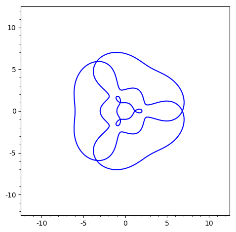
Figure 5: Intersection of $\mathbb{V}(F_{3})$ at $y_{3}=0$

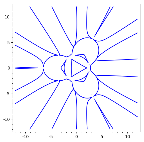
Figure 6: Intersection of $\mathbb{V}(F_{4})$ at $y_{3}=0$

The factors $F_{3}$ and $F_{4}$ yield surfaces of degree $28$ and $48$, respectively, which were not possible to be plotted nicely at once, but intersections with the plane $y_{3}=0$ are shown in Figs. 6 and 6, whereas intersections with $y_{2}=0$ are shown in Figs. 8 and 8.

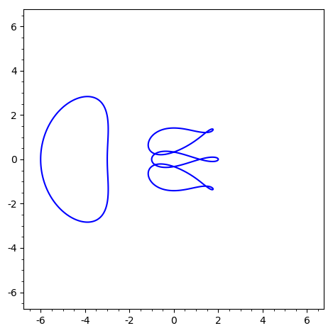
Figure 7: Intersection of $\mathbb{V}(F_{3})$ at $y_{2}=0$

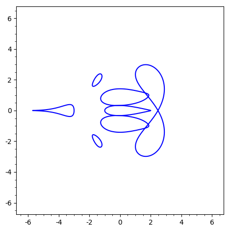
Figure 8: Intersection of $\mathbb{V}(F_{4})$ at $y_{2}=0$

Note that if one would differentiate the system $\cal W_{T}$, the factor $F_{4}$ does not appear in the determinant of the Jacobian of this system. Since $\cal W_{T}$ consists of constraint equations for the translational three-space, this approach yields poses where the manipulator can move infinitesimally in translational direction.

In the same way as it is done for the input singularities, it is possible to obtain a variety in joint space containing all output singularities via computing a Groebner basis of the system $\cal L$ that contains a polynomial depending on the input parameters only. Due to complexity reasons, symbolic computation was only possible for the simpler factor of the determinant of $\mathbf{J_{o}}$. This yields a polynomial of degree 12 in joint space, namely

$$144{{t_{1}}}^{4}{{t_{2}}}^{4}{{t_{3}}}^{4}+32{{t_{1}}}^{4}{{t_{2}}}^{4}{{t_{3}}}^{3}+32{{t_{1}}}^{4}{{t_{2}}}^{3}{{t_{3}}}^{4}+32{{t_{1}}}^{3}{{t_{2}}}^{4}{{t_{3}}}^{4}-272{{t_{1}}}^{4}{{t_{2}}}^{4}{{t_{3}}}^{2}-520{{t_{1}}}^{4}{{t_{2}}}^{3}{{t_{3}}}^{3}$$

$$-272{{t_{1}}}^{4}{{t_{2}}}^{2}{{t_{3}}}^{4}-520{{t_{1}}}^{3}{{t_{2}}}^{4}{{t_{3}}}^{3}-520{{t_{1}}}^{3}{{t_{2}}}^{3}{{t_{3}}}^{4}-272{{t_{1}}}^{2}{{t_{2}}}^{4}{{t_{3}}}^{4}-544{{t_{1}}}^{4}{{t_{2}}}^{4}{t_{3}}-1352{{t_{1}}}^{4}{{t_{2}}}^{3}{{t_{3}}}^{2}$$

$$-1352{{t_{1}}}^{4}{{t_{2}}}^{2}{{t_{3}}}^{3}-544{{t_{1}}}^{4}{t_{2}}{{t_{3}}}^{4}-1352{{t_{1}}}^{3}{{t_{2}}}^{4}{{t_{3}}}^{2}-1656{{t_{1}}}^{3}{{t_{2}}}^{3}{{t_{3}}}^{3}-1352{{t_{1}}}^{3}{{t_{2}}}^{2}{{t_{3}}}^{4}-1352{{t_{1}}}^{2}{{t_{2}}}^{4}{{t_{3}}}^{3}$$

$$-1352{{t_{1}}}^{2}{{t_{2}}}^{3}{{t_{3}}}^{4}-544{t_{1}}{{t_{2}}}^{4}{{t_{3}}}^{4}+16{{t_{1}}}^{4}{{t_{2}}}^{4}-1528{{t_{1}}}^{4}{{t_{2}}}^{3}{t_{3}}-3183{{t_{1}}}^{4}{{t_{2}}}^{2}{{t_{3}}}^{2}-1528{{t_{1}}}^{4}{t_{2}}{{t_{3}}}^{3}+16{{t_{1}}}^{4}{{t_{3}}}^{4}$$

$$-1528{{t_{1}}}^{3}{{t_{2}}}^{4}{t_{3}}-3182{{t_{1}}}^{3}{{t_{2}}}^{3}{{t_{3}}}^{2}-3182{{t_{1}}}^{3}{{t_{2}}}^{2}{{t_{3}}}^{3}-1528{{t_{1}}}^{3}{t_{2}}{{t_{3}}}^{4}-3183{{t_{1}}}^{2}{{t_{2}}}^{4}{{t_{3}}}^{2}-3182{{t_{1}}}^{2}{{t_{2}}}^{3}{{t_{3}}}^{3}$$

$$-3183{{t_{1}}}^{2}{{t_{2}}}^{2}{{t_{3}}}^{4}-1528{t_{1}}{{t_{2}}}^{4}{{t_{3}}}^{3}-1528{t_{1}}{{t_{2}}}^{3}{{t_{3}}}^{4}+16{{t_{2}}}^{4}{{t_{3}}}^{4}-448{{t_{1}}}^{4}{{t_{2}}}^{3}-2576{{t_{1}}}^{4}{{t_{2}}}^{2}{t_{3}}$$

$$-2576{{t_{1}}}^{4}{t_{2}}{{t_{3}}}^{2}-448{{t_{1}}}^{4}{{t_{3}}}^{3}-448{{t_{1}}}^{3}{{t_{2}}}^{4}-2520{{t_{1}}}^{3}{{t_{2}}}^{3}{t_{3}}-6880{{t_{1}}}^{3}{{t_{2}}}^{2}{{t_{3}}}^{2}-2520{{t_{1}}}^{3}{t_{2}}{{t_{3}}}^{3}$$

$$-448{{t_{1}}}^{3}{{t_{3}}}^{4}-2576{{t_{1}}}^{2}{{t_{2}}}^{4}{t_{3}}-6880{{t_{1}}}^{2}{{t_{2}}}^{3}{{t_{3}}}^{2}-6880{{t_{1}}}^{2}{{t_{2}}}^{2}{{t_{3}}}^{3}-2576{{t_{1}}}^{2}{t_{2}}{{t_{3}}}^{4}-2576{t_{1}}{{t_{2}}}^{4}{{t_{3}}}^{2}$$

$$-2520{t_{1}}{{t_{2}}}^{3}{{t_{3}}}^{3}-2576{t_{1}}{{t_{2}}}^{2}{{t_{3}}}^{4}-448{{t_{2}}}^{4}{{t_{3}}}^{3}-448{{t_{2}}}^{3}{{t_{3}}}^{4}-928{{t_{1}}}^{4}{{t_{2}}}^{2}-1480{{t_{1}}}^{4}{t_{2}}{t_{3}}-928{{t_{1}}}^{4}{{t_{3}}}^{2}$$

$$-1480{{t_{1}}}^{3}{{t_{2}}}^{3}-4562{{t_{1}}}^{3}{{t_{2}}}^{2}{t_{3}}-4562{{t_{1}}}^{3}{t_{2}}{{t_{3}}}^{2}-1480{{t_{1}}}^{3}{{t_{3}}}^{3}-928{{t_{1}}}^{2}{{t_{2}}}^{4}-4562{{t_{1}}}^{2}{{t_{2}}}^{3}{t_{3}}$$

$$-12486{{t_{1}}}^{2}{{t_{2}}}^{2}{{t_{3}}}^{2}-4562{{t_{1}}}^{2}{t_{2}}{{t_{3}}}^{3}-928{{t_{1}}}^{2}{{t_{3}}}^{4}-1480{t_{1}}{{t_{2}}}^{4}{t_{3}}-4562{t_{1}}{{t_{2}}}^{3}{{t_{3}}}^{2}-4562{t_{1}}{{t_{2}}}^{2}{{t_{3}}}^{3}$$

$$-1480{t_{1}}{t_{2}}{{t_{3}}}^{4}-928{{t_{2}}}^{4}{{t_{3}}}^{2}-1480{{t_{2}}}^{3}{{t_{3}}}^{3}-928{{t_{2}}}^{2}{{t_{3}}}^{4}-448{{t_{1}}}^{4}{t_{2}}-448{{t_{1}}}^{4}{t_{3}}-2576{{t_{1}}}^{3}{{t_{2}}}^{2}$$

$$-2520{{t_{1}}}^{3}{t_{2}}{t_{3}}-2576{{t_{1}}}^{3}{{t_{3}}}^{2}-2576{{t_{1}}}^{2}{{t_{2}}}^{3}-6880{{t_{1}}}^{2}{{t_{2}}}^{2}{t_{3}}-6880{{t_{1}}}^{2}{t_{2}}{{t_{3}}}^{2}-2576{{t_{1}}}^{2}{{t_{3}}}^{3}-448{t_{1}}{{t_{2}}}^{4}$$

$$-2520{t_{1}}{{t_{2}}}^{3}{t_{3}}-6880{t_{1}}{{t_{2}}}^{2}{{t_{3}}}^{2}-2520{t_{1}}{t_{2}}{{t_{3}}}^{3}-448{t_{1}}{{t_{3}}}^{4}-448{{t_{2}}}^{4}{t_{3}}-2576{{t_{2}}}^{3}{{t_{3}}}^{2}-2576{{t_{2}}}^{2}{{t_{3}}}^{3}$$

$$-448{t_{2}}{{t_{3}}}^{4}+16{{t_{1}}}^{4}-1528{{t_{1}}}^{3}{t_{2}}-1528{{t_{1}}}^{3}{t_{3}}-3183{{t_{1}}}^{2}{{t_{2}}}^{2}-3182{{t_{1}}}^{2}{t_{2}}{t_{3}}-3183{{t_{1}}}^{2}{{t_{3}}}^{2}-1528{t_{1}}{{t_{2}}}^{3}$$

$$-3182{t_{1}}{{t_{2}}}^{2}{t_{3}}-3182{t_{1}}{t_{2}}{{t_{3}}}^{2}-1528{t_{1}}{{t_{3}}}^{3}+16{{t_{2}}}^{4}-1528{{t_{2}}}^{3}{t_{3}}-3183{{t_{2}}}^{2}{{t_{3}}}^{2}-1528{t_{2}}{{t_{3}}}^{3}+16{{t_{3}}}^{4}$$

$$-544{{t_{1}}}^{3}-1352{{t_{1}}}^{2}{t_{2}}-1352{{t_{1}}}^{2}{t_{3}}-1352{t_{1}}{{t_{2}}}^{2}-1656{t_{1}}{t_{2}}{t_{3}}-1352{t_{1}}{{t_{3}}}^{2}-544{{t_{2}}}^{3}-1352{{t_{2}}}^{2}{t_{3}}$$

$$-1352{t_{2}}{{t_{3}}}^{2}-544{{t_{3}}}^{3}-272{{t_{1}}}^{2}-520{t_{1}}{t_{2}}-520{t_{1}}{t_{3}}-272{{t_{2}}}^{2}-520{t_{2}}{t_{3}}-272{{t_{3}}}^{2}+32{t_{1}}$$

$$+32{t_{2}}+32{t_{3}}+144$$

which defines a variety in joint space displayed in Fig. 10.

Now surfaces containing all input singularities of the translational operation mode of the 3-RUU PM have been determined in the space of Study parameters and in joint space as well as all surfaces containing all output singularities in the space of Study parameters. In joint space, the simpler of two varieties containing all output singularities has been determined. By intersecting these varieties one can easily find poses where the manipulator is simultaneously input and output singular. An admittedly impractical pose being both input and output singular is shown in Fig. 10.

Figure 9: Simpler component of output singularities in joint space

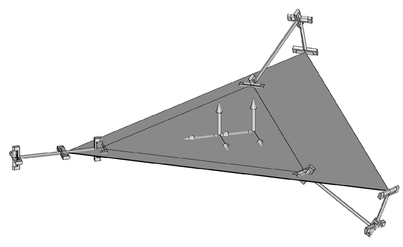
Figure 10: Simultaneous input and output singularity

4.3 Constraint Singularities

Constraint singularities are defined in [4]. Here they occur when the Jacobian $\mathbf{J}$ is rank defficient. This is the case if the determinants of all $8\times 8$ sub-matrices of $\mathbf{J}$ vanish. Since $\mathbf{J_{o}}$ is one of these sub-matrices, constraint singularities are in particular output singularities for this type of manipulator. Geometrically, the tangent space of the constraint variety gains dimensions in constraint singularities. Neglecting multiple coverings, these are the points, where different irreducible components intersect together with their self-intersections. Constraint singularities are not discussed in more detail since they are covered by the output singularity surface here, which need to be avoided in several kinematic tasks anyway, e.g. path planning.

Nonetheless it would be desirable to know if the 3-RUU PM can switch from the translational operation mode into another mode. To answer this question, one can check whether the components $O_{1}$ and $O_{3}$ have a non-empty intersection and thus a change between the respective operation modes is possible. Since there is no defining ideal for $O_{3}$ available it is difficult to compute this intersection. However, by a detailed inspection of the PM, a real curve $C(t)=[x_{0}(t),x_{1}(t),x_{2}(t),x_{3}(t),y_{0}(t),y_{1}(t),y_{2}(t),y_{3}(t)]$ can be constructed to be fully contained in the workspace. The geometry of the manipulator suggests, that rotations around the $y$-axis ($x_{0}(t)=1$, $x_{1}(t)=0$, $x_{3}(t)=0$) as well as translations parallel to the $xz$-plane ($y_{0}(t)=0$, $y_{1}(t)=0$) are possible. To further simplify the constraints, $y_{2}(t)$ is chosen to be zero. Setting $x_{2}(t)=t$, one can find $y_{3}(t)$ such that the curve lies on the workspace. For the design parameters

$$a_{1}=5,\leavevmode\nobreak\ a_{3}=4,\leavevmode\nobreak\ r_{0}=11,\leavevmode\nobreak\ r_{1}=7,$$ (11)

above’s procedure yields the real curve

$$C:[-1,1] \longrightarrow\mathbb{P}^{7}$$ (12)

$$t \longmapsto[1,0,t,0,0,0,0,h/4],$$

where

$$h\coloneqq 18t+\sqrt{25{t}^{2}+36}+\sqrt{{\frac{\left(-59{t}^{4}+212{t}^{2}+256\right)\sqrt{25{t}^{2}+36}-600{t}^{5}-864{t}^{3}}{\sqrt{25{t}^{2}+36}\left({t}^{2}+4\right)}}}.$$

It intersects the translational three-space $O_{1}$ only once, namely at the parameter value $t=0$. Even though this curve and its derivation is not of particular interest it does however provide a proof by example showing that the intersection $O_{1}\cap O_{3}$ is not empty. Thus the manipulator can indeed change between its operation modes. Note that because of symmetry, the same holds true for $\pm 120^{\circ}$ rotations about the $z$-axis of the motion induced by $C$. Fig. 11 shows two poses of the motion parameterized by $C$.

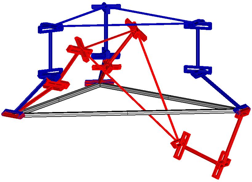
Figure 11: PM moving out of translational operation mode

4.4 Self-motions

A motion the manipulator can perform even though the actuated joints are locked, is called self-motion. Such a motion can be represented by a curve on the constraint variety with fixed input parameters. Tangents of this curve are independent of input parameters and are obviously contained in the tangent space of the constraint variety. Thus, the tangent space contains elements independent of the input parameters. Consequently, all points of such a curve are output singularities. Indeed, a self-motion was found in Section 4.2 for the specific design in Eq. (3). In the following, conditions on the design parameters of a 3-RUU PM will be derived, for which the manipulator has such a self-motion. Motivated by the results above, one is interested to calculate the intersection of $\mathbb{V}(F_{1})$ and $\mathbb{V}(F_{2})$. These varieties intersect in a circle contained in the plane $y_{3}=0$. The fact that the intersection is contained in this plane suggests to set the Study parameter $y_{3}$ to zero. Differentiating the general constraint equations for the translational operation mode $\mathcal{W_{T}}$ yields a $3\times 3$ Jacobian depending on $y_{1}$, $y_{2}$, $t_{1}$, $t_{2}$ and $t_{3}$. Similar to the procedure used in Section 4.2, the determinant of this matrix together with $\mathcal{W_{T}}$ yields a system of four equations. By successively eliminating the input parameters via computing resultants one obtains a polynomial expression, which has the factor

$${{a_{1}}}^{2}-{{a_{3}}}^{2}-(r_{0}-r_{1})^{2}+4\left({{y_{1}}}^{2}+{{y_{2}}}^{2}\right).$$

If one chooses design parameters such that ${a_{1}}^{2}-{a_{3}}^{2}-(r_{0}-r_{1})^{2}$ is negative, this factor defines a real circle. An easy computation shows, that every point on this circle can be reached with the fixed input parameters

$$t_{i}={\frac{-{a_{1}}\pm\sqrt{{{a_{1}}}^{2}-{{r_{0}}}^{2}+2{r_{0}}{r_{1}}-{{r_{1}}}^{2}}}{{r_{0}}-{r_{1}}}},$$

provided $r_{0}\neq r_{1}$ or $t_{i}=0$ in case $r_{0}=r_{1}$ for $i=1$, $2$, $3$ (compare to Eq. (10)). Fig. 12 shows two poses of this self-motion for the manipulator given by the design parameters in Eq. (11).

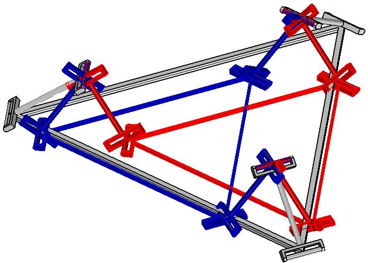
Figure 12: Two poses of the self-motion

5 Conclusion

A detailed singularity analysis of the translational operation mode of the 3-RUU parallel manipulator was given. Using a system of algebraic constraint equations, varieties containing input and output singularities could be determined in the Study space and in the joint space. Furthermore an input parameter free characterization of the overall workspace of the manipulator was found, to the best of the authors knowledge, for the first time. Numerical computations suggested that the workspace decomposes into three varieties of dimension three. Two of them are simple but unfortunately one of them seems to have impractically high degree. However, a curve on this component was found that intersects one of the simple components in a single point, thus transition between operation modes is possible. Finally, for this type of PM a self-motion was discovered. Future research should focus on the singularities of the general operation mode and on finding all poses of the end effector where the manipulator can switch between the operation modes.

Appendix

$$s_{1}: 18{{r_{0}}}^{2}{{t_{1}}}^{2}{{t_{2}}}^{2}{y_{3}}+18{{r_{0}}}^{2}{{t_{1}}}^{2}{{t_{3}}}^{2}{y_{3}}+18{{r_{0}}}^{2}{{t_{2}}}^{2}{{t_{3}}}^{2}{y_{3}}+18{{r_{1}}}^{2}{{t_{1}}}^{2}{{t_{2}}}^{2}{y_{3}}+18{{r_{1}}}^{2}{{t_{1}}}^{2}{{t_{3}}}^{2}{y_{3}}$$

$$+18{{r_{1}}}^{2}{{t_{2}}}^{2}{{t_{3}}}^{2}{y_{3}}+24{{a_{1}}}^{2}{t_{1}}{t_{2}}{y_{3}}+24{{a_{1}}}^{2}{t_{1}}{t_{3}}{y_{3}}+24{{a_{1}}}^{2}{t_{2}}{t_{3}}{y_{3}}-36{r_{0}}{r_{1}}{{t_{1}}}^{2}{y_{3}}-36{r_{0}}{r_{1}}{{t_{2}}}^{2}{y_{3}}$$

$$-36{r_{0}}{r_{1}}{{t_{3}}}^{2}{y_{3}}+24{a_{1}}{r_{0}}{t_{1}}{y_{3}}+24{a_{1}}{r_{0}}{t_{2}}{y_{3}}+24{a_{1}}{r_{0}}{t_{3}}{y_{3}}-24{a_{1}}{r_{1}}{t_{1}}{y_{3}}-24{a_{1}}{r_{1}}{t_{2}}{y_{3}}$$

$$-24{a_{1}}{r_{1}}{t_{3}}{y_{3}}+12{{a_{1}}}^{3}{t_{1}}{t_{3}}+12{{a_{1}}}^{3}{t_{2}}{t_{3}}-6{a_{1}}{r_{0}}{r_{1}}{{t_{3}}}^{2}-3{a_{1}}{{r_{0}}}^{2}{{t_{1}}}^{2}{{t_{3}}}^{2}-3{a_{1}}{{r_{0}}}^{2}{{t_{2}}}^{2}{{t_{3}}}^{2}$$

$$-3{a_{1}}{{r_{1}}}^{2}{{t_{1}}}^{2}{{t_{3}}}^{2}-3{a_{1}}{{r_{1}}}^{2}{{t_{2}}}^{2}{{t_{3}}}^{2}+12{a_{1}}{r_{0}}{{t_{1}}}^{2}{{t_{2}}}^{2}{y_{2}}\sqrt{3}-12{a_{1}}{r_{0}}{{t_{1}}}^{2}{{t_{3}}}^{2}{y_{2}}\sqrt{3}$$

$$-12{a_{1}}{r_{1}}{{t_{1}}}^{2}{{t_{2}}}^{2}{y_{2}}\sqrt{3}+12{a_{1}}{r_{1}}{{t_{1}}}^{2}{{t_{3}}}^{2}{y_{2}}\sqrt{3}-36{r_{0}}{r_{1}}{{t_{1}}}^{2}{{t_{2}}}^{2}{{t_{3}}}^{2}{y_{3}}+24{a_{1}}{r_{0}}{{t_{1}}}^{2}{{t_{2}}}^{2}{t_{3}}{y_{3}}$$

$$+24{a_{1}}{r_{0}}{{t_{1}}}^{2}{t_{2}}{{t_{3}}}^{2}{y_{3}}+24{a_{1}}{r_{0}}{t_{1}}{{t_{2}}}^{2}{{t_{3}}}^{2}{y_{3}}-24{a_{1}}{r_{1}}{{t_{1}}}^{2}{{t_{2}}}^{2}{t_{3}}{y_{3}}-24{a_{1}}{r_{1}}{{t_{1}}}^{2}{t_{2}}{{t_{3}}}^{2}{y_{3}}$$

$$-24{a_{1}}{r_{1}}{t_{1}}{{t_{2}}}^{2}{{t_{3}}}^{2}{y_{3}}+18{{r_{0}}}^{2}{y_{3}}+18{{r_{1}}}^{2}{y_{3}}+12{a_{1}}{r_{0}}{{t_{2}}}^{2}{y_{2}}\sqrt{3}-12{a_{1}}{r_{0}}{{t_{3}}}^{2}{y_{2}}\sqrt{3}$$

$$-12{a_{1}}{r_{1}}{{t_{2}}}^{2}{y_{2}}\sqrt{3}+12{a_{1}}{r_{1}}{{t_{3}}}^{2}{y_{2}}\sqrt{3}+8{{a_{1}}}^{2}{{t_{1}}}^{2}{t_{2}}{y_{2}}\sqrt{3}-8{{a_{1}}}^{2}{{t_{1}}}^{2}{t_{3}}{y_{2}}\sqrt{3}+16{{a_{1}}}^{2}\sqrt{3}{t_{1}}{{t_{2}}}^{2}{y_{2}}$$

$$-16{{a_{1}}}^{2}\sqrt{3}{t_{1}}{{t_{3}}}^{2}{y_{2}}+8{{a_{1}}}^{2}{t_{3}}{{t_{2}}}^{2}{y_{2}}\sqrt{3}+18{a_{1}}{r_{0}}{r_{1}}{{t_{1}}}^{2}{{t_{2}}}^{2}{{t_{3}}}^{2}+9{a_{1}}{{r_{1}}}^{2}+12{{a_{1}}}^{3}{t_{1}}{t_{2}}$$

$$+6{a_{1}}{r_{0}}{r_{1}}{{t_{1}}}^{2}{{t_{2}}}^{2}+6{a_{1}}{r_{0}}{r_{1}}{{t_{1}}}^{2}{{t_{3}}}^{2}-12{{a_{1}}}^{2}{r_{0}}{{t_{1}}}^{2}{{t_{2}}}^{2}{t_{3}}-12{{a_{1}}}^{2}{r_{0}}{{t_{1}}}^{2}{t_{2}}{{t_{3}}}^{2}-12{{a_{1}}}^{2}{r_{0}}{t_{1}}{{t_{2}}}^{2}{{t_{3}}}^{2}$$

$$+6{a_{1}}{r_{0}}{r_{1}}{{t_{2}}}^{2}{{t_{3}}}^{2}+9{a_{1}}{{r_{0}}}^{2}-12{{a_{1}}}^{2}{r_{1}}{t_{2}}-12{{a_{1}}}^{2}{r_{1}}{t_{1}}+12{{a_{1}}}^{2}{r_{1}}{{t_{1}}}^{2}{{t_{2}}}^{2}{t_{3}}+12{{a_{1}}}^{2}{r_{1}}{{t_{1}}}^{2}{t_{2}}{{t_{3}}}^{2}$$

$$+12{{a_{1}}}^{2}{r_{1}}{t_{1}}{{t_{2}}}^{2}{{t_{3}}}^{2}+18{{r_{0}}}^{2}{{t_{1}}}^{2}{{t_{2}}}^{2}{{t_{3}}}^{2}{y_{3}}+18{{r_{1}}}^{2}{{t_{1}}}^{2}{{t_{2}}}^{2}{{t_{3}}}^{2}{y_{3}}+24{{a_{1}}}^{2}{{t_{1}}}^{2}{t_{2}}{t_{3}}{y_{3}}+24{{a_{1}}}^{2}{t_{1}}{{t_{2}}}^{2}{t_{3}}{y_{3}}$$

$$+24{{a_{1}}}^{2}{t_{1}}{t_{2}}{{t_{3}}}^{2}{y_{3}}-36{r_{0}}{r_{1}}{{t_{1}}}^{2}{{t_{2}}}^{2}{y_{3}}-36{r_{0}}{r_{1}}{{t_{1}}}^{2}{{t_{3}}}^{2}{y_{3}}-36{r_{0}}{r_{1}}{{t_{2}}}^{2}{{t_{3}}}^{2}{y_{3}}+24{a_{1}}{r_{0}}{{t_{1}}}^{2}{t_{2}}{y_{3}}$$

$$+24{a_{1}}{r_{0}}{{t_{1}}}^{2}{t_{3}}{y_{3}}+24{a_{1}}{r_{0}}{t_{1}}{{t_{2}}}^{2}{y_{3}}+24{a_{1}}{r_{0}}{t_{1}}{{t_{3}}}^{2}{y_{3}}+24{a_{1}}{r_{0}}{{t_{2}}}^{2}{t_{3}}{y_{3}}+24{a_{1}}{r_{0}}{t_{2}}{{t_{3}}}^{2}{y_{3}}$$

$$-24{a_{1}}{r_{1}}{{t_{1}}}^{2}{t_{2}}{y_{3}}-24{a_{1}}{r_{1}}{{t_{1}}}^{2}{t_{3}}{y_{3}}-24{a_{1}}{r_{1}}{t_{1}}{{t_{2}}}^{2}{y_{3}}-24{a_{1}}{r_{1}}{t_{1}}{{t_{3}}}^{2}{y_{3}}-24{a_{1}}{r_{1}}{{t_{2}}}^{2}{t_{3}}{y_{3}}$$

$$-24{a_{1}}{r_{1}}{t_{2}}{{t_{3}}}^{2}{y_{3}}+18{{r_{0}}}^{2}{{t_{1}}}^{2}{y_{3}}+18{{r_{0}}}^{2}{{t_{2}}}^{2}{y_{3}}+18{{r_{0}}}^{2}{{t_{3}}}^{2}{y_{3}}+18{{r_{1}}}^{2}{{t_{1}}}^{2}{y_{3}}+18{{r_{1}}}^{2}{{t_{2}}}^{2}{y_{3}}$$

$$+18{{r_{1}}}^{2}{{t_{3}}}^{2}{y_{3}}-36{r_{0}}{r_{1}}{y_{3}}-12{a_{1}}{r_{1}}{{t_{1}}}^{2}{{t_{2}}}^{2}{y_{1}}-12{a_{1}}{r_{1}}{{t_{1}}}^{2}{{t_{3}}}^{2}{y_{1}}+24{a_{1}}{r_{1}}{{t_{2}}}^{2}{{t_{3}}}^{2}{y_{1}}$$

$$+12{a_{1}}{r_{0}}{{t_{1}}}^{2}{{t_{2}}}^{2}{y_{1}}+12{a_{1}}{r_{0}}{{t_{1}}}^{2}{{t_{3}}}^{2}{y_{1}}-24{a_{1}}{r_{0}}{{t_{2}}}^{2}{{t_{3}}}^{2}{y_{1}}+3{a_{1}}{{r_{0}}}^{2}{{t_{1}}}^{2}+3{a_{1}}{{r_{0}}}^{2}{{t_{2}}}^{2}+3{a_{1}}{{r_{0}}}^{2}{{t_{3}}}^{2}$$

$$+3{a_{1}}{{r_{1}}}^{2}{{t_{1}}}^{2}+3{a_{1}}{{r_{1}}}^{2}{{t_{2}}}^{2}+3{a_{1}}{{r_{1}}}^{2}{{t_{3}}}^{2}-9{a_{1}}{{r_{0}}}^{2}{{t_{1}}}^{2}{{t_{2}}}^{2}{{t_{3}}}^{2}-9{a_{1}}{{r_{1}}}^{2}{{t_{1}}}^{2}{{t_{2}}}^{2}{{t_{3}}}^{2}-18{a_{1}}{r_{0}}{r_{1}}$$

$$+12{{a_{1}}}^{2}{r_{0}}{t_{1}}+12{{a_{1}}}^{2}{r_{0}}{t_{2}}+12{{a_{1}}}^{2}{r_{0}}{t_{3}}-12{{a_{1}}}^{2}{r_{1}}{t_{3}}+24{{a_{1}}}^{2}{{t_{1}}}^{2}{t_{2}}{y_{1}}+24{{a_{1}}}^{2}{{t_{1}}}^{2}{t_{3}}{y_{1}}$$

$$-24{{a_{1}}}^{2}{{t_{2}}}^{2}{t_{3}}{y_{1}}-24{{a_{1}}}^{2}{t_{2}}{{t_{3}}}^{2}{y_{1}}+24{a_{1}}{r_{0}}{{t_{1}}}^{2}{y_{1}}-12{a_{1}}{r_{0}}{{t_{2}}}^{2}{y_{1}}-12{a_{1}}{r_{0}}{{t_{3}}}^{2}{y_{1}}-24{a_{1}}{r_{1}}{{t_{1}}}^{2}{y_{1}}$$

$$+12{a_{1}}{r_{1}}{{t_{2}}}^{2}{y_{1}}+12{a_{1}}{r_{1}}{{t_{3}}}^{2}{y_{1}}-8{{a_{1}}}^{2}{t_{2}}{{t_{3}}}^{2}{y_{2}}\sqrt{3}-3{a_{1}}{{r_{0}}}^{2}{{t_{1}}}^{2}{{t_{2}}}^{2}-3{a_{1}}{{r_{1}}}^{2}{{t_{1}}}^{2}{{t_{2}}}^{2}-6{a_{1}}{r_{0}}{r_{1}}{{t_{1}}}^{2}$$

$$-6{a_{1}}{r_{0}}{r_{1}}{{t_{2}}}^{2}-12{{a_{1}}}^{3}{{t_{1}}}^{2}{t_{2}}{t_{3}}-12{{a_{1}}}^{3}{t_{1}}{{t_{2}}}^{2}{t_{3}}-12{{a_{1}}}^{3}{t_{1}}{t_{2}}{{t_{3}}}^{2}$$

$$s_{2}: {a_{1}}{{t_{1}}}^{2}{{t_{2}}}^{2}{{y_{1}}}^{2}+{a_{1}}{{t_{1}}}^{2}{{t_{3}}}^{2}{{y_{1}}}^{2}-5{a_{1}}{{t_{2}}}^{2}{{t_{3}}}^{2}{{y_{1}}}^{2}-6{{r_{0}}}^{2}{{t_{1}}}^{2}{{t_{2}}}^{2}{y_{3}}-6{{r_{0}}}^{2}{{t_{1}}}^{2}{{t_{3}}}^{2}{y_{3}}-6{{r_{0}}}^{2}{{t_{2}}}^{2}{{t_{3}}}^{2}{y_{3}}$$

$$-6{{r_{1}}}^{2}{{t_{1}}}^{2}{{t_{2}}}^{2}{y_{3}}-6{{r_{1}}}^{2}{{t_{1}}}^{2}{{t_{3}}}^{2}{y_{3}}-6{{r_{1}}}^{2}{{t_{2}}}^{2}{{t_{3}}}^{2}{y_{3}}-8{{a_{1}}}^{2}{t_{1}}{t_{2}}{y_{3}}-8{{a_{1}}}^{2}{t_{1}}{t_{3}}{y_{3}}-8{{a_{1}}}^{2}{t_{2}}{t_{3}}{y_{3}}$$

$$+12{r_{0}}{r_{1}}{{t_{1}}}^{2}{y_{3}}+12{r_{0}}{r_{1}}{{t_{2}}}^{2}{y_{3}}+12{r_{0}}{r_{1}}{{t_{3}}}^{2}{y_{3}}-8{a_{1}}{r_{0}}{t_{1}}{y_{3}}-8{a_{1}}{r_{0}}{t_{2}}{y_{3}}-8{a_{1}}{r_{0}}{t_{3}}{y_{3}}$$

$$+8{a_{1}}{r_{1}}{t_{1}}{y_{3}}+8{a_{1}}{r_{1}}{t_{2}}{y_{3}}+8{a_{1}}{r_{1}}{t_{3}}{y_{3}}+6{{t_{1}}}^{2}{{t_{2}}}^{2}{{y_{1}}}^{2}{y_{3}}+6{{t_{1}}}^{2}{{t_{2}}}^{2}{{y_{2}}}^{2}{y_{3}}+6{{t_{1}}}^{2}{{t_{3}}}^{2}{{y_{1}}}^{2}{y_{3}}$$

$$+6{{t_{1}}}^{2}{{t_{3}}}^{2}{{y_{2}}}^{2}{y_{3}}+6{{t_{2}}}^{2}{{t_{3}}}^{2}{{y_{1}}}^{2}{y_{3}}+6{{t_{2}}}^{2}{{t_{3}}}^{2}{{y_{2}}}^{2}{y_{3}}+8{a_{1}}{t_{1}}{y_{1}}{y_{3}}-4{a_{1}}{t_{2}}{y_{1}}{y_{3}}-4{a_{1}}{t_{3}}{y_{1}}{y_{3}}$$

$$-4{{a_{1}}}^{3}{t_{1}}{t_{3}}-4{{a_{1}}}^{3}{t_{2}}{t_{3}}+2{a_{1}}{r_{0}}{r_{1}}{{t_{3}}}^{2}+{a_{1}}{{r_{0}}}^{2}{{t_{1}}}^{2}{{t_{3}}}^{2}+{a_{1}}{{r_{0}}}^{2}{{t_{2}}}^{2}{{t_{3}}}^{2}+{a_{1}}{{r_{1}}}^{2}{{t_{1}}}^{2}{{t_{3}}}^{2}+{a_{1}}{{r_{1}}}^{2}{{t_{2}}}^{2}{{t_{3}}}^{2}$$

$$+2{{a_{1}}}^{2}{{t_{1}}}^{2}{t_{3}}{{t_{2}}}^{2}{y_{2}}\sqrt{3}-2{{a_{1}}}^{2}{{t_{1}}}^{2}{t_{2}}{{t_{3}}}^{2}{y_{2}}\sqrt{3}-2{a_{1}}{r_{0}}{{t_{1}}}^{2}{{t_{2}}}^{2}{y_{2}}\sqrt{3}+2{a_{1}}{r_{0}}{{t_{1}}}^{2}{{t_{3}}}^{2}{y_{2}}\sqrt{3}$$

$$+2{a_{1}}{r_{1}}{{t_{1}}}^{2}{{t_{2}}}^{2}{y_{2}}\sqrt{3}-2{a_{1}}{r_{1}}{{t_{1}}}^{2}{{t_{3}}}^{2}{y_{2}}\sqrt{3}-4{a_{1}}{{t_{1}}}^{2}{{t_{2}}}^{2}{y_{1}}{y_{2}}\sqrt{3}+4{a_{1}}{{t_{1}}}^{2}{{t_{3}}}^{2}{y_{1}}{y_{2}}\sqrt{3}$$

$$+4{a_{1}}{{t_{1}}}^{2}\sqrt{3}{t_{2}}{y_{2}}{y_{3}}-4{a_{1}}{{t_{1}}}^{2}\sqrt{3}{t_{3}}{y_{2}}{y_{3}}-4{a_{1}}{{t_{2}}}^{2}\sqrt{3}{t_{3}}{y_{2}}{y_{3}}+4{a_{1}}\sqrt{3}{t_{2}}{{t_{3}}}^{2}{y_{2}}{y_{3}}+2{{a_{1}}}^{2}{t_{2}}{y_{2}}\sqrt{3}$$

$$-2{{a_{1}}}^{2}{t_{3}}{y_{2}}\sqrt{3}+12{r_{0}}{r_{1}}{{t_{1}}}^{2}{{t_{2}}}^{2}{{t_{3}}}^{2}{y_{3}}-8{a_{1}}{r_{0}}{{t_{1}}}^{2}{{t_{2}}}^{2}{t_{3}}{y_{3}}-8{a_{1}}{r_{0}}{{t_{1}}}^{2}{t_{2}}{{t_{3}}}^{2}{y_{3}}-8{a_{1}}{r_{0}}{t_{1}}{{t_{2}}}^{2}{{t_{3}}}^{2}{y_{3}}$$

$$+8{a_{1}}{r_{1}}{{t_{1}}}^{2}{{t_{2}}}^{2}{t_{3}}{y_{3}}+8{a_{1}}{r_{1}}{{t_{1}}}^{2}{t_{2}}{{t_{3}}}^{2}{y_{3}}+8{a_{1}}{r_{1}}{t_{1}}{{t_{2}}}^{2}{{t_{3}}}^{2}{y_{3}}-4{a_{1}}{{t_{1}}}^{2}{{t_{2}}}^{2}{t_{3}}{y_{1}}{y_{3}}-4{a_{1}}{{t_{1}}}^{2}{t_{2}}{{t_{3}}}^{2}{y_{1}}{y_{3}}$$

$$+8{a_{1}}{t_{1}}{{t_{2}}}^{2}{{t_{3}}}^{2}{y_{1}}{y_{3}}-4{a_{1}}{{t_{1}}}^{2}{{t_{2}}}^{2}\sqrt{3}{t_{3}}{y_{2}}{y_{3}}+4{a_{1}}{{t_{1}}}^{2}\sqrt{3}{t_{2}}{{t_{3}}}^{2}{y_{2}}{y_{3}}+3{a_{1}}{{y_{1}}}^{2}-6{{r_{0}}}^{2}{y_{3}}-6{{r_{1}}}^{2}{y_{3}}$$

$$+6{{y_{1}}}^{2}{y_{3}}+6{{y_{2}}}^{2}{y_{3}}-2{a_{1}}{r_{0}}{{t_{2}}}^{2}{y_{2}}\sqrt{3}+2{a_{1}}{r_{0}}{{t_{3}}}^{2}{y_{2}}\sqrt{3}+2{a_{1}}{r_{1}}{{t_{2}}}^{2}{y_{2}}\sqrt{3}-2{a_{1}}{r_{1}}{{t_{3}}}^{2}{y_{2}}\sqrt{3}$$

$$-4{a_{1}}{{t_{2}}}^{2}{y_{1}}{y_{2}}\sqrt{3}+4{a_{1}}{{t_{3}}}^{2}{y_{1}}{y_{2}}\sqrt{3}+4{a_{1}}\sqrt{3}{t_{2}}{y_{2}}{y_{3}}-4{a_{1}}\sqrt{3}{t_{3}}{y_{2}}{y_{3}}-2{{a_{1}}}^{2}{{t_{1}}}^{2}{t_{2}}{y_{2}}\sqrt{3}$$

$$+2{{a_{1}}}^{2}{{t_{1}}}^{2}{t_{3}}{y_{2}}\sqrt{3}-4{{a_{1}}}^{2}\sqrt{3}{t_{1}}{{t_{2}}}^{2}{y_{2}}+4{{a_{1}}}^{2}\sqrt{3}{t_{1}}{{t_{3}}}^{2}{y_{2}}-2{{a_{1}}}^{2}{t_{3}}{{t_{2}}}^{2}{y_{2}}\sqrt{3}-6{a_{1}}{r_{0}}{r_{1}}{{t_{1}}}^{2}{{t_{2}}}^{2}{{t_{3}}}^{2}$$

$$-3{a_{1}}{{r_{1}}}^{2}-4{{a_{1}}}^{3}{t_{1}}{t_{2}}-3{a_{1}}{{t_{1}}}^{2}{{t_{2}}}^{2}{{y_{2}}}^{2}-3{a_{1}}{{t_{1}}}^{2}{{t_{3}}}^{2}{{y_{2}}}^{2}+3{a_{1}}{{t_{2}}}^{2}{{t_{3}}}^{2}{{y_{2}}}^{2}+3{a_{1}}{{y_{2}}}^{2}$$

$$-3{a_{1}}{{t_{1}}}^{2}{{t_{2}}}^{2}{{t_{3}}}^{2}{{y_{1}}}^{2}+2{{a_{1}}}^{2}{{t_{1}}}^{2}{{t_{2}}}^{2}{t_{3}}{y_{1}}+2{{a_{1}}}^{2}{{t_{1}}}^{2}{t_{2}}{{t_{3}}}^{2}{y_{1}}-4{{a_{1}}}^{2}{t_{1}}{{t_{2}}}^{2}{{t_{3}}}^{2}{y_{1}}-2{a_{1}}{r_{0}}{r_{1}}{{t_{1}}}^{2}{{t_{2}}}^{2}$$

$$-2{a_{1}}{r_{0}}{r_{1}}{{t_{1}}}^{2}{{t_{3}}}^{2}+4{{a_{1}}}^{2}{r_{0}}{{t_{1}}}^{2}{{t_{2}}}^{2}{t_{3}}+4{{a_{1}}}^{2}{r_{0}}{{t_{1}}}^{2}{t_{2}}{{t_{3}}}^{2}+4{{a_{1}}}^{2}{r_{0}}{t_{1}}{{t_{2}}}^{2}{{t_{3}}}^{2}-3{a_{1}}{{t_{1}}}^{2}{{t_{2}}}^{2}{{t_{3}}}^{2}{{y_{2}}}^{2}$$

$$-2{a_{1}}{r_{0}}{r_{1}}{{t_{2}}}^{2}{{t_{3}}}^{2}-3{a_{1}}{{r_{0}}}^{2}+4{{a_{1}}}^{2}{r_{1}}{t_{2}}+4{{a_{1}}}^{2}{r_{1}}{t_{1}}-4{{a_{1}}}^{2}{r_{1}}{{t_{1}}}^{2}{{t_{2}}}^{2}{t_{3}}-4{{a_{1}}}^{2}{r_{1}}{{t_{1}}}^{2}{t_{2}}{{t_{3}}}^{2}$$

$$-4{{a_{1}}}^{2}{r_{1}}{t_{1}}{{t_{2}}}^{2}{{t_{3}}}^{2}-6{{r_{0}}}^{2}{{t_{1}}}^{2}{{t_{2}}}^{2}{{t_{3}}}^{2}{y_{3}}-6{{r_{1}}}^{2}{{t_{1}}}^{2}{{t_{2}}}^{2}{{t_{3}}}^{2}{y_{3}}-8{{a_{1}}}^{2}{{t_{1}}}^{2}{t_{2}}{t_{3}}{y_{3}}-8{{a_{1}}}^{2}{t_{1}}{{t_{2}}}^{2}{t_{3}}{y_{3}}$$

$$-8{{a_{1}}}^{2}{t_{1}}{t_{2}}{{t_{3}}}^{2}{y_{3}}+12{r_{0}}{r_{1}}{{t_{1}}}^{2}{{t_{2}}}^{2}{y_{3}}+12{r_{0}}{r_{1}}{{t_{1}}}^{2}{{t_{3}}}^{2}{y_{3}}+12{r_{0}}{r_{1}}{{t_{2}}}^{2}{{t_{3}}}^{2}{y_{3}}-8{a_{1}}{r_{0}}{{t_{1}}}^{2}{t_{2}}{y_{3}}$$

$$-8{a_{1}}{r_{0}}{{t_{1}}}^{2}{t_{3}}{y_{3}}-8{a_{1}}{r_{0}}{t_{1}}{{t_{2}}}^{2}{y_{3}}-8{a_{1}}{r_{0}}{t_{1}}{{t_{3}}}^{2}{y_{3}}-8{a_{1}}{r_{0}}{{t_{2}}}^{2}{t_{3}}{y_{3}}-8{a_{1}}{r_{0}}{t_{2}}{{t_{3}}}^{2}{y_{3}}+8{a_{1}}{r_{1}}{{t_{1}}}^{2}{t_{2}}{y_{3}}$$

$$+8{a_{1}}{r_{1}}{{t_{1}}}^{2}{t_{3}}{y_{3}}+8{a_{1}}{r_{1}}{t_{1}}{{t_{2}}}^{2}{y_{3}}+8{a_{1}}{r_{1}}{t_{1}}{{t_{3}}}^{2}{y_{3}}+8{a_{1}}{r_{1}}{{t_{2}}}^{2}{t_{3}}{y_{3}}+8{a_{1}}{r_{1}}{t_{2}}{{t_{3}}}^{2}{y_{3}}$$

$$+6{{t_{1}}}^{2}{{t_{2}}}^{2}{{t_{3}}}^{2}{{y_{1}}}^{2}{y_{3}}+6{{t_{1}}}^{2}{{t_{2}}}^{2}{{t_{3}}}^{2}{{y_{2}}}^{2}{y_{3}}-4{a_{1}}{{t_{1}}}^{2}{t_{2}}{y_{1}}{y_{3}}-4{a_{1}}{{t_{1}}}^{2}{t_{3}}{y_{1}}{y_{3}}+8{a_{1}}{t_{1}}{{t_{2}}}^{2}{y_{1}}{y_{3}}$$

$$+8{a_{1}}{t_{1}}{{t_{3}}}^{2}{y_{1}}{y_{3}}-4{a_{1}}{{t_{2}}}^{2}{t_{3}}{y_{1}}{y_{3}}-4{a_{1}}{t_{2}}{{t_{3}}}^{2}{y_{1}}{y_{3}}+6{{t_{1}}}^{2}{{y_{1}}}^{2}{y_{3}}+6{{t_{1}}}^{2}{{y_{2}}}^{2}{y_{3}}+6{{t_{2}}}^{2}{{y_{1}}}^{2}{y_{3}}$$

$$+6{{t_{2}}}^{2}{{y_{2}}}^{2}{y_{3}}+6{{t_{3}}}^{2}{{y_{1}}}^{2}{y_{3}}+6{{t_{3}}}^{2}{{y_{2}}}^{2}{y_{3}}-6{{r_{0}}}^{2}{{t_{1}}}^{2}{y_{3}}-6{{r_{0}}}^{2}{{t_{2}}}^{2}{y_{3}}-6{{r_{0}}}^{2}{{t_{3}}}^{2}{y_{3}}-6{{r_{1}}}^{2}{{t_{1}}}^{2}{y_{3}}$$

$$-6{{r_{1}}}^{2}{{t_{2}}}^{2}{y_{3}}-6{{r_{1}}}^{2}{{t_{3}}}^{2}{y_{3}}+12{r_{0}}{r_{1}}{y_{3}}+2{a_{1}}{r_{1}}{{t_{1}}}^{2}{{t_{2}}}^{2}{y_{1}}+2{a_{1}}{r_{1}}{{t_{1}}}^{2}{{t_{3}}}^{2}{y_{1}}-4{a_{1}}{r_{1}}{{t_{2}}}^{2}{{t_{3}}}^{2}{y_{1}}$$

$$-2{a_{1}}{r_{0}}{{t_{1}}}^{2}{{t_{2}}}^{2}{y_{1}}-2{a_{1}}{r_{0}}{{t_{1}}}^{2}{{t_{3}}}^{2}{y_{1}}+4{a_{1}}{r_{0}}{{t_{2}}}^{2}{{t_{3}}}^{2}{y_{1}}+4{{a_{1}}}^{2}{t_{1}}{y_{1}}-2{{a_{1}}}^{2}{t_{2}}{y_{1}}-2{{a_{1}}}^{2}{t_{3}}{y_{1}}$$

$$+5{a_{1}}{{t_{1}}}^{2}{{y_{1}}}^{2}-{a_{1}}{{t_{2}}}^{2}{{y_{1}}}^{2}-{a_{1}}{{t_{3}}}^{2}{{y_{1}}}^{2}-{a_{1}}{{r_{0}}}^{2}{{t_{1}}}^{2}-{a_{1}}{{r_{0}}}^{2}{{t_{2}}}^{2}-{a_{1}}{{r_{0}}}^{2}{{t_{3}}}^{2}-{a_{1}}{{r_{1}}}^{2}{{t_{1}}}^{2}-{a_{1}}{{r_{1}}}^{2}{{t_{2}}}^{2}$$

$$-{a_{1}}{{r_{1}}}^{2}{{t_{3}}}^{2}+3{a_{1}}{{r_{0}}}^{2}{{t_{1}}}^{2}{{t_{2}}}^{2}{{t_{3}}}^{2}+3{a_{1}}{{r_{1}}}^{2}{{t_{1}}}^{2}{{t_{2}}}^{2}{{t_{3}}}^{2}+6{a_{1}}{r_{0}}{r_{1}}-4{{a_{1}}}^{2}{r_{0}}{t_{1}}-4{{a_{1}}}^{2}{r_{0}}{t_{2}}-4{{a_{1}}}^{2}{r_{0}}{t_{3}}$$

$$+4{{a_{1}}}^{2}{r_{1}}{t_{3}}-6{{a_{1}}}^{2}{{t_{1}}}^{2}{t_{2}}{y_{1}}-6{{a_{1}}}^{2}{{t_{1}}}^{2}{t_{3}}{y_{1}}+6{{a_{1}}}^{2}{{t_{2}}}^{2}{t_{3}}{y_{1}}+6{{a_{1}}}^{2}{t_{2}}{{t_{3}}}^{2}{y_{1}}-4{a_{1}}{r_{0}}{{t_{1}}}^{2}{y_{1}}$$

$$+2{a_{1}}{r_{0}}{{t_{2}}}^{2}{y_{1}}+2{a_{1}}{r_{0}}{{t_{3}}}^{2}{y_{1}}+4{a_{1}}{r_{1}}{{t_{1}}}^{2}{y_{1}}-2{a_{1}}{r_{1}}{{t_{2}}}^{2}{y_{1}}-2{a_{1}}{r_{1}}{{t_{3}}}^{2}{y_{1}}+2{{a_{1}}}^{2}{t_{2}}{{t_{3}}}^{2}{y_{2}}\sqrt{3}$$

$$+{a_{1}}{{r_{0}}}^{2}{{t_{1}}}^{2}{{t_{2}}}^{2}+{a_{1}}{{r_{1}}}^{2}{{t_{1}}}^{2}{{t_{2}}}^{2}+2{a_{1}}{r_{0}}{r_{1}}{{t_{1}}}^{2}+2{a_{1}}{r_{0}}{r_{1}}{{t_{2}}}^{2}+4{{a_{1}}}^{3}{{t_{1}}}^{2}{t_{2}}{t_{3}}+4{{a_{1}}}^{3}{t_{1}}{{t_{2}}}^{2}{t_{3}}$$

$$+4{{a_{1}}}^{3}{t_{1}}{t_{2}}{{t_{3}}}^{2}-3{a_{1}}{{t_{1}}}^{2}{{y_{2}}}^{2}+3{a_{1}}{{t_{2}}}^{2}{{y_{2}}}^{2}+3{a_{1}}{{t_{3}}}^{2}{{y_{2}}}^{2}.$$

References

- ATMC+ [12] S. Amine, M. Tale Masouleh, S. Caro, P. Wenger, and C. Gosselin. Singularity Conditions of 3T1R Parallel Manipulators With Identical Limb Structures. Journal of Mechanisms and Robotics, 4(1):1851 – 1863, 2012.
- Bat [13] D. J. Bates, J. D. Hauenstein, A. J. Sommese, and C. W. Wampler Numerically solving polynomial systems with Bertini, volume 25 of Software, Environments, and Tools. Society for Industrial and Applied Mathematics (SIAM), Philadelphia, PA, 2013.
- BTT [10] J. Borràs, F. Thomas, and C. Torras. Singularity-Invariant Leg Rearrangements in Stewart–Gough Platforms. In Jadran Lenarcic and Michael M. Stanisic, editors, Advances in Robot Kinematics: Motion in Man and Machine, pages 421–428, Dordrecht, 2010. Springer Netherlands.
- BZ [01] I. A. Bonev and D. Zlatanov. The Mystery of the Singular SNU Translational Parallel Robot, 06 2001.
- C. [90] C. Gosselin and J. Angeles. Singularity analysis of closed-loop kinematic chains. IEEE Transactions on Robotics and Automation, 6(3):281–290, Jun 1990.
- Den [55] J. Denavit, and R. S. Hartenberg A kinematic notation for lower-pair mechanisms based on matrices. Trans. ASME E, Journal of Applied Mechanics, 22:215–221, June 1955.
- DM [00] B. Dasgupta and T. S. Mruthyunjaya. The Stewart platform manipulator: a review. Mechanism and Machine Theory, 35(1):15 – 40, 2000.
- Geo [10] G. Nawratil. Stewart Gough platforms with linear singularity surface. In 19th International Workshop on Robotics in Alpe-Adria-Danube Region (RAAD 2010), pages 231–235, June 2010.
- HPSB [07] M. L. Husty, M. Pfurner, H.-P. Schröcker, and K. Brunnthaler. Algebraic Methods in Mechanism Analysis and Synthesis. Robotica, 25:661 – 675, 2007.
- Naw [10] G. Nawratil. Stewart Gough platforms with non-cubic singularity surface. Mechanism and Machine Theory, 45(12):1851 – 1863, 2010.
- Sch [14] J. Schadlbauer, D. R. Walter, and M. L. Husty The 3-RPS parallel manipulator from an algebraic viewpoint. Mechanism and Machine Theory, 75(Complete):161–176, 2014.
- SNC+ [18] T. Stigger, A. Nayak, S. Caro, P. Wenger, M. Pfurner, and M. L. Husty. Algebraic Analysis of a 3-RUU Parallel Manipulator. In J. Lenarcic and V. Parenti-Castelli, editors, Advances in Robot Kinematics 2018, volume 8 of Springer Proceedings in Advanced Robotics, pages 141–149, Bologna, Italy, 07 2018. Springer Cham.
- Sti [19] T. Stigger, M. Pfurner, and M. Husty. Workspace and Singularity Analysis of a 3-RUU Parallel Manipulator. In Corves, Burkhard and Wenger, Philippe and Hüsing, Mathias, editor, EuCoMeS 2018, pages 325–332, Cham, 2019. Springer International Publishing.