Functionals of fractional Brownian motion and the three arcsine laws

Abstract

Fractional Brownian motion is a non-Markovian Gaussian process indexed by the Hurst exponent $H\in[0,1]$, generalizing standard Brownian motion to account for anomalous diffusion. Functionals of this process are important for practical applications as a standard reference point for non-equilibrium dynamics. We describe a perturbation expansion allowing us to evaluate many non-trivial observables analytically: We generalize the celebrated three arcsine-laws of standard Brownian motion. The functionals are: (i) the fraction of time the process remains positive, (ii) the time when the process last visits the origin, and (iii) the time when it achieves its maximum (or minimum). We derive expressions for the probability of these three functionals as an expansion in $\varepsilon=H-\tfrac{1}{2}$, up to second order. We find that the three probabilities are different, except for $H=\tfrac{1}{2}$ where they coincide. Our results are confirmed to high precision by numerical simulations.

I Introduction

I.1 Fractional Brownian motion

In the theory of stochastic processes fractional Brownian motion (fBm) plays as important a role as standard Brownian motion [1, 2, 3, 4]. It was introduced [5, 6] to incorporate anomalous diffusive transport [7], which is abundant in nature, but not describable by standard Brownian motion. FBm has several key mathematical structures to qualify it as the most fundamental stochastic process for anomalous diffusion: translation invariance in both time and space (stationarity), invariance under rescaling, and Gaussianity [8]. The current mathematical formulation of fBm was given by Mandelbrot and Van Ness [6] to describe correlated time-series in natural processes. It is defined as a Gaussian stochastic process $X_{t}$ with $X_{0}=0$, mean $\left<X_{t}\right>=0$ and covariance

$$\langle X_{t}X_{s}\rangle=t^{2H}+s^{2H}-|t-s|^{2H}\ .$$ (1)

The parameter $H\in(0,1)$ is the Hurst exponent. An example is given in Fig. 1. Standard Brownian motion corresponds to $H=\tfrac{1}{2}$ where the covariance reduces to $\langle X_{t}X_{s}\rangle=2\min(s,t)$.

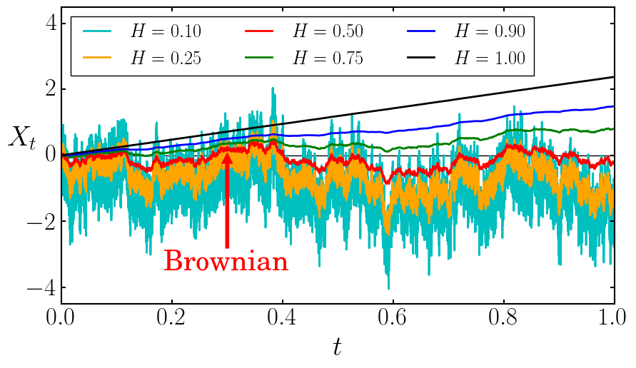
Figure 1: (color online) Sample trajectories of an fBm corresponding to different Hurst exponent ($H$). Anti-correlation of increments for $H<\frac{1}{2}$ can be seen from larger fluctuations of the trajectories. In comparison, smoother trajectories for $H>\frac{1}{2}$ reflect positive correlations, which become a straight line for $H\to 1$.

FBm is important as it successfully models a variety of natural processes [1, 2]: A tagged particle in single-file diffusion ($H\,{=}\,0.25$) [9, 10, 11, 12, 13], the integrated current in diffusive transport ($H\,{=}\,0.25$) [14], polymer translocation through a narrow pore ($H\,{\simeq}\,0.4$) [15, 16, 17], anomalous diffusion [18], values of the log return of a stock ($H\,{\simeq}\,0.6\;{\rm to}\;0.8$) [19, 20, 21, 22], hydrology ($H\,{\simeq}\,0.72\;{\rm to}\;0.87$) [23, 24], a tagged monomer in a polymer chain ($H\,{=}\,0.25$) [25], solar flare activity ($H\,{\simeq}\,0.57\;{\rm to}\;0.86$) [26], the price of electricity in a liberated market ($H\,{\simeq}\,0.41$) [27], telecommunication networks ($H\,{\simeq}\,0.78\;{\rm to}\;0.86$) [28], telomeres inside the nucleus of human cells ($H\,{\simeq}\,0.18\;{\rm to}\;0.35$) [29], sub-diffusion of lipid granules in yeast cells [30], and diffusion inside crowded fluids ($H\,{\simeq}\,0.4$) [31], are few such examples. Due to the simplicity of its definition, fBm has a fundamental importance, as well as a multitude of potential applications. The pressing questions are how the celebrated properties of standard Brownian motion generalize for fBm, and how can one analyze them? In this paper we aim to address some of these questions.

The anomalous diffusion in fBm comes from the long-range correlations in time, which makes the process non-Markovian, i.e. its increments are not independent, unless $H=\tfrac{1}{2}$; this can be seen from the correlation of increments,

$$\langle\partial_{t}X_{t}\,\partial_{s}X_{s}\rangle=2H(2H-1)|s-t|^{2(H-1)}\ .$$ (2)

The positivity of correlations for $H>\tfrac{1}{2}$ means that the process is correlated and the paths appear to be more regular than for standard Brownian motion. The converse holds for $H<\tfrac{1}{2}$, where increments are anti-correlated, making the process rough on short scales. This can be seen in Fig. 1 for the sample trajectory of a fBm generated in our computer simulation, using the same random numbers for the Fourier modes, which renders the resulting curves comparable.

The non-Markovian dynamics makes a theoretical analysis of fBm difficult. Until now, few exact results are available in the literature [32, 33, 34]. In this paper, we describe a systematic theoretical approach to fBm, by constructing a perturbation theory in

$$\varepsilon=H-\frac{1}{2}$$ (3)

around the Markovian dynamics. We describe this approach with a focus on observables that are functionals of the fBm trajectory $X_{t}$, and thereby depend on the entire history of the process. The fraction of time $X_{t}$ remains positive, the area under $X_{t}$, the position of the last maximum, or the time where $X_{t}$ reaches its maximum are examples of such functionals.

Functionals of stochastic processes are a topic of general interest [35, 36]. Beside their relevance in addressing practical problems, they appear in path-ensemble generalizations of traditional statistical mechanics [37, 38]. Beyond equilibrium statistical mechanics, the dynamics plays a crucial role in the statistical theory of non-equilibrium systems. Observables that are functionals of a stochastic trajectory, e.g. entropy production, empirical work, integrated current, or activity, are relevant dynamical observables for a thermodynamic description of non-equilibrium systems [39].

The statistics of functionals is non-trivial already for Markovian processes, and is much harder for non-Markovian ones like fBm. In our work, we overcome the inherent difficulty of the non-Markovian dynamics of fBm by using a perturbation expansion around standard Brownian motion ($H=\tfrac{1}{2}$), which is a Markovian process. This allows us to use many tricks available for Brownian motion, such as the method of images.

I.2 The three arcsine laws

We illustrate this approach by considering a generalization of a famous result for standard Brownian motion: the three arcsine-laws [40, 41, 42, 43]. This result is about the following three functionals of a Brownian motion $B_{t}$ starting from the origin $B_{0}=0$, and evolving during time $T$ (see Fig. 2):

1. the total duration $t_{\rm pos}$ when the process is positive,

2. the last time $t_{\rm last}$ the process visits the origin, and

3. the time $t_{\rm max}$ it achieves its maximum (or minimum).

Remarkably, all three functionals have the same probability distribution as a function of $\vartheta:=t/T$, given by [40, 41, 42, 43]

$$p(\vartheta)=\frac{1}{{\pi\sqrt{\vartheta(1-\vartheta)}}}\ .$$ (4)

As the cumulative distribution contains an arcsine function, these laws are commonly referred to as the first, second, and third arcsine-law. These laws apply quite generally to Markov processes, i.e. processes where the increments are uncorrelated [41]. Their counter-intuitive form with a divergence at $\vartheta=0$ and $\vartheta=1$ has sparked a lot of interest, and they are considered among the most important results for stochastic processes. Recent studies led to many extensions, in constrained Brownian motion [44, 45, 46], for general stochastic processes [47, 48, 49, 50, 51, 52], and even in higher dimensions [53, 54, 55]. The laws are realized in a plethora of real-world examples, from finance [56, 57] to competitive team sports [58].

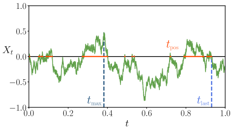
Figure 2: (color online) The three observables $t_{\rm pos}$, $t_{\rm last}$, and $t_{\rm max}$ for a stochastic process starting at the origin. For the standard Brownian motion, all three have the same cumulative probability distribution expressed in terms of arcsine function [40, 41, 42, 43].

Using our perturbative approach, we show how the three arcsine-laws generalize for fBm. Our results show that unlike for standard Brownian motion, all three functionals have different probability distributions, which coincide only when $\varepsilon=0$, i.e. for Brownian motion. As for two of the laws the difference is first seen at second order in $\varepsilon$, we have to develop the technology beyond what was done at leading order [59, 60, 61, 62, 63, 64, 65, 66]. Using our perturbation results up to second order, and a scaling ansatz, we propose expressions for all three probability densities. These expressions agree well with our numerical results, even for large values of $\varepsilon$, i.e. including the full range of Hurst exponents reported in the literature cited above [9, 10, 11, 12, 13, 14, 15, 16, 17, 18, 19, 20, 21, 22, 23, 24, 25, 26, 27, 28, 29, 30]. A short account of our main results was reported in [67].

This article is organized in the following order: In Sec. II we discuss basics of an fBm and introduce the perturbation expansion of the action. As a consistency check we derive the free propagator for an fBm in Sec. III, which is checked against the exact result. In the rest of the sections we discuss the three functionals for the arcsine-law. In Sec. IV, we summarize our main analytical results for the generalization of the arcsine laws for an fBm, and compare them with our numerical simulations. How these results are derived is first sketched in Sec. V, and thoroughly discussed in later sections. Many algebraic details and a description of our numerical algorithm are given in the appendices.

II Perturbation theory

II.1 The action to second order in $\varepsilon$

Our analysis is based on a perturbation expansion of the action for an fBm trajectory around standard Brownian motion ($H=\frac{1}{2}$). This expansion was discussed and used earlier in [59, 60, 62, 61, 63, 64, 65, 67, 66] at linear order. Here, we give additional details at second order, which is essential to show the difference between the generalizations of the three arcsine-laws.

An ensemble of trajectories for fBm in a time window $[0,T]$ is characterized by the Gaussian action

$$S[X_{t}]=\frac{1}{2}\int_{0}^{T}dt_{1}\int_{0}^{T}dt_{2}X_{t_{1}}G(t_{1},t_{2})X_{t_{2}}$$ (5)

with covariance $G^{-1}(t_{1},t_{2})=\langle X_{t_{1}}X_{t_{2}}\rangle$ as given in Eq. (1). The probability of a trajectory, up to a normalization, is given by

$$P[X_{t}]\sim e^{-S[X_{t}]}.$$ (6)

For $H=\frac{1}{2}$ one recovers the Feynman-Kac formula [68] for standard Brownian motion.

Writing $H=\frac{1}{2}+\varepsilon$ and expanding Eq. (5) in powers of $\varepsilon$ we obtain (a derivation is in App. A)

$$S=\frac{1}{D}\left[S_{0}-\frac{\varepsilon}{2}S_{1}+\varepsilon^{2}S_{2}+\cdots\right],$$ (7)

where

$$S_{0}= \frac{1}{4}\int_{0}^{T}dt\;\dot{x}(t)^{2},$$ (8a)

$$S_{1}= \int_{0}^{T}dr_{1}\int_{r_{1}+\omega}^{T}dr_{2}\;\frac{\dot{x}(r_{1})\dot{x}(r_{2})}{r_{2}-r_{1}},$$ (8b)

$$S_{2}= \frac{1}{2}\int_{0}^{T}dr_{1}\int_{r_{1}+\omega}^{T}dr_{2}\;\dot{x}(r_{1})\dot{x}(r_{2})\times$$ (8c)

$$\bigg{[}\int_{0}^{r_{1}-\omega}\!\!\!\!\!\!\frac{ds}{(r_{1}-s)(r_{2}-s)}+\int_{r_{2}+\omega}^{T}\frac{ds}{(s-r_{1})(s-r_{2})}\bigg{]}.~{}~{}~{}~{}~{}~{}$$

The pre-factor, the diffusion constant, reads

$$D\equiv D(\varepsilon,\omega)=e^{\varepsilon\,2(1+\ln\omega)-\varepsilon^{2}\,2(1-\frac{\pi^{2}}{6})+\mathcal{O}(\varepsilon^{3})}.$$ (9)

The small-time (ultraviolet) cutoff $\omega>0$ is introduced to regularize the integrals in the action. Our final results are in the limit of $\omega\rightarrow 0$, and independent of $\omega$. The second-order term in the exponential in Eq. (9) is independent of $\omega$, since from dimensional arguments $D\sim\omega^{\varepsilon}$,

• To keep our formulas simple, we explicitly write the ultraviolet cutoff in Eqs. (8b)-(8c) only for integrals which would otherwise diverge.

II.2 Integral representation of the action, and normal-ordered form of the weight

For our explicit calculations we use an alternative representation of Eqs. (8b) and (8c):

$$S_{1}=\int_{0}^{\Lambda}dy\int_{0}^{T}dr_{1}\int_{r_{1}}^{T}dr_{2}\,\dot{x}(r_{1})\dot{x}(r_{2})e^{y(r_{1}-r_{2})},$$ (10a)

and

$$S_{2}=\frac{1}{2} \int_{0}^{\Lambda}dy_{1}\int_{0}^{\Lambda}dy_{2}\int_{0}^{T}dr_{1}\int_{r_{1}}^{T}dr_{2}\,\dot{x}(r_{1})\dot{x}(r_{2})\times$$

$$\left[\int_{0}^{r_{1}}ds\;e^{-y_{1}(r_{1}-s)-y_{2}(r_{2}-s)}\;+\right.$$ (10b)

$$\left.\qquad\qquad\int_{r_{2}}^{T}ds\;e^{-y_{1}(s-r_{1})-y_{2}(s-r_{2})}\right],\qquad$$ (10c)

where the ultraviolet cutoff $$\omega \Lambda y \omega \Lambda\to\infty$$ in time is replaced by an upper limit for the variables. A vanishing is equivalent to , which is always taken in the final results.

Their relation can be inferred as follows: for small $\omega$

$$\int_{\omega}^{\infty}\frac{dt}{t}e^{-st}\simeq-\ln(s\,\omega)-\gamma_{\rm E}+\mathcal{O}(\omega),$$ (11)

where $\gamma_{\rm E}=0.57721\dots$ is the Euler constant. On the other hand, the integral representation for large $\Lambda$ reads

$$\int_{0}^{\Lambda}dy\int_{0}^{\infty}dt\;e^{-ts-ty}\simeq\ln\left(\frac{\Lambda}{s}\right)+\mathcal{O}(\Lambda^{-1}).$$ (12)

Demanding that they agree, we get

$$\Lambda=\frac{1}{\omega}e^{-\gamma_{\rm E}}.$$ (13)

In Sec. III we further check Eq. (13) by constructing the free diffusion propagator for fBm. In terms of $\Lambda$, Eq. (9) reads

$$D=e^{\varepsilon\;2(1-\ln\Lambda-\gamma_{\rm E})-\varepsilon^{2}\,2(1-\frac{\pi^{2}}{6})+\mathcal{O}(\varepsilon^{3})}.$$ (14)

• Keeping in mind the ultraviolet cutoff $\omega$ present in Eqs. (8b)–(8c), integrals arising from Eq. (10) are interpreted such that

  $$\int_{r_{1}}^{T}dr_{2}\;\delta(r_{2}-r_{1}):=\lim_{\omega\to 0}\int_{r_{1}+\omega}^{T}dr_{2}\;\delta(r_{2}-r_{1})=0.$$ (15)

  This convention for the expression of the action is used throughout our analysis.

A subtle point is that at second order for the probability in Eq. (6) one encounters terms of order $S_{1}^{2}$ in which one contracts two of the $\dot{x}$ (contracting all four gives a constant entering into the normalization of the probability, thus ignored),

$$\frac{S_{1}^{2}}{8} = \frac{1}{8}\int_{0}^{T}dr_{1}\int_{r_{1}+\omega}^{T}dr_{2}\;\frac{\dot{x}(r_{1})\dot{x}(r_{2})}{r_{2}-r_{1}}\times$$

$$\qquad\int_{0}^{T}dr_{3}\int_{r_{3}+\omega}^{T}dr_{4}\;\frac{\dot{x}(r_{3})\dot{x}(r_{4})}{r_{4}-r_{3}}$$

$$\longrightarrow\begin{cases}\frac{1}{4}\int_{r_{1}<r_{2},r_{4}}\;\frac{\dot{x}(r_{2})}{r_{2}-r_{1}}\frac{\dot{x}(r_{4})}{r_{4}-r_{1}}\\[10.0pt] \frac{1}{4}\int_{r_{3}<r_{1}<r_{2}}\frac{\dot{x}(r_{2})}{r_{2}-r_{1}}\frac{\dot{x}(r_{3})}{r_{1}-r_{3}}\\[10.0pt] \frac{1}{4}\int_{r_{1}<r_{2}<r_{4}}\;\frac{\dot{x}(r_{1})}{r_{2}-r_{1}}\frac{\dot{x}(r_{4})}{r_{4}-r_{2}}\\[10.0pt] \frac{1}{4}\int_{r_{1},r_{3}<r_{2}}\frac{\dot{x}(r_{1})}{r_{2}-r_{1}}\frac{\dot{x}(r_{3})}{r_{2}-r_{3}}.\end{cases}$$

The cutoffs in the integrations are implicit and the right arrow indicates contraction of a pair of $\dot{x}$. The four terms come, in the given order, from the contraction of $\dot{x}(r_{1})\dot{x}(r_{3})$, $\dot{x}(r_{1})\dot{x}(r_{4})$, $\dot{x}(r_{2})\dot{x}(r_{3})$, and $\dot{x}(r_{2})\dot{x}(r_{4})$. They have the same structure as those of $S_{2}$ in Eq. (8c), and we can group them together: the first contracted term in Eq. (II.2) cancels the first term of Eq. (8c), the fourth contracted term in Eq. (II.2) cancels the last term in Eq. (8c) (note that $S_{2}$ comes with a minus sign in the expansion, and the points $r_{1}$ and $r_{2}$ are ordered); the remaining two contracted terms are identical and can be incorporated into a redefinition of $S_{2}$ as discusses below.

These cancellations make it advantageous to exclude self-contractions, i.e. the terms on the r.h.s. of Eq. (II.2), from $e^{-S}$, which in field theory is noted as a normal-ordered [69] weight,

$$e^{-S}~{}~{}\longrightarrow~{}~{}:\!e^{-\mathcal{S}^{\rm(n)}}\!\!:$$ (16)

In this normal-ordered form, the second-order term $S_{2}$ is replaced by

$$\mathcal{S}_{2}^{\rm(n)}=\frac{1}{2} \int_{0}^{\Lambda}dy_{1}\int_{0}^{\Lambda}dy_{2}\int_{0}^{T}dr_{1}\int_{r_{1}}^{T}dr_{2}\dot{x}(r_{1})\dot{x}(r_{2})$$

$$\times\int_{r_{1}}^{r_{2}}ds\;e^{-y_{1}(r_{1}-s)-y_{2}(r_{2}-s)},$$ (17)

(cutoffs are implicit). Using the normal-ordered weight makes our calculations simple and elegant. However, to keep our calculation accessible for a non-specialist, we present our analysis using the weight in Eq. (10). We shall mention at relevant stages of the calculation which can be simplified using normal ordered weight.

III The free fBm propagator

In this section, we verify the perturbation expansion in Eqs. (7)-(10) by deriving a known result about the propagator of an fBm. The probability for an fBm, starting at $X_{0}=0$, to be at $X_{T}=m$ at time $T$ is given by

$$\mathcal{G}_{H}(m,T)=\frac{e^{-\frac{m^{2}}{4T^{2H}}}}{\sqrt{4\pi T^{2H}}},$$ (18)

which is straightforward to see for the Gaussian process with covariance Eq. (1).

In terms of the action in Eq. (5), the same propagator can be expressed as

$$\mathcal{G}_{H}(m,T)=\frac{W_{H}(m,T)}{N_{T}},$$ (19)

where

$$W_{H}(m,T)=\int_{x(0)=0}^{x(T)=m}\mathcal{D}[x]e^{-S[x]}$$ (20a)

and normalization

$$N_{T}=\int_{-\infty}^{\infty}dmW_{H}(m,T).$$ (20b)

Eq. (18) can be derived from Eq. (19) using the perturbation expansion (7). For this, we Taylor expand Eq. (18) in $\varepsilon$ as

$$\mathcal{G}_{H}(m,T)= \mathcal{G}(m,T)+\varepsilon\,2T(\ln T)\partial^{2}_{m}\mathcal{G}(m,T)+$$ (21)

$$\varepsilon^{2}\,\left[2(T\ln T)^{2}\partial^{4}_{m}\mathcal{G}(m,T)\right.$$ (22)

$$\qquad\quad\left.+2T(\ln T)^{2}\partial^{2}_{m}\mathcal{G}(m,T)\right]+\cdots,\qquad$$ (23)

where $\mathcal{G}(m,T)$ (without the subscript $H$) is the propagator for standard Brownian motion ($H=\tfrac{1}{2}$) with unit diffusivity. In this section, we restrict our analysis to second order in $\varepsilon$, which is enough to verify formulas (8)-(10). An all-orders analysis is deferred to App. C.

Using Eqs. (7) and (14) in Eq. (20b) we get

$$W_{H}(m,T)=W_{0}(m,T)+\varepsilon\,W_{1}(m,T)+\varepsilon^{2}W_{2}(m,T)+\cdots,$$

where

$$W_{0}(m,T) =\int\limits_{x(0)=0}^{x(T)=m}\mathcal{D}[x]e^{-\frac{S_{0}}{D}},$$ (24a)

$$W_{1}(m,T) =\frac{1}{2}\int\limits_{x(0)=0}^{x(T)=m}\mathcal{D}[x]e^{-\frac{S_{0}}{D}}S_{1},$$ (24b)

$$W_{2}(m,T) =\!\!\!\!\int\limits_{x(0)=0}^{x(T)=m}\!\mathcal{D}[x]e^{-\frac{S_{0}}{D}}\!\bigg{[}\frac{S_{1}^{2}}{8}-(1{-}\gamma_{\rm E}{-}\ln\Lambda)S_{1}-S_{2}\bigg{]}.$$ (24c)

The second term comes from the order-$\varepsilon$ contribution to the diffusion constant (14) inserted into Eq. (7).

Each term in the expansion of $W_{H}$ can now be evaluated as an average with a Brownian measure of diffusivity $D$. The path integral measure $\mathcal{D}[x]$ is defined such that the leading term

$$W_{0}(m,T)=Z_{T}(0,m):=\frac{e^{-\frac{m^{2}}{4DT}}}{\sqrt{4\pi DT}}$$ (25)

is the normalized propagator $Z_{T}(0,m)$ for standard Brownian motion with diffusivity $D$, starting from $x=0$ at $t=0$, and ending in $x=m$ at $t=T$. (For $D=1$, $Z_{T}(0,m)\equiv\mathcal{G}(m,T)$ in Eq. (23).)

For the linear-order term in Eq. (24b) we use Eq. (10a) and the identity (450) derived in App. M to obtain

$$\int_{x(0)=0}^{x(T)=m}\mathcal{D}[x]\dot{x}(r_{1})\dot{x}(r_{2})e^{-\frac{S_{0}}{D}}=\Delta(r_{1}-r_{2})Z_{T}(0,m),$$ (26)

$$\Delta(r_{1}-r_{2}):=2^{2}D^{2}\partial^{2}_{m}+2D\,\delta(r_{1}-r_{2}).$$ (27)

Using the convention in Eq. (15) we get

$$W_{1}(m,T) =f_{1}(T)D^{2}\;2\;\partial^{2}_{m}Z_{T}(0,m),$$ (28)

$$f_{1}(T) =\int_{0}^{\Lambda}dy\int_{0}^{T}dr_{1}\int_{r_{1}}^{T}dr_{2}e^{-y(r_{2}-r_{1})}$$ (29)

$$\simeq T\left[\ln\left(T\Lambda e^{\gamma_{\rm E}}\right)-1\right]+\mathcal{O}(\Lambda^{-1}).$$ (30)

For the quadratic term in Eq. (24c) we use Wick’s theorem to obtain

$$\int\limits_{x(0)=0}^{x(T)=m}\mathcal{D}[x]\dot{x}(r_{1})\dot{x}(r_{2})\dot{x}(r_{3})\dot{x}(r_{4})e^{-\frac{S_{0}}{D}}=$$ (31)

$$\left(\sum_{\sigma}\Delta(r_{\sigma(1)}-r_{\sigma(2)})\Delta(r_{\sigma(3)}-r_{\sigma(4)})\right)Z_{T}(0,m),\qquad$$ (32)

where $\sigma$ denotes the set of all pairs. Then, using Eqs. (10c) and (15) leads to

$$W_{2}(m,T) =2f_{1}^{2}(T)D^{4}\partial^{4}_{m}Z_{T}(0,m)+$$ (33)

$$\bigg{[}f_{5}(T)D-4(1-\gamma_{\rm E}-\ln\Lambda)f_{1}(T)-2f_{3}(T)\bigg{]}$$ (34)

$$\times D^{2}\partial^{2}_{m}Z_{T}(0,m)+\frac{1}{2}f_{6}(T)D^{2}Z_{T}(0,m).$$ (35)

Here

$$f_{5}(T)=\int\limits_{0}^{\Lambda}\!\!dy_{1}\!\!\int\limits_{0}^{\Lambda}\!\!dy_{2}\!\!\int\limits_{0}^{T}\!\!dr_{1}\!\!\int\limits_{r_{1}}^{T}\!\!dr_{2}\!\!\int\limits_{0}^{T}\!\!dr_{3}\!\!\int\limits_{r_{3}}^{T}\!\!dr_{4}e^{y_{1}(r_{1}-r_{2})+y_{2}(r_{3}-r_{4})}$$

$$~{}~{}~{}~{}~{}~{}~{}~{}~{}~{}~{}~{}~{}\times\bigg{[}\delta(r_{1}{-}r_{3})+\delta(r_{2}{-}r_{4})+\delta(r_{1}{-}r_{4})+\delta(r_{3}{-}r_{2})\bigg{]},$$

which simplifies to

$$f_{5}(T)= \,2\!\!\int\limits_{0}^{\Lambda}\!\!dy_{1}\!\!\int\limits_{0}^{\Lambda}\!\!dy_{2}\!\!\int\limits_{0}^{T}\!\!dr_{1}\!\!\int\limits_{r_{1}}^{T}\!\!dr_{2}\!\!\int\limits_{0}^{T}\!\!ds\,e^{-y_{1}|s-r_{1}|-y_{2}|s-r_{2}|}.$$ (36a)

The remaining terms are

$$\!\!\!\!f_{3}(T)= \int\limits_{0}^{\Lambda}dy_{1}\int\limits_{0}^{\Lambda}dy_{2}\int\limits_{0}^{T}dr_{1}\int_{r_{1}}^{T}dr_{2}$$ (36b)

$$\left\{\int\limits_{0}^{r_{1}}ds+\int\limits_{r_{2}}^{T}ds\right\}e^{-y_{1}|s-r_{1}|-y_{2}|s-r_{2}|},\qquad$$ (36c)

$$\!\!\!\!f_{6}(T)= \int\limits_{0}^{\Lambda}dy_{1}\int\limits_{0}^{\Lambda}dy_{2}\int\limits_{0}^{T}dr_{1}\int\limits_{r_{1}}^{T}dr_{2}\;e^{-(y_{1}+y_{2})(r_{2}-r_{1})}.\qquad~{}~{}$$ (36d)

In a similar calculation, the normalization in Eq. (20b) is obtained from Eqs. (25), (28), and (35) as

$$N_{T}=1+\varepsilon^{2}\frac{1}{2}f_{6}(T)D^{2}+\mathcal{O}(\varepsilon^{3}).$$

Note that the linear-order term vanishes.

Altogether, from Eq. (19) we get

$$\mathcal{G}_{H}(m,T)=Z_{T} (0,m)+\varepsilon\;2f_{1}(T)D^{2}\partial^{2}_{m}Z_{T}(0,m)$$ (37)

$$+\varepsilon^{2}\bigg{\{}2f_{1}^{2}(T) D^{4}\partial^{4}_{m}Z_{T}(0,m)+\bigg{[}f_{5}(T)D-2f_{3}(T)$$ (38)

$$-4(1-\gamma_{\rm E}-\ln \Lambda)f_{1}(T)\bigg{]}D^{2}\partial^{2}_{m}Z_{T}(0,m)\bigg{\}}+\mathcal{O}(\varepsilon^{3}).\qquad$$ (39)

To see that Eq. (39) agrees with Eq. (23) we use Eq. (14) in Eq. (25) and write

$$Z_{T}(0,m)=\mathcal{G}(m,T)+\varepsilon\;2(1-\gamma_{\rm E}-\ln\Lambda)T\partial^{2}_{m}\mathcal{G}(m,T)$$

$$\qquad+\varepsilon^{2}\bigg{[}2\left((1-\gamma_{\rm E}-\ln\Lambda)^{2}-1+\frac{\pi^{2}}{6}\right)T\partial^{2}_{m}\mathcal{G}(m,T)$$

$$\qquad\qquad\quad+2(1-\gamma_{\rm E}-\ln\Lambda)^{2}T^{2}\partial^{4}_{m}\mathcal{G}(m,T)\bigg{]}+\cdots.$$

Substituting the above expression of $Z_{T}(0,m)$ in Eq. (39) and then using Eq. (14) yields

$$\mathcal{G}_{H} (m,T)=\mathcal{G}(m,T)+\varepsilon\;2TK_{1}^{2}\partial^{2}_{m}\mathcal{G}(m,T)+$$

$$\varepsilon^{2} \left[2T^{2}K_{1}^{2}\partial^{4}_{m}\mathcal{G}(m,T)+2TK_{2}\partial^{2}_{m}\mathcal{G}(m,T)\right]+\cdots,$$ (40)

where

$$K_{1}=\frac{f_{1}(T)}{T}+1-\gamma_{\rm E}-\ln\Lambda,$$ (41)

and

$$K_{2}=\frac{f_{5}(T)-2f_{3}(T)}{2T} +2(1-\gamma_{\rm E}-\ln\Lambda)\frac{f_{1}(T)}{T}$$ (42)

$$+(1-\gamma_{\rm E}-\ln\Lambda)^{2}-1+\frac{\pi^{2}}{6}.~{}~{}~{}~{}~{}~{}~{}$$ (43)

It is then easy to see from the expression of $f_{1}(T)$ in Eq. (30) and

$$\frac{1}{2}f_{5}(T)- f_{3}(T)=\int_{0}^{\Lambda}dy_{1}\int_{0}^{\Lambda}dy_{2}\int_{0}^{T}dr_{1}\int_{r_{1}}^{T}dr_{2}$$ (44)

$$\qquad\qquad\times\int_{r_{1}}^{r_{2}}dse^{-y_{1}(s-r_{1})-y_{2}(r_{2}-s)}$$ (45)

$$\simeq T\bigg{\{} \Big{[}\ln T-(1-\gamma_{\rm E}-\ln\Lambda)\Big{]}^{2}+1-\frac{\pi^{2}}{6}\bigg{\}}$$ (46)

for large $\Lambda$, that Eq. (40) agrees with Eq. (23).

Figure 3: (color online) A comparison of the integral in Eq. (46) (indicated by red points) with its asymptotic (indicated by solid line) for large $\Lambda$ and $T=1$.

• The asymptotics of the integral in Eq. (46) is numerically verified in Mathematica, with results shown in Fig. 3.

• The analogue of the integral in Eq. (46) with ultraviolet cutoff $\omega$ in time is

  $$\int_{0}^{T-2\omega}dr_{1}\int_{r_{1}+2\omega}^{T}dr_{2}\int_{r_{1}+\omega}^{r_{2}-\omega}ds\;\frac{1}{(s-r_{1})(r_{2}-s)}.$$

  As a consistency check we verified that for small $\omega$, and using the identification Eq. (13), the integral yields the asymptotics in Eq. (46).

• In our derivation of Eq. (23) using Eq. (7) we interchanged the small-$\varepsilon$ and large-$\Lambda$ limits. Agreement of the final result in Eq. (23) shows that this step is justified. We assume the same property in our perturbation analysis in the observables of the three arcsine-laws.

• The analysis would be simpler with the normal-ordered Action in Eq. (16), because then terms $f_{5}$ and $f_{6}$ in Eq. (35) vanish.

IV A generalization of the three arcsine-laws

Unlike for standard Brownian motion, the probabilities for the three observables $t_{\rm last}$, $t_{\rm max}$, and $t_{\rm pos}$ all differ. Self-affinity of an fBm (invariance under rescaling of space with $T^{H}$) means that the three probabilities are a function of the rescaled variable $\vartheta=t/T$ ($t$ being $t_{\rm last}$, $t_{\rm max}$, $t_{\rm pos}$). They can be written as

$$p_{\rm last}(\vartheta) = \frac{{\cal N}_{\rm last}}{\pi\,\vartheta^{H}(1-\vartheta)^{1-H}}\,{\mathrm{e}}^{\mathcal{F}^{\rm last}(\vartheta,H)},~{}~{}~{}$$ (47)

$$p_{\rm max}(\vartheta) = \frac{{\cal N}_{\rm max}}{\pi\,[\vartheta(1-\vartheta)]^{H}}\,{\mathrm{e}}^{\mathcal{F}^{\rm max}(\vartheta,H)},$$ (48)

$$p_{\rm pos}(\vartheta) = \frac{{\cal N}_{\rm pos}}{\pi\,[\vartheta(1-\vartheta)]^{H}}\,{\mathrm{e}}^{\mathcal{F}^{\rm pos}(\vartheta,H)}.$$ (49)

The divergences in the prefactor of the exponential terms are predicted using a scaling argument (discussed in Sec. IV.2) for $\vartheta\to 0$ and $\vartheta\to 1$. They are linked to earlier results about the persistence exponent $\Theta=1-H$ [32, 33, 59]. The terms $\mathcal{F}$ in the exponential are non-trivial and remain finite over the full range of $\vartheta$. We use the convention that the integral of each ${\cal F}$ function over $\vartheta$ vanishes, which together with the normalization $\int_{0}^{1}d\vartheta\,p(\vartheta)=1$ fixes the constants ${\cal N}$.

For $H=\tfrac{1}{2}$, all three $\mathcal{F}$ functions vanish, $H=1-H$, and the expressions (47) to (49) reduce to the same well-known result of standard Brownian motion (“arcsine law”). For $H\neq\frac{1}{2}$, they can be written as a perturbation expansion in $\varepsilon=H-\frac{1}{2}$,

$$\mathcal{F}^{\rm last}(\vartheta,H)= \varepsilon\,{\cal F}^{\rm last}_{1}(\vartheta)+\varepsilon^{2}{\cal F}^{\rm last}_{2}(\vartheta)+\cdots,$$ (50a)

$$\mathcal{F}^{\rm max}(\vartheta,H)= \varepsilon\,{\cal F}^{\rm max}_{1}(\vartheta)+\varepsilon^{2}{\cal F}^{\rm max}_{2}(\vartheta)+\cdots,$$ (50b)

$$\mathcal{F}^{\rm pos}(\vartheta,H)= \varepsilon\,{\cal F}^{\rm pos}_{1}(\vartheta)+\varepsilon^{2}{\cal F}^{\rm pos}_{2}(\vartheta)+\cdots.$$ (50c)

For the leading-order terms we find

$$\mathcal{F}_{1}^{\rm last}(\vartheta)=0,$$ (51a)

and

$$\mathcal{F}_{1}^{\rm max} (\vartheta)=\mathcal{F}_{1}^{\rm pos}(\vartheta)=2-\frac{\pi^{2}}{2}+\psi\left(\sqrt{\frac{\vartheta}{1-\vartheta}}\right),$$ (51b)

with

$$\psi(x)=\frac{2}{x}\arctan(x)+2\,x\arctan\!\left(\frac{1}{x}\right).$$ (51c)

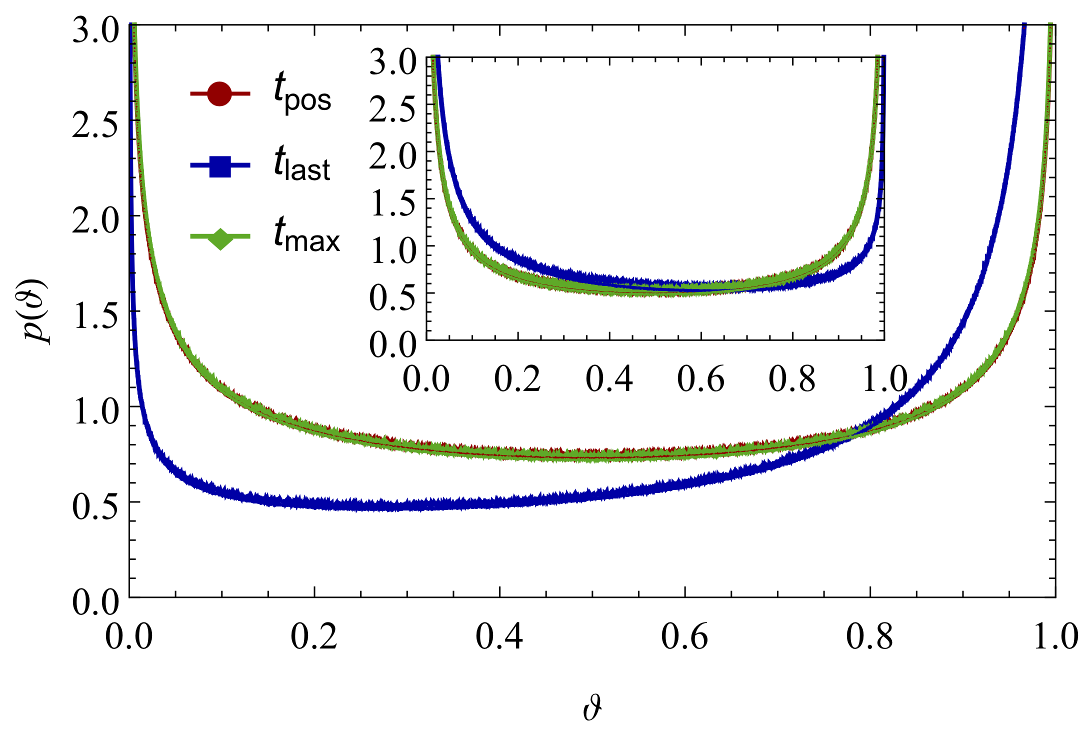
Figure 4: (color online) Numerical simulation results for the probability of the three observables $t_{\rm last}$, $t_{\rm max}$, and $t_{\rm pos}$ for an fBm with $H=0.33$. The inset shows the probabilities for $H=0.66$. Note that the distributions of $t_{\rm pos}$ and $t_{\rm max}$ are almost indistinguishable.

This is the simplest form we found. Alternative expressions were given in [60, 62, 61, 64], using that $\arctan(x)+\arctan\!\left(\frac{1}{x}\right)=\frac{\pi}{2}.$ Yet another equivalent form is given in Eq. (6) of [67]. We note that the expression (51b) is symmetric under $\vartheta\to 1-\vartheta$. This can be understood from the symmetry of the problem. We do not have an intuitive understanding of the equality of $\mathcal{F}_{1}^{\rm pos}$ and $\mathcal{F}_{1}^{\rm max}$, while the vanishing of $\mathcal{F}_{1}^{\rm last}$ in Eq. (51c) can easily be understood from perturbation theory [64].

Expressions for the sub-leading terms ${\cal F}_{2}$ can be written as integrals, which are hard to evaluate analytically. For $t_{\text{last}}$, it is given up to an additive constant by

$${\cal F}^{\rm last}_{2}(\vartheta)= \int_{0}^{\infty}\frac{dy_{1}dy_{2}}{y_{1}^{2}y_{2}^{2}}\;\Psi^{\rm last}\left(y_{1},y_{2},\frac{1-\vartheta}{\vartheta}\right),$$ (52a)

where $$\Psi^{\rm last}(y_{1},y_{2},z) (y_{1},y_{2})$$ is symmetric in and given by

$$\Psi^{\rm last}\left(y_{1},y_{2},z\right) =2\sqrt{(1+y_{1}+y_{2})z}$$

$$\times\Big{(} 1-\sqrt{1+y_{1}}-\sqrt{1+y_{2}}+\sqrt{1+y_{1}+y_{2}}\Big{)}$$

$$\times\Big{(}\sqrt{z}\,-\, \Theta(z-y_{1})\sqrt{z-y_{1}}-\Theta(z-y_{2})\sqrt{z-y_{2}}$$

$$+\Theta(z-y_{1}-y_{2})\sqrt{z-y_{1}-y_{2}}\Big{)},$$ (52b)

with $$\Theta(x) {\cal F}_{2}^{\rm max} {\cal F}_{2}^{\rm pos}$$ being the Heaviside step function. Expressions for and are cumbersome and given later.

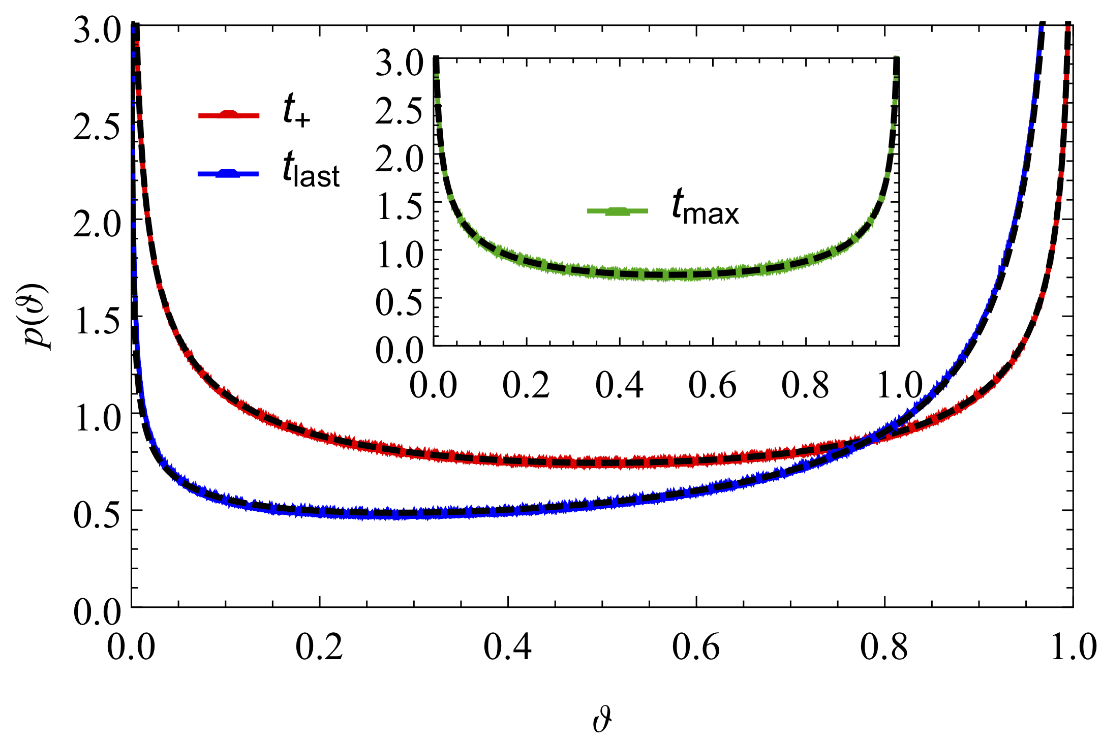
Figure 5: A comparison of the data shown in Fig. 4 with their theoretical formula (47)-(49). The dashed lines are for theoretical results. The distribution $p_{\rm max}(\vartheta)$ is shown in the inset as it is almost indistinguishable from the distribution $p_{\rm pos}(\vartheta)$.

In order that the reader can use our results, we give simple but rather precise approximations for the results obtained after numerical integration.

$${\cal F}_{2}^{\rm last}(\vartheta)\simeq -17.92401+13.30207\sqrt{\vartheta}$$ (53)

$$-2.16604\sqrt{1-\vartheta}+8.30059\vartheta+11.59529\vartheta^{\frac{3}{2}}$$ (54)

$$+13.23121(1-\vartheta)^{\frac{3}{2}}-10.74274\vartheta^{2},$$ (55)

$${\cal F}_{2}^{\rm max}(\vartheta)\simeq -0.431001+1.69259\left[\vartheta(1-\vartheta)\right]^{\frac{1}{2}}$$ (56)

$$-1.93367\left[\vartheta(1-\vartheta)\right]+1.3572\left[\vartheta(1-\vartheta)\right]^{\frac{3}{2}}$$

$$-0.33995\left[\vartheta(1-\vartheta)\right]^{2},$$ (57)

$${\cal F}_{2}^{\rm pos}(\vartheta)\simeq -0.842235+1.76479\left[\vartheta(1-\vartheta)\right]^{\frac{1}{2}}$$ (58)

$$+3.70810\left[\vartheta(1-\vartheta)\right]-9.71973\left[\vartheta(1-\vartheta)\right]^{\frac{3}{2}}$$ (59)

$$+7.40511\left[\vartheta(1-\vartheta)\right]^{2}.$$ (60)

These approximate functions are estimated respecting symmetries in the problem, i.e. that ${\cal F}_{2}^{\rm pos}(\vartheta)$ and ${\cal F}_{2}^{\rm max}(\vartheta)$ are symmetric under the exchange of $\vartheta\rightarrow 1-\vartheta$ while ${\cal F}_{2}^{\rm last}(\vartheta)$ is not.

• We stated above that $p_{\rm pos}(\vartheta)$ and $p_{\rm max}(\vartheta)$ are symmetric around $\vartheta=\frac{1}{2}$, while $p_{\rm last}(\vartheta)$ is not (except for $H=\frac{1}{2}$). Symmetry of the first two probabilities is due to the observation that $x_{t}$ and $X_{T}-x_{T-t}$ have the same law. For $p_{\rm last}$ the asymmetry is easy to see from the almost-straight-line trajectories for $H\simeq 1$ in Fig. 1, which makes $\vartheta=0$ the most probable value. This is reflected in the small-$\vartheta$ divergence of the distribution (47) in the limit of $H\to 1$.

IV.1 Comparison with numerical results

An efficient implementation of fBm on a computer is non-trivial due to its long-range correlations in time. For this paper, we use the Davis-Harte algorithm [70, 71], which generates sample trajectories drawn from a Gaussian probability with covariance (1) in a time of order $N\ln(N)$, given $N$ equally spaced discretization points. Details of this algorithm are given in App. D. Interestingly, for the first-passage time, recently an algorithm was introduced which grows as $\ln(N)^{3}$, albeit accepting a small error probability [66, 72, 73], allowing for even more precise estimates.

Results for the three probabilities from our computer simulations are shown in figure 4 for $H=0.33$. They are obtained by averaging over $5\times 10^{9}$ sample trajectories, each generated with $2^{13}$ discrete-time steps. The two distributions $p_{\rm max}(\vartheta)$ and $p_{\rm pos}(\vartheta)$ are almost indistinguishable, as predicted in their theoretical expressions in Eqs. (48) and (49).

            $H=0.5$

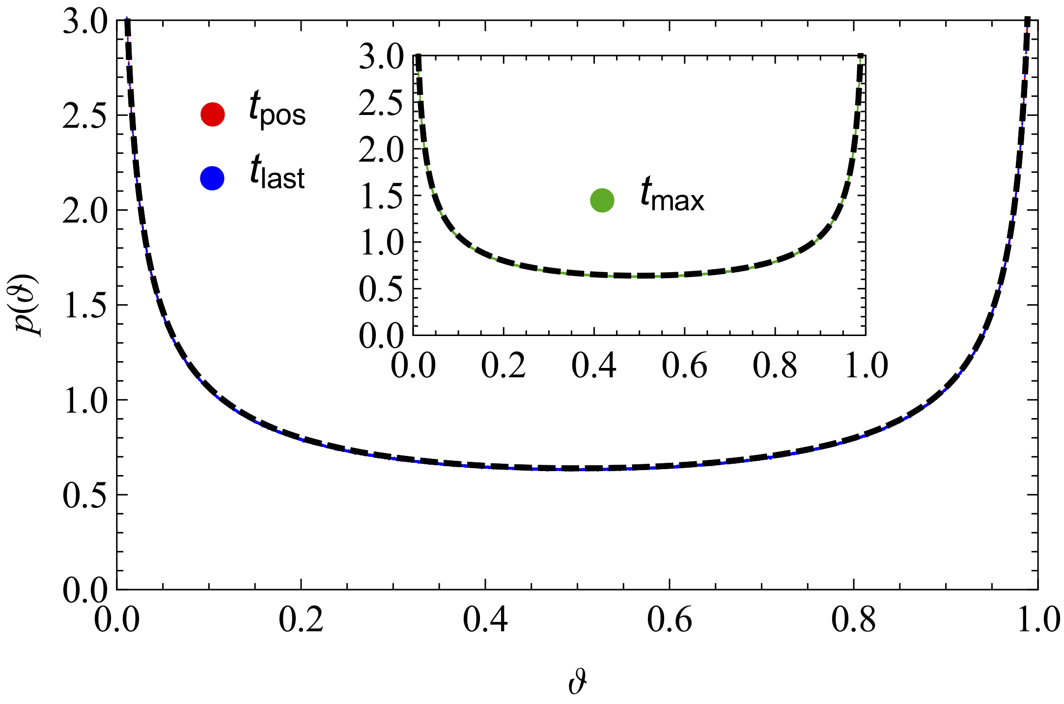
            $H=0.6$

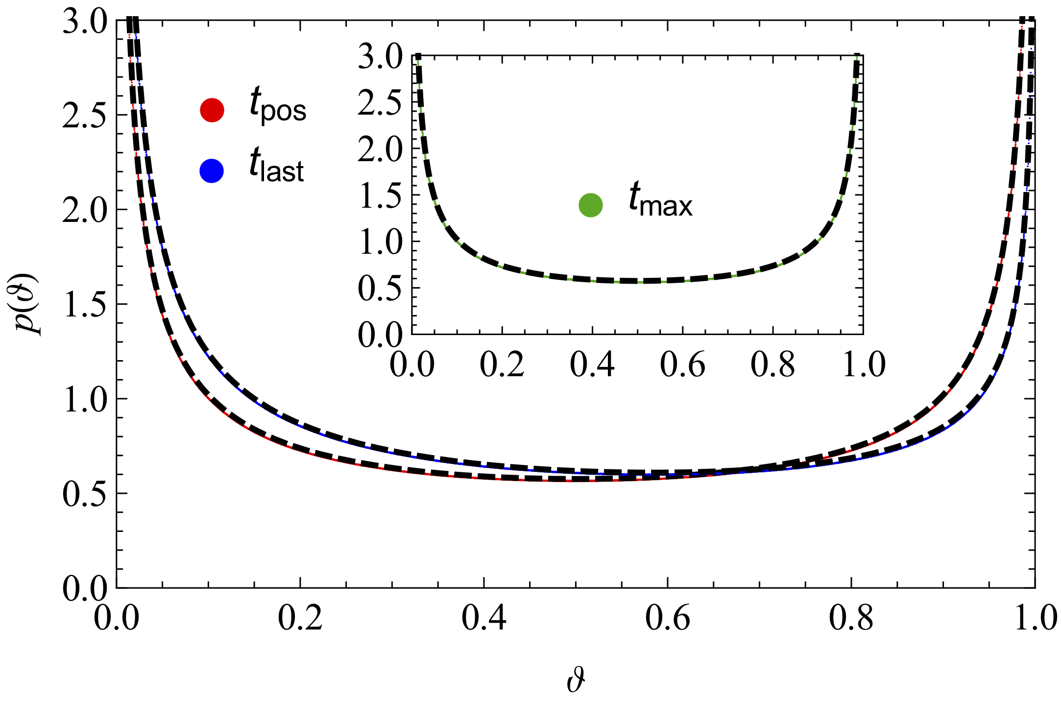
            $H=0.75$

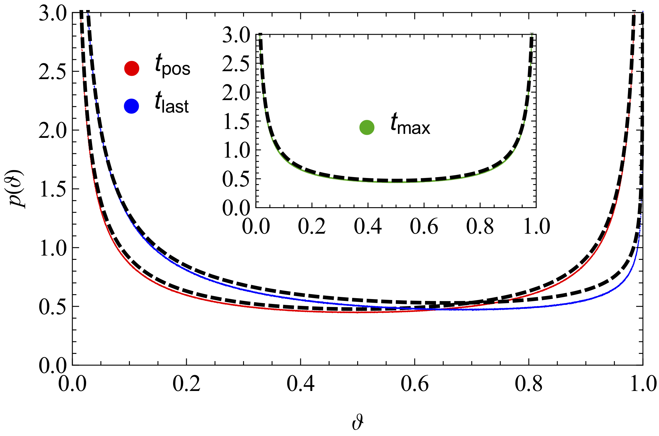
            $H=0.9$

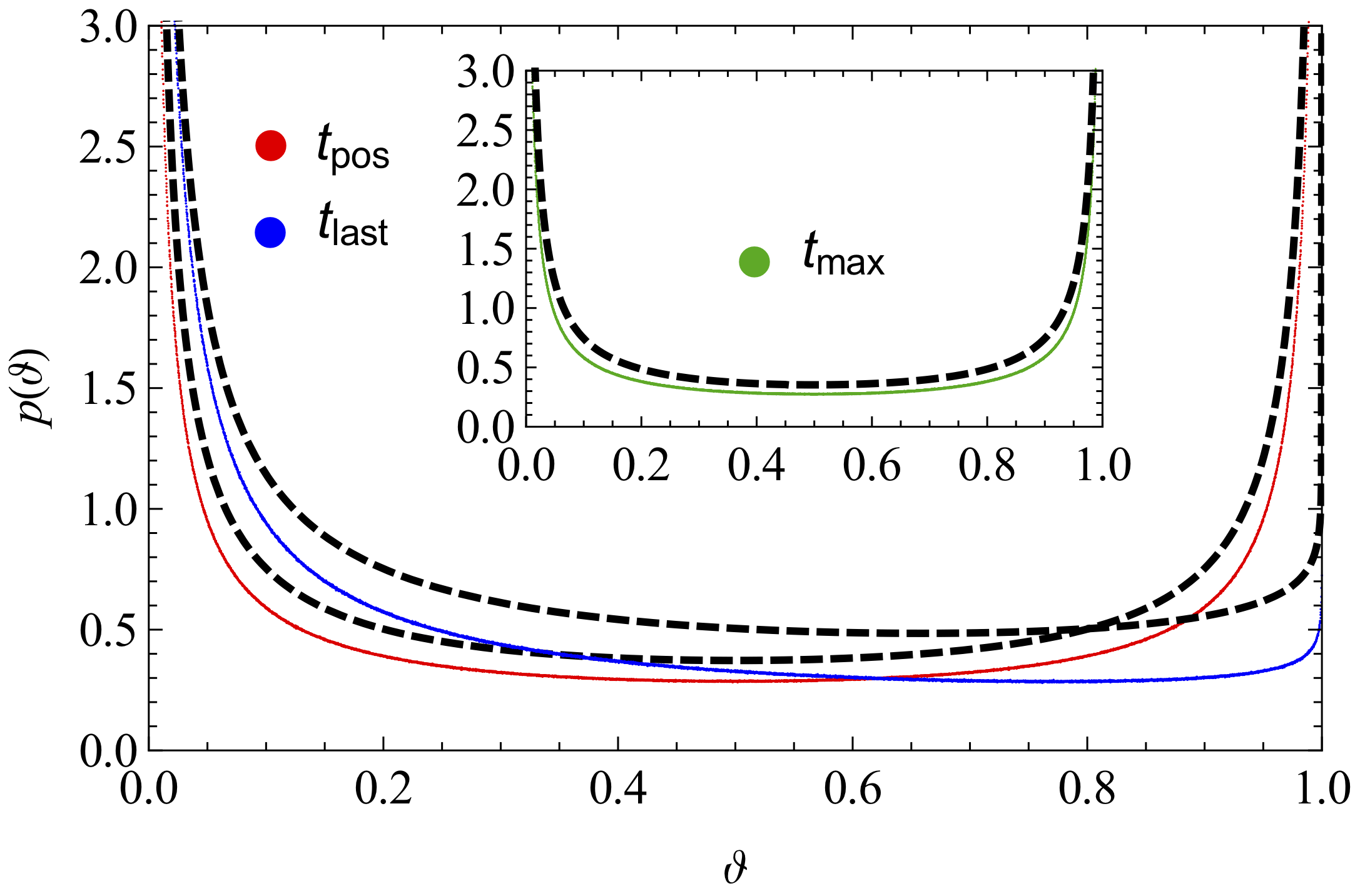
Figure 6: A comparison of the theoretical formulas in Eqs. (47)-(49) with their corresponding numerical simulation result of an fBm at diffrent values of $H\geq\frac{1}{2}$: $H=0.5$, $0.6$, $0.75$ and $0.9$. The dashed lines are the theoretical results, the continuous lines the numerical results.

Figure 4 also shows that $p_{\rm last}(\vartheta)$ behaves markedly differently from the other two distributions; especially, it is asymmetric under the exchange $\vartheta\to 1-\vartheta$. This asymmetry in exponents is reversed around $H=\tfrac{1}{2}$, as shown in the inset of figure 4. This can be seen in the scaling form in Eq. (47).

A comparison of numerical data for $H=0.33$ with their corresponding theoretical result in Eqs. (47)-(49) are shown in Fig. 5. They are in excellent agreement. Deviations are visible for higher values of $H$ as shown in Fig. 6 for a set of increasing values of $H\geq\frac{1}{2}$. We see a perfect agreement between theoretical and numerical results for $H=\frac{1}{2}$, (i.e. $\varepsilon=0$). The agreement is very good for small $\varepsilon=H-\tfrac{1}{2}$, but deviations can be seen as $\varepsilon$ is increased beyond $|\varepsilon|\approx 0.25$, i.e. $H\leq 0.25$ or $H\geq 0.75$.

The difference between $p_{\rm last}$ and $p_{\rm max}$ first appears in the second-order term $\mathcal{F}_{2}$ in Eq. (50). In Fig. 7 we plot our theoretical results of ${\cal F}_{2}(\vartheta)$ alongside the results from computer simulations. This give a finer verification of our theory. To illustrate this procedure, we use Eq. (49) to define

$${\cal F}_{2,\varepsilon}^{\rm pos}(\vartheta):=\frac{1}{\varepsilon}\left[\frac{1}{\varepsilon}\ln\!\bigg{(}p_{\rm pos}(\vartheta)\frac{[\vartheta(1-\vartheta)]^{H}}{\cal N}\bigg{)}-{\cal F}_{1}^{\rm pos}(\vartheta)\right].$$ (61)

Then, ${\cal F}_{2,\varepsilon}^{\rm pos}(\vartheta)={\cal F}_{2}^{\rm pos}(\vartheta)+{\cal O}(\varepsilon)$ and it contains all terms in the exponential in Eq. (49) except ${\cal F}_{1}^{{\rm pos}}(\vartheta)$. We can further improve this estimate by observing that the sub-leading term in ${\cal F}_{2,\varepsilon}^{\rm pos}(\vartheta)$ is odd in $\varepsilon$. Define

$$\overline{\cal F}_{2,\varepsilon}^{\rm pos}(\vartheta):=\frac{1}{2}\Big{[}{\cal F}_{2,\varepsilon}^{\rm pos}(\vartheta)+{\cal F}_{2,-\varepsilon}^{\rm pos}(\vartheta)\Big{]},$$ (62)

then $\overline{\cal F}_{2,\varepsilon}^{\rm pos}(\vartheta)$ differs from the theoretical ${\cal F}_{2}^{\rm pos}(\vartheta)$ by order $\varepsilon^{2}$ or higher, for small $\varepsilon$, equivalent to an order $\varepsilon^{4}$ correction to $p_{\rm last}(\vartheta)$.

A comparison of $\overline{\cal F}_{2,\varepsilon}^{\rm pos}(\vartheta)$ extracted from numerical simulations of $p_{\rm pos}(\vartheta)$ to the theoretical result of ${\cal F}_{2}^{\rm pos}(\vartheta)$ is shown in Fig. 7 for $\varepsilon=\pm\frac{1}{6}$ (i.e. for $H=\frac{2}{3}$ and $\frac{1}{3}$). The figure also contains a similar comparison for ${\cal F}_{2}^{\rm last}(\vartheta)$ and ${\cal F}_{2}^{\rm max}(\vartheta)$, with their corresponding numerical results. One sees the excellent agreement between results from our theory and numerical simulations. We remind that these are sub-sub-leading corrections, almost indiscernible in the probability density $p(\vartheta)$ shown on Fig. 5.

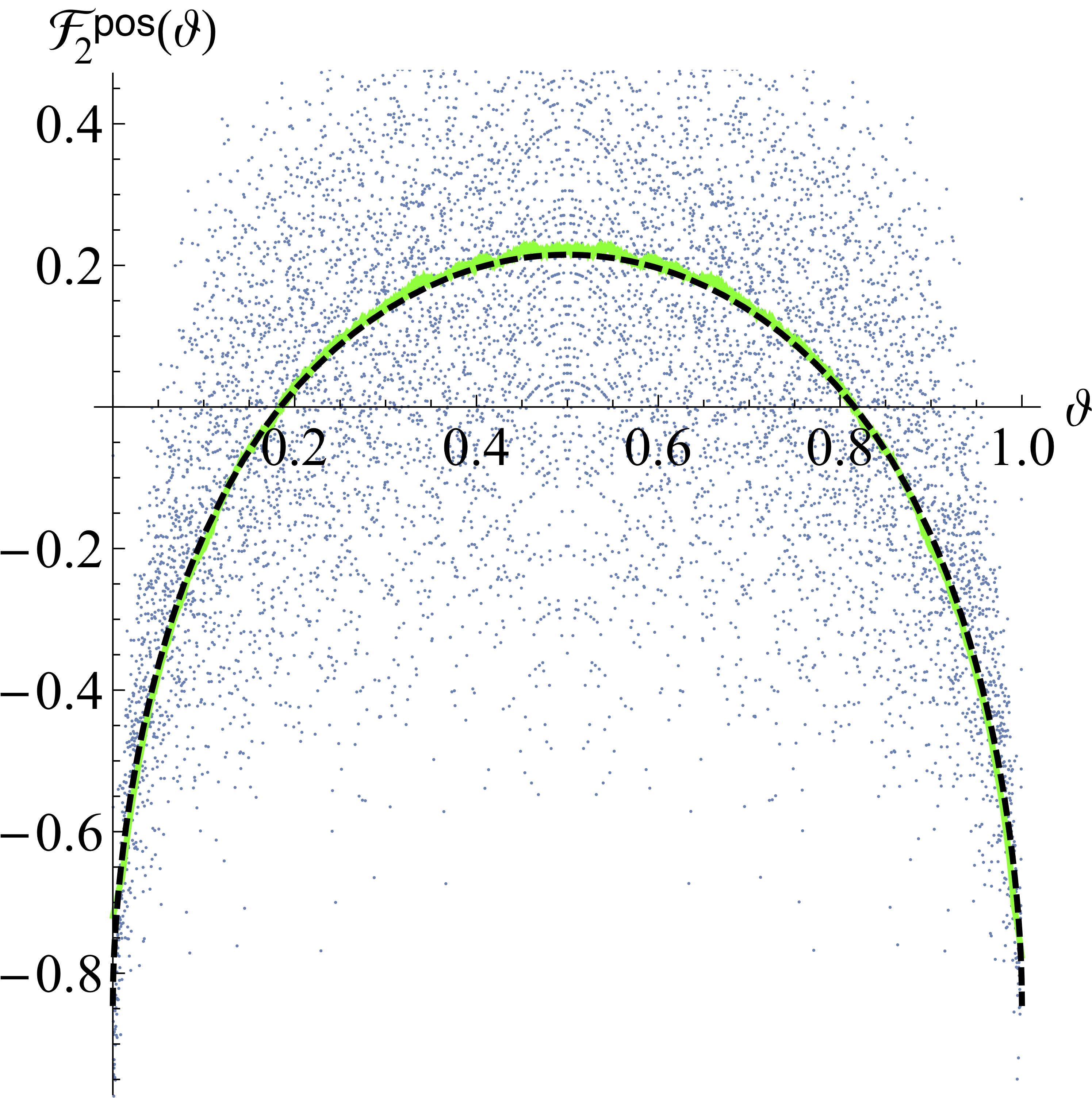
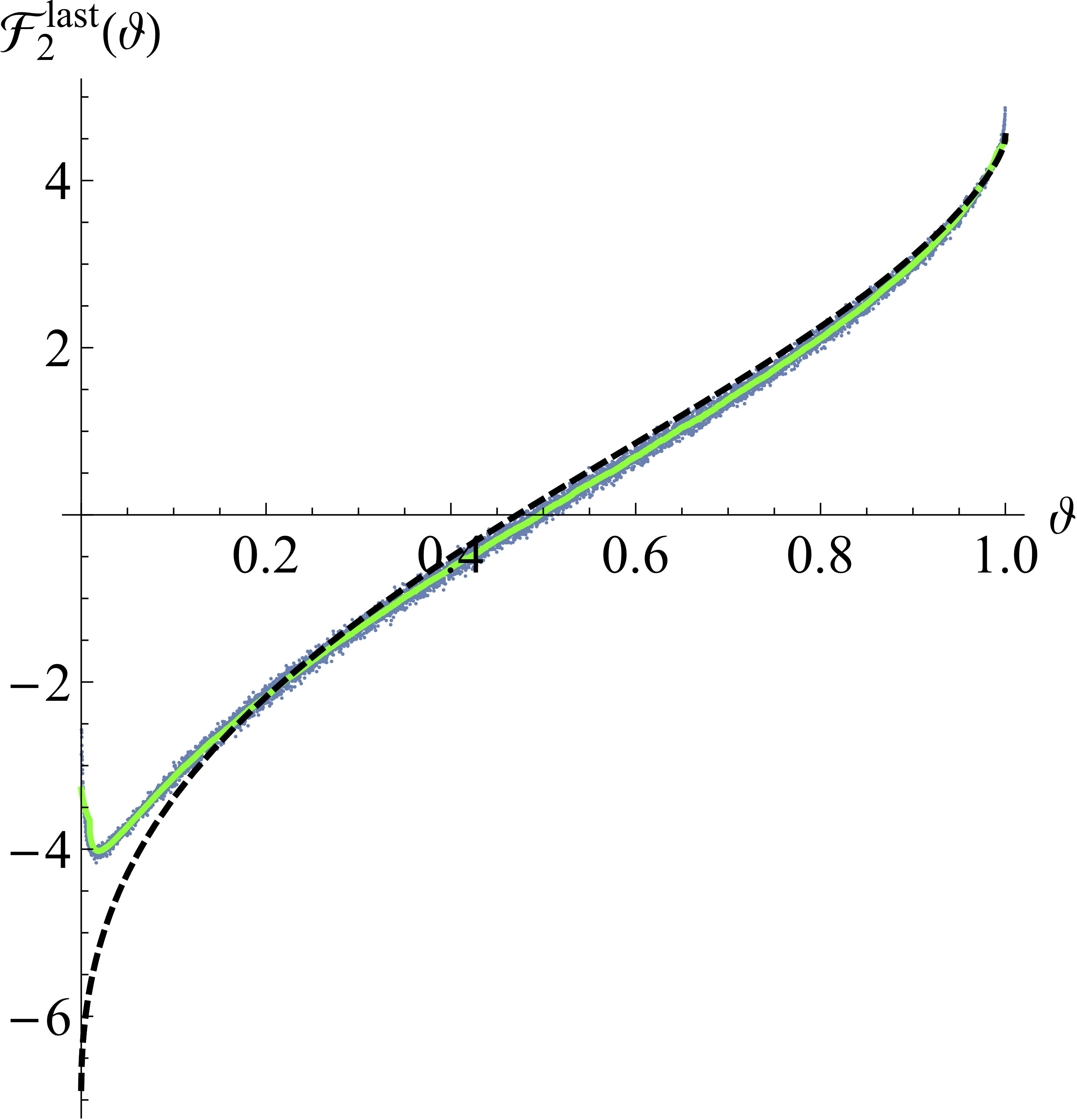
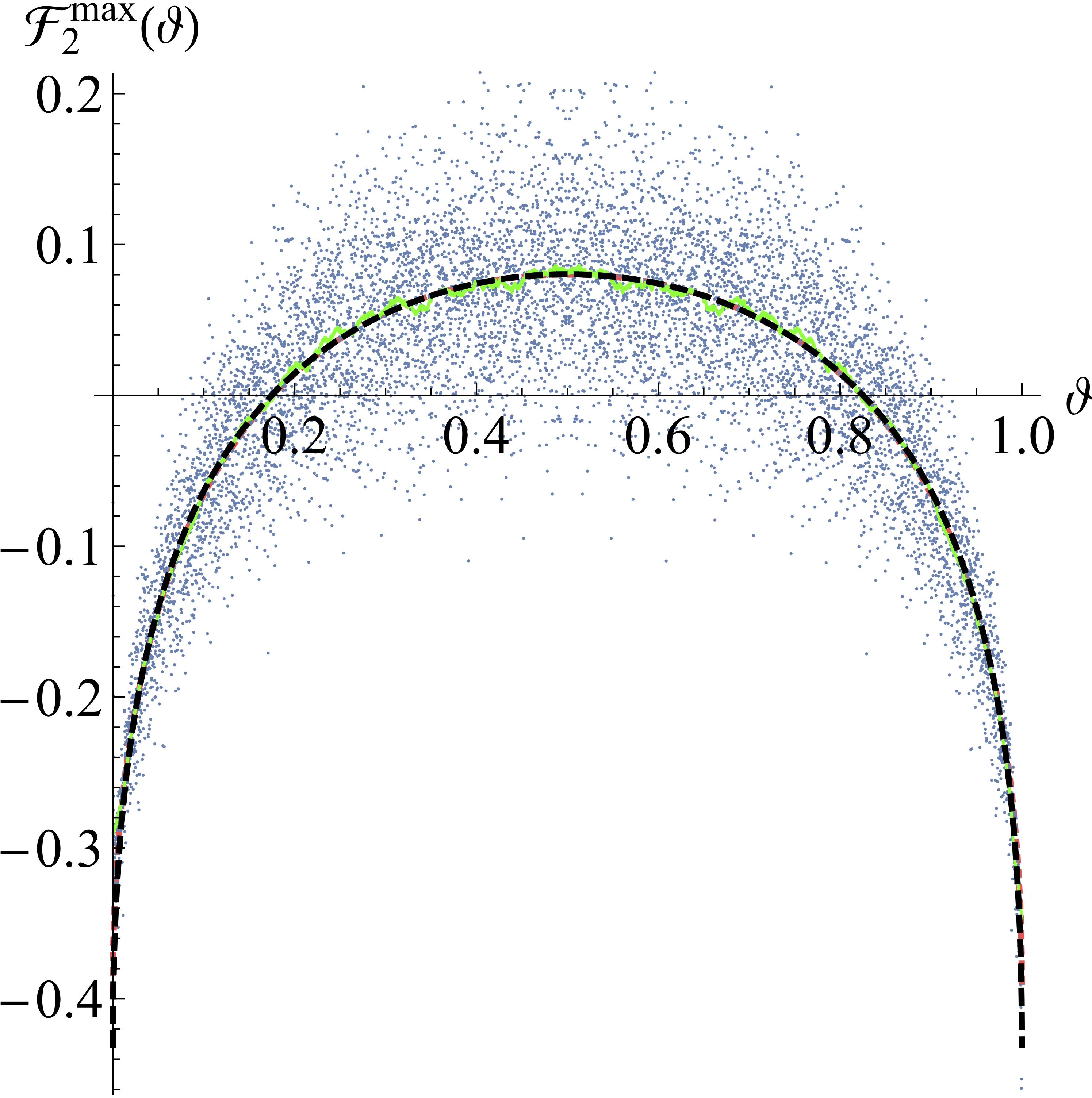
Figure 7: A comparison of the three ${\cal F}_{2}(\vartheta)$ obtained analytically (black dashed lines) and their measurement using formula (62) with $\varepsilon=\pm\tfrac{1}{6}$. From left to right: $(a)$ positive time, $(b)$ time for the last visit to the origin, and $(c)$ time for the maximum. The scattered dots are the raw data from trajectories of $N=2^{13}$ time steps, averaged over $5\times 10^{9}$ samples, which are coarse grained by a factor of 100 to give the green curve.

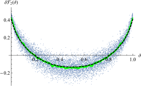
Figure 8: The difference $\delta{\cal F}_{2}(\vartheta)={\cal F}_{2}^{\rm max}(\vartheta)-{\cal F}_{2}^{\rm pos}(\vartheta)$ using the same conventions as in Fig. 7. This plot quantifies the difference between the distribution of $t_{\rm max}$ and $t_{\rm pos}$.

An important observation from Fig. 7 is that for all three observables $\mathcal{F}_{2}(\vartheta)$ is finite in the entire range of $\vartheta$. We note that the amplitude of ${\cal F}_{2}^{\rm last}(\vartheta)$ is about ten times larger than ${\cal F}_{2}^{\rm pos}(\vartheta)$ and ${\cal F}_{2}^{\rm max}(\vartheta)$. The former also shows the largest deviations from our theoretical result, especially for $\vartheta\to 0$. These indicate the presence of sub-leading terms of order $\varepsilon^{4}$, or higher in $p$.

The difference between $p_{\rm pos}(\vartheta)$ and $p_{\rm max}(\vartheta)$ first appears at second order in perturbation theory. To underline that $\mathcal{F}_{2}^{\rm pos}(\vartheta)$ and $\mathcal{F}_{2}^{\rm max}(\vartheta)$ in Eqs. (57) and (60) are distinct functions, we show in Fig. 8 their difference

$$\delta\mathcal{F}_{2}(\vartheta) = {\cal F}_{2}^{\rm max}(\vartheta)-{\cal F}_{2}^{\rm pos}(\vartheta)$$ (63)

$$= \lim_{\varepsilon\to 0}\frac{1}{\varepsilon^{2}}\ln\!\bigg{(}\frac{p_{\rm max}(\vartheta)}{p_{\rm pos}(\vartheta)}\Big{)}.$$ (64)

The theoretical result of the difference shows excellent agreement with the numerical data for $\overline{\cal F}_{2,\varepsilon}^{\rm max}(\vartheta)-\overline{\cal F}_{2,\varepsilon}^{\rm pos}(\vartheta)$ defined following the same conventions as in Eq. (62). This proves that the laws for $t_{\rm max}$ and $t_{\rm pos}$ are indeed different.

IV.2 Scaling analysis

The prefactor of the exponential in formula Eqs. (47)-(49) can be predicted using scaling arguments. The simplest one is $p_{\rm last}(\vartheta)$, which is the probability that the fBm is at the origin at time $\vartheta$ and does not return for the remaining time $1-\vartheta$. (We put the total time $T=1$, s.t. $\vartheta=t$.) The probability for the first part of the event scales as $\vartheta^{-H}$, see Eq. (18). The second part scales as $\vartheta^{-\theta}$, where $\theta=1-H$ is the persistent exponent [32, 33, 59]. Combining the two gives the prefactor in Eq. (47).

The scaling argument for $p_{\rm max}(\vartheta)$ is more involved, and was first discussed in Refs. [59, 62, 64]. One starts with the relation

$${\cal P}_{T}(m)=\frac{d\mathscr{S}_{T}(m)}{dm},$$ (65)

where ${\cal P}_{T}(m)$ is the probability for the position of the maximum $m$ for an fBm in a time interval $T$ started at the origin; $\mathscr{S}_{T}(m)$ is the survival probability up to time $T$ for an fBm started at $m>0$, in presence of an absorbing wall at the origin. Self-affinity of an fBm suggests the scaling form

$${\cal P}_{T}(m)=\frac{1}{T^{H}}g_{1}\!\left(\frac{m}{T^{H}}\right);\qquad\mathscr{S}_{T}(m)=g_{2}\!\left(\frac{m}{T^{H}}\right),$$ (66)

which leads to

$$g_{1}(x)=g_{2}^{\prime}(x).$$ (67)

To be consistent with the result for the persistence exponent [32, 33], one must have $g_{2}(x)\sim x^{\frac{\theta}{H}}$ for small $x$. This leads to $g_{1}(x)\sim x^{\frac{\theta}{H}-1}$, equivalent to

$${\cal P}_{T}(m)\sim\frac{m^{\frac{\theta}{H}-1}}{T^{\theta}}\qquad\textrm{for small {\hbox{m}}.}$$ (68)

To relate to the distribution $P_{T}(t_{\rm max})$ of $t_{\rm max}$ we use that at small $t_{\rm max}$ the maximum $m$ is also small and $m\sim t_{\rm max}^{H}$. This leads to

$$P_{T}(t_{\rm max})={\cal P}_{T}(m)\frac{dm}{dt_{\rm max}}\sim\frac{1}{t_{\rm max}}\left(\frac{t_{\rm max}}{T}\right)^{\!\!\theta}.$$ (69)

Substituting $\theta=1-H$ one gets

$$P_{T}(t_{\rm max})\sim\frac{1}{T}\left(\frac{t_{\rm max}}{T}\right)^{\!\!-H},$$ (70)

and equivalently

$$p_{\rm max}(\vartheta)=T\,P_{T}(\vartheta\,T)\sim{\vartheta^{-H}}\qquad\textrm{for small {\hbox{\vartheta}}.}$$ (71)

Using the symmetry of the probability $p_{\rm max}(\vartheta)$ under $\vartheta\to 1-\vartheta$ one gets $(1-\vartheta)^{-H}$ for $\vartheta\rightarrow 1$. This gives the prefactor in Eq. (48).

A similar argument relating to the persistent exponent [74] can be constructed for the distribution of $t_{\rm pos}$. For $t_{\rm pos}\ll T$, probability $P_{T}(t_{\rm pos})$ for an fBm to remain positive of net $t_{\rm pos}$ time, relates to persistence probability for the fBm to stay negative for most of its total duration $T$. This means, for $1\ll t_{\text{pos}}\ll T$,

$$P_{T}(t_{\rm pos})\sim T^{-\theta},$$ (72)

with the persistent exponent $\theta$. For this $T$-dependence to be consistent with the re-scaled probability $P_{T}(\vartheta\,T)=\frac{1}{T}p_{\rm pos}(\vartheta)$, one must have

$$p_{\rm pos}(\vartheta)\sim\vartheta^{\theta-1}\qquad\text{for {\hbox{\vartheta\to 0}},}$$ (73)

giving the small $\vartheta$ divergence in Eq. (49). The symmetry under $\vartheta\to 1-\vartheta$ gives the divergence near $\vartheta\to 1$.

IV.3 Comparison to an exact result

In Ref. [12] the first few moments of $t_{\rm pos}$ were calculated analytically for an fBm of $H=\frac{1}{4}$. It is straightforward to generalize this analysis for arbitrary $H$. For the fraction of positive time $\vartheta={t_{\rm pos}}/{T}$, we obtain the first three moments: $\langle\vartheta\rangle=\frac{1}{2}$ (obvious from the symmetry of the distribution),

$$\langle\vartheta^{2}\rangle =\frac{1}{4}+\frac{1}{2\pi}\int_{0}^{1}dr\,\arcsin R(r),$$ (74a)

$$\langle\vartheta^{3}\rangle =\frac{1}{8}+\frac{3}{4\pi}\int_{0}^{1}dr\,\arcsin R(r),$$ (74b)

where

$$R(r)=\frac{1}{2r^{H}}\left[1+r^{2H}-(1-r)^{2H}\right].$$ (74c)

It is hard to determine higher moments. The problem maps to the orthant probability problem for a multivariate Gaussian, which is still unsolved [75].

A perturbation expansion of Eq. (74c) in $\varepsilon=H-\frac{1}{2}$ gives

$$\langle\vartheta^{2}\rangle =\frac{3}{8}+\frac{\varepsilon}{4}\left(\ln 4-1\right)+\frac{\varepsilon^{2}}{24}\left(6\ln^{2}4-\pi^{2}\right)+\cdots,$$ (75a)

$$\langle\vartheta^{3}\rangle =\frac{5}{16}+\frac{3\varepsilon}{8}\left(\ln 4-1\right)+\frac{\varepsilon^{2}}{16}\left(6\ln^{2}4-\pi^{2}\right)+\cdots.$$ (75b)

Terms up to linear order are reproduced using our perturbation result Eq. (49). The $\varepsilon^{2}$ order terms ($0.0693$ for $\langle\vartheta^{2}\rangle$ and $0.1040$ for $\langle\vartheta^{3}\rangle$) obtained using the numerical approximation Eq. (60) agree with the exact result in Eq. (75) up to the third decimal place. (This is a $0.2\%$ disagreement, as apposed to a $40\%$ disagreement if $\mathcal{F}_{2}^{\rm pos}$ is ignored in Eq. (50c).)

A comparison of the exact result for the moments with their results obtained using Eq. (49) is shown in Fig. 9.

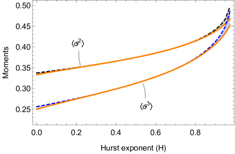
Figure 9: Second and third moment for the fraction of positive time $\vartheta=t_{\rm pos}/T$ as a function of the Hurst exponent $H$. The solid lines are the exact result in Eq. (74c), whereas the dashed lines denote their result obtained using Eq. (49) with $\mathcal{F}^{\rm pos}$ in Eq. (50) up to second order. The difference is noticeable for $H$ far from $\frac{1}{2}$, indicating corrections from higher-order terms in Eq. (50).

V Overview of theoretical analysis

Before we present details of the derivation for Eqs. (47)-(49), we give an overview of our approach. Our calculation is done using a double Laplace transformation $\mathcal{D}$ for the probability $P_{T}(\tau)$, defined by

$$\widetilde{P}(\lambda,s) = \mathscr{D}_{\begin{subarray}{c}\tau\to\lambda\\ T\to s\end{subarray}}\odot P_{T}(\tau),\qquad\text{with}$$ (76)

$$\mathscr{D}_{\begin{subarray}{c}\tau\to\lambda\\ T\to s\end{subarray}}\odot P_{T}(\tau) := \int_{0}^{\infty}dT\int_{0}^{T}d\tau\;e^{-sT-\lambda\tau}\;P_{T}(\tau).\qquad$$ (77)

For the re-scaled probability $p(\vartheta):=T\,P_{T}(\vartheta\,T)$ and it’s Laplace transform

$$\widetilde{p}(\kappa)=\int_{0}^{\infty}d\vartheta\,e^{-\kappa\,\vartheta}p(\vartheta),$$ (78)

the $\mathscr{D}$-transformation gives

$$\widetilde{P}(\lambda,s)=\frac{1}{s}\widetilde{p}\left(\frac{\lambda}{s}\right),~{}~{}\text{with}~{}~{}\widetilde{p}\left(\kappa\right)=\int_{0}^{1}d\vartheta\,\frac{p(\vartheta)}{1+\kappa\,\vartheta}.$$ (79)

Complex analysis using the residue theorem gives the corresponding inverse transformation (see App. E for a derivation),

$$p(\vartheta)=\frac{1}{2\pi i}\lim_{\delta\rightarrow 0^{+}}\frac{\widetilde{p}(-\frac{1}{\vartheta}-i\delta)-\widetilde{p}(-\frac{1}{\vartheta}+i\delta)}{\vartheta}.$$ (80)

Equivalently, one can write

$$p(\vartheta)=\frac{1}{2\pi i}\lim_{\phi\to\pi^{-}}\Big{[}\kappa\,\widetilde{p}(\kappa)-\kappa^{\star}\widetilde{p}(\kappa^{\star})\Big{]}_{\kappa=\frac{e^{i\phi}}{\vartheta}},$$ (81)

where the limit is taken from $\phi$ below $\pi$, and the star ($\star$) denotes complex conjugation.

The analysis can be simplified by considering the form of results in Eqs. (47)-(49) expected from scaling arguments. We write

$$p(\vartheta)=\frac{e^{\mathcal{F}(\vartheta,H)-(H-\frac{1}{2})\mathcal{R}(\vartheta)}}{\pi\sqrt{\vartheta(1-\vartheta)}}$$ (82)

with $\mathcal{R}(\vartheta)=\ln\tfrac{\vartheta}{(1-\vartheta)}$ for $t_{\rm last}$ and $\mathcal{R}(\vartheta)=\ln\vartheta(1-\vartheta)$ for $t_{\rm max}$ and $t_{\rm pos}$. (In writing Eq. (82) the normalization constant $\mathcal{N}$ from Eqs. (47)-(49) is absorbed in $\mathcal{F}$.) Then, from Eqs. (81) and (82) we write

$$\widetilde{p}(\kappa)=\frac{e^{\widetilde{\mathcal{F}}(\kappa,H)}}{\sqrt{1+\kappa}},$$ (83)

such that

$$e^{\mathcal{F}(\vartheta,H)-(H-\frac{1}{2})\mathcal{R}(\vartheta)}=\mathcal{K}_{\kappa\rightarrow\vartheta}^{-1}\odot e^{\widetilde{\mathcal{F}}(\kappa,H)}.$$ (84)

Here we define the transformation

$$\mathcal{K}_{\kappa\rightarrow\vartheta}^{-1}\odot f(\kappa)\equiv\lim_{\phi\rightarrow\pi-}\mathscr{R}\left[f\left(\frac{e^{i\phi}}{\vartheta}\right)\right],$$ (85)

with $\mathscr{R}$ denoting the real part.

In our derivation of the probabilities in Eqs. (47)-(49), we first calculate $\widetilde{\mathcal{F}}(\kappa,H)$, and then use Eq. (84) to obtain $\mathcal{F}(\vartheta,H)$. To do this order by order in a perturbation expansion in $\varepsilon=H-\frac{1}{2}$, write

$$\widetilde{\mathcal{F}}(\kappa,H)=\varepsilon\;\widetilde{\mathcal{F}}_{1}(\kappa)+\varepsilon^{2}\widetilde{\mathcal{F}}_{2}(\kappa)+\mathcal{O}(\varepsilon^{3}).$$ (86a)

Using this expansion in Eq. (84) we get Eq. (50) with

$$\mathcal{F}_{1}(\vartheta)= \,\mathcal{R}(\vartheta)+\mathcal{K}_{\kappa\rightarrow\vartheta}^{-1}\odot\widetilde{\mathcal{F}}_{1}(\kappa),$$ (86b)

$$\mathcal{F}_{2}(\vartheta)= -\frac{1}{2}\left[\mathcal{F}_{1}(\vartheta)-\mathcal{R}(\vartheta)\right]^{2}$$ (86c)

$$+\mathcal{K}_{\kappa\rightarrow\vartheta}^{-1}\odot\left[\widetilde{\mathcal{F}}_{2}(\kappa)+\frac{1}{2}\widetilde{\mathcal{F}}_{1}(\kappa)^{2}\right].$$ (86d)

• For completeness and for verification purposes, let us write the inverse transformation of Eq. (85),

  $$\mathcal{K}_{\vartheta\to k}\odot f(\vartheta):=\frac{1}{\pi}\int_{0}^{1}d\vartheta\;\frac{\sqrt{1+\kappa}}{1+\kappa\,\vartheta}\,\frac{f(\vartheta)}{\sqrt{\vartheta(1-\vartheta)}}.$$ (87)

  A list of the used inverse $\mathcal{K}$-transforms is given in App. F.

• From the normalization condition $\int_{0}^{1}d\vartheta\,p(\vartheta)=1$ one can see in Eq. (79) that $\widetilde{p}(0)=1$ and therefore in Eq. (83),

  $$\widetilde{\mathcal{F}}(\kappa,H)=0\qquad\text{for {\hbox{\kappa=0}}.}$$ (88)

• There are two reasons for performing our analysis using Laplace transform. The first is that convolutions in time are factorized, the second that integrations over space can be done over the Laplace-transformed propagator, but not the propagator in time. This will become clear in the analysis in the following sections.

VI Distribution of time $t_{\rm last}$ for the last visit to the origin

Figure 10: A schematic of an fBm trajectory contributing to the time $t_{\rm last}$ of last visit to the origin. The striped line indicates an absorbing boundary.

The analysis for the distribution of $t_{\rm last}$ is the simplest among the three observables, and we present it first. The probability of $t_{\rm last}=\tau$ for an fBm in a time window $[0,T]$ can be determined by

$$P_{T}(t_{\rm last}=\tau)=\frac{W(\tau,T)}{N(T)}\quad\text{for {\hbox{x_0\to 0}},}$$ (89)

where $W(\tau,T)$ is twice the weight of fBm trajectories that start at $X_{0}=0$, pass through $X_{\tau}=x_{0}>0$, and remain positive for the rest of the time (see Fig. 10 for an illustration). Note that the factor of $2$ accounts for the possibility that the final position is either $m>0$, or $m<0$. Here $N(T)$ is the normalization

$$N(T)=\int_{0}^{T}d\tau W(\tau,T).$$ (90)

(To keep notations simple, we avoid explicit reference to $x_{0}$, unless necessary.)

Formally, we write

$$W(\tau,T)= \,2\int\limits_{0}^{\infty}dm\int_{x(0)=0}^{x(T)=m}\mathcal{D}[x]\;\delta\big{(}x(\tau)-x_{0}\big{)}$$ (91)

$$\qquad\times\prod_{t=\tau}^{T}\Theta\big{(}x(t)\big{)}\;e^{-S}.$$ (92)

The perturbative expansion in Eq. (7) of the action leads to a similar expansion for $W$, given by

$$W(\tau,T)=W_{0}(\tau,T)+\varepsilon W_{1}(\tau,T)+\varepsilon^{2}W_{2}(\tau,T)+\ldots$$ (93)

with

$$W_{0}(\tau,T) =2\int_{0}^{\infty}dm\,\mathopen{\hbox{${\langle}$}\kern-2.72221pt\leavevmode\hbox{${\langle}$}}1\mathclose{\hbox{${\rangle}$}\kern-2.72221pt\leavevmode\hbox{${\rangle}$}}_{m},$$ (94)

$$W_{1}(\tau,T) =\int_{0}^{\infty}dm\,\mathopen{\hbox{${\Big{\langle}}$}\kern-2.72221pt\leavevmode\hbox{${\Big{\langle}}$}}\frac{S_{1}}{D}\mathclose{\hbox{${\Big{\rangle}}$}\kern-2.72221pt\leavevmode\hbox{${\Big{\rangle}}$}}_{m},$$ (95)

$$W_{2}(\tau,T) =\int_{0}^{\infty}dm\,\mathopen{\hbox{${\bigg{\langle}}$}\kern-2.72221pt\leavevmode\hbox{${\bigg{\langle}}$}}\frac{S_{1}^{2}}{4D^{2}}-2\frac{S_{2}}{D}\mathclose{\hbox{${\bigg{\rangle}}$}\kern-2.72221pt\leavevmode\hbox{${\bigg{\rangle}}$}}_{m}.$$ (96)

The double-angular brackets denote (for $m>0$) the average over trajectories as sketched in Fig. 10 with a standard Brownian measure,

$$\mathopen{\hbox{${\langle}$}\kern-2.72221pt\leavevmode\hbox{${\langle}$}}O[x]\mathclose{\hbox{${\rangle}$}\kern-2.72221pt\leavevmode\hbox{${\rangle}$}}_{m}:=\!\!\!\!\!\!\!\int\limits_{x(0)=0}^{x(T)=m}\mathcal{D}[x]\delta\big{(}x(\tau)-x_{0}\big{)}\prod_{t=\tau}^{T}\Theta\big{(}x(t)\big{)}\,e^{-\frac{S_{0}}{D}}O(x(t)).$$ (97)

This definition of double-angular brackets is specific to the trajectories used here, its definition in other sections will include the corresponding boundary conditions needed there.

VI.1 Zeroth order term

In terms of the free Brownian propagator Eq. (25) and the propagator in presence of an absorbing wall,

$$Z^{+}_{t}(x_{1},x_{2})=\int_{x(0)=x_{1}}^{x(t)=x_{2}}\mathcal{D}[x]\prod_{r=0}^{t}\Theta(x(r))e^{-\frac{S_{0}}{D}}$$ (98)

we write Eq. (94) as

$$W_{0}(\tau,T)=2\int_{0}^{\infty}dm\,Z_{\tau}(0,x_{0})\,Z^{+}_{T-\tau}(x_{0},m).$$ (99)

Its double Laplace transformation Eq. (77) denoted by

$$\widetilde{W}_{0}(\lambda,s)=\mathscr{D}_{\begin{subarray}{c}\tau\to\lambda\\ T\to s\end{subarray}}\odot W_{0}(\tau,T)$$ (100)

is

$$\widetilde{W}_{0}(\lambda,s)=2\int_{0}^{\infty}dm\,\widetilde{Z}_{s+\lambda}(0,x_{0})\;\widetilde{Z}^{+}_{s}(x_{0},m).$$ (101)

Here $\widetilde{Z}_{s}$ and $\widetilde{Z}_{s}^{+}$ are the Laplace transforms of $Z_{t}$ and $Z_{t}^{+}$, given by

$$\widetilde{Z}_{s}(x_{1},x_{2}) =\int_{0}^{\infty}dt\,e^{-st}\;Z_{t}(x_{1},x_{2})$$

$$=\frac{e^{-\sqrt{\frac{s}{D}}|x_{1}-x_{2}|}}{2\sqrt{sD}},$$ (102a)

and

$$\widetilde{Z}^{+}_{s}(x_{1},x_{2}) =\int_{0}^{\infty}dt\,e^{-st}\;Z^{+}_{t}(x_{1},x_{2})$$

$$=\frac{e^{-\sqrt{\frac{s}{D}}|x_{1}-x_{2}|}-e^{-\sqrt{\frac{s}{D}}|x_{1}+x_{2}|}}{2\sqrt{sD}}.$$ (102b)

Using these results in Eq. (101) and evaluating the integral for small $x_{0}$ we get, (see Eq. (430))

$$\widetilde{W}_{0}(s\,\kappa,s)\simeq\frac{x_{0}}{Ds}\times\frac{1}{\sqrt{1+\kappa}}.$$ (103)

• The factorization in Eq. (101) results from the identity

  $$\mathscr{D}_{\begin{subarray}{c}\tau\to\lambda\\ T\to s\end{subarray}}\odot\Big{[}g(\tau)f(T-\tau)\Big{]}=\widetilde{g}(s+\lambda)\;\widetilde{f}(s),$$ (104)

  where $\widetilde{g}(s)$ and $\widetilde{f}(s)$ are the Laplace transforms of $g(t)$ and $f(t)$, respectively.

• From Eq. (103) it is straightforward to verify the arcsine-law (4) for Brownian motion. One can use $D=1$ for $\varepsilon=0$ in Eq. (103), and verify that $W_{0}(\vartheta T,T)\simeq x_{0}[\pi T\sqrt{\vartheta(1-\vartheta)}]^{-1}$. Then, Eqs. (89) and (90) lead to the distribution (4).

VI.2 Linear order: 1-loop diagrams

Figure 11: One-loop diagrams: a graphical representation of the terms in Eq. (106a) for the linear order in our perturbation expansion. For all diagrams $r_{1}<r_{2}$, staying on the same side of $\tau$ as indicated. The dashed lines indicate coupling between points $r_{1}$ and $r_{2}$ with $r_{1}<r_{2}$ (indicated by an arrowhead) and a coupling strength $e^{y(r_{1}-r_{2})}$. The solid disks indicate the ‘charge’ $\dot{x}(r_{1})$ and $\dot{x}(r_{2})$ for the associated points. A similar convention will be used for diagrams in later parts of our analysis.

Using $S_{1}$ from Eq. (10a) we explicitly write Eq. (95) as

$$W_{1}(\tau,T)=\frac{1}{D}\int_{0}^{\infty} dm\int_{0}^{\Lambda}dy\int_{0}^{T}dr_{1}\int_{r_{1}}^{T}dr_{2}$$

$$\times e^{y(r_{1}-r_{2})}\;\mathopen{\hbox{${\big{\langle}}$}\kern-2.72221pt\leavevmode\hbox{${\big{\langle}}$}}\dot{x}(r_{1})\dot{x}(r_{2})\mathclose{\hbox{${\big{\rangle}}$}\kern-2.72221pt\leavevmode\hbox{${\big{\rangle}}$}}_{m}.$$ (105)

For convenience we use a graphical representation of the expression in Eq. (105). We write the amplitude in three parts, according to the relative order of times $r_{1}$, $r_{2}$, and $\tau$, as illustrated in the 1-loop diagrams in Fig. 11.

• Diagrams in Fig. 11 consists of couplings between a single pair of points, resulting in the $y$-integral in Eq. (105). In analogy with field theory, we refer to them as 1-loop diagrams, with $y$ representing the loop-variable to be integrated over. In Sec. VI.3, i.e. at second order, amplitudes involve couplings between two pairs, resulting into two $y$-integrations, and therefore referred to as 2-loop diagrams.

Following our convention for the diagrams in Fig. 11 we write Eq. (105) as

$$W_{1}=A_{1}+A_{2}+A_{3}$$ (106a)

with

$$A_{1}(\tau,T)=\frac{1}{D}\int\limits_{0}^{\infty}dm\int\limits_{0}^{\Lambda}dy\,J_{\tau}(0,x_{0};-y,y)\,Z^{+}_{T-\tau}(x_{0},m),$$ (106b)

$$A_{2}(\tau,T)=\frac{1}{D}\int\limits_{0}^{\infty}dm\int\limits_{0}^{\Lambda}dy\,Z_{\tau}(0,x_{0})\;J_{T-\tau}^{+}(x_{0},m;-y,y),$$ (106c)

$$A_{3}(\tau,T)$$

$$\!=\frac{1}{D}\int\limits_{0}^{\infty}dm\int\limits_{0}^{\Lambda}dy\,J_{\tau}(0,x_{0};-y)\;e^{-y\tau}J^{+}_{T{-}\tau}(x_{0},m;y).$$ (106d)

We defined

$$J_{t}(u,v;y_{1},\ldots,y_{n})$$

$$:=\int\limits_{0<r_{1}<\cdots<r_{n}}^{t}\prod_{i=1}^{n}\;e^{-y_{i}r_{i}}\int\limits_{x(0)=u}^{x(t)=v}\mathcal{D}[x]\dot{x}(r_{1})\cdots\dot{x}(r_{n})e^{-\frac{S_{0}}{D}}$$ (107)

and its analogue $J^{(+)}$ in presence of an absorbing wall at $x=0$. The integral over time in Eq. (107) is interpreted as in Eq. (15), i.e. with an ultraviolet cutoff $\Lambda$ on $y$.

Using Eq. (104) we write the double Laplace transform Eq. (77) of the diagrams $A_{i}$ in terms of Laplace transforms of $Z$ and $Z^{+}$ in Eq. (102), as well as Laplace transforms for $J$ and $J^{+}$. Expressions are obtained in App. N, and summarized here,

$$\widetilde{A}_{1}(\lambda,s)= \frac{1}{D}\int\limits_{0}^{\infty}dm\int\limits_{0}^{\Lambda}dy\,\widetilde{J}_{s+\lambda}(0,x_{0};-y,y)\;\widetilde{Z}^{+}_{s}(x_{0},m),$$

$$\widetilde{A}_{2}(\lambda,s)= \frac{1}{D}\int\limits_{0}^{\infty}dm\int\limits_{0}^{\Lambda}dy\,\widetilde{Z}_{s+\lambda}(0,x_{0})\;\widetilde{J}_{s}^{+}(x_{0},m;-y,y).$$

Using Eqs. (102), (466), and (475) gives, for small $x_{0}$,

$$\widetilde{A}_{1}(s\,\kappa,s) \simeq-\frac{x_{0}}{Ds}\times\frac{\widetilde{\mathcal{A}}(1+\kappa)}{\sqrt{1+\kappa}},$$

$$\widetilde{A}_{2}(s\,\kappa,s) \simeq\frac{x_{0}}{Ds}\times\frac{\widetilde{\mathcal{A}}(1)}{\sqrt{1+\kappa}},$$

with

$$\widetilde{\mathcal{A}}(z)= \int_{0}^{\Lambda/s}\frac{dy}{y^{2}}\left(\sqrt{z+y}-\sqrt{z}\right)^{2}.$$ (108)

A similar analysis for $A_{3}$ in Eq. (106d), using Eqs. (455) and (460), shows that the corresponding double Laplace transform $\widetilde{A}_{3}\sim x_{0}^{2}$, for small $x_{0}$. As a result, the double Laplace transform of $W_{1}(\tau,T)$ defined in analogy to Eq. (100) reads, for small $x_{0}$,

$$\widetilde{W}_{1}(s\,\kappa,s)\simeq\frac{x_{0}}{Ds}\times\frac{\widetilde{\mathcal{A}}(1)-\widetilde{\mathcal{A}}(1+\kappa)}{\sqrt{1+\kappa}}.$$ (109)

• The reason for $\widetilde{A}_{3}$ to vanish as $x_{0}^{2}$ or faster, for small $x_{0}$, can be understood from a simple observation. In the limit of $x_{0}\to 0$, $J_{t}(0,x_{0};y_{1},\ldots,y_{n})$ in Eq. (107) vanishes for odd $n$. One way to see this is by noting that, in the limit of $x_{0}\to 0$, for each trajectory with a certain $\dot{x}(r)$, there is a mirror trajectory $-\dot{x}(r)$, with equal probability. In comparison, $J^{+}(x_{0},m;y_{1},\ldots,y_{n})$ vanishes for $x_{0}\to 0$ because of the absorbing boundary. This means that in Eq. (106d), both $J$ and $J^{+}$ are at least of order $x_{0}$, and therefore $\widetilde{A}_{3}\sim x_{0}^{2}$, to the least. We shall see later that for a similar reason the amplitudes of the 2-loop diagrams $B$ and $C$ in Fig. 14 are of order $x_{0}^{2}$, for small $x_{0}$.

• We shall see that these diagrams $A_{1}$, $A_{2}$, and $A_{3}$ contribute to the propagator $W_{1}$ in Eq. (106a), thus to the scaling prefactor in Eq. (47), but they do not feed into the exponential term $\mathcal{F}^{\rm last}$.

VI.3 Quadratic order: 2-loop diagrams

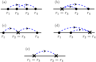
Figure 12: A diagramatic representation for the amplitude in Eq. (110) where all orders of time are allowed keeping $r_{2}>r_{1}$ and $r_{4}>r_{3}$ (as indicated by an arrowhead). We write the amplitude Eq. (110) in five parts according to the contraction of times (indicated by cross). In (a) none of the times are equal (contracted). In (b,c,d) two times are contracted and in (e) all four times are contracted.

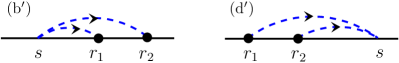
Figure 13: A diagramatic representation of the formula in Eq. (114) where for (b^′) $s<r_{1}<r_{2}$ and for (d^′) $r_{1}<r_{2}<s$.

Using Eq. (10) we explicitly write the terms in Eq. (96) as

$$\int_{0}^{\infty}dm\,\mathopen{\hbox{${\bigg{\langle}}$}\kern-2.72221pt\leavevmode\hbox{${\bigg{\langle}}$}}\frac{S_{1}^{2}}{4D^{2}}\mathclose{\hbox{${\bigg{\rangle}}$}\kern-2.72221pt\leavevmode\hbox{${\bigg{\rangle}}$}}_{m}$$ (110)

$$=\frac{1}{4D^{2}}\int\limits_{0}^{\infty}dm\int\limits_{0}^{\Lambda}dy_{1}dy_{2}\int\limits_{0}^{T}dr_{1}\int\limits_{r_{1}}^{T}dr_{2}\int\limits_{0}^{T}dr_{3}\int\limits_{r_{3}}^{T}dr_{4}\;$$ (111)

$$\qquad\times e^{y_{1}(r_{1}-r_{2})}\;e^{y_{2}(r_{3}-r_{4})}\mathopen{\hbox{${\Big{\langle}}$}\kern-2.72221pt\leavevmode\hbox{${\Big{\langle}}$}}\dot{x}(r_{1})\dot{x}(r_{2})\dot{x}(r_{3})\dot{x}(r_{4})\mathclose{\hbox{${\Big{\rangle}}$}\kern-2.72221pt\leavevmode\hbox{${\Big{\rangle}}$}}_{m}$$

and

$$\int_{0}^{\infty}dm\,\mathopen{\hbox{${\bigg{\langle}}$}\kern-2.72221pt\leavevmode\hbox{${\bigg{\langle}}$}} \frac{2S_{2}}{D}\mathclose{\hbox{${\bigg{\rangle}}$}\kern-2.72221pt\leavevmode\hbox{${\bigg{\rangle}}$}}_{m}=\frac{1}{D}\int\limits_{0}^{\infty}dm\int\limits_{0}^{\Lambda}dy_{1}dy_{2}$$ (112)

$$\times\int\limits_{0}^{T}dr_{1} \int\limits_{r_{1}}^{T}dr_{2}\bigg{[}\int\limits_{0}^{r_{1}}ds\;e^{-y_{1}(r_{1}-s)-y_{2}(r_{2}-s)}$$ (113)

$$+\int\limits_{r_{2}}^{T}ds \;e^{-y_{1}(s-r_{1})-y_{2}(s-r_{2})}\bigg{]}\mathopen{\hbox{${\Big{\langle}}$}\kern-2.72221pt\leavevmode\hbox{${\Big{\langle}}$}}\dot{x}(r_{1})\dot{x}(r_{2})\mathclose{\hbox{${\Big{\rangle}}$}\kern-2.72221pt\leavevmode\hbox{${\Big{\rangle}}$}}_{m}.\qquad$$ (114)

A graphical illustration of the amplitudes in Eq. (110) and Eq. (114) is shown in Figs. 12 and 13. Similar to the conventions in Fig. 11, a dashed line indicates an interaction between points $r_{i}$ and $r_{j}$ with an amplitude $e^{y(r_{i}-r_{j})}$. The solid disks indicate the field derivative $\dot{x}(r_{i})$ at point $r_{i}$. For a contracted point, indicated by a cross, the associated amplitude is $2D$. A reason for this will be clear shortly. Empty points in Fig. 13 have an amplitude 1.

We shall see that among these diagrams, only diagrams (a) and (c) contribute at the second order. This can be directly seen using the normal-ordered weight in Eq. (16). Here, we explicitly show why this happens.

We find that the amplitudes of diagrams (b) and (b^′) are equal, as are those of (d) and (d^′). To see this we use that under Wick contraction between $\dot{x}(r_{1})$ and $\dot{x}(r_{3})$

$$\mathopen{\hbox{${\Big{\langle}}$}\kern-2.72221pt\leavevmode\hbox{${\Big{\langle}}$}}\dot{x}(r_{1})\dot{x}(r_{2})\dot{x}(r_{3})\dot{x}(r_{4})\mathclose{\hbox{${\Big{\rangle}}$}\kern-2.72221pt\leavevmode\hbox{${\Big{\rangle}}$}}_{m}\to 2D\;\mathopen{\hbox{${\Big{\langle}}$}\kern-2.72221pt\leavevmode\hbox{${\Big{\langle}}$}}\dot{x}(r_{2})\dot{x}(r_{4})\mathclose{\hbox{${\Big{\rangle}}$}\kern-2.72221pt\leavevmode\hbox{${\Big{\rangle}}$}}_{m}.$$ (115)

(A similar result holds for contraction of any pair of times.) One can see this as a consequence of $\delta(r_{i}-r_{j})$ term in Eq. (447), and its analogue in presence of an absorbing boundary. Using the result (115) in Eq. (110) for diagram (b) we write its amplitude as

$$\frac{1}{2D}\int_{0}^{\infty}dm\int_{0}^{\Lambda}dy_{1}dy_{2}\int_{0}^{T}dr_{1}\int_{r_{1}}^{T}dr_{2}\int_{r_{1}}^{T}dr_{4}$$

$$\qquad\qquad\times e^{y_{1}(r_{1}-r_{2})}e^{y_{2}(r_{1}-r_{4})}\mathopen{\hbox{${\Big{\langle}}$}\kern-2.72221pt\leavevmode\hbox{${\Big{\langle}}$}}\dot{x}(r_{2})\dot{x}(r_{4})\mathclose{\hbox{${\Big{\rangle}}$}\kern-2.72221pt\leavevmode\hbox{${\Big{\rangle}}$}}_{m}$$

$$=\frac{1}{D}\int_{0}^{\infty}dm\int_{0}^{\Lambda}dy_{1}dy_{2}\int_{0}^{T}dr_{2}\int_{r_{2}}^{T}dr_{4}\int_{0}^{r_{2}}dr_{1}$$

$$\qquad\qquad\times e^{y_{1}(r_{1}-r_{2})}e^{y_{2}(r_{1}-r_{4})}\mathopen{\hbox{${\Big{\langle}}$}\kern-2.72221pt\leavevmode\hbox{${\Big{\langle}}$}}\dot{x}(r_{2})\dot{x}(r_{4})\mathclose{\hbox{${\Big{\rangle}}$}\kern-2.72221pt\leavevmode\hbox{${\Big{\rangle}}$}}_{m}.$$

Following a relabeling of the dummy variables $r$ we see that the integral is equal to the amplitude of diagram (b^′) from Eq. (114) and Fig. 13. A similar analysis shows equal amplitude for diagrams (d) and (d^′).

The amplitude of diagram (e), where all four times are contracted, is proportional to $W_{0}$ in Eq. (94), which can be seen by using

$$\mathopen{\hbox{${\Big{\langle}}$}\kern-2.72221pt\leavevmode\hbox{${\Big{\langle}}$}}\dot{x}(r_{1})\dot{x}(r_{2})\dot{x}(r_{3})\dot{x}(r_{4})\mathclose{\hbox{${\Big{\rangle}}$}\kern-2.72221pt\leavevmode\hbox{${\Big{\rangle}}$}}_{m}\to 4D^{2}\mathopen{\hbox{${\langle}$}\kern-2.72221pt\leavevmode\hbox{${\langle}$}}1\mathclose{\hbox{${\rangle}$}\kern-2.72221pt\leavevmode\hbox{${\rangle}$}}_{m},$$ (116)

when all four points are contracted. This means that the contribution of (e) can be included in the normalization Eq. (47), and therefore ignored.

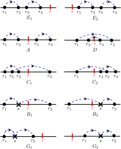
Figure 14: Two-loop diagrams for the quadratic order term $W_{2}$ in Eq. (96). The diagrams are categorized according to relative position of the loops with respect to $\tau$. For diagram $E_{1}$, the times $r_{1}<r_{2}<\tau$ and $r_{3}<r_{4}<\tau$, excluding cases where any two times are equal (contracted). Similar convention is adopted for the diagrams $E_{2}$, $A$, $D$, and $C$, where $r_{1}<r_{2}$, $r_{3}<r_{4}$, and their relative position with $\tau$ indicated in the diagrams. For diagrams $B$ and $G$ we consider, $r_{2}>s>r_{1}$ being on the same side of $\tau$ as indicated. A solid disk denotes a ‘charge’ $\dot{x}(r)$ for the associated point $r$, and a cross denotes a ‘charge’ $2D$. A dashed line indicates coupling between points $r_{i}$ and $r_{j}$ with a coupling strength $e^{y(r_{i}-r_{j})}$.

Considering the contribution of the diagrams in Figs. 12 and 13, resulting into Eq. (96), we see that the relevant contribution for $W_{2}$ comes from the 2-loop diagrams (a) and (c) in Fig. 12. Considering the relative position of the loops with respect to $\tau$, we write the amplitude $W_{2}$ as a sum of the following ten diagrams,

$$W_{2} =a+c$$ (117)

$$=\left(E_{1}+E_{2}\right)+A+D+\left(C_{1}+C_{2}\right)$$ (118)

$$\quad+\left(B_{1}+B_{2}\right)+\left(G_{1}+G_{2}\right).$$ (119)

This is shown in Fig. 14. Explicit formulas of their amplitudes are given in App. G. We shall see that among these diagrams, only diagram $D$ contributes to the non-trivial term $\mathcal{F}^{\rm last}$ in Eq. (47), whereas the remaining diagrams contribute to the power-law prefactor only.

Here, we present the double Laplace transformation Eq. (77) of the amplitude of these diagrams, for small $x_{0}$ limit. Their derivation is similar to those of the amplitude of zeroth and linear order terms in Eqs. (103, 109). We defer their explicit calculation to the App. G.

For small $x_{0}$, we get

$$\widetilde{D}(s\,\kappa,s)\simeq\frac{x_{0}}{Ds}\times\frac{\widetilde{\mathcal{D}}(1+\kappa)}{\sqrt{1+\kappa}}$$ (120)

with

$$\widetilde{\mathcal{D}}(z) =-2\int_{0}^{\Lambda/s}\frac{dy_{1}dy_{2}}{y_{1}^{2}y_{2}^{2}}\sqrt{z}\sqrt{1+y_{1}+y_{2}}$$ (121)

$$\quad\times\left(\sqrt{1+y_{1}+y_{2}}-\sqrt{1+y_{1}}-\sqrt{1+y_{2}}+1\right)$$ (122)

$$\quad\times\bigg{(}\sqrt{z+y_{1}+y_{2}}-\sqrt{z+y_{1}}-\sqrt{z+y_{2}}+\sqrt{z}\bigg{)}.$$

The amplitude of the diagrams $B$ and $C$ is of order $x_{0}^{2}$ for small $x_{0}$,

$$\widetilde{B}(s\,\kappa,s)\simeq\widetilde{C}(s\,\kappa,s)\sim x_{0}^{2}.$$ (123)

This can be seen from the argument given in the remark below Eq. (109). Their explicit derivation is in Appendix G.2.4.

The amplitude for the remaining diagrams is of order $x_{0}$, and given as follows. For small $x_{0}$,

$$\widetilde{E}_{1}(s\,\kappa,s)+\widetilde{E}_{2}(s\,\kappa,s) \simeq\frac{x_{0}}{s}\times\frac{\widetilde{\mathcal{E}}(1+\kappa)+\widetilde{\mathcal{E}}(1)}{D\sqrt{1+\kappa}},$$ (124)

where

$$\widetilde{\mathcal{E}}(z)=-\frac{1}{2}\int_{0}^{\Lambda/s}\frac{dy_{1}dy_{2}}{y_{1}^{2}y_{2}^{2}}\bigg{\{}(z+y_{1})(z+y_{2})\qquad$$

$$+\sqrt{z}\,\big{(}\sqrt{z}-\sqrt{z+y_{1}}-\sqrt{z+y_{2}}\big{)}\bigg{[}\sqrt{z+y_{1}}$$

$$\times\big{(}\sqrt{z}-\sqrt{z+y_{1}}\big{)}+\sqrt{z+y_{2}}\left(\sqrt{z}-\sqrt{z+y_{2}}\right)$$

$$+\big{(}\sqrt{z}-\sqrt{z+y_{1}}-\sqrt{z+y_{2}}\big{)}^{2}-$$ (125)

$$2\bigg{(} \sqrt{z+y_{1}+y_{2}}-\sqrt{z+y_{1}}-\sqrt{z+y_{2}}+\sqrt{z}\bigg{)}^{2}\bigg{]}\bigg{\}}.\qquad$$ (126)

Similarly, for small $x_{0}$,

$$\widetilde{A}(s\,\kappa,s)\simeq-\frac{x_{0}}{s}\times\frac{\widetilde{\mathcal{A}}(1+\kappa)\widetilde{\mathcal{A}}(1)}{D\sqrt{1+\kappa}}$$ (127)

with Eq. (108), and

$$\widetilde{G}_{1}(s\,\kappa,s)+\widetilde{G}_{2}(s\,\kappa,s)\simeq\frac{x_{0}}{s}\times\frac{\widetilde{\mathcal{G}}(1+\kappa)+\widetilde{\mathcal{G}}(1)}{D\sqrt{1+\kappa}},$$ (128)

where

$$\widetilde{\mathcal{G}}(z)= \int_{0}^{\Lambda/s}\frac{dy_{1}dy_{2}}{y_{1}^{2}y_{2}^{2}}$$ (129)

$$\times\left[\frac{(\sqrt{z+y_{2}}-\sqrt{z})^{2}y_{1}^{2}-(\sqrt{z+y_{1}}-\sqrt{z})^{2}y_{2}^{2}}{(y_{1}-y_{2})}\right].$$

Considering the amplitude of these 2-loop diagrams in Eq. (119) we get the double Laplace transform Eq. (77) of $W_{2}(\tau,T)$ in Eq. (96). For small $x_{0}$ it reads

$$\widetilde{W}_{2} (s\,\kappa,s)\simeq\frac{x_{0}}{s\,D\sqrt{1+\kappa}}\bigg{[}\widetilde{\mathcal{E}}(1+\kappa)+\widetilde{\mathcal{E}}(1)-$$ (130)

$$\widetilde{\mathcal{A}}(1+\kappa)\widetilde{\mathcal{A}}(1)+\widetilde{\mathcal{D}}(1+\kappa)+\widetilde{\mathcal{G}}(1+\kappa)+\widetilde{\mathcal{G}}(1)\bigg{]}.\quad$$ (131)

VI.4 Result for $\mathcal{F}^{\rm last}(\kappa,H)$

From the results in Eqs. (103), (109), and (131) we obtain the double Laplace transform Eq. (77) of $W(\tau,T)$ in Eq. (93) in an exponential form,

$$\widetilde{W}(s\,\kappa,s)=\mathscr{D}_{\begin{subarray}{c}\tau\to s\,\kappa\\ T\to s\end{subarray}}\odot W(\tau,T)\simeq\frac{x_{0}}{s}\times\frac{e^{\widetilde{\mathcal{W}}(\kappa)}}{\sqrt{1+\kappa}},$$ (132)

Here $x_{0}$ is small, and we used $D$ in Eq. (14) to explicitly write the exponential term $\widetilde{\mathcal{W}}=\varepsilon\widetilde{\mathcal{W}}_{1}+\varepsilon^{2}\widetilde{\mathcal{W}}_{2}+\cdots$, with

$$\widetilde{\mathcal{W}}_{1}(\kappa)= \;\widetilde{\mathcal{A}}(1)-\widetilde{\mathcal{A}}(1+\kappa)+2(\ln\Lambda+\gamma_{\rm E}-1),$$ (133a)

$$\widetilde{\mathcal{W}}_{2}(\kappa)= \;\widetilde{\mathcal{E}}(1+\kappa)+\widetilde{\mathcal{E}}(1)+\widetilde{\mathcal{D}}(1+\kappa)$$ (133b)

$$-\widetilde{\mathcal{A}}(1+\kappa)\widetilde{\mathcal{A}}(1)+\widetilde{\mathcal{G}}(1+\kappa)+\widetilde{\mathcal{G}}(1)$$ (133c)

$$-\frac{1}{2}\left[\widetilde{\mathcal{A}}(1)-\widetilde{\mathcal{A}}(1+\kappa)\right]^{2}+2\left[1-\frac{\pi^{2}}{6}\right].\qquad\qquad$$ (133d)

To relate to the exponential form in Eq. (83) we note that the Laplace transform of $N_{T}$ in Eq. (90) is

$$\widetilde{N}(s)=\widetilde{W}(0,s).$$ (134)

The simple $s$-dependence in Eq. (132) (for $\Lambda\to\infty$) makes it easy to invert the Laplace transform, giving

$$N(T)\simeq x_{0}\;e^{\widetilde{\mathcal{W}}(0)}\qquad\text{for small {\hbox{x_0}}.}$$ (135)

This means, for small $x_{0}$, $N(T)\equiv N$ is independent of $T$, and the double Laplace transform of $P_{T}(\tau)$ in Eq. (89) is

$$\widetilde{P}(\lambda,s)\simeq\frac{\widetilde{W}(\lambda,s)}{N}\qquad\text{for small {\hbox{x_0}}.}$$ (136)

Then, using Eq. (132) and comparing with Eqs. (79) and (83) gives

$$\widetilde{\mathcal{F}}^{\rm last}(\kappa,H)=\widetilde{\mathcal{W}}(\kappa)-\widetilde{\mathcal{W}}(0),$$ (137)

which we shall need to determine $\mathcal{F}(\vartheta,H)$ in Eq. (84). The leading terms in its perturbation expansion Eq. (86a) is given by

$$\widetilde{\mathcal{F}}_{1}^{\rm last}(\kappa)= \;\widetilde{\mathcal{A}}(1)-\widetilde{\mathcal{A}}(1{+}\kappa),$$ (138a)

$$\widetilde{\mathcal{F}}_{2}^{\rm last}(\kappa)= \;\left[\widetilde{\mathcal{D}}(1{+}\kappa)-\widetilde{\mathcal{D}}(1)\right]+\bigg{[}\widetilde{\mathcal{E}}(1{+}\kappa)+\widetilde{\mathcal{G}}(1{+}\kappa)$$ (138b)

$$-\frac{1}{2}\widetilde{\mathcal{A}}^{2}(1{+}\kappa)-\left(\widetilde{\mathcal{E}}(1)+\widetilde{\mathcal{G}}(1)-\frac{1}{2}\widetilde{\mathcal{A}}^{2}(1)\right)\bigg{]}.$$ (138c)

We have numerically verified that, for $\Lambda\to\infty$,

$$\widetilde{\mathcal{E}}(z)+\widetilde{\mathcal{G}}(z)-\frac{1}{2}\widetilde{\mathcal{A}}^{2}(z)=\left(1+\ln(2)\right)^{2}-\frac{5\pi^{2}}{12}.$$ (139)

Therefore, the only non-vanishing contribution for $\Lambda\to\infty$ comes from the diagram $D$, leading to

$$\widetilde{\mathcal{F}}_{2}^{\rm last}(\kappa) = \widetilde{\mathcal{D}}(1{+}\kappa)-\widetilde{\mathcal{D}}(1).$$ (140)

• We see that Eq. (137) is consistent with the condition Eq. (88). Moreover, we shall see that the integrals in Eq. (138a) and Eq. (140) converge in the $\Lambda\to\infty$ limit, as one would expect for our theory to be correct.

• Note that in Eq. (133) the contribution from diffusion constant $D$ in Eq. (14) is constant, which cancels in Eq. (137). This is expected as the distribution of $t_{\rm last}$ is independent of the diffusion constant, whereas as a distribution involving space would depend on $D$. The same applies for the distribution of $t_{\rm max}$ and $t_{\rm pos}$.

For the leading-order term Eq. (138a), explicitly carrying out the integral in Eq. (108) in the limit of $\Lambda\to\infty$, we get

$$\widetilde{\mathcal{F}}_{1}^{\rm last}(\kappa)=\ln(1+\kappa),$$ (141)

whose $\mathcal{K}^{-1}$-transformation is (see Eq. (283))

$$\mathcal{K}^{-1}_{\kappa\to\vartheta}\odot\widetilde{\mathcal{F}}_{1}^{\rm last}(\kappa)=-\ln\tfrac{\vartheta}{(1-\vartheta)}=-\mathcal{R}^{\rm last}(\vartheta).$$ (142)

Using the result Eq. (86b) for $t_{\rm last}$ gives the leading-order result in Eq. (51a).

For the second-order term in Eq. (86d) we use Eq. (140), Eq. (51a), and

$$\mathcal{K}^{-1}_{\kappa\to\vartheta}\odot\widetilde{\mathcal{F}}_{1}^{\rm last}(\kappa)^{2}=\mathcal{R}^{\rm last}(\vartheta)^{2}-\pi^{2}$$ (143)

(using the identity Eq. (284)) to write

$$\mathcal{F}_{2}^{\rm last} (\vartheta)=\mathcal{K}_{\kappa\rightarrow\vartheta}^{-1}\odot\left[\widetilde{\mathcal{D}}(1+\kappa)-\widetilde{\mathcal{D}}(1)\right]-\frac{\pi^{2}}{2},$$ (144)

where we use linearity of the operator $\mathcal{K}^{-1}$.

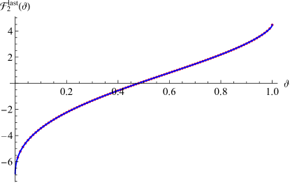
Figure 15: The dotted points (colored red) show results of numerical integration for $\mathcal{F}_{2}^{\rm last}(\vartheta)$ in Eq. (52). The solid line is the polynomial fit in Eq. (55), which gives a good estimation for $\mathcal{F}_{2}^{\rm last}(\vartheta)$.

The integral for $\widetilde{\mathcal{D}}(z)$ in Eq. (121) is convergent in the limit of $\Lambda\to\infty$, but it is hard to evaluate analytically. The expression for $\mathcal{F}_{2}^{\rm last}(\vartheta)$ in Eq. (52) is obtained [76] by exchanging the order of $\mathcal{K}_{\kappa\rightarrow\vartheta}^{-1}$ transformation and the $y$-integrals in Eqs. (144) and (121). (For several other examples like in Eqs. (138a) and (142) where integration can be explicitly carried out, we have verified that this exchange of order gives the correct result.) The resulting function $\mathcal{F}_{2}^{\rm last}(\vartheta)$ in Eq. (52) is plotted in Fig. 15 along with a polynomial estimation given in Eq. (55). The expression Eq. (52) is in good agreement with our computer simulation result in Fig. 7.

VII Distribution of the time $t_{\rm max}$ when the fBm attains maximum

The probability for an fBm, starting at $X_{0}=0$ and evolving till time $T$, to attain its maximum at time $t_{\rm max}=\tau$ can be expressed as

$$P_{T}(t_{\rm max}=\tau)=\frac{W(\tau,T)}{N(T)}.$$ (145)

Here $W(\tau,T)$ is the weight of all contributing trajectories, and $N(T)$ is the corresponding normalization. We use the same notations as in Sec. VI. Note, however, that the definition of these quantities ($W$, $N$, etc.) is specific to the problem in this section.

Noting the symmetry of the problem (illustrated in Fig. 16), we write

$$W(\tau,T)=\, \int_{0}^{\infty}dm_{1}\int_{0}^{\infty}dm_{2}\int_{x(0)=m_{1}}^{x(T)=m_{2}}\mathcal{D}[x]$$ (146)

$$\qquad\times\delta(x(\tau)-x_{0})\prod_{t=0}^{T}\Theta[x(t)]e^{-S[x]}.\qquad$$ (147)

The probability density $P_{T}(\tau)$ in Eq. (145) is obtained by taking the limit of $x_{0}\to 0$. (Like in the previous section, we do not write any explicit reference to $x_{0}$, unless necessary.)

Figure 16: The dark solid curve is a schematic of paths $X_{t}$ for Eq. (146), where the stripped line indicates an absorbing boundary at the origin. For $x_{0}\to 0$, there is an one-to-one correspondence with an fBm path (indicated by gray dashed curve) that contributes for the process to attain its maximum $m_{1}$ at time $t_{\rm max}$.

The perturbation expansion Eq. (7) of the fBm action $S$ leads to an expansion of $W$ similar to Eq. (93) with

$$W_{0}(\tau,T) =\int_{0}^{\infty}dm_{1}\int_{0}^{\infty}dm_{2}\;\mathopen{\hbox{${\langle}$}\kern-2.72221pt\leavevmode\hbox{${\langle}$}}1\mathclose{\hbox{${\rangle}$}\kern-2.72221pt\leavevmode\hbox{${\rangle}$}}_{(m_{1},m_{2})},$$ (148)

$$W_{1}(\tau,T) =\int_{0}^{\infty}dm_{1}\int_{0}^{\infty}dm_{2}\;\mathopen{\hbox{${\Big{\langle}}$}\kern-2.72221pt\leavevmode\hbox{${\Big{\langle}}$}}\frac{S_{1}}{2D}\mathclose{\hbox{${\Big{\rangle}}$}\kern-2.72221pt\leavevmode\hbox{${\Big{\rangle}}$}}_{(m_{1},m_{2})},$$ (149)

$$W_{2}(\tau,T) =\int_{0}^{\infty}dm_{1}\int_{0}^{\infty}dm_{2}\;\mathopen{\hbox{${\bigg{\langle}}$}\kern-2.72221pt\leavevmode\hbox{${\bigg{\langle}}$}}\frac{S_{1}^{2}}{8D^{2}}-\frac{S_{2}}{D}\mathclose{\hbox{${\bigg{\rangle}}$}\kern-2.72221pt\leavevmode\hbox{${\bigg{\rangle}}$}}_{(m_{1},m_{2})}.$$ (150)

By the double-angular brackets we denote

$$\mathopen{\hbox{${\langle}$}\kern-2.72221pt\leavevmode\hbox{${\langle}$}}O[x]\mathclose{\hbox{${\rangle}$}\kern-2.72221pt\leavevmode\hbox{${\rangle}$}}_{(m_{1},m_{2})}$$ (151)

$$:=\int\limits_{x(0)=m_{1}}^{x(T)=m_{2}}\mathcal{D}[x]\delta\big{(}x(\tau)-x_{0}\big{)}\prod_{t=0}^{T}\Theta[x(t)]\,e^{-\frac{S_{0}}{D}}O[x(t)].$$

Here, both $m_{1}\geq 0$ and $m_{2}\geq 0$, and the average is over trajectories sketched in Fig. 16 with the standard Brownian measure. Note that this definition is different from the one in Eq. (97), due to the different boundary conditions employed there. We will now in turn study averages at different orders, expressed in terms of the Brownian propagator Eq. (98) in presence of an absorbing wall. This is similar to the analysis of $t_{\rm last}$ in the previous Sec. VI.

VII.1 Zeroth order

Similar to Eq. (101), we write the double Laplace transformation of Eq. (148) as

$$\widetilde{W}_{0}(\lambda,s)=\int_{0}^{\infty}dm_{1}\int_{0}^{\infty}dm_{2}\,\widetilde{Z}^{+}_{s+\lambda}(m_{1},x_{0})\,\widetilde{Z}^{+}_{s}(x_{0},m_{2}).$$

Using Eq. (102) and integrating, it is easy to see that for small $x_{0}$,

$$\widetilde{W}_{0}(s\,\kappa,s)\simeq\frac{x_{0}^{2}}{Ds}\times\frac{1}{\sqrt{1+\kappa}}.$$ (152)

The leading non-vanishing term is of order $x_{0}^{2}$, and its amplitude is same as in Eq. (103). This gives the well-known arcsine-law (4) for $t_{\rm max}$.

VII.2 Linear order: 1-loop diagrams

Similar to Eq. (106a) we write $W_{1}$ in Eq. (149) in three parts according to the order of $(r_{1},r_{2},\tau)$. Their diagrammatic representation is similar to the 1-loop diagrams in Fig. 11, but their amplitude is different. They are given by

$$A_{1}(\tau,T)=\frac{1}{2D} \int_{0}^{\infty}dm_{1}dm_{2}\int_{0}^{\Lambda}dy$$

$$\times J_{\tau}^{+}(m_{1},x_{0};-y,y)Z_{T-\tau}^{+}(x_{0},m_{2}),$$ (153a)

$$A_{2}(\tau,T)=\frac{1}{2D} \int_{0}^{\infty}dm_{1}dm_{2}\int_{0}^{\Lambda}dy$$

$$\times Z_{\tau}^{+}(m_{1},x_{0})J_{T-\tau}^{+}(x_{0},m_{2};-y,y),$$ (153b)

$$A_{3}(\tau,T)=\frac{1}{2D} \int_{0}^{\infty}dm_{1}dm_{2}\int_{0}^{\Lambda}dy$$

$$\times J_{\tau}^{+}(m_{1} ,x_{0};-y)J_{T{-}\tau}^{+}(x_{0},m_{2};y)\;e^{-y\tau}.~{}~{}~{}$$ (153c)

The function $$J_{t}^{+}$$ is the counterpart of Eq. (107) in presence of an absorbing wall at the origin.

Their double Laplace transform Eq. (77) gives

$$\widetilde{A}_{1}(\lambda,s)=\frac{1}{2D} \int_{0}^{\infty}dm_{1}dm_{2}\int_{0}^{\Lambda}dy$$

$$\times \widetilde{J}_{s+\lambda}^{+}(m_{1},x_{0};-y,y)\widetilde{Z}_{s}^{+}(x_{0},m_{2}),$$ (154a)

$$\widetilde{A}_{2}(\lambda,s)=\frac{1}{2D} \int_{0}^{\infty}dm_{1}dm_{2}\int_{0}^{\Lambda}dy$$

$$\times \widetilde{Z}_{s+\lambda}^{+}(m_{1},x_{0})\widetilde{J}_{s}^{+}(x_{0},m_{2};-y,y),$$ (154b)

$$\widetilde{A}_{3}(\lambda,s)=\frac{1}{2D} \int_{0}^{\infty}dm_{1}dm_{2}\int_{0}^{\Lambda}dy$$

$$\times \widetilde{J}_{s+\lambda+y}^{+}(m_{1},x_{0};-y)\widetilde{J}_{s}^{+}(x_{0},m_{2};y).$$ (154c)

These integrals can be evaluated explicitly using the results in Apps. L and N, specifically Eqs. (300), (430), and their symmetry properties for evaluating Eqs. (154a), (154b), as well as Eqs. (462) and (464) for evaluating Eq. (154c). For small $x_{0}$, we get

$$\widetilde{A}_{1}(s\,\kappa,s) \simeq\frac{x_{0}^{2}}{Ds}\times\frac{\widetilde{\mathcal{A}}(1+\kappa)}{\sqrt{1+\kappa}},$$ (155)

$$\widetilde{A}_{2}(s\,\kappa,s) \simeq\frac{x_{0}^{2}}{Ds}\times\frac{\widetilde{\mathcal{A}}(1)}{\sqrt{1+\kappa}},$$ (156)

$$\widetilde{A}_{3}(s\,\kappa,s) \simeq\frac{x_{0}^{2}}{Ds}\times\frac{\widetilde{{\mathcal{A}_{3}}}(1+\kappa)}{\sqrt{1+\kappa}},$$ (157)

with $\widetilde{\mathcal{A}}(z)$ defined in Eq. (108) and

$$\widetilde{{\mathcal{A}_{3}}}(z)=-2\int_{0}^{\Lambda/s}\frac{dy}{y^{2}}\Big{(}\sqrt{z+y}-\sqrt{z}\Big{)}\Big{(}\sqrt{1+y}-1\Big{)}.$$ (158)

Summing all three contributions we get the double Laplace transform Eq. (77) of the linear-order term $W_{1}(\tau,T)$ in Eq. (149). It reads, for small $x_{0}$,

$$\widetilde{W}_{1}(s\,\kappa,s)\simeq\frac{x_{0}^{2}}{sD}\times\frac{\widetilde{\mathcal{A}}(1+\kappa)+\widetilde{\mathcal{A}}(1)+\widetilde{{\mathcal{A}_{3}}}(1+\kappa)}{\sqrt{1+\kappa}}.$$ (159)

We note the simplification

$$\widetilde{\mathcal{A}} (z)+\widetilde{\mathcal{A}}(1)+\widetilde{{\mathcal{A}_{3}}}(z)$$ (160)

$$=\int_{0}^{\Lambda/s}\!\!\frac{dy}{y^{2}}\left[\left(\sqrt{z+y}-\sqrt{z}\right)-\left(\sqrt{1+y}-1\right)\right]^{2}.\qquad$$ (161)

VII.3 Quadratic order

Similar to Eq. (119), we find that the second-order term $W_{2}$ in Eq. (150) is composed of the 2-loop diagrams in Fig. 14. The amplitudes of these diagrams are different for this problem. Here we summarize their result for small $x_{0}$. Their derivation is given in App. H.

The list below contains the double Laplace transform of all 2-loop diagrams. All amplitudes are of order $x_{0}^{2}$ for small $x_{0}$. Note that many diagrams are the same as in the problem of $t_{\rm last}$ in Sec. VI; this may not be surprising as the same power-law corrections for $\vartheta\to 0$ and $\vartheta\to 1$ are also present in the distribution of $t_{\rm last}$.

The list of already calculated diagrams reads ($x_{0}\ll 1$):

$$\widetilde{E}_{1}(s\,\kappa,s)+\widetilde{E}_{2}(s\,\kappa,s) \simeq\frac{x_{0}^{2}}{sD}\times\frac{\widetilde{\mathcal{E}}(1+\kappa)+\widetilde{\mathcal{E}}(1)}{\sqrt{1+\kappa}},$$ (162)

with $\widetilde{\mathcal{E}}$ given in Eq. (126).

$$\widetilde{A}(s\,\kappa,s)\simeq\frac{x_{0}^{2}}{sD}\times\frac{\widetilde{\mathcal{A}}(1+\kappa)\widetilde{\mathcal{A}}(1)}{\sqrt{1+\kappa}},$$ (163)

with $\widetilde{\mathcal{A}}(z)$ given in Eq. (108).

$$\widetilde{G}_{1}(s\,\kappa,s)+\widetilde{G}_{2}(s\,\kappa,s)\simeq\frac{x_{0}^{2}}{sD}\times\frac{\widetilde{\mathcal{G}}(1+\kappa)+\widetilde{\mathcal{G}}(1)}{\sqrt{1+\kappa}},$$ (164)

with $\widetilde{\mathcal{G}}(z)$ given in Eq. (129).

The amplitudes of the remaining diagrams are different. We get, for small $x_{0}$,

$$\widetilde{D}(s\,\kappa,s)=\frac{x_{0}^{2}}{sD}\times\frac{\widetilde{\mathcal{D}}(1+\kappa)}{\sqrt{1+\kappa}},$$ (165)

with

$$\widetilde{\mathcal{D}}(z) =2\int_{0}^{\Lambda/s}\frac{dy_{1}dy_{2}}{y_{1}^{2}y_{2}^{2}}\sqrt{z+y_{1}+y_{2}}\,\sqrt{1+y_{1}+y_{2}}$$ (166)

$$\quad\times\left(\sqrt{1+y_{1}+y_{2}}-\sqrt{1+y_{1}}-\sqrt{1+y_{2}}+1\right)$$ (167)

$$\quad\times\bigg{(}\sqrt{z+y_{1}+y_{2}}-\sqrt{z+y_{1}}-\sqrt{z+y_{2}}+\sqrt{z}\bigg{)}.$$ (168)

The difference to Eq. (121) is in the first term inside the integrals and the overall sign.

The leading non-vanishing amplitudes of diagrams $B$ and $C$ are of order $x_{0}^{2}$, and unlike in Sec. VI, these diagrams are relevant here. Their Laplace transform, for small $x_{0}$ are

$$\widetilde{B}_{1}(s\,\kappa,s)+\widetilde{B}_{2}(s\,\kappa,s)\simeq\frac{x_{0}^{2}}{s}\times\frac{\widetilde{\mathcal{B}}(1+\kappa)}{D\sqrt{1+\kappa}},$$ (169)

where

$$\widetilde{\mathcal{B}}(z)=2\int\limits_{0}^{\Lambda/s}\!\!\frac{dy_{1}dy_{2}}{y_{1}^{2}y_{2}^{2}(y_{1}-y_{2})}\;\bigg{[}y_{2}^{2}(\sqrt{z{+}y_{1}}{-}\sqrt{z})(\sqrt{1{+}y_{1}}{-}1)$$ (170)

$$\qquad\qquad\qquad-y_{1}^{2}(\sqrt{z+y_{2}}-\sqrt{z})(\sqrt{1+y_{2}}-1)\bigg{]}$$ (171)

and

$$\widetilde{C}_{1}(s\,\kappa,s)+\widetilde{C}_{2}(s\,\kappa,s)\simeq\frac{x_{0}^{2}}{s}\times\frac{\left(\widetilde{\mathcal{C}}(1,\,1+\kappa)+\widetilde{\mathcal{C}}(1+\kappa,\,1)\right)}{D\sqrt{1+\kappa}},$$ (172)

where

$$\widetilde{\mathcal{C}} (z_{1},z_{2})=2\int_{0}^{\Lambda/s}\frac{dy_{1}dy_{2}}{\;y_{1}^{2}\;y_{2}^{2}}\left(\sqrt{z_{1}}-\sqrt{z_{1}+y_{1}}\right)\sqrt{z_{2}+y_{1}}$$

$$~{}~{}~{}~{}~{}\times\left(\sqrt{z_{2}+y_{1}+y_{2}}-\sqrt{z_{2}+y_{1}}-\sqrt{z_{2}+y_{2}}+\sqrt{z_{2}}\right)^{2}.$$ (173)

From the amplitude of all 2-loop diagrams in Eq. (119) we get the double Laplace transform of $W_{2}(\tau,T)$ in Eq. (150), for small $x_{0}$,

$$\widetilde{W}_{2}(s\,\kappa,s)\simeq\frac{x_{0}^{2}}{s\,D\sqrt{1+\kappa}}\bigg{[}\widetilde{\mathcal{E}}(1+\kappa)+\widetilde{\mathcal{E}}(1)+$$

$$\widetilde{\mathcal{A}}(1+\kappa)\widetilde{\mathcal{A}}(1)+\widetilde{\mathcal{D}}(1+\kappa)+\widetilde{\mathcal{C}}(1,\,1+\kappa)+\widetilde{\mathcal{C}}(1+\kappa,\,1)$$

$$\qquad\qquad+\widetilde{\mathcal{B}}(1+\kappa)+\widetilde{\mathcal{G}}(1+\kappa)+\widetilde{\mathcal{G}}(1)\bigg{]}.$$ (174)

VII.4 Result for $\mathcal{F}^{\rm max}(\kappa,H)$

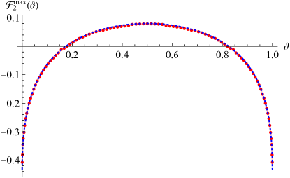
Figure 17: The dotted points (colored red) show $\mathcal{F}_{2}^{\rm max}(\vartheta)$ evaluated by numerical integration from Eq. (190). The solid line is the polynomial in Eq. (57), which gives a good estimation for $\mathcal{F}_{2}^{\rm max}(\vartheta)$.

Taking the results in Eqs. (152), (159), (174), and the expansion (14) we write in an exponential form analogous to Eq. (132), where, for this problem,

$$\widetilde{\mathcal{W}}_{1}(\kappa)= \widetilde{\mathcal{A}}(1+\kappa)+\widetilde{\mathcal{A}}(1)+\widetilde{{\mathcal{A}_{3}}}(1+\kappa)+2(\ln\Lambda+\gamma_{\rm E}-1),$$

$$\widetilde{\mathcal{W}}_{2}(\kappa)= \Big{[}\widetilde{\mathcal{E}}(1+\kappa)+\widetilde{\mathcal{E}}(1)+\widetilde{\mathcal{A}}(1+\kappa)\widetilde{\mathcal{A}}(1)+\widetilde{\mathcal{D}}(1+\kappa)$$

$$+\widetilde{\mathcal{C}}(1,\,1+\kappa)+\widetilde{\mathcal{C}}(1+\kappa,\,1)+\widetilde{\mathcal{B}}(1+\kappa)$$

$$+\widetilde{\mathcal{G}}(1+\kappa)+\widetilde{\mathcal{G}}(1)\Big{]}-\frac{1}{2}\Big{[}\widetilde{\mathcal{A}}(1+\kappa)+\widetilde{\mathcal{A}}(1)$$

$$+\widetilde{{\mathcal{A}_{3}}}(1+\kappa)\Big{]}^{2}+2\left(1-\frac{\pi^{2}}{6}\right).$$

The rest of the analysis is very similar to that in Sec. VI.4. To leading order we get

$$\widetilde{\mathcal{F}}_{1}^{\rm max}(\kappa)=\widetilde{\mathcal{W}}_{1}(\kappa)-\widetilde{\mathcal{W}}_{1}(0)$$ (175)

$$=\int_{0}^{\Lambda/s}\frac{dy}{y^{2}}\left(\sqrt{1+\kappa+y}-\sqrt{1+\kappa}-\sqrt{1+y}+1\right)^{\!2}.\qquad$$

Explicitly carrying out the integral in the $\Lambda\to\infty$ limit yields

$$\widetilde{\mathcal{F}}_{1}^{\rm max} (\kappa)=-8\ln 2-\left(1+\sqrt{1+\kappa}\right)\ln(1+\kappa)$$ (176)

$$+\frac{2}{\sqrt{1+\kappa}}\left(1+\sqrt{1+\kappa}\right)^{2}\ln\left(1+\sqrt{1+\kappa}\right).~{}~{}~{}~{}~{}~{}~{}~{}$$ (177)

Its inverse transform Eq. (85) is (see Eq. (287))

$$\mathcal{K}_{\kappa\rightarrow\vartheta}^{-1}\odot\widetilde{\mathcal{F}}_{1}^{\rm max}(\kappa) = -8\ln 2+\psi\left(\sqrt{\frac{\vartheta}{1-\vartheta}}\right)$$ (178)

$$-\ln(\vartheta(1-\vartheta)),$$

with $\psi(x)$ defined in Eq. (51c). Then Eq. (86b) with $\mathcal{R}^{\rm max}(\vartheta)=\ln(\vartheta(1-\vartheta))$ gives the leading-order term

$$\mathcal{F}^{\rm max}_{1}(\vartheta)=-8\ln 2+\psi\left(\sqrt{\frac{\vartheta}{1-\vartheta}}\right).$$ (179)

The expression in Eq. (179) differs from Eq. (51b) by a constant, which comes from our convention that for the latter the integral over $\vartheta$ vanishes.

At second order, we get

$$\widetilde{\mathcal{F}}_{2}^{\rm max}(\kappa) =\widetilde{\mathcal{W}}_{2}(\kappa)-\widetilde{\mathcal{W}}_{2}(0)$$

$$=\bigg{[}\widetilde{\mathcal{D}}(1 +\kappa)-\frac{1}{2}\widetilde{{\mathcal{A}_{3}}}(1+\kappa)^{2}-\left(\widetilde{\mathcal{D}}(1)-\frac{1}{2}\widetilde{{\mathcal{A}_{3}}}(1)^{2}\right)\bigg{]}$$

$$+\bigg{[}\widetilde{\mathcal{B}} (1+\kappa)+\widetilde{\mathcal{C}}(1,\,1+\kappa)+\widetilde{\mathcal{C}}(1+\kappa,\,1)$$ (180)

$$\qquad\quad-\widetilde{{\mathcal{A}_{3}}}(1+\kappa)\left(\widetilde{\mathcal{A}}(1+\kappa)+\widetilde{\mathcal{A}}(1)\right)$$ (181)

$$-\left(\widetilde{\mathcal{B}}(1)+2\widetilde{\mathcal{C}}(1,\,1)-2\widetilde{{\mathcal{A}_{3}}}(1)\widetilde{\mathcal{A}}(1)\right)\bigg{]}$$ (182)

$$+\bigg{[}\widetilde{\mathcal{E}} (1+\kappa)+\widetilde{\mathcal{G}}(1+\kappa)-\frac{1}{2}\widetilde{\mathcal{A}}^{2}(1+\kappa)$$ (183)

$$\qquad\qquad-\left(\widetilde{\mathcal{E}}(1)+\widetilde{\mathcal{G}}(1)-\frac{1}{2}\widetilde{\mathcal{A}}^{2}(1)\right)\bigg{]}.$$ (184)

The terms are written such that each square bracket remains finite for $\Lambda\to\infty$ limit. In fact, we see that the expression in the last square bracket is same as in Eq. (138c) and it vanishes for $\Lambda\to\infty$. Rest two square brackets give $\widetilde{\mathcal{F}}_{2}^{\rm max}(\kappa)$ for the $\Lambda\to\infty$.

• We see that for $\kappa=0$, both $\widetilde{\mathcal{F}}_{1}^{\rm max}(\kappa)$ and $\widetilde{\mathcal{F}}_{2}^{\rm max}(\kappa)$ vanish, which is consistent with the condition (88).

From Eq. (86d) and using linearity of the transformation $\mathcal{K}_{\kappa\rightarrow\vartheta}^{-1}$ we write

$$\mathcal{F}_{2}^{\rm max} (\vartheta)=\mathcal{K}_{\kappa\rightarrow\vartheta}^{-1}\odot\widetilde{\mathcal{F}}_{2}^{\rm max}(\kappa)+$$ (185)

$$\frac{1}{2}\Big{\{} \mathcal{K}_{\kappa\rightarrow\vartheta}^{-1}\odot\widetilde{\mathcal{F}}_{1}^{\rm max}(\kappa)^{2}-\left[\mathcal{F}_{1}^{\rm max}(\vartheta)-\mathcal{R}^{\rm max}(\vartheta)\right]^{2}\Big{\}}.$$

Using an identity Eq. (289) we see that

$$\mathcal{K}_{\kappa\rightarrow\vartheta}^{-1} \odot\widetilde{\mathcal{F}}_{1}^{\rm max}(\kappa)^{2}=$$ (186)

$$\Big{[}\mathcal{F}_{1}^{\rm max}(\vartheta)-\mathcal{R}^{\rm max}(\vartheta)\Big{]}^{2}-\psi_{2}\left(\sqrt{\frac{\vartheta}{1-\vartheta}}\right)^{\!2},\qquad$$ (187)

where we define

$$\psi_{2}(x)= 2\arctan x+x\ln\left(1+\frac{1}{x^{2}}\right)$$ (188)

$$-\left[2\arctan\frac{1}{x}+\frac{1}{x}\ln\left(1+x^{2}\right)\right].$$ (189)

This leads to our result

$$\mathcal{F}_{2}^{\rm max} (\vartheta)=\mathcal{K}_{\kappa\rightarrow\vartheta}^{-1}\odot\widetilde{\mathcal{F}}_{2}^{\rm max}(\kappa)-\frac{1}{2}\psi_{2}\left(\sqrt{\frac{\vartheta}{1-\vartheta}}\right)^{2}.$$ (190)

(We note that the last term is symmetric in $\vartheta\to 1-\vartheta$.)

It is hard to analytically evaluate the integrals in Eq. (184). Similar to Eq. (144), we determine $\mathcal{F}_{2}^{\rm max}(\vartheta)$ by exchanging the order of $\mathcal{K}$-transformation and integration. This gives, up to an additive constant,

$${\cal F}^{\rm max}_{2}(\vartheta) =-\frac{1}{2}\psi_{2}\left(\sqrt{\frac{\vartheta}{1-\vartheta}}\right)^{2}$$

$$+ 2\int_{0}^{\infty}\frac{dy_{1}dy_{2}}{y_{1}^{2}y_{2}^{2}}\;\Psi^{\rm max}\left(y_{1},y_{2},\frac{1-\vartheta}{\vartheta}\right),$$ (191)

where $\Psi^{\rm max}(y_{1},y_{2},z)$ has a lengthy expression given in the Appendix I. The expression is also given in the supplemental Mathematica notebook [76] for numerical evaluation.

Our result for ${\cal F}^{\rm max}_{2}(\vartheta)$ in Eq. (190) is plotted in Fig. 17, which agrees well with our computer simulation result in Fig. 7. For this, we evaluated both the ${\mathcal{K}}^{-1}$-transformation and the $y$-integration numerically.

VIII Distribution of time $t_{\rm pos}$ where the process is positive

Figure 18: Schematic of an fBm trajectory leading to positive time $t_{\rm pos}$. Times spent on the positive side is indicated by double-sided arrow.

This analysis is more involved compared to the analysis for $t_{\rm last}$ and $t_{\rm max}$. The main reason is that the expressions at second order are very cumbersome, and a lot of ingeniosity is needed to reduce them to a manageable size.

Analogous to Eq. (145), the probability that an fBm, starting at $X_{0}=0$ and evolving until time $T$, spends time $t_{\rm pos}=\tau$ being positive ($X_{t}>0$), can be expressed as

$$P_{T}(t_{\rm pos}=\tau)=\frac{W(\tau,T)}{N(T)},$$ (192)

where $W(\tau,T)$ is the weight of all fBm trajectories contributing to the event and $N(T)$ its normalization. Formally,

$$W(\tau,T)=\int\limits_{-\infty}^{\infty}dm\int\limits_{x(0)=0}^{x(T)=m}\!\!\mathcal{D}[x]\,\delta\bigg{(}\!\tau{-}\!\int\limits_{0}^{T}dt\,\Theta\big{(}x(t)\big{)}\!\bigg{)}e^{-S[x]},$$ (193)

where $\Theta(x)$ is the Heaviside step function. A sketch of such a trajectory is given in Fig. 18. We follow the same notations as in sections VI and VII. The definition of the quantities $W$, $N$, etc., is modified to measure the positive time.

Using the perturbation expansion of the fBm action in Eq. (7) we write (93), with

$$W_{0}(\tau,T) =\int_{-\infty}^{\infty}dm\,\mathopen{\hbox{${\langle}$}\kern-2.72221pt\leavevmode\hbox{${\langle}$}}1\mathclose{\hbox{${\rangle}$}\kern-2.72221pt\leavevmode\hbox{${\rangle}$}}_{(0,m)},$$ (194a)

$$W_{1}(\tau,T) =\int_{-\infty}^{\infty}dm\,\mathopen{\hbox{${\Big{\langle}}$}\kern-2.72221pt\leavevmode\hbox{${\Big{\langle}}$}}\frac{S_{1}}{2D}\mathclose{\hbox{${\Big{\rangle}}$}\kern-2.72221pt\leavevmode\hbox{${\Big{\rangle}}$}}_{(0,m)},$$ (194b)

$$W_{2}(\tau,T) =\int_{-\infty}^{\infty}dm\,\mathopen{\hbox{${\bigg{\langle}}$}\kern-2.72221pt\leavevmode\hbox{${\bigg{\langle}}$}}\frac{S_{1}^{2}}{8D^{2}}-\frac{S_{2}}{D}\mathclose{\hbox{${\bigg{\rangle}}$}\kern-2.72221pt\leavevmode\hbox{${\bigg{\rangle}}$}}_{(0,m)},$$ (194c)

where the double-angular brackets denote

$$\mathopen{\hbox{${\langle}$}\kern-2.72221pt\leavevmode\hbox{${\langle}$}}O[x]\mathclose{\hbox{${\rangle}$}\kern-2.72221pt\leavevmode\hbox{${\rangle}$}}_{(m_{1},m_{2})}$$ (195)

$$\quad:=\int\limits_{x(0)=m_{1}}^{x(T)=m_{2}}\!\!\mathcal{D}[x]\,\delta\bigg{(}\!\tau{-}\!\int\limits_{0}^{T}dt\,\Theta\big{(}x(t)\big{)}\!\bigg{)}e^{-\frac{S_{0}}{D}}O[x(t)].$$

This is an average over trajectories with Brownian measure.

VIII.1 Conditional propagator

In Sec. VI and Sec. VII, the amplitudes in the expansion (93) are expressed in terms of the free Brownian propagator $Z$ in Eq. (25) and its analogue $Z^{+}$ in presence of an absorbing wall. For amplitudes (194), it is natural to express in terms of a conditional Brownian propagator, defined by

$$\mathbb{Z}_{T}(m_{1},m_{2}|\tau)=\int\limits_{x(0)=m_{1}}^{x(T)=m_{2}}\!\!\mathcal{D}[x]\,\delta\bigg{(}\!\tau{-}\!\int\limits_{0}^{T}dt\,\Theta\big{(}x(t)\big{)}\!\bigg{)}e^{-\frac{S_{0}}{D}}.$$ (196)

This gives the weight of all Brownian paths starting at $m_{1}$ and ending at $m_{2}$ at time $T$ conditioned to spending time $\tau$ on the positive half.

Figure 19: Different Brownian paths for the conditional propagator in Eq. (197). ($\mathbb{A}$) Includes paths which have never crossed the origin, ($\mathbb{B}$) includes paths which have crossed the origin at least once.

To find an explicit expression for the conditional propagator, we write the associated paths into two groups,

$$\mathbb{Z}_{T}(m_{1},m_{2}|\tau)=\mathbb{A}_{T}(m_{1},m_{2}|\tau)+\mathbb{B}_{T}(m_{1},m_{2}|\tau),$$ (197)

shown in the Fig. 19. The term $\mathbb{A}$ is non-zero only for $\tau=0$ or $T$. Using Eq. (98), we write

$$\mathbb{A}_{T}(m_{1},m_{2}|\tau)= \Theta(m_{1})\Theta(m_{2})\delta(\tau-T)Z_{T}^{+}(m_{1},m_{2})$$

$$+\Theta( -m_{1})\Theta(-m_{2})\delta(\tau)Z_{T}^{+}(-m_{1},-m_{2}).$$

Its double Laplace transform can be written with the help of identity (104) as

$$\widetilde{\mathbb{A}}_{s}(m_{1},m_{2}|\lambda) = \Theta(m_{1})\Theta(m_{2})\widetilde{Z}_{s+\lambda}^{+}(m_{1},m_{2})$$

$$+ \Theta(-m_{1})\Theta(-m_{2})\widetilde{Z}_{s}^{+}(-m_{1},-m_{2}),$$

where expression (102) leads to

$$\widetilde{\mathbb{A}}_{s} (m_{1},m_{2}|\lambda)=\frac{\Theta(m_{1}m_{2})}{2\sqrt{D(s+\lambda\Theta(m_{1}))}}$$ (199)

$$\times\left[e^{-|m_{1}-m_{2}|\sqrt{\frac{s+\lambda\Theta(m_{1})}{D}}}-e^{-|m_{1}+m_{2}|\sqrt{\frac{s+\lambda\Theta(m_{1})}{D}}}\right].\qquad$$

The second part of Eq. (197) is defined by (see Fig. 19)

$$\mathbb{B}_{T}(m_{1},m_{2}|\tau)= \int\limits_{0}^{T}dt_{1}\int\limits_{t_{1}}^{T}dt_{2}\mathopen{\hbox{${\langle}$}\kern-2.72221pt\leavevmode\hbox{${\langle}$}}\delta\left(x(t_{1})\right)\delta\left(x(t_{2})\right)\mathclose{\hbox{${\rangle}$}\kern-2.72221pt\leavevmode\hbox{${\rangle}$}}_{(m_{1},m_{2})}$$ (200)

with $\tau$ specified in the average (195). One can estimate, for example, for $m_{1}>0$ and $m_{2}>0$,

$$\mathopen{\hbox{${\langle}$}\kern-2.72221pt\leavevmode\hbox{${\langle}$}}\delta\left(x(t_{1})\right)\delta\left(x(t_{2})\right)\mathclose{\hbox{${\rangle}$}\kern-2.72221pt\leavevmode\hbox{${\rangle}$}}_{(m_{1},m_{2})}= \mathcal{N}\;D^{2}\;\left[\lim_{x_{0}\to 0}\frac{Z^{+}_{t_{1}}(m_{1},x_{0})}{x_{0}}\right]$$

$$\times\mathscr{G}(\tau-t_{1}-t_{2},T-t_{1}-t_{2}) \times\left[\lim_{x_{0}\to 0}\frac{Z^{+}_{t_{2}}(x_{0},m_{2})}{x_{0}}\right],~{}~{}~{}$$ (201)

(here $D^{2}$ is from dimensional argument) up to a normalization $\mathcal{N}$, where $\mathscr{G}(\tau,T)$ is the weight of Brownian paths starting at the origin and returning there at time $T$, spending time $\tau$ in the positive half.

In general, using identity (104), we write the double Laplace transform of $\mathbb{B}$ as

$$\widetilde{\mathbb{B}}_{s}(m_{1},m_{2}|\lambda)=\mathcal{N}\;D^{2}\;\widetilde{\mathscr{G}}(\lambda,s)$$

$$\times\left[\lim_{x_{0}\rightarrow 0}\frac{\Theta(m_{1})\widetilde{Z}_{s+\lambda}^{+}(m_{1},x_{0})+\Theta(-m_{1})\widetilde{Z}_{s}^{+}(-m_{1},x_{0})}{x_{0}}\right]$$

$$\times\left[\lim_{x_{0}\rightarrow 0}\frac{\Theta(m_{2})\widetilde{Z}_{s+\lambda}^{+}(x_{0},m_{2})+\Theta(-m_{2})\widetilde{Z}_{s}^{+}(x_{0},-m_{2})}{x_{0}}\right],$$

The normalization $\mathcal{N}$ to be determined self-consistently, and $\widetilde{\mathscr{G}}(\lambda,s)$ is the double Laplace transform of $\mathscr{G}(\tau,T)$.

We see that

$$\mathscr{G}(\tau,T)=Z_{T}(0,0)P_{\rm bridge}(\tau,T),$$

where $P_{\rm bridge}(\tau,T)$ is the probability of positive time $t_{\rm pos}=\tau$ for a Brownian bridge of duration $T$. One can show (a derivation is given in App. Q) that for a Brownian bridge, all values of $\tau$ are equally probable, and therefore $P_{\rm bridge}(\tau,T)=1/T$. This, along with Eq. (25), gives

$$\widetilde{\mathscr{G}}(\lambda,s)=\frac{\sqrt{s+\lambda}-\sqrt{s}}{\lambda\sqrt{D}}.$$

Using these results and Eq. (102), we find

$$\widetilde{\mathbb{B}}_{s}(m_{1},m_{2}|\lambda) =e^{-|m_{1}|\sqrt{\frac{s+\Theta(m_{1})\lambda}{D}}}$$ (202)

$$\times \left[\frac{\sqrt{s+\lambda}-\sqrt{s}}{\lambda\sqrt{D}}\right]e^{-|m_{2}|\sqrt{\frac{s+\Theta(m_{2})\lambda}{D}}},$$

where we used $\mathscr{N}=1$, determined using the self-consistency condition that

$$\int_{0}^{T}d\tau\;\mathbb{Z}_{T}(m_{1},m_{2}|\tau)=Z_{T}(m_{1},m_{2}),$$ (203)

for Eq. (197), and equivalently,

$$\widetilde{\mathbb{Z}}_{s}(m_{1},m_{2}|0)=\widetilde{Z}_{s}(m_{1},m_{2})=\frac{e^{-\sqrt{\frac{s}{D}}|m_{1}-m_{2}|}}{2\sqrt{sD}},$$

where $\widetilde{\mathbb{Z}}_{s}(m_{1},m_{2}|\lambda)$ is the Double Laplace transformation Eq. (77) of $\mathbb{Z}_{T}(m_{1},m_{2}|\tau)$. Results (199) and (202) together give

$$\widetilde{\mathbb{Z}}_{s}(m_{1},m_{2}|\lambda)=\widetilde{\mathbb{A}}_{s}(m_{1},m_{2}|\lambda)+\widetilde{\mathbb{B}}_{s}(m_{1},m_{2}|\lambda).$$ (204)

This will be used extensively in the following sections.

VIII.2 Zeroth order term

The leading term (194a) is

$$W_{0}(\tau,T)=\int_{-\infty}^{\infty}dm\,\mathbb{Z}_{T}(0,m|\tau).$$

Its double Laplace transform is

$$\widetilde{W}_{0}(\lambda,s) =\int_{-\infty}^{\infty}dm\;\widetilde{\mathbb{Z}}_{s}(0,m|\lambda),$$

with $\widetilde{\mathbb{Z}}$ in Eq. (204).

The integration can be evaluated using Eq. (204) with $\widetilde{\mathbb{A}}$ and $\widetilde{\mathbb{B}}$ given in Eqs. (199) and (202). The result is given in Eq. (495) using which we write

$$\widetilde{W}_{0}(s\,\kappa,s)=\frac{1}{s}\times\frac{1}{\sqrt{1+\kappa}}.$$ (205)

This is same as for distribution of $t_{\rm last}$ and $t_{\rm max}$, and confirms the arcsine-law (4).

VIII.3 Linear order: 1-loop diagram

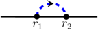
Figure 20: A 1-loop diagram representation of the linear order term (206) for distribution of positive time. We follow a similar convention as earlier. A dashed line indicates coupling between points $(r_{1},r_{2})$ (their order indicated by an arrowhead) with a coupling strength $e^{y(r_{1}-r_{2})}$ and a solid disk indicates a ‘charge’ of amplitude $\dot{x}(r)$ for the associated point $r$.

Using Eq. (10a) we write the linear order term (194b) as

$$W_{1}(\tau,T)= \,\frac{1}{2D}\int_{-\infty}^{\infty}dm\int_{0}^{\Lambda}dy\int_{0}^{T}dr_{1}\int_{r_{1}}^{T}dr_{2}\,$$

$$\qquad\times e^{y(r_{1}-r_{2})}\;\mathopen{\hbox{${\langle}$}\kern-2.72221pt\leavevmode\hbox{${\langle}$}}\dot{x}(r_{1})\dot{x}(r_{2})\mathclose{\hbox{${\rangle}$}\kern-2.72221pt\leavevmode\hbox{${\rangle}$}}_{(0,m)},$$ (206)

where the integral over time $r$ is interpreted as in Eq. (15). A graphical representation of the amplitude as a 1-loop diagram is sketched in Fig. 20.

To evaluate the conditional average in Eq. (206) we use a result for the correlation similar to Eq. (442). Generalizing the analysis in App. M for the conditioned case, we see that for $r_{2}>r_{1}$,

$$\mathopen{\hbox{${\langle}$}\kern-2.72221pt\leavevmode\hbox{${\langle}$}}\dot{x}(r_{1})\dot{x}(r_{2})\mathclose{\hbox{${\rangle}$}\kern-2.72221pt\leavevmode\hbox{${\rangle}$}}_{(m_{1},m_{2})}=2^{2}D^{2}\int\limits_{0}^{r_{1}}d\tau_{1}\int\limits_{0}^{r_{2}-r_{1}}d\tau_{2}$$

$$\times\int\limits_{0}^{T-r_{2}}d\tau_{3}\delta(\tau-\tau_{1}-\tau_{2}-\tau_{3})\int\limits_{-\infty}^{\infty}dx_{1}\,dx_{2}\,\mathbb{Z}_{r_{1}}(m_{1},x_{1}|\tau_{1})$$

$$\qquad\partial_{x_{1}}\mathbb{Z}_{r_{2}-r_{1}}(x_{1},x_{2}|\tau_{2})\partial_{x_{2}}\mathbb{Z}_{T-r_{2}}(x_{2},m_{2}|\tau_{3}).$$ (207)

This helps us to write $W_{1}(\tau,T)$ in terms of the conditional propagator $\mathbb{Z}$. By a change of variables and an integration by parts we obtain

$$W_{1}(\tau,T)=-2D\int\limits_{0}^{\infty}dt_{1}dt_{2}dt_{3}\int\limits_{0}^{t_{1}}d\tau_{1}\int\limits_{0}^{t_{2}}d\tau_{2}\int\limits_{0}^{t_{3}}d\tau_{3}$$ (208)

$$\times\delta(T{-}t_{1}{-}t_{2}{-}t_{3})\;\delta(\tau{-}\tau_{1}{-}\tau_{2}{-}\tau_{3})\int\limits_{0}^{\Lambda}dy\,e^{-y\,t_{2}}\int\limits_{-\infty}^{\infty}dm$$ (209)

$$\times\int\limits_{-\infty}^{\infty}dx_{1}dx_{2}\;\partial_{x_{1}}\mathbb{Z}_{t_{1}}(0,x_{1}|\tau_{1})\mathbb{Z}_{t_{2}}(x_{1},x_{2}|\tau_{2})$$ (210)

$$\qquad\times\partial_{x_{2}}\mathbb{Z}_{t_{3}}(x_{2},m|\tau_{3}).$$ (211)

A double Laplace transform Eq. (77) of the amplitude gives

$$\widetilde{W}_{1}(\lambda,s)=-2D\int\limits_{0}^{\Lambda}dy\int\limits_{-\infty}^{\infty}dx_{1}dx_{2}\partial_{x_{1}}\widetilde{\mathbb{Z}}_{s}(0,x_{1}|\lambda)$$ (212)

$$\qquad\times\widetilde{\mathbb{Z}}_{s+y}(x_{1},x_{2}|\lambda)\int\limits_{-\infty}^{\infty}dm\partial_{x_{2}}\widetilde{\mathbb{Z}}_{s}(x_{2},m|\lambda),$$ (213)

with $\widetilde{\mathbb{Z}}$ defined in Eq. (204).

Using the result (204) and integrating using integrals (499), (502), we get

$$\widetilde{W}_{1}(\kappa\,s,s)=\frac{\widetilde{\mathcal{A}}(1+\kappa)}{s\sqrt{1+\kappa}},$$ (214)

with

$$\widetilde{\mathcal{A}}(z)=\int\limits_{0}^{\Lambda/s}\frac{dy}{y^{2}}\left[\sqrt{z+y}-\sqrt{z}-\sqrt{1+y}+1\right]^{2},$$ (215)

which by mere coincidence happens to be the same integral as in Eq. (161), although their corresponding diagrams are different.

VIII.4 Quadratic order: 2-loop diagrams

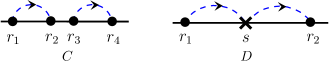
Figure 21: Two-loop diagrams for the quadratic order term $W_{2}$ for the distribution of positive time $t_{\rm pos}$. In this illustration we choose $r_{2}>r_{1}$ and $r_{4}>r_{3}$ for diagram $C$, whereas $r_{1}<s<r_{2}$ for diagram $D$. A solid disc denotes a ‘charge’ $\dot{x}(r)$ for the associated point $r$, whereas a cross denotes a contracted point with a ‘charge’ $2D$.

Following an analysis similar to that in Sec. VI.3, it is straightforward to see that for $W_{2}$ in Eq. (194c) contributions come only from the two diagrams shown in Fig. 21,

$$W_{2}(\tau,T)=C(\tau,T)+D(\tau,T),$$ (216)

where the amplitudes are given by

$$C(\tau,T)= \frac{1}{8D^{2}}\int_{-\infty}^{\infty}dm\int_{0}^{\Lambda}dy_{1}dy_{2}\int_{0}^{T}dr_{1}$$

$$\times\int_{r_{1}}^{T}dr_{2}\int_{0}^{T}dr_{3}\int_{r_{3}}^{T}dr_{4}e^{y_{1}(r_{1}-r_{2})}e^{y_{2}(r_{3}-r_{4})}$$

$$\times\mathopen{\hbox{${\big{\langle}}$}\kern-2.72221pt\leavevmode\hbox{${\big{\langle}}$}}\dot{x}(r_{1})\dot{x}(r_{2})\dot{x}(r_{3})\dot{x}(r_{4})\mathclose{\hbox{${\big{\rangle}}$}\kern-2.72221pt\leavevmode\hbox{${\big{\rangle}}$}}_{(0,m)}$$ (217)

and

$$D(\tau,T)=\frac{1}{2D} \int_{-\infty}^{\infty}dm\int_{0}^{\Lambda}dy_{1}dy_{2}\int_{0}^{T}dr_{1}\int_{r_{1}}^{T}ds$$ (218)

$$\times\int_{s}^{T}dr_{2} e^{y_{1}(r_{1}-s)}e^{y_{2}(s-r_{2})}\mathopen{\hbox{${\big{\langle}}$}\kern-2.72221pt\leavevmode\hbox{${\big{\langle}}$}}\dot{x}(r_{1})\dot{x}(r_{2})\mathclose{\hbox{${\big{\rangle}}$}\kern-2.72221pt\leavevmode\hbox{${\big{\rangle}}$}}_{(0,m)}.~{}~{}$$ (219)

These amplitudes can be expressed in terms of the conditional propagator $\mathbb{Z}_{T}$ in Eq. (197), and then an explicit result can be derived following an analysis similar to that of the linear-order term in Sec. VIII.3. Here we give their final expression, and defer their derivation to the App. J.

The double Laplace transform of the amplitude of the diagram $D$ in Fig. 21 can be written as

$$\widetilde{D}(\kappa\,s,s)=\frac{\widetilde{\mathcal{D}}(1+\kappa)}{s\sqrt{1+\kappa}},$$ (220)

where

$$\widetilde{\mathcal{D}}(z)=\frac{2}{(1+\sqrt{z})} \int_{0}^{\Lambda/s}\frac{dy_{1}dy_{2}}{y_{1}y_{2}}$$ (221)

$$\times\bigg{\{} \frac{y_{2}\,\mathfrak{h}(1,z,y_{1})}{(y_{2}-y_{1})}+\frac{y_{1}\,\mathfrak{h}(1,z,y_{2})}{(y_{1}-y_{2})}\bigg{\}}\qquad$$

with

$$\mathfrak{h} (s_{1},s_{2},y)=$$ (222)

$$\frac{\left(\sqrt{s_{2}+y}-\sqrt{s_{1}+y}\right)\left[\sqrt{s_{2}(s_{1}+y)}-\sqrt{s_{1}(s_{2}+y)}\right]}{(\sqrt{s_{1}+y}+\sqrt{s_{1}})(\sqrt{s_{2}+y}+\sqrt{s_{2}})}.$$

The double Laplace transform for the diagram $C$ in Fig. 21 is

$$\widetilde{C}(\kappa\,s,s)=\frac{\widetilde{\mathcal{C}}(1+\kappa)}{s\sqrt{1+\kappa}}$$ (223)

with

$$\widetilde{\mathcal{C}} (z)=\frac{4}{(1+\sqrt{z})}\int_{0}^{\Lambda/s}\frac{dy_{1}dy_{2}}{y_{1}y_{2}}\bigg{\{}\mathfrak{f}(1,z,y_{1},y_{2})+$$

$$\mathfrak{f}(z,1,y_{1},y_{2})+\frac{\mathfrak{g}(1,z,y_{1},y_{2})+\mathfrak{g}(z,1,y_{1},y_{2})}{y_{1}}\bigg{\}},$$ (224)

where we define

$$\mathfrak{g}(s_{1},s_{2},y_{1},y_{2})= \sqrt{{s_{1}}+y_{1}+y_{2}}\;\Big{(}\sqrt{{s_{2}}+y_{1}+y_{2}}-\sqrt{{s_{1}}+y_{1}+y_{2}}\Big{)}$$ (225)

$$\times \Big{(}\sqrt{{s_{1}}+y_{1}}+\sqrt{{s_{1}}+y_{2}}-\sqrt{{s_{1}}}+\sqrt{{s_{2}}+y_{1}+y_{2}}-\sqrt{{s_{2}}+y_{1}}-\sqrt{{s_{2}}+y_{2}}+\sqrt{{s_{2}}}\Big{)}$$ (226)

$$\times \left(\frac{\left(\sqrt{{s_{1}}}+\sqrt{{s_{2}}}\right)\left(-\sqrt{{s_{1}}}-\sqrt{{s_{2}}+y_{1}}+\sqrt{{s_{2}}}\right)}{\left(\sqrt{{s_{1}}+y_{1}}+\sqrt{{s_{2}}+y_{1}}\right)\left(\sqrt{{s_{1}}+y_{1}+y_{2}}+\sqrt{{s_{1}}+y_{1}}\right)}+\frac{\sqrt{{s_{1}}}}{\sqrt{{s_{1}}+y_{1}+y_{2}}+\sqrt{{s_{1}}}}\right)$$ (227)

$$+\left({s_{1}}+y_{2}\right) \Big{(}\sqrt{{s_{1}}+y_{2}}-\sqrt{{s_{2}}+y_{2}}\Big{)}\left(\frac{\left(\sqrt{{s_{1}}}+\sqrt{{s_{2}}}\right)\left(-\sqrt{{s_{1}}}-\sqrt{{s_{2}}+y_{1}}+\sqrt{{s_{2}}}\right)}{\left(\sqrt{{s_{1}}+y_{1}}+\sqrt{{s_{2}}+y_{1}}\right)\left(\sqrt{{s_{1}}+y_{1}}+\sqrt{{s_{1}}+y_{2}}\right)}+\frac{\sqrt{{s_{1}}}}{\sqrt{{s_{1}}+y_{2}}+\sqrt{{s_{1}}}}\right)$$ (228)

$$+\frac{1}{4}(s_{2}-s_{1})\Big{(}\sqrt{{s_{1}}+y_{1}}+\sqrt{{s_{1}}}-\sqrt{{s_{2}}+y_{1}}-\sqrt{{s_{2}}}\Big{)}$$ (229)

$$+\frac{\sqrt{{s_{1}}}\Big{(}\sqrt{{s_{1}}+y_{1}}-\sqrt{{s_{2}}+y_{1}}\Big{)}\Big{(}\sqrt{{s_{1}}}\left(\sqrt{{s_{2}}+y_{1}}-\sqrt{{s_{2}}}\right)+2{s_{1}}+y_{1}\Big{)}}{\sqrt{{s_{1}}+y_{1}}+\sqrt{{s_{1}}}},$$ (230)

and

$$\mathfrak{f}(s_{1},s_{2},y_{1},y_{2})= \frac{({s_{1}}+y_{2})}{y_{2}}\Big{(}\sqrt{{s_{2}}+y_{2}}-\sqrt{{s_{1}}+y_{2}}\Big{)}\left(\frac{\left(\sqrt{{s_{1}}}+\sqrt{{s_{2}}}\right)\left(\sqrt{{s_{2}}}-\sqrt{{s_{1}}}-\sqrt{{s_{2}}+y_{1}}\right)}{\left(\sqrt{{s_{1}}+y_{1}}+\sqrt{{s_{2}}+y_{1}}\right)\left(\sqrt{{s_{1}}+y_{1}}+\sqrt{{s_{1}}+y_{2}}\right)}+\frac{\sqrt{{s_{1}}}}{\sqrt{{s_{1}}+y_{2}}+\sqrt{{s_{1}}}}\right)$$ (231)

$$+\frac{\left(\sqrt{{s_{2}}}-\sqrt{{s_{1}}}\right)}{4y_{2}} \left(1+\frac{2\left(\sqrt{{s_{1}}}+\sqrt{{s_{2}}}\right)\left(\sqrt{{s_{2}}}-\sqrt{{s_{1}}}-\sqrt{{s_{2}}+y_{1}}\right)}{\left(\sqrt{{s_{1}}+y_{1}}+\sqrt{{s_{1}}}\right)\left(\sqrt{{s_{1}}+y_{1}}+\sqrt{{s_{2}}+y_{1}}\right)}\right)\Big{(}2\sqrt{{s_{1}}}\sqrt{{s_{2}}+y_{2}}-2\sqrt{{s_{1}}}\sqrt{{s_{2}}}-2\sqrt{{s_{1}}}\sqrt{{s_{1}}+y_{2}}-y_{2}\Big{)}$$ (232)

$$\qquad\qquad+\frac{\sqrt{{s_{1}}}\Big{(}\sqrt{{s_{2}}+y_{1}}-\sqrt{{s_{1}}+y_{1}}\Big{)}\Big{(}\sqrt{{s_{2}}}-\sqrt{{s_{1}}}-\sqrt{{s_{2}}+y_{1}}\Big{)}}{2\Big{(}\sqrt{{s_{1}}+y_{1}}+\sqrt{{s_{1}}}\Big{)}^{2}}.$$ (233)

Adding contribution of these two diagrams we get the double Laplace transform of the second order term

$$\widetilde{W}_{2}(\lambda,s)=\widetilde{C}(\lambda,s)+\widetilde{D}(\lambda,s).$$

The expressions in Eqs. (230) and (233) are given in the supplemental Mathematica notebook [76] for their numerical evaluation.

VIII.5 Result for $\mathcal{F}^{\rm pos}(\kappa,H)$

Rest of the analysis is very similar to that for $t_{\rm last}$ and $t_{\rm max}$. We write the amplitude $\widetilde{W}(\lambda,s)$ in Eq. (193) in an exponential form such that

$$\widetilde{W}(s\,\kappa,s)=\frac{e^{\widetilde{\mathcal{W}}(\kappa)}}{s\sqrt{1+\kappa}},$$ (234)

where $\widetilde{\mathcal{W}}=\varepsilon\,\widetilde{\mathcal{W}}_{1}+\varepsilon^{2}\,\widetilde{\mathcal{W}}_{2}+\cdots$, with

$$\widetilde{\mathcal{W}}_{1}(\kappa)= \;\widetilde{\mathcal{A}}(1+\kappa),$$ (235a)

$$\widetilde{\mathcal{W}}_{2}(\kappa)= \;\widetilde{\mathcal{C}}(1+\kappa)+\widetilde{\mathcal{D}}(1+\kappa)-\frac{1}{2}\widetilde{\mathcal{A}}(1+\kappa)^{2}.$$ (235b)

Considering the normalization in Eq. (192) we get the Laplace transform of the distribution of $t_{\rm pos}$ in Eq. (83) with

$$\widetilde{\mathcal{F}}^{\rm pos}(\kappa,H)=\widetilde{\mathcal{W}}(\kappa)-\widetilde{\mathcal{W}}(0).$$ (236)

One can verify that $\widetilde{\mathcal{W}}(0)=0$ up to the second order in the perturbation expansion, and this means in the expansion Eq. (86a),

$$\widetilde{\mathcal{F}}_{1}^{\rm pos}(\kappa)=\widetilde{\mathcal{W}}_{1}(\kappa)\quad\text{and}\quad\widetilde{\mathcal{F}}_{2}^{\rm pos}(\kappa)=\widetilde{\mathcal{W}}_{2}(\kappa).$$ (237)

Comparing with Eq. (175) we see that $\widetilde{\mathcal{F}}_{1}^{\rm pos}(\kappa)$ is exactly same as $\widetilde{\mathcal{F}}_{1}^{\rm max}(\kappa)$, and therefore we get

$$\mathcal{F}_{1}^{\rm pos}(\vartheta)=\mathcal{F}_{1}^{\rm max}(\vartheta)$$ (238)

given in Eq. (179).

The difference with the distribution for $t_{\rm max}$ comes in the second order term. This is given by

$$\mathcal{F}_{2}^{\rm pos}(\vartheta)= -\frac{1}{2}\left[\mathcal{F}_{1}^{\rm pos}(\vartheta)-\mathcal{R}^{\rm pos}(\vartheta)\right]^{2}$$ (239)

$$+\mathcal{K}_{\kappa\rightarrow\vartheta}^{-1}\odot\left[\widetilde{\mathcal{F}}_{2}^{\rm pos}(\kappa)+\frac{1}{2}\widetilde{\mathcal{F}}_{1}^{\rm pos}(\kappa)^{2}\right].$$ (240)

Following a similar analysis as used for Eq. (190) we get our result

$$\mathcal{F}_{2}^{\rm pos}(\vartheta) =-\frac{1}{2}\psi_{2}\left(\sqrt{\frac{\vartheta}{1-\vartheta}}\right)^{2}+$$ (241)

$$\mathcal{K}_{\kappa\rightarrow\vartheta}^{-1} \odot\left[\widetilde{\mathcal{C}}(1+\kappa)+\widetilde{\mathcal{D}}(1+\kappa)-\frac{1}{2}\widetilde{\mathcal{A}}(1+\kappa)^{2}\right]\quad$$ (242)

with Eq. (189).

It is difficult to analytically do the integration for the amplitudes in the second term in Eq. (242). We have numerically verified that the term remains finite for $\Lambda\to\infty$. For an explicit formula in terms of $\vartheta$ we exchange the order of $\mathcal{K}_{\kappa\rightarrow\vartheta}^{-1}$-transformation and the integration. This allows us to write

$${\cal F}^{\rm pos}_{2}(\vartheta)= -\frac{1}{2}\psi_{2}\left(\sqrt{\frac{\vartheta}{1-\vartheta}}\right)^{2}$$ (243)

$$+2\int_{0}^{\infty}\frac{dy_{1}dy_{2}}{y_{1}^{2}y_{2}^{2}}\;\Psi^{\rm pos}\left(y_{1},y_{2},\frac{1-\vartheta}{\vartheta}\right).$$

Expression for $\Psi^{\rm pos}$ is lengthy and it is given in the Appendix K. Our result for ${\cal F}^{\rm pos}_{2}(\vartheta)$ is plotted in Fig. 7, which agrees well with our computer simulation result. For this we evaluated both the ${\cal K}^{-1}$-transformation and the $y$-integration numerically.

IX Summary

We found a generalization of the three arc-sine laws of Brownian motion for an fBm. Unlike in the Brownian motion, the probabilities are different and given in Eqs. (49)-(48). These results are obtained using a perturbation expansion around the Brownian motion, and by a scaling argument for divergences near $\vartheta\to 0$ and $1$. Our numerical simulations confirm these highly non-trivial predictions accurately. We find a very good convergence to the numerical results for the entire range of $\vartheta$ even for large $\varepsilon$. Most realizations of fBm found in practical applications fall within the range $H\simeq\tfrac{1}{2}\pm 0.25$ where our formulas yield high-precision predictions.

Our perturbation approach offers a systematic framework to obtain analytical results for other observables of an fBm, of which very few are available so far. For example, distribution of Area under a Brownian excursion is known to have an Airy distribution [77]. Corresponding generalization for an fBm is yet unavailable. On simpler examples, a closed form expression for an fBm propagator with absorbing and reflecting boundary is desirable.

Appendix A Perturbation expansion of the fBm action

Writing $H=\frac{1}{2}+\varepsilon$ in the expression for $G^{-1}(t_{1},t_{2})=\langle X_{t_{1}}X_{t_{2}}\rangle$ given in Eq. (1) and expanding in powers of small $\varepsilon$ we get

$$G^{-1}(t_{1},t_{2})=K_{0}(t_{1},t_{2})+\varepsilon K_{1}(t_{1},t_{2})+\varepsilon^{2}K_{2}(t_{1},t_{2})+\cdots,$$

where

$$K_{0}(t_{1},t_{2})\equiv G_{0}^{-1}(t_{1},t_{2})=2\min(t_{1},t_{2}),$$

and, for $n\geq 1$,

$$K_{n}(t_{1},t_{2})=\frac{2^{n}}{n!}\bigg{[}t_{1}\ln^{n}t_{1} +t_{2}\ln^{n}t_{2}$$ (244)

$$- |t_{1}-t_{2}|\ln^{n}|t_{1}-t_{2}|\bigg{]}.\qquad$$ (245)

For $G$ related by $G^{-1}\,G(t_{1},t_{2})=G\,G^{-1}(t_{1},t_{2})=\delta(t_{1}-t_{2})$, this is equivalent to a perturbation expansion

$$G(t_{1},t_{2})=G_{0}(t_{1},t_{2})+\varepsilon\,G_{1}(t_{1},t_{2})+\varepsilon^{2}\,G_{2}(t_{1},t_{2})+\cdots$$

with

$$G_{0}(t_{1},t_{2})=-\frac{1}{2}\delta^{\prime\prime}(t_{1}-t_{2}),$$ (246a)

and for $$n\geq 1$$,

$$G_{n}(t_{1},t_{2})=-\sum_{q=1}^{n}G_{0}K_{q}G_{n-q}(t_{1},t_{2}).$$ (246b)

(Here we denote

$$AB(t_{1},t_{2})=\int_{0}^{T}ds\;A(t_{1},s)B(s,t_{2}),$$ (247)

for any two bivariate functions $A$ and $B$.)

It will be convenient for our analysis to write $G_{n}$ in Eq. (246) as

$$G_{n}=G_{0}\Sigma_{n}G_{0}$$ (248)

for all positive integers $n$, such that

$$\Sigma_{0} =K_{0},\quad\Sigma_{1}=-K_{1},\quad\Sigma_{2}=-K_{2}+K_{1}G_{0}K_{1},$$

$$\Sigma_{3}= -K_{3}+K_{2}G_{0}K_{1}+K_{1}G_{0}K_{2}-K_{1}G_{0}K_{1}G_{0}K_{1},$$ (249)

and so on. In terms of this perturbation expansion, action (5) is written as

$$S=S_{0}+\varepsilon\,\mathcal{L}_{1}+\varepsilon^{2}\mathcal{L}_{2}+\cdots,$$ (250)

where $S_{0}$ is in Eq. (8a) and for $n\geq 1$,

$$\mathcal{L}_{n}=\int_{0}^{T}dt_{1}\int_{0}^{T}dt_{2}\;\dot{x}(t_{1})\left\{\frac{1}{8}\partial_{t_{1}}\partial_{t_{2}}\Sigma_{n}(t_{1},t_{2})\right\}\,\dot{x}(t_{2})$$ (251)

obtained by integration by parts.

For their explicit expression we use the following results obtained from Eq. (245): for $t_{2}\geq t_{1}$

$$\frac{1}{4}\partial_{t_{1}}\partial_{t_{2}} K_{1}=(1+\ln\omega)\delta(t_{1}-t_{2})+\frac{1}{2}\frac{1}{(t_{2}-t_{1})},$$ (252a)

$$\frac{1}{4}\partial_{t_{1}}\partial_{t_{2}} K_{2}=\left(\frac{\pi^{2}}{6}+2\ln\omega+\ln^{2}\omega\right)\delta(t_{1}-t_{2})$$ (252b)

$$+\frac{1+\ln\omega}{(t_{2}-t_{1})}+\frac{1}{2}\int_{t_{1}+\omega}^{t_{2}-\omega}\frac{ds}{(t_{2}-s)(s-t_{1})},$$ (252c)

where singularities are regularized by introducing an infinitesimally small ultraviolet cutoff $$\omega>0 \delta(t_{1}-t_{2})\ln(t_{2}-t_{1})\simeq\delta(t_{1}-t_{2})\ln\omega$$ in time, such that terms like and

$$\frac{\ln(t_{2}-t_{1})}{(t_{2}-t_{1})}\simeq \frac{\ln\omega}{(t_{2}-t_{1})}+\frac{\pi^{2}}{6}\delta(t_{1}-t_{2})$$ (252d)

$$+\frac{1}{2}\int_{t_{1}+\omega}^{t_{2}-\omega}\frac{ds}{(t_{2}-s)(s-t_{1})},$$ (252e)

which are used for writing Eq. (252c). Similarly, for $$t_{2}\geq t_{1}$$,

$$\frac{1}{4}\partial_{t_{1}}\partial_{t_{2}} K_{1}G_{0}K_{1}=2\left(1+\ln\omega\right)^{2}\delta(t_{1}-t_{2})$$ (252f)

$$+\frac{2(1+\ln\omega)}{(t_{2}-t_{1})}+\frac{1}{2}\int_{0}^{T}\frac{ds}{|t_{1}-s||t_{2}-s|}.$$ (252g)

Using Eq. (252) in Eq. (249) and Eq. (251) it is easy to see that

$$\mathcal{L}_{1}= -2(1+\ln\omega)S_{0}-\frac{1}{2}S_{1},$$ (253a)

$$\mathcal{L}_{2}= \left[2\left(1-\frac{\pi^{2}}{6}\right)+2\left(1+\ln\omega\right)^{2}\right]S_{0}$$

$$\qquad\qquad+\left(1+\ln\omega\right)S_{1}+S_{2},$$ (253b)

where $$S_{0} S_{1} S_{2}$$, , and are defined in Eq. (8). The expansion (250) with Eq. (253) gives Eq. (7).

Appendix B Alternate derivation of the action

Here we give an elegant and short derivation of the action in Eqs. (7)-(8) in a normal-ordered form. Using integration by parts, Eq. (5) gives

$$S[X_{t}]=\frac{1}{2}\int_{0}^{T}dt_{1}\int_{0}^{T}dt_{2}\;\dot{X}_{t_{1}}C^{-1}(t_{1},t_{2})\dot{X}_{t_{2}}$$ (254)

with the correlation

$$C(t_{1},t_{2})= \langle\dot{X}_{t_{1}}\dot{X}_{t_{2}}\rangle=4H|t_{1}-t_{2}|^{2H-1}\delta(t_{1}-t_{2})$$

$$\qquad+2H(2H-1)|t_{1}-t_{2}|^{2(H-1)}.$$ (255)

An expansion in $\varepsilon=H-\frac{1}{2}$ gives

$$C(t_{1},t_{2})=2\widehat{D} \left[\delta(t_{1}-t_{2})+\varepsilon\frac{1}{|t_{1}-t_{2}|}\right.$$

$$\qquad\quad\left.+\varepsilon^{2}\frac{2\ln\frac{|t_{1}-t_{2}}{\omega}}{|t_{1}-t_{2}|}+\cdots\right],$$ (256)

with $\widehat{D}=2H\omega^{2H-1}=(1+2\varepsilon)\omega^{2\varepsilon}$, and $\omega$ being an ultraviolet cutoff in time. This implies

$$C^{-1} (t_{1},t_{2})=\frac{1}{2\widehat{D}}\left[\delta(t_{1}-t_{2})-\frac{\varepsilon}{|t_{1}-t_{2}|}\right.$$

$$\left.-\varepsilon^{2}\frac{2\ln\frac{|t_{1}-t_{2}|}{\omega}}{|t_{1}-t_{2}|}+\varepsilon^{2}\int ds\frac{1}{|s-t_{1}||s-t_{2}|}+\cdots\right].$$

Substituting in Eq. (254) and defining a normal-ordered form (non-contact terms only) in Eq. (16) we get

$$\mathcal{S}^{(n)}[X_{t}]=\frac{1}{2\widehat{D}} \int_{t1<t_{2}}dt_{1}dt_{2}\dot{X}_{t_{1}}\dot{X}_{t_{2}}\bigg{[}\delta(t_{1}-t_{2})$$

$$-\frac{\varepsilon}{|t_{1}-t_{2}|}-2\varepsilon^{2}\frac{\ln\frac{|t_{1}-t_{2}|}{\omega}}{|t_{1}-t_{2}|}+\cdots\bigg{]}.$$ (257)

Using the integral representation Eq. (252e) this gives

$$\mathcal{S}^{(n)} [X_{t}]=\frac{1}{2D}\int_{t1<t_{2}}dt_{1}dt_{2}\dot{X}_{t_{1}}\dot{X}_{t_{2}}\bigg{[}\delta(t_{1}-t_{2})$$

$$-\frac{\varepsilon}{|t_{1}-t_{2}|}-\varepsilon^{2}\int_{t_{1}}^{t_{2}}ds\frac{1}{|s-t_{1}||s-t_{2}|}+\cdots\bigg{]},$$ (258)

with $D$ given in Eq. (9). Comparing with Eqs. (7)-(8) one can see that the both leading and sub-leading terms are same whereas the $\varepsilon^{2}$ order term includes only contact-less terms. An integral representation of the normal-ordered second-order term is in Eq. (17).

Appendix C The fBm propagator

Here, we verify Eq. (18) using the perturbation expansion of the action (250) to all orders. In terms of this expansion, Eq. (20a) can be written as

$$W_{H}(m,T)=\left\langle e^{-\sum_{n\geq 1}\varepsilon^{n}\mathcal{L}_{n}}\right\rangle,$$ (259)

where by the angular brackets we denote (definition restricted only for this Appendix)

$$\left\langle O[x]\right\rangle\equiv\int_{x(0)=0}^{x(T)=m}\mathcal{D}[x]\;e^{-S_{0}}O[x].$$ (260)

Then, using a result for the multi-time correlation given later in Eq. (453) for $D=1$ and the propagator Eq. (20a) leads to

$$\mathcal{G}_{H}(m,T)=e^{F(T)\partial_{m}^{2}}\mathcal{G}(m,T)$$ (261)

with

$$F(T)=\frac{1}{2}\int_{0}^{T}dt_{1}\int_{0}^{T}dt_{1}\sum_{n\geq 1}\varepsilon^{n}\partial_{t_{1}}\partial_{t_{2}}K_{n}(t_{1},t_{2}),$$ (262)

where we used Eq. (249) and Eq. (251).

• In Eq. (261), the contribution from terms like $K_{1}G_{0}K_{1}$ etc in Eq. (249) are canceled from the terms in normalization $N_{T}$ in Eq. (18). One may explicitly verify this at lower orders in perturbation expansion.

Using Eq. (245) in Eq. (262), it is easy to see that

$$F(T)=T\sum_{n\geq 1}\frac{(2\varepsilon\ln T)^{n}}{n!}=T(T^{2\varepsilon}-1),$$ (263)

which in Eq. (261) leads to

$$\mathcal{G}_{H}(m,T)=e^{(T^{2H}-T)\partial_{m}^{2}}\mathcal{G}(m,T),$$ (264)

where we used $1+2\varepsilon=2H$. Using the expression of $\mathcal{G}(m,T)$ in Eq. (25), it is now easy to obtain Eq. (18).

Appendix D Numerical simulation of an fBm

Efficient computer simulation of an fBm trajectory is a delicate task. A vast literature has been published on this subject. For a comparative study of many of the sampling methods for an fBm see the review [78] and references therein. In general these algorithms generate the full trajectory. If one is only interested in a specific observable, as the first-passage time, not all points need to be generated, allowing for tremendous gains both in memory usage and execution speed [72, 73, 66].

In our work, we use a discrete-time sampling method following the Davis and Harte procedure [70] (also known as the Wood and Chan procedure [79]) as described in Ref. [71]. The basic idea is to construct fBm paths from a discrete-time sampling of stationary, Gaussian-distributed, increments $\Delta X_{n}$ for integers $n=0,1,\cdots,N-1$, with mean $\langle\Delta X_{n}\rangle=0$ and covariance

$$\langle\Delta X_{m}\Delta X_{n}\rangle=\gamma(m-n)$$ (265)

$$\quad=(m-n+1)^{2H}+(m-n-1)^{2H}-2(m-n)^{2H},$$

for positive integers $n\leq m<N$. For large $N$ with $t=n/N$, one can see that $N^{2-2H}\gamma(Nt-Ns)$ converge to the covariance (2). This means, the cumulated sum $N^{-H}\sum_{i=0}^{n}\Delta X_{i}$ for large $N$ gives an fBm path $X_{t}$ with $X_{0}=0$ in a time window $[0,1]$.

The Davis and Harte procedure is an efficient algorithm for generating samples of $\Delta X_{n}$ with a computational efficiency $\mathcal{O}(N\ln N)$ (compared to $\mathcal{O}(N^{3})$ for Choleski decomposition method [78]). The algorithm involves the following simple steps. We construct two linear arrays $\{W_{n}\}$ and $\{\lambda_{n}\}$ of length $2N$ with index $n=0,1,\cdots,2N-1$. Elements of the first array are generated from a set of $2N$ independent Gaussian random numbers ${V_{0},V_{1},\cdots,V_{2N-1}}$, with $\langle V_{n}\rangle=0$ and $\langle V_{m}V_{n}\rangle=\delta_{m,n}$. We define

$$W_{0}=V_{0},\qquad W_{n}=\frac{1}{\sqrt{2}}\left(V_{n}+i\;V_{2N-n}\right),$$ (266)

for $n=1,\cdots,N-1$, whereas

$$W_{N}=V_{N},\qquad W_{n}=\frac{(-i)}{\sqrt{2}}\left(V_{n}+i\;V_{2N-n}\right),$$ (267)

for $n=N+1,\cdots,2N-1$. This construction ensures that $\langle W_{n}\rangle=0$ and

$$\langle W_{k}W_{k^{\prime}}\rangle=\delta_{k,0}\delta_{k^{\prime},0}+\delta_{k+k^{\prime},2N},$$ (268)

for indices $0\leq k\leq 2N-1$.

Elements of the second array are defined by

$$\lambda_{n}=\sum_{k=0}^{2N-1}\Gamma_{k}\;e^{i\,\pi\frac{nk}{N}}$$ (269)

for integers $0\leq n\leq 2N-1$, where $\Gamma_{k}=\gamma(k)$ for $0\leq k\leq N$ and $\Gamma_{k}=\gamma(2N-k)$ for $N+1\leq k\leq 2N-1$ with covariance in Eq. (265). This means,

$$\lambda_{2N-n}=\lambda_{n}$$ (270)

and the inversion formula

$$\Gamma_{k}=\frac{1}{2N}\sum_{n=0}^{2N-1}\lambda_{n}\;e^{-i\,\pi\frac{nk}{N}}.$$ (271)

The set of increments for a discrete fBm are obtained from

$$\Delta X_{n}=\frac{1}{\sqrt{2N}}\sum_{k=0}^{2N-1}W_{k}\;\sqrt{\lambda_{k}}\;e^{i\pi\frac{nk}{N}}$$ (272)

for $0\leq n\leq N-1$. In comparison, we shall see that the set of increments for $N\leq n\leq 2N-1$ do not have the covariance (265) and they are discarded.

It is simple to verify that this construction (272) indeed generates Gaussian random numbers with covariance (265). The simplest is to see that $\langle\Delta X_{n}\rangle=0$ from $\langle W_{n}\rangle=0$. Moreover, $X_{n}$ is a linear combination of Gaussian random variables $W_{n}$, and therefore it’s distribution remains Gaussian. For the covariance, using Eq. (272) we write

$$\langle\Delta X_{m}\Delta X_{n}\rangle=\frac{1}{2N}\sum_{k,k^{\prime}=0}^{2N-1}\langle W_{k}W_{k^{\prime}}\rangle\;\sqrt{\lambda_{k}\lambda_{k^{\prime}}}\;e^{\frac{i\pi}{N}\left(nk+mk^{\prime}\right)},$$

which using Eq. (268) gives

$$\langle\Delta X_{m}\Delta X_{n}\rangle=\frac{1}{2N}\left\{\lambda_{0}+\sum_{k=1}^{2N-1}\sqrt{\lambda_{k}\lambda_{2N-k}}\;e^{-i\frac{\pi}{N}\left(m-n\right)k}\right\},$$ (273)

for $n\leq m$. Using the symmetry in Eq. (270) the above expression simplifies to

$$\langle\Delta X_{m}\Delta X_{n}\rangle= \frac{1}{2N}\sum_{k=1}^{2N-1}\lambda_{k}\;e^{-i\frac{\pi}{N}\left(m-n\right)k},$$ (274)

$$= \Gamma_{m-n}$$ (275)

for $m\geq n$, where in the last step we used the inverse Fourier transformation (271). It is clear from Eq. (275) that,

$$\langle\Delta X_{m}\Delta X_{n}\rangle=\gamma(m-n)\quad\text{for }m-n\leq N,$$ (276)

which includes all $0\leq n\leq m\leq N-1$. For indices $\geq N$, such that $m-n>N$, the covariance is $\gamma(2N-m+n)$, and therefore $\Delta X_{n}$ for $n\geq N$ are discarded.

The mathematics behind this algorithm is clearly explained in [78, 71]. It involves calculating square root of a positive matrix by embedding it in a circulant matrix. We shall not repeat the discussion this here. Reader may find details in [78, 71].

Appendix E A derivation of the inverse transform

The inverse transformation in Eq. (80) can be derived using complex analysis by writing Eq. (79) as

$$\widetilde{p}(z)=\oint_{\mathcal{C}}d\ell\frac{p(\ell)}{1+z\ell},$$

where $C$ is a simple closed contour drawn in Fig. 22. In an alternative representation

$$\frac{1}{2\pi i}\oint_{\mathcal{C}}d\ell\frac{p(\ell)}{\ell-z}=f(z):=\frac{1}{2\pi i}\left(-\frac{1}{z}\right)\widetilde{p}\left(-\frac{1}{z}\right).$$ (277)

The Sokhotski-Plemlj formula of complex analysis gives the inverse transformation

$$p(\ell)=f_{+}(\ell)-f_{-}(\ell)$$ (278)

for any point $\ell$ on the contour $C$, where $f_{\pm}(\ell)=\lim_{z\rightarrow\ell}f(z)$ with the limit taken from the domain inside (+) and outside (-) the contour $C$, respectively. For $\ell=\vartheta$ on the real axis,

$$f_{\pm}(\vartheta)=-\frac{1}{2\pi i\,\vartheta}\lim_{\delta\rightarrow 0}\widetilde{p}\left(-\frac{1}{\vartheta}\pm i\delta\right)$$ (279)

and this gives Eq. (80).

Figure 22: Contour $C$ for the complex integral (E).

Appendix F A list of useful $\mathcal{K}^{-1}$ transforms

Here, we give functions, which are related by the transformation Eq. (85) and its inverse transformation Eq. (87). These relations, indicated below by $\leftrightarrow$, are useful for our analysis. They can be numerically verified in Mathematica. A trivial, but useful result is $1\leftrightarrow 1$.

Among others,

$$-2\ln\left[1+\sqrt{1+\kappa}\right]\leftrightarrow\ln\vartheta,$$ (280)

$$-2\ln\left[1+\frac{1}{\sqrt{1+\kappa}}\right]\leftrightarrow\ln(1-\vartheta),$$ (281)

which using linearity of the transformation leads to

$$\ln(1+\kappa)-4\ln\left[1+\sqrt{1+\kappa}\right]\leftrightarrow\ln\vartheta(1-\vartheta),$$ (282)

and

$$-\ln(1+\kappa)\leftrightarrow\ln\frac{\vartheta}{1-\vartheta}.$$ (283)

Additionally,

$$\left(\ln(1+\kappa)\right)^{2}\leftrightarrow\left(\ln\frac{\vartheta}{1-\vartheta}\right)^{2}-\pi^{2}.$$ (284)

We get,

$$\frac{\ln(1+\sqrt{1+\kappa})}{\sqrt{1+\kappa}}\leftrightarrow x\arctan\frac{1}{x},$$ (285)

and

$$\sqrt{1+\kappa}\ln(1+\frac{1}{\sqrt{1+\kappa}})\leftrightarrow\frac{1}{x}\arctan x,$$ (286)

where $x=\sqrt{\frac{\vartheta}{1-\vartheta}}$. A linear combination of Eqs. (281, 285, 286) gives

$$- \left(1+\sqrt{1+\kappa}\right)\ln(1+\kappa)+\frac{2\left(1+\sqrt{1+\kappa}\right)^{2}}{\sqrt{1+\kappa}}$$

$$\qquad\times\ln\left(1+\sqrt{1+\kappa}\right)\leftrightarrow\psi(x)-\ln\vartheta(1-\vartheta)$$ (287)

with Eq. (51c) and the same definition for $x$. A related result about square of the above function is

$$\Big{[}-\left(1+\sqrt{1+\kappa}\right)\ln(1+\kappa)+\frac{2\left(1+\sqrt{1+\kappa}\right)^{2}}{\sqrt{1+\kappa}}\times$$ (288)

$$\ln\left(1+\sqrt{1+\kappa}\right)\Big{]}^{2}\leftrightarrow\left[\psi(x)-\ln\vartheta(1-\vartheta)\right]^{2}-\psi_{2}(x)^{2}.\qquad$$ (289)

with Eqs. (51c) and (189).

Other results, useful for verifying Eqs. (55, 57, 60), are

$$\frac{\Gamma\left(\frac{n}{2}\right)}{\sqrt{\pi}}\;{}_{2}F_{1}\left(\frac{1}{2},\frac{n-1}{2},\frac{n+1}{2},-\kappa\right)\leftrightarrow(\vartheta)^{\frac{n-1}{2}},$$ (290)

$$\frac{\sqrt{1+\kappa}\;\Gamma\left(\frac{n}{2}\right)}{\sqrt{\pi}}\;{}_{2}F_{1}\left(\frac{1}{2},1,\frac{n+1}{2},-\kappa\right)\leftrightarrow(1-\vartheta)^{\frac{n-1}{2}},$$ (291)

and their product

$$\frac{\sqrt{1+\kappa}\;\Gamma\left(\frac{n}{2}\right)^{2}}{\sqrt{\pi}}\;{}_{2}F_{1}\left(1,\frac{n}{2},n,-\kappa\right)\leftrightarrow\left[\vartheta(1-\vartheta)\right]^{\frac{n-1}{2}},$$ (292)

for $n\geq 1$, where ${}_{2}F_{1}(a,b,c,z)/\Gamma(c)$ is regularized hypergeometric function and it can be evaluated to arbitrary numerical precision in Mathematica.

Appendix G Amplitude of the Two-loop diagrams for $t_{\rm last}$

Here, we give a detailed derivation of the amplitudes of 2-loop diagrams shown in Fig. 14.

G.1 Non-trivial diagram D contributing to $\mathcal{F}^{\rm last}$.

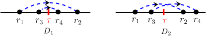
Figure 23: Two distinct cases of the 2-loop diagram $D$ in Fig. 14 for distribution of $t_{\rm last}$, categorized according to whether loops intersect (for $D_{1}$) or not (for $D_{2}$). The time variables $r$’s remain on the same side of $\tau$ as indicated.

Amplitude of the diagram $D$ in Fig. 14 is given by

$$D(\tau,T)=\frac{1}{4D^{2}}\int_{0}^{\infty}dm\int_{0}^{\Lambda}dy_{1}dy_{2}\int_{0}^{\tau}dr_{1}\int_{\tau}^{T}dr_{2}\int_{0}^{\tau}dr_{3}$$

$$\times\int_{\tau}^{T}dr_{4}\,e^{y_{1}(r_{1}-r_{2})}e^{y_{2}(r_{3}-r_{4})}\mathopen{\hbox{${\Big{\langle}}$}\kern-2.72221pt\leavevmode\hbox{${\Big{\langle}}$}}\dot{x}(r_{1})\dot{x}(r_{2})\dot{x}(r_{3})\dot{x}(r_{4})\mathclose{\hbox{${\Big{\rangle}}$}\kern-2.72221pt\leavevmode\hbox{${\Big{\rangle}}$}}_{m}$$

with the angular brackets defined in Eq. (97). Considering order of the time variables, the possible cases are illustrated in Fig. 23. Their amplitude can be expressed in terms of $J$ and $J^{+}$ defined in Eq. (107). Adding them, we write

$$D(\tau,T)= \frac{2}{4D^{2}}\!\int_{0}^{\infty}dm\!\!\int_{0}^{\Lambda}dy_{1}dy_{2}e^{-\tau(y_{1}+y_{2})}J_{\tau}(0,x_{0};-y_{1},-y_{2})$$

$$\times\Big{[}J_{T-\tau}^{+}(x_{0},m;y_{2},y_{1})+J_{T-\tau}^{+}(x_{0},m;y_{1},y_{2})\Big{]},$$

where the pre-factor $2$ is due to interchange of pairs $(r_{1},r_{2})$ with $(r_{3},r_{4})$.

Its double Laplace transformation in Eq. (77) gives

$$\widetilde{D}(\lambda,s)= \frac{1}{2D^{2}}\!\int_{0}^{\infty}dm\!\!\int_{0}^{\Lambda}dy_{1}dy_{2}\widetilde{J}_{s+\lambda+y_{1}+y_{2}}(0,x_{0};-y_{1},-y_{2})$$

$$\times\left[\widetilde{J}_{s}^{+}(x_{0},m;y_{2},y_{1})+\widetilde{J}_{s}^{+}(x_{0},m;y_{1},y_{2})\right].$$

It is convenient to write the expression in a form such that the integrand is symmetric in $y_{1}$ and $y_{2}$. We write

$$\widetilde{D}(\lambda,s)=\frac{1}{4D^{2}}\int_{0}^{\Lambda}dy_{1}dy_{2}\bigg{[}\widetilde{J}_{s+\lambda+y_{1}+y_{2}}(0,x_{0};$$ (293)

$$-y_{1},-y_{2})+\widetilde{J}_{s+\lambda+y_{1}+y_{2}}(0,x_{0};-y_{2},-y_{1})\bigg{]}\times$$ (294)

$$\int_{0}^{\infty}dm\bigg{[}\widetilde{J}_{s}^{+}(x_{0},m;y_{2},y_{1})+\widetilde{J}_{s}^{+}(x_{0},m;y_{1},y_{2})\bigg{]}.$$ (295)

We show that (a derivation given in App. N)

$$\widetilde{J}_{s}(m_{1},m_{2} ;y_{1},y_{2})=\frac{2\sqrt{D}}{y_{1}y_{2}(y_{1}+y_{2})}\Bigg{[}y_{1}\sqrt{s}\;e^{-z\sqrt{s}}$$

$$\qquad+y_{2}\sqrt{s+y_{1}+y_{2}}\;e^{-z\sqrt{s+y_{1}+y_{2}}}$$ (296)

$$\qquad\quad-(y_{1}+y_{2})\sqrt{s+y_{2}}\;e^{-z\sqrt{s+y_{2}}}\Bigg{]},$$ (297)

where $z=\tfrac{|m_{1}-m_{2}|}{\sqrt{D}}$ and

$$\int_{0}^{\infty} dm_{2}\widetilde{J}_{s}^{+}(m_{1},m_{2};y_{1},y_{2})$$ (298)

$$=\frac{4D}{y_{1}y_{2}}\sqrt{\frac{s+y_{2}}{s}}\left[e^{-m_{1}\sqrt{\frac{s+y_{2}}{D}}}-e^{-m_{1}\sqrt{\frac{s+y_{1}+y_{2}}{D}}}\right]$$ (299)

$$\quad+\frac{4D}{(y_{1}+y_{2})y_{2}}\left[e^{-m_{1}\sqrt{\frac{s+y_{1}+y_{2}}{D}}}-e^{-m_{1}\sqrt{\frac{s}{D}}}\right].\qquad$$ (300)

Using the asymptotic of (297) for small $x_{0}$, we obtain

$$\widetilde{J}_{s} (0,x_{0};-y_{1},-y_{2})+\widetilde{J}_{s}(0,x_{0};-y_{2},-y_{1})\simeq$$

$$\frac{2\sqrt{D}}{y_{1}y_{2}}\bigg{(}\sqrt{s}-\sqrt{s-y_{2}}-\sqrt{s-y_{1}}+\sqrt{s-y_{1}-y_{2}}\bigg{)}$$

and similarly from Eq. (300) we get for small $x_{0}$,

$$\int_{0}^{\infty} dm\bigg{\{}\widetilde{J}_{s}^{+}(x_{0},m;y_{2},y_{1})+\widetilde{J}_{s}^{+}(x_{0},m;y_{1},y_{2})\bigg{\}}$$

$$\simeq-\frac{4x_{0}\sqrt{D}}{y_{1}y_{2}}\times\frac{\sqrt{s+y_{1}+y_{2}}}{\sqrt{s}}\times$$ (301)

$$\bigg{(}\sqrt{s+y_{1}+y_{2}}-\sqrt{s+y_{1}}-\sqrt{s+y_{2}}+\sqrt{s}\bigg{)}.\quad$$ (302)

Using these asymptotics in Eq. (295) we get, for small $x_{0}$,

$$\widetilde{D}(\lambda,s)\simeq-\frac{2x_{0}}{D} \int_{0}^{\Lambda}\frac{dy_{1}dy_{2}}{y_{1}^{2}y_{2}^{2}}\times\frac{\sqrt{s+y_{1}+y_{2}}}{\sqrt{s}}\times$$

$$\bigg{(}\sqrt{s+y_{1}+y_{2}} -\sqrt{s+y_{1}}-\sqrt{s+y_{2}}+\sqrt{s}\bigg{)}$$

$$\times\bigg{(}\sqrt{s+\lambda+y_{1}+y_{2}} -\sqrt{s+\lambda+y_{1}}$$

$$-\sqrt{s+\lambda+y_{2}}+\sqrt{s+\lambda}\bigg{)}.$$

This leads to the result in terms of re-scaled arguments in Eq. (120) and Eq. (121).

G.2 Two-loop diagrams contributing to simple scaling

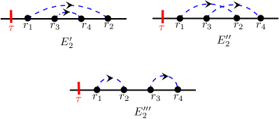
Figure 24: Diagram $E_{2}$ of Fig. 14 is made of three cases according to relative order of time variables with $r_{1}<r_{2}$ and $r_{3}<r_{4}$, remaining on the side of $\tau$ as indicated.

G.2.1 Diagrams $E_{1}$ and $E_{2}$

We begin with the diagram $E_{2}$ in Fig. 14, whose amplitude is given by

$$E_{2}(\tau,T)=\frac{1}{4D^{2}}\int_{0}^{\infty}dm\int_{0}^{\Lambda}dy_{1}dy_{2}\int_{\tau}^{T}dr_{1}\int_{r_{1}}^{T}dr_{2}\int_{\tau}^{T}dr_{3}$$

$$\times\int_{r_{3}}^{T}dr_{4}\;e^{y_{1}(r_{1}-r_{2})}e^{y_{2}(r_{3}-r_{4})}\mathopen{\hbox{${\Big{\langle}}$}\kern-2.72221pt\leavevmode\hbox{${\Big{\langle}}$}}\dot{x}(r_{1})\dot{x}(r_{2})\dot{x}(r_{3})\dot{x}(r_{4})\mathclose{\hbox{${\Big{\rangle}}$}\kern-2.72221pt\leavevmode\hbox{${\Big{\rangle}}$}}_{m}$$

with the angular brackets defined in Eq. (97).

The expression can be written in three parts according to relative order of times $r$.

$$E_{2}(\tau,T)=E_{2}^{\prime}(\tau,T)+E_{2}^{\prime\prime}(\tau,T)+E_{2}^{\prime\prime\prime}(\tau,T)$$

as shown in Fig. 24. Their amplitude can be written in terms of propagator $Z$ in Eq. (25) and $J^{+}$ in Eq. (107). Adding their amplitudes, we write

$$E_{2}(\tau,T)= \,\frac{2}{4D^{2}}\;Z_{\tau}(0,x_{0})\int_{0}^{\Lambda}dydy^{\prime}\int_{0}^{\infty}dm\times$$

$$\bigg{[}J_{T-\tau}^{+}(x_{0},m;-y, -y^{\prime},y^{\prime},y)+J_{T-\tau}^{+}(x_{0},m;-y,-y^{\prime},y,y^{\prime})$$

$$+J_{T-\tau}^{+}(x_{0},m;-y,y,-y^{\prime},y^{\prime})\bigg{]}.$$

(The pre-factor $2$ comes from interchange of pairs $(r_{1},r_{2})$ and $(r_{3},r_{4})$.)

Corresponding double Laplace transformation gives

$$\widetilde{E}_{2}(\lambda,s)= \frac{1}{2D^{2}}\;\widetilde{Z}_{s+\lambda}(0,x_{0})\int_{0}^{\Lambda}dydy^{\prime}\int_{0}^{\infty}dm\times$$

$$\bigg{[}\widetilde{J}^{+}_{s}(x_{0},m;-y, y,-y^{\prime},y^{\prime})+\widetilde{J}^{+}_{s}(x_{0},m;-y,-y^{\prime},y^{\prime},y)$$

$$\qquad\qquad+\widetilde{J}^{+}_{s}(x_{0},m;-y,-y^{\prime},y,y^{\prime})\bigg{]}.$$

To evaluate the expressions we use $\widetilde{Z}_{s}(0,x_{0})$ from (102a), and

$$\int_{0}^{\infty}dm\,\widetilde{J}^{+}_{s} (x_{0},m;y_{1},y_{2},y_{3},y_{4})=\frac{16D^{2}}{s}\bigg{[}\frac{s^{3}\left(e^{-s_{4}z}-e^{-sz}\right)}{\left(s^{2}-s_{1}^{2}\right)\left(s^{2}-{s_{2}}^{2}\right)\left(s^{2}-{s_{3}}^{2}\right)\left(s^{2}-{s_{4}}^{2}\right)}$$ (303)

$$+\frac{{s_{1}}^{3}\left(e^{-{s_{4}}z}-e^{-{s_{1}}z}\right)}{\left({s_{1}}^{2}-s^{2}\right)\left({s_{1}}^{2}-{s_{2}}^{2}\right)\left({s_{1}}^{2}-{s_{3}}^{2}\right)\left({s_{1}}^{2}-{s_{4}}^{2}\right)}+\frac{{s_{2}}^{2}\left(s{s_{1}}+{s_{2}}^{2}\right)\left(e^{-{s_{4}}z}-e^{-{s_{2}}z}\right)}{(s+{s_{1}})\left({s_{2}}^{2}-s^{2}\right)\left({s_{2}}^{2}-{s_{1}}^{2}\right)\left({s_{2}}^{2}-{s_{3}}^{2}\right)\left({s_{2}}^{2}-{s_{4}}^{2}\right)}$$ (304)

$$\qquad\qquad\qquad+\frac{{s_{3}}\left(\left({s_{1}}{s_{2}}+{s_{3}}^{2}\right)\left(s^{2}{s_{1}}+{s_{2}}{s_{3}}^{2}\right)+s{s_{3}}^{2}({s_{1}}+{s_{2}})^{2}\right)\left(e^{-{s_{4}}z}-e^{-{s_{3}}z}\right)}{(s+{s_{1}})(s+{s_{2}})({s_{1}}+{s_{2}})\left({s_{3}}^{2}-s^{2}\right)\left({s_{3}}^{2}-{s_{1}}^{2}\right)\left({s_{3}}^{2}-{s_{2}}^{2}\right)\left({s_{3}}^{2}-{s_{4}}^{2}\right)}\bigg{]}$$ (305)

derived later in Eq. (484), where we denote $z=\frac{x_{0}}{\sqrt{D}}$, $s_{1}=\sqrt{s+y_{4}}$, $s_{2}=\sqrt{s+y_{3}+y_{4}}$, $s_{3}=\sqrt{s+y_{2}+y_{3}+y_{4}}$, $s_{4}=\sqrt{s+y_{1}+y_{2}+y_{3}+y_{4}}$.

Using these two results for small $x_{0}$, we get the asymptotics

$$\widetilde{E}_{2}(\lambda,s)\simeq\frac{1}{2D}\times\frac{x_{0}}{\sqrt{s(s+\lambda)}}\int_{0}^{\Lambda}\frac{dy_{1}dy_{2}}{y_{1}^{2}y_{2}^{2}}\;e(s,y_{1},y_{2})$$

where we define

$$e(s,y_{1},y_{2})= -(s+y_{1})(s+y_{2})+\sqrt{s}\left(\sqrt{s}-\sqrt{s+y_{1}}-\sqrt{s+y_{2}}\right)\bigg{[}2\left(\sqrt{s+y_{1}+y_{2}}-\sqrt{s+y_{1}}-\sqrt{s+y_{2}}+\sqrt{s}\right)^{2}$$ (306)

$$-\left(\sqrt{s}-\sqrt{s+y_{1}}-\sqrt{s+y_{2}}\right)^{2}-\sqrt{s+y_{1}}\left(\sqrt{s}-\sqrt{s+y_{1}}\right)-\sqrt{s+y_{2}}\left(\sqrt{s}-\sqrt{s+y_{2}}\right)\bigg{]}.$$ (307)

Comparing the two diagrams $E_{1}$ and $E_{2}$ in Fig. 14, one can see that, for small $x_{0}$,

$$\widetilde{E}_{1}(\lambda,s)\simeq\frac{1}{2D}\times\frac{x_{0}}{\sqrt{s(s+\lambda)}}\int_{0}^{\Lambda}\frac{dy_{1}dy_{2}}{y_{1}^{2}y_{2}^{2}}\;e(s+\lambda,y_{1},y_{2})$$

with Eq. (307). (This we have also explicitly verified.) Adding the two amplitudes we get Eq. (124).

• Interestingly the integral in $\widetilde{E}_{1(2)}(\lambda,s)$ can be evaluated.

  $$\int_{0}^{\Lambda} \frac{dy_{1}dy_{2}}{y_{1}^{2}y_{2}^{2}}\;e(s,y_{1},y_{2})=-\ln^{2}\left(\frac{\Lambda}{s}\right)$$

  $$+2\left[1+2\ln 2\right]\ln\left(\frac{\Lambda}{s}\right)+(1+2\ln 2)^{2}-2-\frac{3}{2}\pi^{2}.$$

  (we have verified this numerically.) This result along with results Eq. (308) and Eq. (327) given later, helps recognize the linear combination of diagrams in Eq. (139) where divergences for $\Lambda\to\infty$ cancels.

G.2.2 Diagram $A$

Amplitude of the diagram $A$ in Fig. 14 is given by

$$A(\tau,T)=\frac{1}{4D^{2}}\int_{0}^{\infty}dm\int_{0}^{\Lambda}dy_{1}dy_{2}\int_{0}^{\tau}dr_{1}\int_{r_{1}}^{\tau}dr_{2}\int_{\tau}^{T}dr_{3}$$

$$\times\int_{r_{3}}^{T}dr_{4}\;e^{y_{1}(r_{1}-r_{2})}e^{y_{2}(r_{3}-r_{4})}\mathopen{\hbox{${\Big{\langle}}$}\kern-2.72221pt\leavevmode\hbox{${\Big{\langle}}$}}\dot{x}(r_{1})\dot{x}(r_{2})\dot{x}(r_{3})\dot{x}(r_{4})\mathclose{\hbox{${\Big{\rangle}}$}\kern-2.72221pt\leavevmode\hbox{${\Big{\rangle}}$}}_{m}$$

with the angular brackets defined in Eq. (97). In terms of $J$ in Eq. (107) and its analogue $J^{+}$ in presence of absorbing boundary, we write

$$A(\tau,T)=\frac{2}{4D^{2}}\int_{0}^{\Lambda} dy_{1}dy_{2}J_{\tau}(0,x_{0};-y_{1},y_{1})$$

$$\times\int_{0}^{\infty}dmJ_{T-\tau}^{+}(x_{0},m;-y_{2},y_{2}),$$

where the prefactor $2$ is the degeneracy from the interchange of pair of indices $(1,2)$ and $(3,4)$. The double Laplace transformation Eq. (77) gives

$$\widetilde{A}(\lambda,s)=\frac{1}{2D^{2}}\int_{0}^{\Lambda} dy_{1}dy_{2}\widetilde{J}_{s+\lambda}(0,x_{0};-y_{1},y_{1})$$

$$\times\int_{0}^{\infty}dm\widetilde{J}_{s}^{+}(x_{0},m;-y_{2},y_{2}).$$

Using Eqs. (297) and (300) for small $x_{0}$, we get

$$\widetilde{A}(\lambda,s)\simeq -\frac{x_{0}}{D\sqrt{s(s+\lambda)}}\int_{0}^{\Lambda}\frac{dy_{1}dy_{2}}{y_{1}^{2}y_{2}^{2}}\left(\sqrt{s+y_{2}}-\sqrt{s}\right)^{2}$$

$$\qquad\qquad\qquad\times\left(\sqrt{s+\lambda}-\sqrt{s+\lambda+y_{1}}\right)^{2}.$$

In terms of re-scaled variables this gives Eq. (127).

• The $y$ integration in $\widetilde{A}$ can be evaluated explicitly using

  $$\int_{0}^{\Lambda}\frac{dy}{y^{2}}\left(\sqrt{s+y}-\sqrt{s}\right)^{2}=\ln\left(\frac{\Lambda}{s}\right)-1-2\ln 2.$$ (308)

G.2.3 Diagrams $G_{1}$ and $G_{2}$

Diagrams $G_{1}$ and $G_{2}$ in Fig. 14 has a contracted point $s$. Their amplitude is given by

$$G_{1}(\tau,T)= \frac{1}{D}\int_{0}^{\infty}dm\int_{0}^{\Lambda}dy_{1}dy_{2}\int_{0}^{\tau}dr_{1}\int_{r_{1}}^{\tau}ds\int_{s}^{\tau}dr_{2}$$

$$\times e^{y_{1}(r_{1}-s)}e^{y_{2}(s-r_{2})}\mathopen{\hbox{${\Big{\langle}}$}\kern-2.72221pt\leavevmode\hbox{${\Big{\langle}}$}}\dot{x}(r_{1})\dot{x}(r_{2})\mathclose{\hbox{${\Big{\rangle}}$}\kern-2.72221pt\leavevmode\hbox{${\Big{\rangle}}$}}_{m}$$

and

$$G_{2}(\tau,T)= \frac{1}{D}\int_{0}^{\infty}dm\int_{0}^{\Lambda}dy_{1}dy_{2}\int_{\tau}^{T}dr_{1}\int_{r_{1}}^{T}ds\int_{s}^{T}dr_{2}$$

$$\times e^{y_{1}(r_{1}-s)}e^{y_{2}(s-r_{2})}\mathopen{\hbox{${\Big{\langle}}$}\kern-2.72221pt\leavevmode\hbox{${\Big{\langle}}$}}\dot{x}(r_{1})\dot{x}(r_{2})\mathclose{\hbox{${\Big{\rangle}}$}\kern-2.72221pt\leavevmode\hbox{${\Big{\rangle}}$}}_{m}$$

with the angular brackets defined in Eq. (97). (Their difference is in the range of integration for time variables.)

We write these amplitudes in terms of the fBm propagators defined in Eqs. (25, 98).

$$G_{1}(\tau,T)=\frac{1}{D} \int_{0}^{\Lambda}dy_{1}dy_{2}\;\mathscr{L}_{\tau}(0,x_{0};-y_{1},y_{1}-y_{2},y_{2})$$

$$\times\int_{0}^{\infty}dmZ_{T-\tau}^{+}(x_{0},m)$$

and

$$G_{2}(\tau,T)= \frac{1}{D}\int_{0}^{\Lambda}dy_{1}dy_{2}Z(0,x_{0},\tau)$$

$$\times\int_{0}^{\infty}dm\;\mathscr{L}_{T-\tau}^{+}(x_{0},m;-y_{1},y_{1}-y_{2},y_{2}),$$

where we define

$$\mathscr{L}_{t}(m_{1},m_{2}; y_{1},z,y_{2})=\int_{0}^{t}dr_{1}\int_{r_{1}}^{t}ds\int_{s}^{t}dr_{2}$$

$$\times e^{-y_{1}r_{1}-z\,s-y_{2}r_{2}}\langle\dot{x}(r_{1})\dot{x}(r_{2})\rangle_{(m_{1},m_{2})}$$ (309)

and its analogue $\mathscr{L}_{t}^{+}$ in presence of an absorbing line. The angular brackets denote average with standard Brownian measure $e^{-\frac{S_{0}}{D}}$ starting at position $m_{1}$ and ending at position $m_{2}$.

Their double Laplace transformation Eq. (77) is given by

$$\widetilde{G}_{1}(\lambda,s)= \frac{1}{D}\int_{0}^{\Lambda}dy_{1}dy_{2}\int_{0}^{\infty}dm$$ (310)

$$\times\widetilde{\mathscr{L}}_{s+\lambda} (0,x_{0};-y_{1},y_{1}-y_{2},y_{2})\,\widetilde{Z}_{s}^{+}(x_{0},m)$$ (311)

and

$$\widetilde{G}_{2}(\lambda,s )=\frac{1}{D}\int_{0}^{\Lambda}dy_{1}dy_{2}\int_{0}^{\infty}dm$$ (312)

$$\times \widetilde{Z}_{s+\lambda}(0,x_{0})\,\widetilde{\mathscr{L}}_{s}^{+}(x_{0},m;-y_{1},y_{1}-y_{2},y_{2}).\quad$$ (313)

Expressions of $\widetilde{Z}$ and $\widetilde{Z}^{+}$ are in Eq. (102) and the integral of the latter is in Eq. (430).

For Laplace transform $\widetilde{\mathscr{L}}$ of Eq. (309) we note that

$$\widetilde{\mathscr{L}}_{s}(m_{1},m_{2};y_{1},z,y_{2})= \frac{1}{z}\bigg{\{}\widetilde{J}_{s}(m_{1},m_{2};y_{1}+z,y_{2})$$ (314)

$$-\widetilde{J}_{s}(m_{1},m_{2};y_{1},y_{2}+z)\bigg{\}}$$ (315)

with Eq. (107), and a similar relation for $\widetilde{\mathscr{L}}^{+}$ in terms of $\widetilde{J}_{s}^{+}$. This is easy to see from Eqs. (309, 107) and taking their Laplace transformation.

Then, using Eqs. (297) and (300) we get

$$\widetilde{\mathscr{L}}_{s}(0,x_{0};-y_{1},y_{1}-y_{2},y_{2})=\sqrt{\frac{D}{s}}\times\frac{h_{s}\left(\frac{x_{0}}{\sqrt{D}},y_{1},y_{2}\right)}{y_{1}^{2}y_{2}^{2}}$$ (316)

and

$$\int_{0}^{\infty}dm\,\widetilde{\mathscr{L}}_{s}^{+} (x_{0},m;-y_{1},y_{1}-y_{2},y_{2})$$ (317)

$$=\frac{2D}{\sqrt{s}}\times\frac{h^{+}_{s}\left(\frac{x_{0}}{\sqrt{D}},y_{1},y_{2}\right)}{y_{1}^{2}y_{2}^{2}},$$ (318)

where we define

$$h_{s} \left(z,y_{1},y_{2}\right)=e^{-z\sqrt{s}}\,y_{1}y_{2}$$ (319)

$$-\frac{2\sqrt{s}}{(y_{1}-y_{2})}\Bigg{\{}y_{1}^{2}\left(\sqrt{s+y_{2}}\;e^{-z\sqrt{s+y_{2}}}-\sqrt{s}\;e^{-z\sqrt{s}}\right)$$ (320)

$$\qquad-y_{2}^{2}\bigg{(}\sqrt{s+y_{1}}\;e^{-z\sqrt{s+y_{1}}}-\sqrt{s}\;e^{-z\sqrt{s}}\bigg{)}\Bigg{\}},$$ (321)

and

$$h^{+}_{s}\left(z,y_{1},y_{2}\right)= -z\;y_{1}y_{2}e^{-z\sqrt{s}}$$

$$+\frac{2}{y_{1}-y_{2}} \bigg{\{}y_{2}^{2}\sqrt{s+y_{1}}\left(e^{-z\sqrt{s+y_{1}}}-e^{-z\sqrt{s}}\right)$$

$$-y_{1}^{2} \sqrt{s+y_{2}}\left(e^{-z\sqrt{s+y_{2}}}-e^{-z\sqrt{s}}\right)\bigg{\}}.$$ (322)

In terms of these functions in Eq. (311) and Eq. (313), we write

$$\widetilde{G}_{1}(\lambda,s)=\frac{1-e^{-x_{0}\sqrt{\frac{s}{D}}}}{s\sqrt{D(s+\lambda)}}\int_{0}^{\Lambda}\frac{dy_{1}dy_{2}}{y_{1}^{2}y_{2}^{2}}\;h_{s+\lambda}\left(\frac{x_{0}}{\sqrt{D}},y_{1},y_{2}\right)$$

and

$$\widetilde{G}_{2}(\lambda,s)=\frac{e^{-x_{0}\sqrt{\frac{s+\lambda}{D}}}}{\sqrt{Ds(s+\lambda)}}\int_{0}^{\Lambda}\frac{dy_{1}dy_{2}}{y_{1}^{2}y_{2}^{2}}h^{+}_{s}\left(\frac{x_{0}}{\sqrt{D}},y_{1},y_{2}\right).$$

For small $z$, the expressions in Eq. (321) and Eq. (322) have the asymptotics

$$h_{s}\left(z,y_{1},y_{2}\right)\simeq\frac{(\sqrt{s+y_{2}}-\sqrt{s})^{2}y_{1}^{2}-(\sqrt{s+y_{1}}-\sqrt{s})^{2}y_{2}^{2}}{(y_{1}-y_{2})}$$

and

$$h^{+}_{s}\left(z,y_{1},y_{2}\right)\simeq z\;h_{s}\left(z,y_{1},y_{2}\right).$$ (323)

Substituting this in the expression for $\widetilde{G}_{1}$ and $\widetilde{G}_{2}$ in the small $x_{0}$ limit, we get

$$\widetilde{G}_{1}(\lambda,s)\simeq\frac{x_{0}}{D\sqrt{s(s+\lambda)}}\;g(s+\lambda)$$ (324)

and

$$\widetilde{G}_{2}(\lambda,s)\simeq\frac{x_{0}}{D\sqrt{s(s+\lambda)}}\;g(s),$$ (325)

where

$$g(s) =\int_{0}^{\Lambda}\frac{dy_{1}dy_{2}}{y_{1}^{2}y_{2}^{2}}\times$$ (326)

$$\left[\frac{(\sqrt{s+y_{2}}-\sqrt{s})^{2}y_{1}^{2}-(\sqrt{s+y_{1}}-\sqrt{s})^{2}y_{2}^{2}}{(y_{1}-y_{2})}\right].$$

In terms of rescaled variables, we get Eq. (128).

• The integral in Eq. (326) can be evaluated analytically,

  $$g(s)=\left[\ln\left(\frac{\Lambda}{s}\right)-1-2\ln 2\right]^{2}+1+\frac{\pi^{2}}{3}.$$ (327)

G.2.4 Diagrams $B$ and $C$

Amplitude of $B_{1}$ and $B_{2}$ in Fig. 14 is given by

$$B_{1}(\tau,T)= \frac{1}{D}\int_{0}^{\infty}dm\int_{0}^{\Lambda}dy_{1}dy_{2}\int_{0}^{\tau}dr_{1}\int_{r_{1}}^{\tau}ds\int_{\tau}^{T}dr_{2}$$

$$\times e^{y_{1}(r_{1}-s)}e^{y_{2}(s-r_{2})}\mathopen{\hbox{${\Big{\langle}}$}\kern-2.72221pt\leavevmode\hbox{${\Big{\langle}}$}}\dot{x}(r_{1})\dot{x}(r_{2})\mathclose{\hbox{${\Big{\rangle}}$}\kern-2.72221pt\leavevmode\hbox{${\Big{\rangle}}$}}_{m}$$

and

$$B_{2}(\tau,T)= \frac{1}{D}\int_{0}^{\infty}dm\int_{0}^{\Lambda}dy_{1}dy_{2}\int_{0}^{\tau}dr_{1}\int_{\tau}^{T}ds\int_{s}^{T}dr_{2}$$

$$\times e^{y_{1}(r_{1}-s)}e^{y_{2}(s-r_{2})}\mathopen{\hbox{${\Big{\langle}}$}\kern-2.72221pt\leavevmode\hbox{${\Big{\langle}}$}}\dot{x}(r_{1})\dot{x}(r_{2})\mathclose{\hbox{${\Big{\rangle}}$}\kern-2.72221pt\leavevmode\hbox{${\Big{\rangle}}$}}_{m}.$$

Their difference is in the limit of the time integrals.

Amplitude of these diagrams are of order $x_{0}^{2}$ or higher, for small $x_{0}$, and therefore they do not contribute in the leading order amplitude in Eq. (131). To see this let us consider $B_{2}$, which we write as

$$B_{2}(\tau,T)=\frac{1}{D}\int_{0}^{\Lambda} dy_{1}dy_{2}J_{\tau}(0,x_{0};-y_{1})e^{-y_{1}\tau}$$

$$\times \int_{0}^{\infty}dm\mathscr{L}_{T-\tau}^{+}(x_{0},m;y_{1}-y_{2},y_{2}),$$

where, similar to Eq. (309), we define

$$\mathscr{L}_{t}^{+}(m_{1},m_{2};y_{1},y_{2})=\int_{0}^{t}dr_{1}\int_{r_{1}}^{t}dr_{2}e^{-y_{1}r_{1}-y_{2}r_{2}}\langle\dot{x}(r_{2})\rangle^{+}.$$

The double Laplace transformation of $B_{2}$ is then given by

$$\widetilde{B}_{2}(\lambda,s)=\frac{1}{D}\int_{0}^{\Lambda} dy_{1}dy_{2}\widetilde{J}_{s+\lambda+y_{1}}(0,x_{0};-y_{1})$$ (328)

$$\times\int_{0}^{\infty} dm\widetilde{\mathscr{L}}_{s}^{+}(x_{0},m;y_{1}-y_{2},y_{2}).$$ (329)

From the definition in Eq. (107) it is easy to see that

$$\mathscr{L}_{t}^{+} (m_{1},m_{2};y_{1},y_{2})$$

$$=\frac{1}{y_{1}}\left[J_{t}^{+}(m_{1},m_{2};y_{2})-J_{t}^{+}(m_{1},m_{2};y_{1}+y_{2})\right]$$

and similar for their Laplace transformation. Then using Eq. (464) we see that, for small $x_{0}$,

$$\int_{0}^{\infty}dm\;\widetilde{\mathscr{L}}_{s}^{+} (x_{0},m;y_{1}-y_{2},y_{2})\sim x_{0}$$

and similarly, $\widetilde{J}_{s}(0,x_{0};y)\sim x_{0}$ from Eq. (455). This means $\widetilde{B}_{2}\sim x_{0}^{2}$ for small $x_{0}$.

Following a very similar calculation one can verify that $\widetilde{B}_{1}$ is also of order $x_{0}^{2}$ for small $x_{0}$. These are easy to see using the argument given in the remark below Eq. (109).

The argument can be used to show that the diagram $C$ is also of order $x_{0}^{2}$. We have as well verified this explicitly using their amplitude

$$C_{1}(\tau,T)=\frac{1}{4D^{2}}\int_{0}^{\infty}\!\!\!\!dm\int_{0}^{\Lambda}\!\!dy_{1}dy_{2}\int_{0}^{\tau}dr_{1}\int_{r_{1}}^{\tau}dr_{2}\int_{0}^{\tau}dr_{3}$$

$$\times\int_{\tau}^{T}dr_{4}\;e^{y_{1}(r_{1}-r_{2})}e^{y_{2}(r_{3}-r_{4})}\mathopen{\hbox{${\Big{\langle}}$}\kern-2.72221pt\leavevmode\hbox{${\Big{\langle}}$}}\dot{x}(r_{1})\dot{x}(r_{2})\dot{x}(r_{3})\dot{x}(r_{4})\mathclose{\hbox{${\Big{\rangle}}$}\kern-2.72221pt\leavevmode\hbox{${\Big{\rangle}}$}}_{m}$$

and

$$C_{2}(\tau,T)=\frac{1}{4D^{2}}\int_{0}^{\infty}\!\!\!\!dm\int_{0}^{\Lambda}\!\!dy_{1}dy_{2}\int_{0}^{\tau}dr_{1}\int_{\tau}^{T}dr_{2}\int_{\tau}^{T}dr_{3}$$

$$\times\int_{r_{3}}^{T}dr_{4}\;e^{y_{1}(r_{1}-r_{2})}e^{y_{2}(r_{3}-r_{4})}\mathopen{\hbox{${\Big{\langle}}$}\kern-2.72221pt\leavevmode\hbox{${\Big{\langle}}$}}\dot{x}(r_{1})\dot{x}(r_{2})\dot{x}(r_{3})\dot{x}(r_{4})\mathclose{\hbox{${\Big{\rangle}}$}\kern-2.72221pt\leavevmode\hbox{${\Big{\rangle}}$}}_{m}$$

as indicated in the diagram Fig. 14.

Appendix H Amplitude of 2-loop diagrams for $t_{\rm max}$

All diagrams in Fig. 14 for distribution of $t_{\rm max}$ are of order $x_{0}^{2}$ for small $x_{0}$. Among these, the diagrams $E$ and $A$ contribute to the scaling term in Eq. (48), and the rest $D$, $B$, $C$, and $G$ contribute to the non-trivial function $\mathcal{F}^{\rm max}$.

H.1 Diagrams for scaling term

H.1.1 Diagrams $E_{1}$ and $E_{2}$

We begin with the diagram $E_{2}$ in Fig. 14, whose amplitude for the problem of $t_{\rm max}$ is given by

$$E_{2}( \tau,T)=\frac{1}{8D^{2}}\int_{0}^{\infty}dm_{1}dm_{2}\int_{0}^{\Lambda}dy_{1}dy_{2}$$ (330)

$$\times\int_{\tau}^{T}dr_{1}\int_{r_{1}}^{T}dr_{2}\int_{\tau}^{T}dr_{3}\int_{r_{3}}^{T}dr_{4}e^{y_{1}(r_{1}-r_{2})}$$

$$\times e^{y_{2}(r_{3}-r_{4})}\mathopen{\hbox{${\Big{\langle}}$}\kern-2.72221pt\leavevmode\hbox{${\Big{\langle}}$}}\dot{x}(r_{1})\dot{x}(r_{2})\dot{x}(r_{3})\dot{x}(r_{4})\mathclose{\hbox{${\Big{\rangle}}$}\kern-2.72221pt\leavevmode\hbox{${\Big{\rangle}}$}}_{(m_{1},m_{2})}$$ (331)

with the angular brackets defined in Eq. (151). Considering relative order of times $r$ we write the amplitude in three parts as indicated in Fig. 24. Their net amplitude can be written together as

$$E_{2}(\tau,T)=\frac{2}{8D^{2}}\int_{0}^{\Lambda}dy_{1}dy_{2}\int_{0}^{\infty}dm_{1}Z^{+}_{\tau}(m_{1},x_{0})\times$$

$$\int_{0}^{\infty}dm_{2}\bigg{[}J_{T-\tau}^{+}(x_{0},m_{2};-y_{1},-y_{2},y_{2},y_{1})+J_{T-\tau}^{+}(x_{0},$$

$$m_{2};-y_{1},-y_{2},y_{1},y_{2})+J_{T-\tau}^{+}(x_{0},m_{2};-y_{1},y_{1},-y_{2},y_{2})\bigg{]},$$

where the propagator $Z^{+}$ is in Eq. (98) and $J^{+}$ is an analogue of (107) with absorbing boundary. The prefactor $2$ is the degeneracy from interchange of pair of indices $(1,2)$ and $(3,4)$ in Fig. 24.

A double Laplace transformation Eq. (77) of the amplitude is

$$\widetilde{E}_{2}(\lambda,s)=\frac{1}{4D^{2}}\int_{0}^{\Lambda}dy_{1}dy_{2}\int_{0}^{\infty}dm_{1}\widetilde{Z}_{s+\lambda}^{+}(m_{1},x_{0})\times$$

$$\int_{0}^{\infty}dm_{2}\bigg{[}\widetilde{J}_{s}^{+}(x_{0},m_{2};-y_{1},-y_{2},y_{2},y_{1})+\widetilde{J}_{s}^{+}(x_{0},$$

$$m_{2};-y_{1},-y_{2},y_{1},y_{2})+\widetilde{J}_{s}^{+}(x_{0},m_{2};-y_{1},y_{1},-y_{2},y_{2})\bigg{]}.$$

Expression of $\tilde{Z}^{+}$ is in Eq. (102b) and integral of $\widetilde{J}^{+}$ is in Eq. (305). Using these results we get, for small $x_{0}$,

$$\widetilde{E}_{2}(\lambda,s)\simeq\frac{1}{2D}\frac{x_{0}^{2}}{\sqrt{s(s+\lambda)}}\int_{0}^{\Lambda}\frac{dy_{1}dy_{2}}{y_{1}^{2}y_{2}^{2}}\;e(s,y_{1},y_{2})$$

with $e(s,y_{1},y_{2})$ in Eq. (307).

Amplitude of the diagram $E_{1}$ for $t_{\rm max}$ is

$$E_{1}(\tau,T )=\frac{1}{8D^{2}}\int_{0}^{\infty}dm_{1}dm_{2}\int_{0}^{\Lambda}dy_{1}dy_{2}$$ (332)

$$\times \int_{0}^{\tau}dr_{1}\int_{r_{1}}^{\tau}dr_{2}\int_{0}^{\tau}dr_{3}\int_{r_{3}}^{\tau}dr_{4}\;e^{y_{1}(r_{1}-r_{2})}$$

$$\times e^{y_{2}(r_{3}-r_{4})}\mathopen{\hbox{${\Big{\langle}}$}\kern-2.72221pt\leavevmode\hbox{${\Big{\langle}}$}}\dot{x}(r_{1})\dot{x}(r_{2})\dot{x}(r_{3})\dot{x}(r_{4})\mathclose{\hbox{${\Big{\rangle}}$}\kern-2.72221pt\leavevmode\hbox{${\Big{\rangle}}$}}_{(m_{1},m_{2})}.$$ (333)

Comparing with Eq. (331), we see that for small $x_{0}$, the double Laplace transformation of the amplitude $E_{1}$ is

$$\widetilde{E}_{1}(\lambda,s)\simeq\frac{1}{2D}\times\frac{x_{0}^{2}}{\sqrt{s(s+\lambda)}}\int_{0}^{\Lambda}\frac{dy_{1}dy_{2}}{y_{1}^{2}y_{2}^{2}}\;e(s+\lambda,y_{1},y_{2}).$$

We note that amplitude of $\widetilde{E}_{1}$ and $\widetilde{E}_{2}$ for small $x_{0}$ are almost identical for both problems ($t_{\rm last}$ and $t_{\rm max}$). In terms of rescaled variables we get Eq. (162).

H.1.2 Diagram A

Amplitude of the diagram $A$ in Fig. 14 for $t_{\rm max}$ is given by

$$A(\tau,T) =\frac{1}{8D^{2}}\int_{0}^{\infty}dm_{1}dm_{2}\int_{0}^{\Lambda}dy_{1}dy_{2}$$ (334)

$$\times\int_{0}^{\tau}dr_{1}\int_{r_{1}}^{\tau}dr_{2}\int_{\tau}^{T}dr_{3}\int_{r_{3}}^{T}dr_{4}\;e^{y_{1}(r_{1}-r_{2})}$$ (335)

$$\times e^{y_{2}(r_{3}-r_{4})}\mathopen{\hbox{${\Big{\langle}}$}\kern-2.72221pt\leavevmode\hbox{${\Big{\langle}}$}}\dot{x}(r_{1})\dot{x}(r_{2})\dot{x}(r_{3})\dot{x}(r_{4})\mathclose{\hbox{${\Big{\rangle}}$}\kern-2.72221pt\leavevmode\hbox{${\Big{\rangle}}$}}_{(m_{1},m_{2})}$$ (336)

with the angular brackets defined in Eq. (151). In terms of $J^{+}$ in Eq. (107), we write

$$A(\tau,T)=\frac{2}{8D^{2}}\int_{0}^{\Lambda} dy_{1}dy_{2}\int_{0}^{\infty}dm_{1}J_{\tau}^{+}(m_{1},x_{0};-y_{1},y_{1})$$

$$\times\int_{0}^{\infty}dm_{2}J_{T-\tau}^{+}(x_{0},m_{2};-y_{2},y_{2}),$$

where the prefactor $2$ is the degeneracy from the interchange of pair of indices $(1,2)$ and $(3,4)$.

The double Laplace transformation Eq. (77) of the amplitude can be written as

$$\widetilde{A}(\lambda,s)=\frac{1}{4D^{2}} \int_{0}^{\Lambda}dy_{1}dy_{2}\int_{0}^{\infty}dm_{1}\widetilde{J}_{s+\lambda}^{+}(m_{1},x_{0};-y_{1},y_{1})$$

$$\times\int_{0}^{\infty}dm_{2}\,\widetilde{J}_{s}^{+}(x_{0},m_{2};-y_{2},y_{2}).$$

We use the results of integrals in Eq. (300) and

$$\int_{0}^{\infty} dm_{1}\widetilde{J}_{s}^{+}(m_{1},m_{2};y_{1},y_{2})=\frac{4D}{y_{1}y_{2}}\times$$ (337)

$$\sqrt{\frac{s+y_{2}}{s+y_{1}+y_{2}}}\left[e^{-m_{2}\sqrt{\frac{s+y_{2}}{D}}}-e^{-m_{2}\sqrt{\frac{s}{D}}}\right]$$ (338)

$$+\frac{4D}{(y_{1}+y_{2})y_{1}}\left[e^{-m_{2}\sqrt{\frac{s}{D}}}-e^{-m_{2}\sqrt{\frac{s+y_{1}+y_{2}}{D}}}\right].\qquad$$ (339)

Their derivation is in App. N. Substituting the results, we get, for small $x_{0}$,

$$\widetilde{A}(\lambda,s) \simeq\frac{x_{0}^{2}}{D}\times\frac{1}{\sqrt{s(s+\lambda)}}\int_{0}^{\Lambda}\frac{dy_{1}dy_{2}}{y_{1}^{2}y_{2}^{2}}\times$$

$$\left(\sqrt{s+\lambda+y_{1}}-\sqrt{s+\lambda}\right)^{2}\left(\sqrt{s+y_{2}}-\sqrt{s}\right)^{2}.$$

In terms of re-scaled variables this give Eq. (163).

H.2 Non-trivial diagrams contributing to $\mathcal{F}^{\rm max}$

H.2.1 Diagram $D$

Amplitude of the diagram $D$ in Fig. 14 for $t_{\rm max}$ is given by

$$D(\tau, T)=\frac{1}{8D^{2}}\int_{0}^{\infty}dm_{1}dm_{2}\int_{0}^{\Lambda}dy_{1}dy_{2}$$ (340)

$$\times\int_{0}^{\tau}dr_{1}\int_{\tau}^{T}dr_{2}\int_{0}^{\tau}dr_{3}\int_{\tau}^{T}dr_{4}\;e^{y_{1}(r_{1}-r_{2})}$$

$$\times e^{y_{2}(r_{3}-r_{4})}\mathopen{\hbox{${\Big{\langle}}$}\kern-2.72221pt\leavevmode\hbox{${\Big{\langle}}$}}\dot{x}(r_{1})\dot{x}(r_{2})\dot{x}(r_{3})\dot{x}(r_{4})\mathclose{\hbox{${\Big{\rangle}}$}\kern-2.72221pt\leavevmode\hbox{${\Big{\rangle}}$}}_{(m_{1},m_{2})}$$ (341)

with the angular brackets defined in Eq. (151).

Analysis for this amplitude is similar to the analysis in App. G.1. It is straightforward to get

$$D(\tau,T)= \frac{1}{4D^{2}}\int_{0}^{\Lambda}dy_{1}dy_{2}\;e^{-y_{1}\tau-y_{2}\tau}$$

$$\times\int_{0}^{\infty}dm_{1}J_{\tau}^{+}(m_{1},x_{0};-y_{1},-y_{2})\times$$

$$\int_{0}^{\infty}dm_{2}\bigg{[}J_{T-\tau}^{+} (x_{0},m_{2};y_{2},y_{1})+J_{T-\tau}^{+}(x_{0},m_{2};y_{1},y_{2})\bigg{]}$$

with $J^{+}$ in Eq. (107). Taking the double Laplace transformation Eq. (77) we get

$$\widetilde{D} (\lambda,s)=\frac{1}{4D^{2}}\int_{0}^{\Lambda}dy_{1}dy_{2}$$

$$\times\int_{0}^{\infty}dm_{1}\widetilde{J}_{s+\lambda+y_{1}+y_{2}}^{+}(m_{1},x_{0};-y_{1},-y_{2})$$

$$\times\left[\int_{0}^{\infty}dm_{2}\widetilde{J}_{s}^{+}(x_{0},m_{2};y_{2},y_{1})+\widetilde{J}_{s}^{+}(x_{0},m_{2};y_{1},y_{2})\right].$$

It is more convenient to write the expression in a symmetric form

$$\widetilde{D}(\lambda,s)=\frac{1}{8D^{2}}\int_{0}^{\Lambda}dy_{1}dy_{2}\int_{0}^{\infty}dm_{1}\bigg{[}\widetilde{J}_{s+\lambda+y_{1}+y_{2}}^{+}$$ (342)

$$(m_{1},x_{0};-y_{1},-y_{2})+\widetilde{J}_{s+\lambda+y_{1}+y_{2}}^{+}(m_{1},x_{0};-y_{2},-y_{1})\bigg{]}\times$$ (343)

$$\int_{0}^{\infty}\!\!\!dm_{2}\left[\widetilde{J}_{s}^{+}(x_{0},m_{2};y_{1},y_{2})+\widetilde{J}_{s}^{+}(x_{0},m_{2};y_{2},y_{1})\right].\quad$$ (344)

For evaluating the expression we use the results for integrals in Eqs. (300) and (339). This leads to, for small $x_{0}$,

$$\int_{0}^{\infty}dm_{1} \left[\widetilde{J}_{s}^{+}(m_{1},x_{0};y_{1},y_{2})+\widetilde{J}_{s}^{+}(m_{1},x_{0};y_{2},y_{1})\right]$$

$$\simeq -\frac{x_{0}\;4\sqrt{D}}{y_{1}y_{2}}\times\frac{\sqrt{s}}{\sqrt{s+y_{1}+y_{2}}}\times$$

$$\Big{(}\sqrt{s+y_{1}+y_{2}}-\sqrt{s+y_{1}}-\sqrt{s+y_{2}}+\sqrt{s}\Big{)}$$

and an analogous formula Eq. (302).

More explicitly, for the integrals in Eq. (344) we get for small $x_{0}$,

$$\int_{0}^{\infty} dm_{1}\bigg{\{}\widetilde{J}_{s+\lambda+y_{1}+y_{2}}^{+}(m_{1},x_{0};-y_{1},-y_{2})+$$

$$\qquad\qquad\widetilde{J}_{s+\lambda+y_{1}+y_{2}}^{+}(m_{1},x_{0};-y_{2},-y_{1})\bigg{\}}$$

$$\simeq-\frac{2^{2}\sqrt{D}\;x_{0}}{y_{1}y_{2}}\times\frac{\sqrt{s+\lambda+y_{1}+y_{2}}}{\sqrt{s+\lambda}}\times\bigg{(}\sqrt{s+\lambda}-$$

$$\sqrt{s+\lambda+y_{2}}-\sqrt{s+\lambda+y_{1}}+\sqrt{s+\lambda+y_{1}+y_{2}}\bigg{)}.$$

Using this with Eq. (302) we get an explicit expression for $\widetilde{D}$ in Eq. (344). For small $x_{0}$ limit,

$$\widetilde{D}(\lambda,s)\simeq\frac{1}{D}\times\frac{x_{0}^{2}}{\sqrt{s(s+\lambda)}}\int_{0}^{\Lambda}\frac{dy_{1}dy_{2}}{y_{1}^{2}y_{2}^{2}}\;d(s,s+\lambda,y_{1},y_{2}),$$

where we define

$$d( s_{1},s_{2},y_{1},y_{2})=2\;\sqrt{s_{1}+y_{1}+y_{2}}\;\sqrt{s_{2}+y_{1}+y_{2}}$$

$$\times \Big{(}\sqrt{s_{1}+y_{1}+y_{2}}-\sqrt{s_{1}+y_{1}}-\sqrt{s_{1}+y_{2}}+\sqrt{s_{1}}\Big{)}$$ (345)

$$\times \Big{(}\sqrt{s_{2}+y_{1}+y_{2}}-\sqrt{s_{2}+y_{1}}-\sqrt{s_{2}+y_{2}}+\sqrt{s_{2}}\Big{)}.\quad$$ (346)

In terms of re-scaled variables, this gives the amplitude in Eq. (165).

H.2.2 Diagram C

One can see that for $t_{\rm max}$, amplitude of the diagrams $C_{1}$ in Fig. 14 is

$$C_{1}(\tau, T)=\frac{2}{8D^{2}}\int_{0}^{\Lambda}dy_{1}dy_{2}\int_{0}^{\infty}dm_{1}dm_{2}$$ (347)

$$\times\int_{0}^{\tau}dr_{1}\int_{r_{1}}^{\tau}dr_{2}\int_{0}^{\tau}dr_{3}\int_{\tau}^{T}dr_{4}\,e^{y_{1}(r_{1}-r_{2})}$$ (348)

$$\times e^{y_{2}(r_{3}-r_{4})}\mathopen{\hbox{${\Big{\langle}}$}\kern-2.72221pt\leavevmode\hbox{${\Big{\langle}}$}}\dot{x}(r_{1})\dot{x}(r_{2})\dot{x}(r_{3})\dot{x}(r_{4})\mathclose{\hbox{${\Big{\rangle}}$}\kern-2.72221pt\leavevmode\hbox{${\Big{\rangle}}$}}_{(m_{1},m_{2})}\qquad$$ (349)

with the angular brackets defined in Eq. (151). (The prefactor $2$ is the degeneracy from interchange of pair of indices (1,2) and (3,4).) The amplitude can be expressed in terms of $J^{+}$ in Eq. (107), giving,

$$C_{1}(\tau,T )=\frac{1}{4D^{2}}\int_{0}^{\Lambda}dy_{1}dy_{2}\int_{0}^{\infty}dm_{1}dm_{2}\,e^{-y_{2}\tau}$$

$$\mathscr{I}_{\tau}^{+} (m_{1},x_{0};-y_{1},y_{1},-y_{2})\,J_{T-\tau}^{+}(x_{0},m_{2};y_{2}),\qquad$$ (350)

where we define

$$\mathscr{I}_{\tau}^{+}( m_{1},m_{2};y_{1},y_{2},y_{3})=\int_{0}^{\tau}dr_{1}\int_{r_{1}}^{\tau}dr_{2}\int_{0}^{\tau}dr_{3}$$

$$e^{-y_{1}r_{1}-y_{2}r_{2}-y_{3}r_{3}}\langle\dot{x}(r_{1})\dot{x}(r_{2})\dot{x}(r_{3})\rangle_{(m_{1},m_{2})}^{+},$$ (351)

for $m_{1}>0$ and $m_{2}>0$. For an explicit evaluation one can use that $\mathscr{I}_{\tau}^{+}$ is related to $J^{+}$ (an absorbing-boundary-analogue of Eq. (107)) by

$$\mathscr{I}_{\tau}^{+}(m_{1},m_{2}; y_{1},y_{2},y_{3})=J_{\tau}^{+}(m_{1},m_{2};y_{1},y_{2},y_{3})$$

$$+J_{\tau}^{+}(m_{1}, m_{2};y_{1},y_{3},y_{2})+J_{\tau}^{+}(m_{1},m_{2};y_{3},y_{1},y_{2}).\qquad\qquad$$ (352)

A double Laplace transform Eq. (77) of the amplitude in Eq. (350) gives

$$\widetilde{C}_{1} (\lambda,s)=\frac{1}{4D^{2}}\int_{0}^{\Lambda}dy_{1}dy_{2}\int_{0}^{\infty}dm_{1}dm_{2}$$ (353)

$$\times \widetilde{\mathscr{I}}_{s+\lambda+y_{2}}^{+}(m_{1},x_{0};-y_{1},y_{1},-y_{2})\widetilde{J}_{s}^{+}(x_{0},m_{2};y_{2}).\quad$$ (354)

To evaluate the integrals, we use a result from Eq. (464) which, for small $x_{0}$, gives

$$\int_{0}^{\infty}dm_{2}\,\widetilde{J}_{s}^{+}(x_{0},m_{2};y_{2})\simeq\frac{2x_{0}}{\sqrt{s}}\left(\frac{\sqrt{s+y_{2}}-\sqrt{s}}{y_{2}}\right).\quad$$ (355)

Similarly, using Eq. (352) and the integration result Eq. (478), for small $x_{0}$, we get

$$\int_{0}^{\infty}dm_{1}\widetilde{\mathscr{I}}_{s+\lambda+y_{2}}^{+} (m_{1},x_{0};-y_{1},y_{1},-y_{2})$$ (356)

$$\simeq- \frac{4Dx_{0}}{\sqrt{s+\lambda}\;y_{1}^{2}y_{2}}\times c(s+\lambda,y_{2},y_{1}),\qquad$$ (357)

where we define

$$c(s,y_{1},y_{2})=\sqrt{s+y_{1}}\; \bigg{(}\sqrt{s+y_{1}+y_{2}}-\sqrt{s+y_{1}}$$ (358)

$$\qquad\quad-\sqrt{s+y_{2}}+\sqrt{s}\bigg{)}^{2}.$$ (359)

Using Eqs. (355) and (357) for the integrals in the expression Eq. (354) we get the amplitude

$$\widetilde{C}_{1}(\lambda,s)=\frac{2x_{0}^{2}}{D} \times\frac{1}{\sqrt{s(s+\lambda)}}\int_{0}^{\Lambda}\frac{dy_{1}dy_{2}}{\;y_{1}^{2}\;y_{2}^{2}}$$

$$\bigg{(}\sqrt{s}-\sqrt{s+y_{1}}\bigg{)}\,c(s+\lambda,y_{1},y_{2}),$$

for small $x_{0}$, where we exchanged the dummy variables $y_{1}$ and $y_{2}$.

Analysis for the diagram $C_{2}$ in Fig. 14 is similar. It’s amplitude

$$C_{2}(\tau, T)=\frac{2}{8D^{2}}\int_{0}^{\Lambda}dy_{1}dy_{2}\int_{0}^{\infty}dm_{1}dm_{2}$$ (360)

$$\times \int_{0}^{\tau}dr_{1}\int_{\tau}^{T}dr_{2}\int_{\tau}^{T}dr_{3}\int_{r_{3}}^{T}dr_{4}\;e^{y_{1}(r_{1}-r_{2})}$$ (361)

$$\times e^{y_{2}(r_{3}-r_{4})}\mathopen{\hbox{${\Big{\langle}}$}\kern-2.72221pt\leavevmode\hbox{${\Big{\langle}}$}}\dot{x}(r_{1})\dot{x}(r_{2})\dot{x}(r_{3})\dot{x}(r_{4})\mathclose{\hbox{${\Big{\rangle}}$}\kern-2.72221pt\leavevmode\hbox{${\Big{\rangle}}$}}_{(m_{1},m_{2})}\quad$$ (362)

and the asymptotics for the corresponding double Laplace transformation for small $x_{0}$ is

$$\widetilde{C}_{2}(\lambda,s)\simeq \frac{2x_{0}^{2}}{D}\times\frac{1}{\sqrt{s(s+\lambda)}}\int_{0}^{\Lambda}\frac{dy_{1}dy_{2}}{\;y_{1}^{2}\;y_{2}^{2}}$$ (363)

$$\times \bigg{(}\sqrt{s+\lambda}-\sqrt{s+\lambda+y_{1}}\bigg{)}c(s,y_{1},y_{2}).\quad$$ (364)

Adding the results for $\widetilde{C}_{1}$ and $\widetilde{C}_{2}$ gives Eq. (172) in terms of re-scaled variables.

H.2.3 Diagram B

For $t_{\rm max}$, amplitude of $B_{1}$ and $B_{2}$ in Fig. 14 is

$$B_{1}( \tau,T)=\frac{1}{2D}\int_{0}^{\infty}dm_{1}dm_{2}\int_{0}^{\Lambda}dy_{1}dy_{2}\int_{0}^{\tau}dr_{1}\int_{r_{1}}^{\tau}ds$$ (365)

$$\times \int_{\tau}^{T}dr_{2}\;e^{y_{1}(r_{1}-s)}e^{y_{2}(s-r_{2})}\mathopen{\hbox{${\Big{\langle}}$}\kern-2.72221pt\leavevmode\hbox{${\Big{\langle}}$}}\dot{x}(r_{1})\dot{x}(r_{2})\mathclose{\hbox{${\Big{\rangle}}$}\kern-2.72221pt\leavevmode\hbox{${\Big{\rangle}}$}}_{(m_{1},m_{2})}\quad$$ (366)

and

$$B_{2}( \tau,T)=\frac{1}{2D}\int_{0}^{\infty}dm_{1}dm_{2}\int_{0}^{\Lambda}dy_{1}dy_{2}\int_{0}^{\tau}dr_{1}\int_{\tau}^{T}ds$$ (367)

$$\times \int_{s}^{T}dr_{2}e^{y_{1}(r_{1}-s)}\;e^{y_{2}(s-r_{2})}\mathopen{\hbox{${\Big{\langle}}$}\kern-2.72221pt\leavevmode\hbox{${\Big{\langle}}$}}\dot{x}(r_{1})\dot{x}(r_{2})\mathclose{\hbox{${\Big{\rangle}}$}\kern-2.72221pt\leavevmode\hbox{${\Big{\rangle}}$}}_{(m_{1},m_{2})}$$ (368)

with the angular brackets defined in Eq. (151). Their difference is in the limit of the time integrals.

These expressions can be written in terms of $J^{+}$ in Eq. (107). We write

$$B_{1}(\tau,T) =\frac{1}{2D}\int_{0}^{\Lambda}dy_{1}dy_{2}\int_{0}^{\infty}dm_{1}dm_{2}\times$$ (369)

$$\mathbb{L}_{\tau}^{+} (m_{1},x_{0};-y_{1},y_{1}-y_{2})\;e^{-y_{2}\tau}J_{T-\tau}^{+}(x_{0},m_{2};y_{2}),$$

where we define

$$\mathbb{L}_{\tau}^{+}(m_{1},m_{2};y_{1},y_{2})= \int_{0}^{\tau}dr_{1}\int_{r_{1}}^{\tau}dr_{2}e^{-y_{1}r_{1}-y_{2}r_{2}}\langle\dot{x}(r_{1})\rangle^{+}.$$

This function can be evaluated in terms of $J^{+}$ in Eq. (107),

$$\mathbb{L}_{t}^{+}(m_{1},m_{2};y_{1},y_{2})=\frac{1}{y_{2}} \bigg{\{}J_{t}^{+}(m_{1},m_{2};y_{1}+y_{2})$$ (370)

$$- e^{-y_{2}\tau}J_{t}^{+}(m_{1},m_{2};y_{1})\bigg{\}}.\quad$$ (371)

In a similar way, we write Eq. (368) by

$$B_{2} (\tau,T)=\frac{1}{2D}\int_{0}^{\Lambda}dy_{1}dy_{2}\int_{0}^{\infty}dm_{1}dm_{2}\times$$ (372)

$$J_{\tau}^{+}(m_{1},x_{0};-y_{1})\;e^{-y_{1}\tau}\;\mathscr{L}^{+}_{T-\tau}(x_{0},m_{2};y_{1}-y_{2},y_{2})$$

with $J^{+}$ defined in Eq. (107) and $\mathscr{L}^{+}$ defined in Eq. (309). The last quantity can also be expressed in terms of $J^{+}$ by their analogue of Eq. (315) with absorbing boundary.

A double Laplace transformation (77) of the amplitudes Eqs. (369) and (372) are

$$\widetilde{B}_{1}(\lambda, s)=\frac{1}{2D}\int_{0}^{\Lambda}dy_{1}dy_{2}\int_{0}^{\infty}dm_{1}dm_{2}$$

$$\times\widetilde{\mathbb{L}}^{+}_{s+\lambda+y_{2}}(m_{1},x_{0};-y_{1},y_{1}-y_{2})\;\widetilde{J}_{s}^{+}(x_{0},m_{2};y_{2})$$

and

$$\widetilde{B}_{2}(\lambda,s) =\frac{1}{2D}\int_{0}^{\Lambda}dy_{1}dy_{2}\int_{0}^{\infty}dm_{1}dm_{2}$$

$$\times \widetilde{J}_{s+\lambda+y_{1}}^{+}(m_{1},x_{0};-y_{1})\;\widetilde{\mathscr{L}}^{+}_{s}(x_{0},m_{2};y_{1}-y_{2},y_{2}),$$

where

$$\widetilde{\mathbb{L}}^{+}_{s}(m_{1},m_{2}; y_{1},y_{2})$$

$$=\frac{1}{y_{2}}\bigg{\{}\widetilde{J}_{s}^{+} (m_{1},m_{2};y_{1}+y_{2})-\widetilde{J}_{s+y_{2}}^{+}(m_{1},m_{2};y_{1})\bigg{\}}$$

and

$$\widetilde{\mathscr{L}}^{+}_{s} (m_{1},m_{2};y_{1},y_{2})$$

$$=\frac{1}{y_{1}}\bigg{\{}\widetilde{J}_{1}^{+}(m_{1},m_{2},y_{2},s)-\widetilde{J}_{1}^{+}(m_{1},m_{2},y_{1}+y_{2},s)\bigg{\}}.$$

For an explicit evaluation of the amplitudes we use the formula (462) that for small $x_{0}$, leads to

$$\int_{0}^{\infty} dm_{1}\widetilde{\mathbb{L}}^{+}_{s+y_{2}}(m_{1},x_{0};-y_{1},y_{1}-y_{2})$$

$$\simeq\frac{2x_{0}}{\sqrt{s}}\times\frac{(\sqrt{s+y_{1}}-\sqrt{s})y_{2}-(\sqrt{s+y_{2}}-\sqrt{s})y_{1}}{y_{1}y_{2}(y_{1}-y_{2})}.$$

Similarly, using Eq. (300) we get, for small $x_{0}$,

$$\int_{0}^{\infty} dm_{2}\;\widetilde{\mathscr{L}}^{+}_{s}(x_{0},m_{2};y_{1}-y_{2},y_{2})$$

$$\simeq\frac{2x_{0}}{\sqrt{s}}\times\frac{(\sqrt{s+y_{2}}-\sqrt{s})y_{1}-(\sqrt{s+y_{1}}-\sqrt{s})y_{2}}{y_{1}y_{2}(y_{1}-y_{2})}.$$

Using these asymptotics, along with Eqs. (462) and (464) we get the amplitudes, for small $x_{0}$,

$$\widetilde{B}_{1}(\lambda,s)\simeq\frac{2x_{0}^{2}}{D\sqrt{s(s+\lambda)}}\int_{0}^{\Lambda}dy_{1}dy_{2}\;\frac{(\sqrt{s+y_{2}}-\sqrt{s})}{y_{1}y_{2}^{2}(y_{1}-y_{2})}\times$$

$$\left[(\sqrt{s+\lambda+y_{1}}-\sqrt{s+\lambda})y_{2}-(\sqrt{s+\lambda+y_{2}}-\sqrt{s+\lambda})y_{1}\right]\quad$$

and

$$\widetilde{B}_{2}(\lambda,s)\simeq \frac{2x_{0}^{2}}{D\sqrt{s(s+\lambda)}}\int_{0}^{\Lambda}dy_{1}dy_{2}\;\frac{(\sqrt{s+\lambda+y_{2}}-\sqrt{s+\lambda})}{y_{1}y_{2}^{2}(y_{1}-y_{2})}$$

$$\times \Big{[}(\sqrt{s+y_{1}}-\sqrt{s})y_{2}-(\sqrt{s+y_{2}}-\sqrt{s})y_{1}\Big{]},$$

where in the expression for $\widetilde{B}_{2}$ we exchanged the dummy variables $y_{1}$ and $y_{2}$.

Sum of the two amplitudes has a simpler expression, given by

$$\widetilde{B}(\lambda,s) =\widetilde{B}_{1}(\lambda,s)+\widetilde{B}_{2}(\lambda,s)$$

$$=\frac{1}{D}\times\frac{x_{0}^{2}}{\sqrt{s(s+\lambda)}}\times b(s,s+\lambda),$$

where we define

$$b(s_{1},s_{2}) =2\int_{0}^{\Lambda}\frac{dy_{1}dy_{2}}{y_{1}^{2}y_{2}^{2}(y_{1}-y_{2})}\times$$

$$\bigg{[} (\sqrt{s_{1}+y_{1}}-\sqrt{s_{1}})(\sqrt{s_{2}+y_{1}}-\sqrt{s_{2}})y_{2}^{2}$$

$$-(\sqrt{s_{1}+y_{2}}-\sqrt{s_{1}})(\sqrt{s_{2}+y_{2}}-\sqrt{s_{2}})y_{1}^{2}\bigg{]}.$$

In terms of re-scaled variables this result gives Eq. (169).

• We have numerically verified the asymptotic divergence for large $\Lambda$,

  $$b(s_{1},s_{2})= -2\ln^{2}\left(\Lambda\right)+\frac{2\ln\Lambda}{\sqrt{s_{1}s_{2}}}\bigg{[}2\left(\sqrt{s_{1}}+\sqrt{s_{2}}\right)^{2}\times$$

  $$\ln\left(\sqrt{s_{1}}+\sqrt{s_{2}}\right)-s_{1}\ln(s_{1})-s_{2}\ln(s_{2})$$

  $$+2\sqrt{s_{1}s_{2}}\left(1-2\ln 2\right)\bigg{]}+\cdots.$$ (373)

H.2.4 Diagrams $G_{1}$ and $G_{2}$

For $t_{\rm max}$, amplitude of $G_{1}$ and $G_{2}$ in Fig. 14 are

$$G_{1}(\tau,T)= \frac{1}{2D}\int_{0}^{\Lambda}dy_{1}dy_{2}\int_{0}^{\infty}dm_{1}dm_{2}\int_{0}^{\tau}dr_{1}\int_{r_{1}}^{\tau}ds$$

$$\times \int_{s}^{\tau}dr_{2}\,e^{y_{1}(r_{1}-s)}e^{y_{2}(s-r_{2})}\mathopen{\hbox{${\Big{\langle}}$}\kern-2.72221pt\leavevmode\hbox{${\Big{\langle}}$}}\dot{x}(r_{1})\dot{x}(r_{2})\mathclose{\hbox{${\Big{\rangle}}$}\kern-2.72221pt\leavevmode\hbox{${\Big{\rangle}}$}}_{(m_{1},m_{2})}$$

and

$$G_{2}(\tau,T)= \frac{1}{2D}\int_{0}^{\Lambda}dy_{1}dy_{2}\int_{0}^{\infty}dm_{1}dm_{2}\int_{\tau}^{T}dr_{1}\int_{r_{1}}^{T}ds$$

$$\times \int_{s}^{T}dr_{2}\,e^{y_{1}(r_{1}-s)}e^{y_{2}(s-r_{2})}\mathopen{\hbox{${\Big{\langle}}$}\kern-2.72221pt\leavevmode\hbox{${\Big{\langle}}$}}\dot{x}(r_{1})\dot{x}(r_{2})\mathclose{\hbox{${\Big{\rangle}}$}\kern-2.72221pt\leavevmode\hbox{${\Big{\rangle}}$}}_{(m_{1},m_{2})}$$

with the angular brackets defined in Eq. (151).

These expressions can be written as

$$G_{1}(\tau,T)= \frac{1}{2D}\int_{0}^{\Lambda}dy_{1}dy_{2}\int_{0}^{\infty}dm_{1}dm_{2}$$

$$\times \mathscr{L}_{\tau}^{+}(m_{1},x_{0};-y_{1},y_{1}-y_{2},y_{2})Z^{+}_{T-\tau}(x_{0},m_{2})$$

and

$$G_{2}(\tau,T)= \frac{1}{2D}\int_{0}^{\Lambda}dy_{1}dy_{2}\int_{0}^{\infty}dm_{1}dm_{2}$$

$$\times Z^{+}_{\tau}(m_{1},x_{0})\mathscr{L}^{+}_{T-\tau}(x_{0},m_{2};-y_{1},y_{1}-y_{2},y_{2}),$$

where $Z_{t}^{+}$ is in Eq. (98) and $\mathscr{L}^{+}$ is an analogue of (309) in presence of absorbing boundary.

A double Laplace transformation (77) of the amplitudes are

$$\widetilde{G}_{1}(\lambda, s)=\frac{1}{2D}\int_{0}^{\Lambda}dy_{1}dy_{2}\int_{0}^{\infty}dm_{1}dm_{2}$$

$$\times \widetilde{\mathscr{L}}_{s+\lambda}^{+}(m_{1},x_{0};-y_{1},y_{1}-y_{2},y_{2})\widetilde{Z}_{s}^{+}(x_{0},m_{2})$$ (374)

and

$$\widetilde{G}_{2}(\lambda, s)=\frac{1}{2D}\int_{0}^{\Lambda}dy_{1}dy_{2}\int_{0}^{\infty}dm_{1}dm_{2}$$

$$\times \widetilde{Z}^{+}_{s+\lambda}(m_{1},x_{0})\widetilde{\mathscr{L}}_{s}^{+}(x_{0},m_{2};-y_{1},y_{1}-y_{2},y_{2}),$$ (375)

where the Laplace transformation of $\mathscr{L}^{+}$ is expressed in terms of $\widetilde{J}^{+}$ in an analogous relation of Eq. (315). From this relation and using the results in Eqs. (300) and (339)) we see that

$$\int_{0}^{\infty}dm_{2} \;\widetilde{\mathscr{L}}_{s}^{+}(x_{0},m_{2};-y_{1},y_{1}-y_{2},y_{2})$$

$$= \int_{0}^{\infty}dm_{1}\widetilde{\mathscr{L}}_{s}^{+}(m_{1},x_{0};-y_{1},y_{1}-y_{2},y_{2})$$

with an expression for the latter in Eq. (318). This gives

$$\int_{0}^{\infty}dm\;\widetilde{\mathscr{L}}_{s}^{+} (x_{0},m;-y_{1},y_{1}-y_{2},y_{2})$$ (376)

$$=\frac{2D}{\sqrt{s}\;y_{1}^{2}y_{2}^{2}}\times h^{+}_{s}\left(\frac{x_{0}}{\sqrt{D}},y_{1},y_{2}\right)$$ (377)

with $h_{s}^{+}$ in Eq. (322).

Result for the integral of $\widetilde{Z}^{+}$ is in Eq. (430). Using these results in Eq. (374) we get

$$\widetilde{G}_{1}(\lambda,s) =\mathfrak{h}(s,s+\lambda),$$ (378)

$$\widetilde{G}_{2}(\lambda,s) =\mathfrak{h}(s+\lambda,s),$$ (379)

where

$$\mathfrak{h}(s_{1},s_{2})= \frac{\left(1-e^{-x_{0}\sqrt{\frac{s_{1}}{D}}}\right)}{s_{1}\sqrt{s_{2}}}$$ (380)

$$\times\int_{0}^{\Lambda}\frac{dy_{1}dy_{2}}{y_{1}^{2}y_{2}^{2}}\;h^{+}_{s_{2}}\left(\frac{x_{0}}{\sqrt{D}},y_{1},y_{2}\right).$$ (381)

For small $x_{0}$, using the asymptotic Eq. (323) we get

$$\widetilde{G}_{1}(\lambda,s)\simeq\frac{x_{0}^{2}}{D\sqrt{s(s+\lambda)}}\times g(s+\lambda)$$ (382)

and

$$\widetilde{G}_{2}(\lambda,s)\simeq\frac{x_{0}^{2}}{D\sqrt{s(s+\lambda)}}\times g(s)$$ (383)

with $g(x)$ defined in Eq. (326). Beside the $x_{0}^{2}$ pre-factor, amplitudes are similar to asymptotics in Eqs. (382) and (383) for $t_{\text{last}}$.

In terms of re-scaled variables, we get Eq. (164).

Appendix I Expression for $\Psi^{\rm max}$

The expression for $\Psi^{\rm max}$ in Eq. (191) can be written as

$$\Psi^{\rm max}\left(y_{1},y_{2},z\right) =\mathfrak{d}+\mathfrak{b}+\mathfrak{c}-\mathfrak{a},$$ (384)

where the terms on the right hand side are associated to the amplitudes in Eq. (184) and given by

$$\mathfrak{d}= \sqrt{y_{1}+y_{2}+1}\left(\sqrt{y_{1}+y_{2}+1}-\sqrt{y_{1}+1}-\sqrt{y_{2}+1}+1\right)$$ (385)

$$\times\bigg{\{}-\sqrt{y_{1}+y_{2}+1}\left(\sqrt{y_{1}+y_{2}+1}-\sqrt{y_{1}+1}-\sqrt{y_{2}+1}+1\right)+\sqrt{|y_{1}+y_{2}-z|}$$ (386)

$$\times\bigg{[}\sqrt{|z-y_{1}|}\;\Big{(}\Theta(z-y_{1})-\Theta(y_{1}+y_{2}-z)\Big{)}+\sqrt{|z-y_{2}|}\;\Big{(}\Theta(z-y_{2})-\Theta(y_{1}+y_{2}-z)\Big{)}$$ (387)

$$\qquad+\sqrt{|y_{1}+y_{2}-z|}\;\Big{(}\Theta(y_{1}+y_{2}-z)-\Theta(z-y_{1}-y_{2})\Big{)}+\sqrt{|z|}\;\Big{(}\Theta(y_{1}+y_{2}-z)-\Theta(z)\Big{)}\bigg{]}\bigg{\}},$$ (388)

$$\mathfrak{b}=\frac{1}{y_{1}-y_{2}}\bigg{\{} y_{2}^{2}\left(\sqrt{y_{1}+1}-1\right)\left(\sqrt{y_{1}-z}\;\Theta(y_{1}-z)-\sqrt{y_{1}+1}+1\right)$$ (389)

$$-y_{1}^{2}\left(\sqrt{y_{2}+1}-1\right)\left(\sqrt{y_{2}-z}\;\Theta(y_{2}-z)-\sqrt{y_{2}+1}+1\right)\bigg{\}},$$ (390)

$$\mathfrak{c}= \sqrt{y_{1}+1}\left(\sqrt{y_{1}+y_{2}+1}-\sqrt{y_{1}+1}-\sqrt{y_{2}+1}+1\right)^{2}\left(-\sqrt{y_{1}-z}\;\Theta(y_{1}-z)+\sqrt{y_{1}+1}-1\right)$$ (391)

$$-\left(1-\sqrt{y_{1}+1}\right)\bigg{\{}\sqrt{y_{1}+1}\left(\sqrt{y_{1}+y_{2}+1}-\sqrt{y_{1}+1}-\sqrt{y_{2}+1}+1\right)^{2}+\sqrt{|y_{1}-z|}\;\Theta(z-y_{1})$$ (392)

$$\times\Theta(y_{2}-z)\;\Theta(y_{1}+y_{2}-z)\bigg{[}\left(\sqrt{y_{1}+y_{2}-z}-\sqrt{z-y_{1}}-\sqrt{y_{2}-z}+\sqrt{z}\right)^{2}-2\left(\sqrt{z}-\sqrt{z-y_{1}}\right)^{2}\bigg{]}$$ (393)

$$+\sqrt{|y_{1}-z|}\;\Theta(y_{1}+y_{2}-z)\bigg{[}\Theta(y_{1}-z)\Theta(y_{2}-z)\left(z-\left(\sqrt{y_{1}+y_{2}-z}-\sqrt{y_{1}-z}-\sqrt{y_{2}-z}\right)^{2}\right)$$ (394)

$$+\Theta(z-y_{1})\;\Theta(y_{2}-z)\left(\left(\sqrt{z}-\sqrt{z-y_{1}}\right)^{2}-\left(\sqrt{y_{2}-z}-\sqrt{y_{1}+y_{2}-z}\right)^{2}\right)$$

$$-2\Theta(z-y_{1})\;\Theta(z-y_{2})\sqrt{y_{1}+y_{2}-z}\left(\sqrt{z-y_{1}}+\sqrt{z-y_{2}}-\sqrt{z}\right)$$

$$+\Theta(y_{1}-z)\;\Theta(z-y_{2})\left(\left(\sqrt{z}-\sqrt{z-y_{2}}\right)^{2}-\left(\sqrt{y_{1}-z}-\sqrt{y_{1}+y_{2}-z}\right)^{2}\right)\bigg{]}\bigg{\}},$$ (395)

and

$$\mathfrak{a}= \left(1-\sqrt{y_{1}+1}\right)\left(1-\sqrt{y_{2}+1}\right)^{2}\bigg{[}1-\sqrt{y_{1}+1}+\sqrt{y_{1}-z}\;\Theta(y_{1}-z)\bigg{]}+\left(1-\sqrt{{y_{1}}+1}\right)\left(1-\sqrt{y_{2}+1}\right)$$ (396)

$$\times\bigg{[}\sqrt{y_{1}-z}\;\sqrt{y_{2}-z}\;\Theta(y_{1}-z)\;\Theta(y_{2}-z)-\Big{(}\sqrt{z}-\sqrt{z-y_{1}}\;\Theta(z-y_{1})\Big{)}\Big{(}\sqrt{z}-\sqrt{z-y_{2}}\;\Theta(z-y_{2})\Big{)}\bigg{]}$$ (397)

$$+\left(1-\sqrt{y_{1}+1}\right)\bigg{[}y_{2}\sqrt{y_{1}-z}\;\Theta(y_{1}-z)-2\sqrt{z}\sqrt{y_{1}-z}\;\Theta(y_{1}-z)\Big{(}\sqrt{z}-\sqrt{z-y_{2}}\;\Theta(z-y_{2})\Big{)}$$ (398)

$$\qquad\qquad-2\sqrt{z}\sqrt{y_{2}-z}\;\Theta(y_{2}-z)\Big{(}\sqrt{z}-\sqrt{z-y_{1}}\;\Theta(z-y_{1})\Big{)}\bigg{]}.$$ (399)

Here $\Theta(x)$ is the Heaviside step function. These expressions are also given in the supplemental Mathematica notebook [76] for their numerical evaluation.

Appendix J Two-loop diagrams for distribution of $t_{\rm pos}$

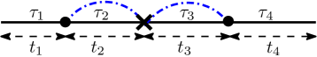
Figure 25: An illustration for a change of variables in the amplitude Eq. (400) of the diagram $D$ in Fig. 21 to write the expression in Eq. (402). Inside each time window $t_{i}$ the process is conditioned to stay a net $\tau_{i}$ amount of time on positive side.

Among the two diagrams in Fig. 21 which contribute to second order, the diagram $D$ is simpler to evaluate. Corresponding amplitude is in Eq. (219), which can be expressed in terms of conditional propagator Eq. (196) using the correlation in Eq. (207).

$$D(\tau, T)=\frac{2^{2}D^{2}}{2D}\int_{0}^{\Lambda}dy_{1}dy_{2}\int_{0}^{T}dr_{1}\int_{r_{1}}^{T}ds\int_{s}^{T}dr_{2}$$

$$\times \int\limits_{0}^{r_{1}}d\tau_{1}\int\limits_{0}^{r_{2}-r_{1}}d\tau_{2}\int\limits_{0}^{T-r_{2}}d\tau_{3}\int\limits_{-\infty}^{\infty}dx_{1}\,dx_{2}\,dm$$

$$\times \delta(\tau-\tau_{1}-\tau_{2}-\tau_{3})\,e^{y_{1}(r_{1}-s)}e^{y_{2}(s-r_{2})}\,\mathbb{Z}_{r_{1}}(0,x_{1}|\tau_{1})$$

$$\times \partial_{x_{1}}\mathbb{Z}_{r_{2}-r_{1}}(x_{1},x_{2}|\tau_{2})\,\partial_{x_{2}}\mathbb{Z}_{T-r_{2}}(x_{2},m|\tau_{3}).$$ (400)

For reasons that will be clear shortly, we make a change of variables (see illustration in Fig. 25), and write

$$D(\tau,T) =2D\int_{0}^{\Lambda}dy_{1}dy_{2}\int_{0}^{\infty}dt_{1}dt_{2}dt_{3}dt_{4}$$ (401)

$$\times\int_{0}^{t_{1}} d\tau_{1}\int_{0}^{t_{2}}d\tau_{2}\int_{0}^{t_{3}}d\tau_{3}\int_{0}^{t_{4}}d\tau_{4}\int_{-\infty}^{\infty}dx_{1}dx_{2}dx_{3}dm$$

$$\times \delta(T-t_{1}-t_{2}-t_{3}-t_{4})\;\delta(\tau-\tau_{1}-\tau_{2}-\tau_{3}-\tau_{4})$$

$$\times e^{-y_{1}t_{2}-y_{2}t_{3}}\;\mathbb{Z}_{t_{1}}(0,x_{1}|\tau_{1})\;\partial_{x_{1}}\mathbb{Z}_{t_{2}}(x_{1},x_{2}|\tau_{2})$$

$$\times \mathbb{Z}_{t_{3}}(x_{2},x_{3}|\tau_{3})\;\partial_{x_{3}}\mathbb{Z}_{t_{4}}(x_{3},m|\tau_{4}),$$ (402)

where in the last two lines of the expression we used $\mathbb{Z}_{t_{2}+t_{3}}(x_{1},x_{3}|\tau_{2}+\tau_{3})=\int dx_{2}\mathbb{Z}_{t_{2}}(x_{1},x_{2}|\tau_{2})\mathbb{Z}_{t_{3}}(x_{2},x_{3}|\tau_{3})$.

A double Laplace transformation Eq. (77) of the amplitude gives a simpler expression

$$\widetilde{D}(\lambda,s)= 2D\int_{0}^{\Lambda}dy_{1}dy_{2}\int_{-\infty}^{\infty}dx_{1}dx_{2}dx_{3}dm\;\widetilde{\mathbb{Z}}_{s}(0,x_{1}|\lambda)$$

$$\times\partial_{x_{1}} \widetilde{\mathbb{Z}}_{s+y_{1}}(x_{1},x_{2}|\lambda)\;\widetilde{\mathbb{Z}}_{s+y_{2}}(x_{2},x_{3}|\lambda)\;\partial_{x_{3}}\widetilde{\mathbb{Z}}_{s}(x_{3},m|\lambda)$$

with $\widetilde{\mathbb{Z}}$ defined in Eq. (204).

Results for spatial integration of $\widetilde{\mathbb{Z}}_{s}$ are derived in App. P and successively using them we get (a lengthy but straightforward algebra) an explicit expression for the amplitude.

$$\widetilde{D}(\lambda,s) =\frac{2}{\sqrt{s(s+\lambda)}\left(\sqrt{s}+\sqrt{s+\lambda}\right)}\int_{0}^{\Lambda}\frac{dy_{1}dy_{2}}{y_{1}y_{2}}$$

$$\qquad\times\left\{\frac{y_{2}\,\mathfrak{h}(1,z,y_{1})}{(y_{2}-y_{1})}+\frac{y_{1}\,\mathfrak{h}(1,z,y_{2})}{(y_{1}-y_{2})}\right\},$$ (403)

where $\mathfrak{h}(s_{1},s_{2},y)$ is defined in Eq. (222). In terms of re-scaled variables, Eq. (403) gives Eq. (220).

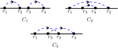
Figure 26: The diagram $C$ in Fig. 21 is split into three parts according to relative position of the loops. For these diagrams we choose $r_{2}>r_{1}$ and $r_{4}>r_{3}$, as indicated by the arrowheads.

For the diagram $C$ in Fig. 21, we write the amplitude (217) in three parts according to the order of time variables (associated diagrams are indicated in Fig. 26). For example, amplitude of diagram $C_{1}$ is

$$C_{1}(\tau,T)= \frac{2}{8D^{2}}\int_{-\infty}^{\infty}dm\int_{0}^{\Lambda}dy_{1}dy_{2}\int_{0}^{T}dr_{1}$$

$$\times \int_{r_{1}}^{T}dr_{2}\int_{r_{2}}^{T}dr_{3}\int_{r_{3}}^{T}dr_{4}\;e^{y_{1}(r_{1}-r_{2})}e^{y_{2}(r_{3}-r_{4})}$$

$$\times\mathopen{\hbox{${\big{\langle}}$}\kern-2.72221pt\leavevmode\hbox{${\big{\langle}}$}}\dot{x}(r_{1})\dot{x}(r_{2})\dot{x}(r_{3})\dot{x}(r_{4})\mathclose{\hbox{${\big{\rangle}}$}\kern-2.72221pt\leavevmode\hbox{${\big{\rangle}}$}}_{(0,m)},$$ (404)

where the pre-factor $2$ is the degeneracy for exchange of pairs $(r_{1},r_{2})$ and $(r_{3},r_{4})$ for the diagram $C_{1}$ in Fig. 26.

Similar to the diagram $D$, these amplitudes can be expressed in terms of conditional propagator (196). The four point correlation in the conditional case is given by, for $r_{1}<r_{2}<r_{3}<r_{4}<T$,

$$\mathopen{\hbox{${\langle}$}\kern-2.72221pt\leavevmode\hbox{${\langle}$}}\dot{x}(r_{1})\dot{x}(r_{2})\dot{x}(r_{3})\dot{x}(r_{4})\mathclose{\hbox{${\rangle}$}\kern-2.72221pt\leavevmode\hbox{${\rangle}$}}_{(m_{1},m_{2})}=2^{4}D^{4}\int_{-\infty}^{\infty}dx_{1}dx_{2}\times$$ (405)

$$dx_{3}dx_{4}\int_{0}^{r_{1}}d\tau_{1}\int_{0}^{r_{2}-r_{1}}d\tau_{2}\int_{0}^{r_{3}-r_{2}}d\tau_{3}\int_{0}^{r_{4}-r_{3}}d\tau_{4}\int_{0}^{T-r_{4}}d\tau_{5}$$

$$\qquad\times\delta(\tau-\tau_{1}-\tau_{2}-\tau_{3}-\tau_{4}-\tau_{5})\mathbb{Z}_{r_{1}}(m_{1},x_{1}|\tau_{1})$$

$$\qquad\times\partial_{x_{1}}\mathbb{Z}_{r_{2}-r_{1}}(x_{1},x_{2}|\tau_{2})\partial_{x_{2}}\mathbb{Z}_{r_{3}-r_{2}}(x_{2},x_{3}|\tau_{3})$$

$$\qquad\times\partial_{x_{3}}\mathbb{Z}_{r_{4}-r_{3}}(x_{3},x_{4}|\tau_{4})\partial_{x_{4}}\mathbb{Z}_{T-r_{4}}(x_{4},m_{2}|\tau_{5}),$$ (406)

where the conditional average is defined in Eq. (195). This is analogous to Eq. (447) without a condition on positive time and can be derived following a similar analysis given in Sec. M.

Following this result (406) and the amplitude in Eq. (404) we write the

$$C_{1}(\tau,T) =2\times\frac{2^{4}D^{4}}{8D^{2}}\int_{0}^{\Lambda}dy_{1}dy_{2}\int_{0}^{\infty}dt_{1}dt_{2}dt_{3}dt_{4}dt_{5}$$

$$\times\int_{0}^{t_{1}}d\tau_{1}\int_{0}^{t_{2}}d\tau_{2}\int_{0}^{t_{3}}d\tau_{3}\int_{0}^{t_{4}}d\tau_{4}\int_{0}^{t_{5}}d\tau_{5}$$

$$\times\int_{-\infty}^{\infty} dx_{1}dx_{2}dx_{3}dx_{4}dm\;\delta(T-t_{1}-t_{2}-t_{3}-t_{4}-t_{5})$$

$$\times\delta(\tau-\tau_{1}-\tau_{2}-\tau_{3}-\tau_{4}-\tau_{5})\;e^{-y_{1}t_{2}-y_{2}t_{4}}$$

$$\times\mathbb{Z}_{t_{1}}( 0,x_{1}|\tau_{1})\partial_{x_{1}}\mathbb{Z}_{t_{2}}(x_{1},x_{2}|\tau_{2})\partial_{x_{2}}\mathbb{Z}_{t_{3}}(x_{2},x_{3}|\tau_{3})$$

$$\times\partial_{x_{3}}\mathbb{Z}_{t_{4}}(x_{3},x_{4}|\tau_{4})\partial_{x_{4}}\mathbb{Z}_{t_{4}}(x_{4},m|\tau_{4}),$$ (407)

where we have made a change of integration variables similar to that used for the diagram $D$ in Eq. (402).

Following a very similar analysis we find that amplitude of other two diagrams in Fig. 26 are almost same as in Eq. (407), with only the term $e^{-y_{1}r_{2}-y_{2}r_{4}}$ replaced by $e^{-y_{1}(t_{2}+t_{3}+t_{4})-y_{2}t_{3}}$ for $C_{2}$ and by $e^{-y_{1}(t_{2}+t_{3})-y_{2}(t_{3}+t_{4})}$ for $C_{3}$.

A double Laplace transformation (77) of the amplitudes integrates the delta functions and lead to a simpler formula,

$$\widetilde{C}_{1}(\lambda,s)= 4D^{2}\int_{0}^{\Lambda}dy_{1}dy_{2}\int_{-\infty}^{\infty}dx_{1}dx_{2}dx_{3}dx_{4}dm$$

$$\times\widetilde{\mathbb{Z}}_{s} (0,x_{1}|\lambda)\partial_{x_{1}}\widetilde{\mathbb{Z}}_{s+y_{1}}(x_{1},x_{2}|\lambda)\partial_{x_{2}}\widetilde{\mathbb{Z}}_{s}(x_{2},x_{3}|\lambda)$$

$$\times\partial_{x_{3}}\widetilde{\mathbb{Z}}_{s+y_{2}}(x_{3},x_{4}|\lambda)\partial_{x_{4}}\widetilde{\mathbb{Z}}_{s}(x_{4},m|\lambda),$$ (408)

with $\widetilde{\mathbb{Z}}$ defined in Eq. (204). The other two amplitudes

$$\widetilde{C}_{2}(\lambda,s)= 4D^{2}\int_{0}^{\Lambda}dy_{1}dy_{2}\int_{-\infty}^{\infty}dx_{1}dx_{2}dx_{3}dx_{4}dm$$

$$\widetilde{\mathbb{Z}}_{s}(0,x_{1} \lambda)\partial_{x_{1}}\widetilde{\mathbb{Z}}_{s+y_{1}}(x_{1},x_{2}|\lambda)\partial_{x_{2}}\widetilde{\mathbb{Z}}_{s+y_{1}+y_{2}}(x_{2},x_{3}|\lambda)$$

$$\partial_{x_{3}}\widetilde{\mathbb{Z}}_{s+y_{1}}(x_{3},x_{4}|\lambda)\partial_{x_{4}}\widetilde{\mathbb{Z}}_{s}(x_{4},m|\lambda),$$ (409)

and

$$\widetilde{C}_{3} (\lambda,s)=4D^{2}\int_{0}^{\Lambda}dy_{1}dy_{2}\int_{-\infty}^{\infty}dx_{1}dx_{2}dx_{3}dx_{4}dm$$

$$\widetilde{\mathbb{Z}}_{s}(0,x_{1}|\lambda)\partial_{x_{1}}\widetilde{\mathbb{Z}}_{s+y_{1}}(x_{1},x_{2}|\lambda)\partial_{x_{2}}\widetilde{\mathbb{Z}}_{s+y_{1}+y_{2}}(x_{2},x_{3}|\lambda)$$

$$\qquad\qquad\partial_{x_{3}}\widetilde{\mathbb{Z}}_{s+y_{2}}(x_{3},x_{4}|\lambda)\partial_{x_{4}}\widetilde{\mathbb{Z}}_{s}(x_{4},m|\lambda).$$ (410)

Difference in Eqs. (409) and (410) are in the subscript of a single $\widetilde{\mathbb{Z}}$ term.

Spatial integrals in these amplitudes can be evaluated by successively applying results from Appendix P. It follows a lengthy but straightforward algebra. We write their final expression as follows.

$$\widetilde{C}_{1}(\lambda,s)=\frac{4}{\sqrt{s(s+\lambda)}\;(\sqrt{s}+\sqrt{s+\lambda})}$$ (411)

$$\times\int_{0}^{\Lambda}\frac{dy_{1}dy_{2}}{y_{1}y_{2}}\bigg{[}\mathfrak{f}(s,s+\lambda,y_{1},y_{2})+\mathfrak{f}(s+\lambda,s,y_{1},y_{2})\bigg{]}$$

with $\mathfrak{f}$ in Eq. (233). Amplitudes of $C_{2}$ and $C_{3}$ are similar,

$$\widetilde{C}_{2}(\lambda,s)+\widetilde{C}_{3}(\lambda,s)=\frac{4}{\sqrt{s(s+\lambda)}\;(\sqrt{s}+\sqrt{s+\lambda})}$$

$$\times\int_{0}^{\Lambda}\frac{dy_{1}dy_{2}}{y_{1}^{2}y_{2}}\bigg{[}\mathfrak{g}(s,s+\lambda,y_{1},y_{2})+\mathfrak{g}(s+\lambda,s,y_{1},y_{2})\bigg{]},$$

with $\mathfrak{g}$ in Eq. (230). Writing them together in terms of re-scaled variables we get Eq. (172).

• We have verified the expression in Eqs. (403), (411), and (J) using the formula Eq. (204) in Eqs. (408), (409), and (410) and then numerically integrating in Mathematica.

Appendix K Expression for $\Psi^{\rm pos}$

Similar to the Eq. (384) for $t_{\rm max}$ we write $\Psi^{\rm pos}$ in Eq. (243) as a combination of three term.

$$\Psi^{\rm pos}\left(y_{1},y_{2},z\right) =\mathfrak{c}+\mathfrak{d}-\frac{1}{4}\mathfrak{a},$$ (413)

where the terms on the right hand side corresponds to amplitudes in Eq. (242). Expression for $\mathfrak{c}(y_{1},y_{2},z)$ is cumbersome to write here and it is given in the supplemental Mathematica notebook [76]. In comparison, $\mathfrak{d}$ and $\mathfrak{a}$ have simpler expression, given below. Their numerical verification is also given in the Mathematica notebook.

$$\mathfrak{d}(y_{1},y_{2},z)= y_{1}y_{2}+\frac{y_{2}^{2}\;r(y_{1},z)-y_{1}^{2}\;r(y_{2},z)}{y_{1}-y_{2}},$$ (414)

with

$$r(y,z)=-\sqrt{z(z-y)}\;\Theta(z-y)+$$ (415)

$$\left(\sqrt{y+1}-1\right)\sqrt{y-z}\;\Theta(y-z)+\sqrt{y+1}+z-1.$$

Here $\Theta(x)$ is the Heaviside step function.

$$\mathfrak{a}(y_{1},y_{2},z)=u(y_{1},y_{2},z)+u(y_{2},y_{1},z),$$ (416)

with

$$u(y_{1},y_{2}, z)=2-4z+\frac{z^{2}}{2}+\frac{y_{1}y_{2}}{2}-y_{1}z+2y_{1}+\bigg{(}6z-4-2y_{2}+2(1-z)\sqrt{y_{2}+1}\bigg{)}\sqrt{y_{1}+1}\;+$$ (417)

$$|y_{1}-z|\bigg{(}\Theta(y_{1}-z)-\Theta(z-y_{1})\bigg{)}\bigg{(}2+y_{2}-z-2\sqrt{y_{2}+1}-2\sqrt{y_{2}+1}\sqrt{y_{2}-z}\;\Theta(y_{2}-z)\bigg{)}+$$ (418)

$$2\sqrt{|y_{2}-z|}\bigg{\{}\Theta(y_{2}-z)\bigg{[}z\left(2\sqrt{y_{1}+1}+\sqrt{y_{2}+1}-3\right)+y_{1}\left(1-\sqrt{y_{2}+1}\right)+$$ (419)

$$\qquad\qquad\qquad\qquad\qquad\qquad 2\left(1-\sqrt{y_{1}+1}-\sqrt{y_{2}+1}+\sqrt{(y_{1}+1)(y_{2}+1)}\right)\bigg{]}+$$ (420)

$$\qquad\qquad\qquad\qquad\quad\sqrt{z}\;\Theta(z-y_{2})\left(2\sqrt{(y_{1}+1)(y_{2}+1)}-4\sqrt{y_{1}+1}-2\sqrt{y_{2}+1}+y_{1}-z+4\right)\bigg{\}}+$$ (421)

$$2|y_{1}-z|\sqrt{|y_{2}-z|}\bigg{(}\Theta(y_{1}-z)-\Theta(z-y_{1})\bigg{)}\bigg{(}\Theta(y_{2}-z)+\sqrt{z}\;\Theta(z-y_{2})\bigg{)}+$$ (422)

$$\frac{1}{2}|y_{1}-z||y_{2}-z|\bigg{(}\Theta(y_{1}-z)-\Theta(z-y_{1})\bigg{)}\bigg{(}\Theta(y_{2}-z)-\Theta(z-y_{2})\bigg{)}-$$ (423)

$$2\sqrt{|y_{1}-z|}\sqrt{|y_{2}-z|}\bigg{\{}\sqrt{z}\left(\sqrt{y_{1}+1}+\sqrt{y_{2}+1}-2\right)\bigg{(}\Theta(y_{1}-z)\Theta(z-y_{2})+\Theta(z-y_{1})\Theta(y_{2}-z)\bigg{)}+$$ (424)

$$\left(z-1+\sqrt{y_{1}+1}+\sqrt{y_{2}+1}-\sqrt{(y_{1}+1)(y_{2}+1)}\right)\bigg{(}\Theta(y_{1}-z)\Theta(y_{2}-z)-\Theta(z-y_{1})\Theta(z-y_{2})\bigg{)}\bigg{\}}.$$ (425)

Appendix L A list of integrals for the Brownian propagator

The Brownian propagator $Z_{t}(m_{1},m_{2})$ in Eq. (25) is symmetric under exchange of $m_{1}$ and $m_{2}$, and therefore

$$\partial_{m_{1}}Z_{t}(m_{1},m_{2})=-\partial_{m_{2}}Z_{t}(m_{1},m_{2})$$ (426)

and its Laplace transformation (102)

$$\partial_{m_{1}}\widetilde{Z}_{s}(m_{1},m_{2})=-\partial_{m_{2}}\widetilde{Z}_{s}(m_{1},m_{2}).$$ (427)

There is an analogous formula for the propagator $\widetilde{Z}^{+}_{s}$ in presence of absorbing line.

$$\partial_{m_{1}}\widetilde{Z}^{+}_{s}(m_{1},m_{2})=-\partial_{m_{2}}\widetilde{Z}^{+}_{s}(m_{1},m_{2})+\frac{1}{D}e^{-\sqrt{\frac{s}{D}}(m_{1}+m_{2})}.$$ (428)

We list the following results for the integral of the propagators, which are frequently used in this paper. They can be numerically verified in Mathematica.

$$\int_{-\infty}^{\infty}dm_{2}\widetilde{Z}_{s}(m_{1},m_{2})=\frac{1}{s}$$ (429)

and its analogue with absorbing boundary

$$\int_{0}^{\infty}dm_{2}\widetilde{Z}^{+}_{s}(m_{1},m_{2})=\frac{1}{s}\left(1-e^{-m_{1}\sqrt{\frac{s}{D}}}\right).$$ (430)

Another useful result

$$\int_{0}^{\infty}dm_{2} \widetilde{Z}^{+}_{s+y}(m_{1},m_{2})e^{-m_{2}\sqrt{\frac{s}{D}}}$$ (431)

$$=\frac{1}{y}\left(e^{-m_{1}\sqrt{\frac{s}{D}}}-e^{-m_{1}\sqrt{\frac{s+y}{D}}}\right).$$ (432)

Due to a symmetry $\widetilde{Z}_{s}(m_{1},m_{2})=\widetilde{Z}_{s}(m_{2},m_{1})$ an integral over $m_{1}$ yields the same results as above.

For product of two propagators we get

$$\int_{-\infty}^{\infty}dx \widetilde{Z}_{r}(m_{1},x)\widetilde{Z}_{s}(x,m_{2})=$$ (433)

$$\begin{cases}\frac{\widetilde{Z}_{s}(m_{1},m_{2})}{r-s}+\frac{\widetilde{Z}_{r}(m_{1},m_{2})}{s-r}&\mbox{if }s\neq r,\\[5.69054pt] \frac{1+\sqrt{\frac{s}{D}}|m_{1}-m_{2}|}{2s}\;\widetilde{Z}_{s}(m_{1},m_{2})&\mbox{if }r=s.\end{cases}$$

and for its analogue with absorbing boundary

$$\int_{0}^{\infty}dx \widetilde{Z}^{+}_{r}(m_{1},x)\widetilde{Z}^{+}_{s}(x,m_{2})=$$ (434)

$$\begin{cases}\displaystyle\frac{\widetilde{Z}^{+}_{s}(m_{1},m_{2})}{r-s}+\frac{\widetilde{Z}^{+}_{r}(m_{1},m_{2})}{s-r}&\mbox{if }s\neq r,\cr&\cr\displaystyle\frac{1+\sqrt{\frac{s}{D}}|m_{1}-m_{2}|}{2s}\;\widetilde{Z}^{+}_{s}(m_{1},m_{2})&\mbox{if }r=s,\\[5.69054pt] \displaystyle\quad-\frac{\min\{m_{1},m_{2}\}}{2s}e^{-(m_{1}+m_{2})\sqrt{\frac{s}{D}}}\end{cases}$$

For product of three propagators, corresponding formula is

$$\int_{-\infty}^{\infty}dx\int_{-\infty}^{\infty}dy\widetilde{Z}_{r}(m_{1},x)\widetilde{Z}_{s}(x,y)\widetilde{Z}_{t}(y,m_{2})=\begin{cases}\displaystyle\frac{\widetilde{Z}_{r}(m_{1},m_{2})}{(s-r)(t-r)}+\frac{\widetilde{Z}_{s}(m_{1},m_{2})}{(r-s)(t-s)}+\frac{\widetilde{Z}_{t}(m_{1},m_{2})}{(r-t)(s-t)}&\mbox{if}\quad r\neq s\neq t\cr&\cr\cr\displaystyle\left[\frac{1+\sqrt{\frac{r}{D}}|m_{1}-m_{2}|}{2r}-\frac{1}{s-r}\right]\frac{\widetilde{Z}_{r}(m_{1},m_{2})}{s-r}\cr\displaystyle\qquad\qquad+\frac{\widetilde{Z}_{s}(m_{1},m_{2})}{(r-s)^{2}}&\mbox{if}\quad r=t\neq s\cr\cr&\cr\displaystyle\left[\frac{1+\sqrt{\frac{r}{D}}|m_{1}-m_{2}|}{2r}-\frac{1}{t-r}\right]\frac{\widetilde{Z}_{r}(m_{1},m_{2})}{t-r}\cr\displaystyle\qquad\qquad+\frac{\widetilde{Z}_{t}(m_{1},m_{2})}{(r-t)^{2}}&\mbox{if}\quad r=s\neq t\end{cases}$$ (435)

and its counterpart in presence of absorbing line,

$$\int_{0}^{\infty}\!\!\!\!dx\int_{0}^{\infty}\!\!\!\!dy\widetilde{Z}^{+}_{r}(m_{1},x)\widetilde{Z}^{+}_{s}(x,y)\widetilde{Z}^{+}_{t}(y,m_{2})=\begin{cases}\displaystyle\frac{\widetilde{Z}^{+}_{r}(m_{1},m_{2})}{(s-r)(t-r)}+\frac{\widetilde{Z}^{+}_{s}(m_{1},m_{2})}{(r-s)(t-s)}+\frac{\widetilde{Z}^{+}_{t}(m_{1},m_{2})}{(r-t)(s-t)}&\mbox{if}\quad r\neq s\neq t\cr\cr\cr\displaystyle\left[\frac{1+\sqrt{\frac{r}{D}}|m_{1}-m_{2}|}{2r}-\frac{1}{s-r}\right]\frac{\widetilde{Z}^{+}_{r}(m_{1},m_{2})}{s-r}\cr\displaystyle\quad+\frac{\widetilde{Z}^{+}_{s}(m_{1},m_{2})}{(r-s)^{2}}-\frac{\min(m_{1},m_{2})}{2r(s-r)}e^{-(m_{1}+m_{2})\sqrt{\frac{r}{D}}}&\mbox{if}\quad r=t\neq s\cr\cr\cr\displaystyle\left[\frac{1+\sqrt{\frac{r}{D}}|m_{1}-m_{2}|}{2r}-\frac{1}{t-r}\right]\frac{\widetilde{Z}^{+}_{r}(m_{1},m_{2})}{t-r}\cr\displaystyle\quad+\frac{\widetilde{Z}^{+}_{t}(m_{1},m_{2})}{(r-t)^{2}}-\frac{\min(m_{1},m_{2})}{2r(t-r)}e^{-(m_{1}+m_{2})\sqrt{\frac{r}{D}}}&\mbox{if}\quad r=s\neq t\end{cases}$$ (436)

Appendix M Time-correlation of Brownian velocities

Here, we derive multi-time correlations of velocity $\dot{x}(t)$ for a standard Brownian motion with diffusivity $D$. The first moment is defined by

$$\langle\dot{x}(t)\rangle=\int_{x(0)=m_{1}}^{x(T)=m_{2}}\mathcal{D}[x]e^{-\frac{S_{0}}{D}}\dot{x}(t),$$ (437)

where the angular brackets denote average with a Brownian measure of diffusivity $D$ starting at position $x(0)=m_{1}$ and finishing at time $T$ at position $x(T)=m_{2}$. For evaluating the average we consider a small window between time $t$ and $t+\Delta t$ such that

$$\langle\dot{x}(t) \rangle=\lim_{\Delta t\to 0}\int_{-\infty}^{\infty}dxdy\;Z_{t}(m_{1},x)\times$$ (438)

$$\left[\frac{e^{-\frac{(y-x)^{2}}{4D\Delta t}}}{\sqrt{4\pi D\Delta t}}\left(\frac{y-x}{\Delta t}\right)\right]Z_{T-t-\Delta t}(y,m_{2}),$$ (439)

where the Brownian propagator $Z$ is in Eq. (25) and we use Eq. (8a) for small $\Delta t$. Writing

$$\frac{e^{-\frac{(y-x)^{2}}{4D\Delta t}}}{\sqrt{4\pi D\Delta t}}\left(\frac{y-x}{\Delta t}\right)=-2D\;\partial_{y}\left[\frac{e^{-\frac{(y-x)^{2}}{4D\Delta t}}}{\sqrt{4\pi D\Delta t}}\right]$$

and using integration by parts for $y$ variable, we get

$$\langle\dot{x}(t) \rangle=2D\int_{-\infty}^{\infty}dxdy\;Z_{t}(m_{1},x)\times$$

$$\lim_{\Delta t\to 0}\left[\frac{e^{-\frac{(y-x)^{2}}{4D\Delta t}}}{\sqrt{4\pi D\Delta t}}\right]\partial_{y}Z_{T-t-\Delta t}(y,m_{2}).$$

In the $\Delta t\to 0$ limit, it gives an expression

$$\langle\dot{x}(t)\rangle=2D\int_{-\infty}^{\infty}dx\;Z_{t}(m_{1},x)\partial_{x}\;Z_{T-t}(x,m_{2}),$$ (440)

which can be explicitly evaluated using Eq. (25).

For two-time correlation one can similarly show that

$$\langle\dot{x}(r_{1})\dot{x}(r_{2})\rangle= 2^{2}D^{2}\mathscr{C}(r_{1},r_{2})$$ (441)

$$+2D\;\delta(r_{1}-r_{2})Z_{T}(m_{1},m_{2}),$$ (442)

where $\mathscr{C}(r_{1},r_{2})$ is a symmetric function given by

$$\mathscr{C}(r_{1},r_{2}) =\int_{-\infty}^{\infty}dx_{1}dx_{2}Z_{r_{1}}(m_{1},x_{1})\times$$ (443)

$$\partial_{x1}Z_{r_{2}-r_{1}}(x_{1},x_{2})\partial_{x2}Z_{T-r_{2}}(x_{2},m_{2}),$$ (444)

for $r_{2}>r_{1}$. The integral remains finite for $r_{1}\to r_{2}$ limit.

A generalization of Eq. (442) in an analogy of Wick’s theorem gives multi-time correlations. For example, we get

$$\langle \dot{x}(r_{1})\dot{x}(r_{2})\dot{x}(r_{3})\rangle=$$ (445)

$$\qquad 2^{3}D^{3}\mathscr{C}(r_{1},r_{2},r_{3})+2D\sum_{\text{p}airs}\delta(r_{i}-r_{j})\langle\dot{x}(r_{k})\rangle,$$

where $\mathscr{C}(r_{1},r_{2},r_{3})$ is a symmetric function under permutation of its arguments and given by

$$\mathscr{C}(r_{1},r_{2},r_{3})= \int_{-\infty}^{\infty}dx_{1}dx_{2}dx_{3}Z_{r_{1}}(m_{1},x_{1})$$ (446)

$$\times \partial_{x_{1}}Z_{r_{2}-r_{1}}(x_{1},x_{2})\;\partial_{x_{2}}Z_{r_{3}-r_{2}}(x_{2},x_{3})$$

$$\times \partial_{x_{3}}Z_{T-r_{3}}(x_{3},m_{2}),$$

for $r_{3}>r_{1}>r_{1}$.

For the four-time correlation, we get

$$\langle\dot{x}(r_{1})\dot{x}(r_{2})\dot{x}(r_{3}) \dot{x}(r_{4})\rangle=2^{4}D^{4}\mathscr{C}(r_{1},r_{2},r_{3},r_{4})$$

$$+2D\sum_{pairs}\delta(r_{i}-r_{j})\langle\dot{x}(r_{k})\dot{x}(r_{\ell})\rangle$$ (447)

with

$$\mathscr{C}(r_{1},r_{2},r_{3},r_{4})= \int_{-\infty}^{\infty}dx_{1}dx_{2}dx_{3}dx_{4}\times$$ (448)

$$Z_{r_{1}}(m_{1},x_{1}) \partial_{x_{1}}Z_{r_{2}-r_{1}}(x_{1},x_{2})\partial_{x_{2}}Z_{r_{3}-r_{2}}(x_{2},x_{3})$$

$$\times\partial_{x_{3}} Z_{r_{4}-r_{3}}(x_{3},x_{4})\partial_{x_{4}}Z_{T-r_{4}}(x_{4},m_{2}),$$

for $r_{1}<r_{2}<r_{3}<\cdots<r_{4}$.

Expression for these correlations can be further simplified. For the first moment Eq. (440), using Eq. (426) and then integrating over $x$, we get

$$\langle\dot{x}(t)\rangle=(-2D\partial_{m_{2}})Z_{T}(m_{1},m_{2}).$$ (449)

Similarly, from Eq. (442) we get

$$\langle\dot{x}(r_{1})\dot{x}(r_{2})\rangle=\left[2^{2}D^{2}\partial_{m_{2}}+2D\delta(r_{1}-r_{2})\right]Z_{T}(m_{1},m_{2}),$$ (450)

and for three-time correlation in Eq. (445) we get

$$\langle\dot{x}(r_{1})\dot{x}(r_{2})\dot{x}(r_{3} )\rangle=(-2D\;\partial_{m_{2}})\bigg{[}2^{2}D^{2}\partial_{m_{2}}^{2}+$$ (451)

$$2D\sum_{\text{p}airs}\delta(r_{i}-r_{j})\bigg{]}Z_{T}(m_{1},m_{2}).$$ (452)

More generally, for $r_{1}<r_{2}<\cdots<r_{2n}$ we see that

$$\langle\dot{x}(r_{1})\cdots\dot{x}(r_{2n})\rangle=2^{2n}D^{2n}\partial^{2n}_{m_{2}}Z_{T}(m_{1},m_{2}),$$ (453)

which is used for a derivation of Eq. (261).

• Formulas in Eqs. (450) and (452) are mentioned earlier in Eqs. (26) and (32).

• In presence of an absorbing wall, correlations have a very similar formula as in Eqs. (440), (442), (445), and (447), where one need to substitute the propagator $Z$ by $Z^{+}$. However, they can not be simplified like in Eqs. (449 - 452).

Appendix N Identities for $J_{t}$ in Eq. (107)

In this section, we give a list of results for $J_{t}$ in Eq. (107) and its analogue $J_{t}^{+}$ with absorbing boundary. These results are used in our analysis.

N.1 $J_{t}(m_{1},m_{2};y)$

Using (449) in Eq. (107) we write

$$J_{t}(m_{1},m_{2};y)=2D\;\partial_{m_{2}}Z_{t}(m_{1},m_{2})\left\{\frac{e^{-yt}-1}{y}\right\}.$$

It’s Laplace transform is

$$\widetilde{J}_{s}(m_{1},m_{2};y)=\frac{2D}{y}\partial_{m_{2}}\left(\widetilde{Z}_{s+y}(m_{1},m_{2})-\widetilde{Z}_{s}(m_{1},m_{2})\right)$$

and using Eq. (102a) it leads to

$$\widetilde{J}_{s}(m_{1},m_{2} ;y)=\frac{{\mathrm{sgn}}(m_{1}-m_{2})}{y}\times$$ (454)

$$\left[e^{-|m_{1}-m_{2}|\sqrt{\frac{s+y}{D}}}-e^{-|m_{1}-m_{2}|\sqrt{\frac{s}{D}}}\right].$$ (455)

Here ${\mathrm{sgn}}(x)$ gives the sign of $x$.

N.2 $J_{t}^{+}(m_{1},m_{2};y)$

An analogue of $J_{t}$ in presence of absorbing line is

$$J_{t}^{+}(m_{1},m_{2};y)=\int_{0}^{t}dr\;e^{-yr}\langle\dot{x}(r)\rangle^{+},$$ (456)

with the average $\langle\cdot\rangle^{+}$ defined as in Eq. (437) with absorbing boundary at origin. Using the analogous formula of Eq. (440) for absorbing boundary and taking Laplace transformation we get

$$\widetilde{J}_{s}^{+}(m_{1},m_{2};y)=2D\int_{0}^{\infty}dx\widetilde{Z}_{s+y}^{+}(m_{1},x)\partial_{x}\widetilde{Z}_{s}^{+}(x,m_{2}).$$ (457)

Further, using Eq. (428) and Eq. (434) leads

$$\widetilde{J}^{+}_{s}(m_{1},m_{2};y)=-2D\partial_{m_{2}}\Bigg{[}\int_{0}^{\infty}dx\widetilde{Z}^{+}_{s+y}(m_{1},x)\times$$ (458)

$$\widetilde{Z}^{+}_{s}(x,m_{2})\Bigg{]}+2\int_{0}^{\infty}dx\widetilde{Z}^{+}_{s+y}(m_{1},x)e^{-\sqrt{\frac{s}{D}}(x+m_{2})}.$$ (459)

Invoking the explicit expression of $\widetilde{Z}^{+}$ in Eq. (102b) leads to a small $x_{0}$ asymptotic,

$$\widetilde{J}^{+}_{s}(m_{1},x_{0};y)\simeq\frac{2x_{0}\sqrt{s}}{y\sqrt{D}}\left\{e^{-m_{1}\sqrt{\frac{s+y}{D}}}-e^{-m_{1}\sqrt{\frac{s}{D}}}\right\},$$ (460)

which has been used many times in our analysis.

Another useful result is for integrals of $\widetilde{J}^{+}_{s}$. It is straightforward to see that an integration over $m_{1}$ gives

$$\int_{0}^{\infty} dm_{1}\widetilde{J}^{+}_{s}(m_{1},m_{2};y)$$ (461)

$$=\frac{2\sqrt{D}}{y\sqrt{(s+y)}}\left\{e^{-m_{2}\sqrt{\frac{s+y}{D}}}-e^{-m_{2}\sqrt{\frac{s}{D}}}\right\},$$ (462)

and an integration over $m_{2}$ gives

$$\int_{0}^{\infty}dm_{2} \widetilde{J}^{+}_{s}(m_{1},m_{2};y)$$ (463)

$$=\frac{2\sqrt{D}}{y\sqrt{s}}\left\{e^{-m_{1}\sqrt{\frac{s}{D}}}-e^{-m_{1}\sqrt{\frac{s+y}{D}}}\right\},$$ (464)

where we used Eq. (432). The same result can also be derived using a symmetry

$$\widetilde{J}^{+}_{s}(m_{1},m_{2};y)=-\widetilde{J}^{+}_{s+y}(m_{2},m_{1};-y),$$

which is evident from Eq. (459) and the symmetry of $\widetilde{Z}^{+}_{t}$.

N.3 $J_{t}(m_{1},m_{2};y_{1},y_{2})$

For $J_{t}(m_{1},m_{2};y_{1},y_{2})$ in Eq. (107) using the correlation Eq. (450) with the choice of integration Eq. (15) we get

$$J_{t}(m_{1},m_{2};y_{1},y_{2})$$

$$=2^{2}D^{2}\frac{\partial^{2}_{m_{2}}Z_{t}(m_{1},m_{2})}{y_{1}y_{2}}\left[\frac{y_{1}+y_{2}e^{-t(y_{1}+y_{2})}}{y_{1}+y_{2}}-e^{-y_{2}t}\right].$$

A Laplace transformation gives

$$\widetilde{J}_{s}(m_{1},m_{2};y_{1},y_{2})=\frac{2^{2}D^{2}}{y_{1}y_{2}(y_{1}+y_{2})}\bigg{[}y_{1}\partial^{2}_{m_{2}}\widetilde{Z}_{s}(m_{1},m_{2})+$$

$$y_{2}\partial^{2}_{m_{2}}\widetilde{Z}_{s+y_{1}+y_{2}}(m_{1},m_{2})-(y_{1}+y_{2})\partial^{2}_{m_{2}}\widetilde{Z}_{s+y_{2}}(m_{1},m_{2})\bigg{]}.$$

The explicit formula of $\widetilde{Z}$ in Eq. (102a) leads to the result given in Eq. (297).

A special case of Eq. (297), used earlier for deriving the result Eq. (108), is

$$\widetilde{J}_{s}(0,x_{0};-y ,y)=\frac{\sqrt{D}}{y^{2}}\Bigg{[}2\sqrt{s+y}e^{-x_{0}\sqrt{\frac{s+y}{D}}}$$ (465)

$$-\frac{e^{-x_{0}\sqrt{\frac{s}{D}}}}{\sqrt{s}}\bigg{(}2s+y-yx_{0}\sqrt{\frac{s}{D}}\bigg{)}\,\Bigg{]}.$$ (466)

N.4 $J_{t}^{+}(m_{1},m_{2};y_{1},y_{2})$

Starting with the definition

$$J_{t}^{+} (m_{1},m_{2};y_{1},y_{2})$$ (467)

$$=\int_{0}^{t}dr_{1}\int_{r_{1}}^{t}dr_{2}\;e^{-y_{1}r_{1}-y_{2}r_{2}}\langle\dot{x}(r_{1})\dot{x}(r_{2})\rangle^{+}$$ (468)

with the convention in Eq. (15) for time-integrals and using an analogue of Eq. (442) for correlations with absorbing boundary, we write

$$J_{t}^{+}(m_{1}, m_{2};y_{1},y_{2})=\int_{-\infty}^{\infty}dx_{1}dx_{2}\int_{0}^{t}dr_{1}\int_{r_{1}}^{t}dr_{2}\;e^{-y_{1}r_{1}-y_{2}r_{2}}$$

$$\times Z_{r_{1}}(m_{1},x_{1})\partial_{x1}Z_{r_{2}-r_{1}}(x_{1},x_{2})\partial_{x2}Z_{T-r_{2}}(x_{2},m_{2}).$$

It’s Laplace transformation (in $t\to s$ variable) is

$$\widetilde{J}_{s}^{+} (m_{1},m_{2};y_{1},y_{2})=2^{2}D^{2}\int_{0}^{\infty}dx_{1}dx_{2}\times$$ (469)

$$\widetilde{Z}^{+}_{s+y_{1}+y_{2}}(m_{1},x_{1})\partial_{x_{1}}\widetilde{Z}^{+}_{s+y_{2}}(x_{1},x_{2})\partial_{x_{2}}\widetilde{Z}^{+}_{s}(x_{2},m_{2}).$$

An explicit expression can be derived using the result in (102b).

Analysis gets simplified realizing that

$$\widetilde{J}_{s}^{+} (m_{1},m_{2};y_{1},y_{2})$$ (470)

$$=2D\int_{0}^{\infty}dx\widetilde{Z}^{+}_{s+y_{1}+y_{2}}(m_{1},x)\partial_{x}\widetilde{J}_{s}^{+}(x,m_{2},y_{2}),$$

with $\widetilde{J}_{s}^{+}(x,m_{2},y_{2})$ in Eq. (457). Using this, for example, one can derive a useful asymptotic for small $x_{0}$ by using Eq. (460) and Eq. (102b), which gives

$$\widetilde{J}_{s}^{+} (m_{1},x_{0};y_{1},y_{2})$$ (471)

$$\simeq \;4x_{0}\Bigg{\{}\frac{s}{y_{2}(y_{1}+y_{2})}\left(e^{-m_{1}\sqrt{\frac{s}{D}}}-e^{-m_{1}\sqrt{\frac{s+y_{1}+y_{2}}{D}}}\right)$$ (472)

$$- \frac{\sqrt{s(s+y_{2})}}{y_{1}y_{2}}\left(e^{-m_{1}\sqrt{\frac{s+y_{2}}{D}}}-e^{-m_{1}\sqrt{\frac{s+y_{1}+y_{2}}{D}}}\right)\Bigg{\}}.\qquad$$ (473)

For an analogous formula of Eq. (464) we evaluate the integration in Eq. (470) using Eq. (430), a symmetry $\widetilde{Z}^{+}_{s}(m_{1},m_{2})=\widetilde{Z}^{+}_{s}(m_{2},m_{1})$, the results in Eqs. (427), (432), (434), and using integration by parts. This way it is straightforward to get the result in Eq. (300).

In a similar way we derive the integral over $m_{1}$, and the result is given in Eq. (339). Alternatively, one can use a symmetry

$$\widetilde{J}_{s}^{+}(m_{1},m_{2};y_{1},y_{2})=\widetilde{J}_{s+y_{1}+y_{2}}^{+}(m_{2},m_{1};-y_{2},-y_{1}),$$

which is evident from Eq. (476) using the symmetry $\widetilde{Z}_{s}^{+}(x_{1},x_{2})=\widetilde{Z}_{s}^{+}(x_{2},x_{1})$.

A special case of Eq. (300), which is used for deriving Eq. (108), is

$$\int_{0}^{\infty} dm_{2}\widetilde{J}_{s}^{+}(m_{1},m_{2};-y,y)=\frac{2\sqrt{D}}{y^{2}\sqrt{s}}\bigg{\{}2\sqrt{(s+y)}\times$$ (474)

$$\sqrt{D}\left(e^{-m_{1}\sqrt{\frac{s}{D}}}-e^{-m_{1}\sqrt{\frac{s+y}{D}}}\right)-m_{1}ye^{-m_{1}\sqrt{\frac{s}{D}}}\bigg{\}}.\quad$$ (475)

N.5 $J_{t}^{+}(m_{1},m_{2};y_{1},y_{2},y_{3})$

Similar to Eq. (468) we define $J_{t}^{+}(m_{1},m_{2};y_{1},y_{2},y_{3})$. Using the analogue of Eq. (445) with an absorbing boundary and then taking a Laplace transformation (in $t\to s$ variable) we write

$$\widetilde{J}_{s}^{+}(m_{1},m_{2}; y_{1},y_{2},y_{3})=2^{3}D^{3}\int_{0}^{\infty}dx_{1}dx_{2}dx_{3}$$

$$\times\widetilde{Z}_{s+y_{1}+y_{2}+y_{3}}^{+}(m_{1},x_{1})\partial_{x_{1}}\widetilde{Z}_{s+y_{2}+y_{3}}^{+}(x_{1},x_{2})$$

$$\times\partial_{x_{2}}\widetilde{Z}_{s+y_{3}}^{+}(x_{2},x_{3})\partial_{x_{3}}\widetilde{Z}_{s}^{+}(x_{3},m_{2}).$$ (476)

For an explicit result we note that

$$\widetilde{J}_{s}^{+}(m_{1},m_{2}; y_{1},y_{2},y_{3})=2D\int_{0}^{\infty}dx$$ (477)

$$\times\widetilde{Z}^{+}_{s+y_{1}+y_{2}+y_{3}}(m_{1},x)\partial_{x}\widetilde{J}^{+}_{s}(x,m_{2};y_{2},y_{3})$$

with Eq. (476). Then, Eqs. (102b) and (473) can be used to get an asymptotic for small $x_{0}$.

Integral of $\widetilde{J}_{s}^{+}(m_{1},x_{0};y_{1},y_{2},y_{3})$ analogous to Eq. (462) is also straightforward to derive using Eq. (477). For small $x_{0}$,

$$\int_{0}^{\infty}dm_{1} \widetilde{J}_{s}^{+}(m_{1},x_{0};y_{1},y_{2},y_{3})\simeq 8Dx_{0}$$

$$\bigg{\{} \frac{\left(s+y_{3}\right)\left(\sqrt{s+y_{3}}-\sqrt{s+y_{1}+y_{2}+y_{3}}\right)}{\sqrt{s}\;y_{2}\left(y_{1}+y_{2}\right)y_{3}}+$$

$$\frac{\sqrt{s+y_{2}+y_{3}}\left[\left(y_{2}+y_{3}\right)\sqrt{s+y_{3}}-y_{2}\sqrt{s}\right]}{\sqrt{s}\;y_{1}y_{2}y_{3}\left(y_{2}+y_{3}\right)}\times$$

$$\left(\sqrt{s+y_{1}+y_{2}+y_{3}}-\sqrt{s+y_{2}+y_{3}}\right)+$$

$$\frac{\sqrt{s}\left(\sqrt{s+y_{1}+y_{2}+y_{3}}-\sqrt{s}\right)}{y_{3}\left(y_{2}+y_{3}\right)\left(y_{1}+y_{2}+y_{3}\right)}\bigg{\}},$$ (478)

which is used for a derivation of Eq. (357).

For an integral over $m_{2}$ variable, one can use a symmetry

$$\widetilde{J}_{s}^{+} (m_{1},m_{2};y_{1},y_{2},y_{3})$$ (479)

$$=-\widetilde{J}_{s+y_{1}+y_{2}+y_{3}}^{+}(m_{2},m_{1};-y_{3},-y_{2},-y_{1}),$$ (480)

which is evident from Eq. (476) and $\widetilde{Z}^{+}_{s}(m_{1},m_{2})=\widetilde{Z}^{+}_{s}(m_{2},m_{1})$. The result is useful for a derivation of Eq. (364).

N.6 $J_{t}^{+}(m_{1},m_{2};y_{1},y_{2},y_{3},y_{4})$

Similar to Eqs. (470) and (477),

$$J_{t}^{+}(m_{1}, m_{2};y_{1},y_{2},y_{3},y_{4})=\int_{0}^{t}dr_{1}\int_{r_{1}}^{t}dr_{2}\int_{r_{2}}^{t}dr_{3}\times$$ (481)

$$\int_{r_{3}}^{t}dr_{4} e^{-y_{1}r_{1}-y_{2}r_{2}-y_{3}r_{3}-y_{4}r_{4}}\langle\dot{x}(r_{1})\dot{x}(r_{2})\dot{x}(r_{3})\dot{x}(r_{4})\rangle^{+}$$ (482)

follows a hierarchy where

$$\widetilde{J}_{s}^{+}( m_{1},m_{2};y_{1},y_{2},y_{3},y_{4})=2D\int_{0}^{\infty}dx\times$$ (483)

$$\widetilde{Z}_{s+y_{1}+y_{2}+y_{3}+y_{4}}^{+}(m_{1},x)\;\partial_{x}\widetilde{J}^{+}_{s}(x,m_{2};y_{2},y_{3},y_{4}),\qquad\quad$$ (484)

which leads to explicit results explicit result for Eq. (482).

For example, an integral over $m_{2}$ variable is given in Eq. (305). From this one can derive also the integral over $m_{1}$ variable using a symmetry relation

$$\widetilde{J}_{s}^{+} (m_{1},m_{2};y_{1},y_{2},y_{3},y_{4})$$ (485)

$$= \widetilde{J}_{s+y_{1}+y_{2}+y_{3}+y_{4}}^{+}(m_{2},m_{1};-y_{4},-y_{3},-y_{2},-y_{1}),\qquad$$ (486)

which is evident from Eq. (484) and a symmetry $\widetilde{Z}^{+}_{s}(m_{1},m_{2})=\widetilde{Z}^{+}_{s}(m_{2},m_{1})$.

Appendix O Identities for $\mathscr{I}_{\tau}^{+}$ in Eq. (351)

Using Eq. (352) we get a relation for their Laplace transformation

$$\widetilde{\mathscr{I}}_{s}^{+} (m_{1},m_{2};y_{1},y_{2},y_{3})=\widetilde{J}_{s}^{+}(m_{1},m_{2};y_{1},y_{2},y_{3})$$ (487)

$$\quad+ \widetilde{J}_{s}^{+}(m_{1},m_{2};y_{1},y_{3},y_{2})+\widetilde{J}_{s}^{+}(m_{1},m_{2};y_{3},y_{1},y_{2}).\qquad$$ (488)

This leads to the results we need, namely,

$$\int_{0}^{\infty}dm_{1}\widetilde{\mathscr{I}}_{s+\lambda+y_{2}}^{+} (m_{1},x_{0};-y_{1},y_{1},-y_{2})$$

$$=\int_{0}^{\infty}dm_{1}\bigg{\{} \widetilde{J}_{s+\lambda+y_{2}}^{+}(m_{1},x_{0};-y_{1},y_{1},-y_{2})$$

$$+\widetilde{J}_{s+\lambda+y_{2}}^{+}(m_{1},x_{0};-y_{1},-y_{2},y_{1})$$

$$+\widetilde{J}_{s+\lambda+y_{2}}^{+}(m_{1},x_{0};-y_{2},-y_{1},y_{1})\bigg{\}},$$

which using Eq. (478) for small $x_{0}$ limit gives Eq. (357). A analogous integral

$$\int_{0}^{\infty}dm_{2} \widetilde{\mathscr{I}}_{s}^{+}(x_{0},m_{2};-y_{2},y_{2},y_{1})\simeq\frac{4Dx_{0}\sqrt{s+y_{1}}}{y_{1}y_{2}^{2}\sqrt{s}}\times$$ (489)

$$\bigg{(}\sqrt{s{+}y_{1}{+}y_{2}}-\sqrt{s{+}y_{1}}-\sqrt{s{+}y_{2}}+\sqrt{s}\bigg{)}^{2},$$ (490)

for small $x_{0}$, is derived using Eqs. (488), (478), and (480). It is used for a derivation of Eq. (364).

Appendix P Identities for conditional propagator $\mathbb{Z}_{t}$

In this section we give a list of identities for conditional Brownian propagator $\mathbb{Z}_{t}$ in Eq. (196). These identities are often used for our analysis in Sec. VIII.

In Eq. (199) we see that

$$\widetilde{\mathbb{A}}_{s}(0,x|\lambda)=0=\widetilde{\mathbb{A}}_{s}(x,0|\lambda).$$ (491)

Substituting this and Eq. (202) in Eq. (204) we get

$$\widetilde{\mathbb{Z}}_{s}(0,x|\lambda) =\widetilde{\mathbb{B}}_{s}(0,x|\lambda)$$ (492)

$$=\frac{\sqrt{s+\lambda}-\sqrt{s}}{\lambda\sqrt{D}}\;e^{-|x|\sqrt{\frac{s+\lambda\Theta(x)}{D}}}.$$ (493)

The result is used for the zeroth order amplitude in Eq. (205) and also appears in the linear order amplitude Eq. (213).

For results about integrals of $\widetilde{\mathbb{Z}}_{s}$ we use that for $\widetilde{\mathbb{A}}$ in Eq. (199),

$$\int_{-\infty}^{\infty}dx_{2}\;\widetilde{\mathbb{A}}_{s}(x_{1},x_{2}|\lambda)=\frac{1-e^{-|x_{1}|\sqrt{\frac{s+\lambda\Theta(x_{1})}{D}}}}{s+\lambda\Theta(x_{1})}$$

and for $\widetilde{\mathbb{B}}$ in Eq. (202),

$$\int_{-\infty}^{\infty}dx_{2}\;\widetilde{\mathbb{B}}_{s}(x_{1},x_{2}|\lambda)=\frac{e^{-|x_{1}|\sqrt{\frac{s+\lambda\Theta(x_{1})}{D}}}}{\sqrt{s(s+\lambda)}}.$$

Then Eq. (204) leads to

$$\int_{-\infty}^{\infty} dx_{2}\;\widetilde{\mathbb{Z}}_{s}(x_{1},x_{2}|\lambda)$$ (494)

$$=\frac{1-e^{-|x_{1}|\sqrt{\frac{s+\lambda\Theta(x_{1})}{D}}}}{s+\lambda\Theta(x_{1})}+\frac{e^{-|x_{1}|\sqrt{\frac{s+\lambda\Theta(x_{1})}{D}}}}{\sqrt{s(s+\lambda)}}.$$ (495)

For a related result, we use

$$\int_{-\infty}^{\infty}dx_{2}\partial_{x_{1}}\widetilde{\mathbb{A}}_{s}(x_{1},x_{2}|\lambda)=\frac{{\mathrm{sgn}}(x_{1})e^{-|x_{1}|\sqrt{\frac{s+\lambda\Theta(x_{1})}{D}}}}{\sqrt{D(s+\lambda\Theta(x_{1}))}},$$

and

$$\int_{-\infty}^{\infty}dx_{2}\partial_{x_{1}} \widetilde{\mathbb{B}}_{s}(x_{1},x_{2}|\lambda)$$

$$=\frac{{\mathrm{sgn}}(-x_{1})\sqrt{s+\lambda\Theta(x_{1})}}{\sqrt{Ds(s+\lambda)}}\;e^{-|x_{1}|\sqrt{\frac{s+\lambda\Theta(x_{1})}{D}}},$$

to get

$$\int_{-\infty}^{\infty}dx_{2}\partial_{x_{1}}\widetilde{\mathbb{Z}}_{s}(x_{1},x_{2}|\lambda)=\frac{e^{-|x_{1}|\sqrt{\frac{s+\lambda\Theta(x_{1})}{D}}}\left[\sqrt{s}-\sqrt{s+\lambda}\right]}{\sqrt{Ds(s+\lambda)}},$$ (496)

which appears in the amplitudes Eq. (213) and Eq. (216).

In the rest we list a few more identities which frequently appear for calculating the amplitude Eq. (216). Their derivation is similar to those shown for Eqs. Eq. (495) and Eq. (496). They can be verified numerically in Mathematica using the expressions in Eqs. (199), (202), and (204).

These are as follows

$$\int_{-\infty}^{\infty}dx_{2}\widetilde{\mathbb{Z}}_{s_{2}} (x_{1},x_{2}|\lambda)e^{-|x_{2}|\sqrt{\frac{s_{1}+\lambda\Theta(x_{2})}{D}}}$$ (497)

$$=\frac{e^{-|x_{1}|\sqrt{\frac{s_{1}+\lambda\Theta(x_{1})}{D}}}}{s_{2}-s_{1}}-\left(\frac{\sqrt{s_{2}}-\sqrt{s_{2}+\lambda}}{\sqrt{s_{1}}-\sqrt{s_{1}+\lambda}}\right)$$

$$\qquad\qquad\times\frac{e^{-|x_{1}|\sqrt{\frac{s_{2}+\lambda\Theta(x_{1})}{D}}}}{s_{2}-s_{1}}$$

and

$$\int_{-\infty}^{\infty} dx_{2}\widetilde{\mathbb{Z}}_{s}(0,x_{2}|\lambda)\partial_{x_{2}}e^{-|x_{2}|\sqrt{\frac{s_{1}+\lambda\Theta(x_{2})}{D}}}$$ (498)

$$= \frac{1}{\sqrt{D}}\times\frac{\sqrt{s_{1}(s+\lambda)}-\sqrt{s(s_{1}+\lambda)}}{(\sqrt{s+\lambda}+\sqrt{s})(\sqrt{s}+\sqrt{s_{1}})(\sqrt{s+\lambda}+\sqrt{s_{1}+\lambda})}.$$

An analogous result (difference with Eq. (498) is in a space derivative)

$$\int_{-\infty}^{\infty}dx_{1}\left[\partial_{x_{1}}\widetilde{\mathbb{Z}}_{s_{1}}(0,x_{1}|\lambda)\right]e^{-|x_{1}|\sqrt{\frac{s_{2}+\lambda\Theta(x_{1})}{D}}}$$ (499)

$$=\frac{1}{\sqrt{D}}\times\frac{\sqrt{s_{1}(s_{2}+\lambda)}-\sqrt{(s_{1}+\lambda)s_{2}}}{(\sqrt{s_{1}+\lambda}+\sqrt{s_{1}})(\sqrt{s_{1}}+\sqrt{s_{2}})(\sqrt{s_{1}+\lambda}+\sqrt{s_{2}+\lambda})}.$$

More identities involving products of $\mathbb{Z}$ are as follows.

$$\int_{-\infty}^{\infty} dx_{2}dm\widetilde{\mathbb{Z}}_{s_{2}}(x_{1},x_{2}|\lambda)\partial_{x_{2}}\widetilde{\mathbb{Z}}_{s_{1}}(x_{2},m|\lambda)=\frac{1}{s_{2}-s_{1}}\times$$ (500)

$$\frac{1}{\sqrt{D\;s_{1}(s_{1}+\lambda)}}\Bigg{[}e^{-|x_{1}|\sqrt{\frac{s_{1}+\lambda\Theta(x_{1})}{D}}}\left(\sqrt{s_{1}}-\sqrt{s_{1}+\lambda}\right)$$ (501)

$$\qquad-e^{-|x_{1}|\sqrt{\frac{s_{2}+\lambda\Theta(x_{1})}{D}}}\left(\sqrt{s_{2}}-\sqrt{s_{2}+\lambda}\right)\Bigg{]},$$ (502)

and

$$\int_{-\infty}^{\infty}dx_{1}\widetilde{\mathbb{Z}}_{s}(0,x_{1}|\lambda)\partial_{x_{1}}\widetilde{\mathbb{Z}}_{s+y_{1}}(x_{1},x_{2}|\lambda)$$

$$\qquad=\frac{1}{Dy_{1}}\times\frac{1}{\left(\sqrt{\lambda+s}+\sqrt{s}\right)}\times$$ (503)

$$\qquad\quad\Bigg{\{}{\mathrm{sgn}}(x_{2})\sqrt{\lambda\Theta(x_{2})+s}\;e^{-\left|x_{2}\right|\sqrt{\frac{\lambda\Theta(x_{2})+s}{D}}}+$$ (504)

$$\Bigg{[} \frac{\left(\sqrt{s+y_{1}}-\sqrt{s}\right)\left(\sqrt{(\lambda+s)(s+y_{1})}-\sqrt{s(\lambda+s+y_{1})}\right)}{\left(\sqrt{\lambda+s}+\sqrt{\lambda+s+y_{1}}\right)\left(\sqrt{\lambda+s+y_{1}}+\sqrt{s+y_{1}}\right)}$$ (505)

$$\qquad-{\mathrm{sgn}}(x_{2})\sqrt{\lambda\Theta(x_{2})+s}\Bigg{]}e^{-\left|x_{2}\right|\sqrt{\frac{\lambda\Theta(x_{2})+s+y_{1}}{d}}}\Bigg{\}}.$$ (506)

A last one involving products of four $\mathbb{Z}$,

$$\int_{-\infty}^{\infty}dx_{1}dx_{2} dx_{3}dm\;\widetilde{\mathbb{Z}}_{s}(0,x_{1}|\lambda)\partial_{x_{1}}\widetilde{\mathbb{Z}}_{s+y_{1}}(x_{1},x_{2}|\lambda)$$

$$\times\widetilde{\mathbb{Z}}_{s+y_{2}} (x_{2},x_{3}|\lambda)\partial_{x_{3}}\widetilde{\mathbb{Z}}_{s}(x_{3},m|\lambda)$$

$$= \frac{1}{D\sqrt{s(s+\lambda)}}\times\frac{1}{(\sqrt{s}+\sqrt{s+\lambda})}$$

$$\times\left[\frac{h(s,s+\lambda,y_{1})}{y_{1}(y_{2}-y_{1})}+\frac{h(s,s+\lambda,y_{2}}{y_{2}(y_{1}-y_{2})}\right],$$ (507)

where $h(s_{1},s_{2},y)$ is defined in Eq. (222). This is used for the amplitude of diagram $D$ in Eq. (220).

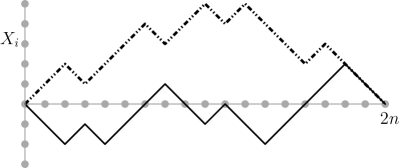
Figure 27: The zigzag solid line shows a random walk bridge of $2n=18$ steps that spends $2m=6$ steps on the positive side. The dashed line shows an excursion of $2n$ steps that is conditioned to stay positive, for the entire duration.

Appendix Q Uniform distribution of $t_{\rm pos}$ for a Brownian Bridge

In Sec. VIII.1 we used a result that for a Brownian bridge, time spent on positive half has a uniform distribution. Here, we give a derivation of this result.

Our derivation is for a random walk of total $2n$ steps on an infinite chain. The walker is conditioned to take equal number of positive and negative steps such that at the final step the walker returns to the starting point, which we choose to be the origin. Continuous limit of the process is a Brownian bridge, and the distribution of positive time for the Random walk gives the distribution for Brownian bridge in the continuous limit.

For our derivation, we define a generating function

$$G(\kappa,\rho)=1+\sum_{n=1}^{\infty}\sum_{m=0}^{n}\kappa^{n}\rho^{m}\frac{1}{2^{2n}}N(2n,2m),$$ (508)

where $(\kappa,\rho)$ are parameters and $N(2n,2m)$ gives the total number of Random walk bridges of length $2n$ with $2m$ number of steps spent on the positive side of the chain (see illustration in Fig. 27).

We define a second generating function

$$g(\kappa)=\sum_{n=1}^{\infty}\frac{\kappa^{n}}{2^{2n}}N^{+}(2n),$$ (509)

where $N^{+}(2n)$ gives the number of random bridges that stay on the positive side of the chain for the entire duration $2n$ (Random walk excursion. See illustration in Fig. 27).

Using method of images it is straightforward to show that

$$N^{+}(2n)=\binom{2n-2}{n-1}-\binom{2n-2}{n}=\frac{(2n-2)!}{n!(n-1)!},$$ (510)

leading to

$$g(\kappa)=\frac{1}{2}\left(1-\sqrt{1-\kappa}\right).$$ (511)

Figure 28: A graphical representation of the infinite summation in Eq. (515). Down-sided excursions represent $g(\kappa)$ and up-sided excursions represent $g(\kappa\,\rho)$. Relative order of excursions give the degeneracy in Eq. (515).

To calculate $G(\kappa,\rho)$ we use a relation

$$G(\kappa,\rho)= 1+\left[g(\kappa)+g(\kappa\rho)\right]+$$ (512)

$$\left[g(\kappa)^{2}+2g(\kappa)g(\kappa\rho)+g(\kappa\rho)^{2}\right]+$$ (513)

$$\left[g(\kappa)^{3}+3g(\kappa)^{2}g(\kappa\rho)+3g(\kappa)g(\kappa\rho)^{2}+g(\kappa\rho)^{3}\right]$$ (514)

$$+\cdots,$$ (515)

which can be seen by the graphical illustration in Fig. 28. Completing the summation we get

$$G(\kappa,\rho)=\frac{1}{1-g(\kappa)-g(\kappa\rho)}.$$ (516)

Using the formula for $g(\kappa)$ in Eq. (509) we write

$$G(\kappa,\rho)=1+\sum_{n=1}^{\infty}\sum_{m=0}^{n}\kappa^{n}\rho^{m}\frac{(2n)!}{2^{2n}(n+1)(n!)^{2}}.$$ (517)

Comparing with Eq. (508) it is evident that $N(2n,2m)$ is independent of $m$. Equivalently, there are equal number of paths for all values of $m$ in a random walk bridge of length $2n$. In the continuous limit, this means that for a Brownian bridge, all values of fractional positive time are equally probable.

References

- [1] L. Decreusefond and A.S. Üstünel, Fractional Brownian motion: Theory and applications, in ESAIM: PROC, pages 75–86, EDP Sciences, 1998.
- [2] H. Qian, Fractional Brownian motion and fractional gaussian noise, in Processes with Long-Range Correlations, pages 22–33, Springer, 2003.
- [3] I. Nourdin, Selected aspects of fractional Brownian motion, Bocconi & Springer Series, 2012.
- [4] G. Shevchenko, Fractional Brownian motion in a nutshell, Int. J. Mod. Phys. 36 (2015) 1560002.
- [5] A.N. Kolmogorov, Wienersche spiralen und einige andere interessante Kurven im Hilbertschen Raum, CR(Dokl.) Acad. Sci. URSS 26 (1940) 115–118.
- [6] B.B. Mandelbrot and J.W. Van Ness, Fractional Brownian motions, fractional noises and applications, SIAM Review 10 (1968) 422–437.
- [7] R. Metzler and J. Klafter, The random walk’s guide to anomalous diffusion: a fractional dynamics approach, Phys. Rep. 339 (2000) 1–77.
- [8] S. Cohen and J. Istas, Fractional Fields and Applications, Springer, 2013.
- [9] V. Kukla, J. Kornatowski, D. Demuth, I. Girnus, H. Pfeifer, L.V.C. Rees, S. Schunk, K.K. Unger and J. Karger, NMR studies of single-file diffusion in unidimensional channel zeolites, Science (1996) 702 –704.
- [10] Q.-H. Wei, C. Bechinger and P. Leiderer, Single-file diffusion of colloids in one-dimensional channels, Science 287 (2000) 625–627.
- [11] L Lizana, T. Ambjörnsson, A. Taloni, E. Barkai and M.A. Lomholt, Foundation of fractional Langevin equation: Harmonization of a many-body problem, Phys. Rev. E 81 (2010) 051118.
- [12] P.L. Krapivsky, K. Mallick and T. Sadhu, Dynamical properties of single-file diffusion, J. Stat. Mech. (2015) P09007, arXiv:1505.01287.
- [13] T. Sadhu and B. Derrida, Large deviation function of a tracer position in single file diffusion, J. Stat. Mech. 2015 (2015) P09008.
- [14] T. Sadhu and B. Derrida, Correlations of the density and of the current in non-equilibrium diffusive systems, J. Stat. Mech. 2016 (2016) 113202.
- [15] A. Zoia, A. Rosso and S.N. Majumdar, Asymptotic behavior of self-affine processes in semi-infinite domains, Phys. Rev. Lett. 102 (2009) 120602.
- [16] J.L.A. Dubbeldam, V.G. Rostiashvili, A. Milchev and T.A. Vilgis, Fractional Brownian motion approach to polymer translocation: The governing equation of motion, Phys. Rev. E 83 (2011) 011802.
- [17] V. Palyulin, T. Ala-Nissila and R. Metzler, Polymer translocation: the first two decades and the recent diversification, Soft Matter 10 (2014) 9016–9037.
- [18] J.-P. Bouchaud and A. Georges, Anomalous diffusion in disordered media: statistical mechanisms, models and physical applications, Phys. Rep. 195 (1990) 127–293.
- [19] E.E. Peters, Chaos and order in the capital markets, Wiley finance editions, Wiley, New York, 2 edition, 1996.
- [20] N.J. Cutland, P.E. Kopp and W. Willinger, Stock price returns and the Joseph effect: A fractional version of the Black-Scholes model, in E. Bolthausen, M. Dozzi and F. Russo, editors, Seminar on Stochastic Analysis, Random Fields and Applications, Volume 36 of Progress in Probability, pages 327–351, Birkhäuser Basel, 1995.
- [21] F. Biagini, Y Hu, B. Oksendal and T. Zhang, Stochastic Calculus for Fractional Brownian Motion and Applications, Springer Verlag, London, 2008.
- [22] T. Sottinen, Fractional Brownian motion, random walks and binary market models, Finance and Stochastics 5 (2001) 343–355.
- [23] H.E. Hurst, Long-term storage capacity of reservoirs, Transactions of the American Society of Civil Engineers 116 (1951) 770–799.
- [24] B.B. Mandelbrot and J.R. Wallis, Noah, Joseph, and operational hydrology, Water Resources Research 4 (1968) 909–918.
- [25] S. Gupta, A. Rosso and C. Texier, Dynamics of a tagged monomer: Effects of elastic pinning and harmonic absorption, Phys. Rev. Lett. 111 (2013) 210601.
- [26] E. Monte-Moreno and M. Hernández-Pajares, Occurrence of solar flares viewed with gps: Statistics and fractal nature, J. Geophys. Res. 119 (2014) 9216–9227.
- [27] I. Simonsen, Measuring anti-correlations in the nordic electricity spot market by wavelets, Physica A 322 (2003) 597–606.
- [28] I. Norros, On the use of fractional Brownian motion in the theory of connectionless networks, IEEE J. Sel. A. Commun. 13 (2006) 953–962.
- [29] K. Burnecki, E. Kepten, J. Janczura, I. Bronshtein, Y. Garini and A. Weron, Universal algorithm for identification of fractional brownian motion. a case of telomere subdiffusion, Biophysical Journal 103 (2012) 1839–1847.
- [30] J.H. Jeon, V. Tejedor, S. Burov, E. Barkai, C. Selhuber-Unkel, K. Berg-Sørensen, L. Oddershede and R. Metzler, In vivo anomalous diffusion and weak ergodicity breaking of lipid granules, Phys. Rev. Lett. 106 (2011) 048103.
- [31] D. Ernst, M. Hellmann, K. Jürgen and M. Weiss, Fractional Brownian motion in crowded fluids, Soft Matter 8 (2012) 4886–4889.
- [32] G. M. Molchan, Maximum of a fractional Brownian motion: Probabilities of small values, Comm. Math. Phys. 205 (1999) 97–111.
- [33] J. Krug, H. Kallabis, S.N. Majumdar, S. J. Cornell, A. J. Bray and C. Sire, Persistence exponents for fluctuating interfaces, Phys. Rev. E 56 (1997) 2702–2712.
- [34] T. Guérin, N. Levernier, O. Bénichou and R. Voituriez, Mean first-passage times of non-Markovian random walkers in confinement, Nature 534 (2016) 356–359.
- [35] S.N. Majumdar, Brownian functionals in physics and computer science, in The Legacy of Albert Einstein., Volume 89, pages 93–129, World scientific, 2005, arXiv:cond-mat/0510064.
- [36] T. Hida, Functionals of Brownian motion, in J. Kožešnik, editor, Transactions of the Seventh Prague Conference on Information Theory, Statistical Decision Functions, Random Processes and of the 1974 European Meeting of Statisticians: held at Prague, from August 18 to 23, 1974, pages 239–243, Springer Netherlands, Dordrecht, 1977.
- [37] D. Ruelle, Smooth dynamics and new theoretical ideas in nonequilibrium statistical mechanics, J. Stat. Phys. 95 (1999) 393–468.
- [38] D. Ruelle, Conversations on Nonequilibrium Physics With an Extraterrestrial, Phys. Today 57 (2004) 48–53.
- [39] J.L. Lebowitz and H. Spohn, A Gallavotti–Cohen-type symmetry in the large deviation functional for stochastic dynamics, J. Stat. Phys. 95 (1999) 333–365.
- [40] P. Lévy, Sur certains processus stochastiques homogènes, Compositio Mathematica 7 (1940) 283–339.
- [41] W. Feller, Introduction to Probability Theory and Its Applications, John Wiley & Sons, 1950.
- [42] P. Mörters and Y. Peres, Brownian Motion, Cambridge University Press, 2010.
- [43] J.Y. Yen and M. Yor, Paul Lévy’s Arcsine Laws, pages 43–54, Springer International Publishing, Cham, 2013.
- [44] S.N. Majumdar, J. Randon-Furling, M.J. Kearney and M. Yor, On the time to reach maximum for a variety of constrained Brownian motions, J. Phys. A 41 (2008) 365005.
- [45] S. N. Majumdar and J. P. Bouchaud, Optimal time to sell a stock in the black–scholes model: comment on ‘Thou shalt buy and hold’, by A. Shiryaev, Z. Xu and X. Y. Zhou, Quantitative Finance 8 (2008) 753–760.
- [46] J. Randon-Furling and S.N. Majumdar, Distribution of the time at which the deviation of a Brownian motion is maximum before its first-passage time, J. Stat. Mech. 2007 (2007) P10008.
- [47] S.N. Majumdar, Universal first-passage properties of discrete-time random walks and Lévy flights on a line: Statistics of the global maximum and records, Physica A 389 (2010) 4299–4316.
- [48] G. Schehr and P. Le Doussal, Extreme value statistics from the real space renormalization group: Brownian motion, Bessel processes and continuous time random walks, J. Stat. Mech. 2010 (2010) P01009, arXiv:0910.4913.
- [49] K. J. Hochberg and E. Orsingher, The arcsine law and its analogs for processes governed by signed and complex measures, Stoch. Proc. App. 52 (1994) 273–292.
- [50] J. Pitman and M. Yor, Arcsine laws and interval partitions derived from a stable subordinator, Proc. London Math. Soc (1992) 65–326.
- [51] P. Carmona, F. Petit and M. Yor, Some extensions of the arcsine law as partial consequences of the scaling property of Brownian motion, Prob. Theo. Rel. Fields 100 (1994) 1–29.
- [52] J. Lamperti, An occupation time theorem for a class of stochastic processes, Trans. Amer. Math. Soc. 88 (1958) 380–387.
- [53] M. Barlow, J. Pitman and M. Yor, Une extension multidimensionnelle de la loi de tare sinus, in Siminaire de Probabilites XXIII, pages 294–314, Springer, Berlin, 1989.
- [54] N. H. Bingham and R. A. Doney, On higher-dimensional analogues of the arcsine law, J. App. Prob. 25 (1988) 120–131.
- [55] P. A. Ernst and L. Shepp, On occupation times of the first and third quadrants for planar Brownian motion, J. Appl. Prob. 54 (2017) 337–342.
- [56] D. Charles and W. Rosemarie, The arcsine law and the treasury bill futures market, Financial Analysts Journal 36 (1980) 71–74.
- [57] J. Baz and G. Chacko, Financial Derivatives: Pricing, Applications, and Mathematics, Cambridge University Press, 2004.
- [58] A. Clauset, M. Kogan and S. Redner, Safe leads and lead changes in competitive team sports, Phys. Rev. E 91 (2015) 062815–062826.
- [59] K.J. Wiese, S.N. Majumdar and A. Rosso, Perturbation theory for fractional Brownian motion in presence of absorbing boundaries, Phys. Rev. E 83 (2011) 061141, arXiv:1011.4807.
- [60] M. Delorme and K.J. Wiese, Maximum of a fractional Brownian motion: Analytic results from perturbation theory, Phys. Rev. Lett. 115 (2015) 210601, arXiv:1507.06238.
- [61] M. Delorme and K.J. Wiese, Extreme-value statistics of fractional Brownian motion bridges, Phys. Rev. E 94 (2016) 052105, arXiv:1605.04132.
- [62] M. Delorme and K.J. Wiese, Perturbative expansion for the maximum of fractional Brownian motion, Phys. Rev. E 94 (2016) 012134, arXiv:1603.00651.
- [63] M. Delorme, A. Rosso and K.J. Wiese, Pickands’ constant at first order in an expansion around Brownian motion, J. Phys. A 50 (2017) 16LT04, arXiv:1609.07909.
- [64] M. Delorme, Stochastic processes and disordered systems, around Brownian motion, PhD thesis, PSL Research University, 2016.
- [65] K.J. Wiese, First passage in an interval for fractional Brownian motion, Phys. Rev. E 99 (2018) 032106, arXiv:1807.08807.
- [66] M. Arutkin, B. Walter and K.J. Wiese, Extreme events for fractional Brownian motion with drift: Theory and numerical validation, Phys. Rev. E 102 (2020) 022102, arXiv:1908.10801.
- [67] T. Sadhu, M. Delorme and K.J. Wiese, Generalized arcsine laws for fractional Brownian motion, Phys. Rev. Lett. 120 (2018) 040603, arXiv:1706.01675.
- [68] M. Kac, On distributions of certain Wiener functionals, Trans. Amer. Math. Soc. 65 (1949) 1–13.
- [69] J. Zinn-Justin, Quantum Field Theory and Critical Phenomena, Oxford University Press, Oxford, 1989.
- [70] R.B. Davies and D.S. Harte, Tests for hurst effect, Biometrika 74 (1987) 95–101.
- [71] A.B. Dieker, Simulation of fractional Brownian motion, PhD thesis, University of Twente, 2004.
- [72] B. Walter and K.J. Wiese, Monte Carlo sampler of first passage times for fractional Brownian motion using adaptive bisections: Source code, hal-02270046 (2019).
- [73] B. Walter and K.J. Wiese, Sampling first-passage times of fractional Brownian motion using adaptive bisections, Phys. Rev. E 101 (2020) 043312, arXiv:1908.11634.
- [74] A. Dhar and S.N. Majumdar, Residence time distribution for a class of gaussian markov processes, Phys. Rev. E 59 (1999) 6413–6418.
- [75] D. B. Owen, Orthant probabilities, in Wiley StatsRef: Statistics Reference Online, American Cancer Society, 2014.
- [76] T. Sadhu and K.J. Wiese, Supplemental mathematica notebook which describes certain steps to evaluate expresion for .
- [77] S.N. Majumdar and A. Comtet, Airy Distribution Function: From the Area Under a Brownian Excursion to the Maximal Height of Fluctuating Interfaces, J. Stat. Phys. 119 (2005) 777–826.
- [78] J.F. Coeurjolly, Simulation and identification of the fractional Brownian motion: a bibliographical and comparative study, Journal of Statistical Software 05 (2000) i07.
- [79] A.T.A. Wood and G. Chan, Simulation of stationary gaussian processes in , Journal of Computational and Graphical Statistics 3 (1994) 409–432.