Kinetic Monte Carlo Algorithms for Active Matter systems

Abstract

We study kinetic Monte Carlo (KMC) descriptions of active particles. We show that, when they rely on purely persistent, active steps, their continuous-time limit is ill-defined, leading to the vanishing of trademark behaviors of active matter such as the motility-induced phase separation, ratchet effects, as well as to a diverging mechanical pressure. We then show how, under an appropriate scaling, mixing passive steps with active ones leads to a well-defined continuous-time limit that however differs from standard active dynamics. Finally, we propose new KMC algorithms whose continuous-time limits lead to the dynamics of active Ornstein-Uhlenbeck, active Brownian, and run-and-tumble particles.

Monte Carlo (MC) methods are widely popular across disciplines [1, 2]. At equilibrium, detailed balance is enforced and unphysical dynamics can be used while preserving the steady-state Boltzmann distribution. Unphysical tricks can then be exploited to accelerate equilibration without altering steady-state averages of one-time observables, a property which has led to many breakthroughs in equilibrium statistical physics [3, 4, 5]. MC algorithms have also been used to study diverse nonequilibrium phenomena like coarsening [6, 7, 8], slow relaxation in disordered systems [9, 10, 11], granular media [12, 13, 14, 15], self-assembly [16], gel electrophoresis of DNA [17], or surface properties [18]. However, the relevance of discrete-time dynamics for nonequilibrium systems is questionable [19, 20, 21] since no detailed-balance symmetry enforces a steady-state distribution that is independent from the MC dynamics. This question is particularly relevant in the field of active matter, where MC simulations have been used extensively to simulate the collective dynamics of active particles [22, 23, 24, 25, 26, 27, 28, 29, 30, 31, 32, 33, 34, 35].

Active matter constitutes a class of biological and synthetic systems that are driven out of equilibrium at the microscopic scale [36, 37, 38]. In their simplest form, they comprise assemblies of particles that dissipate energy to exert self-propelling forces, hence breaking the fluctuation-dissipation relation that would otherwise drive the dynamics of passive colloids towards Boltzmann equilibrium. Active systems have attracted a lot of attention due to their rich phenomenologies, ranging from collective motion [39, 40], to phase separation in the absence of cohesive forces  [41], to spatiotemporal chaos at zero Reynolds number [42, 43, 44].

The study of active matter systems is, however, challenging because of two important limitations. Theoretically, first, there is no generic expression for the steady-state distribution of active systems and no counterpart to the Boltzmann weight to guide our intuition. Numerically, then, studying the large-scale properties of active systems requires sampling sizes much larger than the particle persistence length. Defined as the typical distance a particle travels before it forgets its initial orientation, the persistence length often has to be much larger than the particle size for active matter to display its most exciting features. This makes the system sizes to be simulated much larger than for passive systems [45, 46, 47, 48, 34, 35].

To address this problem, a natural strategy would be, following the success of MC in equilibrium, to replace the continuous-time setting in which active dynamics are naturally defined by MC dynamics in which time has been coarse grained. Several attempts along these lines have been introduced recently, in particular to study motility-induced phase separation (MIPS) [25, 30], the two-dimensional melting [30, 33, 49], and high-density binary mixtures [26]. All these approaches however suffer from a major drawback: unlike for equilibrium systems, nothing guarantees that these MC dynamics, even in the proper limit, correspond to bona fide continuous-time active dynamics.

In this Letter, we bridge this gap by providing a class of active kinetic MC dynamics (AKMC) whose continuous-time limit—which we construct explicitly—is shown to encompass the celebrated run-and-tumble (RT) [50, 51], active Brownian (AB) [52, 53] and active Ornstein-Uhlenbeck (AOU) [54, 55] dynamics. To do so, we start by analyzing the continuous-time limit of AKMC algorithms that have attracted a lot of attention recently [25, 26, 27, 30, 49, 33]. We first show numerically and analytically that algorithms relying exclusively on correlated, ‘active’ steps lead to an ill-defined continuous-time limit. We then show how the introduction of a finite fraction of uncorrelated ‘passive’ steps, together with a rescaling of the propulsion speed, leads to a well-defined continuous active dynamics. Importantly, the latter describes a new class of active particles that differ from AB, RT, and AOU particles, notwithstanding [25, 26, 27]. We close the Letter by discussing how our AKMC can be modified to lead to RT, AB, and AOU particles hence providing a generic toolbox to simulate active dynamics using AKMCs.

Active kinetic Monte Carlo dynamics— We consider a system of $N$ active particles endowed with the following dynamics, adapted from [25, 30]. At every time step $t_{n}=ndt$, $N$ particles are successively chosen at random and their positions ${\bf r}_{i}$ and self-propulsion velocities ${\bf v}_{i}$ are updated, in this order. A particle at ${\bf r}$ moves to a new position ${\bf r}+{\bf v}dt$, with probability

$$f({\bf r},{\bf v}dt)=\min\left[1,\exp\left(-\beta\Delta U({\bf r}\to{\bf r}+{\bf v}dt)\right)\right]\,,$$ (1)

where $\beta$ is a control parameter and $\Delta U=U({\bf r}+{\bf v}dt)-U({\bf r})$ is the total energy change. Equation (1) is nothing but a standard equilibrium Metropolis filter, in the context of which $\beta$ would be the inverse temperature, and the breakdown of detailed balance comes from the dynamics of ${\bf v}$. A new velocity ${\bf v}(t_{n+1})$ is sampled from a Gaussian distribution centered at ${\bf v}(t_{n})$, of standard deviation $\delta v=\sqrt{2D_{v}dt}$, which is then folded back using reflecting boundary conditions at $|{\bf v}|=v_{0}$. (See Fig. S1 in [56] for an illustration of this procedure.) Successive particle displacements are thus correlated, hence leading to a persistent motion characterized, in two space dimensions, by a persistence time $\tau=\frac{v_{0}^{2}}{c^{2}D_{v}}$ where $c$ is a constant that can be computed exactly (see SM [56]).

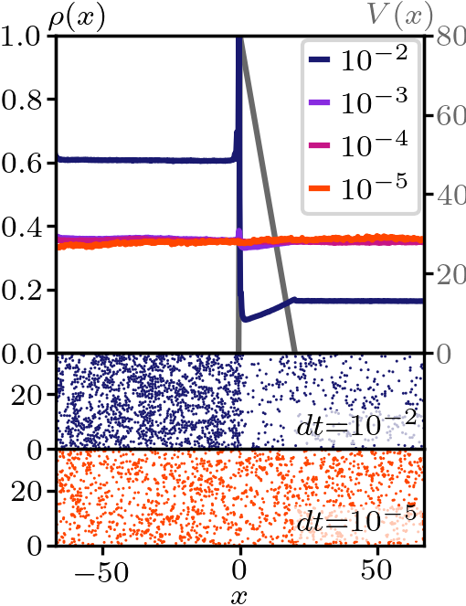
(a)

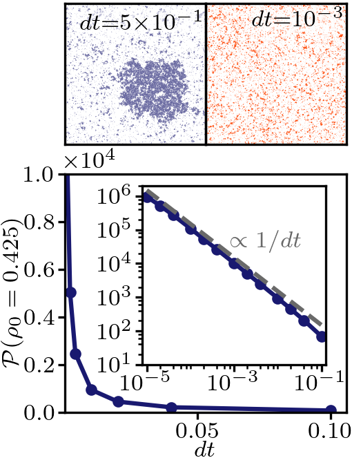
(b)

Figure 1: Simulations of $N$ interacting active particles in $2D$ using the AKMC with $\beta=1$. (a) As $dt$ is decreased from $10^{-2}$ to $10^{-5}$, the pumping effect induced by an asymmetric potential $V(x)$ (solid gray line, upper panel, explicit expression given in SM [56]) disappears, as can be seen by comparing our simulations for $dt=10^{-2}$ (snapshot in center panel and density profile shown as blue line in upper panel) and for $dt=10^{-5}$ (snapshot in lower panel and density profile shown as red line in upper panel). Parameters: $\tau=1$, $v_{0}=4$, average number density $\rho_{0}\simeq 0.36$; periodic (resp. closed) boundary conditions are used along $y$ (resp. $x$). (b) MIPS is observed for $dt=0.5$ (blue, left panel) but not for $dt=0.001$ (red, right panel), using periodic boundary conditions. Parameters: $\tau=200$, $v_{0}=1$, $N=43\,904$, $L=468$. (c) The mechanical pressure exerted on a confining potential $U_{\rm w}(x,y)=\frac{\Omega}{\nu}(x\pm x_{\rm w})^{\nu}\quad\text{for}\quad|x|>x_{\rm w}\;$ is measured using Eq. (2) at bulk number density $\rho_{0}=0.425$ using periodic boundaries along $y$. It diverges as $1/dt$ when $dt\to 0$. Parameters: $\tau=10$, $v_{0}=1$, $L_{y}=32$, $x_{\rm w}=64$, $\Omega=10$, $\nu=8$.

Figure 1 shows AKMC simulations of $N$ particles interacting via a Weeks-Chandler-Andersen potential $U(r)=4\left[(\sigma/r)^{12}-(\sigma/r)^{6}\right]+1$ for $r<2^{1/6}\sigma$ and $U(r)=0$ otherwise, with $\sigma=2^{-1/6}$. Simulations are shown for different time steps $dt$, keeping the self-propulsion speed $v_{0}$ and persistence time $\tau$ constant. Using large time steps, the simulations reproduce standard features of active systems: motility-induced phase separation [41] is observed and asymmetric obstacles are able to pump particles, hence generating long-ranged perturbations to the density field [57, 58, 59]. However, both features disappear for smaller time steps. Even more surprising, the mechanical pressure exerted by the particles on a confining potential $U_{\rm w}$, measured as [60]

$$\mathcal{P}=\int_{x_{\rm bulk}}^{\infty}\rho(x)\partial_{x}U_{\rm w}(x)\,,$$ (2)

is shown to diverge when $dt\to 0$. The AKMC algorithm introduced in this section is thus not suitable to describe active dynamics.

Vanishing mobility in the continuous-time limit— This pathological behavior can be understood analytically by showing that the particle mobility vanishes as $dt\to 0$, making the particles less and less sensitive to forces other than the self-propulsion ones. Let us consider the simpler problem of an isolated particle in the presence of an external potential $U(x)$ in one space dimension. The generalization to higher dimensions and interacting particles is straightforward. Reformulating the AKMC in one dimension leads to a persistence time $\tau=4v_{0}^{2}/(\pi^{2}D_{v})$ [56]. We denote $P_{n}(x,v)$ the probability density to find the particle at position $x$ with velocity $v$ at time $t_{n}$. Its evolution is given by

$$P_{n+1}(x,v)=\int dx^{\prime}dv^{\prime}g(v|v^{\prime})W(x|x^{\prime},dt\,v^{\prime})P_{n}(x^{\prime},v^{\prime})$$ (3)

where $g(v|v^{\prime})$ is the probability density to transition from self-propulsion velocity $v^{\prime}$ to $v$ and where

$$W(x|x^{\prime},\Delta x) \equiv f(x^{\prime},\Delta x)\delta(x^{\prime}+\Delta x-x)$$ (4)

$$+[1-f(x^{\prime},\Delta x)]\delta(x^{\prime}-x)$$

is the probability density to transition from $x^{\prime}$ to $x$. The two terms on the rhs of Eq. (4) correspond to hopping from $x^{\prime}\neq x$ into $x$ and to staying in $x^{\prime}$, respectively.

The continuous-time limit of the evolution equation is obtained by truncating the Kramers-Moyal expansion of $\Delta P\equiv P_{n+1}(x,v)-P_{n}(x,v)$ to first order in $dt$ [61, 62]. This has been done with success for equilibrium MC dynamics—see e.g. [63, 19, 20], or [64] for a nice application to neural networks. As we show in the following, the generalization of this approach to the active case leads to the Fokker-Planck equation [65]:

$$\partial_{t}P(x,v;t)=-\frac{\partial}{\partial x}[vP(x,v;t)]+D_{v}\frac{\partial^{2}}{\partial v^{2}}P(x,v;t)\,,$$ (5)

which is complemented by a zero-current condition

$$\partial_{v}P(x,v;{t})|_{v=\pm v_{0}}=0\;.$$ (6)

The main lesson of this calculation is that the confining potential drops out from Eq. (5). To understand better how this happens, it is insightful to write $\Delta P$ as

$$\Delta P = \int dv^{\prime}g(v|v^{\prime})[f(x-v^{\prime}dt,v^{\prime}dt)P_{n}(x-v^{\prime}dt,v^{\prime})$$ (7)

$$-f(x,v^{\prime}dt)P_{n}(x,v^{\prime})]$$

$$+\int dv^{\prime}g(v|v^{\prime})P_{n}(x,v^{\prime})-P_{n}(x,v)\;.$$

Consider first the last line of Eq. (7). Taylor expanding $P_{n}(x,v^{\prime})$ close to $v^{\prime}=v$ leads to

$$\int dv^{\prime}g(v|v^{\prime})P_{n}(x,v^{\prime})-P_{n}(x,v)=\sum_{k>0}\frac{a_{k}}{k!}\partial_{v}^{k}P_{n}(x,v)\,,$$

where $a_{k}$ is related to the $k^{\rm th}$ moment of the change in velocity through $a_{k}=(-1)^{k}\int dv^{\prime}g(v|v^{\prime})(v-v^{\prime})^{k}$. The coefficient $a_{1}$ vanishes by symmetry in the $dt\to 0$ limit and $a_{2}=\delta v^{2}$ provides the dominant order to $\Delta P$. This confirms the scaling $\delta v=\sqrt{2dtD_{v}}$ chosen above and leads to the Laplacian on $v$ in Eq. (5). The zero-flux condition on $v$ is simply inherited from that of the discrete-time process [61]. Consider now the first two lines of Eq. (7). To leading order in $dt$, they are equivalent to $-dt\int dv^{\prime}g(v|v^{\prime})v^{\prime}\partial_{x}[f(x,v^{\prime}dt)P_{n}(x,v^{\prime})]$. This is already of order $dt$ so that only the ${\cal O}(1)$ contribution of the integral survives. To estimate the latter, we first note that $\Delta U\simeq vdtU^{\prime}(x)$ so that the Metropolis filter can be approximated as $f(x,vdt)\simeq 1-\beta vdtU^{\prime}(x)\frac{1+{\rm sgn}(\Delta U)}{2}$. To leading order, $f=1$ and the AKMC is insensitive to the filter in the continuous-time limit. The computation can then be concluded by using that $v^{\prime}=(v^{\prime}-v)+v$ and Taylor expanding $P(x,v^{\prime})$ at $v^{\prime}=v$, yielding a leading order contribution $-dtv\partial_{x}P(x,v)$. Mathematically, $U$ thus only enters Eq. (5) at the next order in $dt$: the mobility of this AKMC vanishes linearly in $dt$. Physically, $U$ is ignored by the particles since a succession of infinitely small persistent steps lead to their systematic acceptance.

The derivation above explains both the uniform distribution measured in Fig. 1a and the suppression of MIPS in Fig. 1b. Furthermore, as $dt\to 0$, particles penetrate more and more into confining walls, so that the mechanical pressure exerted on the walls, measured as Eq. (2), diverges.

A blended AKMC— Since KMC algorithms admit a well-defined continuous-time limit in equilibrium [63, 19, 20, 21, 64], it is natural to try and interpolate between passive and active KMC dynamics [25]. To do so, we introduce a blended AKMC as follows. At every time step, an attempt to move from $x$ to $x+vdt/\alpha$ is done with probability $\alpha$ whereas a move from $x$ to $x+\xi$ is attempted with probability $1-\alpha$, where $\xi$ is sampled uniformly and independently at each time step in $[-\sqrt{6Ddt/(1-\alpha)},\sqrt{6Ddt/(1-\alpha)}]$. In both cases, the move is accepted or rejected using the Metropolis filter defined in (1). Note that the rescaling of the propulsion speed and of the passive diffusivities with $\alpha$ will be proved below to be crucial to the existence of an $\alpha$-independent well-defined continuous-time limit. Figure 2 shows simulation results for $\alpha=0.4$ and $\alpha=0.6$. Motility-induced phase separation and a long-range modulation of the density field by an asymmetric obstacle are again observed for large $dt$. This time, however, these phenomena are stable as $dt\to 0$. The mechanical pressure exerted on confining walls also admits a well-defined limit.

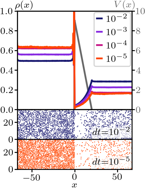
(a)

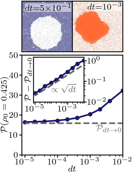
(b)

Figure 2: Simulations of $N$ interacting active particles using the blended AKMC with $\beta=1$ and $\alpha\in(0,1)$. (a) As $dt$ is decreased from $10^{-2}$ to $10^{-5}$, the pumping effect induced by an asymmetric potential $V(x)$ (gray line, upper panel, explicit expression given in SM [56]) is now converging to a stable nonequilibrium steady state. Parameters: $\alpha=0.4$, $\tau=1$, $v_{0}=4$, $D=1$, $\rho_{0}\simeq 0.36$. Periodic (resp. closed) boundary conditions are implemented along $y$ (resp. $x$). (b) MIPS is now observed both for $dt=0.5$ (blue, left panel) and $dt=0.001$ (red, right panel), using periodic boundary conditions. Parameters: $\alpha=0.6$, $\tau=200$, $v_{0}=1$, $D=0.05$, $N=43\,904$, $L=270$. (c) The mechanical pressure exerted on the confining potential $U_{\rm w}$ is measured using Eq. (2) and has now a well-defined limit as $dt\to 0$. Parameters: $\alpha=0.6$, $\tau=10$, $v_{0}=1$, $D=0.05$. The same geometry, wall potential, and densities are used as in Fig. 1(c).

The continuous-time limit of the blended AKMC can be constructed analytically from the following extension of our calculation. The master equation now writes

$$P_{n+1}(x,v)=\alpha\int dx^{\prime}dv^{\prime}g(v|v^{\prime})W\Big{(}x\Big{|}x^{\prime},{\frac{v^{\prime}dt}{\alpha}}\Big{)}P_{n}(x^{\prime},v^{\prime})$$

$$+(1-\alpha)\int dx^{\prime}dv^{\prime}d\xi g(v|v^{\prime})W(x|x^{\prime},\xi)P_{n}(x^{\prime},v^{\prime})G(\xi)\,,$$ (8)

where $G(\xi)$ is the uniform measure over $[-\sqrt{6Ddt/(1-\alpha)},\sqrt{6Ddt/(1-\alpha)}]$. By linearity, the continuous-time limit of this blended AKMC is now readily obtained. The first line of Eq. (8) again leads to the drift and diffusion terms derived in Eq. (5), albeit the latter multiplied by $\alpha$. The second line still leads to the diffusion of the self-propulsion velocity multiplied by $(1-\alpha)$, but also to the standard terms entering the Fokker-Planck equation of a passive particle. All in all, this leads to the Fokker-Planck equation

$$\partial_{t}P_{t}(x,v) =-\partial_{x}\left[\left\{v+\mu F(x)\right\}P_{t}(x,v)\right]+$$ (9)

$$D\partial_{x}^{2}P_{t}(x,v)+D_{v}\partial_{v}^{2}P_{t}(x,v)$$

where Eq. (9) is again supplemented by the zero-current condition in Eq. (6). This time, the confining force $F(x)=-\partial_{x}U(x)$ survives in the $dt\to 0$ limit thanks to a finite mobility $\mu=\beta D$. Interestingly, comparing Eqs. (5) and (9) shows that the role played by the passive steps to restore the continuous-time limit is not so much the introduction of translational diffusion as the restoration of a finite mobility.

We now compute the mechanical pressure predicted by Eq. (9) to check that the latter quantitatively describes the small $dt$ limit of the blended AKMC. Integrating over $v$ and using the zero-flux condition along $x$ imposed by the confining wall leads to $\rho(x)U_{\rm w}^{\prime}(x)=-\tfrac{D}{\mu}\rho^{\prime}(x)+{\tfrac{1}{\mu}}\bar{v}_{1}(x)$, where we define $\bar{v}_{k}(x)=\int dvP(x,v)v^{k}$ and $\rho(x)=\bar{v}_{0}(x)$. Further integrating from $x=0$ to $x=\infty$ leads to ${\mathcal{P}}=\frac{D}{\mu}\rho_{0}+{\tfrac{1}{\mu}}\int_{0}^{\infty}\bar{v}_{1}(x)dx$. To compute the last integral, we multiply Eq. (9) by $v^{k}$ and integrate over $v$ to get, in the steady state,

$$(k-1)\bar{v}_{k-2}=v_{0}^{k-1}[P(x,v_{0})+(-1)^{k}P(x,-v_{0})]+\partial_{x}\frac{J_{k}}{kD_{v}}\;,$$ (10)

where $J_{k}\equiv\bar{v}_{k+1}-\bar{v}_{k}\mu U_{\rm w}^{\prime}(x)-D\partial_{x}\bar{v}_{k}$. For $k=1$, Eq. (10) leads to $[P(x,v_{0})-P(x,-v_{0})]=-\partial_{x}J_{1}/D_{v}$. Injecting this into Eq. (10) for $k=3$ and integrating both sides of the equation from $x=0$ to $\infty$ leads to $6D_{v}\int_{0}^{\infty}\bar{v}_{1}dx=[3v_{0}^{2}\bar{v}_{2}(0)-\bar{v}_{4}(0)]$. Since the bulk of the system is homogeneous and isotropic, $P(x=0,v)=\rho_{0}/(2v_{0})$ and the mechanical pressure reads

$${\mathcal{P}}=\rho_{0}\left(k_{\rm B}T+\frac{2v_{0}^{4}}{15\mu D_{v}}\right)\;,$$ (11)

where we have introduced $k_{\rm B}T\equiv\beta^{-1}$. Figure 3a shows the perfect match between Eq. (11) and the mechanical pressure measured in numerical simulations for five different potential stiffnesses and several values of $\alpha\in(0,1)$. For $\alpha<1$, the pressure does not depend on the potential, which indicates that the blended AKMC satisfies an equation of state in the continuous-time limit. Note that the dependencies on $\alpha$ of the active steps, ${\bf r}\to{\bf r}+{\bf v}dt/\alpha$, and of the amplitude of the passive ones, $\xi\in[-\sqrt{6Ddt/(1-\alpha)},\sqrt{6Ddt/(1-\alpha)}]$, may look surprising at first glance—they were indeed absent in previous AKMCs [25, 30]. They are, however, crucial to lead to continuous-time limits independent of $\alpha$, as shown from Eq. (9) and illustrated in Fig. 3.

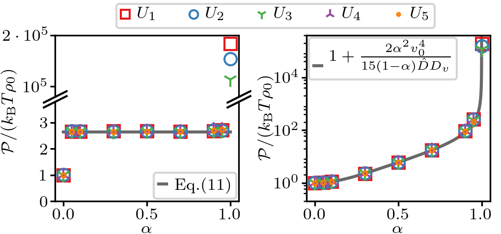
Figure 3: Mechanical pressure $\mathcal{P}$, defined in Eq. (2) and normalized by its equilibrium value $\mathcal{P}=\rho_{0}k_{\rm B}T$, measured as a function of the fraction of active steps $\alpha$ for noninteracting particles in 1d, with $\beta=1$, $v_{0}=1$, $\tau=5$, $dt=10^{-4}$. Symbols are measurements for several confining potentials $U_{1}$ to $U_{5}$, corresponding to the potential $U_{\rm w}$ defined in Fig. 1 with $(\nu,\Omega)$ given by $\{(8,10),\,(6,10),\,(4,10),\,(2,100),\,(2,10)\}$, respectively. The confining walls are located at $\pm x_{\text{w}}$. (a) Simulations carried out with the blended AKMC for $\alpha\in(0,1)$, $D=1$, and $x_{\text{w}}=15$. The limiting cases $\alpha=0$ and $\alpha=1$ correspond to purely passive and purely active KMCs, respectively. The solid gray line is the prediction of Eq. (11). (b) Simulations carried out without rescaling the active steps and the passive diffusivity, using instead $x(t_{n+1})\to x(t_{n})+vdt$ and $\xi\in[-\sqrt{6\hat{D}dt},\sqrt{6\hat{D}dt}]$, where $\hat{D}=1/6$ and $x_{\text{w}}=5$. The lack of rescaling leads to an unphysical dependency of the pressure on $\alpha$.

AB, RT, and AOU algorithms. We have shown that our blended AKMC leads to the Fokker-Planck equation (9) in the continuous-time limit. In two space dimensions, this active dynamics is equivalent to the Langevin equation

$$\dot{{\bf r}}={\bf v}-\mu\nabla U({{\bf r}})+\sqrt{2D}\bm{\eta};\quad\dot{\bf v}=\sqrt{2D_{v}}\bm{\zeta}$$ (12)

where $\bm{\eta}$ and $\bm{\zeta}$ are two uncorrelated unitary Gaussian white noises and ${\bf v}$ experiences reflecting boundary conditions at $|{\bf v}|=v_{0}$. Interestingly, the dynamics of ${\bf v}$ corresponds to none of the standard active particle models. As we now show, our blended AKMC can be adapted to yield discrete-time versions of AB, RT and AOU particles by solely modifying the dynamics of the self-propulsion speed. For RT and AB dynamics, the self-propulsion speed ${\bf v}(t_{n})$ lives on a circle of radius $v_{0}$ and is parametrized by an angle $\theta(t_{n})$. A discretized RT dynamics with tumbling rate $\gamma$ is obtained by choosing $\theta(t_{n+1})=\theta(t_{n})$ with probability $(1-\gamma dt)$ and by sampling $\theta(t_{n+1})$ uniformly in $[0,2\pi)$ with probability $\gamma dt$. To implement an AB dynamics with rotational diffusivity $D_{r}$, $\theta(t_{n+1})$ is sampled from a wrapped Gaussian distribution of standard deviation $\delta\theta=\sqrt{2D_{r}dt}$, centered at $\theta(t_{n})$. Finally, the AOU dynamics can be implemented as follows. A change of velocity ${\bf\delta v}(t_{n})$ is sampled uniformly in $[-\sqrt{6D_{\rm a}dt/(\tau^{2})},\sqrt{6D_{\rm a}dt/(\tau^{2})}]^{2}$. It is accepted with probability

$$p=\text{min}\Big{[}1,\exp\Big{(}-\frac{\tau^{2}}{D_{\rm a}}\Delta U_{v}[{\bf v}(t_{n})\to{\bf v}(t_{n})+{\bf\delta v}(t_{n})]\Big{)}\Big{]}$$ (13)

where $U_{v}({\bf v})=\frac{1}{2\tau}{\bf v}^{2}$. Carrying out the continuous-time limit of the dynamics indeed leads to the Fokker-Planck equation equivalent to $\dot{\bf r}={\bf v}+\mu{\bf F}+\sqrt{2D}\bm{\eta}$ and $\tau\dot{\bf v}=-{\bf v}+\sqrt{2D_{\rm a}}\bm{\zeta}$ where $\bm{\eta}$ and $\bm{\zeta}$ are two uncorrelated unitary Gaussian white noises.

Altogether we have shown how mixing passive steps with active ones endow AKMCs with bona fide continuous-time limits which encompass the workhorse models of active matter. By clarifying the connection between discrete and continuous-time dynamics, we believe our work will trigger a wider use of AKMCs in active matter. They should prove especially useful in the high density limit where Langevin equations are particularly difficult to use. This regime has indeed attracted a lot of attention recently [66, 67, 68, 69], in particular due to its relevance to the modeling of confluent tissues [70, 71, 72], but also because of the emergence of nontrivial spatial velocity correlations [73, 74, 75]. Finally, it would be interesting to generalize the approach developed in this Letter to MC algorithms in which space has also been discretized, which have recently attracted a lot of attention [22, 23, 24, 28, 29, 31, 32, 34].