A Galactic survey of radio jets from massive protostars

Abstract

In conjunction with a previous southern-hemisphere work, we present the largest radio survey of jets from massive protostars to date with high-resolution, ($\sim 0\aas@@fstack{\prime\prime}04$) Jansky Very Large Array (VLA) observations towards two subsamples of massive star-forming regions of different evolutionary statuses: 48 infrared-bright, massive, young, stellar objects (MYSOs) and 8 infrared dark clouds (IRDCs) containing 16 luminous ($\hbox{$\thinspace L_{\rm{bol}}$}>10^{3}\hbox{${\rm\thinspace L_{\odot}}$}$) cores. For $94\%$ of the MYSO sample we detect thermal radio ($\alpha\geq-0.1$ whereby $S_{\nu}\propto\nu^{\alpha}$) sources coincident with the protostar, of which $84\%$ (13 jets and 25 candidates) are jet-like. Radio luminosity is found to scale with $\thinspace L_{\rm{bol}}$ similarly to the low-mass case supporting a common mechanism for jet production across all masses. Associated radio lobes tracing shocks are seen towards $52\%$ of jet-like objects and are preferentially detected towards jets of higher radio and bolometric luminosities, resulting from our sensitivity limitations. We find jet mass loss rate scales with bolometric luminosity as $\hbox{$\dot{m}_{\rm jet}$}\propto\hbox{$\thinspace L_{\rm{bol}}$}^{0.9\pm 0.2}$, thereby discarding radiative, line-driving mechanisms as the dominant jet-launching process. Calculated momenta show that the majority of jets are mechanically capable of driving the massive, molecular outflow phenomena since $p_{\rm jet}>p_{\rm outflow}$. Finally, from their physical extent we show that the radio emission can not originate from small, optically-thick Hii regions. Towards the IRDC cores, we observe increasing incidence rates/radio fluxes with age using the proxy of increasing luminosity-to-mass $\left(\nicefrac{{L}}{{M}}\right)$ and decreasing infrared flux ratios $\left(\nicefrac{{S_{70{\rm\thinspace\upmu m}}}}{{S_{24{\rm\thinspace\upmu m}}}}\right)$. Cores with $\nicefrac{{L}}{{M}}<40\,\hbox{${\rm\thinspace L_{\odot}}$}\hbox{${\rm\thinspace M_{\odot}}$}^{-1}$ are not detected above ($5.8{\rm\thinspace GHz}$) radio luminosities of $\sim 1{\rm\thinspace mJy}{\rm\thinspace kpc}^{2}$.

1 Introduction

Massive star ($>8\hbox{${\rm\thinspace M_{\odot}}$}$) formation is a topic whose understanding is limited, and complicated, by many observational issues. Galactic sites of massive forming stars are distant ($>700{\rm\thinspace pc}$) and rarely isolated, the formation process lasts only $\sim 10^{5}{\rm\thinspace yr}$ (Davies et al., 2011) in a completely enshrouded (by optically thick dust and gas) state and is rare in comparison to low mass star formation (Kroupa, 2002). Consequently, multiple formation mechanisms are consistent with current observations, including the turbulent core model (McKee & Tan, 2003), competitive accretion model (Bonnell et al., 2001), or varying contributions of each.

Furthering our understanding of this topic necessitates the use of large surveys, utilising observations at both the highest angular resolutions possible and at wavelengths which are optically thin to the enshrouding material. Hence, statistically-sized surveys using radio interferometers are one of the best possible means to refine our understanding of star formation at these mass regimes.

A ubiquitous feature of low (Anglada, 1995; Furuya et al., 2003; Ainsworth et al., 2012) and high (Purser et al., 2016) mass forming stars are collimated, high-velocity ($\gtrsim 300\hbox{${\thinspace\rm{\rm\thinspace km}{\rm\thinspace s}^{-1}\,}$}$), ionised jets of material ejected along the rotation axes of accretion discs which surround forming stars. Many mechanisms may launch these jets from radiation (via line driving Proga et al., 1998) to magneto-centrifugal forces. For the latter, opinion is divided whether X-wind (Shu et al., 1994) or disc-wind (Blandford & Payne, 1982) models are likely to be more dominant. One of the main challenges with high mass star formation is that, while low mass stars are almost completely convective, high mass stars are more radiative. This challenges the production of protostellar magnetic fields and therefore the launch of jets by such fields, which in themselves are a necessary component of the X-wind model. However a study by Hosokawa et al. (2010) showed that a massive young stellar object (MYSO) bloats during its formation and consequently evolves through both convective and radiative phases, thereby suggesting the production of stellar magnetic fields is possible. Thus, the main focus of jet studies has always been in discerning between these possible mechanisms.

Our uncertainties have been exacerbated by the factors discussed above, but also due to the small number of large scale surveys for jets conducted, until very recently. Guzmán et al. (2012) surveyed a sample of 7, southern, MYSOs selected on the basis of their thermal radio spectral indices ($\alpha>-0.1$ whereby $S_{\nu}\propto\nu^{\alpha}$), modest radio luminosities in comparison to their large ($>2\times 10^{4}\hbox{${\rm\thinspace L_{\odot}}$}$) bolometric luminosities, and reddened infrared spectra. This led to the identification of 2 ionised jets, 3 hypercompact Hii (HCHii) and 2 ultracompact Hii (UCHii) regions. More recently the POETS survey (Moscadelli et al., 2016; Sanna, A. et al., 2018) approached sample selection differently by selecting distance-limited ($<9{\rm\thinspace kpc}$), radio-weak ($<50{\rm\thinspace mJy}$) YSOs exhibiting strong water maser emission (a possible jet-shock tracer). They found a similar incidence rates for jets in their sample ($45\%$) and correlation between the jets’ radio luminosities and their parental MYSOs’ bolometric luminosities, as Purser et al. (2016). Rosero et al. (2019) also reported similar jet incidence rates ($>30\%$) as well as the same scaling relation for jet and YSO luminosity as those works listed above.

A southern-hemisphere, radio survey (Purser et al., 2016, hereafter P16) conducted observations at 4 frequencies from $5$ to $22{\rm\thinspace GHz}$ towards a sample of 49 objects, of which 28 were identified as either ionised jets or candidates (the rest being Hii regions, radiatively driven disc-winds (e.g. S140 IRS 1) or of an unknown nature). Their sample drew directly from the Red MSX Source (RMS) survey (Lumsden et al., 2013) and was comprised of a smaller, distance-limited ($<7{\rm\thinspace kpc}$) subsample (34 objects) spaced evenly over a wide range of bolometric luminosities, and with a greater constraint on radio-to-infrared flux ratios than Guzmán et al. (2012). Interestingly, that work showed that approximately half of the identified jets were associated with non-thermal emission, a ratio also observed by Moscadelli et al. (2016) and a recent, northern-hemisphere survey of non-thermal emission towards MYSOs (Obonyo et al., 2019). Whilst the central, thermal radio-jet is always coincident with the MYSO’s infrared position, the non-thermal emission was observed as radio lobes aligned along the jet’s axis, spatially distinct from the thermal radio/IR source. This emission was determined to be synchrotron emission, showing the presence of magnetic fields, in agreement with magnetohydrodynamic launch/collimation mechanisms of jets. It is thought that these magnetic fields are shock-enhanced and originally stem in either/both the disc or ambient material (Frank et al., 2000; Gardiner & Frank, 2000). Due to the typical spectral indices found towards these lobes ($\bar{\alpha}=-0.55$) this emission was determined to originate in a shock-accelerated (via the 1^st order Fermi mechanism, or diffusive shock acceleration, Bell, 1978) population of relativistic electrons. These shocks are likely interactions of the jet with the ambient medium, or internal working surfaces within the jet resulting from variability. For the star formation paradigm as a whole they play an important role in local feedback through their production of low-energy cosmic rays (e.g. the study of DG Tau A by Ainsworth et al., 2014, for the low-mass case) and contributions to turbulent support of the parental cloud.

As a complement to P16, this work performs a similar, RMS survey-derived, survey towards a northern sample of $48$ MYSOs utilising the VLA in its most extended configuration and completing a Galactic radio survey of jets. The main goal is to establish a sample of identified, northern, ionised jets to augment the southern sample, as well as provide a set of Q-band, matching-beam observations for a future C-band e-MERLIN legacy survey. Further to this, we investigate the emergence of collimated outflow phenomena towards even earlier stages of massive star formation in the cores of IRDCs, of which we have chosen 8 fields from previous millimetre surveys. Full details of the sample, its constituting two subsamples and their selection procedure are discussed in § 2. In § 3 we describe the VLA observations conducted towards our sample and the performance of the VLA when observing ionised jets. These results are subsequently presented in § 4. In § 5 we investigate the properties of the radio emission and compare them to molecular outflows and accretion processes. Finally, we summarise the preceding sections and establish the conclusions stemming from them in § 6.

2 The Sample

Membership criteria for the observational sample of this work have been tailored to incorporate a wide range of evolutionary states, from the earliest phase of massive star formation represented by the IRDC stage, to the mid-infrared bright, pre-UCHii phase. Increasing luminosities arise from growth of the central object as it evolves, while changes in infrared colours are brought about by the evolution of a YSO’s spectral energy distribution (SED). Selection criteria for the sample are therefore based on bolometric luminosity and infrared colour, assumed to be indicators of mass and evolutionary status, respectively.

2.1 The IRDC sample

Evolutionarily-speaking, the first subsample is based upon the work by Rathborne et al. (2010), who surveyed a number of IRDCs at mm wavelengths, and subsequently derived many of their filial cores’ physical properties. They employed the same classification system as Chambers et al. (2009), whereby each core was categorised based upon observed, infrared evolutionary indicators. Specifically these indicators include the presence of excessive $4.5$, $8$ or $24{\rm\thinspace\upmu m}$ emission (the former giving rise to the widely observed ‘extended green objects’, or EGOs, in the GLIMPSE survey; see Cyganowski et al., 2011)). Core classifications include (in order of increasing evolutionary status) quiescent (Q), intermediate (I), active (A) or red (R). Details for each can be found in Table 4 of Chambers et al. (2009).

A requirement of the IRDCs selected for observation was that they contain cores of a variety of classifications and therefore numerous stages can be seen simultaneously within the primary beam of our C-band observations. Quantitatively, the selection criteria included IRDCs harbouring cores with luminosities $>10^{3}\hbox{${\rm\thinspace L_{\odot}}$}$, infrared flux ratios, $\nicefrac{{S_{\mathrm{70{\rm\thinspace\upmu m}}}}}{{S_{\mathrm{24{\rm\thinspace\upmu m}}}}}$, $\gtrsim 50$ and distances $<7{\rm\thinspace kpc}$. This led to a sample size of 8 IRDCs, incorporating 45 cores within the field of view (see § 3.1), of which 16 have bolometric luminosities greater than the cut-off (see Table 1). All cores of the sample with derived values for $\nicefrac{{S_{\mathrm{70{\rm\thinspace\upmu m}}}}}{{S_{\mathrm{24{\rm\thinspace\upmu m}}}}}$ are shown in blue in Figure 1.

Table 1: All cores within the C-band field of view of our observed IRDC subsample. Core names marked with an asterisk denote the core used as the observational phase centre for its IRDC complex (with the exception of G033.69-00.01; see § 3.1). Distances, bolometric luminosities and IR ratios, and their errors, are derived following the method described in § 2.3. Values for $\thinspace L_{\rm{bol}}$ given as ranges show the range of possible $\thinspace L_{\rm{bol}}$. Calculations of this range used our derived distances and the ranges in luminosity given by Rathborne et al. (2010). This uncertainty in luminosity is due to the lack of $24{\rm\thinspace\upmu m}$ or $60-100{\rm\thinspace\upmu m}$ detections and their constraint upon the SEDs. Mid-infrared flux ratios have superscripts which determine how their flux ratios were calculated, which are ¹: Direct interpolation and ratio of measured fluxes; ²: Derived from fitted SED parameters.

IRDC Core	$\alpha$	$\delta$	$D$	$\thinspace L_{\rm{bol}}$	$\frac{S_{70{\rm\thinspace\upmu m}}}{S_{24{\rm\thinspace\upmu m}}}$	$M_{\rm core}$
	$\left[\mathrm{J2000}\right]$	$\left[\mathrm{J2000}\right]$	$\left[{\rm\thinspace kpc}\right]$	$\left[\hbox{${\rm\thinspace L_{\odot}}$}\right]$		$\left[\hbox{${\rm\thinspace M_{\odot}}$}\right]$
G018.82-00.28 MM2∗	$18\hbox{$\rm{}^{h}$}26\hbox{$\rm{}^{m}$}23\aas@@fstack{s}4$	$-12\degr 39\arcmin 37\arcsec$	$4.53^{+0.49}_{-0.39}$	$8920^{+2680}_{-2410}$	${}^{1}273\pm 103$	$80^{+24}_{-21}$
G018.82-00.28 MM4	$18\hbox{$\rm{}^{h}$}26\hbox{$\rm{}^{m}$}15\aas@@fstack{s}5$	$-12\degr 41\arcmin 32\arcsec$	$4.53^{+0.49}_{-0.39}$	$265^{+116}_{-111}$	${}^{1}461\pm 174$	$264^{+79}_{-71}$
G018.82-00.28 MM5	$18\hbox{$\rm{}^{h}$}26\hbox{$\rm{}^{m}$}21\aas@@fstack{s}0$	$-12\degr 41\arcmin 11\arcsec$	$4.53^{+0.49}_{-0.39}$	$34-426$	$-$	$149^{+57}_{-57}$
G024.08+00.04 MM1∗	$18\hbox{$\rm{}^{h}$}34\hbox{$\rm{}^{m}$}57\aas@@fstack{s}0$	$-07\degr 43\arcmin 26\arcsec$	$3.53^{+0.41}_{-0.45}$	$14300^{+7300}_{-7400}$	${}^{2}1127\pm 516$	$68^{+21}_{-22}$
G024.08+00.04 MM2	$18\hbox{$\rm{}^{h}$}34\hbox{$\rm{}^{m}$}51\aas@@fstack{s}1$	$-07\degr 45\arcmin 32\arcsec$	$3.53^{+0.41}_{-0.45}$	$303^{+206}_{-209}$	${}^{2}4866\pm 5788$	$84^{+27}_{-29}$
G024.08+00.04 MM3	$18\hbox{$\rm{}^{h}$}35\hbox{$\rm{}^{m}$}02\aas@@fstack{s}2$	$-07\degr 45\arcmin 25\arcsec$	$3.53^{+0.41}_{-0.45}$	$47-399$	$-$	$53^{+18}_{-18}$
G024.08+00.04 MM4	$18\hbox{$\rm{}^{h}$}35\hbox{$\rm{}^{m}$}02\aas@@fstack{s}6$	$-07\degr 45\arcmin 56\arcsec$	$3.53^{+0.41}_{-0.45}$	$58^{+38}_{-38}$	${}^{2}9371\pm 11181$	$49^{+16}_{-17}$
G024.08+00.04 MM5	$18\hbox{$\rm{}^{h}$}35\hbox{$\rm{}^{m}$}07\aas@@fstack{s}4$	$-07\degr 45\arcmin 46\arcsec$	$3.53^{+0.41}_{-0.45}$	$21-289$	$-$	$37^{+13}_{-13}$
G024.33+00.11 MM1∗	$18\hbox{$\rm{}^{h}$}35\hbox{$\rm{}^{m}$}07\aas@@fstack{s}9$	$-07\degr 35\arcmin 04\arcsec$	$3.56^{+0.44}_{-0.49}$	$18600^{+8700}_{-9000}$	${}^{2}1204\pm 479$	$214^{+68}_{-73}$
G024.33+00.11 MM10	$18\hbox{$\rm{}^{h}$}35\hbox{$\rm{}^{m}$}27\aas@@fstack{s}9$	$-07\degr 35\arcmin 32\arcsec$	$3.56^{+0.44}_{-0.49}$	$179^{+177}_{-178}$	${}^{2}439\pm 505$	$30^{+10}_{-11}$
G024.33+00.11 MM11	$18\hbox{$\rm{}^{h}$}35\hbox{$\rm{}^{m}$}05\aas@@fstack{s}1$	$-07\degr 35\arcmin 58\arcsec$	$3.56^{+0.44}_{-0.49}$	$1-201$	$-$	$136^{+50}_{-50}$
G024.33+00.11 MM4	$18\hbox{$\rm{}^{h}$}35\hbox{$\rm{}^{m}$}19\aas@@fstack{s}4$	$-07\degr 37\arcmin 17\arcsec$	$3.56^{+0.44}_{-0.49}$	$26-272$	$-$	$178^{+64}_{-64}$
G024.33+00.11 MM6	$18\hbox{$\rm{}^{h}$}35\hbox{$\rm{}^{m}$}07\aas@@fstack{s}7$	$-07\degr 34\arcmin 33\arcsec$	$3.56^{+0.44}_{-0.49}$	$51-391$	$-$	$119^{+43}_{-43}$
G024.33+00.11 MM8	$18\hbox{$\rm{}^{h}$}35\hbox{$\rm{}^{m}$}23\aas@@fstack{s}4$	$-07\degr 37\arcmin 21\arcsec$	$3.56^{+0.44}_{-0.49}$	$10-172$	$-$	$120^{+43}_{-43}$
G024.33+00.11 MM9	$18\hbox{$\rm{}^{h}$}35\hbox{$\rm{}^{m}$}26\aas@@fstack{s}5$	$-07\degr 36\arcmin 56\arcsec$	$3.56^{+0.44}_{-0.49}$	$650^{+781}_{-785}$	${}^{2}25\pm 29$	$59^{+21}_{-22}$
G024.60+00.08 MM1	$18\hbox{$\rm{}^{h}$}35\hbox{$\rm{}^{m}$}40\aas@@fstack{s}2$	$-07\degr 18\arcmin 37\arcsec$	$3.41^{+0.39}_{-0.35}$	$861^{+499}_{-491}$	${}^{1}137\pm 52$	$93^{+29}_{-28}$
G024.60+00.08 MM2	$18\hbox{$\rm{}^{h}$}35\hbox{$\rm{}^{m}$}35\aas@@fstack{s}7$	$-07\degr 18\arcmin 09\arcsec$	$3.41^{+0.39}_{-0.35}$	$985^{+418}_{-406}$	${}^{1}2702\pm 1021$	$94^{+29}_{-27}$
G024.60+00.08 MM3∗	$18\hbox{$\rm{}^{h}$}35\hbox{$\rm{}^{m}$}41\aas@@fstack{s}1$	$-07\degr 18\arcmin 30\arcsec$	$3.41^{+0.39}_{-0.35}$	$133-473$	$-$	$12^{+4}_{-4}$
G028.28-00.34 MM1∗	$18\hbox{$\rm{}^{h}$}44\hbox{$\rm{}^{m}$}15\aas@@fstack{s}0$	$-04\degr 17\arcmin 54\arcsec$	$3.08^{+0.39}_{-0.43}$	$4660^{+3950}_{-3980}$	${}^{2}166\pm 143$	$123^{+41}_{-44}$
G028.28-00.34 MM2	$18\hbox{$\rm{}^{h}$}44\hbox{$\rm{}^{m}$}21\aas@@fstack{s}3$	$-04\degr 17\arcmin 37\arcsec$	$3.08^{+0.39}_{-0.43}$	$3970^{+3470}_{-3500}$	${}^{2}142\pm 128$	$96^{+33}_{-34}$
G028.28-00.34 MM3	$18\hbox{$\rm{}^{h}$}44\hbox{$\rm{}^{m}$}13\aas@@fstack{s}4$	$-04\degr 18\arcmin 05\arcsec$	$3.08^{+0.39}_{-0.43}$	$3560^{+2820}_{-2850}$	${}^{2}172\pm 124$	$21^{+7}_{-7}$
G028.37+00.07 MM1∗	$18\hbox{$\rm{}^{h}$}42\hbox{$\rm{}^{m}$}52\aas@@fstack{s}1$	$-03\degr 59\arcmin 45\arcsec$	$4.56^{+0.70}_{-0.55}$	$34100^{+16700}_{-15400}$	${}^{2}9811\pm 4016$	$447^{+164}_{-140}$
G028.37+00.07 MM10	$18\hbox{$\rm{}^{h}$}42\hbox{$\rm{}^{m}$}54\aas@@fstack{s}0$	$-04\degr 02\arcmin 30\arcsec$	$4.56^{+0.70}_{-0.55}$	$1080^{+880}_{-850}$	${}^{2}1691\pm 1571$	$131^{+49}_{-42}$
G028.37+00.07 MM11	$18\hbox{$\rm{}^{h}$}42\hbox{$\rm{}^{m}$}42\aas@@fstack{s}7$	$-04\degr 01\arcmin 44\arcsec$	$4.56^{+0.70}_{-0.55}$	$302^{+246}_{-239}$	${}^{2}871\pm 830$	$143^{+54}_{-47}$
G028.37+00.07 MM14	$18\hbox{$\rm{}^{h}$}42\hbox{$\rm{}^{m}$}52\aas@@fstack{s}6$	$-04\degr 02\arcmin 44\arcsec$	$4.56^{+0.70}_{-0.55}$	$2-176$	$-$	$17^{+6}_{-6}$
G028.37+00.07 MM16	$18\hbox{$\rm{}^{h}$}42\hbox{$\rm{}^{m}$}40\aas@@fstack{s}2$	$-04\degr 00\arcmin 23\arcsec$	$4.56^{+0.70}_{-0.55}$	$6-516$	$-$	$227^{+90}_{-90}$
G028.37+00.07 MM17	$18\hbox{$\rm{}^{h}$}43\hbox{$\rm{}^{m}$}00\aas@@fstack{s}0$	$-04\degr 01\arcmin 34\arcsec$	$4.56^{+0.70}_{-0.55}$	$2-146$	$-$	$77^{+30}_{-30}$
G028.37+00.07 MM2	$18\hbox{$\rm{}^{h}$}42\hbox{$\rm{}^{m}$}37\aas@@fstack{s}6$	$-04\degr 02\arcmin 05\arcsec$	$4.56^{+0.70}_{-0.55}$	$20500^{+13500}_{-12900}$	${}^{2}411\pm 179$	$171^{+63}_{-54}$
G028.37+00.07 MM4	$18\hbox{$\rm{}^{h}$}42\hbox{$\rm{}^{m}$}50\aas@@fstack{s}7$	$-04\degr 03\arcmin 15\arcsec$	$4.56^{+0.70}_{-0.55}$	$2240^{+1740}_{-1690}$	${}^{2}1725\pm 1468$	$120^{+45}_{-39}$
G028.37+00.07 MM6	$18\hbox{$\rm{}^{h}$}42\hbox{$\rm{}^{m}$}49\aas@@fstack{s}0$	$-04\degr 02\arcmin 23\arcsec$	$4.56^{+0.70}_{-0.55}$	$22-1294$	$-$	$127^{+51}_{-51}$
G028.37+00.07 MM9	$18\hbox{$\rm{}^{h}$}42\hbox{$\rm{}^{m}$}46\aas@@fstack{s}7$	$-04\degr 04\arcmin 08\arcsec$	$4.56^{+0.70}_{-0.55}$	$5-507$	$-$	$200^{+79}_{-79}$
G028.67+00.13 MM1∗	$18\hbox{$\rm{}^{h}$}43\hbox{$\rm{}^{m}$}03\aas@@fstack{s}1$	$-03\degr 41\arcmin 41\arcsec$	$4.57^{+0.73}_{-0.49}$	$10400^{+8400}_{-8000}$	${}^{2}137\pm 91$	$39^{+15}_{-12}$
G028.67+00.13 MM2	$18\hbox{$\rm{}^{h}$}43\hbox{$\rm{}^{m}$}07\aas@@fstack{s}1$	$-03\degr 44\arcmin 01\arcsec$	$4.57^{+0.73}_{-0.49}$	$147^{+92}_{-85}$	${}^{1}99\pm 37$	$209^{+81}_{-64}$
G028.67+00.13 MM5	$18\hbox{$\rm{}^{h}$}43\hbox{$\rm{}^{m}$}10\aas@@fstack{s}1$	$-03\degr 45\arcmin 08\arcsec$	$4.57^{+0.73}_{-0.49}$	$6-134$	$-$	$40^{+16}_{-16}$
G028.67+00.13 MM6	$18\hbox{$\rm{}^{h}$}43\hbox{$\rm{}^{m}$}12\aas@@fstack{s}2$	$-03\degr 45\arcmin 39\arcsec$	$4.57^{+0.73}_{-0.49}$	$3-183$	$-$	$43^{+17}_{-17}$
G033.69-00.01 MM1	$18\hbox{$\rm{}^{h}$}52\hbox{$\rm{}^{m}$}58\aas@@fstack{s}8$	$+00\degr 42\arcmin 37\arcsec$	$5.95^{+0.53}_{-0.56}$	$1480^{+870}_{-880}$	${}^{1}117\pm 44$	$467^{+132}_{-135}$
G033.69-00.01 MM10	$18\hbox{$\rm{}^{h}$}52\hbox{$\rm{}^{m}$}52\aas@@fstack{s}7$	$+00\degr 38\arcmin 35\arcsec$	$5.95^{+0.53}_{-0.56}$	$13-587$	$-$	$42^{+13}_{-13}$
G033.69-00.01 MM11	$18\hbox{$\rm{}^{h}$}52\hbox{$\rm{}^{m}$}56\aas@@fstack{s}2$	$+00\degr 41\arcmin 48\arcsec$	$5.95^{+0.53}_{-0.56}$	$16-702$	$-$	$33^{+10}_{-10}$
G033.69-00.01 MM2	$18\hbox{$\rm{}^{h}$}52\hbox{$\rm{}^{m}$}49\aas@@fstack{s}9$	$+00\degr 37\arcmin 57\arcsec$	$5.95^{+0.53}_{-0.56}$	$17300^{+14900}_{-15000}$	${}^{2}131\pm 117$	$330^{+94}_{-96}$
G033.69-00.01 MM3	$18\hbox{$\rm{}^{h}$}52\hbox{$\rm{}^{m}$}50\aas@@fstack{s}8$	$+00\degr 36\arcmin 43\arcsec$	$5.95^{+0.53}_{-0.56}$	$4260^{+3760}_{-3770}$	${}^{2}104\pm 97$	$64^{+18}_{-19}$
G033.69-00.01 MM4	$18\hbox{$\rm{}^{h}$}52\hbox{$\rm{}^{m}$}56\aas@@fstack{s}4$	$+00\degr 43\arcmin 08\arcsec$	$5.95^{+0.53}_{-0.56}$	$197^{+117}_{-118}$	${}^{1}77\pm 29$	$298^{+85}_{-87}$
G033.69-00.01 MM5	$18\hbox{$\rm{}^{h}$}52\hbox{$\rm{}^{m}$}47\aas@@fstack{s}8$	$+00\degr 36\arcmin 47\arcsec$	$5.95^{+0.53}_{-0.56}$	$14800^{+10500}_{-10600}$	${}^{2}316\pm 183$	$66^{+18}_{-18}$
G033.69-00.01 MM6	$18\hbox{$\rm{}^{h}$}52\hbox{$\rm{}^{m}$}48\aas@@fstack{s}7$	$+00\degr 35\arcmin 58\arcsec$	$5.95^{+0.53}_{-0.56}$	$35-491$	$-$	$145^{+44}_{-44}$
G033.69-00.01 MM8	$18\hbox{$\rm{}^{h}$}52\hbox{$\rm{}^{m}$}53\aas@@fstack{s}9$	$+00\degr 41\arcmin 16\arcsec$	$5.95^{+0.53}_{-0.56}$	$17-733$	$-$	$233^{+72}_{-72}$
G033.69-00.01 MM9	$18\hbox{$\rm{}^{h}$}52\hbox{$\rm{}^{m}$}58\aas@@fstack{s}1$	$+00\degr 41\arcmin 20\arcsec$	$5.95^{+0.53}_{-0.56}$	$4720^{+3980}_{-4000}$	${}^{2}162\pm 140$	$30^{+8}_{-9}$

Table 2: All targets observed within our MYSO subsample. Distances, and their errors, are derived following the method described in § 2.3 unless a superscript number is present on the left showing which reference it is taken from. These are: ${}^{\color{blue}1}$ : Fujisawa et al. (2012); ${}^{\color{blue}2}$ : Zhang et al. (2009); ${}^{\color{blue}3}$ : Wu, Y. W. et al. (2014); ${}^{\color{blue}4}$ : Rygl et al. (2012); ${}^{\color{blue}5}$ : Choi et al. (2014); ${}^{\color{blue}6}$ : Rygl et al. (2010); ${}^{\color{blue}7}$ : Moscadelli et al. (2009); ${}^{\color{blue}8}$ : Imai et al. (2000); ${}^{\color{blue}9}$ : Hachisuka et al. (2006); ${}^{\color{blue}10}$ : Kawamura et al. (1998); ${}^{\color{blue}11}$ : Burns et al. (2017); ${}^{\color{blue}12}$ : Honma et al. (2007). An asterisk indicates that our data for that object was previously presented by Rosero et al. (2019).

MYSO	IRAS	Alias	$\alpha$	$\delta$	$D$	$\thinspace L_{\rm{bol}}$	$\frac{S_{70{\rm\thinspace\upmu m}}}{S_{24{\rm\thinspace\upmu m}}}$
			$\left[\mathrm{J2000}\right]$	$\left[\mathrm{J2000}\right]$	$\left[{\rm\thinspace kpc}\right]$	$\left[\hbox{${\rm\thinspace L_{\odot}}$}\right]$
G033.6437-00.2277	18509+0027		$18\hbox{$\rm{}^{h}$}53\hbox{$\rm{}^{m}$}32\aas@@fstack{s}60$	$00\degr 31\arcmin 39\aas@@fstack{\prime\prime}0$	${}^{\color{blue}1}3.65^{+0.40}_{-0.35}$	$11600^{+3500}_{-3200}$	$15.3\pm 2.3$
G035.1979-00.7427	18556+0136	G35.20-0.74N	$18\hbox{$\rm{}^{h}$}58\hbox{$\rm{}^{m}$}12\aas@@fstack{s}99$	$01\degr 40\arcmin 31\aas@@fstack{\prime\prime}2$	${}^{\color{blue}2}2.19^{+0.24}_{-0.20}$	$31000^{+7700}_{-6700}$	$9.4\pm 0.7$
G035.1992-01.7424	18592+0108	W48	$19\hbox{$\rm{}^{h}$}01\hbox{$\rm{}^{m}$}46\aas@@fstack{s}70$	$01\degr 13\arcmin 24\aas@@fstack{\prime\prime}0$	${}^{\color{blue}2}3.27^{+0.56}_{-0.42}$	$169000^{+60000}_{-46000}$	$12.4\pm 1.1$
G037.4266+01.5183	18517+0437		$18\hbox{$\rm{}^{h}$}54\hbox{$\rm{}^{m}$}13\aas@@fstack{s}80$	$04\degr 41\arcmin 32\aas@@fstack{\prime\prime}0$	${}^{\color{blue}3}1.88^{+0.08}_{-0.08}$	$5290^{+1650}_{-1650}$	$40.9\pm 3.7$
G056.3694-00.6333	19363+2018		$19\hbox{$\rm{}^{h}$}38\hbox{$\rm{}^{m}$}31\aas@@fstack{s}63$	$20\degr 25\arcmin 18\aas@@fstack{\prime\prime}7$	$6.65^{+0.63}_{-0.73}$	$6990^{+1700}_{-1870}$	$11.9\pm 1.6$
G077.5671+03.6911	20107+4038		$20\hbox{$\rm{}^{h}$}12\hbox{$\rm{}^{m}$}33\aas@@fstack{s}70$	$40\degr 47\arcmin 40\aas@@fstack{\prime\prime}7$	$6.13^{+0.75}_{-0.82}$	$5330^{+1330}_{-1450}$	$5.3\pm 0.4$
G078.8699+02.7602	20187+4111	V1318 Cygni	$20\hbox{$\rm{}^{h}$}20\hbox{$\rm{}^{m}$}30\aas@@fstack{s}60$	$41\degr 21\arcmin 26\aas@@fstack{\prime\prime}6$	${}^{\color{blue}4}1.40^{+0.08}_{-0.08}$	$6520^{+1110}_{-1110}$	$5.1\pm 0.3$
G079.8855+02.5517B	20227+4154		$20\hbox{$\rm{}^{h}$}24\hbox{$\rm{}^{m}$}31\aas@@fstack{s}68$	$42\degr 04\arcmin 22\aas@@fstack{\prime\prime}4$	${}^{\color{blue}4}1.40^{+0.08}_{-0.08}$	$2170^{+770}_{-770}$	$9.8\pm 1.2$
G081.8652+00.7800		W75 IRS2	$20\hbox{$\rm{}^{h}$}38\hbox{$\rm{}^{m}$}35\aas@@fstack{s}36$	$42\degr 37\arcmin 13\aas@@fstack{\prime\prime}7$	${}^{\color{blue}4}1.30^{+0.07}_{-0.07}$	$3100^{+2700}_{-1480}$	$11.9\pm 1.4$
G083.7071+03.2817			$20\hbox{$\rm{}^{h}$}33\hbox{$\rm{}^{m}$}36\aas@@fstack{s}51$	$45\degr 35\arcmin 44\aas@@fstack{\prime\prime}0$	${}^{\color{blue}4}1.40^{+0.08}_{-0.08}$	$3870^{+1190}_{-1190}$	$6.6\pm 0.0$
G084.9505-00.6910			$20\hbox{$\rm{}^{h}$}55\hbox{$\rm{}^{m}$}32\aas@@fstack{s}47$	$44\degr 06\arcmin 10\aas@@fstack{\prime\prime}1$	$5.87^{+0.80}_{-0.80}$	$14600^{+4500}_{-4500}$	$8.9\pm 0.1$
G094.2615-00.4116	21307+5049		$21\hbox{$\rm{}^{h}$}32\hbox{$\rm{}^{m}$}30\aas@@fstack{s}59$	$51\degr 02\arcmin 16\aas@@fstack{\prime\prime}0$	$5.56^{+0.83}_{-0.83}$	$10500^{+3300}_{-3300}$	$12.6\pm 1.3$
G094.3228-00.1671	21300+5102		$21\hbox{$\rm{}^{h}$}31\hbox{$\rm{}^{m}$}45\aas@@fstack{s}11$	$51\degr 15\arcmin 35\aas@@fstack{\prime\prime}3$	$4.83^{+0.76}_{-0.84}$	$6840^{+2240}_{-2460}$	$5.0\pm 0.5$
G094.4637-00.8043	21334+5039		$21\hbox{$\rm{}^{h}$}35\hbox{$\rm{}^{m}$}09\aas@@fstack{s}11$	$50\degr 53\arcmin 09\aas@@fstack{\prime\prime}6$	$5.36^{+0.76}_{-0.91}$	$24500^{+7700}_{-9000}$	$8.2\pm 0.6$
G094.6028-01.7966	21381+5000	V645 Cygni	$21\hbox{$\rm{}^{h}$}39\hbox{$\rm{}^{m}$}58\aas@@fstack{s}25$	$50\degr 14\arcmin 20\aas@@fstack{\prime\prime}9$	${}^{\color{blue}5}3.95^{+0.41}_{-0.34}$	$28500^{+7600}_{-6800}$	$1.9\pm 0.1$
G100.3779-03.5784	22142+5206		$22\hbox{$\rm{}^{h}$}16\hbox{$\rm{}^{m}$}10\aas@@fstack{s}35$	$52\degr 21\arcmin 34\aas@@fstack{\prime\prime}7$	${}^{\color{blue}5}3.46^{+0.20}_{-0.18}$	$15400^{+5100}_{-5100}$	$1.9\pm 0.2$
G102.8051-00.7184B	22172+5549		$22\hbox{$\rm{}^{h}$}19\hbox{$\rm{}^{m}$}09\aas@@fstack{s}11$	$56\degr 05\arcmin 00\aas@@fstack{\prime\prime}3$	$4.36^{+0.78}_{-0.78}$	$2770^{+1030}_{-1030}$	$9.5\pm 1.5$
G103.8744+01.8558	22134+5834		$22\hbox{$\rm{}^{h}$}15\hbox{$\rm{}^{m}$}09\aas@@fstack{s}08$	$58\degr 49\arcmin 07\aas@@fstack{\prime\prime}8$	$2.27^{+0.59}_{-0.86}$	$9460^{+5380}_{-7490}$	$3.9\pm 0.2$
G105.5072+00.2294	22305+5803		$22\hbox{$\rm{}^{h}$}32\hbox{$\rm{}^{m}$}23\aas@@fstack{s}85$	$58\degr 18\arcmin 59\aas@@fstack{\prime\prime}8$	$4.87^{+0.95}_{-0.80}$	$11000^{+4900}_{-4300}$	$8.1\pm 0.9$
G107.6823-02.2423A	22534+5653		$22\hbox{$\rm{}^{h}$}55\hbox{$\rm{}^{m}$}29\aas@@fstack{s}82$	$57\degr 09\arcmin 24\aas@@fstack{\prime\prime}9$	$5.02^{+0.88}_{-0.80}$	$4780^{+1720}_{-1570}$	$4.4\pm 0.4$
G108.1844+05.5187	22272+6358A	LDN 1206	$22\hbox{$\rm{}^{h}$}28\hbox{$\rm{}^{m}$}51\aas@@fstack{s}40$	$64\degr 13\arcmin 41\aas@@fstack{\prime\prime}0$	${}^{\color{blue}6}0.78^{+0.10}_{-0.08}$	$873^{+736}_{-396}$	$32.5\pm 2.6$
G108.4714-02.8176			$23\hbox{$\rm{}^{h}$}02\hbox{$\rm{}^{m}$}32\aas@@fstack{s}07$	$56\degr 57\arcmin 51\aas@@fstack{\prime\prime}3$	${}^{\color{blue}5}3.24^{+0.11}_{-0.10}$	$2650^{+340}_{-330}$	$12.8\pm 0.3$
G108.5955+00.4935A	22506+5944		$22\hbox{$\rm{}^{h}$}52\hbox{$\rm{}^{m}$}38\aas@@fstack{s}71$	$60\degr 00\arcmin 44\aas@@fstack{\prime\prime}5$	${}^{\color{blue}5}2.47^{+0.22}_{-0.19}$	$1230^{+240}_{-220}$	$6.8\pm 0.8$
G108.7575-00.9863	22566+5828		$22\hbox{$\rm{}^{h}$}58\hbox{$\rm{}^{m}$}47\aas@@fstack{s}25$	$58\degr 45\arcmin 01\aas@@fstack{\prime\prime}6$	$4.52^{+0.85}_{-0.78}$	$15200^{+14300}_{-8800}$	$8.1\pm 0.6$
G110.0931-00.0641	23033+5951		$23\hbox{$\rm{}^{h}$}05\hbox{$\rm{}^{m}$}25\aas@@fstack{s}16$	$60\degr 08\arcmin 15\aas@@fstack{\prime\prime}4$	$4.70^{+0.85}_{-0.78}$	$13900^{+5300}_{-4900}$	$12.5\pm 2.1$
G111.2348-01.2385	23151+5912		$23\hbox{$\rm{}^{h}$}17\hbox{$\rm{}^{m}$}21\aas@@fstack{s}01$	$59\degr 28\arcmin 48\aas@@fstack{\prime\prime}0$	${}^{\color{blue}5}3.33^{+1.23}_{-0.71}$	$24000^{+17900}_{-10600}$	$5.8\pm 0.6$
G111.2552-00.7702	23139+5939		$23\hbox{$\rm{}^{h}$}16\hbox{$\rm{}^{m}$}10\aas@@fstack{s}39$	$59\degr 55\arcmin 28\aas@@fstack{\prime\prime}2$	${}^{\color{blue}5}3.34^{+0.27}_{-0.23}$	$9200^{+8090}_{-4480}$	$10.4\pm 1.4$
G111.5671+00.7517${}^{\color{blue}*}$	23118+6110	NGC 7538 IRS9	$23\hbox{$\rm{}^{h}$}14\hbox{$\rm{}^{m}$}01\aas@@fstack{s}75$	$61\degr 27\arcmin 19\aas@@fstack{\prime\prime}8$	${}^{\color{blue}7}2.65^{+0.12}_{-0.11}$	$47000^{+40900}_{-22300}$	$35.1\pm 1.0$
G114.0835+02.8568	23262+6401		$23\hbox{$\rm{}^{h}$}28\hbox{$\rm{}^{m}$}27\aas@@fstack{s}76$	$64\degr 17\arcmin 38\aas@@fstack{\prime\prime}4$	$4.48^{+0.84}_{-0.77}$	$8170^{+3860}_{-3660}$	$4.0\pm 0.4$
G118.6172-01.3312	00127+6058		$00\hbox{$\rm{}^{h}$}15\hbox{$\rm{}^{m}$}27\aas@@fstack{s}83$	$61\degr 14\arcmin 18\aas@@fstack{\prime\prime}9$	$3.13^{+0.72}_{-0.66}$	$6010^{+2850}_{-2620}$	$14.4\pm 1.6$
G126.7144-00.8220	01202+6133		$01\hbox{$\rm{}^{h}$}23\hbox{$\rm{}^{m}$}33\aas@@fstack{s}17$	$61\degr 48\arcmin 48\aas@@fstack{\prime\prime}2$	$1.14^{+0.39}_{-0.56}$	$6490^{+4490}_{-6410}$	$7.0\pm 0.4$
G133.7150+01.2155	02219+6152	W3 IRS5	$02\hbox{$\rm{}^{h}$}25\hbox{$\rm{}^{m}$}40\aas@@fstack{s}77$	$62\degr 05\arcmin 52\aas@@fstack{\prime\prime}4$	${}^{\color{blue}8}1.83^{+0.14}_{-0.14}$	$192000^{+168000}_{-94000}$	$3.6\pm 0.4$
G134.2792+00.8561	02252+6120		$02\hbox{$\rm{}^{h}$}29\hbox{$\rm{}^{m}$}01\aas@@fstack{s}93$	$61\degr 33\arcmin 30\aas@@fstack{\prime\prime}5$	${}^{\color{blue}9}2.04^{+0.07}_{-0.07}$	$3300^{+1090}_{-1090}$	$6.3\pm 0.5$
G136.3833+02.2666A	02461+6147		$02\hbox{$\rm{}^{h}$}50\hbox{$\rm{}^{m}$}08\aas@@fstack{s}57$	$61\degr 59\arcmin 52\aas@@fstack{\prime\prime}1$	$3.39^{+0.86}_{-0.56}$	$7180^{+3830}_{-2640}$	$4.2\pm 0.4$
G138.2957+01.5552${}^{\color{blue}*}$	02575+6017	AFGL 4029 IRS1	$03\hbox{$\rm{}^{h}$}01\hbox{$\rm{}^{m}$}31\aas@@fstack{s}32$	$60\degr 29\arcmin 13\aas@@fstack{\prime\prime}2$	$3.17^{+0.70}_{-0.64}$	$17200^{+8100}_{-7500}$	$4.6\pm 0.3$
G139.9091+00.1969A${}^{\color{blue}*}$	03035+5819	AFGL 437S	$03\hbox{$\rm{}^{h}$}07\hbox{$\rm{}^{m}$}24\aas@@fstack{s}52$	$58\degr 30\arcmin 43\aas@@fstack{\prime\prime}3$	$3.41^{+0.73}_{-0.73}$	$12300^{+6000}_{-6000}$	$3.3\pm 0.2$
G141.9996+01.8202	03236+5836	AFGL 490	$03\hbox{$\rm{}^{h}$}27\hbox{$\rm{}^{m}$}38\aas@@fstack{s}76$	$58\degr 47\arcmin 00\aas@@fstack{\prime\prime}1$	$0.97^{+0.46}_{-0.40}$	$2140^{+2040}_{-1780}$	$2.8\pm 0.1$
G143.8118-01.5699			$03\hbox{$\rm{}^{h}$}24\hbox{$\rm{}^{m}$}50\aas@@fstack{s}95$	$54\degr 57\arcmin 32\aas@@fstack{\prime\prime}7$	$2.58^{+0.76}_{-0.49}$	$10400^{+6200}_{-4100}$	$32.0\pm 0.4$
G148.1201+00.2928	03523+5343	AFGL 5107	$03\hbox{$\rm{}^{h}$}56\hbox{$\rm{}^{m}$}15\aas@@fstack{s}36$	$53\degr 52\arcmin 13\aas@@fstack{\prime\prime}0$	$3.22^{+0.89}_{-0.57}$	$3980^{+2410}_{-1720}$	$3.7\pm 0.4$
G160.1452+03.1559	04579+4703		$05\hbox{$\rm{}^{h}$}01\hbox{$\rm{}^{m}$}39\aas@@fstack{s}89$	$47\degr 07\arcmin 21\aas@@fstack{\prime\prime}7$	$2.05^{+0.80}_{-0.46}$	$2310^{+1870}_{-1140}$	$4.9\pm 0.4$
G173.4839+02.4317	05358+3543	SH 2-233 IR	$05\hbox{$\rm{}^{h}$}39\hbox{$\rm{}^{m}$}09\aas@@fstack{s}92$	$35\degr 45\arcmin 17\aas@@fstack{\prime\prime}2$	${}^{\color{blue}10}2.00^{+0.60}_{-0.60}$	$2890^{+3040}_{-2190}$	$13.4\pm 1.2$
G174.1974-00.0763	05274+3345	AFGL 5142 IRS2	$05\hbox{$\rm{}^{h}$}30\hbox{$\rm{}^{m}$}46\aas@@fstack{s}06$	$33\degr 47\arcmin 54\aas@@fstack{\prime\prime}1$	${}^{\color{blue}11}2.14^{+0.05}_{-0.05}$	$6760^{+2090}_{-2090}$	$9.1\pm 0.7$
G177.7291-00.3358	05355+3039	CPM 18	$05\hbox{$\rm{}^{h}$}38\hbox{$\rm{}^{m}$}47\aas@@fstack{s}16$	$30\degr 41\arcmin 18\aas@@fstack{\prime\prime}1$	${}^{\color{blue}10}2.00^{+0.60}_{-0.60}$	$3760^{+2280}_{-2280}$	$10.0\pm 0.8$
G183.3485-00.5751	05480+2545		$05\hbox{$\rm{}^{h}$}51\hbox{$\rm{}^{m}$}11\aas@@fstack{s}15$	$25\degr 46\arcmin 16\aas@@fstack{\prime\prime}4$	${}^{\color{blue}10}2.00^{+0.60}_{-0.60}$	$4170^{+2580}_{-2580}$	$19.7\pm 1.7$
G188.9479+00.8871	06058+2138	AFGL 5180 IRS1	$06\hbox{$\rm{}^{h}$}08\hbox{$\rm{}^{m}$}53\aas@@fstack{s}40$	$21\degr 38\arcmin 28\aas@@fstack{\prime\prime}1$	${}^{\color{blue}5}2.10^{+0.03}_{-0.03}$	$10400^{+1000}_{-1000}$	$9.2\pm 0.8$
G189.0307+00.7821	06056+2131	AFGL 6366S	$06\hbox{$\rm{}^{h}$}08\hbox{$\rm{}^{m}$}40\aas@@fstack{s}52$	$21\degr 31\arcmin 00\aas@@fstack{\prime\prime}4$	${}^{\color{blue}10}2.00^{+0.60}_{-0.60}$	$20000^{+12500}_{-12500}$	$8.8\pm 0.8$
G192.6005-00.0479	06099+1800	S255IR NIRS3	$06\hbox{$\rm{}^{h}$}12\hbox{$\rm{}^{m}$}54\aas@@fstack{s}01$	$17\degr 59\arcmin 23\aas@@fstack{\prime\prime}1$	${}^{\color{blue}11}1.78^{+0.12}_{-0.12}$	$28300^{+5100}_{-5100}$	$10.6\pm 0.8$
G196.4542-01.6777	06117+1350	S269 IRS2	$06\hbox{$\rm{}^{h}$}14\hbox{$\rm{}^{m}$}37\aas@@fstack{s}06$	$13\degr 49\arcmin 36\aas@@fstack{\prime\prime}4$	${}^{\color{blue}12}5.28^{+0.24}_{-0.22}$	$93900^{+14300}_{-13900}$	$11.8\pm 0.7$

2.2 The MYSO sample

For the second subsample, the RMS survey database was used to draw mid-infrared bright targets, representing a more-evolved phase of massive star formation than the IRDCs of § 2.1. For both their luminosities and distances, the same criteria as for the IRDCs ($>10^{3}\hbox{${\rm\thinspace L_{\odot}}$}$ and $<7{\rm\thinspace kpc}$, Mottram et al., 2011a) are imposed. Other requirements include a $21{\rm\thinspace\upmu m}$ to $8{\rm\thinspace\upmu m}$ flux ratio $>2$ (Lumsden et al., 2013) and no previous radio detection (or flux of $<1{\rm\thinspace mJy}$, Urquhart et al., 2009) in order to ensure the sources are not in the UCHii phase. These extra criteria ensure selection of different evolutionary stages compared to those comprising the sample of § 2.1. Comparing their $S_{\mathrm{70{\rm\thinspace\upmu m}}}/S_{\mathrm{24{\rm\thinspace\upmu m}}}$ ratios to the IRDCs, the mid-infrared bright MYSOs have values of $\lesssim 100$ (shown in yellow in Figure 1) meaning that between the MYSO and IRDC subsamples, a continuous range in evolutionary status is represented (highlighting the previous point). Near-infrared ancillary data (Cooper et al., 2013) also show that many are still accreting due to the presence of CO bandhead emission (e.g. Ilee et al., 2013) and likely driving ionised winds from their weak Br$\gamma$ emission (relative to that expected from Hii regions). In total, this provides a sample size of 48 MYSOs which are listed, along with their basic properties, in Table 2.

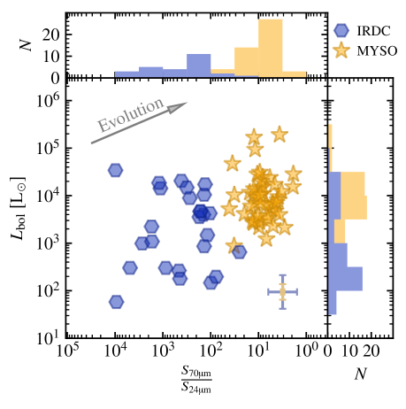
Figure 1: Mid-infrared, $S_{\mathrm{70{\rm\thinspace\upmu m}}}$ to $S_{\mathrm{24{\rm\thinspace\upmu m}}}$ flux ratios against bolometric luminosity for IRDC cores and MYSOs. The arrow represents the general evolutionary trend for an IRDC core through to an MYSO. Histograms of both mid-infrared ratios and bolometric luminosity are shown.

2.3 Distances, core masses, bolometric luminosities and infrared ratios

To ensure proper weighting of data-points during the employment of fitting algorithms, rather than use a typical error of $34\%$ for $\thinspace L_{\rm{bol}}$ (Mottram et al., 2011b), we instead recalculated $\delta\hbox{$\thinspace L_{\rm{bol}}$}$ for each target. To do this, standard errors were required for both bolometric flux and distance.

Bolometric fluxes and their errors were calculated by integrating the area under the infrared SED of each core of the IRDC subsample, for which a greybody function was used to fit to available infrared fluxes (see blue§ $3.2$ of Rathborne et al., 2010). In cases where the SED could not be reliably fit, bolometric fluxes were derived from the given luminosities/distances of Rathborne et al. (2010).

Core masses were calculated using Equation 1 (Hildebrand, 1983), with the same set of assumptions as used by Rathborne et al. (2006) (a dust opacity at $1.2\,\mathrm{mm}$, $\kappa_{\rm 1.2\,mm}=0.1\,\mathrm{cm^{2}\,g^{-1}}$ and dust-to-gas-mass ratio, $R=100$). Temperatures from our SED fits were used or, if not available, those derived by Rathborne et al. (2010). Our own distance estimates were also used (see below).

$$M_{\rm core}=\frac{R\,F_{1.2\,\rm mm}D^{2}}{\kappa_{\nu}B_{\nu}\left(T_{\rm dust}\right)}$$ (1)

where $R$ is the dust-to-gas-mass ratio, $F_{\mathrm{1.2\,mm}}$ is the core’s integrated flux at $1.2\,\mathrm{mm}$, $D$ is distance, $\kappa_{1.2\,\rm mm}$ is the dust opacity at $1.2\,\mathrm{mm}$ and $B_{\nu}\left(T_{\rm dust}\right)$ is the blackbody function.

Infrared flux ratios ($\nicefrac{{S_{70{\rm\thinspace\upmu m}}}}{{S_{24{\rm\thinspace\upmu m}}}}$) were derived from fitted SEDs. However, in some cases the measured $24{\rm\thinspace\upmu m}$ fluxes were not fit well by the greybody function and the ratio was instead calculated from the measured $24{\rm\thinspace\upmu m}$ flux and the $70{\rm\thinspace\upmu m}$ flux calculated from the greybody SED fit (which ignored flux measurements at $24{\rm\thinspace\upmu m}$) instead. For the MYSO sample, bolometric fluxes and their associated errors were taken from Mottram et al. (2011a), while $\nicefrac{{S_{70{\rm\thinspace\upmu m}}}}{{S_{24{\rm\thinspace\upmu m}}}}$ ratios were calculated using $S_{70{\rm\thinspace\upmu m}}$ and $S_{24{\rm\thinspace\upmu m}}$ values interpolated between IRAS, IGA, AKARI and/or WISE fluxes.

Distance errors were slightly more complex to quantify. While for distances determined via parallax measurements these errors are easily calculated, for those distances determined via kinematic analyses (i.e. the whole IRDC sample and most of the MYSO sample) another approach had to be used. A work by Wenger et al. (2018) used Monte Carlo techniques to determine kinematic distances, and their errors, to high-mass star formation regions in the Galaxy (their ‘Method C’), whose determined values were within a median difference of $14\%$ of those determined via parallax. To use this Monte Carlo technique, values for $v_{\mathrm{LSR}}$ were taken from Rathborne et al. (2006) and the RMS survey (Urquhart, J. S. et al., 2008). As a consistency check, distances calculated from this approach were compared to those derived using the alternate model of Reid et al. (2019). The two distances strongly agreed with eachother, with a mean/standard deviation of ${d_{\rm W18}}/{d_{\rm R19}}=1.05\pm 0.25$ where $d_{\rm W18}$ and $d_{\rm R19}$ are the distances computed via Wenger et al. (2018) and Reid et al. (2019), respectively.

It is important to note that although Mottram et al. (2011a) used previous kinematic distance estimates (with a general error of $\delta D=\pm 1{\rm\thinspace kpc}$) to determine extinction, and therefore $F_{\mathrm{bol}}$, the values derived for $F_{\mathrm{bol}}$ generally agreed for near/far kinematic distances (their Figure 2). Therefore using their values for $F_{\mathrm{bol}}$ should not significantly affect the estimates for $\thinspace L_{\rm{bol}}$ and $\delta\hbox{$\thinspace L_{\rm{bol}}$}$ presented in this work.

With these calculations of both bolometric fluxes and distances, as well as their errors, the calculation of bolometric luminosity and its error is a trivial exercise. Results for these are shown in Table 1 and Table 2 for the IRDC and MYSO sample respectively. It should be noted that for 26 of the 48 MYSOs we used more accurate distances from the literature (i.e. maser parallax measurements).

3 Observations

3.1 Observational information

All observations were taken with the Very Large Array (VLA) in its A-configuration, between 13^th October 2012 and 27^th December 2012 for $5.8{\rm\thinspace GHz}$ observations (project code 12B-140; PI - M. G. Hoare) and between 16^th March 2014 and 27^th July 2015 for $44{\rm\thinspace GHz}$ observations (project codes 14A-141 and 15A-238; PIs - S. L. Lumsden and S. J. D. Purser, respectively). The WIDAR correlator was set up in full continuum mode, with bandwidths of $2{\rm\thinspace GHz}$ ($16$ spectral windows of $64\times 2{\rm\thinspace MHz}$ channels with 8-bit samplers) and $8{\rm\thinspace GHz}$ ($64$ spectral windows of $64\times 2{\rm\thinspace MHz}$ channels with 3-bit samplers) centred on frequencies of $5.8$ and $44{\rm\thinspace GHz}$ respectively, which we refer to as C and Q-bands. In the A-configuration, the VLA has a minimum and maximum baseline length of $680\,\mathrm{m}$ and $36400\,\mathrm{m}$, corresponding to C and Q-band largest, recoverable, angular scales of $8\aas@@fstack{\prime\prime}9$ and $1\aas@@fstack{\prime\prime}2$ respectively. Synthesised beam widths of $\sim 0\aas@@fstack{\prime\prime}3$ and $\sim 0\aas@@fstack{\prime\prime}04$ are typical, while primary beam sizes at FWHM are $\sim 430\arcsec$ and $\sim 60\arcsec$.

In total, 56 target fields were observed at C-band and 49 fields at Q-band comprising observations of the 8 IRDCs and 48 MYSOs at both C and Q-bands, of which 38 were observed only at the lower frequency. Cores used as pointing centres for their IRDC complexes are denoted with an asterisk next to their name in Table 1. However, G033.69$-$00.01, which is a relatively extended complex, was observed at C-band with a pointing centre maximising the fraction of the IRDC in high-response areas of the primary beam ($\alpha_{\rm J2000}=18\hbox{$\rm{}^{h}$}52\hbox{$\rm{}^{m}$}54\aas@@fstack{s}0$ and $\delta_{\rm J2000}=00\degr 39\arcmin 39\arcsec$). At Q-band, the smaller primary beam necessitated a mosaic of 3 pointings with one pointing centre mirroring that at C-band, and the other two using coordinates of $\alpha_{\rm J2000}=18\hbox{$\rm{}^{h}$}52\hbox{$\rm{}^{m}$}49\aas@@fstack{s}9$, $\delta_{\rm J2000}=00\degr 37\arcmin 57\arcsec$ and $\alpha_{\rm J2000}18\hbox{$\rm{}^{h}$}52\hbox{$\rm{}^{m}$}58\aas@@fstack{s}1$, $\delta_{\rm J2000}=00\degr 41\arcmin 20\arcsec$. For the MYSO sample, the pointing centres are the coordinates of the MYSOs themselves as given in Table 2.

Depending on the LST of the observation, different flux and bandpass calibrators were used to bootstrap the flux density scale and calibrate the frequency-dependent gains. For calibration of the time-varying gains, a phase calibrator was observed every $12\min$ at C-band, for between $30-60{\rm\thinspace s}$ (dependent on calibrator flux). At Q-band, due to increased atmospheric instability, a calibrator cycle time of $2\min$, including slew times and phase-calibrator scan lengths ($30-40{\rm\thinspace s}$), was adopted. On-source times for the science targets were $24-26$ and $15-17\min$ achieving a theoretical rms noise of $6$ and $27{\rm\thinspace\upmu Jy}\,{\rm beam}^{-1}$ at C and Q-bands respectively. Target fields in the MYSO sample labelled between G$118$ and G$148$ only received half of the Q-band observing time required to achieve this sensitivity, resulting in a theoretical rms noise of $38{\rm\thinspace\upmu Jy}\,{\rm beam}^{-1}$. Synthesised beam sizes and rms noise levels achieved in the final images are shown in each plot (and caption) in blueFigures 15$-$71 of blueAppendix B.

For the flagging, editing, calibration and subsequent deconvolution/imaging, the casa software package (McMullin et al., 2007) was used in conjunction with the casa pipeline (version $4.7.2$). Manual flagging was performed first before running the pipeline, after which output calibration tables were manually inspected. In cases where erroneous calibration solutions were found, flagging was repeated and the pipeline was rerun until the time-varying gains, bandpass solutions and bootstrapped flux densities were of a high quality. At C-band, spectral cube imaging of the $2{\rm\thinspace MHz}$ ($\Delta v\sim 90\hbox{${\thinspace\rm{\rm\thinspace km}{\rm\thinspace s}^{-1}\,}$}$) channels corresponding to the $6.7{\rm\thinspace GHz}$ $\mathrm{CH}_{3}\mathrm{OH}$ maser line was conducted with maser positions recorded (green ‘$\,\times\,$’ in any contour plots) and the relevant channel(s) subsequently flagged prior to continuum imaging. Absolute position is accurate to within $10\%$ of the beam width, or $\sim 30{\rm\thinspace mas}$ at C-band and $\sim 4{\rm\thinspace mas}$ at Q. For all images primary-beam correction was applied.

Resulting imaging parameter, such as restoring beam dimensions, and image noise levels are summarised in LABEL:tab:BeamsNoises of Appendix A.

3.2 Performance of the array

An important diagnostic of collimated jets are spectral changes in flux and deconvolved major axis length. At different frequencies, Reynolds (1986) showed that the relative contributions of optically-thick and thin emission vary with a corresponding positional shift of the surface at which optical depth is unity (i.e. $\tau_{\nu}\sim 1$). These changes are quantified with the spectral indices $\alpha$ and $\gamma$ (whereby $\theta_{\rm maj}\left(\nu\right)\propto\nu^{\gamma}$ and $\theta_{\rm maj}$ is the observed jet length).

Unfortunately, when observing sources which may display extended emission, the degree to which different spatial scales are filtered out by interferometric observations is not well quantified for specific cases. With observational setups like those discussed above, where the same antenna configuration is used for radically different observing frequencies, this effect can be exacerbated. Since accurate spectral analysis is essential for radio jets we must therefore check if multi-frequency, A-configuration VLA-observing would significantly alter our measured values for $\alpha$ or $\gamma$.

To check the array performance of the VLA for our observations, the physical modelling, radiative-transfer and synthetic observation code, RaJePy (Purser, in prep) was used. A bi-conical jet profile (i.e. $\alpha=+0.6$ and $\gamma=-0.7$) with a mass-loss rate of $\hbox{$\dot{m}_{\rm jet}$}=5\times 10^{-6}\,\hbox{${\rm\thinspace M_{\odot}}$}{\rm\thinspace yr}^{-1}$, opening angle $\theta_{\rm op}=30\degr$ and distance of $D=3{\rm\thinspace kpc}$ was employed for the physical model which is representative of jets in general (P16). This profile was modelled up to an extent of $0\aas@@fstack{\prime\prime}5$ for both jet and counter-jet (total length of $1\arcsec$) using a cell size of $2{\rm\thinspace au}$ ($\sim 0.7{\rm\thinspace mas}$), ensuring good sampling of the flux distribution by the beam ($1\arcsec$ is $\sim 4$ C-band beams across). Synthetic observations were performed at each major frequency band of the VLA from L ($1-2{\rm\thinspace GHz}$) to Q-bands with A-configuration antenna positions and typical continuum bandwidths ($1-8{\rm\thinspace GHz}$).

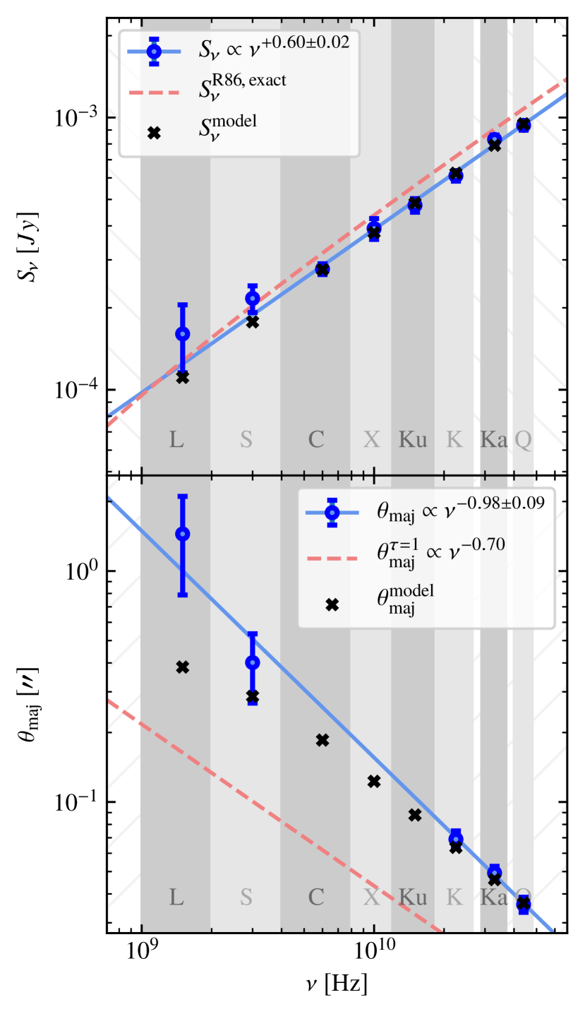
Figure 2: Performance of the A-configuration VLA towards a jet model with $\hbox{$\dot{m}_{\rm jet}$}=5\times 10^{-6}\,\hbox{${\rm\thinspace M_{\odot}}$}{\rm\thinspace yr}^{-1}$, $\theta_{\rm op}=30\degr$ and $D=3{\rm\thinspace kpc}$. Fluxes and deconvolved sizes derived from fitting a 2-D Gaussian in the image plane are shown in the top and bottom panels, respectively. Blue markers/errorbars show results for the synthetic observations, the LSQ fit to which is shown as a solid, blue line. Black, ’$\times$’ markers show the fit results towards the sky-model convolved with the restoring beams of the observations. Dashed, red curves show the flux predicted by Equation 8 of Reynolds (1986) (top panel) and the separation of the jet/counter-jet’s $\tau=1$ surfaces as given by their Equation 12. Observed bandwidths of each observing band are shown as shaded areas.

In Figure 2, the results of a single-component (Gaussian) fit to the recovered flux distributions of the synthetic observations are shown (blue points/errorbars). This fit failed at C, X and Ku-bands due to lower signal-to-noise, mixed with increasingly compact emission. For effective comparison, the same fit was performed on the sky model convolved with the clean beam of the observations (crosses). Recovered fluxes range from $98\pm 6\%-144\pm 40\%$ of the sky model’s showing them to be well-recovered by the VLA owing to the increasingly compact (with frequency) flux distribution and comprehensive $uv$-coverage of the array. A least-squares (LSQ) fit to the fluxes yields $\alpha=0.60\pm 0.02$, in good agreement with that expected from the analytical model of Reynolds (1986). From our synthetic observations the derived value of $\gamma=-1.0\pm 0.1$ diverges from $\gamma=-0.7$ expected for the $\tau=1$ surface from Reynolds (1986). We believe this results from approximating a jet’s flux distribution as a Gaussian, yet overall behaviour of $\theta_{\rm maj}$ is still a useful indicator that the extent of optically thick emission is contracting towards the jet-base with frequency.

For the purposes of this work, we find that the VLA in its A-configuration performs well towards science targets of this type. With insignificant levels of flux being lost due to spatial-filtering, spectral analysis of ionised jets from C/Q-band data such as that presented here is a useful diagnostic of physical conditions within the jets, and requires no baseline-matching between C and Q-bands.

4 Results

Every field was imaged out to $10\%$ of the primary beam’s peak response at each observed frequency ($\sim 6\arcmin$ and $\sim 1\arcmin$ from the pointing centre at C and Q-bands respectively) using a typical robustness of 0.5 and cell sizes of $0\aas@@fstack{\prime\prime}07$ and $0\aas@@fstack{\prime\prime}01$ respectively. blueAppendix B contains the resulting clean maps of radio flux in blueFigures 15$-$22 of blueAppendix B.1 for the IRDC sample and blueFigures 23$-$71 of blueAppendix B.2 for the MYSO sample. Links to each plot are available in LABEL:tab:BeamsNoises for ease.

For the measurement of fluxes and physical sizes, the same methods discussed in blue§$3.3$ of P16 were adopted (i.e. fitting of the emission with a Gaussian profile in the image plane). A full list of sources detected (i.e. $>5\upsigma$ where $\upsigma$ is the rms noise in each image) in the field are recorded, along with their derived fluxes and physical sizes, in blueTables LABEL:tab:CBandPosFlux$-$LABEL:tab:DeconvSizes. As a note, errors in flux used the local rms noise in their calculation, thereby accounting for the increased, effective noise towards the edge of the primary beam. Calculated spectral indices for both flux ($\alpha$) and deconvolved, major axis-length ($\gamma$), between $5.8{\rm\thinspace GHz}$ and $44{\rm\thinspace GHz}$, are recorded in LABEL:tab:AlphaGamma. At C-band, for the MYSO sample, only sources within $1\arcmin$ from the pointing centre are recorded (i.e. within the field imaged at Q-band, for spectral comparison). For reader ease, links to the discussion notes for each, individual object of both subsamples can be found in the last column of LABEL:tab:BeamsNoises. All clean images, data products and tables are also available online.

Classification of the compact radio sources follows the same algorithm discussed in blue§$\,4.1$ of P16. In light of the results of § 3.2 values for $\gamma$ are not restrictive (i.e. in that they must be related to $\alpha$ as per Reynolds, 1986) and only negative values are required for jets. Resulting classifications are summarised in Table 3, with a detailed breakdown in LABEL:tab:AlphaGamma. Detailed discussion of the classifications and results for each member of both samples are contained in blueAppendix D for the interested reader.

As a further note, we expect pollution of the sample by extragalactic sources to be minimal. An analysis of the radio catalogue of Bonaldi et al. (2019) shows that, within the C-band primary beam, we expect only 6 AGNs above a flux limit of $24{\rm\thinspace\upmu Jy}$ ($\sim 4\sigma$) and below a size-limit of $1\arcsec$ (and therefore of similar appearance to our targets of interest). At Q-band, due to the small primary beam and higher sensitivity limit, this number is negligible.

Table 3: Classifications of radio sources associated with each IRDC core (separated by core classification according to Rathborne et al., 2010) and MYSO. The final row indicates the number of cores/MYSOs associated with radio detections to those without. Classifications as a jet with a ‘C’ in parentheses indicates candidacy status as an ionised jet, while ‘L’ indicates association with shock-ionised lobes (see penultimate paragraph of § 1).

Type	IRDCs				MYSOs
	R	A	I	Q
Photo-ionised disc-wind	0	0	0	0	2
Hii region	5	0	1	0	3
Jet	1	0	0	0	3
Jet (C)	0	1	0	0	22
Jet (L)	0	0	0	0	10
Jet (L,C)	0	0	0	0	3
Unknown	1	0	0	0	2
Detection ratio	6:5	1:6	1:7	0:19	45:3

5 Analysis

5.1 IRDCs and their radio evolution

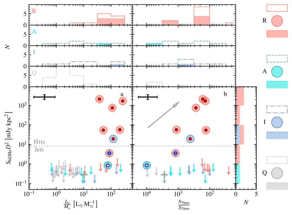
Figure 3: Plots of the $6{\rm\thinspace GHz}$ distance luminosities against parental core luminosity-to-mass ratios (panel a; data from Rathborne et al., 2010) and $70{\rm\thinspace\upmu m}$ to $24{\rm\thinspace\upmu m}$ flux ratios (panel b), for the IRDC sample. Cores harbouring radio-detections are shown as circles, the colour-scheme for which is based upon their classification (‘R’, ‘A’, ‘I’ or ‘Q’) according to Rathborne et al. (2010). Non-detections (upper limits) follow the same colour scheme based upon core classification. Smaller markers illustrate our radio source classification following the scheme of Figure 4 while the thick, ‘$+$’ marker denotes the IRDC cores coincident with detected CH₃OH masers. Histograms (colours as discussed) are shown, with solid bars showing cores with detected radio sources, while hollow bars include detections and radio non-detections. The dotted line delineates detected radio source classification from this work as Hii regions, or jets/jet candidates. Representative (median) errors are shown in the top left of each plot.

For their $1.2{\rm\thinspace mm}$-detected cores, Rathborne et al. (2010) employed the classification scheme of Chambers et al. (2009), as summarised in § 2.1. Based upon their infrared properties this scheme establishes a measure of the cores’ evolutionary states, from completely inactive (‘quiescent’) to harbouring active sites of star formation (‘red’). Exactly when a YSO jet’s radio emission ‘switches on’ during this evolution is an open question. Here we use both the core luminosity-to-mass and the $70{\rm\thinspace\upmu m}$ to $24{\rm\thinspace\upmu m}$ flux ratios as quantitative, evolutionary indicators. Both can be considered proxies for a core’s transition from a ‘cold’ (or quiescent) to a ‘hot’ (intermediate/active/red) molecular core and therefore age. In light of this and to investigate the onset of radio emission Figure 3 therefore plots detected radio flux against these indicators, showing that radio detections are only found towards some of the ‘I’, ‘A’ or ‘R’ cores whose luminosity-to-mass ratios are $\gtrsim 40$. No weak ($\gtrsim 30{\rm\thinspace\upmu Jy}\,{\rm beam}^{-1}$) radio emission is detected towards any quiescent (‘Q’) core (see Table 3 for a summary).

An intermediate-class core (MM2 of G024.60+00.08) displays maser emission yet no corresponding radio-continuum source is detected. Weak radio-continuum emission typical of ionised jets is seen towards the ‘R’ and ‘A’ cores G024.33+00.11 MM1 (the most massive of the sample) and G028.37+00.07 MM1 (which harbours two jet candidates), the most and third-most luminous cores within the sample. Those two cores harbouring jets also display maser emission, and their cores have higher luminosity-to-mass ratios than the maser-only source. Strong radio emission from Hii regions is observed towards six (five ‘R’ class and one ‘I’ class) cores possessing high $\nicefrac{{L_{\rm C}}}{{M_{\rm C}}}$ ratios. Those cores containing Hii regions also have higher values for $\nicefrac{{S_{70{\rm\thinspace\upmu m}}}}{{S_{24{\rm\thinspace\upmu m}}}}$ and radio flux (as expected), than those with jets (see panel b of Figure 3).

Evolutionarily, these findings make sequential sense. First, collapse-induced heating liberates volatile species into the gas phase via desorption from icy mantles (Viti et al., 2004), providing the conditions for maser emission from the desorbed CH₃OH. As the core collapses further, accretion and ejection phenomena in the form of discs and jets (the ‘Class I’ phase of low-mass star formation) produce weak radio emission, after which the newly formed massive protostar’s ultraviolet Lyman flux increases to the point whereby an Hii region is formed.

Due to the small number of radio sources detected towards the IRDC sample, only this brief analysis could be conducted. However those radio-detected IRDC cores harbouring jets and non-detections will help guide future surveys in terms of sensitivity requirements, especially in the SKA era.

5.2 Radio luminosity against bolometric luminosity

One of the key results of P16 was the segregation of MYSOs harbouring ionised jets from those powering Hii regions, in radio/bolometric luminosity parameter space. While the jets were found to occupy a region that adhered to the low-mass power-law for jets found by Anglada (1995), Hii regions were roughly as radio-luminous as their ultraviolet Lyman fluxes (inferred from the models of Davies et al., 2011) would predict. However there were some that were significantly lower than their predicted radio flux. These under-luminous Hii regions were still classified as such since classification was based on not just radio flux, but also upon morphology and infrared properties. This approach caught those Hii regions that were either resolved out by the interferometer and/or compact/optically-thick at the observed frequencies and is adopted in this work.

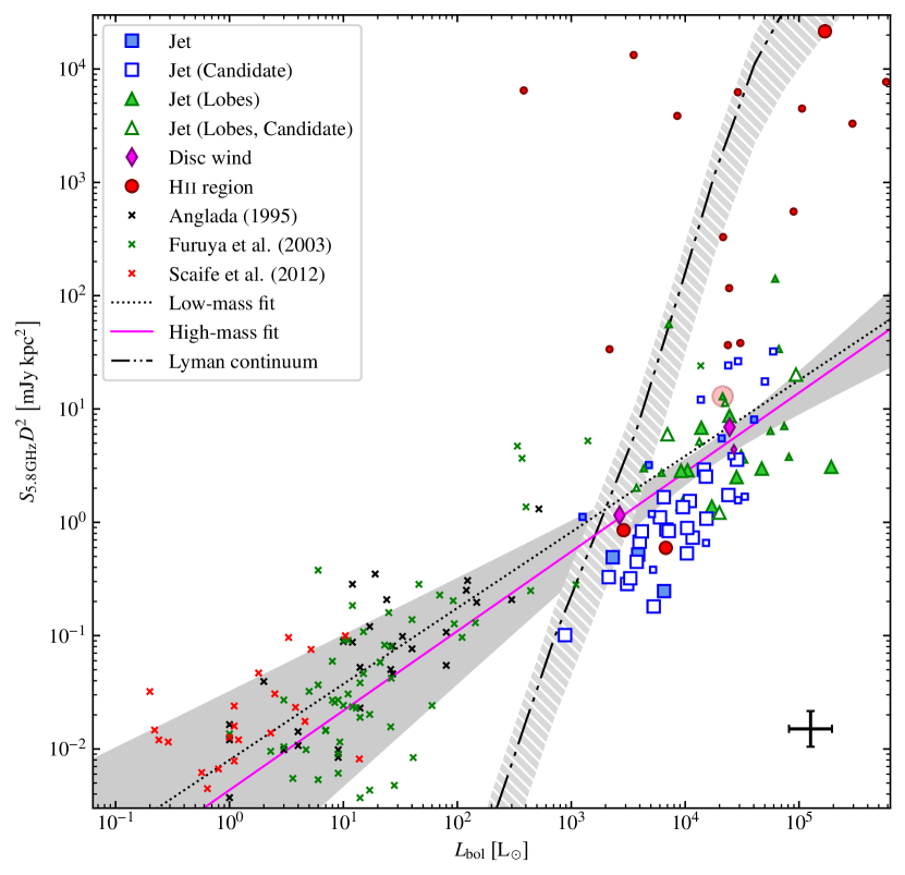
Figure 4: A plot of the radio luminosities at $5.8{\rm\thinspace GHz}$ against bolometric luminosity for those objects detected from the sample discussed in § 2.2. Different sub-classifications are marked as blue squares for jets, hollow blue squares for jet candidates, green triangles for jets with lobes, hollow green triangles for candidate jets with lobes, red circles for Hii regions and magenta diamonds for disc winds (see legend). Those objects from P16 are shown using the same scheme as discussed but half the marker size of the objects from this work. A contemporaneous jet/Hii region is highlighted by a red, transparent circle (G345.4938+01.4677, Guzmán et al., 2016). Note that for jets with lobes, only the central, thermal jet is plotted. Small ‘$\times$’ markers are low-mass radio jets, normalized to $5.8{\rm\thinspace GHz}$ (black, green and red for Anglada, 1995; Furuya et al., 2003; AMI Consortium et al., 2011, respectively), assuming $\alpha=0.6$ where the information is not available. The dotted line represents the power law we derived for the low-mass case (Equation 3), while the magenta line is that fitted to jets (not candidates) in this sample (Equation 2) with the $1\sigma$ confidence interval shaded in grey. Radio luminosity of an optically-thin, Hii region resulting from the ionising, ultraviolet, Lyman continuum of a ZAMS star of that $\thinspace L_{\rm{bol}}$ (calculated using the stellar models of Davies et al. (2011) for $\hbox{$\thinspace L_{\rm{bol}}$}>10^{3}\hbox{${\rm\thinspace L_{\odot}}$}$, and Thompson (1984) otherwise) is shown as a dot-dashed line. Lighter, grey, hatched shading represents the area where the radio-luminosity is between $20-180\%$ of that expected from those models. Representative (median) errors are shown in the bottom right of the plot.

To compare our results to those of P16, the C-band distance luminosities for the sample of P16 were calculated by using their derived values for spectral index. In cases identified as Hii regions where the loss of flux with increasing resolution becomes an issue (i.e. $\alpha_{\mathrm{measured}}<-0.1$), an optically thin spectral index is assumed and the flux at $5.8{\rm\thinspace GHz}$ is extrapolated from that measured at $5.5{\rm\thinspace GHz}$. In Figure 4, the calculated distance luminosities at $5.8{\rm\thinspace GHz}$ from P16 (smaller markers) are plotted against bolometric luminosity, as well as for all radio detections towards the MYSO sample of § 2.2 (larger markers). Fitting the jets (not candidates) from this work and those from P16 (whose $D$, $\thinspace L_{\rm{bol}}$ and $\delta\hbox{$\thinspace L_{\rm{bol}}$}$ were also recalculated using the methods of § 2.3) with a power law gives the relation shown as the magenta line in Figure 4 and explicitly stated in Equation 2. For this process the BCES algorithm of Akritas & Bershady (1996) was used since it takes into account errors in both $\thinspace L_{\rm{bol}}$ (independent variable) and $S_{\rm 5.8\,GHz}D^{2}$ (dependent variable). For comparison, we also fit the low-mass sample with the same algorithm, the results of which are plotted as a dotted line in Figure 4, and given in Equation 3. Both derived relations for low and high-mass YSOs agree within errors. This shows that jet radio luminosity scales with bolometric luminosity in the same way across 6 orders of magnitude, from $10^{-1}$ to $10^{6}\hbox{${\rm\thinspace L_{\odot}}$}$. As in P16, this suggests that those jets associated with high-mass MYSOs may be produced via ‘scaled-up’ processes of their lower-mass counterparts.

$$\log_{10}\left[\frac{S_{\rm 5.8{\rm\thinspace GHz}}D^{2}}{{\rm\thinspace mJy}\,{\rm\thinspace kpc}^{2}}\right] =(0.70\pm 0.24)\cdot\log_{10}\left[\frac{\hbox{$\thinspace L_{\rm{bol}}$}}{\hbox{${\rm\thinspace L_{\odot}}$}}\right]-(2.36\pm 1.02)$$ (2)

$$\log_{10}\left[\frac{S_{\rm 5.8{\rm\thinspace GHz}}D^{2}}{{\rm\thinspace mJy}\,{\rm\thinspace kpc}^{2}}\right] =(0.67\pm 0.06)\cdot\log_{10}\left[\frac{\hbox{$\thinspace L_{\rm{bol}}$}}{\hbox{${\rm\thinspace L_{\odot}}$}}\right]-(2.10\pm 0.07)$$ (3)

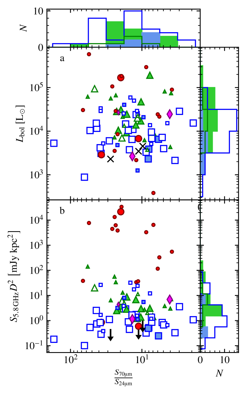
Figure 5: A plot of bolometric luminosity (panel a) and distance luminosity at $5.8{\rm\thinspace GHz}$ (panel b), against the $70{\rm\thinspace\upmu m}$ to $24{\rm\thinspace\upmu m}$ flux ratios. Black ‘$\times$’ symbols mark non-detections in panel a, which are consequently marked as upper limits in panel b. All other symbols have the same meaning as in Figure 4. Histograms are plotted for confirmed jets (solid bars) and candidate jets (line-only bars) using the same colour-scheme employed for the markers.

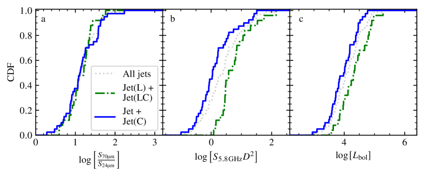
Figure 6: Calculated cumulative distribution functions for the $70{\rm\thinspace\upmu m}$ to $24{\rm\thinspace\upmu m}$ flux ratios (panel a), $5.8{\rm\thinspace GHz}$ radio luminosities (panel b) and bolometric luminosities of MYSOs harbouring ionised jets. CDFs for jets with lobes including candidate jets with lobes (dash-dotted green line), jets without lobes including candidates (solid blue line) and all jets and candidates (dotted grey line) are plotted.

5.3 Evolution and relationship of jets and shock-ionised lobes

Theoretical works have highlighted how accretion is a variable process. For example, Meyer et al. (2018) show how accretion rates increase in the first $\sim 10^{4}{\rm\thinspace yr}$ of an MYSO’s lifetime and how accretion rate variability becomes larger in amplitude towards the end of the MYSO stage. Due to the intrinsic connection between accretion and ejection, increased variability in the jet over time is expected. This may manifest itself at radio wavelengths as a time-varying radio flux for the thermal, radio jet, or an increase in the presence/change in the shock-ionised lobes along the jet’s axis due to evolving mass-loss characteristics (such as precession or varying ejection velocities). While the former requires multi-epoch observations to investigate, the latter can be examined by analysis of the shock-ionised lobes and their correlation to evolutionary indicators. With this in mind, we therefore investigate the jet sample and possible evolutionary trends connected to the presence of shock-ionised lobes below.

In Figure 5 the bolometric (panel a) and $5.8{\rm\thinspace GHz}$ distance luminosities (panel b) are plotted against the $70{\rm\thinspace\upmu m}/24{\rm\thinspace\upmu m}$ flux ratios. Superficially, those jets associated with lobes appear to occupy a narrower range of infrared flux ratios than those without lobes, with a mean/standard deviation for $\log_{10}(\nicefrac{{S_{70{\rm\thinspace\upmu m}}}}{{S_{24{\rm\thinspace\upmu m}}}})$ of $1.14\pm 0.29$ and $1.15\pm 0.40$, respectively. For the bolometric luminosity, the mean/standard deviation for $\log_{10}(\hbox{$\thinspace L_{\rm{bol}}$})$ is $4.34\pm 0.45$ and $3.96\pm 0.43$, while for the distance luminosity, $\log_{10}(S_{5.8{\rm\thinspace GHz}}D^{2})$ is $0.75\pm 0.50$ and $0.15\pm 0.60$ for the jets associated with lobes and those without, respectively. These statistics are reflected in the corresponding cumulative distribution functions (CDFs) plotted in Figure 6 and indicate that jets associated with lobes are found in a narrower range of infrared ratios, and at higher radio and bolometric luminosities.

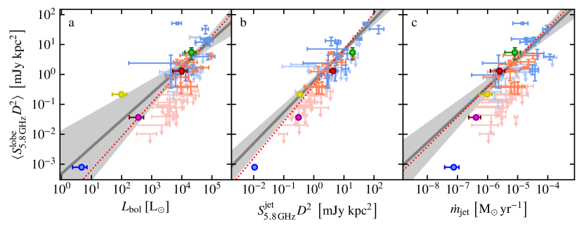
Figure 7: Log-mean $5.8{\rm\thinspace GHz}$ lobe luminosities against MYSO bolometric luminosity (panel a), central jet $5.8{\rm\thinspace GHz}$ luminosities (panel b) and central jet mass loss rates (panel c). Faded points represent $3\sigma$ upper limits on lobe luminosities for jets not associated with any lobes. Grey lines show the lines of best fit whose derived parameters are given in Table 4, with the $1\sigma$ confidence interval shaded light grey. Jet candidates, while plotted, are not included in this analysis. The red dotted line is the Akritas-Theil-Sen line (Akritas et al., 1995) which includes censored (i.e. upper-limits) data. Coloured circles represent YSOs from the literature for comparison which are, DG Tau A (blue marker; Purser et al., 2018), the Serpens triple radio source (yellow marker; Rodríguez-Kamenetzky et al., 2016), G035.02+0.35N (red marker; Sanna, A. et al., 2019), HOPS 370 (purple marker; Osorio et al., 2017) and HH 80-81 (green marker; Marti et al., 1993).

Table 4: Fitted power-law parameters (of the form $\log_{10}y=m\log_{10}x+c$), calculated partial correlation coefficients whilst controlling for distance ($\tau_{\rm kendall}^{xy.D}$) and their associated $p$-values. All fitted (not including upper limits) power-laws are represented in the relevant panels of Figure 7 as grey lines. For those fits not including upper-limits the BCES algorithm is used, otherwise the Akritas-Theil-Sen estimator (Akritas & Bershady, 1996) is used.

$x$	$y$	$N$	Include Upper limits?	$m$	$c$	$\tau^{xy.D}_{\rm kendall}$	$p$-value
$L_{\mathrm{bol}}$	$\langle S_{\mathrm{5.8\,GHz}}^{\mathrm{lobe}}D^{2}\rangle$	18	✗	$+0.90\pm 0.48$	$-3.33\pm 2.15$	$0.360$	$0.044$
			✓	$+1.13$	$-4.38$	$0.513$	$<0.001$
$S_{\mathrm{5.8\,GHz}}^{\mathrm{jet}}D^{2}$	$\langle S_{\mathrm{5.8\,GHz}}^{\mathrm{lobe}}D^{2}\rangle$	19	✗	$+1.04\pm 0.18$	$-0.23\pm 0.15$	$0.615$	$<0.001$
			✓	$+1.24$	$-0.40$	$0.658$	$<0.001$
$\dot{m}_{\mathrm{jet}}$	$\langle S_{\mathrm{5.8\,GHz}}^{\mathrm{lobe}}D^{2}\rangle$	19	✗	$+0.93\pm 0.30$	$+5.18\pm 1.51$	$0.485$	$0.005$
			✓	$+1.02$	$+5.67$	$0.558$	$<0.001$

To more thoroughly examine this conclusion two-sample, Kolmogrov-Smirnov (K-S) tests were performed to see if the jets with, and those without, lobes (for both our MYSO subsample and that of P16) were drawn from the same distributions in infrared flux ratios, radio luminosities and bolometric luminosities. K-S tests quantify this based upon a test statistic (values of $0\rightarrow 10$) and an associated $p$-value, defined as the probability of falsely rejecting the null hypothesis that both populations are drawn from the same distribution. For the mid-infrared ratios a K-S test statistic of $0.195$ and $p$-value of $0.537$ were calculated. For the radio luminosities these were calculated to be $0.580$ and $<0.001$, while for bolometric luminosity values of $0.330$ and $0.055$ were calculated respectively. Although this shows that the two samples could be drawn from the same mid-infrared ratio distribution and bolometric luminosity, the opposite is true for the radio luminosities.

To understand why shocked lobes are more prevalent towards brighter MYSOs, we compare lobe properties to those of the powering MYSO’s thermal jet. Therefore, in Figure 7, the log-mean (i.e. averaged over the lobes associated with each individual jet) $5.8{\rm\thinspace GHz}$ distance-luminosities for lobes associated with each jet from this work and those of P16 are plotted against bolometric luminosity (panel a), central jet luminosity (panel b) and jet mass loss rate (panel c; see § 5.5 for details on the calculation of $\dot{m}_{\rm jet}$). Upper limits ($3\sigma$) on lobe fluxes/luminosities for those jets without any associated lobes are also plotted. For the sample of P16, if no spectral indices were available (i.e. detection at only one frequency) extrapolation of lobe luminosities to $5.8{\rm\thinspace GHz}$ used an average value for spectral index of $\bar{\alpha}=-0.55\pm 0.31$ (as per the findings of P16). For all compared parameters, power-laws were fitted and, since all compared variables use distance in their respective calculations, partial correlation coefficients (controlling for distance) were calculated. Results for these are tabulated in Table 4 with fitted power-laws (using BCES as in § 5.2) also shown in Figure 7. From those results, we show a statistically-significant correlation of lobe luminosity with both jet luminosity and jet mass loss rate. No correlation between lobe and bolometric luminosity was found. For comparison, we also plot known examples of jets with lobes (HH 80-81, G35.2N, Serpens triple radio source, DG Tau A and HOPS 370) from the literature, across the YSO mass spectrum, as coloured circles in all panels of Figure 7. As can be seen, these objects adhere well to the derived power laws, regardless of their values for $\thinspace L_{\rm{bol}}$.

Interestingly, from panels b and c of Figure 7, the lobe-flux-density, $3\sigma$ upper-limits for jets without lobes appear to be lower than would be expected from their jets’ fluxes or mass loss rates. This may simply result from less luminous lobes falling below our sensitivity limits. Alternatively, jets with lower mass-loss rates may be less likely to produce lobes, implying a more intrinsic difference between them and higher-luminosity YSOs. In order to distinguish between these possibilities, we fit the lobe luminosities including both detections, as well as upper-limits of lobe luminosity for those jets without lobes. Since we are fitting singly-censored data (i.e. upper limits), the BCES algorithm is inadequate and instead the Akritas-Theil-Sen estimator (Akritas et al., 1995) is used, which is insensitive to outliers. Where this discrepancy is a detection issue, fitted parameters of these two algorithms should not change. As shown in Table 4, this is what is observed. When repeated for average lobe fluxes (i.e. not luminosity and therefore distance independent) against MYSO infrared flux and jet flux, the same result is seen. Thus, we establish that for the lower-luminosity radio jets, the non-detection of shock-ionised lobes is due to the sensitivity limit of our observations. Of course, this does not preclude the possibility that the lower-luminosity jets are less likely to produce lobes, a possibility which more sensitive radio observations are required to elicit.

5.4 Spectral indices and dust contribution

5.4.1 Thermal, protostellar radio emission

At cm-wavelengths emission from an MYSO is generally dominated by free-free emission from ionised gas. However, thermal emission from dust grains begins to dominate the spectral energy distribution in the mm-regime. At Q-band therefore, thermal dust emission may contribute to the measured flux. Fortunately, power-law contributions can be validly assumed for both the ionised and dust components since turnover frequencies of ionised jets are generally higher than $44{\rm\thinspace GHz}$ (from general consensus of observations) and mm-wavelengths fall under the Rayleigh-Jeans approximation ($h\nu\ll kT_{\rm dust}$). While the ionised jet’s flux follows a power-law, the dust’s flux is related to frequency by Equation 4 (where $\beta$ is the dust opacity index) with the total flux (ionised gas and dust) given in Equation 5. In the ISM, the average dust opacity index, $\beta$, is $\beta=1.8\pm 0.2$, while in protoplanetary discs, where grain agglomeration leads to increased dust grain sizes, this value can fall to $\beta\approx 1$ (Draine, 2006) or even less if observing an optically-thick, hot accretion-disc. Typically, for MYSOs the value for $\beta$ falls in the range $1\leq\beta\leq 2$ (e.g. $\beta=1$, $\beta=1.3$ and $\beta=1.5$ for Zhang et al., 2007; Galván-Madrid et al., 2010; Chen et al., 2016, respectively).

$$S_{\nu}^{\mathrm{dust}} \propto\nu^{\beta+2}$$ (4)

$$S_{\nu} =c_{1}\nu^{\alpha}+c_{2}\nu^{\beta+2}$$ (5)

where $c_{1}=S_{0}^{\mathrm{jet}}\nu_{0}^{-\alpha}$, $c_{2}=S_{0}^{\mathrm{dust}}\nu_{0}^{-\beta-2}$ and $S_{0}^{\mathrm{jet}}$ and $S_{0}^{\mathrm{dust}}$ are the flux contributions at some reference frequency, $\nu_{0}$, from the ionised and dust components respectively.

For establishing dust contributions to the Q-band fluxes we employ four methods which are listed, and subsequently discussed, below:

1. Interpolation of $S_{\rm 44{\rm\thinspace GHz}}$ using matching-resolution mm/sub-mm observations

2. Extrapolation of $S_{\rm 44{\rm\thinspace GHz}}$ using fluxes from L to Ka-bands

3. Analysis of position angle differences from C to Q-band

4. Comparison of spectral index distribution across the sample with that of ‘dust-free’ surveys

Method 1: Matching-resolution, sub-mm/mm fluxes are available in only two cases, G160.1452+03.1559 and G173.4815+02.4459 (within the field of view for G173.4839+02.4317). For each of those two MYSOs, it is therefore possible to constrain the SED of the central, thermal source and directly derive the power-laws governing dust and ionised emission. Using the method of least squares in conjunction with Equation 5 we deduce that dust contributes $22\pm 9\%$ of the Q-band flux for G160.1452+03.1559 and $1\pm 4\%$ for G173.4815+02.4459. Further details are available in § D.2.40 and § D.2.41 of blueAppendix D, respectively.

Method 2: In Figure 8, five MYSOs’ radio SEDs are plotted which include cm-fluxes from four other surveys. Using the method of least squares a power-law was fitted to those fluxes recorded at frequencies ranging from $1.5-25.5{\rm\thinspace GHz}$ (where dust emission is assumed to be negligible), with derived values for $\alpha$ indicated on each panel. From those power-laws the predicted, dust-free Q-band flux was calculated (errors are the prediction interval) along with its difference with the observed flux, $\Delta S_{\rm Q}$ (also indicated in each panel). Values in the range $-21\pm 24\%\leq\Delta S_{\rm Q}\leq+46\pm 69\%$ show that, within errors, no excess flux from dust is therefore observed in these examples.

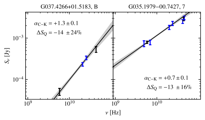
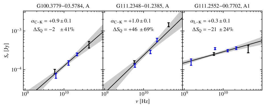
Figure 8: Radio SEDs for the thermal radio emission of 5 MYSOs in our sample, including fluxes taken from the literature (blue error-bars). Spectral indices derived from fluxes between L and K-bands are indicated, as well as the excess Q-band flux, $\Delta S_{\rm Q}$. Grey shading indicates the $1\sigma$ confidence intervals on the power-laws derived (solid, black lines). References: Top row, left panel - Rosero et al. (2016). Top row, right panel - Rosero et al. (2019) for component 7 of G035.1979–00.7427 Bottom row - Sanna, A. et al. (2018) and Obonyo et al. (2019) (L-band flux of G111.2552–00.7702). In the case of component A1 of G111.2552–00.7702, the C-band flux recorded by Sanna, A. et al. (2018) is disregarded in the power-law fit due to source confusion.

Method 3: Across our sample, 13 MYSOs with jet-like emission were measured to have finite, deconvolved sizes at both C and Q-bands. In those examples the difference in major-axis position angles, $|\theta_{\rm PA}^{\rm C}-\theta_{\rm PA}^{\rm Q}|$, could therefore be calculated. It is expected that $|\theta_{\rm PA}^{\rm C}-\theta_{\rm PA}^{\rm Q}|=0\degr$ if jet-emission dominates and $|\theta_{\rm PA}^{\rm C}-\theta_{\rm PA}^{\rm Q}|=90\degr$ when dust-contributions dominate. Between these two values, both the jet and dust contribute significant emission. In Figure 9, we therefore plot the histogram for $|\theta_{\rm PA}^{\rm C}-\theta_{\rm PA}^{\rm Q}|$ showing that jet-emission dominates in most cases. To quantify the average fraction of the Q-band flux from dust emission, we have fitted this histogram with two Gaussian distributions whose means are fixed at $0\degr$ and $90\degr$ (solid, black line in Figure 9). Using the ratio of the areas under each distribution as a proxy for relative flux contributions, we estimate that dust contributes an average of $29\pm 23\%$ to the Q-band fluxes across our sample.

Figure 9: Histogram of differences in major axis position angle from C to Q-band across the sample. Binning is defined as $s+w(n-1)\leq\alpha<s+wn$, where $s$ is the left edge value for the left-most bin ($|\theta_{\rm PA}^{\rm C}-\theta_{\rm PA}^{\rm Q}|=0\degr$), $n$ is the bin number (starting at $1$ with the left-hand bin) and $w$ is the bin width ($15\degr$). The black line shows the fit of a double-Gaussian distribution to the histogram.

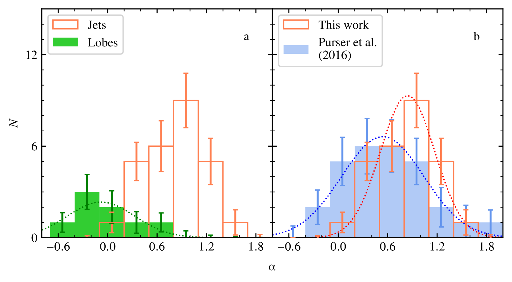
Figure 10: Histograms of spectral indices for: a.) All lobes (green) and jet-like sources (red) for which a spectral index between C and Q-bands was derived. b.) All jet-like sources with a derived spectral index from this work (red) and those from P16 (blue). Normal distributions have been fitted to the jets from this work (red dotted line) and from P16 (blue dotted line). Binning is defined as $s+w(n-1)\leq\alpha<s+wn$, where $s$ is the left edge value for the left-most bin ($\alpha=-0.7$), $n$ is the bin number (starting at $1$ with the left-hand bin) and $w$ is the bin width ($0.2$ for panel a and $0.3$ for panel b).

Method 4: Histograms of the spectral indices found towards the ionised jets (Figure 10) were compared to those of the lower frequency ($\nu_{\rm obs}<23{\rm\thinspace GHz}$) survey of P16 (their Figure 7), where sources have a minimal dust contribution. The resulting histograms are plotted in Figure 10. Comparison between spectral indices recorded in P16 and those here shows that those jets observed in this work tend to have higher values for $\alpha$ than those of P16. Fitting a normal distribution to each sample yields a mean spectral index of $\bar{\alpha}_{\mathrm{P16}}=0.54$ and $\bar{\alpha}_{\mathrm{VLA}}=0.84$ (this work) for the jets from P16 andt his work, respectively. Due to the use of the same classification scheme, there should be no intrinsic differences between southern and northern hemisphere jets and this difference is therefore attributable to dust contributions at Q-band which increase the derived values for $\bar{\alpha}$. Using the derived values for $\bar{\alpha}$, dust therefore contributes an average of $46\pm 10\%$ of the total emission at Q-band, across our sample. This value is similar to the results of method 3 and to values obtained by Sánchez-Monge et al. (2008). In that work 2 of a sample of 4 MYSOs showed dust contributions to the Q-band flux of $38\%$ and $44\%$ for IRAS 04579+4703 (our G160.1452+03.1559; see § D.2.40) and IRAS 22198+6336, respectively.

Considering the results of each method outlined above, dust contributions do not dominate at Q-band. However, measurable changes in the average spectral index and changes in the deconvolved position angles from C to Q-bands are observed showing dust still contributes. Considering method 4 had the largest sample sizes of any of the methods, we therefore conclude that within our sample dust contributes an average of $44\pm 10\%$ of the Q-band flux. Individual contributions can not be discerned at this point however, and therefore recorded spectral indices are not adjusted.

As a note, we also investigated the relationship between $|\theta_{\rm PA}^{\rm C}-\theta_{\rm PA}^{\rm Q}|$ and $\alpha$, as we would expect higher values of $\alpha$ in cases of increased dust contributions, however no correlation was observed.

5.4.2 Shock-ionised lobes

As for the shock-ionised lobes’ spectral index distribution, the population with detections at both C and Q-bands, and therefore with calculated values for $\alpha$ between these frequencies, is relatively small (4 lobes). An L-band survey by Obonyo et al. (2019) observed some of our sample’s sources and, in conjunction with our results, derived spectral indices for some of the associated lobes. These have been included along with ours and plotted as a histogram in panel (a) of Figure 10 (green bars). Subsequently we calculate that the associated lobes (4 from this work and 4 from Obonyo et al., 2019) belong to a normal distribution with a mean value of $\bar{\alpha}=-0.08$ and standard deviation of $\sigma_{\alpha}=0.41$ (green, dotted line in panel a of Figure 10), much flatter than the average spectral index found by P16 ($\bar{\alpha}=-0.55$). We believe that this results from several factors (1) only lobes with shallower spectral indices would be detected in this work, (2) shock-ionised lobes have $\alpha\sim-0.5$ (P16), lowering their signal-to-noise at Q-band (3) Shock-ionised lobes are extended on the arcsecond-scale and therefore flux-loss at Q-band is an issue. Due to these observational selection effects, as well as small sample size, no further analysis was performed.

5.5 Mass loss and accretion

Jets’ mass loss rates are an important parameter which can act as a discriminator between different jet-launching mechanisms. When compared with accretion rates (using the so called, ‘magnetic lever arm’ parameter, $\lambda=\nicefrac{{\dot{m}_{\rm acc}}}{{\hbox{$\dot{m}_{\rm jet}$}}}$; Frank et al., 2014) we can discriminate between different magneto-centrifugal launching mechanisms. Whilst ‘X-winds’ typically are expected to have $\nicefrac{{1}}{{\lambda}}\sim 0.3$ (Shu & Shang, 1997), values of $\nicefrac{{1}}{{\lambda}}\sim 0.1$ are anticipated for the disk-winds described by Pelletier & Pudritz (1992). Radiative launching mechanisms have also been suggested and we can determine their significance by comparing $\dot{m}_{\rm jet}$ with $\thinspace L_{\rm{bol}}$ since for radiatively-launched/line-driven jets $\hbox{$\dot{m}_{\rm jet}$}\propto\hbox{$\thinspace L_{\rm{bol}}$}^{\nicefrac{{3}}{{2}}}$ (Proga et al., 1998).

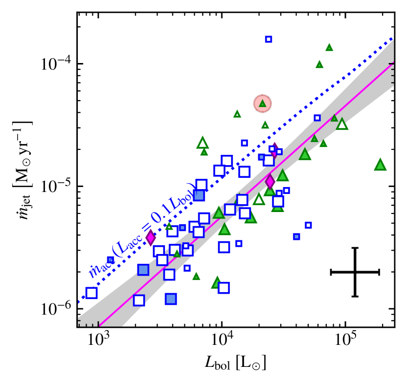
Figure 11: A plot of the jet mass loss rate against bolometric luminosity for jet-like sources detected. Symbols have the same meaning as in Figure 4 and the magenta line is the fit (Equation 6) to both the data presented here and that of P16 with the corresponding $1\sigma$ confidence interval shaded in light grey. The dotted line represents the accretion rate (using Equation 7 and assuming $L_{\rm acc}=0.1\hbox{$\thinspace L_{\rm{bol}}$}$, Cooper et al., 2013).

For this work one of two techniques was used to compute $\dot{m}_{\rm jet}$ based upon the observed values for $\alpha$ (details of which are can be found in blueAppendix C). Calculated values for $\dot{m}_{\rm jet}$ possess a range from $(1.2\pm 0.7)\times 10^{-6}$ to $(1.8\pm 0.4)\times 10^{-5}\hbox{${\rm\thinspace M_{\odot}}$}{\rm\thinspace yr}^{-1}$, a mean (of log values) of $(8.7\pm 6.1)\times 10^{-6}\hbox{${\rm\thinspace M_{\odot}}$}{\rm\thinspace yr}^{-1}$ and a median of $\left(6.1\pm 2.5\right)\times 10^{-6}\hbox{${\rm\thinspace M_{\odot}}$}{\rm\thinspace yr}^{-1}$. A full table of calculated values of $\dot{m}_{\rm jet}$ for each individual case is available in LABEL:tab:JMLsOpangs of blueAppendix A. In Figure 11 we have plotted $\dot{m}_{\rm jet}$ against $\thinspace L_{\rm{bol}}$ for all jets from our sample and those from P16. A power-law was fitted to the sample of this work and that of P16, not including candidates, using the same methods discussed in § 5.2. Consequently, Equation 6 shows the derived relation for the combined sample which is plotted as a solid, magenta line in Figure 11. For this relation we derive a partial correlation coefficient, whilst controlling for distance, of $\tau_{\rm kendall}=0.554$ with an associated $p$-value of $\sim 1\times 10^{-4}$ showing a significant correlation between $\dot{m}_{\rm jet}$ and $\thinspace L_{\rm{bol}}$.

$$\log_{10}\left[\frac{\hbox{$\dot{m}_{\rm jet}$}}{\hbox{${\rm\thinspace M_{\odot}}$}{\rm\thinspace yr}^{-1}}\right] =(0.90\pm 0.19)\cdot\log_{10}\left[\frac{\hbox{$\thinspace L_{\rm{bol}}$}}{\hbox{${\rm\thinspace L_{\odot}}$}}\right]-(8.85\pm 0.78)$$ (6)

As discussed above, jets are proposed to be launched magnetocentrifugally or radiative line-driving. For the latter, it is expected that $\hbox{$\dot{m}_{\rm jet}$}\propto\hbox{$\thinspace L_{\rm{bol}}$}^{\nicefrac{{3}}{{2}}}$ (Proga et al., 1998) yet we find that $\hbox{$\dot{m}_{\rm jet}$}\propto\hbox{$\thinspace L_{\rm{bol}}$}^{0.90\pm 0.19}$. We take this as evidence negating line-driving as the dominant launching mechanism of jets from MYSOs.

To discern between competing magnetocentrifugal mechanisms, establishing the ratio of accretion to ejection rates is of paramount importance. Using Equation 7, accretion rates were calculated from the accretion luminosities (whereby $\nicefrac{{L_{\mathrm{acc}}}}{{L_{\mathrm{bol}}}}=0.1$) following the work of Cooper et al. (2013) who assumed the empirical relationship between Br$\gamma$ and accretion luminosity (see their Figure 8). For that calculation, the results of Davies et al. (2011) were used to compute $R_{\star}$ and $M_{\mathrm{\star}}$ assuming the ZAMS configuration can approximate the MYSOs’ protostellar structure.

$$\dot{m}_{\mathrm{acc}}=\frac{R_{\star}L_{\mathrm{{acc}}}}{\mathrm{G}M_{\star}}$$ (7)

where $\dot{m}_{\rm acc}$ is the accretion rate, $R_{\star}$ is the radius of the MYSO, $L_{\rm acc}$ is the accretion luminosity and $M_{\star}$ is the mass of the MYSO.

In Figure 11 the accretion rate is shown (blue, dotted line) and compared to our correlation for the jets’ mass loss rates suggesting a reasonably constant ratio of $\nicefrac{{\hbox{$\dot{m}_{\rm jet}$}}}{{\dot{m}_{\mathrm{acc}}}}$ across the high-mass regime. Finding the ratios of calculated values for $\dot{m}_{\rm jet}$ and $\dot{m}_{\rm acc}$ gives an average value for $\nicefrac{{\hbox{$\dot{m}_{\rm jet}$}}}{{\dot{m}_{\mathrm{acc}}}}$ of $0.19$ with a standard deviation of $0.19$, higher than those found towards low mass cases ($\sim 0.01-0.1$; Hartigan et al., 1994). However, due to the large approximations involved in the calculations of $\dot{m}_{\rm jet}$ and $\dot{m}_{\rm acc}$, determining the dominant model of jet launching in MYSOs can not be achieved from the results here. To constrain the models further, a more accurate follow-up survey to constrain the accretion rates of each object, as well as jet velocities and ionisation fractions, is required to definitively measure this ratio.

5.6 Jets and molecular outflows

How molecular outflows are driven is as yet unknown, with a possibility being entrainment by jets. Guzmán et al. (2012) argued that the typical momenta of jets, when compared with that of the large scale outflows, was too small to drive them. On the other hand, Sanna et al. (2016) showed that the ratio between the momentum of a $4\times 10^{4}\hbox{${\rm\thinspace L_{\odot}}$}$ MYSO’s jet and that of its associated molecular outflow, over the dynamical timescale of the outflow, was of order unity. This indicated that the jet was mechanically able to fully drive the outflow. Since this was a single object study, its application to MYSOs and their molecular outflows in general necessitates a larger sample.

A distance-limited survey of 89 MYSOs by Maud et al. (2015) showed 59 to be associated with massive, molecular outflows and derived relationships for outflow force and momentum with $\thinspace L_{\rm{bol}}$ (their Table 6). Consequently they also established an average dynamical timescale ($\bar{t}_{\rm dyn}$) for the molecular outflows of $8.4\times 10^{4}{\rm\thinspace yr}$, roughly the same as known timescales for massive star formation ($\sim 10^{5}{\rm\thinspace yr}$, McKee & Tan, 2003; Mottram et al., 2011b). Combining the work presented here with that of P16, an opportunity to compare the momenta of the molecular outflows (from Maud et al., 2015) and jets is available.

To calculate the momenta of the jets, their force (i.e. momentum rate), $F_{\rm jet}$, which is the product of jet velocity and mass loss rate, is integrated over time. Assuming $v_{\rm jet}=500\hbox{${\thinspace\rm{\rm\thinspace km}{\rm\thinspace s}^{-1}\,}$}$ and a jet lifetime of $8.4\times 10^{4}{\rm\thinspace yr}$ (i.e. $\bar{t}_{\rm dyn}$ of the molecular outflows), we calculate the total momenta of the jets, $p_{\rm jet}$. In Figure 12 $p_{\rm jet}$ is plotted against $\thinspace L_{\rm{bol}}$ with the relationship for the molecular outflows from Maud et al. (2015) also shown (blue dotted line). Taking the ratio of these two power-laws, as with the single object study of Sanna et al. (2016), $\nicefrac{{p_{\rm jet}}}{{p_{\rm outflow}}}\gtrsim 1$ ($0.9-2.1$ in the range $10^{3}\leq L_{\rm bol}\leq 10^{5}$), supporting the idea that jets are the driving forces behind the molecular outflows. To further investigate this result, proper motion studies should be utilised to calculate jet velocities, and therefore total momentum, more accurately.

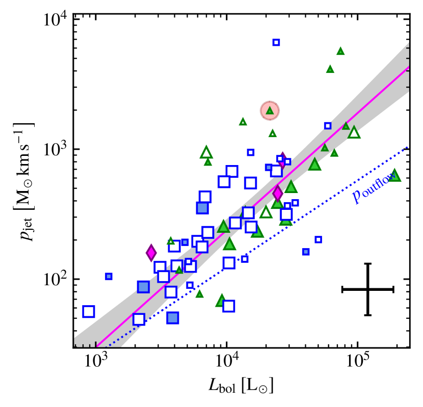
Figure 12: A plot of the total jet momentum against bolometric luminosity. Symbols have the same meaning as in Figure 4, while the magenta line is the fit to both the data presented here and that of P16 with the $1\sigma$ confidence interval shaded in light grey. The dotted line is the relationship between $p_{\mathrm{outflow}}$ and $\thinspace L_{\rm{bol}}$ from Table 6 of Maud et al. (2015).

5.7 Measured sizes and implications

Early expansion of Hii regions may be governed by the interplay between pressure outwards and gravitational forces inwards (Keto, 2002). Towards more-evolved Hii regions, the gas pressure far exceeds the gravitational forces (i.e. $\tfrac{GM^{2}}{rnkT}\ll 1$) at their Strömgren radii where ionisation is halted due to equality of Lyman fluxes and recombination rates. However, an MYSO with limited UV photon flux has a much smaller Strömgren radius, whereby $\tfrac{GM^{2}}{rnkT}\gg 1$, and therefore the Hii region can become trapped only to expand when its radius exceeds that of the ‘gravitational radius’, $r_{\rm g}$ (Equation 8).

$$r_{\rm g}=\frac{GM_{\star}}{{2v_{\mathrm{s}}}^{2}}$$ (8)

where $M_{\star}$ is the MYSO mass and $v_{\mathrm{s}}$ is the sound speed ($v_{\mathrm{s}}=\sqrt{\tfrac{kT}{m_{\rm H}}}$ where $T\sim 10^{4}{\rm\thinspace K}$ and $m_{\rm H}$ is the mass of hydrogen).

Pertinent to this work, these lines of thought lead to the question of whether observed thermal, free-free, radio emission originates in a trapped Hii region, or an ionised jet. To differentiate between the two possibilities, the gravitational radius of the MYSO and physical extent of the ionised gas must be compared, with similarity between the two quantities favouring a trapped Hii region. It is possible to infer MYSO mass from bolometric luminosity using the models of Davies et al. (2011), and therefore calculate gravitational radius using Equation 8. A measure of the plasma’s physical extent can be deduced from the radio images, assuming the radio component can be reasonably described by a 2-D Gaussian function.

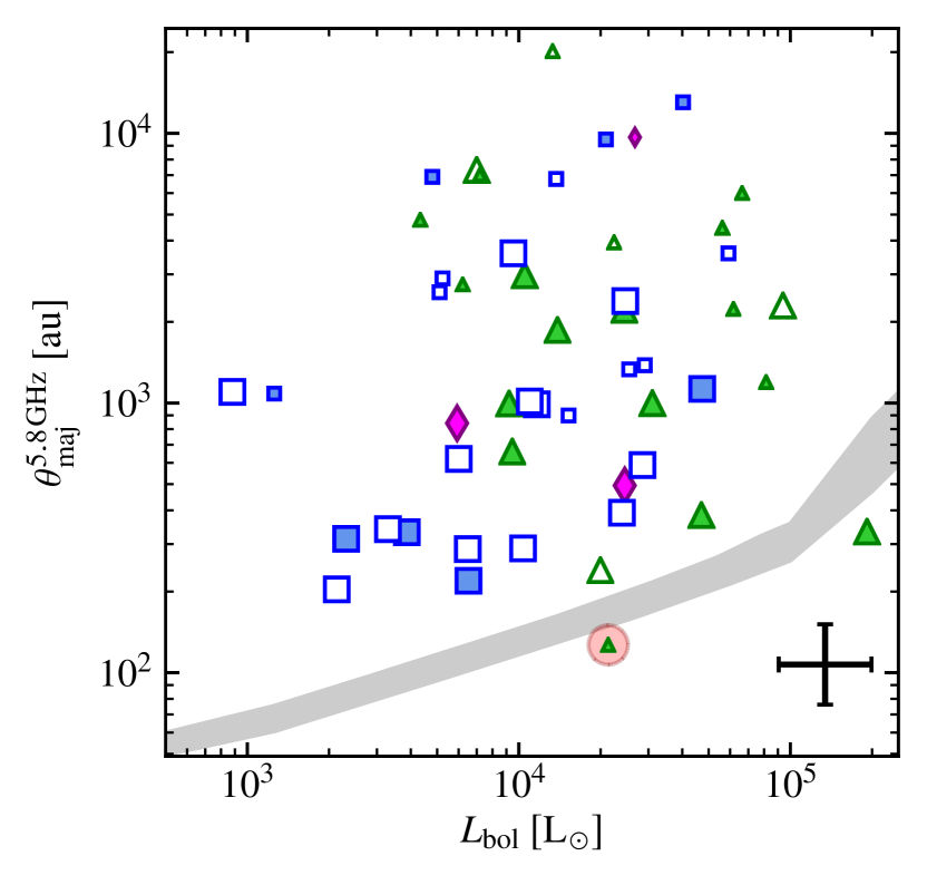
Figure 13: Deconvolved major axis length at $5.8{\rm\thinspace GHz}$, as derived using imfit, against bolometric luminosity for all sources displaying jet-like characteristics. Symbols are the same as in Figure 4, while the grey area represents twice the gravitational radius (Equation 8) for the relevant bolometric luminosity, with a $34\%$ error, (Davies et al., 2011).

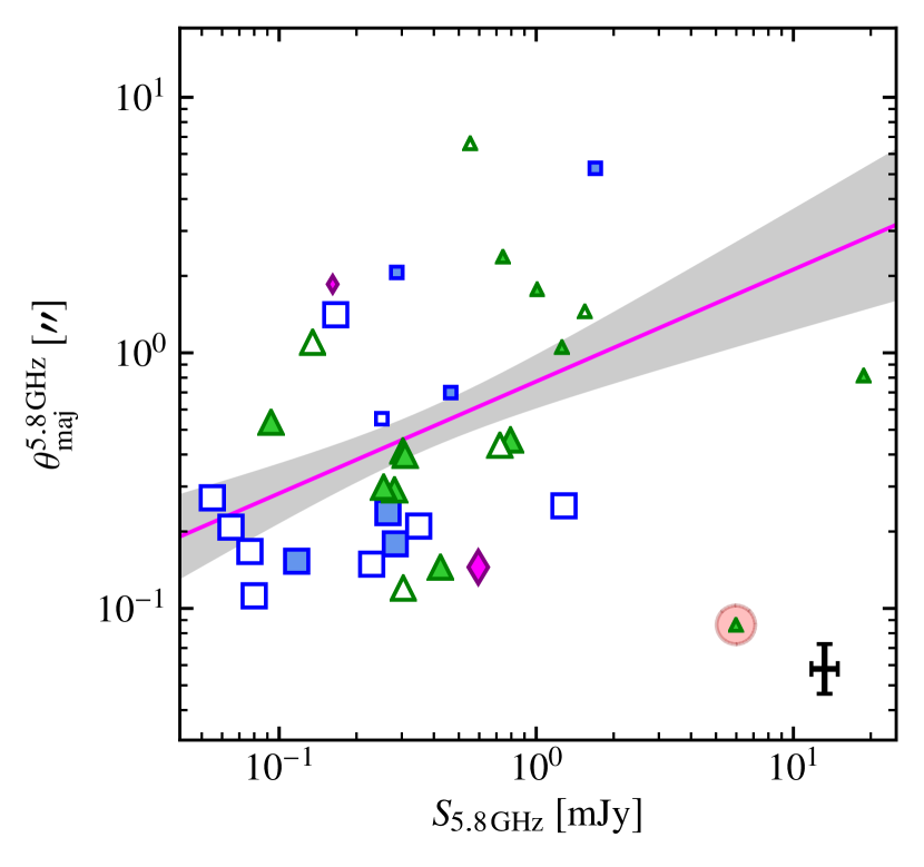
Figure 14: Deconvolved major axis length at $5.8{\rm\thinspace GHz}$ (in arcseconds), as derived using imfit, against radio flux at $5.8{\rm\thinspace GHz}$ for all sources displaying jet-like characteristics. Our fit (Equation 10) to both the jet-like sources of this work and those of P16 is shown as a magenta line with the fit’s $1\sigma$ confidence interval shaded light grey. All markers used are the same as in Figure 4.

In Figure 13, the deduced major axes are plotted against bolometric luminosity for all sources with jet-like characteristics. Also plotted are the expected gravitational radii calculated using Equation 8 in conjunction with the models of Davies et al. (2011). In cases where measurement of $\theta_{\rm maj}$ was only possible at one frequency, a standard value of $\gamma=-0.7$ was used to extrapolate to $5.8{\rm\thinspace GHz}$. No relation between jet major axis length and bolometric luminosity is found with a partial $\tau_{\rm kendall}$ (whilst controlling for distance) of 0.026 and corresponding $p$-value of 0.796. It is apparent that the major axes far exceed the gravitational radii. From Keto (2002), the ionisation front of an expanding Hii region moves with an approximate velocity of $\sim 5\hbox{${\thinspace\rm{\rm\thinspace km}{\rm\thinspace s}^{-1}\,}$}$, corresponding to mean and median dynamical times for the ionisation front of $\sim 640{\rm\thinspace yr}$ and $1000{\rm\thinspace yr}$ respectively. Considering the whole process of massive star formation is thought to last $\sim 10^{5}{\rm\thinspace yr}$ (Davies et al., 2011), only a small percentage of the jet-candidates observed could potentially be recently untrapped Hii regions, while the vast majority must have an elongated, ionised jet component to explain the large extent over which ionised material is found. As a further note, it is interesting that the contemporaneous Hii/jet from P16, G345.4938+01.4677, has a major axis length which coincides with that expected of a trapped Hii region model (highlighted marker in Figure 13).

Another question, that an analysis of jet morphology may answer, is that of jet collimation and on what scales it typically occurs. From Equations 12 and 16 of Reynolds (1986) it can be shown that

$$\left[\frac{\theta_{\rm maj}}{{\rm\thinspace au}}\right] \propto\left(S_{\nu}D^{2}\right)^{\frac{1}{1+\epsilon+q_{\rm T}}}$$

$$\Rightarrow\left[\frac{\theta_{\rm maj}}{\prime\prime}\right] \propto S_{\nu}^{\frac{1}{1+\epsilon+q_{\rm T}}}D^{\frac{2}{1+\epsilon+q_{\rm T}}-1}$$ (9)

where $\epsilon$ is the power-law coefficient for variation of jet-width along its length, and $q_{\rm T}$ is a similar coefficient for temperature. In sensible physical models of jets, these parameters are constrained to be $0\leq\epsilon\leq 1$ and $q_{\rm T}\leq 0$.

For the standard, non-recombining, conical jet model whereby the jet material adheres to ballistic trajectories (i.e. no longer influenced by magnetic fields), $\epsilon=1$ and $q_{\rm T}=0$. If the conical model were the dominant model to generally describe the jets in our sample, it is expected that $\theta_{\rm maj}\propto S_{\nu}^{\nicefrac{{1}}{{2}}}$ following from Equation 9. Whereas for jets still under collimation, we would expect $\epsilon<1$ and therefore a steeper relation since $\left(1+\epsilon+q_{\rm T}\right)^{-1}>\nicefrac{{1}}{{2}}$ (assuming significant cooling does not occur on these scales).

$$\log_{10}\left[\frac{\theta_{\rm maj}}{\prime\prime}\right] =(0.44\pm 0.16)\cdot\log_{10}\left[\frac{S_{\rm 5.8{\rm\thinspace GHz}}}{{\rm\thinspace mJy}}\right]-(0.11\pm 0.12)$$ (10)

In Figure 14 therefore, we examine major axis length and its relationship with radio flux at $5.8{\rm\thinspace GHz}$ (to avoid emission from dust at Q-band). A power law is fitted to ascertain the dominant jet model, the results of which are given in Equation 10. Since we find a power-law coefficient of $0.44\pm 0.16$ and following from the above discussion, this may be evidence showing that the standard, conical model for ionised jets is the dominant one on the scales probed by our observations ($\sim 10^{2}-10^{4}{\rm\thinspace au}$). However, we calculate a partial $\tau_{\rm kendall}$ (whilst controlling for distance) of 0.337 and corresponding $p$-value of 0.009, which hints at the presence of correlation but is not conclusive (i.e. $p<0.001$). Possible inaccuracies in the measurement of $\theta_{\rm maj}$ resulting from deconvolution errors or non-constant mass ejection may have affected the quality of results. Further, more sensitive and multi-epoch radio observations would be therefore be required to more thoroughly establish, or dismiss, the tentative relationship seen above.

6 Summary and Conclusions

Presented here, our radio observations towards forming massive stars at a variety of evolutionary stages represents the largest radio survey of jets associated with massive protostars to date. It has resulted in the detection of 14 (confirmed) ionised jets coincident with the MYSOs’ infrared positions, of which 10 are determined to be associated with shock-ionised, radio lobes. Including those radio sources which hold jet-candidacy status this increases to a total of 38. Within $60\arcsec$ of the pointing centres and linked to other sites of star formation, a further 22 jets or candidates (6 of which are associated with lobes) are found. Analysis of the radio properties of this new, northern-hemisphere sample of ionised jets, as well as that from P16, were conducted to determine ionised jets’ role in massive star formation, as well as their properties, resulting in the following conclusions:

1. Towards our IRDC subsample, $5.8{\rm\thinspace GHz}$ radio emission is not detected to a level of $\sim 1{\rm\thinspace mJy}{\rm\thinspace kpc}^{2}$ in cores with a luminosity-to-mass ratio of $\nicefrac{{L_{\rm C}}}{{M_{\rm C}}}\leq 40$. Combined with the detection of masers towards pre-Hii region cores, this agrees with the standard evolutionary picture of molecular cores.

2. In agreement with the previous statistical study of P16, jet radio luminosities are found to scale with MYSO bolometric luminosity as $S_{\rm 5.8{\rm\thinspace GHz}}D^{2}\propto\hbox{$\thinspace L_{\rm{bol}}$}^{0.71\pm 0.24}$, the same as for low mass jets. This indicates a common mechanism for the launch of ionised jets across all masses.

3. From comparison with the ‘dust-free’ studies of P16, our work shows that dust emission accounts for an average of $46\pm 10\%$ of an ionised jet’s observed, Q-band ($44{\rm\thinspace GHz}$) flux. This highlights the importance of well sampled cm/mm/sub-mm SEDs in the accurate deduction of ionised jet properties.

4. Non-detection of shock-ionised lobes towards lower-luminosity radio jets is primarily due to the sensitivity limit of our observations. This does not preclude the possibility that lower-luminosity radio jets are less likely to produce these lobes, for which observations with increased sensitivity are required.

5. Through calculation of the jets’ mass-loss rates we observe the a correlation with bolometric luminosity of $\hbox{$\dot{m}_{\rm jet}$}\propto\hbox{$\thinspace L_{\rm{bol}}$}^{0.91\pm 0.19}$. For radiative line-driving of jets it is predicted that $\hbox{$\dot{m}_{\rm jet}$}\propto\hbox{$\thinspace L_{\rm{bol}}$}^{\nicefrac{{3}}{{2}}}$ and therefore we conclude that this can not be the dominant launching mechanism of jets in the high-mass regime.

6. Comparing empirically-determined accretion rates with our calculated jet mass loss rates gives a typical value for $\nicefrac{{\hbox{$\dot{m}_{\rm jet}$}}}{{\dot{m}_{\rm acc}}}\sim 0.19$, consistent with current, magnetohydrodynamic, jet-launching models, yet higher than the low-mass case. Case-by-case measurements of important jet properties, such as velocity or ionisation fraction are required to discriminate between different magnetocentrifugal launching mechanisms.

7. Using the results of a previous study of massive, molecular outflows it has been shown that most ionised jets have larger momenta than the molecular outflows, whereby $\nicefrac{{p_{\rm jet}}}{{p_{\rm outflow}}}>1$. This indicates that the outflows can indeed be powered by the ionised jets through mechanical entrainment.

8. From the maximum physical sizes of the radio emission from ‘jet-like’ sources, an ionised jet is required to explain the presence of ionised gas past the gravitational radius for each MYSO. This rejects the hypothesis that weak, compact radio emission towards MYSOs stems from small, optically-thick Hii regions.

For future works it has been shown that constraining the spectral properties of the jets themselves, at sub-mm, mm and cm wavelengths is crucial in accurately determining the jets’ physical parameters. Relationships between the jets and various properties of the MYSOs themselves would be constrained further and ultimately the mechanisms for launch, collimation and general relationship with their environment elucidated. As briefly mentioned, a future e-MERLIN, matching-beam, C-band radio survey of these targets is planned and results will follow in a future publication.

Data Availability

The data underlying this article are available on GitHub at https://github.com/SimonP2207/RadioJetsFromYSOs, and can be freely accessed.

Appendix A Tables

Table 5: Convolving beams (columns 2 and 3) and noise levels (columns 3 and 4) for each observed field at each observed frequency. Note that these are the noise levels at the pointing centre. The 5th and 6th columns show whether the noise in the image was limited thermally, or by dynamic range/spatial frequency $uv$-coverage limitations. Columns 7 and 8 reference the figure showing the image data and section detailed notes/literature review, respectively.

Target	$\theta_{\rm beam}^{\rm C}$	$\theta_{\rm beam}^{\rm Q}$	$\sigma_{\rm RMS}^{\rm C}$	$\sigma_{\rm RMS}^{\rm Q}$	Thermal Noise?		Figure	Notes
			$\left[{\rm\thinspace\upmu Jy}\right]$	$\left[{\rm\thinspace\upmu Jy}\right]$	C-band	Q-band
IRDC Sample
G018.82-00.28	$0\aas@@fstack{\prime\prime}558\times 0\aas@@fstack{\prime\prime}283;\,-33\aas@@fstack{\circ}1$	$0\aas@@fstack{\prime\prime}072\times 0\aas@@fstack{\prime\prime}038;\,-25\aas@@fstack{\circ}9$	105	57	N	N	15	§ D.1.1
G024.08+00.04	$0\aas@@fstack{\prime\prime}551\times 0\aas@@fstack{\prime\prime}313;\,-25\aas@@fstack{\circ}5$	$0\aas@@fstack{\prime\prime}082\times 0\aas@@fstack{\prime\prime}047;\,-26\aas@@fstack{\circ}7$	9	29	Y	Y	16	§ D.1.2
G024.33+00.11	$0\aas@@fstack{\prime\prime}386\times 0\aas@@fstack{\prime\prime}297;\,-06\aas@@fstack{\circ}6$	$0\aas@@fstack{\prime\prime}064\times 0\aas@@fstack{\prime\prime}038;\,-25\aas@@fstack{\circ}8$	6	37	Y	Y	17	§ D.1.3
G024.60+00.08	$0\aas@@fstack{\prime\prime}382\times 0\aas@@fstack{\prime\prime}297;\,-03\aas@@fstack{\circ}8$	$0\aas@@fstack{\prime\prime}064\times 0\aas@@fstack{\prime\prime}038;\,-25\aas@@fstack{\circ}4$	6	35	Y	Y	18	§ D.1.4
G028.28-00.34	$0\aas@@fstack{\prime\prime}364\times 0\aas@@fstack{\prime\prime}303;\,-176\aas@@fstack{\circ}6$	$0\aas@@fstack{\prime\prime}069\times 0\aas@@fstack{\prime\prime}047;\,-19\aas@@fstack{\circ}8$	82	35	N	Y	19	§ D.1.5
G028.37+00.07	$0\aas@@fstack{\prime\prime}364\times 0\aas@@fstack{\prime\prime}301;\,-03\aas@@fstack{\circ}2$	$0\aas@@fstack{\prime\prime}068\times 0\aas@@fstack{\prime\prime}046;\,-21\aas@@fstack{\circ}2$	6	31	Y	Y	20	§ D.1.6
G028.67+00.13	$0\aas@@fstack{\prime\prime}358\times 0\aas@@fstack{\prime\prime}303;\,+00\aas@@fstack{\circ}9$	$0\aas@@fstack{\prime\prime}058\times 0\aas@@fstack{\prime\prime}038;\,-22\aas@@fstack{\circ}0$	10	33	N	Y	21	§ D.1.7
G033.69-00.01	$0\aas@@fstack{\prime\prime}343\times 0\aas@@fstack{\prime\prime}308;\,+03\aas@@fstack{\circ}2$	$0\aas@@fstack{\prime\prime}072\times 0\aas@@fstack{\prime\prime}048;\,-27\aas@@fstack{\circ}2$	6	27	Y	Y	22	§ D.1.8
MYSO Sample
G033.6437-00.2277	$0\aas@@fstack{\prime\prime}346\times 0\aas@@fstack{\prime\prime}311;\,+09\aas@@fstack{\circ}1$	$0\aas@@fstack{\prime\prime}064\times 0\aas@@fstack{\prime\prime}047;\,-25\aas@@fstack{\circ}5$	6	32	Y	Y	23	§ D.2.1
G035.1979-00.7427	$0\aas@@fstack{\prime\prime}369\times 0\aas@@fstack{\prime\prime}296;\,-21\aas@@fstack{\circ}4$	$0\aas@@fstack{\prime\prime}051\times 0\aas@@fstack{\prime\prime}039;\,-25\aas@@fstack{\circ}5$	6	35	Y	Y	24	§ D.2.2
G035.1992-01.7424	$0\aas@@fstack{\prime\prime}364\times 0\aas@@fstack{\prime\prime}289;\,-20\aas@@fstack{\circ}6$	$0\aas@@fstack{\prime\prime}051\times 0\aas@@fstack{\prime\prime}039;\,-31\aas@@fstack{\circ}1$	134	37	N	N	25	§ D.2.3
G037.4266+01.5183	$0\aas@@fstack{\prime\prime}344\times 0\aas@@fstack{\prime\prime}307;\,+08\aas@@fstack{\circ}2$	$0\aas@@fstack{\prime\prime}048\times 0\aas@@fstack{\prime\prime}039;\,-30\aas@@fstack{\circ}7$	5	37	Y	Y	26	§ D.2.4
G056.3694-00.6333	$0\aas@@fstack{\prime\prime}445\times 0\aas@@fstack{\prime\prime}364;\,-52\aas@@fstack{\circ}8$	$0\aas@@fstack{\prime\prime}043\times 0\aas@@fstack{\prime\prime}039;\,-46\aas@@fstack{\circ}2$	7	34	Y	Y	27	§ D.2.5
G077.5671+03.6911	$0\aas@@fstack{\prime\prime}323\times 0\aas@@fstack{\prime\prime}295;\,+66\aas@@fstack{\circ}0$	$0\aas@@fstack{\prime\prime}043\times 0\aas@@fstack{\prime\prime}039;\,-46\aas@@fstack{\circ}2$	6	30	Y	Y	28	§ D.2.6
G078.8699+02.7602	$0\aas@@fstack{\prime\prime}319\times 0\aas@@fstack{\prime\prime}295;\,+61\aas@@fstack{\circ}0$	$0\aas@@fstack{\prime\prime}062\times 0\aas@@fstack{\prime\prime}050;\,-85\aas@@fstack{\circ}1$	6	30	Y	Y	29	§ D.2.7
G079.8855+02.5517	$0\aas@@fstack{\prime\prime}316\times 0\aas@@fstack{\prime\prime}293;\,+53\aas@@fstack{\circ}9$	$0\aas@@fstack{\prime\prime}062\times 0\aas@@fstack{\prime\prime}050;\,-84\aas@@fstack{\circ}1$	7	30	Y	Y	30	§ D.2.8
G081.8652+00.7800	$0\aas@@fstack{\prime\prime}313\times 0\aas@@fstack{\prime\prime}293;\,+42\aas@@fstack{\circ}8$	$0\aas@@fstack{\prime\prime}051\times 0\aas@@fstack{\prime\prime}039;\,+89\aas@@fstack{\circ}3$	10	40	N	N	31	§ D.2.9
G083.7071+03.2817	$0\aas@@fstack{\prime\prime}319\times 0\aas@@fstack{\prime\prime}290;\,+46\aas@@fstack{\circ}1$	$0\aas@@fstack{\prime\prime}064\times 0\aas@@fstack{\prime\prime}050;\,-88\aas@@fstack{\circ}1$	7	29	Y	Y	32	§ D.2.10
G084.9505-00.6910	$0\aas@@fstack{\prime\prime}316\times 0\aas@@fstack{\prime\prime}292;\,+45\aas@@fstack{\circ}0$	$0\aas@@fstack{\prime\prime}067\times 0\aas@@fstack{\prime\prime}050;\,-83\aas@@fstack{\circ}4$	8	30	Y	Y	33	§ D.2.11
G094.2615-00.4116	$0\aas@@fstack{\prime\prime}387\times 0\aas@@fstack{\prime\prime}308;\,-79\aas@@fstack{\circ}8$	$0\aas@@fstack{\prime\prime}064\times 0\aas@@fstack{\prime\prime}051;\,+88\aas@@fstack{\circ}0$	6	36	Y	Y	34	§ D.2.12
G094.3228-00.1671	$0\aas@@fstack{\prime\prime}377\times 0\aas@@fstack{\prime\prime}309;\,-76\aas@@fstack{\circ}5$	$0\aas@@fstack{\prime\prime}054\times 0\aas@@fstack{\prime\prime}041;\,+85\aas@@fstack{\circ}2$	6	39	Y	Y	35	§ D.2.13
G094.4637-00.8043	$0\aas@@fstack{\prime\prime}392\times 0\aas@@fstack{\prime\prime}312;\,-82\aas@@fstack{\circ}2$	$0\aas@@fstack{\prime\prime}053\times 0\aas@@fstack{\prime\prime}041;\,+86\aas@@fstack{\circ}8$	6	38	Y	Y	36	§ D.2.14
G094.6028-01.7966	$0\aas@@fstack{\prime\prime}399\times 0\aas@@fstack{\prime\prime}311;\,-83\aas@@fstack{\circ}5$	$0\aas@@fstack{\prime\prime}054\times 0\aas@@fstack{\prime\prime}041;\,+88\aas@@fstack{\circ}4$	6	39	Y	Y	37	§ D.2.15
G100.3779-03.5784	$0\aas@@fstack{\prime\prime}381\times 0\aas@@fstack{\prime\prime}310;\,-75\aas@@fstack{\circ}9$	$0\aas@@fstack{\prime\prime}054\times 0\aas@@fstack{\prime\prime}041;\,+86\aas@@fstack{\circ}7$	6	36	Y	Y	38	§ D.2.16
G102.8051-00.7184B	$0\aas@@fstack{\prime\prime}395\times 0\aas@@fstack{\prime\prime}309;\,-74\aas@@fstack{\circ}1$	$0\aas@@fstack{\prime\prime}054\times 0\aas@@fstack{\prime\prime}040;\,+81\aas@@fstack{\circ}4$	6	36	Y	N	39	§ D.2.17
G103.8744+01.8558	$0\aas@@fstack{\prime\prime}327\times 0\aas@@fstack{\prime\prime}302;\,+53\aas@@fstack{\circ}5$	$0\aas@@fstack{\prime\prime}065\times 0\aas@@fstack{\prime\prime}050;\,+80\aas@@fstack{\circ}4$	6	36	Y	Y	40	§ D.2.18
G105.5072+00.2294	$0\aas@@fstack{\prime\prime}330\times 0\aas@@fstack{\prime\prime}312;\,+51\aas@@fstack{\circ}0$	$0\aas@@fstack{\prime\prime}073\times 0\aas@@fstack{\prime\prime}048;\,+83\aas@@fstack{\circ}0$	6	36	Y	Y	41	§ D.2.19
G107.6823-02.2423A	$0\aas@@fstack{\prime\prime}564\times 0\aas@@fstack{\prime\prime}352;\,-87\aas@@fstack{\circ}6$	$0\aas@@fstack{\prime\prime}075\times 0\aas@@fstack{\prime\prime}047;\,-89\aas@@fstack{\circ}7$	5	33	Y	Y	42	§ D.2.20
G108.1844+05.5187	$0\aas@@fstack{\prime\prime}423\times 0\aas@@fstack{\prime\prime}398;\,+45\aas@@fstack{\circ}3$	$0\aas@@fstack{\prime\prime}061\times 0\aas@@fstack{\prime\prime}038;\,+79\aas@@fstack{\circ}0$	6	43	Y	Y	43	§ D.2.21
G108.4714-02.8176	$0\aas@@fstack{\prime\prime}445\times 0\aas@@fstack{\prime\prime}282;\,-89\aas@@fstack{\circ}5$	$0\aas@@fstack{\prime\prime}063\times 0\aas@@fstack{\prime\prime}038;\,+88\aas@@fstack{\circ}0$	6	37	Y	Y	44	§ D.2.22
G108.5955+00.4935A	$0\aas@@fstack{\prime\prime}337\times 0\aas@@fstack{\prime\prime}311;\,+35\aas@@fstack{\circ}3$	$0\aas@@fstack{\prime\prime}063\times 0\aas@@fstack{\prime\prime}038;\,+85\aas@@fstack{\circ}9$	6	44	Y	Y	45	§ D.2.23
G108.7575-00.9863	$0\aas@@fstack{\prime\prime}312\times 0\aas@@fstack{\prime\prime}295;\,+43\aas@@fstack{\circ}6$	$0\aas@@fstack{\prime\prime}063\times 0\aas@@fstack{\prime\prime}038;\,+87\aas@@fstack{\circ}7$	6	43	Y	Y	46	§ D.2.24
G110.0931-00.0641	$0\aas@@fstack{\prime\prime}326\times 0\aas@@fstack{\prime\prime}314;\,+36\aas@@fstack{\circ}1$	$0\aas@@fstack{\prime\prime}061\times 0\aas@@fstack{\prime\prime}037;\,+86\aas@@fstack{\circ}4$	6	44	Y	Y	47	§ D.2.25
G111.2348-01.2385	$0\aas@@fstack{\prime\prime}443\times 0\aas@@fstack{\prime\prime}284;\,+89\aas@@fstack{\circ}9$	$0\aas@@fstack{\prime\prime}045\times 0\aas@@fstack{\prime\prime}039;\,-09\aas@@fstack{\circ}9$	6	40	Y	Y	48	§ D.2.26
G111.2552-00.7702	$0\aas@@fstack{\prime\prime}430\times 0\aas@@fstack{\prime\prime}283;\,+87\aas@@fstack{\circ}0$	$0\aas@@fstack{\prime\prime}045\times 0\aas@@fstack{\prime\prime}038;\,-10\aas@@fstack{\circ}9$	6	38	Y	Y	49	§ D.2.27
G111.5671+00.7517	$0\aas@@fstack{\prime\prime}324\times 0\aas@@fstack{\prime\prime}308;\,+31\aas@@fstack{\circ}1$	$0\aas@@fstack{\prime\prime}045\times 0\aas@@fstack{\prime\prime}038;\,-08\aas@@fstack{\circ}5$	8	40	N	Y	50	§ D.2.28
G114.0835+02.8568	$0\aas@@fstack{\prime\prime}337\times 0\aas@@fstack{\prime\prime}317;\,+13\aas@@fstack{\circ}3$	-	6	-	Y	-	51	§ D.2.29
G118.6172-01.3312	$0\aas@@fstack{\prime\prime}321\times 0\aas@@fstack{\prime\prime}203;\,-81\aas@@fstack{\circ}6$	$0\aas@@fstack{\prime\prime}064\times 0\aas@@fstack{\prime\prime}051;\,+48\aas@@fstack{\circ}2$	5	44	N	Y	52	§ D.2.30
G126.7144-00.8220	$0\aas@@fstack{\prime\prime}295\times 0\aas@@fstack{\prime\prime}200;\,-44\aas@@fstack{\circ}3$	$0\aas@@fstack{\prime\prime}053\times 0\aas@@fstack{\prime\prime}040;\,+58\aas@@fstack{\circ}5$	20	52	Y	Y	53	§ D.2.31
G133.7150+01.2155	$0\aas@@fstack{\prime\prime}287\times 0\aas@@fstack{\prime\prime}197;\,-31\aas@@fstack{\circ}1$	$0\aas@@fstack{\prime\prime}054\times 0\aas@@fstack{\prime\prime}038;\,+59\aas@@fstack{\circ}0$	22	71	N	N	54, 55	§ D.2.32
G134.2792+00.8561	$0\aas@@fstack{\prime\prime}350\times 0\aas@@fstack{\prime\prime}284;\,-39\aas@@fstack{\circ}9$	$0\aas@@fstack{\prime\prime}067\times 0\aas@@fstack{\prime\prime}050;\,+63\aas@@fstack{\circ}4$	6	51	Y	Y	56	§ D.2.33
G136.3833+02.2666	$0\aas@@fstack{\prime\prime}349\times 0\aas@@fstack{\prime\prime}279;\,-40\aas@@fstack{\circ}4$	$0\aas@@fstack{\prime\prime}070\times 0\aas@@fstack{\prime\prime}050;\,+68\aas@@fstack{\circ}8$	11	48	Y	Y	57	§ D.2.34
G138.2957+01.5552	$0\aas@@fstack{\prime\prime}342\times 0\aas@@fstack{\prime\prime}273;\,-42\aas@@fstack{\circ}0$	$0\aas@@fstack{\prime\prime}056\times 0\aas@@fstack{\prime\prime}039;\,+69\aas@@fstack{\circ}2$	7	60	Y	Y	58	§ D.2.35
G139.9091+00.1969A	$0\aas@@fstack{\prime\prime}379\times 0\aas@@fstack{\prime\prime}278;\,-68\aas@@fstack{\circ}6$	$0\aas@@fstack{\prime\prime}056\times 0\aas@@fstack{\prime\prime}039;\,+71\aas@@fstack{\circ}1$	7	62	Y	Y	59	§ D.2.36
G141.9996+01.8202	$0\aas@@fstack{\prime\prime}379\times 0\aas@@fstack{\prime\prime}277;\,-66\aas@@fstack{\circ}4$	$0\aas@@fstack{\prime\prime}055\times 0\aas@@fstack{\prime\prime}039;\,+66\aas@@fstack{\circ}0$	7	60	Y	Y	60	§ D.2.37
G143.8118-01.5699	$0\aas@@fstack{\prime\prime}384\times 0\aas@@fstack{\prime\prime}277;\,-74\aas@@fstack{\circ}5$	$0\aas@@fstack{\prime\prime}067\times 0\aas@@fstack{\prime\prime}050;\,+71\aas@@fstack{\circ}5$	7	52	Y	Y	61	§ D.2.38
G148.1201+00.2928	$0\aas@@fstack{\prime\prime}368\times 0\aas@@fstack{\prime\prime}275;\,-71\aas@@fstack{\circ}1$	$0\aas@@fstack{\prime\prime}070\times 0\aas@@fstack{\prime\prime}050;\,+80\aas@@fstack{\circ}0$	7	50	Y	Y	62	§ D.2.39
G160.1452+03.1559	$0\aas@@fstack{\prime\prime}328\times 0\aas@@fstack{\prime\prime}280;\,-62\aas@@fstack{\circ}4$	-	8	-	Y	-	63	§ D.2.40
G173.4839+02.4317	$0\aas@@fstack{\prime\prime}347\times 0\aas@@fstack{\prime\prime}286;\,-83\aas@@fstack{\circ}8$	-	7	-	Y	-	64	§ D.2.41
G174.1974-00.0763	$0\aas@@fstack{\prime\prime}369\times 0\aas@@fstack{\prime\prime}286;\,+88\aas@@fstack{\circ}3$	-	7	-	Y	-	65	§ D.2.42
G177.7291-00.3358	$0\aas@@fstack{\prime\prime}374\times 0\aas@@fstack{\prime\prime}288;\,+84\aas@@fstack{\circ}8$	-	7	-	Y	-	66	§ D.2.43
G183.3485-00.5751	$0\aas@@fstack{\prime\prime}495\times 0\aas@@fstack{\prime\prime}285;\,+70\aas@@fstack{\circ}3$	-	10	-	Y	-	67	§ D.2.44
G188.9479+00.8871	$0\aas@@fstack{\prime\prime}558\times 0\aas@@fstack{\prime\prime}290;\,+68\aas@@fstack{\circ}9$	-	10	-	Y	-	68	§ D.2.45
G189.0307+00.7821	$0\aas@@fstack{\prime\prime}539\times 0\aas@@fstack{\prime\prime}291;\,+68\aas@@fstack{\circ}3$	-	8	-	Y	-	69	§ D.2.46
G192.6005-00.0479	$0\aas@@fstack{\prime\prime}597\times 0\aas@@fstack{\prime\prime}292;\,+66\aas@@fstack{\circ}7$	-	9	-	N	-	70	§ D.2.47
G196.4542-01.6777	$0\aas@@fstack{\prime\prime}674\times 0\aas@@fstack{\prime\prime}293;\,+62\aas@@fstack{\circ}7$	-	10	-	N	-	71	§ D.2.48

Table 5: *

Table 6: Positions and fluxes at C-band for all detected sources derived from imfit. A ‘PP’ value in R.A. or Declination error columns indicates that the source is extended and listed positions are those of the pixel of peak-flux. Cases where flux upper-limits are given with no positional entries are for Q-band only detections. Quoted errors do not include the uncertainty in the flux scale.

Object	Lobe	Right Ascension	$\delta\,{\rm R.A.}$	Declination	$\delta\,{\rm Dec.}$	$S_{5.8}^{\rm Peak}$	$S_{5.8}$
		$\left[{\rm J2000}\right]$	$\left[\mathrm{mas}\right]$	$\left[{\rm J2000}\right]$	$\left[\mathrm{mas}\right]$	$\left[{\rm\thinspace mJy}\,{\rm beam^{-1}}\right]$	$\left[{\rm\thinspace mJy}\right]$
IRDC Sample
G018.82-00.28	Core	$18\hbox{$\rm{}^{h}$}26\hbox{$\rm{}^{m}$}23\aas@@fstack{s}6516$	1	$-12\degr 39\arcmin 37\aas@@fstack{\prime\prime}549$	1	$18.89\pm 0.11$	$36.62\pm 0.25$
G024.08+00.04	A	$18\hbox{$\rm{}^{h}$}34\hbox{$\rm{}^{m}$}57\aas@@fstack{s}1881$	6	$-07\degr 43\arcmin 26\aas@@fstack{\prime\prime}234$	6	$1.05\pm 0.01$	$4.55\pm 0.08$
	B1	$18\hbox{$\rm{}^{h}$}34\hbox{$\rm{}^{m}$}59\aas@@fstack{s}6276$	7	$-07\degr 43\arcmin 01\aas@@fstack{\prime\prime}633$	9	$0.77\pm 0.01$	$1.71\pm 0.06$
	B2	$18\hbox{$\rm{}^{h}$}34\hbox{$\rm{}^{m}$}59\aas@@fstack{s}5937$	5	$-07\degr 43\arcmin 00\aas@@fstack{\prime\prime}313$	7	$1.47\pm 0.01$	$5.52\pm 0.06$
	B3	$18\hbox{$\rm{}^{h}$}34\hbox{$\rm{}^{m}$}59\aas@@fstack{s}5918$	25	$-07\degr 42\arcmin 57\aas@@fstack{\prime\prime}355$	34	$0.30\pm 0.01$	$2.47\pm 0.13$
	B	$18\hbox{$\rm{}^{h}$}34\hbox{$\rm{}^{m}$}59\aas@@fstack{s}5980$	PP	$-07\degr 43\arcmin 00\aas@@fstack{\prime\prime}433$	PP	$1.47\pm 0.01$	$9.70\pm 0.16$
G024.33+00.11	A	$18\hbox{$\rm{}^{h}$}35\hbox{$\rm{}^{m}$}08\aas@@fstack{s}1393$	4	$-07\degr 35\arcmin 04\aas@@fstack{\prime\prime}096$	5	$0.23\pm 0.01$	$0.28\pm 0.01$
	B	$18\hbox{$\rm{}^{h}$}35\hbox{$\rm{}^{m}$}10\aas@@fstack{s}9054$	4	$-07\degr 34\arcmin 22\aas@@fstack{\prime\prime}083$	8	$0.14\pm 0.01$	$0.14\pm 0.01$
	C	-	-	-	-	$<0.02$	$<0.02$
	D	$18\hbox{$\rm{}^{h}$}35\hbox{$\rm{}^{m}$}23\aas@@fstack{s}9300$	2	$-07\degr 37\arcmin 37\aas@@fstack{\prime\prime}980$	2	$2.18\pm 0.02$	$3.36\pm 0.05$
G024.60+00.08	A	$18\hbox{$\rm{}^{h}$}35\hbox{$\rm{}^{m}$}43\aas@@fstack{s}7668$	7	$-07\degr 19\arcmin 25\aas@@fstack{\prime\prime}809$	10	$0.12\pm 0.01$	$0.15\pm 0.01$
	B	$18\hbox{$\rm{}^{h}$}35\hbox{$\rm{}^{m}$}36\aas@@fstack{s}1054$	9	$-07\degr 18\arcmin 57\aas@@fstack{\prime\prime}992$	15	$0.07\pm 0.01$	$0.07\pm 0.01$
G028.28-00.34	HII	$18\hbox{$\rm{}^{h}$}44\hbox{$\rm{}^{m}$}15\aas@@fstack{s}1070$	PP	$-04\degr 17\arcmin 54\aas@@fstack{\prime\prime}985$	PP	$9.34\pm 0.08$	$222.10\pm 4.50$
	A	$18\hbox{$\rm{}^{h}$}44\hbox{$\rm{}^{m}$}09\aas@@fstack{s}8066$	4	$-04\degr 18\arcmin 00\aas@@fstack{\prime\prime}120$	4	$1.42\pm 0.04$	$1.60\pm 0.07$
G028.37+00.07	A	$18\hbox{$\rm{}^{h}$}42\hbox{$\rm{}^{m}$}51\aas@@fstack{s}9820$	24	$-03\degr 59\arcmin 54\aas@@fstack{\prime\prime}609$	21	$0.04\pm 0.01$	$0.04\pm 0.01$
	A2	-	-	-	-	$<0.02$	$<0.02$
	A3	$18\hbox{$\rm{}^{h}$}42\hbox{$\rm{}^{m}$}51\aas@@fstack{s}9783$	57	$-03\degr 59\arcmin 53\aas@@fstack{\prime\prime}814$	52	$0.02\pm 0.01$	$0.05\pm 0.02$
	B	$18\hbox{$\rm{}^{h}$}42\hbox{$\rm{}^{m}$}52\aas@@fstack{s}3941$	1	$-03\degr 59\arcmin 06\aas@@fstack{\prime\prime}902$	2	$0.51\pm 0.01$	$0.54\pm 0.01$
	C	$18\hbox{$\rm{}^{h}$}42\hbox{$\rm{}^{m}$}50\aas@@fstack{s}2414$	16	$-03\degr 59\arcmin 16\aas@@fstack{\prime\prime}450$	17	$0.05\pm 0.01$	$0.05\pm 0.01$
	D	$18\hbox{$\rm{}^{h}$}42\hbox{$\rm{}^{m}$}37\aas@@fstack{s}1243$	3	$-04\degr 02\arcmin 02\aas@@fstack{\prime\prime}264$	4	$0.61\pm 0.01$	$0.93\pm 0.02$
G028.67+00.13	HII	$18\hbox{$\rm{}^{h}$}43\hbox{$\rm{}^{m}$}03\aas@@fstack{s}1780$	PP	$-03\degr 41\arcmin 46\aas@@fstack{\prime\prime}484$	PP	$0.98\pm 0.01$	$61.95\pm 0.78$
G033.69-00.01	A	$18\hbox{$\rm{}^{h}$}52\hbox{$\rm{}^{m}$}49\aas@@fstack{s}0900$	16	$+00\degr 38\arcmin 10\aas@@fstack{\prime\prime}015$	16	$0.14\pm 0.01$	$1.53\pm 0.06$
MYSO Sample
G033.6437-00.2277	A	$18\hbox{$\rm{}^{h}$}53\hbox{$\rm{}^{m}$}32\aas@@fstack{s}5641$	23	$+00\degr 31\arcmin 39\aas@@fstack{\prime\prime}130$	32	$0.03\pm 0.01$	$0.06\pm 0.01$
	B	$18\hbox{$\rm{}^{h}$}53\hbox{$\rm{}^{m}$}32\aas@@fstack{s}8191$	31	$+00\degr 32\arcmin 04\aas@@fstack{\prime\prime}333$	18	$0.03\pm 0.01$	$0.03\pm 0.01$
	C	$18\hbox{$\rm{}^{h}$}53\hbox{$\rm{}^{m}$}29\aas@@fstack{s}3719$	4	$+00\degr 32\arcmin 02\aas@@fstack{\prime\prime}828$	4	$0.20\pm 0.01$	$0.22\pm 0.01$
	D	-	-	-	-	$<0.02$	$<0.02$
G035.1979-00.7427	5	$18\hbox{$\rm{}^{h}$}58\hbox{$\rm{}^{m}$}12\aas@@fstack{s}9305$	3	$+01\degr 40\arcmin 39\aas@@fstack{\prime\prime}434$	4	$0.35\pm 0.01$	$0.35\pm 0.02$
	6	$18\hbox{$\rm{}^{h}$}58\hbox{$\rm{}^{m}$}12\aas@@fstack{s}8148$	5	$+01\degr 40\arcmin 36\aas@@fstack{\prime\prime}613$	7	$0.22\pm 0.01$	$0.24\pm 0.02$
	7	$18\hbox{$\rm{}^{h}$}58\hbox{$\rm{}^{m}$}13\aas@@fstack{s}0336$	5	$+01\degr 40\arcmin 35\aas@@fstack{\prime\prime}965$	6	$0.46\pm 0.01$	$0.79\pm 0.03$
	8	$18\hbox{$\rm{}^{h}$}58\hbox{$\rm{}^{m}$}13\aas@@fstack{s}0406$	1	$+01\degr 40\arcmin 35\aas@@fstack{\prime\prime}256$	2	$1.03\pm 0.01$	$1.43\pm 0.02$
	Core A	$18\hbox{$\rm{}^{h}$}58\hbox{$\rm{}^{m}$}12\aas@@fstack{s}9525$	9	$+01\degr 40\arcmin 37\aas@@fstack{\prime\prime}383$	14	$0.11\pm 0.01$	$0.11\pm 0.02$
	14	$18\hbox{$\rm{}^{h}$}58\hbox{$\rm{}^{m}$}13\aas@@fstack{s}0190$	2	$+01\degr 40\arcmin 34\aas@@fstack{\prime\prime}141$	3	$0.82\pm 0.01$	$1.39\pm 0.03$
	15	$18\hbox{$\rm{}^{h}$}58\hbox{$\rm{}^{m}$}13\aas@@fstack{s}0498$	7	$+01\degr 40\arcmin 38\aas@@fstack{\prime\prime}118$	10	$0.25\pm 0.01$	$0.40\pm 0.03$
	13	$18\hbox{$\rm{}^{h}$}58\hbox{$\rm{}^{m}$}13\aas@@fstack{s}1204$	15	$+01\degr 40\arcmin 33\aas@@fstack{\prime\prime}146$	16	$0.12\pm 0.01$	$0.18\pm 0.02$
	4	$18\hbox{$\rm{}^{h}$}58\hbox{$\rm{}^{m}$}13\aas@@fstack{s}1067$	6	$+01\degr 40\arcmin 40\aas@@fstack{\prime\prime}818$	6	$0.42\pm 0.01$	$1.01\pm 0.03$
	EX-S	$18\hbox{$\rm{}^{h}$}58\hbox{$\rm{}^{m}$}13\aas@@fstack{s}0120$	PP	$+01\degr 40\arcmin 30\aas@@fstack{\prime\prime}722$	PP	$0.53\pm 0.01$	$0.75\pm 0.23$
	EX-N	$18\hbox{$\rm{}^{h}$}58\hbox{$\rm{}^{m}$}13\aas@@fstack{s}0300$	PP	$+01\degr 40\arcmin 44\aas@@fstack{\prime\prime}225$	PP	$0.60\pm 0.01$	$2.13\pm 0.14$
G035.1992-01.7424	HII	$19\hbox{$\rm{}^{h}$}01\hbox{$\rm{}^{m}$}46\aas@@fstack{s}5000$	PP	$+01\degr 13\arcmin 25\aas@@fstack{\prime\prime}023$	PP	$20.70\pm 0.13$	$2015.00\pm 39.00$
	B	-	-	-	-	$<0.40$	$<0.40$
G037.4266+01.5183	A	$18\hbox{$\rm{}^{h}$}54\hbox{$\rm{}^{m}$}13\aas@@fstack{s}6643$	13	$+04\degr 41\arcmin 39\aas@@fstack{\prime\prime}193$	19	$0.04\pm 0.01$	$0.03\pm 0.01$
	B	$18\hbox{$\rm{}^{h}$}54\hbox{$\rm{}^{m}$}14\aas@@fstack{s}2433$	16	$+04\degr 41\arcmin 40\aas@@fstack{\prime\prime}821$	13	$0.05\pm 0.01$	$0.05\pm 0.01$
	C	$18\hbox{$\rm{}^{h}$}54\hbox{$\rm{}^{m}$}12\aas@@fstack{s}7075$	8	$+04\degr 41\arcmin 41\aas@@fstack{\prime\prime}619$	9	$0.08\pm 0.01$	$0.08\pm 0.01$
G056.3694-00.6333	A	$19\hbox{$\rm{}^{h}$}38\hbox{$\rm{}^{m}$}31\aas@@fstack{s}6920$	34	$+20\degr 25\arcmin 18\aas@@fstack{\prime\prime}194$	27	$0.05\pm 0.01$	$0.07\pm 0.02$
	B	$19\hbox{$\rm{}^{h}$}38\hbox{$\rm{}^{m}$}31\aas@@fstack{s}7329$	46	$+20\degr 25\arcmin 17\aas@@fstack{\prime\prime}929$	33	$0.04\pm 0.01$	$0.06\pm 0.02$
	C	$19\hbox{$\rm{}^{h}$}38\hbox{$\rm{}^{m}$}31\aas@@fstack{s}6215$	120	$+20\degr 25\arcmin 18\aas@@fstack{\prime\prime}566$	119	$0.03\pm 0.01$	$0.14\pm 0.04$
	D	$19\hbox{$\rm{}^{h}$}38\hbox{$\rm{}^{m}$}31\aas@@fstack{s}5218$	48	$+20\degr 25\arcmin 18\aas@@fstack{\prime\prime}916$	69	$0.03\pm 0.01$	$0.05\pm 0.02$
G077.5671+03.6911		-	-	-	-	$<0.02$	$<0.02$
	A	$20\hbox{$\rm{}^{h}$}12\hbox{$\rm{}^{m}$}35\aas@@fstack{s}2170$	18	$+40\degr 47\arcmin 25\aas@@fstack{\prime\prime}279$	16	$0.05\pm 0.01$	$0.05\pm 0.01$
G078.8699+02.7602	A	$20\hbox{$\rm{}^{h}$}20\hbox{$\rm{}^{m}$}30\aas@@fstack{s}5984$	9	$+41\degr 21\arcmin 26\aas@@fstack{\prime\prime}260$	7	$0.11\pm 0.01$	$0.13\pm 0.01$
	B	$20\hbox{$\rm{}^{h}$}20\hbox{$\rm{}^{m}$}30\aas@@fstack{s}5689$	33	$+41\degr 21\arcmin 31\aas@@fstack{\prime\prime}327$	38	$0.04\pm 0.01$	$0.06\pm 0.02$
	C	$20\hbox{$\rm{}^{h}$}20\hbox{$\rm{}^{m}$}28\aas@@fstack{s}2397$	5	$+41\degr 21\arcmin 51\aas@@fstack{\prime\prime}460$	6	$0.16\pm 0.01$	$0.16\pm 0.01$
	D	$20\hbox{$\rm{}^{h}$}20\hbox{$\rm{}^{m}$}31\aas@@fstack{s}9780$	2	$+41\degr 22\arcmin 05\aas@@fstack{\prime\prime}416$	1	$0.55\pm 0.01$	$0.60\pm 0.01$
	E	$20\hbox{$\rm{}^{h}$}20\hbox{$\rm{}^{m}$}29\aas@@fstack{s}3480$	13	$+41\degr 21\arcmin 28\aas@@fstack{\prime\prime}327$	19	$0.04\pm 0.01$	$0.03\pm 0.01$
G079.8855+02.5517	C	$20\hbox{$\rm{}^{h}$}24\hbox{$\rm{}^{m}$}31\aas@@fstack{s}5514$	5	$+42\degr 04\arcmin 13\aas@@fstack{\prime\prime}490$	5	$0.17\pm 0.01$	$0.17\pm 0.01$
	E	$20\hbox{$\rm{}^{h}$}24\hbox{$\rm{}^{m}$}28\aas@@fstack{s}9510$	10	$+42\degr 03\arcmin 30\aas@@fstack{\prime\prime}426$	13	$0.08\pm 0.01$	$0.09\pm 0.01$
	B1	-	-	-	-	$<0.02$	$<0.02$
	B2	-	-	-	-	$<0.02$	$<0.02$
	D	-	-	-	-	$<0.02$	$<0.02$
G081.8652+00.7800	VLA1	$20\hbox{$\rm{}^{h}$}38\hbox{$\rm{}^{m}$}36\aas@@fstack{s}4396$	1	$+42\degr 37\arcmin 34\aas@@fstack{\prime\prime}827$	1	$2.48\pm 0.01$	$2.74\pm 0.03$
	VLA2	$20\hbox{$\rm{}^{h}$}38\hbox{$\rm{}^{m}$}36\aas@@fstack{s}4769$	4	$+42\degr 37\arcmin 34\aas@@fstack{\prime\prime}057$	6	$2.48\pm 0.01$	$1.30\pm 0.05$
	VLA3	$20\hbox{$\rm{}^{h}$}38\hbox{$\rm{}^{m}$}36\aas@@fstack{s}4842$	1	$+42\degr 37\arcmin 33\aas@@fstack{\prime\prime}416$	2	$1.52\pm 0.01$	$1.87\pm 0.03$
	W75NBc	$20\hbox{$\rm{}^{h}$}38\hbox{$\rm{}^{m}$}36\aas@@fstack{s}5676$	2	$+42\degr 37\arcmin 31\aas@@fstack{\prime\prime}484$	2	$1.18\pm 0.01$	$1.84\pm 0.04$
	W75NBc2	$20\hbox{$\rm{}^{h}$}38\hbox{$\rm{}^{m}$}36\aas@@fstack{s}5251$	3	$+42\degr 37\arcmin 31\aas@@fstack{\prime\prime}402$	3	$0.84\pm 0.01$	$1.26\pm 0.04$
	VLA4	$20\hbox{$\rm{}^{h}$}38\hbox{$\rm{}^{m}$}36\aas@@fstack{s}5345$	5	$+42\degr 37\arcmin 29\aas@@fstack{\prime\prime}900$	5	$0.49\pm 0.01$	$0.65\pm 0.03$
	VLA5	$20\hbox{$\rm{}^{h}$}38\hbox{$\rm{}^{m}$}36\aas@@fstack{s}5509$	79	$+42\degr 37\arcmin 28\aas@@fstack{\prime\prime}934$	58	$0.04\pm 0.01$	$0.07\pm 0.04$
	VLA6	$20\hbox{$\rm{}^{h}$}38\hbox{$\rm{}^{m}$}36\aas@@fstack{s}5469$	36	$+42\degr 37\arcmin 36\aas@@fstack{\prime\prime}331$	32	$0.06\pm 0.01$	$0.08\pm 0.03$
	VLA7	$20\hbox{$\rm{}^{h}$}38\hbox{$\rm{}^{m}$}36\aas@@fstack{s}5335$	32	$+42\degr 37\arcmin 37\aas@@fstack{\prime\prime}156$	48	$0.08\pm 0.01$	$0.34\pm 0.05$
	A	$20\hbox{$\rm{}^{h}$}38\hbox{$\rm{}^{m}$}35\aas@@fstack{s}3784$	7	$+42\degr 37\arcmin 13\aas@@fstack{\prime\prime}792$	6	$0.16\pm 0.01$	$0.17\pm 0.01$
	HII	$20\hbox{$\rm{}^{h}$}38\hbox{$\rm{}^{m}$}37\aas@@fstack{s}6000$	PP	$+42\degr 37\arcmin 55\aas@@fstack{\prime\prime}861$	PP	$0.37\pm 0.01$	$89.80\pm 1.40$
G083.7071+03.2817	A	$20\hbox{$\rm{}^{h}$}33\hbox{$\rm{}^{m}$}36\aas@@fstack{s}5573$	7	$+45\degr 35\arcmin 43\aas@@fstack{\prime\prime}975$	5	$0.21\pm 0.01$	$0.27\pm 0.02$
	B	$20\hbox{$\rm{}^{h}$}33\hbox{$\rm{}^{m}$}36\aas@@fstack{s}3512$	5	$+45\degr 35\arcmin 41\aas@@fstack{\prime\prime}178$	5	$0.20\pm 0.01$	$0.21\pm 0.01$
G084.9505-00.6910	A	$20\hbox{$\rm{}^{h}$}55\hbox{$\rm{}^{m}$}31\aas@@fstack{s}7256$	8	$+44\degr 05\arcmin 11\aas@@fstack{\prime\prime}323$	8	$0.13\pm 0.01$	$0.16\pm 0.01$
	B	-	-	-	-	$<0.02$	$<0.02$
G094.2615-00.4116	A1	$21\hbox{$\rm{}^{h}$}32\hbox{$\rm{}^{m}$}30\aas@@fstack{s}6095$	35	$+51\degr 02\arcmin 15\aas@@fstack{\prime\prime}978$	16	$0.06\pm 0.01$	$0.09\pm 0.01$
	A2	$21\hbox{$\rm{}^{h}$}32\hbox{$\rm{}^{m}$}30\aas@@fstack{s}6540$	23	$+51\degr 02\arcmin 15\aas@@fstack{\prime\prime}454$	249	$0.05\pm 0.01$	$0.07\pm 0.01$
	B	$21\hbox{$\rm{}^{h}$}32\hbox{$\rm{}^{m}$}28\aas@@fstack{s}8028$	30	$+51\degr 02\arcmin 40\aas@@fstack{\prime\prime}218$	14	$0.05\pm 0.01$	$0.07\pm 0.01$
G094.3228-00.1671	A	$21\hbox{$\rm{}^{h}$}31\hbox{$\rm{}^{m}$}45\aas@@fstack{s}0221$	18	$+51\degr 15\arcmin 37\aas@@fstack{\prime\prime}074$	12	$0.05\pm 0.01$	$0.04\pm 0.01$
G094.4637-00.8043	A	$21\hbox{$\rm{}^{h}$}35\hbox{$\rm{}^{m}$}09\aas@@fstack{s}1203$	9	$+50\degr 53\arcmin 09\aas@@fstack{\prime\prime}022$	6	$0.18\pm 0.01$	$0.30\pm 0.02$
	A2	-	-	-	-	$<0.02$	$<0.02$
	B	$21\hbox{$\rm{}^{h}$}35\hbox{$\rm{}^{m}$}09\aas@@fstack{s}1610$	8	$+50\degr 53\arcmin 09\aas@@fstack{\prime\prime}561$	8	$0.13\pm 0.01$	$0.16\pm 0.01$
	C	$21\hbox{$\rm{}^{h}$}35\hbox{$\rm{}^{m}$}09\aas@@fstack{s}0566$	9	$+50\degr 53\arcmin 09\aas@@fstack{\prime\prime}865$	6	$0.12\pm 0.01$	$0.13\pm 0.01$
	D	$21\hbox{$\rm{}^{h}$}35\hbox{$\rm{}^{m}$}09\aas@@fstack{s}0366$	33	$+50\degr 53\arcmin 08\aas@@fstack{\prime\prime}288$	20	$0.05\pm 0.01$	$0.06\pm 0.01$
	E	$21\hbox{$\rm{}^{h}$}35\hbox{$\rm{}^{m}$}08\aas@@fstack{s}9195$	32	$+50\degr 53\arcmin 07\aas@@fstack{\prime\prime}098$	20	$0.05\pm 0.01$	$0.06\pm 0.01$
G094.6028-01.7966	A	$21\hbox{$\rm{}^{h}$}39\hbox{$\rm{}^{m}$}58\aas@@fstack{s}2677$	6	$+50\degr 14\arcmin 20\aas@@fstack{\prime\prime}994$	4	$0.20\pm 0.01$	$0.23\pm 0.01$
G100.3779-03.5784	A	$22\hbox{$\rm{}^{h}$}16\hbox{$\rm{}^{m}$}10\aas@@fstack{s}3628$	17	$+52\degr 21\arcmin 34\aas@@fstack{\prime\prime}139$	8	$0.08\pm 0.01$	$0.09\pm 0.01$
	B	$22\hbox{$\rm{}^{h}$}16\hbox{$\rm{}^{m}$}10\aas@@fstack{s}2539$	35	$+52\degr 21\arcmin 21\aas@@fstack{\prime\prime}817$	25	$0.05\pm 0.01$	$0.09\pm 0.02$
G102.8051-00.7184B		-	-	-	-	$<0.02$	$<0.02$
	A	$22\hbox{$\rm{}^{h}$}19\hbox{$\rm{}^{m}$}05\aas@@fstack{s}7223$	11	$+56\degr 04\arcmin 52\aas@@fstack{\prime\prime}470$	9	$0.09\pm 0.01$	$0.09\pm 0.01$
G103.8744+01.8558	A	$22\hbox{$\rm{}^{h}$}15\hbox{$\rm{}^{m}$}09\aas@@fstack{s}2239$	2	$+58\degr 49\arcmin 08\aas@@fstack{\prime\prime}847$	2	$1.27\pm 0.01$	$3.62\pm 0.04$
	B	$22\hbox{$\rm{}^{h}$}15\hbox{$\rm{}^{m}$}08\aas@@fstack{s}7668$	10	$+58\degr 49\arcmin 07\aas@@fstack{\prime\prime}822$	7	$0.19\pm 0.01$	$0.28\pm 0.02$
	C	$22\hbox{$\rm{}^{h}$}15\hbox{$\rm{}^{m}$}09\aas@@fstack{s}4574$	24	$+58\degr 49\arcmin 03\aas@@fstack{\prime\prime}453$	15	$0.06\pm 0.01$	$0.12\pm 0.02$
	D	$22\hbox{$\rm{}^{h}$}15\hbox{$\rm{}^{m}$}08\aas@@fstack{s}1600$	12	$+58\degr 49\arcmin 09\aas@@fstack{\prime\prime}715$	15	$0.05\pm 0.01$	$0.04\pm 0.01$
	E	$22\hbox{$\rm{}^{h}$}15\hbox{$\rm{}^{m}$}07\aas@@fstack{s}8650$	10	$+58\degr 49\arcmin 10\aas@@fstack{\prime\prime}328$	26	$0.09\pm 0.01$	$0.23\pm 0.02$
	F	$22\hbox{$\rm{}^{h}$}15\hbox{$\rm{}^{m}$}07\aas@@fstack{s}5911$	38	$+58\degr 49\arcmin 11\aas@@fstack{\prime\prime}230$	16	$0.03\pm 0.01$	$0.04\pm 0.01$
G105.5072+00.2294	A	$22\hbox{$\rm{}^{h}$}32\hbox{$\rm{}^{m}$}23\aas@@fstack{s}7707$	19	$+58\degr 19\arcmin 00\aas@@fstack{\prime\prime}275$	15	$0.06\pm 0.01$	$0.06\pm 0.01$
G107.6823-02.2423A	A	$22\hbox{$\rm{}^{h}$}55\hbox{$\rm{}^{m}$}29\aas@@fstack{s}8323$	50	$+57\degr 09\arcmin 24\aas@@fstack{\prime\prime}812$	26	$0.04\pm 0.01$	$0.05\pm 0.01$
	HII	$22\hbox{$\rm{}^{h}$}55\hbox{$\rm{}^{m}$}28\aas@@fstack{s}8860$	PP	$+57\degr 09\arcmin 21\aas@@fstack{\prime\prime}715$	PP	$0.04\pm 0.01$	$0.85\pm 0.08$
G108.1844+05.5187	A	$22\hbox{$\rm{}^{h}$}28\hbox{$\rm{}^{m}$}51\aas@@fstack{s}4743$	103	$+64\degr 13\arcmin 41\aas@@fstack{\prime\prime}131$	109	$0.03\pm 0.01$	$0.17\pm 0.04$
	B	$22\hbox{$\rm{}^{h}$}28\hbox{$\rm{}^{m}$}55\aas@@fstack{s}5193$	26	$+64\degr 14\arcmin 26\aas@@fstack{\prime\prime}645$	32	$0.05\pm 0.01$	$0.13\pm 0.02$
G108.4714-02.8176	A	$23\hbox{$\rm{}^{h}$}02\hbox{$\rm{}^{m}$}32\aas@@fstack{s}0825$	13	$+56\degr 57\arcmin 51\aas@@fstack{\prime\prime}396$	6	$0.10\pm 0.01$	$0.11\pm 0.01$
G108.5955+00.4935A	A	-	-	-	-	$<0.02$	$<0.02$
	C	$22\hbox{$\rm{}^{h}$}52\hbox{$\rm{}^{m}$}38\aas@@fstack{s}0574$	72	$+60\degr 01\arcmin 01\aas@@fstack{\prime\prime}133$	65	$0.03\pm 0.01$	$0.15\pm 0.03$
	B	$22\hbox{$\rm{}^{h}$}52\hbox{$\rm{}^{m}$}38\aas@@fstack{s}7975$	13	$+60\degr 00\arcmin 52\aas@@fstack{\prime\prime}820$	31	$0.04\pm 0.01$	$0.03\pm 0.01$
	D	$22\hbox{$\rm{}^{h}$}52\hbox{$\rm{}^{m}$}45\aas@@fstack{s}8662$	6	$+60\degr 00\arcmin 39\aas@@fstack{\prime\prime}764$	5	$0.16\pm 0.01$	$0.17\pm 0.01$
G108.7575-00.9863	A	$22\hbox{$\rm{}^{h}$}58\hbox{$\rm{}^{m}$}47\aas@@fstack{s}4172$	7	$+58\degr 45\arcmin 02\aas@@fstack{\prime\prime}032$	6	$0.12\pm 0.01$	$0.12\pm 0.01$
	B	$22\hbox{$\rm{}^{h}$}58\hbox{$\rm{}^{m}$}48\aas@@fstack{s}3396$	14	$+58\degr 45\arcmin 09\aas@@fstack{\prime\prime}333$	20	$0.04\pm 0.01$	$0.02\pm 0.01$
	C	$22\hbox{$\rm{}^{h}$}58\hbox{$\rm{}^{m}$}47\aas@@fstack{s}7203$	12	$+58\degr 45\arcmin 29\aas@@fstack{\prime\prime}403$	17	$0.07\pm 0.01$	$0.08\pm 0.01$
	D	$22\hbox{$\rm{}^{h}$}58\hbox{$\rm{}^{m}$}46\aas@@fstack{s}2177$	13	$+58\degr 45\arcmin 30\aas@@fstack{\prime\prime}910$	23	$0.04\pm 0.01$	$0.03\pm 0.01$
	E	$22\hbox{$\rm{}^{h}$}58\hbox{$\rm{}^{m}$}51\aas@@fstack{s}1438$	21	$+58\degr 45\arcmin 12\aas@@fstack{\prime\prime}804$	56	$0.04\pm 0.01$	$0.06\pm 0.02$
G110.0931-00.0641	A1	$23\hbox{$\rm{}^{h}$}05\hbox{$\rm{}^{m}$}25\aas@@fstack{s}1493$	7	$+60\degr 08\arcmin 15\aas@@fstack{\prime\prime}604$	7	$0.14\pm 0.01$	$0.18\pm 0.01$
	A2	$23\hbox{$\rm{}^{h}$}05\hbox{$\rm{}^{m}$}25\aas@@fstack{s}2124$	33	$+60\degr 08\arcmin 15\aas@@fstack{\prime\prime}568$	25	$0.04\pm 0.01$	$0.05\pm 0.01$
	B	$23\hbox{$\rm{}^{h}$}05\hbox{$\rm{}^{m}$}25\aas@@fstack{s}0444$	8	$+60\degr 08\arcmin 15\aas@@fstack{\prime\prime}807$	6	$0.17\pm 0.01$	$0.31\pm 0.02$
	C	$23\hbox{$\rm{}^{h}$}05\hbox{$\rm{}^{m}$}24\aas@@fstack{s}9678$	2	$+60\degr 08\arcmin 16\aas@@fstack{\prime\prime}012$	2	$0.42\pm 0.01$	$0.49\pm 0.01$
	D	$23\hbox{$\rm{}^{h}$}05\hbox{$\rm{}^{m}$}25\aas@@fstack{s}4498$	50	$+60\degr 08\arcmin 16\aas@@fstack{\prime\prime}753$	26	$0.05\pm 0.01$	$0.21\pm 0.03$
	E	$23\hbox{$\rm{}^{h}$}05\hbox{$\rm{}^{m}$}23\aas@@fstack{s}5920$	17	$+60\degr 09\arcmin 08\aas@@fstack{\prime\prime}724$	28	$0.03\pm 0.01$	$0.04\pm 0.01$
	F	-	-	-	-	$<0.02$	$<0.02$
G111.2348-01.2385	A	$23\hbox{$\rm{}^{h}$}17\hbox{$\rm{}^{m}$}20\aas@@fstack{s}8952$	10	$+59\degr 28\arcmin 47\aas@@fstack{\prime\prime}609$	4	$0.15\pm 0.01$	$0.16\pm 0.01$
G111.2552-00.7702	A1	$23\hbox{$\rm{}^{h}$}16\hbox{$\rm{}^{m}$}10\aas@@fstack{s}3413$	10	$+59\degr 55\arcmin 28\aas@@fstack{\prime\prime}582$	5	$0.18\pm 0.01$	$0.26\pm 0.02$
	A2	$23\hbox{$\rm{}^{h}$}16\hbox{$\rm{}^{m}$}10\aas@@fstack{s}2717$	90	$+59\degr 55\arcmin 29\aas@@fstack{\prime\prime}025$	35	$0.03\pm 0.01$	$0.06\pm 0.02$
	B	$23\hbox{$\rm{}^{h}$}16\hbox{$\rm{}^{m}$}09\aas@@fstack{s}7928$	14	$+59\degr 55\arcmin 14\aas@@fstack{\prime\prime}170$	12	$0.04\pm 0.01$	$0.02\pm 0.01$
	C	$23\hbox{$\rm{}^{h}$}16\hbox{$\rm{}^{m}$}10\aas@@fstack{s}2051$	27	$+59\degr 55\arcmin 04\aas@@fstack{\prime\prime}281$	10	$0.05\pm 0.01$	$0.04\pm 0.01$
	D	$23\hbox{$\rm{}^{h}$}16\hbox{$\rm{}^{m}$}13\aas@@fstack{s}5915$	57	$+59\degr 56\arcmin 00\aas@@fstack{\prime\prime}239$	18	$0.04\pm 0.01$	$0.06\pm 0.02$
G111.5671+00.7517	A	$23\hbox{$\rm{}^{h}$}14\hbox{$\rm{}^{m}$}01\aas@@fstack{s}7570$	3	$+61\degr 27\arcmin 19\aas@@fstack{\prime\prime}785$	3	$0.38\pm 0.01$	$0.42\pm 0.02$
	B1	$23\hbox{$\rm{}^{h}$}14\hbox{$\rm{}^{m}$}01\aas@@fstack{s}5487$	34	$+61\degr 27\arcmin 17\aas@@fstack{\prime\prime}558$	33	$0.06\pm 0.01$	$0.19\pm 0.03$
	B2	$23\hbox{$\rm{}^{h}$}14\hbox{$\rm{}^{m}$}01\aas@@fstack{s}6363$	40	$+61\degr 27\arcmin 17\aas@@fstack{\prime\prime}956$	50	$0.04\pm 0.01$	$0.13\pm 0.02$
	C	$23\hbox{$\rm{}^{h}$}14\hbox{$\rm{}^{m}$}01\aas@@fstack{s}8471$	6	$+61\degr 27\arcmin 21\aas@@fstack{\prime\prime}438$	5	$0.24\pm 0.01$	$0.32\pm 0.02$
	D	$23\hbox{$\rm{}^{h}$}14\hbox{$\rm{}^{m}$}01\aas@@fstack{s}5441$	16	$+61\degr 26\arcmin 51\aas@@fstack{\prime\prime}513$	24	$0.05\pm 0.01$	$0.07\pm 0.02$
G114.0835+02.8568	A1	$23\hbox{$\rm{}^{h}$}28\hbox{$\rm{}^{m}$}27\aas@@fstack{s}8290$	11	$+64\degr 17\arcmin 38\aas@@fstack{\prime\prime}154$	9	$0.10\pm 0.01$	$0.12\pm 0.01$
	A2	$23\hbox{$\rm{}^{h}$}28\hbox{$\rm{}^{m}$}27\aas@@fstack{s}7639$	17	$+64\degr 17\arcmin 38\aas@@fstack{\prime\prime}000$	12	$0.06\pm 0.01$	$0.06\pm 0.01$
	B	$23\hbox{$\rm{}^{h}$}28\hbox{$\rm{}^{m}$}27\aas@@fstack{s}4089$	78	$+64\degr 17\arcmin 40\aas@@fstack{\prime\prime}123$	49	$0.04\pm 0.01$	$0.17\pm 0.03$
	C	$23\hbox{$\rm{}^{h}$}28\hbox{$\rm{}^{m}$}19\aas@@fstack{s}8581$	3	$+64\degr 17\arcmin 40\aas@@fstack{\prime\prime}088$	3	$0.38\pm 0.01$	$0.46\pm 0.01$
	D	$23\hbox{$\rm{}^{h}$}28\hbox{$\rm{}^{m}$}26\aas@@fstack{s}0116$	16	$+64\degr 18\arcmin 19\aas@@fstack{\prime\prime}902$	24	$0.04\pm 0.01$	$0.05\pm 0.01$
G118.6172-01.3312	A	-	-	-	-	$<0.02$	$<0.02$
	B	-	-	-	-	$<0.02$	$<0.02$
G126.7144-00.8220	A	$01\hbox{$\rm{}^{h}$}23\hbox{$\rm{}^{m}$}33\aas@@fstack{s}1132$	2	$+61\degr 48\arcmin 48\aas@@fstack{\prime\prime}795$	4	$0.89\pm 0.02$	$1.28\pm 0.04$
	A2	-	-	-	-	$<0.06$	$<0.06$
G133.7150+01.2155	Q1/K2	$02\hbox{$\rm{}^{h}$}25\hbox{$\rm{}^{m}$}40\aas@@fstack{s}6667$	5	$+62\degr 05\arcmin 51\aas@@fstack{\prime\prime}772$	9	$0.86\pm 0.02$	$0.85\pm 0.07$
	Q2/K3	$02\hbox{$\rm{}^{h}$}25\hbox{$\rm{}^{m}$}40\aas@@fstack{s}6824$	8	$+62\degr 05\arcmin 52\aas@@fstack{\prime\prime}041$	27	$0.42\pm 0.02$	$0.85\pm 0.11$
	Q3/K4	$02\hbox{$\rm{}^{h}$}25\hbox{$\rm{}^{m}$}40\aas@@fstack{s}6805$	4	$+62\degr 05\arcmin 51\aas@@fstack{\prime\prime}485$	7	$0.80\pm 0.02$	$0.63\pm 0.06$
	Q4/K6	$02\hbox{$\rm{}^{h}$}25\hbox{$\rm{}^{m}$}40\aas@@fstack{s}7317$	10	$+62\degr 05\arcmin 49\aas@@fstack{\prime\prime}819$	18	$0.20\pm 0.02$	$0.22\pm 0.04$
	Q4b	$02\hbox{$\rm{}^{h}$}25\hbox{$\rm{}^{m}$}40\aas@@fstack{s}6417$	7	$+62\degr 05\arcmin 50\aas@@fstack{\prime\prime}096$	8	$0.38\pm 0.02$	$0.48\pm 0.05$
	Q5/K7	$02\hbox{$\rm{}^{h}$}25\hbox{$\rm{}^{m}$}40\aas@@fstack{s}7838$	4	$+62\degr 05\arcmin 52\aas@@fstack{\prime\prime}549$	7	$0.90\pm 0.02$	$0.92\pm 0.08$
	Q6/K5	$02\hbox{$\rm{}^{h}$}25\hbox{$\rm{}^{m}$}40\aas@@fstack{s}7074$	9	$+62\degr 05\arcmin 52\aas@@fstack{\prime\prime}581$	17	$0.33\pm 0.02$	$0.35\pm 0.07$
	Q7	$02\hbox{$\rm{}^{h}$}25\hbox{$\rm{}^{m}$}40\aas@@fstack{s}7608$	2	$+62\degr 05\arcmin 52\aas@@fstack{\prime\prime}144$	3	$2.14\pm 0.02$	$3.38\pm 0.11$
	Q8	$02\hbox{$\rm{}^{h}$}25\hbox{$\rm{}^{m}$}40\aas@@fstack{s}8616$	2	$+62\degr 05\arcmin 53\aas@@fstack{\prime\prime}465$	4	$2.03\pm 0.02$	$3.45\pm 0.12$
	K8	$02\hbox{$\rm{}^{h}$}25\hbox{$\rm{}^{m}$}40\aas@@fstack{s}8008$	5	$+62\degr 05\arcmin 52\aas@@fstack{\prime\prime}872$	6	$1.05\pm 0.02$	$1.51\pm 0.10$
	Q9	$02\hbox{$\rm{}^{h}$}25\hbox{$\rm{}^{m}$}40\aas@@fstack{s}7560$	13	$+62\degr 05\arcmin 51\aas@@fstack{\prime\prime}144$	15	$0.65\pm 0.02$	$0.94\pm 0.14$
	Q10	$02\hbox{$\rm{}^{h}$}25\hbox{$\rm{}^{m}$}40\aas@@fstack{s}7262$	41	$+62\degr 05\arcmin 53\aas@@fstack{\prime\prime}274$	41	$0.13\pm 0.02$	$0.17\pm 0.07$
	C1	$02\hbox{$\rm{}^{h}$}25\hbox{$\rm{}^{m}$}40\aas@@fstack{s}8263$	40	$+62\degr 05\arcmin 54\aas@@fstack{\prime\prime}228$	69	$0.49\pm 0.02$	$2.99\pm 0.42$
	A	$02\hbox{$\rm{}^{h}$}25\hbox{$\rm{}^{m}$}41\aas@@fstack{s}2632$	14	$+62\degr 05\arcmin 45\aas@@fstack{\prime\prime}603$	14	$0.27\pm 0.02$	$0.69\pm 0.08$
	B	$02\hbox{$\rm{}^{h}$}25\hbox{$\rm{}^{m}$}40\aas@@fstack{s}5017$	4	$+62\degr 06\arcmin 07\aas@@fstack{\prime\prime}229$	5	$0.52\pm 0.02$	$0.54\pm 0.04$
	QE1	-	-	-	-	$<0.07$	$<0.07$
	QE2	-	-	-	-	$<0.07$	$<0.07$
G134.2792+00.8561	A	$02\hbox{$\rm{}^{h}$}29\hbox{$\rm{}^{m}$}01\aas@@fstack{s}9594$	17	$+61\degr 33\arcmin 30\aas@@fstack{\prime\prime}910$	17	$0.06\pm 0.01$	$0.08\pm 0.01$
	B	$02\hbox{$\rm{}^{h}$}29\hbox{$\rm{}^{m}$}01\aas@@fstack{s}8486$	13	$+61\degr 33\arcmin 26\aas@@fstack{\prime\prime}961$	28	$0.05\pm 0.01$	$0.06\pm 0.01$
	C	$02\hbox{$\rm{}^{h}$}29\hbox{$\rm{}^{m}$}02\aas@@fstack{s}3535$	1	$+61\degr 32\arcmin 57\aas@@fstack{\prime\prime}947$	2	$0.63\pm 0.01$	$0.67\pm 0.01$
G136.3833+02.2666	A	$02\hbox{$\rm{}^{h}$}50\hbox{$\rm{}^{m}$}08\aas@@fstack{s}4898$	11	$+61\degr 59\arcmin 52\aas@@fstack{\prime\prime}065$	18	$0.08\pm 0.01$	$0.07\pm 0.01$
	B	$02\hbox{$\rm{}^{h}$}50\hbox{$\rm{}^{m}$}07\aas@@fstack{s}6460$	PP	$+61\degr 59\arcmin 51\aas@@fstack{\prime\prime}831$	PP	$0.06\pm 0.01$	$0.95\pm 0.19$
	C	$02\hbox{$\rm{}^{h}$}50\hbox{$\rm{}^{m}$}03\aas@@fstack{s}4081$	6	$+62\degr 00\arcmin 05\aas@@fstack{\prime\prime}510$	7	$0.24\pm 0.01$	$0.25\pm 0.02$
	D	$02\hbox{$\rm{}^{h}$}50\hbox{$\rm{}^{m}$}10\aas@@fstack{s}8178$	22	$+62\degr 00\arcmin 47\aas@@fstack{\prime\prime}099$	38	$0.07\pm 0.01$	$0.11\pm 0.03$
	E	$02\hbox{$\rm{}^{h}$}50\hbox{$\rm{}^{m}$}12\aas@@fstack{s}0910$	5	$+61\degr 57\arcmin 07\aas@@fstack{\prime\prime}558$	6	$0.33\pm 0.01$	$0.33\pm 0.02$
G138.2957+01.5552	A	$03\hbox{$\rm{}^{h}$}01\hbox{$\rm{}^{m}$}31\aas@@fstack{s}2773$	10	$+60\degr 29\arcmin 12\aas@@fstack{\prime\prime}797$	8	$0.13\pm 0.01$	$0.14\pm 0.02$
	B	$03\hbox{$\rm{}^{h}$}01\hbox{$\rm{}^{m}$}31\aas@@fstack{s}4400$	53	$+60\degr 29\arcmin 13\aas@@fstack{\prime\prime}185$	43	$0.04\pm 0.01$	$0.12\pm 0.03$
	HII	$03\hbox{$\rm{}^{h}$}01\hbox{$\rm{}^{m}$}34\aas@@fstack{s}3510$	PP	$+60\degr 29\arcmin 13\aas@@fstack{\prime\prime}821$	PP	$0.09\pm 0.01$	$3.45\pm 0.17$
	C	$03\hbox{$\rm{}^{h}$}01\hbox{$\rm{}^{m}$}33\aas@@fstack{s}7136$	10	$+60\degr 29\arcmin 26\aas@@fstack{\prime\prime}503$	16	$0.07\pm 0.01$	$0.08\pm 0.01$
	D	$03\hbox{$\rm{}^{h}$}01\hbox{$\rm{}^{m}$}35\aas@@fstack{s}1685$	53	$+60\degr 29\arcmin 07\aas@@fstack{\prime\prime}765$	17	$0.04\pm 0.01$	$0.06\pm 0.02$
	E	$03\hbox{$\rm{}^{h}$}01\hbox{$\rm{}^{m}$}30\aas@@fstack{s}0932$	6	$+60\degr 29\arcmin 55\aas@@fstack{\prime\prime}465$	5	$0.17\pm 0.01$	$0.17\pm 0.01$
G139.9091+00.1969A	A	$03\hbox{$\rm{}^{h}$}07\hbox{$\rm{}^{m}$}24\aas@@fstack{s}4921$	3	$+58\degr 30\arcmin 42\aas@@fstack{\prime\prime}821$	2	$0.54\pm 0.01$	$0.60\pm 0.02$
	Ab	$03\hbox{$\rm{}^{h}$}07\hbox{$\rm{}^{m}$}24\aas@@fstack{s}5258$	42	$+58\degr 30\arcmin 42\aas@@fstack{\prime\prime}989$	28	$0.07\pm 0.01$	$0.24\pm 0.04$
	Ac	$03\hbox{$\rm{}^{h}$}07\hbox{$\rm{}^{m}$}24\aas@@fstack{s}4105$	63	$+58\degr 30\arcmin 42\aas@@fstack{\prime\prime}460$	148	$0.03\pm 0.01$	$0.10\pm 0.03$
	B	$03\hbox{$\rm{}^{h}$}07\hbox{$\rm{}^{m}$}24\aas@@fstack{s}5659$	34	$+58\degr 30\arcmin 52\aas@@fstack{\prime\prime}992$	34	$0.06\pm 0.01$	$0.07\pm 0.02$
	HII	$03\hbox{$\rm{}^{h}$}07\hbox{$\rm{}^{m}$}23\aas@@fstack{s}7050$	8	$+58\degr 30\arcmin 49\aas@@fstack{\prime\prime}965$	8	$0.43\pm 0.01$	$20.47\pm 0.17$
G141.9996+01.8202	A	$03\hbox{$\rm{}^{h}$}27\hbox{$\rm{}^{m}$}38\aas@@fstack{s}7946$	5	$+58\degr 47\arcmin 00\aas@@fstack{\prime\prime}148$	3	$0.28\pm 0.01$	$0.35\pm 0.02$
	B	$03\hbox{$\rm{}^{h}$}27\hbox{$\rm{}^{m}$}39\aas@@fstack{s}1272$	16	$+58\degr 47\arcmin 10\aas@@fstack{\prime\prime}543$	8	$0.08\pm 0.01$	$0.08\pm 0.01$
	C	$03\hbox{$\rm{}^{h}$}27\hbox{$\rm{}^{m}$}37\aas@@fstack{s}0669$	10	$+58\degr 46\arcmin 59\aas@@fstack{\prime\prime}424$	6	$0.13\pm 0.01$	$0.13\pm 0.01$
G143.8118-01.5699	A	$03\hbox{$\rm{}^{h}$}24\hbox{$\rm{}^{m}$}50\aas@@fstack{s}9655$	18	$+54\degr 57\arcmin 32\aas@@fstack{\prime\prime}778$	12	$0.07\pm 0.01$	$0.08\pm 0.01$
	B	$03\hbox{$\rm{}^{h}$}24\hbox{$\rm{}^{m}$}51\aas@@fstack{s}6329$	41	$+54\degr 57\arcmin 34\aas@@fstack{\prime\prime}119$	36	$0.04\pm 0.01$	$0.05\pm 0.02$
	C	$03\hbox{$\rm{}^{h}$}24\hbox{$\rm{}^{m}$}53\aas@@fstack{s}9752$	20	$+54\degr 57\arcmin 32\aas@@fstack{\prime\prime}613$	15	$0.05\pm 0.01$	$0.04\pm 0.01$
G148.1201+00.2928	A	$03\hbox{$\rm{}^{h}$}56\hbox{$\rm{}^{m}$}15\aas@@fstack{s}3811$	17	$+53\degr 52\arcmin 13\aas@@fstack{\prime\prime}040$	9	$0.06\pm 0.01$	$0.06\pm 0.01$
	A2	-	-	-	-	$<0.02$	$<0.02$
	B	$03\hbox{$\rm{}^{h}$}56\hbox{$\rm{}^{m}$}13\aas@@fstack{s}9524$	26	$+53\degr 52\arcmin 13\aas@@fstack{\prime\prime}480$	10	$0.05\pm 0.01$	$0.04\pm 0.01$
	C	$03\hbox{$\rm{}^{h}$}56\hbox{$\rm{}^{m}$}16\aas@@fstack{s}4354$	9	$+53\degr 51\arcmin 50\aas@@fstack{\prime\prime}878$	5	$0.14\pm 0.01$	$0.15\pm 0.01$
	D	$03\hbox{$\rm{}^{h}$}56\hbox{$\rm{}^{m}$}05\aas@@fstack{s}4740$	3	$+53\degr 52\arcmin 04\aas@@fstack{\prime\prime}960$	2	$0.37\pm 0.01$	$0.45\pm 0.01$
G160.1452+03.1559	A	$05\hbox{$\rm{}^{h}$}01\hbox{$\rm{}^{m}$}39\aas@@fstack{s}9173$	13	$+47\degr 07\arcmin 21\aas@@fstack{\prime\prime}585$	9	$0.10\pm 0.01$	$0.12\pm 0.02$
	B	$05\hbox{$\rm{}^{h}$}01\hbox{$\rm{}^{m}$}39\aas@@fstack{s}9988$	29	$+47\degr 07\arcmin 18\aas@@fstack{\prime\prime}805$	20	$0.04\pm 0.01$	$0.04\pm 0.01$
G173.4839+02.4317	A1	$05\hbox{$\rm{}^{h}$}39\hbox{$\rm{}^{m}$}09\aas@@fstack{s}9276$	8	$+35\degr 45\arcmin 17\aas@@fstack{\prime\prime}214$	5	$0.18\pm 0.01$	$0.21\pm 0.02$
	A2	$05\hbox{$\rm{}^{h}$}39\hbox{$\rm{}^{m}$}09\aas@@fstack{s}9926$	23	$+35\degr 45\arcmin 18\aas@@fstack{\prime\prime}349$	14	$0.04\pm 0.01$	$0.04\pm 0.01$
	B	$05\hbox{$\rm{}^{h}$}39\hbox{$\rm{}^{m}$}10\aas@@fstack{s}8015$	40	$+35\degr 45\arcmin 12\aas@@fstack{\prime\prime}562$	19	$0.04\pm 0.01$	$0.06\pm 0.02$
	C	$05\hbox{$\rm{}^{h}$}39\hbox{$\rm{}^{m}$}12\aas@@fstack{s}4734$	20	$+35\degr 45\arcmin 38\aas@@fstack{\prime\prime}587$	29	$0.04\pm 0.01$	$0.06\pm 0.02$
	D	$05\hbox{$\rm{}^{h}$}39\hbox{$\rm{}^{m}$}12\aas@@fstack{s}4835$	26	$+35\degr 45\arcmin 41\aas@@fstack{\prime\prime}770$	19	$0.06\pm 0.01$	$0.10\pm 0.02$
	E1	$05\hbox{$\rm{}^{h}$}39\hbox{$\rm{}^{m}$}13\aas@@fstack{s}0663$	4	$+35\degr 45\arcmin 51\aas@@fstack{\prime\prime}145$	3	$0.33\pm 0.01$	$0.35\pm 0.01$
	E2	$05\hbox{$\rm{}^{h}$}39\hbox{$\rm{}^{m}$}12\aas@@fstack{s}9114$	26	$+35\degr 45\arcmin 50\aas@@fstack{\prime\prime}458$	26	$0.06\pm 0.01$	$0.10\pm 0.02$
	E3	$05\hbox{$\rm{}^{h}$}39\hbox{$\rm{}^{m}$}12\aas@@fstack{s}8395$	15	$+35\degr 45\arcmin 50\aas@@fstack{\prime\prime}764$	15	$0.05\pm 0.01$	$0.05\pm 0.01$
	E4	$05\hbox{$\rm{}^{h}$}39\hbox{$\rm{}^{m}$}12\aas@@fstack{s}8024$	42	$+35\degr 45\arcmin 51\aas@@fstack{\prime\prime}006$	16	$0.06\pm 0.01$	$0.10\pm 0.02$
	E5	$05\hbox{$\rm{}^{h}$}39\hbox{$\rm{}^{m}$}13\aas@@fstack{s}2682$	18	$+35\degr 45\arcmin 50\aas@@fstack{\prime\prime}282$	10	$0.06\pm 0.01$	$0.05\pm 0.01$
	E6	$05\hbox{$\rm{}^{h}$}39\hbox{$\rm{}^{m}$}13\aas@@fstack{s}3321$	38	$+35\degr 45\arcmin 49\aas@@fstack{\prime\prime}330$	15	$0.03\pm 0.01$	$0.03\pm 0.01$
	F	$05\hbox{$\rm{}^{h}$}39\hbox{$\rm{}^{m}$}10\aas@@fstack{s}0649$	13	$+35\degr 46\arcmin 07\aas@@fstack{\prime\prime}721$	9	$0.09\pm 0.01$	$0.08\pm 0.01$
	G	$05\hbox{$\rm{}^{h}$}39\hbox{$\rm{}^{m}$}05\aas@@fstack{s}6736$	11	$+35\degr 44\arcmin 42\aas@@fstack{\prime\prime}103$	10	$0.08\pm 0.01$	$0.07\pm 0.01$
G174.1974-00.0763	A	$05\hbox{$\rm{}^{h}$}30\hbox{$\rm{}^{m}$}46\aas@@fstack{s}0701$	9	$+33\degr 47\arcmin 54\aas@@fstack{\prime\prime}225$	6	$0.13\pm 0.01$	$0.13\pm 0.01$
	B	$05\hbox{$\rm{}^{h}$}30\hbox{$\rm{}^{m}$}48\aas@@fstack{s}0185$	4	$+33\degr 47\arcmin 54\aas@@fstack{\prime\prime}531$	5	$0.36\pm 0.01$	$0.73\pm 0.02$
	C	$05\hbox{$\rm{}^{h}$}30\hbox{$\rm{}^{m}$}42\aas@@fstack{s}3644$	1	$+33\degr 48\arcmin 15\aas@@fstack{\prime\prime}140$	1	$0.87\pm 0.01$	$0.89\pm 0.01$
G177.7291-00.3358	A	$05\hbox{$\rm{}^{h}$}38\hbox{$\rm{}^{m}$}47\aas@@fstack{s}1493$	26	$+30\degr 41\arcmin 18\aas@@fstack{\prime\prime}023$	7	$0.08\pm 0.01$	$0.11\pm 0.02$
	B	$05\hbox{$\rm{}^{h}$}38\hbox{$\rm{}^{m}$}45\aas@@fstack{s}2523$	23	$+30\degr 41\arcmin 15\aas@@fstack{\prime\prime}647$	17	$0.05\pm 0.01$	$0.07\pm 0.01$
G183.3485-00.5751	A	$05\hbox{$\rm{}^{h}$}51\hbox{$\rm{}^{m}$}10\aas@@fstack{s}9569$	12	$+25\degr 46\arcmin 16\aas@@fstack{\prime\prime}919$	7	$0.19\pm 0.01$	$0.21\pm 0.02$
	B	$05\hbox{$\rm{}^{h}$}51\hbox{$\rm{}^{m}$}10\aas@@fstack{s}6830$	36	$+25\degr 46\arcmin 53\aas@@fstack{\prime\prime}978$	30	$0.07\pm 0.01$	$0.08\pm 0.02$
G188.9479+00.8871	A	$06\hbox{$\rm{}^{h}$}08\hbox{$\rm{}^{m}$}53\aas@@fstack{s}3351$	18	$+21\degr 38\arcmin 28\aas@@fstack{\prime\prime}996$	8	$0.19\pm 0.01$	$0.20\pm 0.02$
	B1	$06\hbox{$\rm{}^{h}$}08\hbox{$\rm{}^{m}$}53\aas@@fstack{s}3116$	23	$+21\degr 38\arcmin 13\aas@@fstack{\prime\prime}631$	16	$0.12\pm 0.01$	$0.13\pm 0.02$
	B2	$06\hbox{$\rm{}^{h}$}08\hbox{$\rm{}^{m}$}53\aas@@fstack{s}4159$	51	$+21\degr 38\arcmin 13\aas@@fstack{\prime\prime}732$	94	$0.06\pm 0.01$	$0.12\pm 0.03$
	C	$06\hbox{$\rm{}^{h}$}08\hbox{$\rm{}^{m}$}55\aas@@fstack{s}7136$	20	$+21\degr 38\arcmin 32\aas@@fstack{\prime\prime}743$	9	$0.14\pm 0.01$	$0.15\pm 0.02$
	D	$06\hbox{$\rm{}^{h}$}08\hbox{$\rm{}^{m}$}55\aas@@fstack{s}1220$	6	$+21\degr 37\arcmin 55\aas@@fstack{\prime\prime}441$	3	$0.49\pm 0.01$	$0.54\pm 0.02$
G189.0307+00.7821	A1	$06\hbox{$\rm{}^{h}$}08\hbox{$\rm{}^{m}$}40\aas@@fstack{s}4176$	8	$+21\degr 31\arcmin 01\aas@@fstack{\prime\prime}199$	4	$0.28\pm 0.01$	$0.30\pm 0.02$
	A2	$06\hbox{$\rm{}^{h}$}08\hbox{$\rm{}^{m}$}40\aas@@fstack{s}3450$	30	$+21\degr 31\arcmin 01\aas@@fstack{\prime\prime}432$	15	$0.07\pm 0.01$	$0.08\pm 0.02$
	B	$06\hbox{$\rm{}^{h}$}08\hbox{$\rm{}^{m}$}40\aas@@fstack{s}6137$	23	$+21\degr 31\arcmin 05\aas@@fstack{\prime\prime}283$	10	$0.05\pm 0.01$	$0.12\pm 0.02$
	C	$06\hbox{$\rm{}^{h}$}08\hbox{$\rm{}^{m}$}40\aas@@fstack{s}6675$	6	$+21\degr 31\arcmin 07\aas@@fstack{\prime\prime}204$	4	$0.37\pm 0.01$	$0.47\pm 0.02$
	D	$06\hbox{$\rm{}^{h}$}08\hbox{$\rm{}^{m}$}43\aas@@fstack{s}0314$	20	$+21\degr 30\arcmin 54\aas@@fstack{\prime\prime}808$	10	$0.11\pm 0.01$	$0.12\pm 0.01$
	E	$06\hbox{$\rm{}^{h}$}08\hbox{$\rm{}^{m}$}38\aas@@fstack{s}2673$	58	$+21\degr 30\arcmin 39\aas@@fstack{\prime\prime}862$	19	$0.05\pm 0.01$	$0.09\pm 0.02$
	F	$06\hbox{$\rm{}^{h}$}08\hbox{$\rm{}^{m}$}37\aas@@fstack{s}0129$	33	$+21\degr 31\arcmin 10\aas@@fstack{\prime\prime}105$	19	$0.05\pm 0.01$	$0.05\pm 0.01$
G192.6005-00.0479	A	$06\hbox{$\rm{}^{h}$}12\hbox{$\rm{}^{m}$}54\aas@@fstack{s}0224$	5	$+17\degr 59\arcmin 23\aas@@fstack{\prime\prime}136$	3	$0.65\pm 0.01$	$0.79\pm 0.02$
	B	$06\hbox{$\rm{}^{h}$}12\hbox{$\rm{}^{m}$}54\aas@@fstack{s}0404$	21	$+17\degr 59\arcmin 24\aas@@fstack{\prime\prime}072$	12	$0.11\pm 0.01$	$0.09\pm 0.01$
	C	$06\hbox{$\rm{}^{h}$}12\hbox{$\rm{}^{m}$}54\aas@@fstack{s}1330$	164	$+17\degr 59\arcmin 23\aas@@fstack{\prime\prime}775$	60	$0.05\pm 0.01$	$0.16\pm 0.04$
	D	$06\hbox{$\rm{}^{h}$}12\hbox{$\rm{}^{m}$}53\aas@@fstack{s}8464$	7	$+17\degr 59\arcmin 22\aas@@fstack{\prime\prime}016$	4	$0.46\pm 0.01$	$0.69\pm 0.02$
	E	$06\hbox{$\rm{}^{h}$}12\hbox{$\rm{}^{m}$}54\aas@@fstack{s}0033$	32	$+17\degr 59\arcmin 26\aas@@fstack{\prime\prime}170$	14	$0.08\pm 0.01$	$0.09\pm 0.02$
	F	$06\hbox{$\rm{}^{h}$}12\hbox{$\rm{}^{m}$}53\aas@@fstack{s}7403$	36	$+17\degr 59\arcmin 21\aas@@fstack{\prime\prime}773$	18	$0.11\pm 0.01$	$0.15\pm 0.02$
	G	$06\hbox{$\rm{}^{h}$}12\hbox{$\rm{}^{m}$}54\aas@@fstack{s}3384$	10	$+17\degr 59\arcmin 24\aas@@fstack{\prime\prime}419$	7	$0.37\pm 0.01$	$0.57\pm 0.03$
	H	$06\hbox{$\rm{}^{h}$}12\hbox{$\rm{}^{m}$}54\aas@@fstack{s}2984$	4	$+17\degr 59\arcmin 33\aas@@fstack{\prime\prime}836$	2	$0.79\pm 0.01$	$0.80\pm 0.02$
	I	$06\hbox{$\rm{}^{h}$}12\hbox{$\rm{}^{m}$}55\aas@@fstack{s}1043$	42	$+17\degr 59\arcmin 21\aas@@fstack{\prime\prime}252$	22	$0.07\pm 0.01$	$0.07\pm 0.02$
G196.4542-01.6777	A1	$06\hbox{$\rm{}^{h}$}14\hbox{$\rm{}^{m}$}37\aas@@fstack{s}0870$	8	$+13\degr 49\arcmin 36\aas@@fstack{\prime\prime}587$	4	$0.56\pm 0.01$	$0.72\pm 0.02$
	A2	$06\hbox{$\rm{}^{h}$}14\hbox{$\rm{}^{m}$}37\aas@@fstack{s}0074$	106	$+13\degr 49\arcmin 35\aas@@fstack{\prime\prime}864$	53	$0.06\pm 0.01$	$0.15\pm 0.03$
	B	$06\hbox{$\rm{}^{h}$}14\hbox{$\rm{}^{m}$}36\aas@@fstack{s}9054$	34	$+13\degr 49\arcmin 28\aas@@fstack{\prime\prime}121$	26	$0.11\pm 0.01$	$0.30\pm 0.04$
	C	$06\hbox{$\rm{}^{h}$}14\hbox{$\rm{}^{m}$}38\aas@@fstack{s}0374$	39	$+13\degr 49\arcmin 34\aas@@fstack{\prime\prime}733$	20	$0.08\pm 0.01$	$0.07\pm 0.02$
	D	$06\hbox{$\rm{}^{h}$}14\hbox{$\rm{}^{m}$}38\aas@@fstack{s}9911$	36	$+13\degr 49\arcmin 43\aas@@fstack{\prime\prime}917$	19	$0.09\pm 0.01$	$0.07\pm 0.01$

Table 6: *

Table 7: Positions and fluxes at Q-band for all detected sources derived from imfit. Entries with no information at all are outside of the Q-band primary beam. Cases with flux upper-limits but no positional data show sources that were detected at C-band but were undetected within the primary beam at Q-band. Quoted errors do not include the uncertainty in the flux scale.

Object	Lobe	Right Ascension	$\delta\,{\rm R.A.}$	Declination	$\delta\,{\rm Dec.}$	$S_{44}^{\rm Peak}$	$S_{44}$
		$\left[{\rm J2000}\right]$	$\left[\mathrm{mas}\right]$	$\left[{\rm J2000}\right]$	$\left[\mathrm{mas}\right]$	$\left[{\rm\thinspace mJy}\,{\rm beam^{-1}}\right]$	$\left[{\rm\thinspace mJy}\right]$
IRDC Sample
G018.82-00.28	Core	$18\hbox{$\rm{}^{h}$}26\hbox{$\rm{}^{m}$}23\aas@@fstack{s}6570$	5	$-12\degr 39\arcmin 37\aas@@fstack{\prime\prime}400$	5	$2.37\pm 0.06$	$51.00\pm 1.10$
G024.08+00.04	A	-	-	-	-	$<0.09$	$<0.09$
	B1	-	-	-	-	-	-
	B2	-	-	-	-	-	-
	B3	-	-	-	-	-	-
	B	-	-	-	-	-	-
G024.33+00.11	A	$18\hbox{$\rm{}^{h}$}35\hbox{$\rm{}^{m}$}08\aas@@fstack{s}1391$	4	$-07\degr 35\arcmin 04\aas@@fstack{\prime\prime}122$	3	$0.51\pm 0.04$	$1.18\pm 0.12$
	B	-	-	-	-	-	-
	C	$18\hbox{$\rm{}^{h}$}35\hbox{$\rm{}^{m}$}07\aas@@fstack{s}9034$	2	$-07\degr 35\arcmin 01\aas@@fstack{\prime\prime}104$	4	$0.34\pm 0.04$	$0.36\pm 0.07$
	D	-	-	-	-	-	-
G024.60+00.08	A	-	-	-	-	-	-
	B	-	-	-	-	-	-
G028.28-00.34	HII	$18\hbox{$\rm{}^{h}$}44\hbox{$\rm{}^{m}$}15\aas@@fstack{s}1103$	5	$-04\degr 17\arcmin 55\aas@@fstack{\prime\prime}317$	6	$0.71\pm 0.04$	$5.17\pm 0.48$
	A	-	-	-	-	-	-
G028.37+00.07	A	$18\hbox{$\rm{}^{h}$}42\hbox{$\rm{}^{m}$}51\aas@@fstack{s}9768$	22	$-03\degr 59\arcmin 54\aas@@fstack{\prime\prime}532$	19	$0.22\pm 0.03$	$0.67\pm 0.19$
	A2	$18\hbox{$\rm{}^{h}$}42\hbox{$\rm{}^{m}$}51\aas@@fstack{s}9833$	3	$-03\degr 59\arcmin 54\aas@@fstack{\prime\prime}047$	6	$0.24\pm 0.03$	$0.26\pm 0.06$
	A3	$18\hbox{$\rm{}^{h}$}42\hbox{$\rm{}^{m}$}51\aas@@fstack{s}9878$	5	$-03\degr 59\arcmin 53\aas@@fstack{\prime\prime}914$	9	$0.28\pm 0.03$	$1.20\pm 0.16$
	B	-	-	-	-	-	-
	C	-	-	-	-	-	-
	D	-	-	-	-	-	-
G028.67+00.13	HII	-	-	-	-	$<0.10$	$<0.10$
G033.69-00.01	A	-	-	-	-	$<0.11$	$<0.11$
MYSO Sample
G033.6437-00.2277	A	$18\hbox{$\rm{}^{h}$}53\hbox{$\rm{}^{m}$}32\aas@@fstack{s}5641$	10	$+00\degr 31\arcmin 39\aas@@fstack{\prime\prime}188$	6	$0.17\pm 0.03$	$0.34\pm 0.11$
	B	-	-	-	-	$<0.16$	$<0.16$
	C	-	-	-	-	-	-
	D	$18\hbox{$\rm{}^{h}$}53\hbox{$\rm{}^{m}$}31\aas@@fstack{s}9983$	10	$+00\degr 31\arcmin 39\aas@@fstack{\prime\prime}733$	18	$0.17\pm 0.03$	$0.37\pm 0.12$
G035.1979-00.7427	5	$18\hbox{$\rm{}^{h}$}58\hbox{$\rm{}^{m}$}12\aas@@fstack{s}9294$	2	$+01\degr 40\arcmin 39\aas@@fstack{\prime\prime}478$	2	$0.29\pm 0.04$	$0.22\pm 0.05$
	6	$18\hbox{$\rm{}^{h}$}58\hbox{$\rm{}^{m}$}12\aas@@fstack{s}8135$	0	$+01\degr 40\arcmin 36\aas@@fstack{\prime\prime}661$	0	$1.88\pm 0.04$	$2.12\pm 0.07$
	7	$18\hbox{$\rm{}^{h}$}58\hbox{$\rm{}^{m}$}13\aas@@fstack{s}0357$	0	$+01\degr 40\arcmin 35\aas@@fstack{\prime\prime}990$	1	$2.33\pm 0.04$	$2.92\pm 0.01$
	8	$18\hbox{$\rm{}^{h}$}58\hbox{$\rm{}^{m}$}13\aas@@fstack{s}0434$	1	$+01\degr 40\arcmin 35\aas@@fstack{\prime\prime}337$	1	$0.76\pm 0.04$	$1.16\pm 0.08$
	Core A	$18\hbox{$\rm{}^{h}$}58\hbox{$\rm{}^{m}$}12\aas@@fstack{s}9520$	1	$+01\degr 40\arcmin 37\aas@@fstack{\prime\prime}430$	1	$0.97\pm 0.04$	$1.12\pm 0.07$
	14	-	-	-	-	$<0.11$	$<0.11$
	15	-	-	-	-	$<0.11$	$<0.11$
	13	-	-	-	-	$<0.11$	$<0.11$
	4	-	-	-	-	$<0.11$	$<0.11$
	EX-S	-	-	-	-	$<0.11$	$<0.11$
	EX-N	-	-	-	-	$<0.11$	$<0.11$
G035.1992-01.7424	HII	-	-	-	-	$<0.13$	$<0.13$
	B	$19\hbox{$\rm{}^{h}$}01\hbox{$\rm{}^{m}$}45\aas@@fstack{s}1878$	2	$+01\degr 13\arcmin 35\aas@@fstack{\prime\prime}315$	3	$0.30\pm 0.04$	$0.29\pm 0.06$
G037.4266+01.5183	A	-	-	-	-	$<0.12$	$<0.12$
	B	$18\hbox{$\rm{}^{h}$}54\hbox{$\rm{}^{m}$}14\aas@@fstack{s}2435$	1	$+04\degr 41\arcmin 40\aas@@fstack{\prime\prime}858$	1	$0.51\pm 0.04$	$0.54\pm 0.07$
	C	-	-	-	-	$<0.15$	$<0.15$
G056.3694-00.6333	A	-	-	-	-	$<0.10$	$<0.10$
	B	-	-	-	-	$<0.10$	$<0.10$
	C	-	-	-	-	$<0.10$	$<0.10$
	D	-	-	-	-	$<0.10$	$<0.10$
G077.5671+03.6911		-	-	-	-	$<0.09$	$<0.09$
	A	-	-	-	-	$<0.14$	$<0.14$
G078.8699+02.7602	A	$20\hbox{$\rm{}^{h}$}20\hbox{$\rm{}^{m}$}30\aas@@fstack{s}5963$	1	$+41\degr 21\arcmin 26\aas@@fstack{\prime\prime}263$	1	$1.17\pm 0.03$	$2.21\pm 0.09$
	B	$20\hbox{$\rm{}^{h}$}20\hbox{$\rm{}^{m}$}30\aas@@fstack{s}5672$	7	$+41\degr 21\arcmin 31\aas@@fstack{\prime\prime}282$	8	$0.12\pm 0.03$	$0.22\pm 0.07$
	C	$20\hbox{$\rm{}^{h}$}20\hbox{$\rm{}^{m}$}28\aas@@fstack{s}2386$	1	$+41\degr 21\arcmin 51\aas@@fstack{\prime\prime}437$	1	$1.62\pm 0.08$	$1.59\pm 0.13$
	D	-	-	-	-	-	-
	E	-	-	-	-	$<0.11$	$<0.11$
G079.8855+02.5517	C	$20\hbox{$\rm{}^{h}$}24\hbox{$\rm{}^{m}$}31\aas@@fstack{s}5511$	1	$+42\degr 04\arcmin 13\aas@@fstack{\prime\prime}493$	1	$0.69\pm 0.03$	$0.85\pm 0.06$
	E	-	-	-	-	-	-
	B1	$20\hbox{$\rm{}^{h}$}24\hbox{$\rm{}^{m}$}31\aas@@fstack{s}6664$	4	$+42\degr 04\arcmin 22\aas@@fstack{\prime\prime}328$	3	$0.31\pm 0.03$	$0.43\pm 0.07$
	B2	$20\hbox{$\rm{}^{h}$}24\hbox{$\rm{}^{m}$}31\aas@@fstack{s}6716$	4	$+42\degr 04\arcmin 22\aas@@fstack{\prime\prime}366$	3	$0.37\pm 0.03$	$0.57\pm 0.08$
	D	$20\hbox{$\rm{}^{h}$}24\hbox{$\rm{}^{m}$}31\aas@@fstack{s}7096$	4	$+42\degr 04\arcmin 33\aas@@fstack{\prime\prime}009$	3	$0.35\pm 0.03$	$0.61\pm 0.10$
G081.8652+00.7800	VLA1	$20\hbox{$\rm{}^{h}$}38\hbox{$\rm{}^{m}$}36\aas@@fstack{s}4394$	1	$+42\degr 37\arcmin 34\aas@@fstack{\prime\prime}885$	1	$1.49\pm 0.04$	$4.01\pm 0.20$
	VLA2	$20\hbox{$\rm{}^{h}$}38\hbox{$\rm{}^{m}$}36\aas@@fstack{s}4855$	1	$+42\degr 37\arcmin 34\aas@@fstack{\prime\prime}096$	1	$1.34\pm 0.04$	$1.62\pm 0.10$
	VLA3	$20\hbox{$\rm{}^{h}$}38\hbox{$\rm{}^{m}$}36\aas@@fstack{s}4841$	0	$+42\degr 37\arcmin 33\aas@@fstack{\prime\prime}403$	0	$7.75\pm 0.07$	$14.69\pm 0.15$
	W75NBc	-	-	-	-	$<0.12$	$<0.12$
	W75NBc2	-	-	-	-	$<0.12$	$<0.12$
	VLA4	-	-	-	-	$<0.12$	$<0.12$
	VLA5	-	-	-	-	$<0.12$	$<0.12$
	VLA6	-	-	-	-	$<0.12$	$<0.12$
	VLA7	-	-	-	-	$<0.12$	$<0.12$
	A	$20\hbox{$\rm{}^{h}$}38\hbox{$\rm{}^{m}$}35\aas@@fstack{s}3769$	1	$+42\degr 37\arcmin 13\aas@@fstack{\prime\prime}803$	1	$1.07\pm 0.05$	$1.29\pm 0.10$
	HII	-	-	-	-	$<0.20$	$<0.20$
G083.7071+03.2817	A	$20\hbox{$\rm{}^{h}$}33\hbox{$\rm{}^{m}$}36\aas@@fstack{s}5578$	2	$+45\degr 35\arcmin 43\aas@@fstack{\prime\prime}955$	1	$0.55\pm 0.03$	$0.68\pm 0.06$
	B	-	-	-	-	$<0.09$	$<0.09$
G084.9505-00.6910	A	-	-	-	-	-	-
	B	$20\hbox{$\rm{}^{h}$}55\hbox{$\rm{}^{m}$}32\aas@@fstack{s}5073$	5	$+44\degr 06\arcmin 10\aas@@fstack{\prime\prime}259$	2	$0.25\pm 0.03$	$0.28\pm 0.05$
G094.2615-00.4116	A1	$21\hbox{$\rm{}^{h}$}32\hbox{$\rm{}^{m}$}30\aas@@fstack{s}6156$	6	$+51\degr 02\arcmin 15\aas@@fstack{\prime\prime}950$	9	$0.20\pm 0.04$	$0.24\pm 0.08$
	A2	-	-	-	-	$<0.12$	$<0.12$
	B	-	-	-	-	-	-
G094.3228-00.1671	A	$21\hbox{$\rm{}^{h}$}31\hbox{$\rm{}^{m}$}45\aas@@fstack{s}0406$	2	$+51\degr 15\arcmin 37\aas@@fstack{\prime\prime}019$	1	$0.39\pm 0.04$	$0.41\pm 0.06$
G094.4637-00.8043	A	$21\hbox{$\rm{}^{h}$}35\hbox{$\rm{}^{m}$}09\aas@@fstack{s}1301$	2	$+50\degr 53\arcmin 08\aas@@fstack{\prime\prime}984$	1	$0.54\pm 0.04$	$0.66\pm 0.08$
	A2	$21\hbox{$\rm{}^{h}$}35\hbox{$\rm{}^{m}$}09\aas@@fstack{s}1176$	2	$+50\degr 53\arcmin 08\aas@@fstack{\prime\prime}819$	2	$0.45\pm 0.04$	$0.47\pm 0.07$
	B	-	-	-	-	$<0.12$	$<0.12$
	C	$21\hbox{$\rm{}^{h}$}35\hbox{$\rm{}^{m}$}09\aas@@fstack{s}0723$	1	$+50\degr 53\arcmin 09\aas@@fstack{\prime\prime}795$	1	$0.62\pm 0.04$	$0.76\pm 0.08$
	D	-	-	-	-	$<0.12$	$<0.12$
	E	-	-	-	-	$<0.12$	$<0.12$
G094.6028-01.7966	A	$21\hbox{$\rm{}^{h}$}39\hbox{$\rm{}^{m}$}58\aas@@fstack{s}2830$	2	$+50\degr 14\arcmin 20\aas@@fstack{\prime\prime}940$	1	$0.60\pm 0.04$	$0.62\pm 0.07$
G100.3779-03.5784	A	$22\hbox{$\rm{}^{h}$}16\hbox{$\rm{}^{m}$}10\aas@@fstack{s}3637$	3	$+52\degr 21\arcmin 34\aas@@fstack{\prime\prime}127$	2	$0.39\pm 0.04$	$0.45\pm 0.07$
	B	-	-	-	-	$<0.12$	$<0.12$
G102.8051-00.7184B		-	-	-	-	$<0.11$	$<0.11$
	A	-	-	-	-	$<0.24$	$<0.24$
G103.8744+01.8558	A	$22\hbox{$\rm{}^{h}$}15\hbox{$\rm{}^{m}$}09\aas@@fstack{s}2335$	30	$+58\degr 49\arcmin 08\aas@@fstack{\prime\prime}748$	16	$0.20\pm 0.04$	$1.56\pm 0.34$
	B	-	-	-	-	$<0.11$	$<0.11$
	C	-	-	-	-	$<0.11$	$<0.11$
	D	-	-	-	-	$<0.11$	$<0.11$
	E	-	-	-	-	$<0.12$	$<0.12$
	F	-	-	-	-	$<0.12$	$<0.12$
G105.5072+00.2294	A	$22\hbox{$\rm{}^{h}$}32\hbox{$\rm{}^{m}$}23\aas@@fstack{s}7715$	3	$+58\degr 19\arcmin 00\aas@@fstack{\prime\prime}284$	2	$0.43\pm 0.04$	$0.51\pm 0.07$
G107.6823-02.2423A	A	$22\hbox{$\rm{}^{h}$}55\hbox{$\rm{}^{m}$}29\aas@@fstack{s}8219$	26	$+57\degr 09\arcmin 24\aas@@fstack{\prime\prime}814$	24	$0.17\pm 0.03$	$0.55\pm 0.19$
	HII	-	-	-	-	$<0.10$	$<0.10$
G108.1844+05.5187	A	$22\hbox{$\rm{}^{h}$}28\hbox{$\rm{}^{m}$}51\aas@@fstack{s}4120$	3	$+64\degr 13\arcmin 41\aas@@fstack{\prime\prime}016$	2	$0.75\pm 0.04$	$1.39\pm 0.15$
	B	-	-	-	-	-	-
G108.4714-02.8176	A	$23\hbox{$\rm{}^{h}$}02\hbox{$\rm{}^{m}$}32\aas@@fstack{s}0739$	7	$+56\degr 57\arcmin 51\aas@@fstack{\prime\prime}366$	3	$0.26\pm 0.04$	$0.34\pm 0.10$
G108.5955+00.4935A	A	-	-	-	-	$<0.13$	$<0.13$
	C	-	-	-	-	$<0.13$	$<0.13$
	B	-	-	-	-	$<0.14$	$<0.14$
	D	-	-	-	-	-	-
G108.7575-00.9863	A	$22\hbox{$\rm{}^{h}$}58\hbox{$\rm{}^{m}$}47\aas@@fstack{s}4166$	2	$+58\degr 45\arcmin 02\aas@@fstack{\prime\prime}043$	1	$0.69\pm 0.04$	$0.84\pm 0.09$
	B	-	-	-	-	$<0.14$	$<0.14$
	C	-	-	-	-	$<0.26$	$<0.26$
	D	-	-	-	-	$<0.31$	$<0.31$
	E	-	-	-	-	$<0.29$	$<0.29$
G110.0931-00.0641	A1	-	-	-	-	$<0.13$	$<0.13$
	A2	-	-	-	-	$<0.13$	$<0.13$
	B	$23\hbox{$\rm{}^{h}$}05\hbox{$\rm{}^{m}$}25\aas@@fstack{s}0417$	8	$+60\degr 08\arcmin 15\aas@@fstack{\prime\prime}756$	5	$0.27\pm 0.04$	$0.61\pm 0.16$
	C	$23\hbox{$\rm{}^{h}$}05\hbox{$\rm{}^{m}$}24\aas@@fstack{s}9591$	5	$+60\degr 08\arcmin 16\aas@@fstack{\prime\prime}028$	6	$0.24\pm 0.04$	$0.41\pm 0.12$
	D	-	-	-	-	$<0.13$	$<0.13$
	E	-	-	-	-	-	-
	F	$23\hbox{$\rm{}^{h}$}05\hbox{$\rm{}^{m}$}25\aas@@fstack{s}2319$	5	$+60\degr 08\arcmin 14\aas@@fstack{\prime\prime}691$	2	$0.23\pm 0.04$	$0.20\pm 0.06$
G111.2348-01.2385	A	$23\hbox{$\rm{}^{h}$}17\hbox{$\rm{}^{m}$}20\aas@@fstack{s}8927$	1	$+59\degr 28\arcmin 47\aas@@fstack{\prime\prime}606$	1	$1.04\pm 0.04$	$1.46\pm 0.09$
G111.2552-00.7702	A1	$23\hbox{$\rm{}^{h}$}16\hbox{$\rm{}^{m}$}10\aas@@fstack{s}3320$	2	$+59\degr 55\arcmin 28\aas@@fstack{\prime\prime}611$	2	$0.34\pm 0.04$	$0.35\pm 0.07$
	A2	-	-	-	-	$<0.11$	$<0.11$
	B	-	-	-	-	$<0.13$	$<0.13$
	C	-	-	-	-	$<0.18$	$<0.18$
	D	-	-	-	-	-	-
G111.5671+00.7517	A	$23\hbox{$\rm{}^{h}$}14\hbox{$\rm{}^{m}$}01\aas@@fstack{s}7548$	0	$+61\degr 27\arcmin 19\aas@@fstack{\prime\prime}788$	1	$1.94\pm 0.04$	$2.46\pm 0.10$
	B1	-	-	-	-	$<0.12$	$<0.12$
	B2	-	-	-	-	$<0.12$	$<0.12$
	C	-	-	-	-	$<0.12$	$<0.12$
	D	-	-	-	-	$<0.23$	$<0.23$
G118.6172-01.3312	A	$00\hbox{$\rm{}^{h}$}15\hbox{$\rm{}^{m}$}27\aas@@fstack{s}8538$	4	$+61\degr 14\arcmin 19\aas@@fstack{\prime\prime}285$	6	$0.27\pm 0.04$	$0.38\pm 0.10$
	B	$00\hbox{$\rm{}^{h}$}15\hbox{$\rm{}^{m}$}27\aas@@fstack{s}8247$	10	$+61\degr 14\arcmin 19\aas@@fstack{\prime\prime}039$	8	$0.18\pm 0.04$	$0.17\pm 0.07$
G126.7144-00.8220	A	$01\hbox{$\rm{}^{h}$}23\hbox{$\rm{}^{m}$}33\aas@@fstack{s}1088$	0	$+61\degr 48\arcmin 48\aas@@fstack{\prime\prime}769$	0	$4.00\pm 0.05$	$5.50\pm 0.18$
	A2	$01\hbox{$\rm{}^{h}$}23\hbox{$\rm{}^{m}$}33\aas@@fstack{s}1053$	1	$+61\degr 48\arcmin 48\aas@@fstack{\prime\prime}920$	2	$1.13\pm 0.05$	$1.36\pm 0.16$
G133.7150+01.2155	Q1/K2	-	-	-	-	$<0.21$	$<0.21$
	Q2/K3	$02\hbox{$\rm{}^{h}$}25\hbox{$\rm{}^{m}$}40\aas@@fstack{s}6731$	2	$+62\degr 05\arcmin 52\aas@@fstack{\prime\prime}051$	1	$1.14\pm 0.07$	$1.18\pm 0.12$
	Q3/K4	$02\hbox{$\rm{}^{h}$}25\hbox{$\rm{}^{m}$}40\aas@@fstack{s}6778$	1	$+62\degr 05\arcmin 51\aas@@fstack{\prime\prime}522$	1	$2.06\pm 0.07$	$2.96\pm 0.17$
	Q4/K6	$02\hbox{$\rm{}^{h}$}25\hbox{$\rm{}^{m}$}40\aas@@fstack{s}7274$	1	$+62\degr 05\arcmin 49\aas@@fstack{\prime\prime}862$	1	$1.45\pm 0.07$	$1.46\pm 0.12$
	Q4b	-	-	-	-	$<0.21$	$<0.21$
	Q5/K7	$02\hbox{$\rm{}^{h}$}25\hbox{$\rm{}^{m}$}40\aas@@fstack{s}7810$	0	$+62\degr 05\arcmin 52\aas@@fstack{\prime\prime}502$	1	$3.61\pm 0.07$	$5.16\pm 0.17$
	Q6/K5	$02\hbox{$\rm{}^{h}$}25\hbox{$\rm{}^{m}$}40\aas@@fstack{s}7101$	10	$+62\degr 05\arcmin 52\aas@@fstack{\prime\prime}632$	4	$0.49\pm 0.07$	$1.14\pm 0.25$
	Q7	$02\hbox{$\rm{}^{h}$}25\hbox{$\rm{}^{m}$}40\aas@@fstack{s}7548$	2	$+62\degr 05\arcmin 52\aas@@fstack{\prime\prime}059$	2	$1.27\pm 0.07$	$2.41\pm 0.22$
	Q8	$02\hbox{$\rm{}^{h}$}25\hbox{$\rm{}^{m}$}40\aas@@fstack{s}8653$	2	$+62\degr 05\arcmin 53\aas@@fstack{\prime\prime}573$	2	$1.03\pm 0.07$	$1.96\pm 0.21$
	K8	-	-	-	-	$<0.21$	$<0.21$
	Q9	-	-	-	-	$<0.21$	$<0.21$
	Q10	-	-	-	-	$<0.21$	$<0.21$
	C1	-	-	-	-	$<0.21$	$<0.21$
	A	-	-	-	-	$<0.22$	$<0.22$
	B	$02\hbox{$\rm{}^{h}$}25\hbox{$\rm{}^{m}$}40\aas@@fstack{s}4985$	3	$+62\degr 06\arcmin 07\aas@@fstack{\prime\prime}234$	2	$0.47\pm 0.07$	$0.41\pm 0.10$
	QE1	$02\hbox{$\rm{}^{h}$}25\hbox{$\rm{}^{m}$}42\aas@@fstack{s}6240$	1	$+62\degr 05\arcmin 43\aas@@fstack{\prime\prime}028$	0	$3.91\pm 0.08$	$4.15\pm 0.15$
	QE2	$02\hbox{$\rm{}^{h}$}25\hbox{$\rm{}^{m}$}40\aas@@fstack{s}3032$	1	$+62\degr 05\arcmin 46\aas@@fstack{\prime\prime}383$	1	$1.04\pm 0.06$	$1.20\pm 0.13$
G134.2792+00.8561	A	-	-	-	-	$<0.15$	$<0.15$
	B	-	-	-	-	$<0.16$	$<0.16$
	C	-	-	-	-	-	-
G136.3833+02.2666	A	$02\hbox{$\rm{}^{h}$}50\hbox{$\rm{}^{m}$}08\aas@@fstack{s}4906$	3	$+61\degr 59\arcmin 52\aas@@fstack{\prime\prime}067$	2	$0.43\pm 0.05$	$0.47\pm 0.09$
	B	-	-	-	-	$<0.15$	$<0.15$
	C	-	-	-	-	-	-
	D	-	-	-	-	-	-
	E	-	-	-	-	-	-
G138.2957+01.5552	A	$03\hbox{$\rm{}^{h}$}01\hbox{$\rm{}^{m}$}31\aas@@fstack{s}2759$	2	$+60\degr 29\arcmin 12\aas@@fstack{\prime\prime}790$	1	$0.66\pm 0.06$	$0.55\pm 0.09$
	B	-	-	-	-	$<0.18$	$<0.18$
	HII	-	-	-	-	$<0.27$	$<0.27$
	C	-	-	-	-	$<0.27$	$<0.27$
	D	-	-	-	-	$<0.37$	$<0.37$
	E	-	-	-	-	-	-
G139.9091+00.1969A	A	$03\hbox{$\rm{}^{h}$}07\hbox{$\rm{}^{m}$}24\aas@@fstack{s}4912$	2	$+58\degr 30\arcmin 42\aas@@fstack{\prime\prime}803$	1	$1.07\pm 0.06$	$1.39\pm 0.14$
	Ab	-	-	-	-	$<0.19$	$<0.19$
	Ac	-	-	-	-	$<0.19$	$<0.19$
	B	$03\hbox{$\rm{}^{h}$}07\hbox{$\rm{}^{m}$}24\aas@@fstack{s}5713$	4	$+58\degr 30\arcmin 52\aas@@fstack{\prime\prime}974$	2	$0.60\pm 0.07$	$0.70\pm 0.14$
	HII	-	-	-	-	$<0.20$	$<0.20$
G141.9996+01.8202	A	$03\hbox{$\rm{}^{h}$}27\hbox{$\rm{}^{m}$}38\aas@@fstack{s}7937$	2	$+58\degr 47\arcmin 00\aas@@fstack{\prime\prime}144$	2	$0.75\pm 0.06$	$1.04\pm 0.14$
	B	-	-	-	-	$<0.20$	$<0.20$
	C	-	-	-	-	$<0.21$	$<0.21$
G143.8118-01.5699	A	-	-	-	-	$<0.16$	$<0.16$
	B	-	-	-	-	$<0.16$	$<0.16$
	C	-	-	-	-	$<0.27$	$<0.27$
G148.1201+00.2928	A	$03\hbox{$\rm{}^{h}$}56\hbox{$\rm{}^{m}$}15\aas@@fstack{s}3893$	12	$+53\degr 52\arcmin 13\aas@@fstack{\prime\prime}015$	2	$0.28\pm 0.05$	$0.39\pm 0.11$
	A2	$03\hbox{$\rm{}^{h}$}56\hbox{$\rm{}^{m}$}15\aas@@fstack{s}3749$	9	$+53\degr 52\arcmin 13\aas@@fstack{\prime\prime}074$	3	$0.23\pm 0.05$	$0.24\pm 0.08$
	B	-	-	-	-	$<0.17$	$<0.17$
	C	-	-	-	-	$<0.24$	$<0.24$
	D	-	-	-	-	-	-

Table 7: *

Table 8: Deconvolved sizes and position angles at both C and Q-band for all detected sources. All values were derived using imfit.

Object	Lobe	$\theta_{\rm maj}^{5.8}$	$\theta_{\rm min}^{5.8}$	$\theta_{\rm PA}^{5.8}$	$\theta_{\rm maj}^{44}$	$\theta_{\rm min}^{44}$	$\theta_{\rm PA}^{44}$
		$\left[\mathrm{mas}\right]$	$\left[\mathrm{mas}\right]$	$\left[\degr\right]$	$\left[\mathrm{mas}\right]$	$\left[\mathrm{mas}\right]$	$\left[\degr\right]$
IRDC Sample
G018.82-00.28	Core	$417\pm 7$	$324\pm 3$	$134\pm 2$	$577\pm 58$	$417\pm 42$	$116\pm 10$
G024.08+00.04	A	$817\pm 25$	$742\pm 26$	$102\pm 16$	-	-	-
	B1	$641\pm 35$	$367\pm 21$	$137\pm 4$	-	-	-
	B2	$1496\pm 22$	$219\pm 5$	$144\pm 0$	-	-	-
	B3	$1765\pm 97$	$650\pm 51$	$36\pm 2$	-	-	-
	B	-	-	-	-	-	-
G024.33+00.11	A	$179\pm 36$	$111\pm 92$	$122\pm 29$	$111\pm 14$	$26\pm 13$	$118\pm 5$
	B	-	-	-	-	-	-
	C	-	-	-	$77\pm 11$	$33\pm 2$	$158\pm 3$
	D	$296\pm 9$	$187\pm 14$	$111\pm 4$	-	-	-
G024.60+00.08	A	$194\pm 76$	$124\pm 76$	$149\pm 63$	-	-	-
	B	$<180$	$<88$	-	-	-	-
G028.28-00.34	HII	$2750\pm 56$	$1171\pm 25$	$99\pm 1$	$162\pm 18$	$139\pm 11$	$22\pm 15$
	A	$<170$	$<56$	-	-	-	-
G028.37+00.07	A	-	-	-	$220\pm 70$	$63\pm 28$	$129\pm 10$
	A2	-	-	-	$55\pm 29$	$4\pm 18$	$164\pm 56$
	A3	$<740$	$<180$	-	$176\pm 26$	$72\pm 15$	$25\pm 7$
	B	$99\pm 22$	$53\pm 37$	$167\pm 36$	-	-	-
	C	-	-	-	-	-	-
	D	$315\pm 12$	$139\pm 23$	$71\pm 3$	-	-	-
G028.67+00.13	HII	$4044\pm 51$	$3173\pm 40$	$151\pm 2$	-	-	-
G033.69-00.01	A	$1070\pm 48$	$1049\pm 47$	$39\pm 86$	-	-	-
MYSO Sample
G033.6437-00.2277	A	$271\pm 122$	$182\pm 82$	$2\pm 50$	$79\pm 27$	$31\pm 32$	$80\pm 31$
	B	-	-	-	-	-	-
	C	$160\pm 33$	$36\pm 80$	$83\pm 27$	-	-	-
	D	-	-	-	$135\pm 56$	$39\pm 28$	$153\pm 13$
G035.1979-00.7427	5	$<66$	$<38$	-	-	-	-
	6	$89\pm 70$	$16\pm 69$	$136\pm 38$	$20\pm 4$	$12\pm 4$	$158\pm 30$
	7	$456\pm 24$	$224\pm 18$	$137\pm 4$	$34\pm 2$	$9\pm 4$	$166\pm 5$
	8	$314\pm 10$	$134\pm 15$	$24\pm 3$	$40\pm 6$	$29\pm 5$	$161\pm 35$
	Core A	-	-	-	$<27$	$<15$	-
	14	$382\pm 12$	$207\pm 12$	$16\pm 3$	-	-	-
	15	$340\pm 37$	$204\pm 27$	$156\pm 10$	-	-	-
	13	$327\pm 63$	$64\pm 129$	$52\pm 16$	-	-	-
	4	$606\pm 25$	$232\pm 14$	$145\pm 2$	-	-	-
	EX-S	$784\pm 282$	$281\pm 263$	$115\pm 20$	-	-	-
	EX-N	$932\pm 68$	$331\pm 31$	$3\pm 2$	-	-	-
G035.1992-01.7424	HII	$3860\pm 79$	$3800\pm 78$	$120\pm 54$	-	-	-
	B	-	-	-	-	-	-
G037.4266+01.5183	A	-	-	-	-	-	-
	B	-	-	-	$<22$	$<19$	-
	C	-	-	-	-	-	-
G056.3694-00.6333	A	$350\pm 133$	$210\pm 172$	$59\pm 82$	-	-	-
	B	$359\pm 179$	$202\pm 176$	$76\pm 67$	-	-	-
	C	$1100\pm 360$	$800\pm 290$	$135\pm 41$	-	-	-
	D	$450\pm 237$	$202\pm 188$	$165\pm 34$	-	-	-
G077.5671+03.6911		-	-	-	-	-	-
	A	$80\pm 145$	$60\pm 66$	$106\pm 74$	-	-	-
G078.8699+02.7602	A	$<210$	$<130$	-	$71\pm 4$	$36\pm 5$	$149\pm 6$
	B	$361\pm 137$	$112\pm 112$	$36\pm 64$	$57\pm 20$	$33\pm 35$	$179\pm 119$
	C	$<160$	$<39$	-	-	-	-
	D	$96\pm 22$	$60\pm 50$	$95\pm 38$	-	-	-
	E	-	-	-	-	-	-
G079.8855+02.5517	C	-	-	-	$31\pm 8$	$20\pm 18$	$168\pm 89$
	E	-	-	-	-	-	-
	B1	-	-	-	$<77$	$<26$	-
	B2	-	-	-	$67\pm 15$	$20\pm 14$	$131\pm 15$
	D	-	-	-	$64\pm 18$	$37\pm 20$	$123\pm 45$
G081.8652+00.7800	VLA1	$124\pm 9$	$109\pm 11$	$103\pm 35$	$81\pm 5$	$40\pm 4$	$35\pm 4$
	VLA2	$469\pm 20$	$177\pm 15$	$24\pm 2$	$24\pm 6$	$10\pm 11$	$30\pm 32$
	VLA3	$207\pm 8$	$51\pm 31$	$166\pm 3$	$53\pm 1$	$26\pm 1$	$163\pm 2$
	W75NBc	$238\pm 11$	$223\pm 10$	$35\pm 69$	-	-	-
	W75NBc2	$253\pm 14$	$189\pm 14$	$57\pm 10$	-	-	-
	VLA4	$211\pm 30$	$154\pm 36$	$88\pm 28$	-	-	-
	VLA5	$330\pm 231$	$159\pm 216$	$113\pm 63$	-	-	-
	VLA6	$274\pm 132$	$230\pm 134$	$70\pm 88$	-	-	-
	VLA7	$747\pm 126$	$507\pm 94$	$173\pm 21$	-	-	-
	A	-	-	-	$<36$	$<11$	-
	HII	$7529\pm 114$	$5589\pm 84$	$7\pm 2$	-	-	-
G083.7071+03.2817	A	$237\pm 29$	$45\pm 61$	$118\pm 9$	$44\pm 10$	$12\pm 10$	$111\pm 18$
	B	-	-	-	-	-	-
G084.9505-00.6910	A	$173\pm 46$	$103\pm 84$	$51\pm 81$	-	-	-
	B	-	-	-	-	-	-
G094.2615-00.4116	A1	$535\pm 114$	$95\pm 72$	$112\pm 7$	-	-	-
	A2	$322\pm 59$	$175\pm 144$	$5\pm 92$	-	-	-
	B	$302\pm 111$	$101\pm 91$	$81\pm 68$	-	-	-
G094.3228-00.1671	A	-	-	-	$<26$	$<9$	-
G094.4637-00.8043	A	$413\pm 34$	$144\pm 52$	$54\pm 6$	$28\pm 11$	$15\pm 16$	$148\pm 78$
	A2	-	-	-	$<34$	$<11$	-
	B	$<290$	$<150$	-	-	-	-
	C	$<190$	$<120$	-	$<38$	$<13$	-
	D	$279\pm 130$	$176\pm 81$	$102\pm 86$	-	-	-
	E	$<420$	$<100$	-	-	-	-
G094.6028-01.7966	A	$149\pm 44$	$92\pm 53$	$91\pm 71$	-	-	-
G100.3779-03.5784	A	-	-	-	$<40$	$<3$	-
	B	$399\pm 144$	$288\pm 175$	$69\pm 61$	-	-	-
G102.8051-00.7184B		-	-	-	-	-	-
	A	-	-	-	-	-	-
G103.8744+01.8558	A	$464\pm 6$	$393\pm 6$	$90\pm 4$	$334\pm 77$	$118\pm 28$	$66\pm 7$
	B	$291\pm 40$	$140\pm 61$	$114\pm 13$	-	-	-
	C	$381\pm 82$	$206\pm 85$	$84\pm 23$	-	-	-
	D	-	-	-	-	-	-
	E	$675\pm 71$	$141\pm 58$	$13\pm 3$	-	-	-
	F	-	-	-	-	-	-
G105.5072+00.2294	A	$208\pm 79$	$51\pm 128$	$113\pm 31$	$25\pm 20$	$22\pm 16$	$106\pm 46$
G107.6823-02.2423A	A	$<650$	$<240$	-	$226\pm 85$	$76\pm 49$	$135\pm 18$
	HII	$2680\pm 280$	$2290\pm 240$	$101\pm 41$	-	-	-
G108.1844+05.5187	A	$1410\pm 330$	$830\pm 200$	$42\pm 18$	$79\pm 11$	$16\pm 10$	$42\pm 7$
	B	$576\pm 103$	$410\pm 91$	$24\pm 68$	-	-	-
G108.4714-02.8176	A	$<190$	$<120$	-	$40\pm 28$	$22\pm 11$	$101\pm 25$
G108.5955+00.4935A	A	-	-	-	-	-	-
	C	$857\pm 218$	$485\pm 144$	$130\pm 17$	-	-	-
	B	-	-	-	-	-	-
	D	$<170$	$<100$	-	-	-	-
G108.7575-00.9863	A	-	-	-	$<35$	$<18$	-
	B	-	-	-	-	-	-
	C	$<300$	$<98$	-	-	-	-
	D	-	-	-	-	-	-
	E	$<610$	$<140$	-	-	-	-
G110.0931-00.0641	A1	$195\pm 37$	$138\pm 50$	$49\pm 82$	-	-	-
	A2	$287\pm 116$	$136\pm 110$	$68\pm 31$	-	-	-
	B	$397\pm 28$	$177\pm 28$	$116\pm 4$	$76\pm 32$	$42\pm 31$	$123\pm 52$
	C	$170\pm 13$	$57\pm 49$	$116\pm 7$	$53\pm 15$	$8\pm 41$	$173\pm 124$
	D	$857\pm 132$	$379\pm 74$	$107\pm 7$	-	-	-
	E	-	-	-	-	-	-
	F	-	-	-	-	-	-
G111.2348-01.2385	A	$<250$	$<49$	-	$35\pm 4$	$16\pm 5$	$173\pm 9$
G111.2552-00.7702	A1	$298\pm 47$	$123\pm 54$	$128\pm 14$	-	-	-
	A2	$539\pm 265$	$196\pm 182$	$106\pm 70$	-	-	-
	B	-	-	-	-	-	-
	C	-	-	-	-	-	-
	D	$473\pm 216$	$100\pm 88$	$78\pm 27$	-	-	-
G111.5671+00.7517	A	$145\pm 24$	$67\pm 38$	$49\pm 21$	$28\pm 3$	$16\pm 4$	$16\pm 16$
	B1	$644\pm 107$	$445\pm 81$	$50\pm 26$	-	-	-
	B2	$773\pm 152$	$365\pm 88$	$36\pm 10$	-	-	-
	C	$249\pm 26$	$77\pm 41$	$117\pm 8$	-	-	-
	D	$249\pm 91$	$74\pm 114$	$168\pm 30$	-	-	-
G114.0835+02.8568	A1	$258\pm 50$	$41\pm 90$	$117\pm 12$	Not Observed at Q-band
	A2	-	-	-	Not Observed at Q-band
	B	$1020\pm 210$	$440\pm 110$	$116\pm 9$	Not Observed at Q-band
	C	$215\pm 15$	$104\pm 27$	$131\pm 7$	Not Observed at Q-band
	D	-	-	-	Not Observed at Q-band
G118.6172-01.3312	A	-	-	-	$48\pm 24$	$21\pm 21$	$15\pm 57$
	B	-	-	-	-	-	-
G126.7144-00.8220	A	$252\pm 16$	$14\pm 43$	$170\pm 4$	$<38$	$<11$	-
	A2	-	-	-	-	-	-
G133.7150+01.2155	Q1/K2	$202\pm 44$	$31\pm 36$	$155\pm 10$	-	-	-
	Q2/K3	$<560$	$<68$	-	-	-	-
	Q3/K4	-	-	-	$40\pm 5$	$13\pm 10$	$161\pm 15$
	Q4/K6	-	-	-	-	-	-
	Q4b	$145\pm 42$	$63\pm 60$	$51\pm 57$	-	-	-
	Q5/K7	-	-	-	$39\pm 3$	$19\pm 6$	$3\pm 8$
	Q6/K5	$<200$	$<110$	-	$106\pm 27$	$13\pm 19$	$112\pm 8$
	Q7	$230\pm 14$	$42\pm 39$	$31\pm 5$	$54\pm 6$	$38\pm 8$	$149\pm 215$
	Q8	$261\pm 16$	$128\pm 26$	$24\pm 6$	$48\pm 10$	$37\pm 15$	$118\pm 54$
	K8	$184\pm 25$	$97\pm 71$	$55\pm 26$	-	-	-
	Q9	$228\pm 79$	$136\pm 88$	$132\pm 76$	-	-	-
	Q10	$<430$	$<98$	-	-	-	-
	C1	$1250\pm 181$	$506\pm 84$	$25\pm 6$	-	-	-
	A	$393\pm 50$	$144\pm 76$	$50\pm 9$	-	-	-
	B	$<74$	$<58$	-	-	-	-
	QE1	-	-	-	$<16$	$<1$	-
	QE2	-	-	-	$<34$	$<1$	-
G134.2792+00.8561	A	$167\pm 110$	$119\pm 109$	$63\pm 43$	-	-	-
	B	-	-	-	-	-	-
	C	$82\pm 26$	$38\pm 30$	$169\pm 36$	-	-	-
G136.3833+02.2666	A	-	-	-	-	-	-
	B	$2100\pm 430$	$1730\pm 350$	$23\pm 42$	-	-	-
	C	$<140$	$<88$	-	-	-	-
	D	$366\pm 157$	$58\pm 115$	$161\pm 30$	-	-	-
	E	-	-	-	-	-	-
G138.2957+01.5552	A	$<180$	$<120$	-	-	-	-
	B	$565\pm 169$	$310\pm 153$	$57\pm 24$	-	-	-
	HII	$2426\pm 118$	$1891\pm 93$	$18\pm 8$	-	-	-
	C	-	-	-	-	-	-
	D	-	-	-	-	-	-
	E	-	-	-	-	-	-
G139.9091+00.1969A	A	$145\pm 22$	$29\pm 55$	$62\pm 14$	$28\pm 10$	$22\pm 18$	$55\pm 83$
	Ab	$686\pm 128$	$336\pm 105$	$61\pm 14$	-	-	-
	Ac	$966\pm 408$	$123\pm 175$	$162\pm 12$	-	-	-
	B	$<410$	$<71$	-	-	-	-
	HII	$2319\pm 23$	$2256\pm 22$	$74\pm 19$	-	-	-
G141.9996+01.8202	A	$210\pm 29$	$47\pm 70$	$58\pm 13$	$<53$	$<2$	-
	B	-	-	-	-	-	-
	C	-	-	-	-	-	-
G143.8118-01.5699	A	$112\pm 124$	$21\pm 116$	$157\pm 75$	-	-	-
	B	$269\pm 156$	$123\pm 172$	$25\pm 116$	-	-	-
	C	-	-	-	-	-	-
G148.1201+00.2928	A	-	-	-	-	-	-
	A2	-	-	-	-	-	-
	B	-	-	-	-	-	-
	C	$<190$	$<110$	-	-	-	-
	D	$<150$	$<10$	-	-	-	-
G160.1452+03.1559	A	$153\pm 71$	$50\pm 64$	$111\pm 86$	Not Observed at Q-band
	B	-	-	-	Not Observed at Q-band
G173.4839+02.4317	A1	$187\pm 46$	$95\pm 68$	$87\pm 34$	Not Observed at Q-band
	A2	-	-	-	Not Observed at Q-band
	B	$<450$	$<150$	-	Not Observed at Q-band
	C	-	-	-	Not Observed at Q-band
	D	$352\pm 99$	$72\pm 118$	$49\pm 22$	Not Observed at Q-band
	E1	$<180$	$<58$	-	Not Observed at Q-band
	E2	$318\pm 112$	$231\pm 219$	$165\pm 86$	Not Observed at Q-band
	E3	-	-	-	Not Observed at Q-band
	E4	$<600$	$<140$	-	Not Observed at Q-band
	E5	-	-	-	Not Observed at Q-band
	E6	-	-	-	Not Observed at Q-band
	F	-	-	-	Not Observed at Q-band
	G	-	-	-	Not Observed at Q-band
G174.1974-00.0763	A	$<110$	$<64$	-	Not Observed at Q-band
	B	$487\pm 18$	$124\pm 30$	$153\pm 2$	Not Observed at Q-band
	C	$<48$	$<32$	-	Not Observed at Q-band
G177.7291-00.3358	A	-	-	-	Not Observed at Q-band
	B	$163\pm 132$	$46\pm 129$	$157\pm 53$	Not Observed at Q-band
G183.3485-00.5751	A	-	-	-	Not Observed at Q-band
	B	$<510$	$<11$	-	Not Observed at Q-band
G188.9479+00.8871	A	$<390$	$<68$	-	Not Observed at Q-band
	B1	-	-	-	Not Observed at Q-band
	B2	$<1100$	$<370$	-	Not Observed at Q-band
	C	$116\pm 157$	$28\pm 84$	$103\pm 41$	Not Observed at Q-band
	D	$184\pm 59$	$100\pm 54$	$53\pm 30$	Not Observed at Q-band
G189.0307+00.7821	A1	$120\pm 72$	$112\pm 18$	$163\pm 83$	Not Observed at Q-band
	A2	$<320$	$<180$	-	Not Observed at Q-band
	B	$245\pm 119$	$60\pm 84$	$92\pm 19$	Not Observed at Q-band
	C	$221\pm 45$	$180\pm 40$	$46\pm 63$	Not Observed at Q-band
	D	$<290$	$<100$	-	Not Observed at Q-band
	E	$506\pm 246$	$130\pm 119$	$85\pm 31$	Not Observed at Q-band
	F	-	-	-	Not Observed at Q-band
G192.6005-00.0479	A	$<410$	$<24$	-	Not Observed at Q-band
	B	-	-	-	Not Observed at Q-band
	C	$1300\pm 460$	$400\pm 150$	$75\pm 12$	Not Observed at Q-band
	D	$333\pm 26$	$87\pm 86$	$133\pm 8$	Not Observed at Q-band
	E	-	-	-	Not Observed at Q-band
	F	$444\pm 178$	$156\pm 72$	$67\pm 24$	Not Observed at Q-band
	G	$402\pm 50$	$264\pm 49$	$34\pm 15$	Not Observed at Q-band
	H	-	-	-	Not Observed at Q-band
	I	-	-	-	Not Observed at Q-band
G196.4542-01.6777	A1	$435\pm 40$	$134\pm 11$	$64\pm 2$	Not Observed at Q-band
	A2	$1191\pm 333$	$152\pm 79$	$64\pm 3$	Not Observed at Q-band
	B	$593\pm 134$	$456\pm 251$	$138\pm 78$	Not Observed at Q-band
	C	-	-	-	Not Observed at Q-band
	D	-	-	-	Not Observed at Q-band

Table 8: *

Table 9: Classifications, derived spectral indices for flux ($\alpha$) and major axis length ($\gamma$) and calculated changes in position angles from C to Q-band.

Object	Lobe	Class.	$\alpha$	$\gamma$	$\Delta\theta_{\rm PA}$
					$\left[\degr\right]$
IRDC Sample
G018.82-00.28	Core	UCHII	$\;\;\;\,+0.16\pm 0.06$	$\;\;\;\,+0.16\pm 0.05$	$18\pm 10$
G024.08+00.04	A	UCHII	$<-1.96\pm 0.03$	-	-
	B1	EG	-	-	-
	B2	EG	-	-	-
	B3	EG	-	-	-
G024.33+00.11	A	Jet	$\;\;\;\,+0.70\pm 0.08$	$\;\;\;\,-0.24\pm 0.12$	$4\pm 29$
	B	UK	-	-	-
	C	UK	$>+1.48\pm 0.10$	-	-
	D	UK	-	-	-
G024.60+00.08	A	EG	-	-	-
	B	Star	-	-	-
G028.28-00.34	A	EG	-	-	-
	HII	CHII	$\;\;\;\,-1.86\pm 0.07$	$\;\;\;\,-1.40\pm 0.06$	$77\pm 15$
G028.37+00.07	A	Jet(C)	$\;\;\;\,+1.38\pm 0.19$	-	-
	A2	UK	$>+1.28\pm 0.12$	-	-
	A3	Jet(C)	$\;\;\;\,+1.60\pm 0.18$	$>-0.71\pm 0.07$	-
	B	EG	-	-	-
	C	UK	-	-	-
	D	HCHII	-	-	-
G028.67+00.13	HII	CHII	$<-3.17\pm 0.03$	-	-
G033.69-00.01	A	UCHII	$<-1.32\pm 0.03$	-	-
MYSO Sample
G033.6437-00.2277	A	Jet(C)	$\;\;\;\,+0.90\pm 0.21$	$\;\;\;\,-0.61\pm 0.28$	$78\pm 59$
	B	Evolved	$<+0.53\pm 0.14$	-	-
	C	EG	-	-	-
	D	UK	$>+1.52\pm 0.17$	-	-
G035.1979-00.7427	13	UK	$<-0.26\pm 0.07$	-	-
	14	Lobe	$<-1.27\pm 0.03$	-	-
	15	Lobe	$<-0.66\pm 0.04$	-	-
	4	Lobe	$<-1.12\pm 0.03$	-	-
	5	HII	$\;\;\;\,-0.23\pm 0.12$	-	-
	6	HII	$\;\;\;\,+1.08\pm 0.07$	$\;\;\;\,-0.74\pm 0.40$	$22\pm 48$
	7	Jet(L)	$\;\;\;\,+0.64\pm 0.06$	$\;\;\;\,-1.29\pm 0.05$	$29\pm 6$
	8	Lobe	$\;\;\;\,-0.11\pm 0.07$	$\;\;\;\,-1.02\pm 0.07$	$44\pm 35$
	Core A	UK	$\;\;\;\,+1.15\pm 0.10$	-	-
	EX-N	Lobe	$<-1.48\pm 0.04$	-	-
	EX-S	Lobe	$<-0.97\pm 0.15$	-	-
G035.1992-01.7424	B	UK	$>-0.16\pm 0.11$	-	-
	HII	HII	$<-4.75\pm 0.03$	-	-
G037.4266+01.5183	A	Jet(C)	$<+0.59\pm 0.11$	-	-
	B	Jet(C)	$\;\;\;\,+1.16\pm 0.12$	-	-
	C	Jet(C)	$<+0.29\pm 0.06$	-	-
G056.3694-00.6333	A	Lobe	$<+0.17\pm 0.11$	-	-
	B	Lobe	$<+0.31\pm 0.15$	-	-
	C	Jet(LC)	$<-0.14\pm 0.15$	-	-
	D	Lobe	$<+0.41\pm 0.19$	-	-
G077.5671+03.6911	A	EG	$<+0.25\pm 0.11$	-	-
G078.8699+02.7602	A	Jet	$\;\;\;\,+1.41\pm 0.08$	$>-0.54\pm 0.03$	-
	B	Jet(C)	$\;\;\;\,+0.64\pm 0.23$	$\;\;\;\,-0.91\pm 0.26$	$37\pm 135$
	C	Star	$\;\;\;\,+1.12\pm 0.08$	-	-
	D	EG	-	-	-
	E	UK	$<+0.50\pm 0.13$	-	-
G079.8855+02.5517	B1	UK	$>+1.47\pm 0.10$	-	-
	B2	UK	$>+1.61\pm 0.08$	-	-
	C	Jet(C)	$\;\;\;\,+0.79\pm 0.07$	-	-
	D	UK	$>+1.64\pm 0.09$	-	-
	E	EG	-	-	-
G081.8652+00.7800	A	Jet(C)	$\;\;\;\,+1.00\pm 0.08$	-	-
	HII	HII	$<-3.27\pm 0.03$	-	-
	VLA1	Jet(C)	$\;\;\;\,+0.19\pm 0.06$	$\;\;\;\,-0.21\pm 0.05$	$68\pm 35$
	VLA2	Jet	$\;\;\;\,+0.11\pm 0.07$	$\;\;\;\,-1.46\pm 0.12$	$6\pm 32$
	VLA3	Jet(L)	$\;\;\;\,+1.02\pm 0.06$	$\;\;\;\,-0.67\pm 0.02$	$4\pm 3$
	VLA4	Lobe	$<-0.84\pm 0.04$	-	-
	VLA5	Lobe	$<+0.29\pm 0.29$	-	-
	VLA6	Lobe	$<+0.18\pm 0.15$	-	-
	VLA7	Lobe	$<-0.51\pm 0.08$	-	-
	W75NBc	Lobe	$<-1.35\pm 0.03$	-	-
	W75NBc2	Lobe	$<-1.16\pm 0.03$	-	-
G083.7071+03.2817	A	Jet	$\;\;\;\,+0.47\pm 0.08$	$\;\;\;\,-0.83\pm 0.13$	$7\pm 20$
	B	UK	$<-0.43\pm 0.04$	-	-
G084.9505-00.6910	A	UK	-	-	-
	B	Jet(C)	$>+1.25\pm 0.11$	-	-
G094.2615-00.4116	A1	Jet(L)	$\;\;\;\,+0.47\pm 0.19$	-	-
	A2	Lobe	$<+0.20\pm 0.10$	-	-
	B	EG	-	-	-
G094.3228-00.1671	A	Jet(C)	$\;\;\;\,+1.19\pm 0.14$	-	-
G094.4637-00.8043	A	Jet(L)	$\;\;\;\,+0.39\pm 0.09$	$\;\;\;\,-1.33\pm 0.20$	$86\pm 78$
	A2	Jet(C)	$>+1.61\pm 0.09$	-	-
	B	Lobe	$<-0.16\pm 0.05$	-	-
	C	Jet(C)	$\;\;\;\,+0.86\pm 0.09$	-	-
	D	Lobe	$<+0.29\pm 0.11$	-	-
	E	Lobe	$<+0.37\pm 0.11$	-	-
G094.6028-01.7966	A	Jet(C)	$\;\;\;\,+0.49\pm 0.08$	-	-
G100.3779-03.5784	A	Jet	$\;\;\;\,+0.79\pm 0.12$	-	-
	B	HII	$<+0.10\pm 0.10$	-	-
	A	Evolved	$<+0.08\pm 0.06$	-	-
G103.8744+01.8558	A	HII	$\;\;\;\,-0.42\pm 0.12$	$\;\;\;\,-0.16\pm 0.11$	$24\pm 8$
	B	Jet(L)	$<-0.47\pm 0.05$	-	-
	C	Jet(C)	$<-0.05\pm 0.08$	-	-
	D	Lobe	$<+0.49\pm 0.10$	-	-
	E	Lobe	$<-0.36\pm 0.05$	-	-
	F	Lobe	$<+0.53\pm 0.15$	-	-
G105.5072+00.2294	A	Jet(C)	$\;\;\;\,+1.02\pm 0.13$	$\;\;\;\,-1.05\pm 0.44$	$7\pm 55$
G107.6823-02.2423A	A	Jet(C)	$\;\;\;\,+1.15\pm 0.21$	$>-0.52\pm 0.19$	-
	HII	HII	$<-1.06\pm 0.05$	-	-
G108.1844+05.5187	A	Jet(C)	$\;\;\;\,+1.05\pm 0.13$	$\;\;\;\,-1.42\pm 0.13$	$0\pm 19$
	B	EG	-	-	-
G108.4714-02.8176	A	DW	$\;\;\;\,+0.55\pm 0.16$	$>-0.77\pm 0.35$	-
G108.5955+00.4935A	B	Jet(C)	$<+0.73\pm 0.14$	-	-
	C	HII	$<-0.05\pm 0.12$	-	-
	D	Evolved	-	-	-
G108.7575-00.9863	A	Jet(C)	$\;\;\;\,+0.94\pm 0.09$	-	-
	B	UK	$<+0.82\pm 0.14$	-	-
	C	UK	$<+0.25\pm 0.09$	-	-
	D	UK	$<+0.70\pm 0.14$	-	-
	E	UK	$<+0.41\pm 0.14$	-	-
G110.0931-00.0641	A1	Lobe	$<-0.15\pm 0.04$	-	-
	A2	Lobe	$<+0.45\pm 0.13$	-	-
	B	Jet(L)	$\;\;\;\,+0.34\pm 0.14$	$\;\;\;\,-0.82\pm 0.21$	$7\pm 52$
	C	Lobe	$\;\;\;\,-0.08\pm 0.16$	$\;\;\;\,-0.58\pm 0.14$	$57\pm 124$
	D	HII	$<-0.23\pm 0.08$	-	-
	E	UK	-	-	-
	F	UK	$>+1.21\pm 0.16$	-	-
G111.2348-01.2385	A	Jet(C)	$\;\;\;\,+1.10\pm 0.07$	$>-0.97\pm 0.06$	-
G111.2552-00.7702	A1	Jet(L)	$\;\;\;\,+0.16\pm 0.12$	-	-
	A2	Lobe	$<+0.35\pm 0.18$	-	-
	B	UK	$<+0.78\pm 0.12$	-	-
	C	UK	$<+0.48\pm 0.11$	-	-
	D	UK	-	-	-
G111.5671+00.7517	A	Jet(L)	$\;\;\;\,+0.87\pm 0.06$	$\;\;\;\,-0.82\pm 0.10$	$33\pm 26$
	B1	Lobe	$<-0.23\pm 0.08$	-	-
	B2	Lobe	$<-0.06\pm 0.09$	-	-
	C	Lobe	$<-0.48\pm 0.04$	-	-
	D	UK	$<+0.26\pm 0.11$	-	-
G118.6172-01.3312	A	Jet(C)	$>+1.59\pm 0.14$	-	-
	B	UK	$>+1.20\pm 0.21$	-	-
G126.7144-00.8220	A	Jet(C)	$\;\;\;\,+0.72\pm 0.06$	$<-0.93\pm 0.03$	-
	A2	Jet(C)	$>+1.54\pm 0.08$	-	-
G133.7150+01.2155	A	HII	$<-0.56\pm 0.06$	-	-
	B	HII	$\;\;\;\,-0.13\pm 0.14$	-	-
	C1	Lobe	$<-1.30\pm 0.07$	-	-
	K8	Lobe	$<-0.97\pm 0.04$	-	-
	Q1/K2	Lobe	$<-0.68\pm 0.05$	-	-
	Q10	Lobe	$<+0.13\pm 0.22$	-	-
	Q2/K3	Jet(C)	$\;\;\;\,+0.16\pm 0.10$	-	-
	Q3/K4	Jet(L)	$\;\;\;\,+0.76\pm 0.08$	-	-
	Q4/K6	Jet(C)	$\;\;\;\,+0.93\pm 0.12$	-	-
	Q4b	Lobe	$<-0.40\pm 0.06$	-	-
	Q5/K7	Jet(L)	$\;\;\;\,+0.85\pm 0.07$	-	-
	Q6/K5	Jet(LC)	$\;\;\;\,+0.58\pm 0.15$	$>-0.31\pm 0.13$	-
	Q7	Lobe	$\;\;\;\,-0.17\pm 0.07$	$\;\;\;\,-0.71\pm 0.06$	$62\pm 215$
	Q8	Lobe	$\;\;\;\,-0.28\pm 0.08$	$\;\;\;\,-0.84\pm 0.11$	$86\pm 54$
	Q9	Lobe	$<-0.73\pm 0.08$	-	-
	QE1	UK	$>+2.05\pm 0.05$	-	-
	QE2	UK	$>+1.43\pm 0.07$	-	-
G134.2792+00.8561	A	Jet(C)	$<+0.34\pm 0.09$	-	-
	B	UK	$<+0.45\pm 0.11$	-	-
	C	EG	-	-	-
G136.3833+02.2666	A	Jet(C)	$\;\;\;\,+0.92\pm 0.14$	-	-
	B	HII	$<-0.93\pm 0.10$	-	-
	C	UK	-	-	-
	D	UK	-	-	-
	E	UK	-	-	-
G138.2957+01.5552	A	Jet(L)	$\;\;\;\,+0.69\pm 0.11$	-	-
	B	Lobe	$<+0.19\pm 0.13$	-	-
	C	Evolved	$<+0.41\pm 0.08$	-	-
	D	Evolved	$<+0.57\pm 0.14$	-	-
	E	Evolved	-	-	-
	HII	HII	$<-1.45\pm 0.03$	-	-
G139.9091+00.1969A	A	DW	$\;\;\;\,+0.42\pm 0.08$	$\;\;\;\,-0.81\pm 0.19$	$7\pm 84$
	Ab	UK	$<-0.13\pm 0.08$	-	-
	Ac	UK	$<+0.32\pm 0.18$	-	-
	B	Jet(C)	$\;\;\;\,+1.13\pm 0.16$	-	-
	HII	HII	$<-2.32\pm 0.03$	-	-
G141.9996+01.8202	A	Jet(C)	$\;\;\;\,+0.54\pm 0.09$	$<-0.68\pm 0.07$	-
	B	UK	$<+0.41\pm 0.08$	-	-
	C	UK	$<+0.17\pm 0.05$	-	-
G143.8118-01.5699	A	Jet(C)	$<+0.33\pm 0.08$	-	-
	B	UK	$<+0.58\pm 0.18$	-	-
	C	UK	$<+0.70\pm 0.12$	-	-
G148.1201+00.2928	A	Jet(C)	$\;\;\;\,+0.89\pm 0.17$	-	-
	A2	UK	$>+1.22\pm 0.17$	-	-
	B	UK	$<+0.63\pm 0.12$	-	-
	C	UK	$<-0.01\pm 0.05$	-	-
	D	UK	-	-	-

Table 9: *

Table 10: Classifications, opening angles and mass loss rates for all jet-like radio sources detected. Mass loss rates given are the weighted average of $\dot{m}_{\rm jet}$ calculated at each frequency available. Calculation of mass loss rates and their errors at each frequency is discussed in Appendix C.

MYSO	Lobe	$\theta_{\rm OA}^{\rm C}$	$\theta_{\rm OA}^{\rm Q}$	$\dot{m}_{\rm jet}$
		$\left[\degr\right]$	$\left[\degr\right]$	$\left[\times 10^{-6}\hbox{${\rm\thinspace M_{\odot}}$}{\rm\thinspace yr}^{-1}\right]$
IRDC Sample
G024.33+00.11	A	$64\pm 44$	$26\pm 13$	$25.3\pm 13.8$
G028.37+00.07	A	-	$32\pm 17$	$15.1\pm 5.7$
	A3	-	$44\pm 10$	$31.9\pm 8.4$
MYSO Sample
G033.6437-00.2277	A	$68\pm 34$	$43\pm 42$	$6.5\pm 3.7$
	7	$52\pm 4$	$31\pm 14$	$12.3\pm 4.0$
G037.4266+01.5183	A	-	-	$0.7\pm 0.5$
	B	-	-	$3.0\pm 0.9$
	C	-	-	$1.4\pm 0.9$
	C	$72\pm 27$	-	$22.7\pm 15.1$
G078.8699+02.7602	A	-	$54\pm 7$	$8.4\pm 1.7$
	B	$34\pm 35$	$60\pm 56$	$0.9\pm 0.6$
G079.8855+02.5517	C	-	$64\pm 49$	$2.7\pm 1.2$
G081.8652+00.7800	VLA1	$83\pm 7$	$53\pm 6$	$3.7\pm 1.0$
	VLA2	$41\pm 4$	$44\pm 44$	$1.1\pm 0.4$
	VLA3	$28\pm 16$	$52\pm 2$	$23.9\pm 4.6$
	A	-	-	$2.9\pm 0.8$
G083.7071+03.2817	A	$22\pm 29$	$31\pm 24$	$1.2\pm 0.7$
	B	-	-	$7.7\pm 3.4$
G094.2615-00.4116	A1	$20\pm 16$	-	$4.5\pm 2.5$
G094.3228-00.1671	A	-	-	$10.3\pm 3.6$
G094.4637-00.8043	A	$38\pm 13$	$56\pm 54$	$9.3\pm 3.9$
	A2	-	-	$9.9\pm 4.8$
	C	-	-	$14.7\pm 4.7$
G094.6028-01.7966	A	$63\pm 33$	-	$7.5\pm 3.2$
G100.3779-03.5784	A	-	-	$6.0\pm 1.8$
	B	$51\pm 20$	-	$6.1\pm 4.8$
	C	$57\pm 22$	-	$3.5\pm 2.7$
G105.5072+00.2294	A	$28\pm 67$	$83\pm 61$	$16.1\pm 12.9$
G107.6823-02.2423A	A	-	$37\pm 26$	$13.4\pm 6.2$
G108.1844+05.5187	A	$61\pm 17$	$23\pm 14$	$1.3\pm 0.8$
	B	-	-	$1.0\pm 0.7$
G108.7575-00.9863	A	-	-	$13.1\pm 4.4$
	B	$48\pm 7$	$58\pm 41$	$7.8\pm 3.4$
G111.2348-01.2385	A	-	$50\pm 14$	$16.2\pm 6.9$
G111.2552-00.7702	A1	$45\pm 19$	-	$1.6\pm 0.7$
G111.5671+00.7517	A	$50\pm 26$	$62\pm 15$	$18.3\pm 3.7$
G118.6172-01.3312	A	-	$47\pm 47$	$4.7\pm 4.1$
G126.7144-00.8220	A	$6\pm 19$	-	$4.2\pm 4.9$
	A2	-	-	$2.1\pm 1.6$
	Q2/K3	-	-	$1.6\pm 0.6$
	Q3/K4	-	$37\pm 27$	$9.4\pm 3.2$
	Q4/K6	-	-	$5.1\pm 1.5$
	Q5/K7	-	$53\pm 14$	$15.0\pm 4.4$
	Q6/K5	-	$14\pm 21$	$2.8\pm 2.0$
G134.2792+00.8561	A	$71\pm 61$	-	$2.5\pm 2.1$
G136.3833+02.2666	A	-	-	$5.5\pm 2.1$
G138.2957+01.5552	A	-	-	$5.6\pm 2.1$
	B	-	-	$8.7\pm 3.4$
G141.9996+01.8202	A	$25\pm 37$	-	$1.2\pm 0.8$
G143.8118-01.5699	A	$21\pm 117$	-	$1.5\pm 6.2$
G148.1201+00.2928	A	-	-	$4.3\pm 1.8$
G160.1452+03.1559	A	$36\pm 46$	Not observed at Q-band	$2.1\pm 2.5$
	E1	-	Not observed at Q-band	$4.5\pm 3.5$
	B	$29\pm 7$	Not observed at Q-band	$7.3\pm 4.1$
G177.7291-00.3358	A	-	Not observed at Q-band	$1.9\pm 1.5$
G183.3485-00.5751	A	-	Not observed at Q-band	$3.0\pm 2.4$
G188.9479+00.8871	A	-	Not observed at Q-band	$3.2\pm 2.0$
	B1	-	Not observed at Q-band	$2.3\pm 1.5$
G189.0307+00.7821	A1	$86\pm 36$	Not observed at Q-band	$7.9\pm 6.0$
	C	$78\pm 17$	Not observed at Q-band	$10.1\pm 7.3$
G192.6005-00.0479	A	-	Not observed at Q-band	$6.9\pm 4.5$
G196.4542-01.6777	A1	$34\pm 4$	Not observed at Q-band	$32.3\pm 17.7$

Table 10: *

Appendix B Figures

All imaging results are presented in this section. Common symbols/representations used throughout this appendix are noted explicitly below:

• For the IRDC sample, cyan contours represent ATLASGAL (Urquhart et al., 2014) $870\micron$ emission.

• Blue and black contours represent C-band and Q-band data, respectively.

• In infrared imagery, a white ellipse in the bottom left corner shows the relevant instrument’s approximate PSF.

• In all panels, a green cross shows the position of $6.7{\rm\thinspace GHz}$ methanol masers detected at C-band.

• Scalebars are illustrated in the bottom right of some panels. In panels where they are missing, the physical scale is the same as the one subplot of that band where the scalebar is present.

• If image noise levels are indicated in some panels, this is because they deviate from the values given in LABEL:tab:BeamsNoises. This is either because a different part of the primary beam is shown, or a strong, nearby source is present.

B.1 IRDC Sample

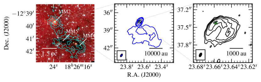
Figure 15: G018.82$-$00.28 - Mid-infrared (GLIMPSE $8.0,4.5,3.6\micron$ R, G, B image; left panel), sub-mm (ATLASGAL $870\micron$ cyan contours; left panel) and radio maps of G018.82$-$00.28 at C-band (blue contours; middle) and Q-band (black contours; right). Restoring beams were $0.558\arcsec\times 0.283\arcsec$ at $-33\degr$ and $0.072\arcsec\times 0.038\arcsec$ at $-26\degr$, while contour levels are $(-3,3,6,12,44,171)\times\sigma$ and $(-3,3,6,11,21,40)\times\sigma$ for C and Q-band respectively and ATLASGAL contours are set at $(-3,3,5,9,15)\times\sigma$ where $\sigma=82{\rm\thinspace mJy}/\mathrm{beam}$. Green crosses show 6.7${\rm\thinspace GHz}$ methanol maser positions from our data. In the infrared images, a white ellipse is used to denote the approximate PSF of the relevant instrument. All other symbols/values have the usual meaning. If RMS noises are displayed in a subplot, that is because in the location of the source the RMS noise diverges from that quoted in LABEL:tab:BeamsNoises.

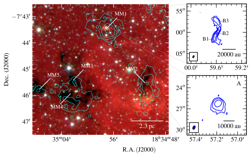
Figure 16: G024.08+00.04 - Mid-infrared (GLIMPSE $8.0,4.5,3.6\micron$ R, G, B image; left panel), sub-mm (ATLASGAL $870\micron$ cyan contours; left panel) and C-band (blue contours; right panels) images of G024.08+00.04. The C-band restoring beam was $0.551\arcsec\times 0.313\arcsec$ at $-25\degr$. The right panels show enlarged C-band maps of components A, B1, B2 and B3. Contour levels are $(-3,3,6,10,19)\times\sigma$ and ATLASGAL contours are set at $(-3,3,5,9,15)\times\sigma$ where $\sigma=75{\rm\thinspace mJy}/\mathrm{beam}$.

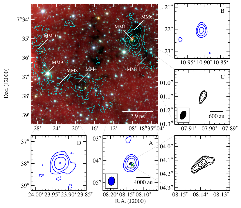
Figure 17: G024.33$+$00.11 - Mid-infrared (GLIMPSE $8.0,4.5,3.6\micron$ R, G, B image; top left panel), sub-mm (ATLASGAL $870\micron$ cyan contours; left panel) and radio contour maps of the IRDC, G024.33$+$00.11, at C-band (top and right panels; blue contours) and Q-band (middle and right panels; black contours). Restoring beams were $0.386\arcsec\times 0.297\arcsec$ at $-7\degr$ and $0.064\arcsec\times 0.038\arcsec$ at $-26\degr$ while contour levels are $(-3,3,7,16,36)\times\sigma$ and $(-3,3,4,6,9,13)\times\sigma$ for C and Q-band respectively and ATLASGAL contours are set at $(-3,3,7,15,32,70)\times\sigma$ where $\sigma=80{\rm\thinspace mJy}/\mathrm{beam}$. An exception to the contour levels is for component D which was much brighter than the other C-band sources and so we set its contour levels to $-4,4,12,37,111)\times\sigma$. All other values have the usual meaning.

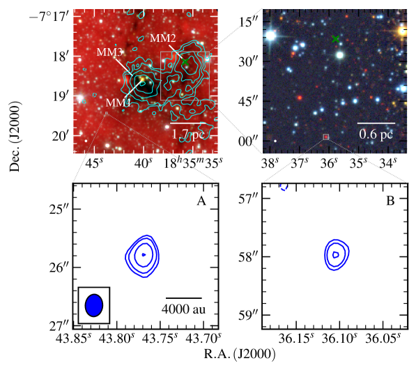
Figure 18: G024.60+00.08 - Mid-infrared (GLIMPSE $8.0,4.5,3.6\micron$ R, G, B image; top left panel), near-infrared (top right panel; UKIDSS, $\mathrm{K,H,J}$ bands in R, G, B colour-scale), sub-mm (ATLASGAL $870\micron$ cyan contours; top left panel) and C-band (blue contours; bottom panels) images of the IRDC, G024.60+00.08. The C-band restoring beam was $0.382\arcsec\times 0.297\arcsec$ at $-4\degr$. C-band contour levels are $(-3,3,5,10,18)\times\sigma$ and ATLASGAL contours are set at $(-3,3,5,8,14,24)\times\sigma$ where $\sigma=69{\rm\thinspace mJy}/\mathrm{beam}$. All other values have their usual meaning. Green crosses show 6.7${\rm\thinspace GHz}$ methanol maser positions from our data.

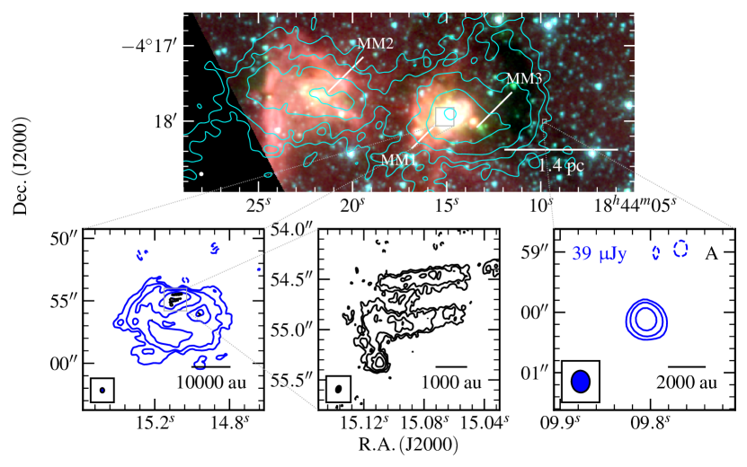
Figure 19: G028.28$-$00.34 - Mid-infrared (GLIMPSE $8.0,4.5,3.6\micron$ R, G, B image; top panel), sub-mm (ATLASGAL $870\micron$ cyan contours; top panel) and radio maps of G028.28$-$00.34 at C-band (blue contours; middle) and Q-band (black contours; bottom). Restoring beams were $0.364\arcsec\times 0.303\arcsec$ at $3\degr$ and $0.069\arcsec\times 0.047\arcsec$ at $-20\degr$, while contour levels are $(-3,3,10,33,108)\times\sigma$ and $(-3,3,5,9,17)\times\sigma$ for C and Q-band respectively. ATLASGAL contours are set at $(-3,3,6,11,20,39)\times\sigma$ where $\sigma=68{\rm\thinspace mJy}/\mathrm{beam}$. All other symbols/values have the usual meaning.

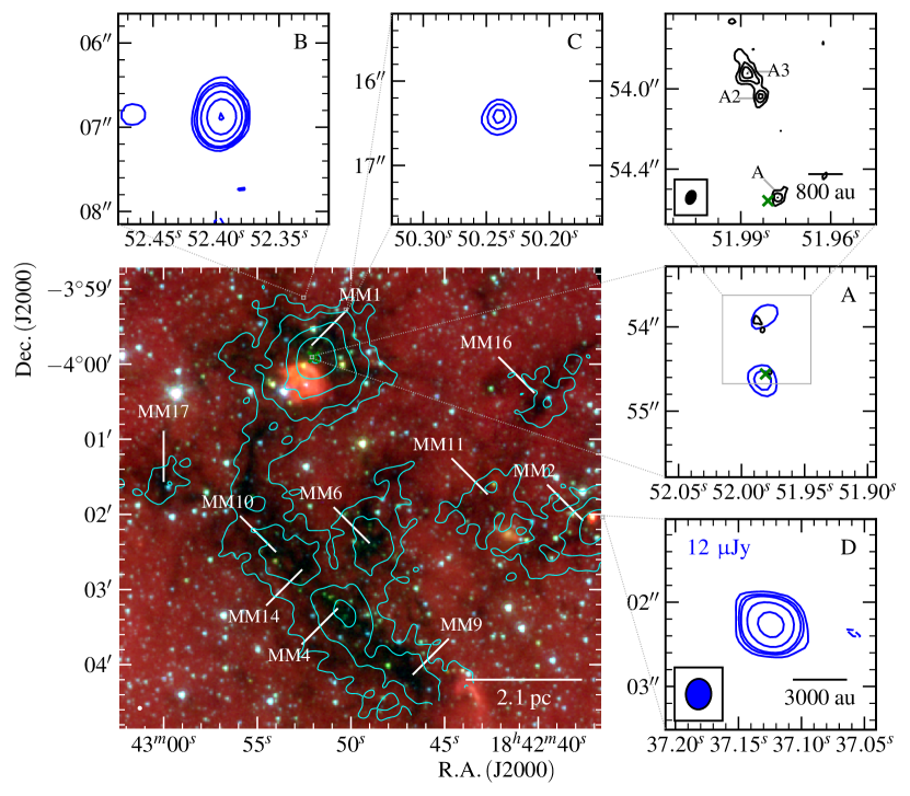
Figure 20: G028.37$+$00.07 - Mid-infrared (GLIMPSE $8.0,4.5,3.6\micron$ R, G, B image; left panel), sub-mm (ATLASGAL $870\micron$ cyan contours; left panel) and radio maps of G028.37$+$00.07 at C-band (blue contours; middle panels) and Q-band (black contours; right panel). Restoring beams were $0.364\arcsec\times 0.301\arcsec$ at $-3\degr$ and $0.068\arcsec\times 0.046\arcsec$ at $-21\degr$, while contour levels are $(-3,3,5,7,15,34,77)\times\sigma$ and $(-3,3,5,7,9)\times\sigma$ for C and Q-band respectively, while ATLASGAL contours are set at $(-3,3,6,13,28,59)\times\sigma$ where $\sigma=87{\rm\thinspace mJy}/\mathrm{beam}$. All other symbols/values have the usual meaning. Green crosses show 6.7${\rm\thinspace GHz}$ methanol maser positions from our data.

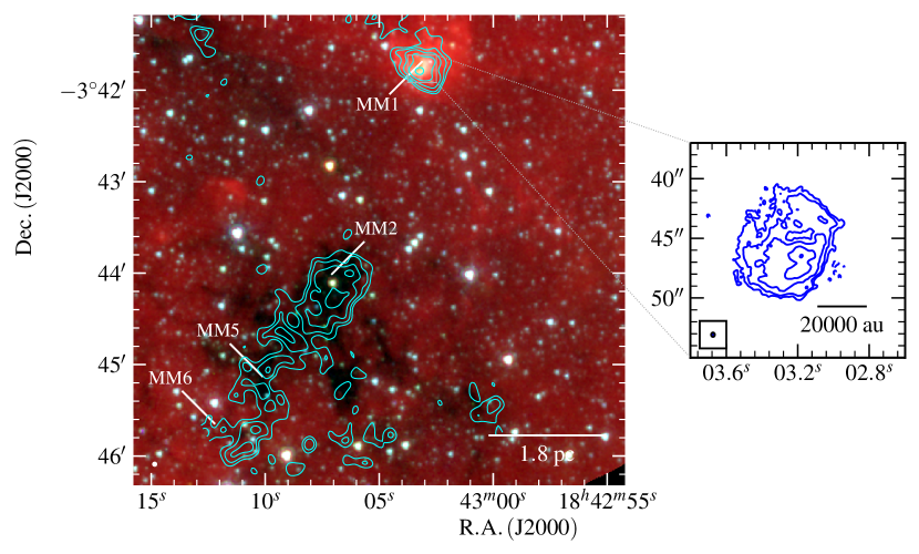
Figure 21: G028.67+00.13 - Mid-infrared (GLIMPSE $8.0,4.5,3.6\micron$ R, G, B image; left panel), sub-mm (ATLASGAL $870\micron$ cyan contours; left panel) and C-band radio map of G028.67+00.13 (right panel). The restoring beams used was $0.358\arcsec\times 0.303\arcsec$ at $1\degr$, while contour levels are set to $(-4,4,9,20,43,96)\times\sigma$. All other symbols/values have the usual meaning.

Figure 22: G033.69$-$00.01 - Mid-infrared (GLIMPSE $8.0,4.5,3.6\micron$ R, G, B image; left panel), sub-mm (ATLASGAL $870\micron$ cyan contours; left panel) and C-band radio map of G033.69$-$00.01 MM2 (right panel). The restoring beams used was $0.445\arcsec\times 0.364\arcsec$ at $-53\degr$, while contour levels are set to $(-4,4,7,13,22)\times\sigma$, while ATLASGAL contours are set at $(-3,3,5,9,15,25)\times\sigma$ where $\sigma=85{\rm\thinspace mJy}/\mathrm{beam}$. All other symbols/values have the usual meaning.

B.2 MYSO Sample

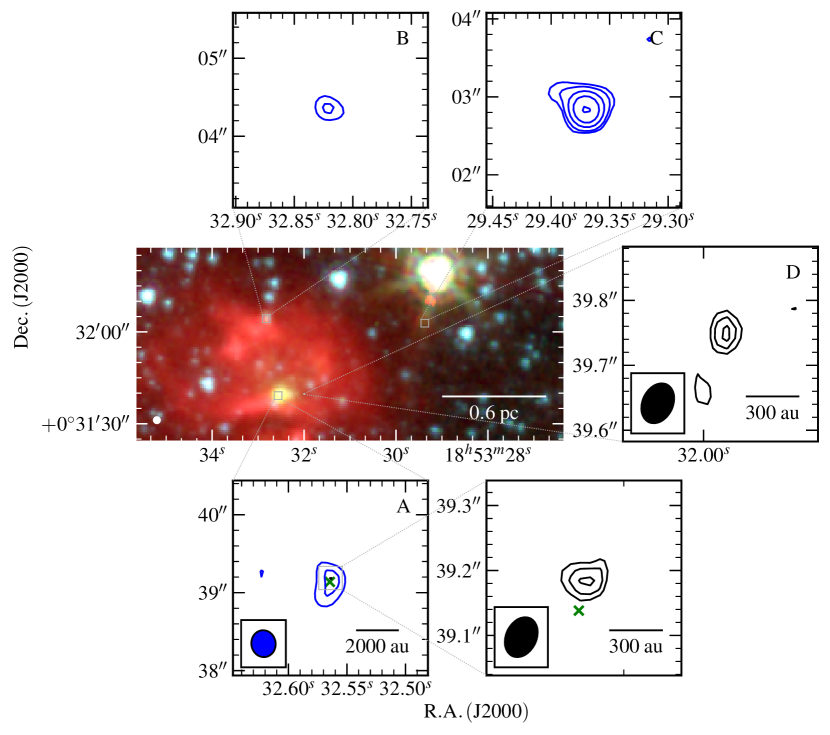
Figure 23: G033.6437$-$00.2277 - Mid-infrared (GLIMPSE $8.0,4.5,3.6\micron$ R, G, B image; left panel) and radio maps of G033.6437$-$00.2277 at C-band (blue contours; top and bottom left panels) and Q-band (black contours; bottom right and right panels). Restoring beams were $0.346\arcsec\times 0.311\arcsec$ at $9\degr$ and $0.064\arcsec\times 0.047\arcsec$ at $-26\degr$, while contour levels are $(-3,3,5,10,18,33)\times\sigma$ and $(-3,3,4,5)\times\sigma$ for C and Q-band respectively. All other symbols/values have the usual meaning. Green crosses show 6.7${\rm\thinspace GHz}$ methanol maser positions from our data.

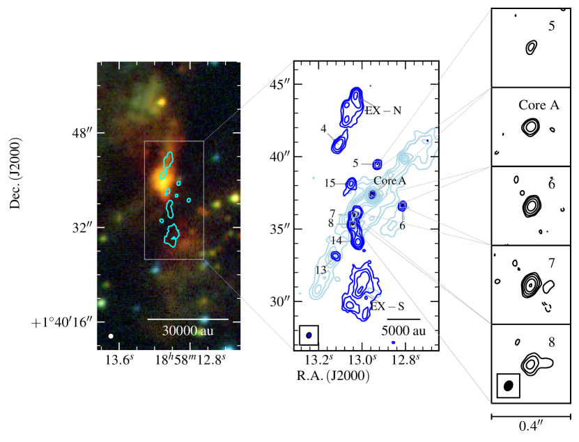
Figure 24: G035.1979$-$00.7427 - Mid-infrared (GLIMPSE $8.0,4.5,3.6\micron$ R, G, B image; left panel), ALMA $343{\rm\thinspace GHz}$ (Sánchez-Monge et al., 2014, light blue contours; middle panel), C-band (dark blue contours; middle panel) and Q-band (black contours; middle/right panels) images of G035.1979$-$00.7427 (or IRAS 18556+0136). Restoring beams were $0.367\arcsec\times 0.293\arcsec$ at $-21\degr$ and $0.051\arcsec\times 0.039\arcsec$ at $-29\degr$ for the C and Q-band data respectively. The right panels show enlarged maps of components 5, 6, 7, 8 and Core A at Q-band. Contour levels are $(-4,4,11,29,78)\times\sigma$ and $(-3,3,6,14,29,63)\times\sigma$ for C and Q-band respectively where $\sigma=35.1\,{\rm\thinspace\upmu Jy}\,{\rm beam}^{-1}$ for the Q-band image. All other values have the usual meaning.

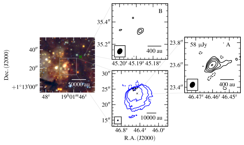
Figure 25: G035.1992$-$01.7424 - Near-infrared (R, G, B colour-scale, top left panel; UKIDSS, $\mathrm{K,H,J}$ bands), C-band (blue contours; bottom panel) and Q-band (black contours; top and right panels) images of W48 (G035.1992$-$01.7424). The C-band restoring beam was $0.364\arcsec\times 0.289\arcsec$ at $-21\degr$ and $0.051\arcsec\times 0.039\arcsec$ at $-31\degr$, while contour levels are $(-3,3,11,40,147)\times\sigma$ and $(-3,3,6,11,20,38)\times\sigma$ for the C and Q-band data respectively. All other values have their usual meaning.

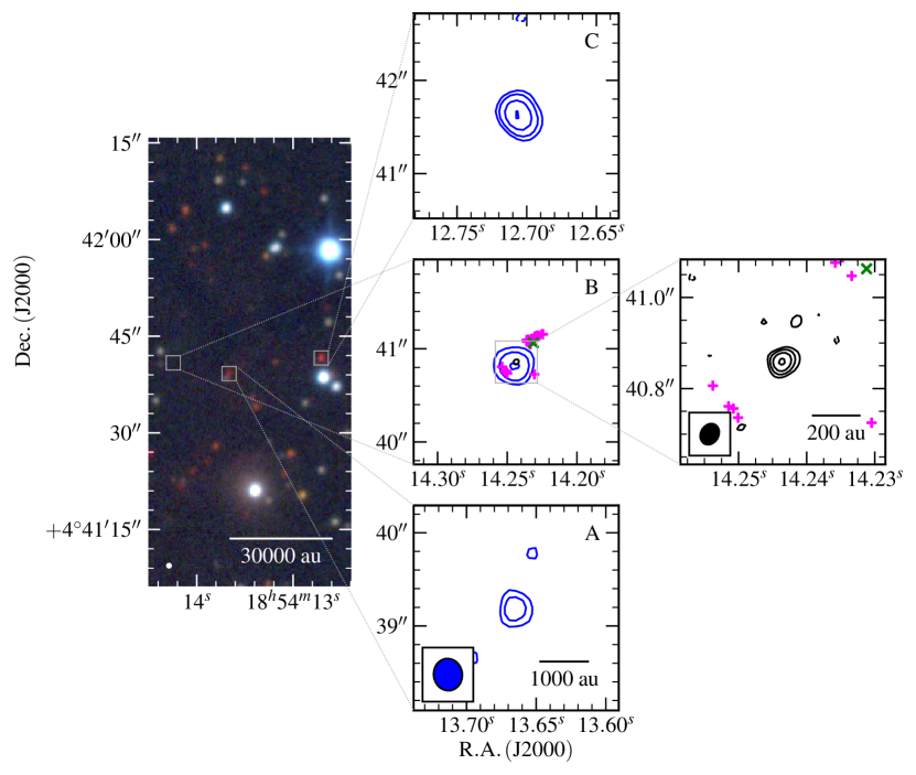
Figure 26: G037.4266+01.5183 - Near-infrared (R, G, B colour-scale, left panel; 2MASS, $\mathrm{K,H,J}$ bands) and radio contour maps of G037.4266+01.5183 (IRAS 18517+0437) at C-band (bottom, blue contours) and Q-band (bottom, black contours). Restoring beams were $0.344\arcsec\times 0.307\arcsec$ at $8\degr$ and $0.048\arcsec\times 0.039\arcsec$ at $-31\degr$ for the C and Q-band data respectively. The bottom panels show enlarged maps of components A, B and C at both bands. Contour levels are $(-3,3,5,9,15)\times\sigma$ and $(-3,3,5,8,13)\times\sigma$ for C and Q-band respectively. All other values have the usual meaning. Pink ’+’ markers represent the methanol masers detected by Surcis et al. (2015). Green crosses show 6.7${\rm\thinspace GHz}$ methanol maser positions from our data.

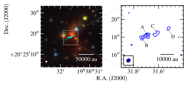
Figure 27: G056.3694$-$00.6333 - Near-infrared (left panel; UKIDSS, $\mathrm{K,H,J}$ bands in R, G, B colour-scale) and C-band radio map (robustness of 2) of G056.3694$-$00.6333 (right panel). The restoring beams used was $0.445\arcsec\times 0.364\arcsec$ at $-53\degr$, while contour levels are set to $(-3,3,5,7)\times\sigma$. All other symbols/values have the usual meaning. To highlight the slight offset between the reddened UKIDSS source and radio lobes, the radio $3\sigma$ contour is overlayed upon the NIR image (cyan).

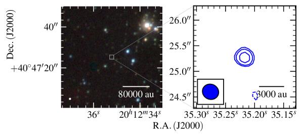
Figure 28: G077.5671+03.6911 - Near-infrared (left panel; UKIDSS, $\mathrm{K,H,J}$ bands in R, G, B colour-scale) and C-band radio map of G077.5671+03.6911 (right panel). The restoring beams used was $0.323\arcsec\times 0.295\arcsec$ at $66\degr$. Contour levels are $(-3,3,5,7)\times\sigma$. All other symbols/values have the usual meaning.

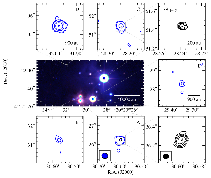
Figure 29: G078.8699+02.7602 - Near-infrared (middle row, left panel; UKIDSS, $\mathrm{K,H,J}$ R, G, B colour-scale) and radio maps of G078.8699+02.7602 at C-band (blue contours; middle row and top right panels) and Q-band (black contours; bottom panels). Restoring beams were $0.319\arcsec\times 0.295\arcsec$ at $61\degr$ and $0.062\arcsec\times 0.050\arcsec$ at $-85\degr$ for the C and Q-band data respectively. Contour levels are $(-3,3,6,16,35,80)\times\sigma$ for C-band images, $(-3,3,5,10,20,37)\times\sigma$ for the Q-band image of A and $(-3,3,5,8,12,19)\times\sigma$ for the Q-band image of C (due to varying noise across the primary beam). All other symbols/values have the usual meaning.

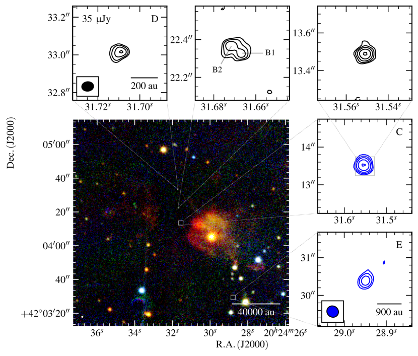
Figure 30: G079.8855+02.5517 - Near-infrared (bottom left panel; UKIDSS, $\mathrm{K,H,J}$ bands in R, G, B colour-scale) and radio maps of G079.8855+02.5517 at C-band (blue contours; top left, top middle, bottom left, bottom middle and middle right panels) and Q-band (black contours; top right/ bottom left panels). Restoring beams were $0.316\arcsec\times 0.293\arcsec$ at $54\degr$ and $0.062\arcsec\times 0.050\arcsec$ at $-84\degr$ for the C and Q-band data respectively. Contour levels are $(-3,3,6,11,22)\times\sigma$ for C-band and Q-band images of lobes A, B and C1/C2, whilst being $(-3,3,4,7,10)\times\sigma$ for the Q-band image of D (due to varying noise across the primary beam). All other symbols/values have the usual meaning.

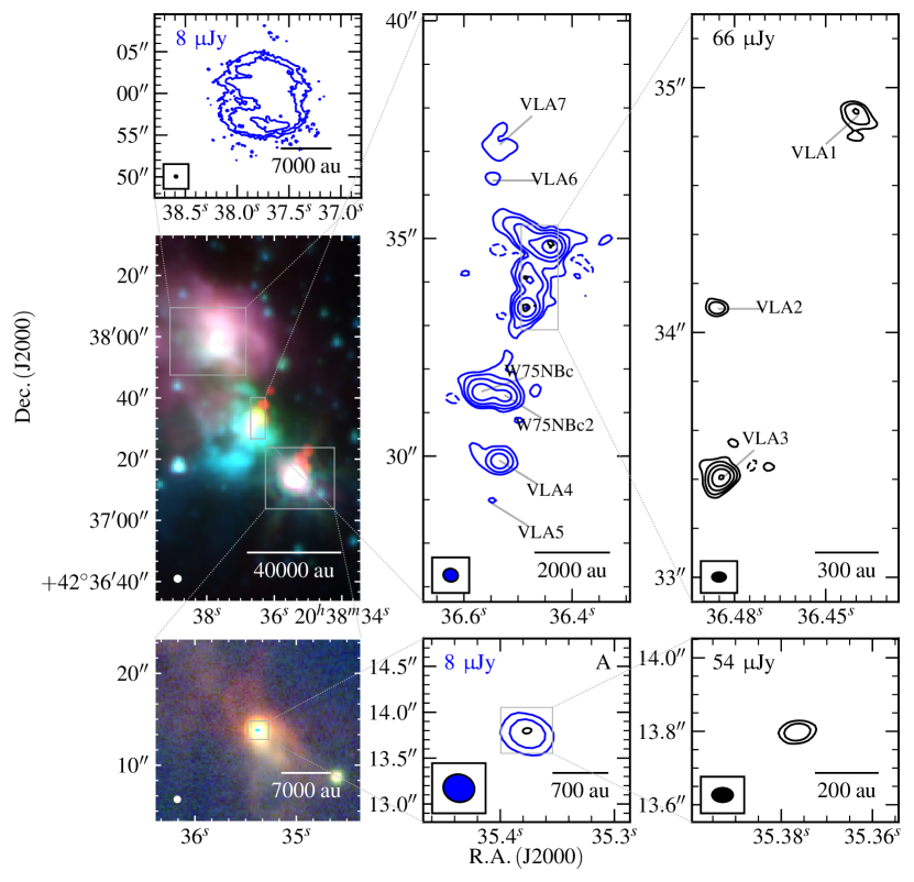
Figure 31: G081.8652+00.7800 - Mid-infrared (middle, left panel; GLIMPSE, $8.0,4.5,3.6\micron$ R, G, B colour-scale), near-infrared (bottom left panel; UKIDSS, $\mathrm{K,H,J}$ bands in R, G, B colour-scale) and radio maps of G081.8652+00.7800 at C-band (blue contours; middle, central and bottom-middle) and Q-band (black contours; right and bottom right). Restoring beams were $0.313\arcsec\times 0.293\arcsec$ at $43\degr$ and $0.051\arcsec\times 0.039\arcsec$ at $89\degr$, while contour levels are set at $(-4,4,9,21,49,112)$ and $(-4,4,10,25,61,153)\times\sigma$ for the C and Q-band data respectively. Varying noise levels are the result of dynamic range limitations leading to non-Gaussian noise as well as standard primary beam effects.

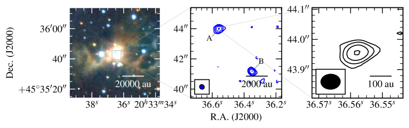
Figure 32: G083.7071+03.2817 - Near-infrared (left panel; UKIDSS, $\mathrm{K,H,J}$ bands in R, G, B colour-scale) and radio maps of G083.7071+03.2817 at C-band (blue contours; middle) and Q-band (black contours; bottom). Restoring beams were $0.319\arcsec\times 0.290\arcsec$ at $46\degr$ and $0.064\arcsec\times 0.050\arcsec$ at $-88\degr$ for the C and Q-band data respectively. Contour levels are $(-3,3,6,13,27)\times\sigma$ and $(-3,3,5,10,18)\times\sigma$ for C and Q-band respectively. All other symbols/values have the usual meaning.

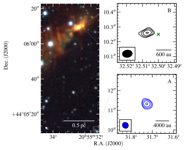
Figure 33: G084.9505$-$00.6910 - Near-infrared (left panel; UKIDSS, $\mathrm{K,H,J}$ bands in R, G, B colour-scale) and radio maps of the G084.9505$-$00.6910 field at C-band (blue contours; bottom right) and Q-band (black contours; top right). Restoring beams were $0.316\arcsec\times 0.292\arcsec$ at $45\degr$ and $0.067\arcsec\times 0.050\arcsec$ at $-83\degr$ for the C and Q-band (robustness of 2) data respectively. Contour levels are $(-3,3,5,9,16)\times\sigma$ and $(-3,3,4,6,8)\times\sigma$ for C and Q-band respectively. All other symbols/values have the usual meaning. Green crosses show 6.7${\rm\thinspace GHz}$ methanol maser positions from our data.

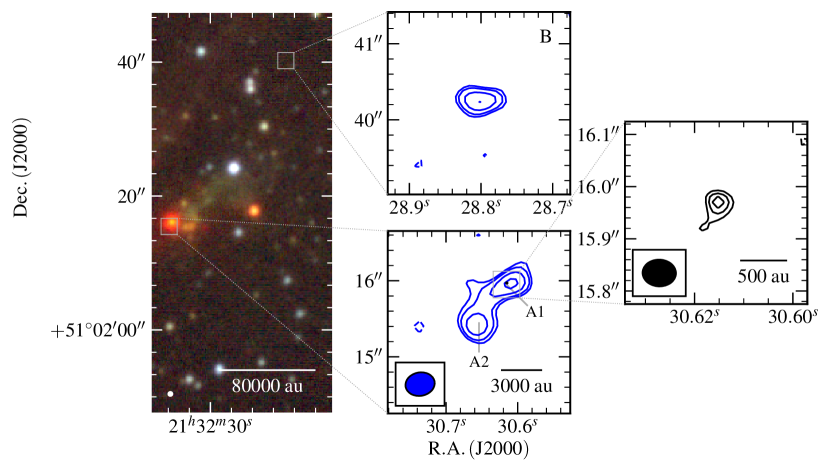
Figure 34: G094.2615$-$00.4116 - Near-infrared (left panel; UKIDSS, $\mathrm{K,H,J}$ bands in R, G, B colour-scale) and radio maps of the G094.2615$-$00.4116 field at C-band (blue contours; middle) and Q-band (black contours; right). Restoring beams were $0.387\arcsec\times 0.308\arcsec$ at $-80\degr$ and $0.064\arcsec\times 0.051\arcsec$ at $88\degr$ for the C and Q-band data respectively. Contour levels are $(-3,3,4,6,9)\times\sigma$ and $(-3,3,4,5)\times\sigma$ for C and Q-band (robustness of 2) respectively. All other symbols/values have the usual meaning.

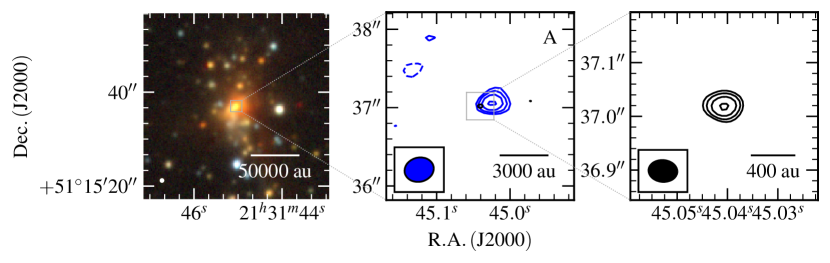
Figure 35: G094.3228$-$00.1671 - Near-infrared (left panel; UKIDSS, $\mathrm{K,H,J}$ bands in R, G, B colour-scale) and radio maps of the G094.3228$-$00.1671 field at C-band (blue contours; middle) and Q-band (black contours; right). Restoring beams were $0.377\arcsec\times 0.309\arcsec$ at $-77\degr$ and $0.054\arcsec\times 0.041\arcsec$ at $-85\degr$ for the C and Q-band data respectively. Contour levels are $(-3,3,4,6,8)\times\sigma$ and $(-3,3,4,7,10)\times\sigma$ for C and Q-band respectively. All other symbols/values have the usual meaning.

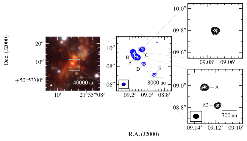
Figure 36: G094.4637$-$00.8043 - Near-infrared (left panel; UKIDSS, $\mathrm{K,H,J}$ bands in R, G, B colour-scale) and radio maps of the G094.4637$-$00.8043 field at C-band (blue contours; middle) and Q-band (black contours; right). Restoring beams were $0.392\arcsec\times 0.312\arcsec$ at $-82\degr$ and $0.053\arcsec\times 0.041\arcsec$ at $87\degr$ for the C and Q-band data respectively. Contour levels are $(-4,4,8,15,29)\times\sigma$ and $(-4,4,6,8,11,15)\times\sigma$ for C and Q-band respectively. All other symbols/values have the usual meaning.

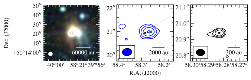
Figure 37: G094.6028$-$01.7966 - Near-infrared (left panel; 2MASS, $\mathrm{K,H,J}$ bands in R, G, B colour-scale) and radio maps of G094.6028$-$01.7966 at C-band (blue contours; middle) and Q-band (black contours; bottom). Restoring beams were $0.399\arcsec\times 0.311\arcsec$ at $-84\degr$ and $0.054\arcsec\times 0.041\arcsec$ at $88\degr$ for the C and Q-band data respectively. Contour levels are $(-3,3,7,15,32)\times\sigma$ and $(-3,3,5,9,15)\times\sigma$ for C and Q-band respectively. All other symbols/values have the usual meaning. Green crosses show 6.7${\rm\thinspace GHz}$ methanol maser positions from our data.

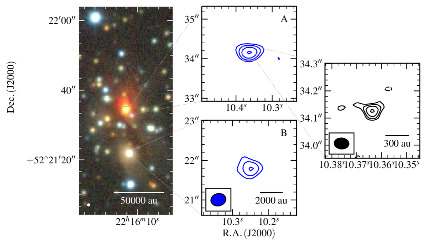
Figure 38: G100.3779$-$03.5784 - Near-infrared (left panel; UKIDSS, $\mathrm{K,H,J}$ bands in R, G, B colour-scale) and radio maps of the G100.3779$-$03.5784 field at C-band (blue contours; middle) and Q-band (black contours; right). Restoring beams were $0.381\arcsec\times 0.310\arcsec$ at $-76\degr$ and $0.054\arcsec\times 0.041\arcsec$ at $87\degr$ for the C and Q-band data respectively. Contour levels are $(-3,3,5,8,13)\times\sigma$ and $(-3,3,4,7,10)\times\sigma$ for C and Q-band (robustness of 2) respectively. All other symbols/values have the usual meaning.

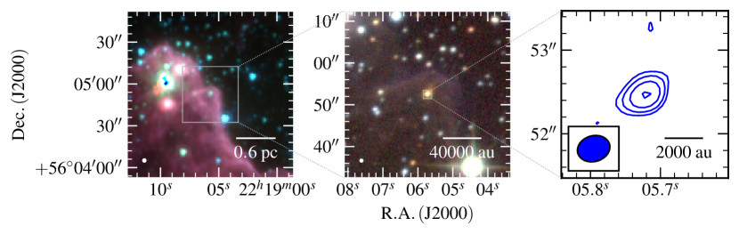
Figure 39: G102.8051$-$00.7184 - Mid-infrared (left panel; GLIMPSE, $8.0,4.5,3.6\micron$ R, G, B colour-scale), near-infrared (middle panel; UKIDSS, $\mathrm{K,H,J}$ bands in R, G, B colour-scale) and C-band radio map of G102.8051$-$00.7184 (right panel). The restoring beams used was $0.395\arcsec\times 0.309\arcsec$ at $-75\degr$. Contour levels are $(-3,3,5,9,14)\times\sigma$. All other symbols/values have the usual meaning.

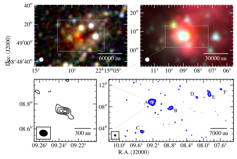
Figure 40: G103.8744+01.8558 - Mid-infrared (top right panel; GLIMPSE, $8.0,4.5,3.6\micron$ R, G, B colour-scale), near-infrared (top left panel; 2MASS, $\mathrm{K,H,J}$ R, G, B colour-scale) and radio maps of G103.8744+01.8558 at C-band (blue contours; bottom-right) and Q-band (black contours; bottom left). Restoring beams were $0.327\arcsec\times 0.302\arcsec$ at $54\degr$ and $0.065\arcsec\times 0.050\arcsec$ at $80\degr$, while contour levels are $(-3,3,5,9,24,70,199)\times\sigma$ and $(-3,3,4,5,6)\times\sigma$ for C and Q-band (robustness of 2) respectively. All other symbols have their usual meanings.

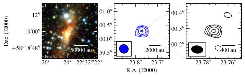
Figure 41: G105.5072+00.2294 - Near-infrared (R, G, B colour-scale, left panel; UKIDSS, $\mathrm{K,H,J}$ bands) and radio maps of the G105.5072+00.2294 field at C-band (blue contours; middle) and Q-band (black contours; right). Restoring beams were $0.330\arcsec\times 0.312\arcsec$ at $51\degr$ and $0.073\arcsec\times 0.048\arcsec$ at $83\degr$, while contour levels are $(-3,3,4,6,9)\times\sigma$ and $(-3,3,5,7,12)\times\sigma$ for C and Q-band (robustness of 2) respectively. All other symbols/values have the usual meaning.

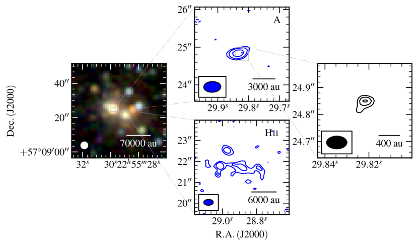
Figure 42: G107.6823$-$02.2423A - Near-infrared (R, G, B colour-scale, left panel; 2MASS, $\mathrm{K,H,J}$ bands) and radio contour maps of G107.6823$-$02.2423A at C-band (top and bottom panels; blue contours) and Q-band (right panel; black contours). Restoring beams were $0.564\arcsec\times 0.352\arcsec$ at $-88\degr$ and $0.075\arcsec\times 0.047\arcsec$ at $-90\degr$ while contour levels are $(-3,3,4,6,8)\times\sigma$ and $(-3,3,4,5)\times\sigma$ for C and Q-band respectively. A robustness of 2 was utilised for both sets of radio data. All other values have the usual meaning.

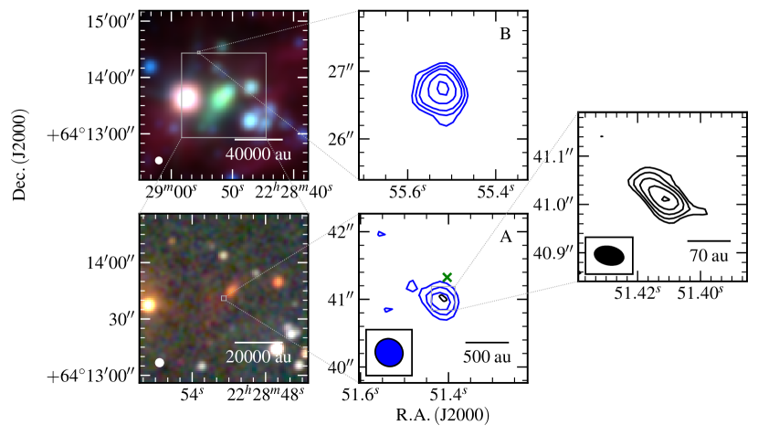
Figure 43: G108.1844+05.5187 - Mid-infrared (R, G, B colour-scale, top-left panel; WISE, $12.0,4.6,3.4\micron$), near-infrared (R, G, B colour-scale, bottom-left panel; 2MASS, $\mathrm{K,H,J}$ bands) and radio contour maps of G108.1844+05.5187 at C-band (top and bottom panels; blue contours) and Q-band (right panel; black contours). Restoring beams were $0.423\arcsec\times 0.398\arcsec$ at $45\degr$ and $0.061\arcsec\times 0.038\arcsec$ at $79\degr$ while contour levels are $(-3,3,4,5,7,9)\times\sigma$ and $(-3,3,5,7,11,16)\times\sigma$ for C and Q-band respectively. All other values have the usual meaning. Green crosses show 6.7${\rm\thinspace GHz}$ methanol maser positions from our data.

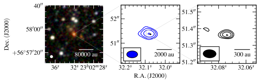
Figure 44: G108.4714$-$02.8176 - Near-infrared (left panel; 2MASS, $\mathrm{K,H,J}$ bands R, G, B colour-scale) and radio maps of the G108.4714$-$02.8176 field at C-band (blue contours; middle) and Q-band (black contours; right). Restoring beams were $0.445\arcsec\times 0.282\arcsec$ at $-90\degr$ and $0.063\arcsec\times 0.038\arcsec$ at $88\degr$ for the C and Q-band data respectively. Contour levels are $(-3,3,5,10,17)\times\sigma$ and $(-3,3,4,5,7)\times\sigma$ for C and Q-band respectively. All other symbols/values have the usual meaning.

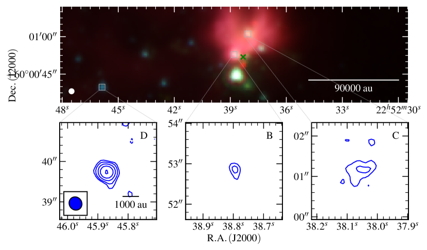
Figure 45: G108.5955+00.4935A - Mid-infrared (R, G, B colour-scale, top panel; GLIMPSE $8.0,4.5,3.6\micron$ bands) and C-band (blue contours; bottom panels) images of G108.5955+00.4935B and G108.5955+00.4935C. The C-band restoring beam was $0.337\arcsec\times 0.311\arcsec$ at $35\degr$. Contour levels are $(-3,3,5,9,15,26)\times\sigma$ and all other values have their usual meaning. It is important to note that the methanol maser indicated on the MIR plot (green cross) isn’t represented on radio images due to non-detection of continuum emission.

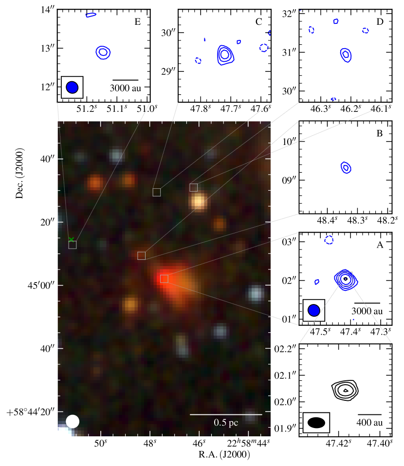
Figure 46: G108.7575$-$00.9863 - Mid-infrared (R, G, B colour-scale, left panel; 2MASS, $\mathrm{K,H,J}$ bands R, G, B colour-scale) and radio maps of G108.7575$-$00.9863 at C-band (blue contours; top and middle-right panels) and Q-band (black contours; bottom right). Restoring beams were $0.312\arcsec\times 0.295\arcsec$ at $44\degr$ and $0.063\arcsec\times 0.038\arcsec$ at $88\degr$, while contour levels were set at $(-3,3,5,8,12,19)$ and $(-3,3,5,9,15)\times\sigma$ for the C and Q-band (robustness of 2) data respectively. Varying noise levels are the result of missing spatial scale information leading to non-Gaussian noise and primary beam effects. Green crosses show 6.7${\rm\thinspace GHz}$ methanol maser positions from our data.

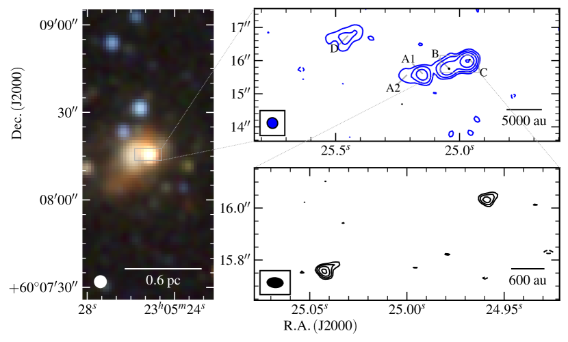
Figure 47: G110.0931$-$00.0641 - Near-infrared (R, G, B colour-scale, left panel; 2MASS, $\mathrm{K,H,J}$ bands ) and radio maps of the G110.0931$-$00.0641 field at C-band (blue contours; middle) and Q-band (black contours; right). Restoring beams were $0.326\arcsec\times 0.314\arcsec$ at $36\degr$ and $0.063\arcsec\times 0.038\arcsec$ at $86\degr$, while contour levels are $(-3,3,7,14,32,69)\times\sigma$ and $(-3,3,4,5,6)\times\sigma$ for C and Q-band respectively. All other symbols/values have the usual meaning.

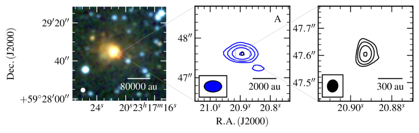
Figure 48: G111.2348$-$01.2385 - Near-infrared (left panel; 2MASS, $\mathrm{K,H,J}$ bands R, G, B colour-scale) and radio maps of the G111.2348$-$01.2385 field at C-band (blue contours; middle) and Q-band (black contours; right). Restoring beams were $0.443\arcsec\times 0.284\arcsec$ at $90\degr$ and $0.045\arcsec\times 0.039\arcsec$ at $-10\degr$ while contour levels are set at $(-3,3,6,12,24)\times\sigma$ and $(-3,3,6,12,25)\times\sigma$ for C and Q-band respectively. All other symbols/values have the usual meaning.

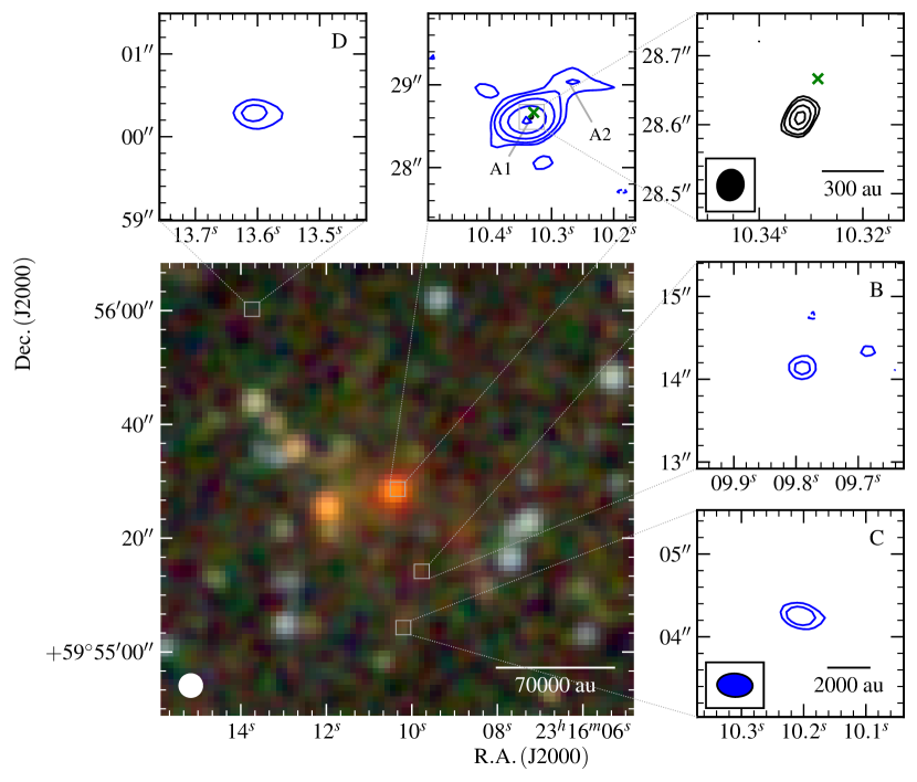
Figure 49: G111.2552$-$00.7702 - Near-infrared (bottom left panel; 2MASS, $\mathrm{K,H,J}$ R, G, B colour-scale) and radio maps of G111.2552$-$00.7702 at C-band (blue contours; top left/middle and right middle/bottom panels) and Q-band (black contours; top right panel). Restoring beams were $0.430\arcsec\times 0.283\arcsec$ at $87\degr$ and $0.045\arcsec\times 0.038\arcsec$ at $-11\degr$ while contour levels are set at $(-3,3,5,9,17,30)\times\sigma$ and $(-3,3,4,6,8)\times\sigma$ for the C-band and Q-band images respectively. All other symbols/values have the usual meaning. Green crosses show 6.7${\rm\thinspace GHz}$ methanol maser positions from our data.

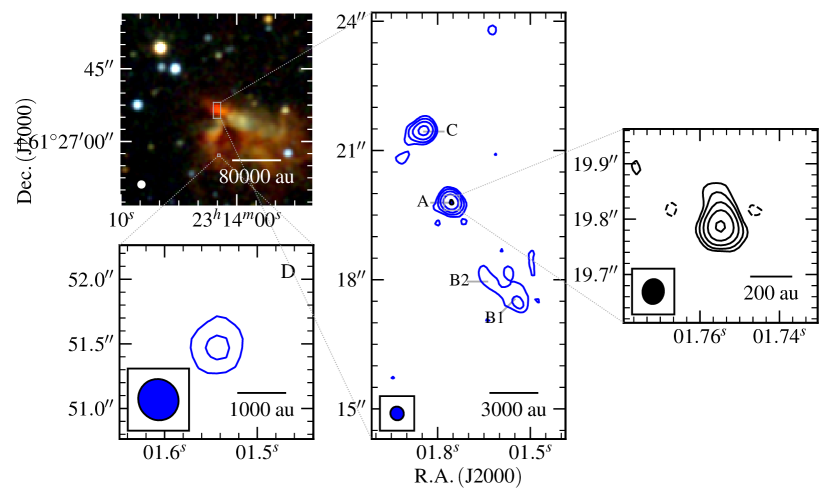
Figure 50: G111.5671+00.7517 - Near-infrared (R, G, B colour-scale, left panel; 2MASS, $\mathrm{K,H,J}$ bands) and radio contour maps of G111.5671+00.7517 at C-band (middle and bottom left panels; blue contours) and Q-band (right panel; black contours). Restoring beams were $0.324\arcsec\times 0.308\arcsec$ at $31\degr$ and $0.045\arcsec\times 0.038\arcsec$ at $-9\degr$ while contour levels are $(-3,3,6,12,24,48)\times\sigma$ and $(-3,3,6,12,23,46)\times\sigma$ for C and Q-band respectively. All other values have the usual meaning.

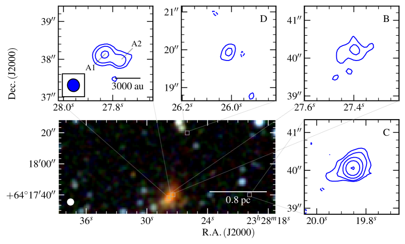
Figure 51: G114.0835+02.8568 - Near-infrared colour-scale (R, G, B colour-scale, left panel; 2MASS, $\mathrm{K,H,J}$ bands) and radio contour maps of G114.0835+02.8568 at C-band (blue contours). The restoring beam and contour levels used were $0.337\arcsec\times 0.317\arcsec$ at $13\degr$ and $(-3,3,6,14,30,64)\times\sigma$. All other values have the usual meaning.

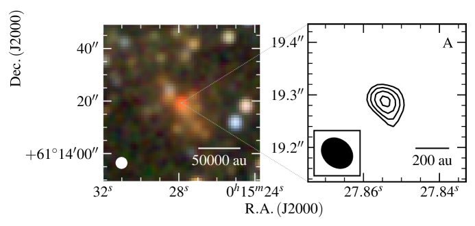
Figure 52: G118.6172$-$01.3312 - Near-infrared colour-scale (R, G, B colour-scale, left panel; 2MASS, $\mathrm{K,H,J}$ bands) and radio contour map of G118.6172$-$01.3312 at Q-band (right panel). The restoring beam and contour levels used were $0.064\arcsec\times 0.051\arcsec$ at $48\degr$ and $(-3,3,4,5,6)\times\sigma$ respectively. All other values have the usual meaning.

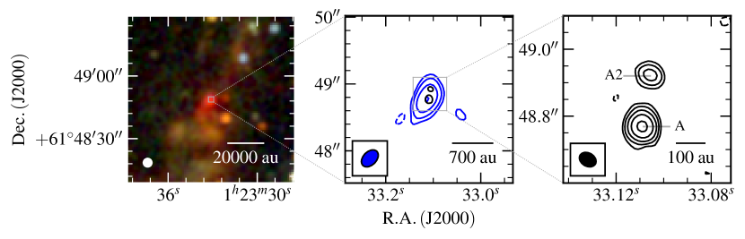
Figure 53: G126.7144$-$00.8220 - Near-infrared (left panel; 2MASS, $\mathrm{K,H,J}$ bands R, G, B colour-scale) and radio maps of the G126.7144$-$00.8220 field at C-band (blue contours; middle) and Q-band (black contours; right). Restoring beams were $0.295\arcsec\times 0.200\arcsec$ at $-44\degr$ and $0.053\arcsec\times 0.040\arcsec$ at $60\degr$, while contour levels are $(-3,3,7,18,43)\times\sigma$ and $(-3,3,7,16,37,86)\times\sigma$ for C (robustness of -1) and Q-band respectively. All other symbols/values have the usual meaning.

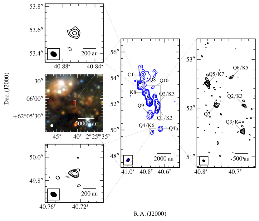
Figure 54: G133.7150+01.2155 - Near-infrared (R, G, B colour-scale, middle left panel; 2MASS, $\mathrm{K,H,J}$ bands) and radio contour maps of G133.7150+01.2155 at C-band (middle, blue contours) and Q-band (top left, bottom right and right panels; black contours). Restoring beams were $0.287\arcsec\times 0.197\arcsec$ at $-31\degr$ and $0.054\arcsec\times 0.038\arcsec$ at $59\degr$ with contour levels set to $(-4,4,9,19,42,93)\times\sigma$ and $(-3,3,6,12,24,48)\times\sigma$ for C (robust$=-1$) and Q-bands respectively. All other values have the usual meaning.

Figure 55: G133.7150+01.2155 (Other sources) - Near-infrared (R, G, B colour-scale, middle left panel; 2MASS, $\mathrm{K,H,J}$ bands) and radio contour maps of the other detected sources in the G133.7150+01.2155 field. Restoring beams and contour colours are the same as in Figure 54, with contour levels set to $(-3,3,5,8,14,22)\times\sigma$ and $(-3,3,5,12,24,47)\times\sigma$ for C (robust$=-1$) and Q-bands respectively.

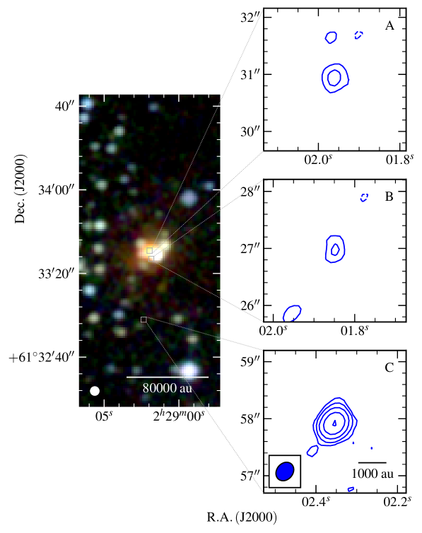
Figure 56: G134.2792+00.8561 - Near-infrared (R, G, B colour-scale, left panel; 2MASS, $\mathrm{K,H,J}$ bands) and radio contour maps of G134.2792+00.8561 at C-band (right panels, blue contours). The restoring beam used was $0.350\arcsec\times 0.284\arcsec$ at $-40\degr$, while contour levels are $(-3,3,7,17,41,97)\times\sigma$. All other values have the usual meaning.

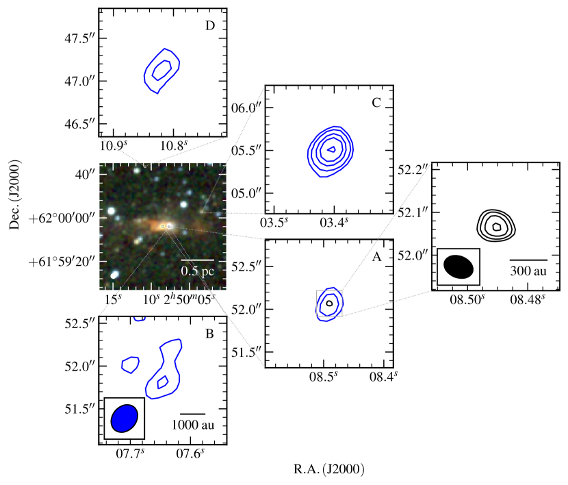
Figure 57: G136.3833+02.2666 - Near-infrared (R, G, B colour-scale, left panel; 2MASS, $\mathrm{K,H,J}$ bands) and radio contour maps of G136.3833+02.2666 at C-band (top left, bottom left and middle panels, blue contours) and Q-band (right panel, black contours). Restoring beams were $0.349\arcsec\times 0.279\arcsec$ at $-40\degr$ and $0.070\arcsec\times 0.050\arcsec$ at $69\degr$ utilising a robustness of 2 for the Q-band data. Contour levels are $(-3,3,5,9,13,20)\times\sigma$ and $(-3,3,4,6,9)\times\sigma$ for C and Q-band respectively. Varying noises across the C-band primary beam are represented. All other values have the usual meaning.

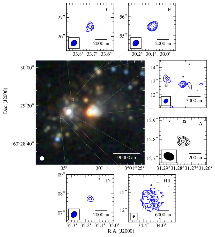
Figure 58: G138.2957+01.5552 - Near-infrared (R, G, B colour-scale, central panel; 2MASS, $\mathrm{K,H,J}$ bands) and radio contour maps of G138.2957+01.5552 at C-band (top, bottom and top-right panels, blue contours) and Q-band (bottom-right panel, black contours). Restoring beams were $0.342\arcsec\times 0.273\arcsec$ at $-42\degr$ and $0.056\arcsec\times 0.039\arcsec$ at $69\degr$. Contour levels are $(-3,3,5,8,13,22)\times\sigma$ and $(-3,3,5,7,10)\times\sigma$ for C and Q-band respectively. All other values have the usual meaning.

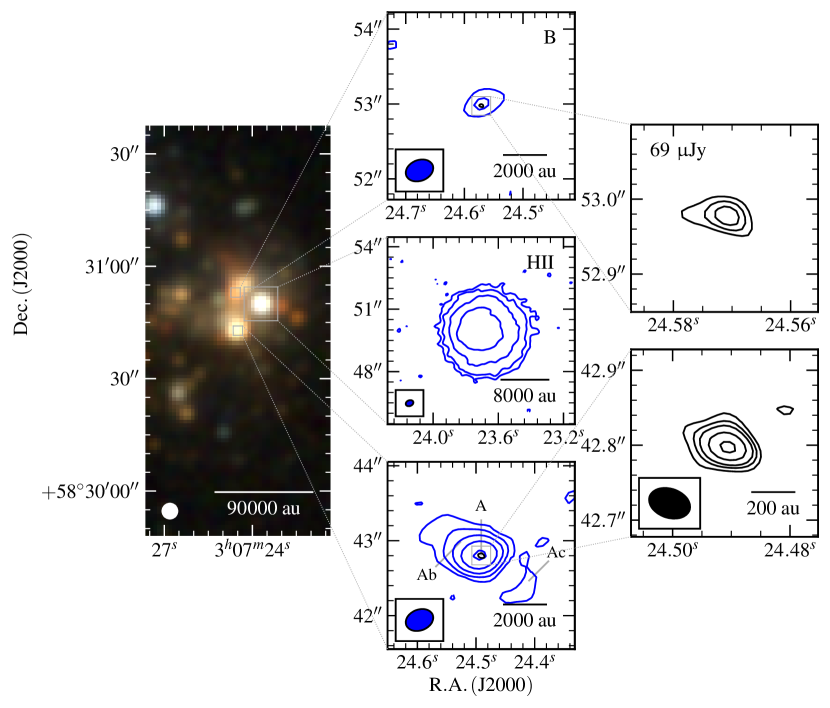
Figure 59: G139.9091+00.1969A - Near-infrared (R, G, B colour-scale, left panel; 2MASS, $\mathrm{K,H,J}$ bands) and radio contour maps of G139.9091+00.1969A at C-band (centre-column panels, blue contours) and Q-band (right panels, black contours). Restoring beams were $0.379\arcsec\times 0.278\arcsec$ at $-69\degr$ and $0.056\arcsec\times 0.039\arcsec$ at $71\degr$. Contour levels are $(-3,3,7,15,32,71)\times\sigma$ and $(-3,3,5,7,11,16)\times\sigma$ for C and Q-band respectively. All other values have the usual meaning.

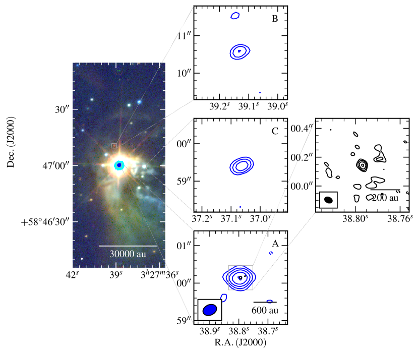
Figure 60: G141.9996+01.8202 - Near-infrared (R, G, B colour-scale, left panel; UKIDSS, $\mathrm{K,H,J}$ bands) and radio contour maps of G141.9996+01.8202 at C-band (centre-column panels, blue contours) and Q-band (right panel, black contours). Restoring beams were $0.379\arcsec\times 0.277\arcsec$ at $-66\degr$ and $0.055\arcsec\times 0.039\arcsec$ at $66\degr$. Contour levels are $(-3,3,6,11,20,37)\times\sigma$ and $(-3,3,5,7,12)\times\sigma$ for C and Q-band respectively. All other values have the usual meaning.

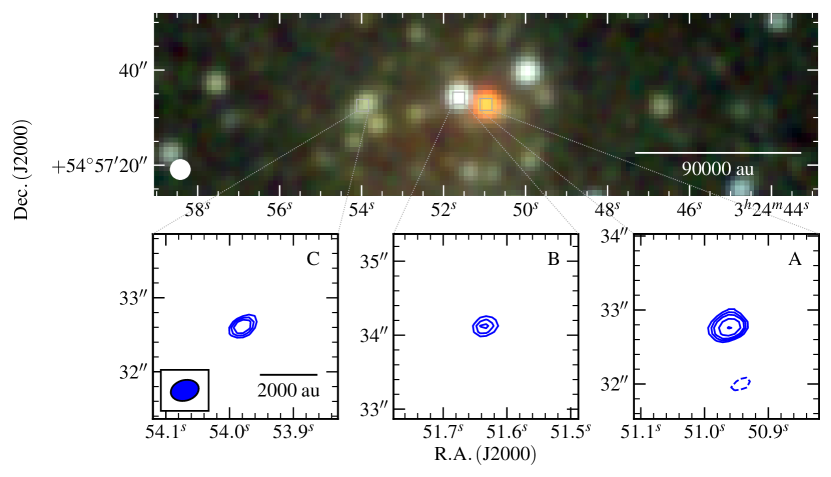
Figure 61: G143.8118$-$01.5699 - Near-infrared (R, G, B colour-scale, top panel; 2MASS, $\mathrm{K,H,J}$ bands) and C-band contour maps of G143.8118$-$01.5699 (bottom panels; blue contours). The restoring beams used was $0.384\arcsec\times 0.277\arcsec$ at $-75\degr$ and contour levels are $(-3,3,4,5,7,10)\times\sigma$. All other values have the usual meaning.

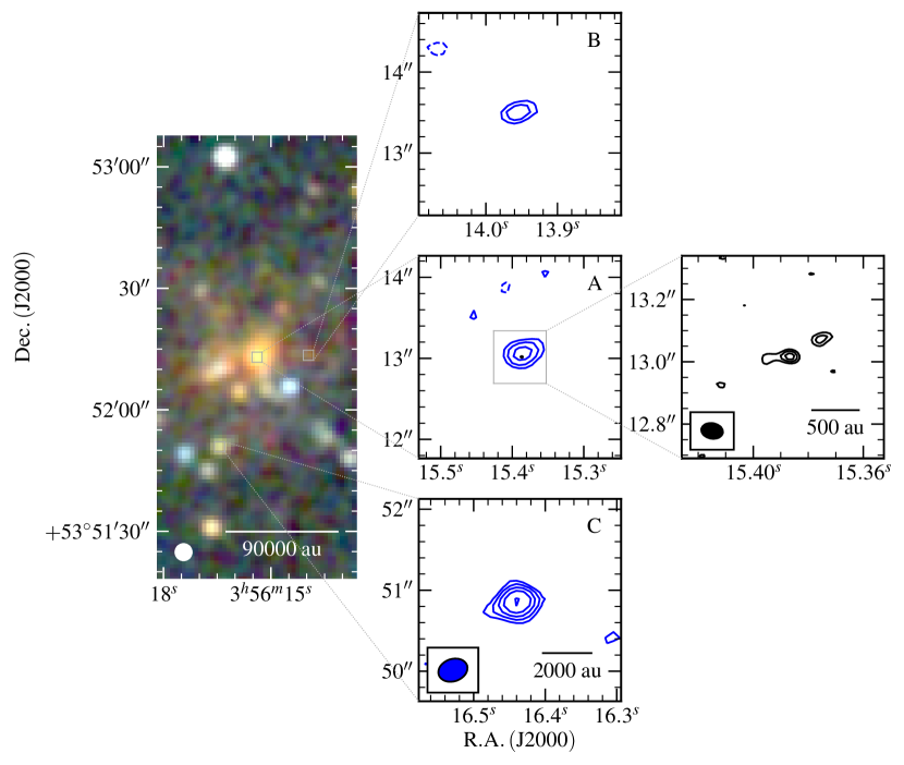
Figure 62: G148.1201+00.2928 - Near-infrared (R, G, B colour-scale, left panel; 2MASS, $\mathrm{K,H,J}$ bands) and radio contour maps of G148.1201+00.2928 at C-band (centre-column panels, blue contours) and Q-band (right panel, black contours). Restoring beams were $0.368\arcsec\times 0.275\arcsec$ at $-71\degr$ and $0.070\arcsec\times 0.050\arcsec$ at $80\degr$. Contour levels are $(-3,3,5,8,12,20)\times\sigma$ and $(-3,3,4,5)\times\sigma$ for C and Q-band (robustness of 2) respectively. All other values have the usual meaning.

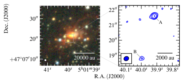
Figure 63: G160.1452+03.1559 - Near-infrared (R, G, B colour-scale, left panel; UKIDSS, $\mathrm{K,H,J}$ bands) and radio contour maps of G160.1452+03.1559 at C-band (right panel, blue contours). The restoring beam for the C-band data was $0.328\arcsec\times 0.280\arcsec$ at $-62\degr$, while contour levels are set at $(-3,3,5,8,13)\times\sigma$. All other values have the usual meaning.

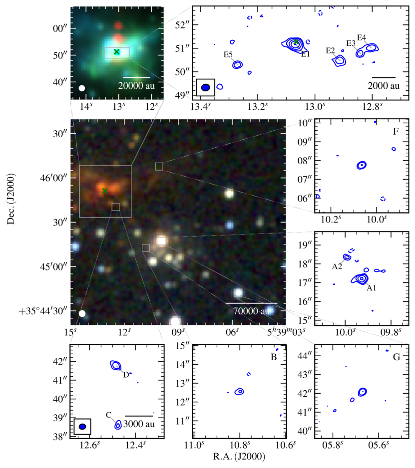
Figure 64: G173.4839+02.4317 - Near-infrared (R, G, B colour-scale, central, large panel; 2MASS, $\mathrm{K,H,J}$ bands), mid-infrared (R, G, B colour-scale, top left panel; GLIMPSE $8.0,4.5,3.6\micron$ bands) and radio contour maps of G173.4839+02.4317 at C-band (other panels, blue contours). The restoring beam for the C-band data was $0.347\arcsec\times 0.286\arcsec$ at $-84\degr$, while contour levels are set at $(-3,3,5,8,14,24)\times\sigma$. All other values have the usual meaning. Green crosses show 6.7${\rm\thinspace GHz}$ methanol maser positions from our data.

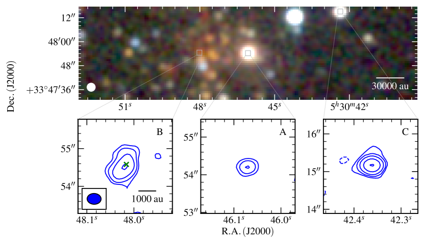
Figure 65: G174.1974$-$00.0763 - Near-infrared (R, G, B colour-scale, central, large panel; 2MASS, $\mathrm{K,H,J}$ bands) and radio contour maps of G174.1974$-$00.0763 at C-band (other panels, blue contours). The restoring beam for the C-band data was $0.369\arcsec\times 0.286\arcsec$ at $88\degr$, while contour levels are set at $(-3,3,7,17,46,114)\times\sigma$. All other values have the usual meaning. Green crosses show 6.7${\rm\thinspace GHz}$ methanol maser positions from our data.

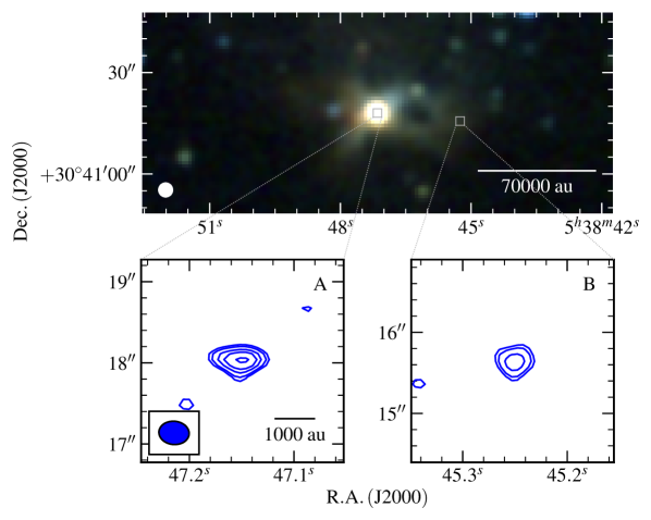
Figure 66: G177.7291$-$00.3358 - Near-infrared (R, G, B colour-scale, central, large panel; 2MASS, $\mathrm{K,H,J}$ bands) and C-band (blue contours; bottom panels) images of G177.7291$-$00.3358. The C-band restoring beam was $0.374\arcsec\times 0.288\arcsec$ at $84\degr$. Contour levels are $(-3,3,4,6,8,11)\times\sigma$ and all other values have their usual meaning.

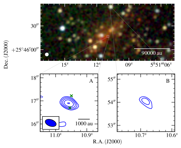
Figure 67: G183.3485$-$00.5751 - Near-infrared (R, G, B colour-scale, central, large panel; 2MASS, $\mathrm{K,H,J}$ bands) and C-band (blue contours; bottom panels) images of G183.3485$-$00.5751. The C-band restoring beam was $0.495\arcsec\times 0.285\arcsec$ at $70\degr$. Contour levels are $(-3,3,5,8,12,19)\times\sigma$ and all other values have their usual meaning. Green crosses show 6.7${\rm\thinspace GHz}$ methanol maser positions from our data.

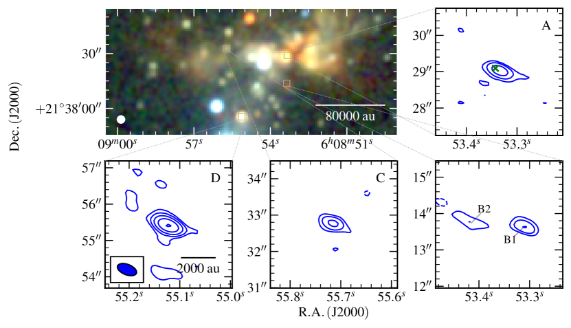
Figure 68: G188.9479+00.8871 - Near-infrared (R, G, B colour-scale, top left panel; 2MASS, $\mathrm{K,H,J}$ bands) and C-band (blue contours; bottom and top right panels) images of G188.9479+00.8871. The C-band restoring beam was $0.558\arcsec\times 0.290\arcsec$ at $69\degr$. Contour levels are $(-3,3,6,12,24,48)\times\sigma$ and all other values have their usual meaning. Green crosses show 6.7${\rm\thinspace GHz}$ methanol maser positions from our data.

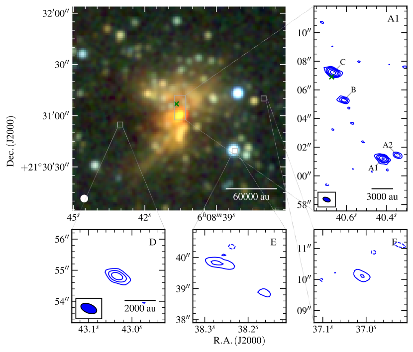
Figure 69: G189.0307+00.7821 - Near-infrared (R, G, B colour-scale, top left panel; 2MASS, $\mathrm{K,H,J}$ bands) and C-band (blue contours; bottom and top right panels) images of G189.0307+00.7821. The C-band restoring beam was $0.539\arcsec\times 0.291\arcsec$ at $68\degr$. Contour levels are $(-3,3,6,10,19,34)\times\sigma$ and all other values have their usual meaning. Green crosses show 6.7${\rm\thinspace GHz}$ methanol maser positions from our data.

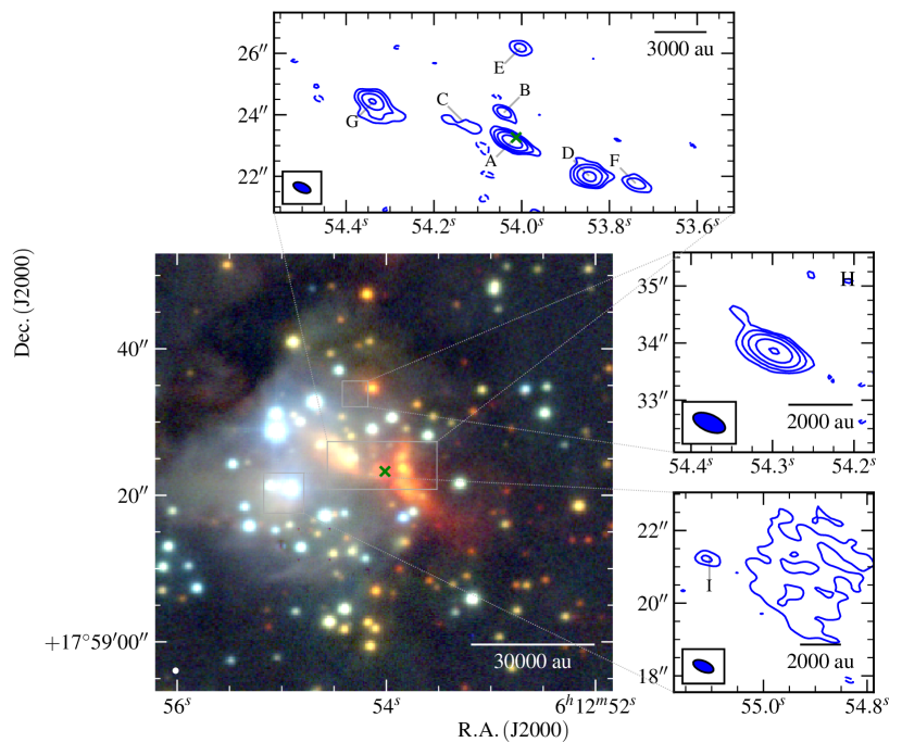
Figure 70: G192.6005$-$00.0479 - Near-infrared (R, G, B colour-scale, bottom left panel; UKIDSS, $\mathrm{K,H,J}$ bands) and C-band (blue contours; other panels) images of G192.6005$-$00.0479. The C-band restoring beam was $0.597\arcsec\times 0.292\arcsec$ at $67\degr$. Contour levels are $(-3,3,7,16,38,87)\times\sigma$ and all other values have their usual meaning.

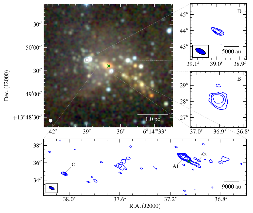
Figure 71: G196.4542$-$01.6777 - Near-infrared (R, G, B colour-scale, top left panel; UKIDSS, $\mathrm{K,H,J}$ bands) and C-band (blue contours; other panels) images of G196.4542$-$01.6777. The C-band restoring beam was $0.674\arcsec\times 0.293\arcsec$ at $63\degr$. Contour levels are $(-3,3,5,7,13,27,55)\times\sigma$ and all other values have their usual meaning. Green crosses show 6.7${\rm\thinspace GHz}$ methanol maser positions from our data.

Appendix C Calculation of mass loss rates

For calculating the mass loss rate of an ionised outflow, one of two approaches is used based upon the thermal emission’s spectral index. These approaches are summarised in Figure 72 and discussed below.

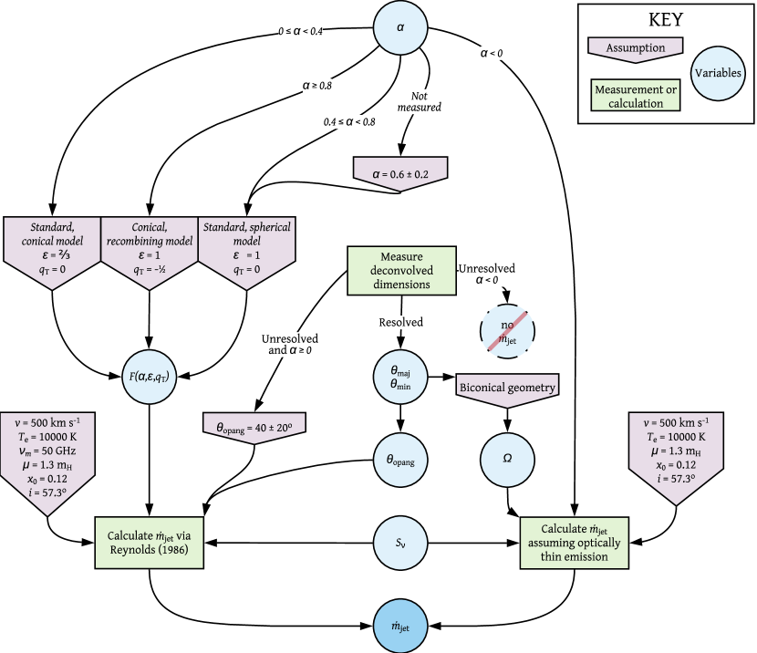
Figure 72: Paradigm used for calculating mass loss rate, $\dot{m}_{\rm jet}$, in ionised jets and disc-winds.

In cases where $\alpha\geq 0$, we use the analytical work of Reynolds (1986). Mass loss rates are calculated using Equation 11 for which one of three physical jet-models is selected to calculate a value for $F\left(\alpha,\epsilon,q_{\rm T}\right)$ (Equation 12) . Each model differs in its power-law describing jet-width and temperature as functions of distance along the jet’s axis, which are $w\left(r\right)\propto r^{\epsilon}$ and $T\left(r\right)\propto r^{q_{\rm T}}$, respectively. In cases where $0\leq\alpha<0.4$ we adopt the ‘standard, conical’ model representing jets whose material is still undergoing significant collimation, with $\epsilon=\nicefrac{{2}}{{3}}$ and $q_{\rm T}=0$. For $0.4\leq\alpha<0.8$ the ‘standard, spherical’ model is used with $\epsilon=1$ and $q_{\rm T}=0$, whereby jet material is ballistic with no significant collimation. Finally, for $\alpha\geq 0.8$ the ‘conical, recombining’ model is used with $\epsilon=1$ and $q_{\rm T}=-\nicefrac{{1}}{{2}}$ to approximate jets with some degree of recombination/cooling in their flow. Deconvolved dimensions (from CASA’s imfit task) are used to calculate opening angle whereby $\theta_{\rm 0}=\tan^{-1}\left(\nicefrac{{\theta_{\rm maj}}}{{\theta_{\rm min}}}\right)$. Assumed values for velocity, temperature, turnover frequency, mean atomic weight, ionisation fraction and inclination are $v=500\hbox{${\thinspace\rm{\rm\thinspace km}{\rm\thinspace s}^{-1}\,}$}$ (typical of MYSO jets), $T_{\rm e}=10000{\rm\thinspace K}$ (above which collisional cooling with metals is significant), $\nu_{\rm m}=50{\rm\thinspace GHz}$ (a lower limit from observational consensus), $\mu=1.3\,m_{\rm H}$ (typical solar abundances; Lodders, 2003), $x_{\rm 0}=12\%$ (from Fedriani et al., 2019) and $i=57\aas@@fstack{\circ}3$ (average inclination of a uniformly-distributed, random sample), respectively. In cases where no deconvolved dimensions could be measured, the weighted average opening angle of all jets from P16 and this work is used, $\theta_{0}=35\pm 16^{\circ}$.

$$\left[\frac{\dot{m}_{\rm jet}}{\rm M_{\odot}\,{\rm\thinspace yr}^{-1}}\right] =1.17\times 10^{12}\frac{v_{\rm jet}\,\mu\,S_{\nu}^{\nicefrac{{3}}{{4}}}\,D^{\nicefrac{{3}}{{2}}}\,\nu_{\rm m}^{\nicefrac{{3\alpha}}{{4}}-\nicefrac{{9}}{{20}}}\,\theta_{\mathrm{0}}^{\nicefrac{{3}}{{4}}}}{x_{\rm 0}\,\nu^{\nicefrac{{3\alpha}}{{4}}}\,T_{e}^{\nicefrac{{3}}{{40}}}\,\sin\left(i\right)^{\nicefrac{{1}}{{4}}}\,F\left(\alpha,\epsilon,q_{\rm T}\right)^{\nicefrac{{3}}{{4}}}}$$ (11)

$$F\left(\alpha,\epsilon,q_{\rm T}\right) =\frac{4.41}{q_{\tau}(\alpha-2)(\alpha+0.1)}$$ (12)

$$q_{\tau} =\frac{2.1\left(1+\epsilon+q_{T}\right)}{\alpha-2}$$

where all quantities are in SI units, unless explicitly stated.

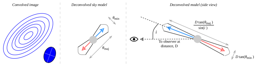
Figure 73: General schematic of an ionised jet, its dimensions and their relation to a clean radio image. Blue and red arrows indicate the jet moving towards and away from the observer, respectively.

For those jets with $\alpha<0$, we take a second approach. Since optically thin, radio emission in this case is a measure of the full, ionised content of the emitting plasma. We approximate the jet as having biconical geometry with a total length, $D\,\tan\left(\theta_{\rm maj}\right)\,\sin\left(i\right)^{-1}$ and width, $D\,\tan\left(\theta_{\rm min}\right)$ (see Figure 73). This leads to solid angle and volume as defined in Equations 13 and 14. Since we are in the regime whereby $h\nu\ll kT$ (assuming $T_{\rm e}=10000{\rm\thinspace K}$), the Rayleigh-Jeans approximation can be used in conjunction with $T_{\rm b}=T_{\rm e}\left(1-{\rm e}^{-\tau_{\rm\nu}}\right)$ to calculate the optical depth of the plasma (Equation 15). The amount of plasma along the line of sight, or emission measure, can be computed (in units of ${\rm\thinspace pc}\,{\rm\thinspace cm}^{-6}$) using Equation 16 (Mezger & Henderson, 1967) where the Gaunt factor is $\langle g_{\rm ff}\rangle=\ln(4.955\times 10^{7}\,\nu)+1.5\ln\left(T_{\rm e}\right)$. With a value for emission measure the average electron density, $n_{\rm e}$, within the biconical jet can be calculated since $EM=\int n_{\rm e}^{2}\,ds$. Constant density is assumed and the average jet thickness, $ds=D\,\tan\left(\theta_{\rm min}\right)\left[2\,\sin\left(i\right)\right]^{-1}$, is used. Mass loss rate is thereby computed using Equation 17 assuming a constant velocity over the timescale, $t=D\,\tan\left(\theta_{\rm maj}\right)\,\left(2\,\sin\left(i\right)v_{\rm jet}\right)^{-1}$. For the other parameters the same values are used as with the alternate method detailed above. In the cases where no deconvolved dimensions could be measured, no mass loss rate is derived.

$$\Omega =\frac{\theta_{\rm maj}\,\theta_{\rm min}}{2}$$ (13)

$$V =\frac{\pi\,D^{3}\,\tan\left(\theta_{\rm maj}\right)\,\tan^{2}\left(\theta_{\rm min}\right)}{12\sin\left(i\right)}$$ (14)

$$\tau_{\rm\nu} =-\ln\left(1-\frac{S_{\rm\nu}\,c^{2}}{2\,k_{\rm B}\,\nu^{2}\,\Omega\,T_{\rm e}}\right)$$ (15)

$$\left[\frac{EM}{\rm{\rm\thinspace pc}{\rm\thinspace cm}^{-6}}\right] =3.318\times 10^{-17}\,\tau_{\nu}\,T^{\nicefrac{{3}}{{2}}}_{\rm e}\,\nu^{2}\langle g_{\rm ff}\rangle^{-1}$$ (16)

$$\left[\frac{\dot{m}_{\rm jet}}{\rm M_{\odot}\,{\rm\thinspace yr}^{-1}}\right] =3.171\times 10^{-23}\frac{V\,n_{\rm e}\,\mu\,\sin\left(i\right)v_{\rm jet}}{D\,\tan\left(\theta_{\rm maj}\right)\,x_{0}}$$ (17)

SI units are used unless explicitly stated in the relevant equations.

Appendix D Individual Classification/Notes

Throughout this section we discuss each field with detected emission in both/either C-band or Q-band imagery. Subsequently the detected radio emission is then compared to previous observations in the literature across all wavelengths, to both decide upon the classification of each individual radio source and also to discern the overall star formation picture towards each core/clump.

D.1 IRDC Sample

D.1.1 G018.82$-$00.28

Within the C-band primary beam, there are three, classified cores from Rathborne et al. (2010), MM2, MM4 and MM5. Another core, MM6 lies approximately halfway between MM4 and MM5, however it remain unclassified. Only MM2 is classified as containing a red MIR source, which is identified as IRAS 18236$-$1241 and also as G018.8330$-$00.3004 from the RMS survey where it is classified as a Hii region. Follow up radio observations with the VLA as part of the CORNISH survey (Purcell et al., 2013) detect an extended Hii region possessing an integrated flux of $131.4{\rm\thinspace mJy}$ which is that of G018.8330$-$00.3004/IRAS 18236$-$1241. There is debate as to whether the near or far kinematic distance applies in this case. Many sources quote the far kinematic distance of $12.6{\rm\thinspace kpc}$, yet MIR images show that the Hii region sits in front of the IRDC sitting at the near kinematic distance of $4.6{\rm\thinspace kpc}$ (see left hand panel of Figure 15). In light of the mid-infrared images, we adopt the near kinematic distance.

Approximately $3\arcsec$ east of the pointing centre, coincident with the MM2 core, the mid-infrared source and G018.8330$-$00.3004, we detect a compact source with an extended ‘tail’ at C-band. Q-band imagery does not detect the tail (likely resolved out) but resolves the compact source into a cometary Hii region approximately $0.6\arcsec\times 0.4\arcsec$ in size with a calculated physical size of $\sim 0.013{\rm\thinspace pc}\times 0.010{\rm\thinspace pc}$. Since the full Hii region is much larger in extent than the compact core (see CORNISH imagery) it is therefore classified as an ultracompact Hii region (UCHii). Methanol maser emission is detected at the head of the cometary morphology where flux is highest. Using our C and Q-band integrated fluxes of $37\pm 2{\rm\thinspace mJy}$ and $51\pm 5{\rm\thinspace mJy}$ we calculate an optically-thin spectral index of $\alpha_{\rm CQ}=0.16\pm 0.06$ for the ‘core’. A C-band flux of $100\pm 5{\rm\thinspace mJy}$ (integrated over the area enclosed by the $3\sigma$ contours) is calculated for both the ‘core’ and ‘tail’ with the latter thereby possessing a flux of $63\pm 5{\rm\thinspace mJy}$. However, comparing our C-band image and measured flux with that of the CORNISH survey, it is clear that some flux has been resolved out at C-band ($\sim 31{\rm\thinspace mJy}$). With $\hbox{$\thinspace L_{\rm{bol}}$}=11883^{+4249}_{-3953}$ (using the distance to MM2 of $4.53^{+0.49}_{-0.39}{\rm\thinspace kpc}$), we would expect the UCHii region to have a radio luminosity (from its inferred Lyman flux of $2.6\times 10^{46}\,{\rm s}^{-1}$) of $\sim 280{\rm\thinspace mJy}{\rm\thinspace kpc}^{2}$. This is below its measured value of $S_{5.8}D^{2}\sim 2700{\rm\thinspace mJy}{\rm\thinspace kpc}^{2}$ by an order of magnitude. However, if we assume a distance of $12.6{\rm\thinspace kpc}$ and therefore $\hbox{$\thinspace L_{\rm{bol}}$}=91938\pm 29965\hbox{${\rm\thinspace L_{\odot}}$}$, radio luminosity inferred from the Lyman flux is $\sim 45200{\rm\thinspace mJy}{\rm\thinspace kpc}^{2}$, which is only larger by a factor of two than the measured $S_{5.8}D^{2}\sim 20800{\rm\thinspace mJy}{\rm\thinspace kpc}^{2}$. This lends support to the Hii region being located at the far distance, rather than the near and since it is seen in front of the molecular core, the same can be said for the IRDC complex. Due to the strong flux and spatial scale range of the HCHii region, our images are dynamic range-limited and no other emission is detected.

D.1.2 G024.08+00.04

Rathborne et al. (2010) observed five, $1.2{\rm\thinspace mm}$ cores (MM$1-5$) all of which are quiescent apart from MM1 which contains a reddened MIR source and is hosted by the brightest sub-mm clump of the complex. Simon et al. (2006) catalogued the IRDC complex at a distance of $3.8{\rm\thinspace kpc}$ using a $v_{\rm lsr}$ of $52.5\pm 5.1\hbox{${\thinspace\rm{\rm\thinspace km}{\rm\thinspace s}^{-1}\,}$}$. Using that velocity we calculate near and far kinematic distances of $3.53^{+0.41}_{-0.45}{\rm\thinspace kpc}$ and $11.71^{+0.44}_{-0.50}{\rm\thinspace kpc}$, respectively. The RMS survey identifies the reddened MIR source as the Hii region G024.1838+00.1198, which was allocated a kinematic distance of $7.7{\rm\thinspace kpc}$ by the RMS survey ($v_{\rm lsr}=113.5\hbox{${\thinspace\rm{\rm\thinspace km}{\rm\thinspace s}^{-1}\,}$}$) placing it behind MM1 with which it is coincident.

At C-band we detect a cometary Hii region (designated A) $3\arcsec$ to the east of the pointing centre (coincident with MM1 and G024.1838+00.1198) and a bright, elongated source $45\arcsec$ to the NE comprised of at least 3 separate components (B1, B2 and B3). At Q-band we do not detect any significant flux in the primary beam. With a physical, FWHM size of $0.030{\rm\thinspace pc}\times 0.024{\rm\thinspace pc}$ for the RMS distance of $7.7{\rm\thinspace kpc}$, A is a typical UCHii region. Collectively we term B1, B2 and B3 as ‘B’ which has upper-limits to its radio spectral indices of $\alpha_{\rm CQ}<-0.4$ (from a wide-field Q-band image). However this calculated upper limit may be affected by loss of flux at Q-band considering its extended nature in C-band images. Since B is not coincident with any IR source, or sub-mm, continuum emission, and is located away from MIR extinction patches, we classify it as extragalactic in origin. No radio emission was detected towards any of the other cores within the C-band primary beam.

D.1.3 G024.33+00.11

VLA, $3.6{\rm\thinspace cm}$ observations showed a $0.33{\rm\thinspace mJy}$ radio source (VLA1) at $\alpha\mathrm{(J2000)}=18\hbox{$\rm{}^{h}$}35\hbox{$\rm{}^{m}$}08.1\hbox{$\rm{}^{s}$}$, $\delta\mathrm{(J2000)}=-07\degr 35\arcmin 04\arcsec$ and a $0.29{\rm\thinspace mJy}$ source (VLA2) at $\alpha\mathrm{(J2000)}=18\hbox{$\rm{}^{h}$}35\hbox{$\rm{}^{m}$}24.0\hbox{$\rm{}^{s}$}$, $\delta\mathrm{(J2000)}=-07\degr 37\arcmin 38\arcsec$ (Battersby et al., 2010). VLA1 and VLA2 are coincident with the mm-cores, MM1 ($15\arcsec$ in diameter) and MM8 ($40\arcsec$ in diameter) respectively, observed by Rathborne et al. (2006). Unusually, MM1 is determined to be at the kinematic far-distance ($6.3{\rm\thinspace kpc}$) unlike the other mm-cores of Rathborne et al. (2010) (which are at distances of $3.7{\rm\thinspace kpc}$). Near-infrared H₂, $2.122{\rm\thinspace\upmu m}$ images show two lobes of shock H₂ emission (B and C) aligned along a position angle of $125\degr$ and separated by $\sim 6\arcsec$, (described as a bipolar H₂ outflow by Lee et al., 2013). López-Sepulcre et al. (2010) detect a wide angle, bipolar outflow centred on MM1 whose outflow axis is not well defined in channel intensity maps.

At C-band we detect three radio sources, A, B and D. A (VLA 1 of Battersby et al., 2010) is located at the centre of MM1 coincident with an MIR ‘yellowball’, whilst B is distinctly positioned away from the patch of mid-infrared extinction. No mid-infrared source is seen coincident with B, however in UKIDSS imagery it is possibly co-located with a faint red source in close proximity/confusion with a bright blue star. Source D (VLA 2 of Battersby et al., 2010) is located within the MM8 core ($18\arcsec$ SE of its peak position), has a relatively large flux ($3.4\pm 0.18{\rm\thinspace mJy}$) and may be coincident with a blue, GLIMPSE source. D is also variable over the 4 years between the observations of Battersby et al. (2010) and those here, increasing in flux by $\sim 3{\rm\thinspace mJy}$ in that period. Comparing our C-band flux for A with the $8.3{\rm\thinspace GHz}$ flux obtained by Battersby et al. (2010) of $0.33{\rm\thinspace mJy}$ (their VLA1), we derive $\alpha=-0.2\pm 0.3$ making its emission mechanism ambiguous. Only source A is detected at Q-band, however another compact Q-band source, C, is detected $4.6\arcsec$ to the NW of A. Source C does not have a C-band counterpart, giving a lower limit on its spectral index (assuming no variability) of $\alpha>1.2$. Both A and C are resolved at Q-band, while only A is resolved at C-band. As mentioned previously, a bipolar H₂ outflow is present which is associated to our source A and aligned with A’s major axis. In combination with its spectral index of $\alpha=0.70\pm 0.11$, we determine this to be an ionised jet, especially given its elongated radio morphology, with C and Q-band major axes that are parallel, showing minimal dust contributions at Q-band. Interestingly A seems to have a western extension to its Q-band emission, whose exact nature remains undetermined. Source B, C and D remain unclassified.

D.1.4 G024.60+00.08

Rathborne et al. (2010) detect four mm-cores in total towards this IRDC (MM1$-$4) of which MM4 remains unclassified. An earlier work (Rathborne et al., 2006) determined that the complex itself was comprised of two separate complexes at different distances from us. The furthest distance, $6.3{\rm\thinspace kpc}$, was obtained for MM2 while for the rest of the cores, a distance of $3.7{\rm\thinspace kpc}$ was adopted. Interestingly, the same work used PdBI observations at $1.2$ and $3{\rm\thinspace mm}$ to show that MM1 and MM2 are actually composed of 3 and 5 separate condensations respectively. Towards both MM1 and MM2 López-Sepulcre et al. (2010) detect bipolar outflows in $\mathrm{HCO^{+}(1-0)}$ whose red lobes are oriented at position angles of $\sim 280\degr$ and $\sim 10\degr$ respectively. Previous radio observations (Battersby et al., 2010) at $8.3{\rm\thinspace GHz}$ revealed two point-like sources, one distinctly offset from the IRDC ($\sim 4\arcmin$ to the south of MM1) and the other closer but still outside the obvious mid-infrared extinction.

Two C-band continuum sources are detected within the primary beam. Source A is not coincident with any near, or mid, infrared source and is distinctly located away from the mid-infrared extinction of the IRDC, and therefore we believe it to be extragalactic. In contrast, Source B is located on a western filament of the cloud and is coincident with a reddened, UKIDSS source and white, GLIMPSE source. It is determined that B is a star which has evolved past the YSO stage and is located on the near-side of the IRDC on account of its mid-infrared colours. At Q-band no significant radio emission was detected across the primary beam. A methanol maser was also observed and located within the NW armature of the IRDC’s extinction coincident with both a GLIMPSE point source, the mm-core MM2 and one of the bipolar outflows, but with no associated, C-band, continuum emission ($3\sigma$ upper limit of $18{\rm\thinspace\upmu Jy}$).

D.1.5 G028.28$-$00.34

A deep radio survey by Cyganowski et al. (2011) detected a $4\sigma$, unresolved, radio-continuum source (EGO G28.28$-$0.36$-$CM1) with a peak flux at $8.3{\rm\thinspace GHz}$ of $0.21{\rm\thinspace mJy}$, centred on the EGO at $18\hbox{$\rm{}^{h}$}44\hbox{$\rm{}^{m}$}13.33\hbox{$\rm{}^{s}$}$, $-04\degr 18\arcmin 04.3\arcsec$. Three other sources were detected (F G28.28$-$0.36$-$CM1, CM2 and CM3) in their field of view, two of which (CM1 and CM3) were coincident with extended, reddened, GLIMPSE sources and the other isolated from any infrared emission. No evidence for a molecular outflow (López-Sepulcre et al., 2010) or H₂ line emission (Lee et al., 2013) was found in the region however, suggesting minimal outflow or jet activity. At $1.2{\rm\thinspace mm}$ Rathborne et al. (2010) detected 4 cores, of which 3 have classifications (all ‘R’), which are contained within 2 ATLASGAL clumps at $870{\rm\thinspace\upmu m}$. Core MM1 harbours the RMS survey’s Hii region, G028.2875$-$00.3639 which was determined to lie at the far, kinematic distance of $11.6{\rm\thinspace kpc}$.

An obvious Hii region (G028.2875$-$00.3639) is detected at C-band and Q-band with an extent of $\sim 0.4{\rm\thinspace pc}$ which is therefore classified as a compact Hii (CHii region). In the higher frequency image much of the extended emission is resolved out, leaving a compact source with an imfit derived size of $1900{\rm\thinspace au}\times 1600{\rm\thinspace au}$. Since the extended emission was not resolved out in the C-band images, the Q-band data was split in to two sub-bands (with central frequencies of $42{\rm\thinspace GHz}$ and $46{\rm\thinspace GHz}$), reimaged and fluxes for the compact source recorded. Using the peak fluxes in both sub-bands derives a spectral index of $\alpha\sim-0.1$, which likely indicates optically thin free-free emission, therefore ruling out a stellar or disc wind. Integrated fluxes (over $3\sigma$ contours) of $\sim 440{\rm\thinspace mJy}$ are measured at $5.8{\rm\thinspace GHz}$. We believe this to be an underestimate of the optically-thin flux considering the value of $\alpha=0.6\pm 0.2$ between $5$ and $9{\rm\thinspace GHz}$ (from the data of Kurtz et al., 1994; Purcell et al., 2013). Comparing the near and far distance estimates, with which we derive values for $\thinspace L_{\rm{bol}}$ of $23700\hbox{${\rm\thinspace L_{\odot}}$}$ and $340000\hbox{${\rm\thinspace L_{\odot}}$}$ (from the RMS survey’s values), we believe the near distance to be incorrect since the radio luminosity of the Hii region is too large for $\hbox{$\thinspace L_{\rm{bol}}$}=23700\hbox{${\rm\thinspace L_{\odot}}$}$. Therefore, the core may also lie at the far kinematic-distance considering the Hii region lies in front of it.

Another C-band source (outside the Q-band primary beam) was detected (Source A) coincident with G28.28$-$0.36$-$CM2 from Cyganowski et al. (2011), but has no near, or mid-infrared counterpart and lies outside the IRDC’s extinction and ATLASGAL, sub-mm, continuum emission. Deconvolved dimensions at $8.3{\rm\thinspace GHz}$ show A to be resolved with a size of $0.69\arcsec\times 0.54\arcsec$, whereas in our C-band data only upper limits on A’s physical size could be determined. This tends to suggest that our A-configuration observations have likely resolved out any extended flux detected in Cyganowski et al. (2011). Therefore, comparing their peak flux to our peak flux to determine a rough spectral index yields $\alpha=-0.2\pm 0.2$, supporting our extragalactic classification. At a robustness of 0.5 without removing short baselines, no source is detected coincident with the EGO, however this is most likely due to the anticipated, weak cm-emission and dynamic range-limited image.

D.1.6 G028.37+00.07

Within our C-band primary beam Rathborne et al. (2010) identifies 11 cores with a wide range of evolutionary classes (Q, I and A). Their MM1 and MM2 were determined to possess luminosities of $\sim 25000\hbox{${\rm\thinspace L_{\odot}}$}$ with both being members of clumps containing EGOs and Hii regions from inspection of GLIMPSE imagery. At $870{\rm\thinspace\upmu m}$ MM1’s parental clump is the most luminous, has the widest NH${}_{3}\,(1,1)$ line widths ($4.3\hbox{${\thinspace\rm{\rm\thinspace km}{\rm\thinspace s}^{-1}\,}$}$) and highest rotational temperatures of the entire complex (clump P2 of Wang et al., 2008), likely a consequence of internal heating. No previous cm-emission, excluding the Hii regions detected by Battersby et al. (2010), has been detected towards MM1. Towards MM2, however, a point-like (with a $2.4\arcsec$ C-configuration, VLA, synthesised beam) radio source with an $8.3{\rm\thinspace GHz}$ flux of $1.7\pm 0.2{\rm\thinspace mJy}$ was observed to be coincident with a possibly extended, reddened, GLIMPSE source (VLA4 of Battersby et al., 2010). No sub-mm, line observations are found in the literature targeting molecular outflow activity and therefore no comment can be made on the presence of large-scale outflows.

Radio images in Figure 20 show the detection of four C-band sources, designated A, B, C and D, and three Q-band sources, A (co-located with the C-band source), A2 and A3. A CH₃OH maser is detected and coincident with A, which possesses a spectral index of $\alpha=1.38\pm 0.19$. Source B is resolved in C-band and coincident with a $\sim 2.6\,{\rm\thinspace mJy}$ source from archival, $20{\rm\thinspace cm}$, GPS images, indicating a non-thermal spectral index of $\alpha\simeq-1$ (assuming minimal resolving out effects). Comparison with the observations of Battersby et al. (2010), show that B is registered as their point-like VLA6 with a $3.6{\rm\thinspace cm}$ flux of $380\pm 40{\rm\thinspace\upmu Jy}$ yielding a value for $\alpha$ of $-1.0\pm 0.5$, agreeing with the GPS comparison. In conjunction with its non-detection at Q-band ($4\sigma$ upper limit of $360{\rm\thinspace\upmu Jy}$), location away from cold-dust, sub-mm emission (ATLASGAL $870{\rm\thinspace\upmu m}$) and lack of a MIR-counterpart, this confirms its extragalactic nature. From our data alone, component C’s nature can not be determined due to its high upper limit for spectral index ($\alpha<1.1$) and ambiguous positioning on the edge of sub-mm continuum emission. Source A3 from Q-band is coincident with a $3\sigma$, C-band source which looks slightly extended at a position angle of $\sim-45\degr$. Using an imfit derived flux of $47\pm 15{\rm\thinspace\upmu Jy}$ for the C-band, $3\sigma$ emission, a spectral index of $\alpha=1.60\pm 0.18$ is calculated. A Q-band, imfit-derived position angle for A3 show it to be elongated at an angle of $25\pm 7\degr$, while the C-band, imfit derived centroid of emission is offset to the Q-band’s at a position angle of $\sim-55\degr$ (i.e. roughly perpendicular to the Q-band elongation axis). This suggests that A3 may be dominated by thermal, free-free emission from an ionised jet at C-band (ejection axis at $\theta_{PA}\sim-50\degr$), but by dust from an accretion disc ($\sim 800{\rm\thinspace au}$ in diameter) at Q-band. Source A2, which is offset by $750{\rm\thinspace au}$ at a position angle of $-154\degr$ from A3, is likely to be the dust emission from a close-by, coeval YSO/core. We therefore believe A, A2 and A3 represent a triple system of YSOs. Component D is the same source as VLA4 from Battersby et al. (2010) and in conjunction with their flux at X-band we derive a spectral index of $1.7\pm 0.5$ indicating optically thick, free-free emission. From its MIR colour/morphology, deconvolved size ($0.007{\rm\thinspace pc}\times 0.003{\rm\thinspace pc}$) and radio spectral index, D is likely a HCHii for which we calculate a powering star of ZAMS type B2, corresponding to a mass of $11\hbox{${\rm\thinspace M_{\odot}}$}$ and luminosity of $6600\hbox{${\rm\thinspace L_{\odot}}$}$. This estimate is based upon the assumption that the emission is optically thin at $3.6{\rm\thinspace cm}$ however it does provide a lower limit for the bolometric luminosity which is in agreement with that derived by Rathborne et al. (2010) of $23329\hbox{${\rm\thinspace L_{\odot}}$}$.

D.1.7 G028.67+00.13

At C-band we detect one source, being the Hii region coincident with the mm-core MM1 from Rathborne et al. (2010). We measure an integrated flux of $62{\rm\thinspace mJy}$ and deconvolved size of $4.0\arcsec\times 3.2\arcsec$ (or $0.09{\rm\thinspace pc}\times 0.07{\rm\thinspace pc}$ at the distance of $4.8{\rm\thinspace kpc}$), typical of a compact Hii region. From the flux, and assuming optically thin emission at $5.8{\rm\thinspace GHz}$, we infer a powering star of ZAMS type B1 equivalent to a mass of $15\hbox{${\rm\thinspace M_{\odot}}$}$ or luminosity of $20000\hbox{${\rm\thinspace L_{\odot}}$}$ (Davies et al., 2011), in rough agreement with $12000\hbox{${\rm\thinspace L_{\odot}}$}$ derived for MM1. We establish a $3\sigma$ upper flux limit for C-band emission towards MM2 of $24{\rm\thinspace\upmu Jy}$.

D.1.8 G033.69$-$0.01

Mid-IR images show a filamentary structure extending along a rough N-S axis along which Rathborne et al. (2010) classify 10 cores with a wide range in evolutionary status. The most luminous of these cores are MM2 and MM5, which possess red and active classifications respectively. From inspection of GLIMPSE images, the reddened MIR source associated to MM2 is likely an Hii region on account of its extended morphology. Comparison with ATLASGAL images show that MM2 lies approximately halfway between two $870{\rm\thinspace\upmu m}$ emission peaks, both of which are likely associated to extended Hii regions. The northern part of the overall filamentary complex appears less evolved and quiescent, but harbours the highest mass core (MM1 at $750\hbox{${\rm\thinspace M_{\odot}}$}$) which itself harbours a reddened MIR source.

Only a cometary UCHii region (A) $1.8\arcsec$ ($0.05{\rm\thinspace pc}$) across is detected $18\arcsec$ to NW of MM2’s given position with a flux of $\sim 1.5{\rm\thinspace mJy}$ at C-band, indicative of a ZAMS B1 powering star with a mass between $12-15\hbox{${\rm\thinspace M_{\odot}}$}$ and equivalent to a luminosity of $9-18\times 10^{3}\hbox{${\rm\thinspace L_{\odot}}$}$ (Davies et al., 2011). No Q-band emission is detected across any of the 3 pointings towards this complex. Source A is also located $8\arcsec$ to the north and $37\arcsec$ to the NW of more expanded, resolved out Hii regions which show prominently in the GLIMPSE, RGB images of Figure 22. Core MM2 is offset from A by $17\arcsec$ to the SE but still encompasses the detected Hii region due to its large diameter ($41\arcsec$ Rathborne et al., 2007). Considering its radio-derived bolometric luminosity, it is likely to be the major contributor to the IR derived luminosity of $22373\hbox{${\rm\thinspace L_{\odot}}$}$.

D.2 MYSO Sample

D.2.1 G033.6437$-$00.2277

Classified as a diffuse Hii region in the RMS survey, from inspection of GLIMPSE imagery a ‘yellowball’ coincides with the diffuse PAH, $8{\rm\thinspace\upmu m}$ emission from the extended Hii region (G033.6437$-$00.2277 in the RMS survey). Towards the MYSO, methanol maser emission is detected (Bartkiewicz et al., 2009) in an arc along a rough position angle of $70\degr$. These masers are known to periodically flare (Fujisawa et al., 2012) on short timescales of $\sim 1$ day.

At C-band we detect 3 sources names A, B and C of which only A has a corresponding Q-band detection associated to it. Approximately $8.5\arcsec$ to the west of A, a Q-band only radio object is detected (D) to a $5\sigma$ level. Methanol maser emission is also detected at A’s position, which itself is situated at the centre of the Hii region’s diffuse $8{\rm\thinspace\upmu m}$ emission with a mid-infrared ‘yellowball’ (see RGB image of Figure 23). Without any further information in terms of previously detected outflows or other indicators of jet activity, we classify A to be a jet candidate. Source B is coincident with a blue source in UKIDSS, with an upper limit to its radio spectral index of $<0.53\pm 0.14$. We believe it to be more evolved than the YSO stage on account of its non-reddened NIR profile and therefore classify it with an evolved status. Due to its isolated nature and absence of a mid-infrared detection, C is classified to be extragalactic. Unusually D is only detected at Q-band, and a spectral index lower limit of $\alpha>1.52\pm 0.17$ is deduced. We believe this to be a YSO in the vicinity of G033.6437$-$00.2277, and due to its high spectral index, may display variability or be dominated by dust emission at $44{\rm\thinspace GHz}$.

D.2.2 G035.1979$-$00.7427

Better known as G35.20$-$0.74N, Sánchez-Monge et al. (2014) used ALMA observations at $350{\rm\thinspace GHz}$ (light blue contours of Figure 24) to detect 6 evenly-spaced, dense cores, labelled A through F, aligned along a position angle of $\sim 140\degr$ over an extent of $\sim 15\arcsec$, or $0.15{\rm\thinspace pc}$ at $2.19{\rm\thinspace kpc}$. Cores A and B showed coherent velocity structures indicative of Keplerian discs in rotation around central objects of mass $4-18\hbox{${\rm\thinspace M_{\odot}}$}$, as well as harbouring precessing jets perpendicular to the suspected discs. Previous to that work, Gibb et al. (2003) analysed $5$ and $8.5{\rm\thinspace GHz}$ VLA observations, detecting 11 radio sources at either/both frequencies. Of these 11 sources, those named $1-4$ and $7-11$ appeared to be aligned along a N-S axis, with 7 (or G35.2N) and 8 coincident with core B from Sánchez-Monge et al. (2014). Another radio work by Beltrán et al. (2016) analysed VLA, B-configuration observations at $15{\rm\thinspace GHz}$, $23{\rm\thinspace GHz}$ and $43{\rm\thinspace GHz}$ and concluded that their radio source 8 (named 7 by Gibb et al., 2003) was in fact a hypercompact Hii region. As a note, it is the naming convention of Gibb et al. (2003) that we follow in this work. Fits to the SED yielded ranges in bolometric luminosity from $(0.7-2.2)\times 10^{5}\hbox{${\rm\thinspace L_{\odot}}$}$, dependent upon cavity opening angle and inclination (Zhang et al., 2013). Most recently, Fedriani et al. (2019) used the C-band observations presented here to derive the ionisation fraction of the ionised jet launched from core B at various distances from the core. From their results, we calculate that the ionisation fraction drops with distance from the launching point as $x_{\rm i}\propto r^{-0.5\pm 0.3}$.

Q-band images show 5 compact radio sources in the field of view, all of which coincide with, and maintain the naming of, the previously detected sources in Gibb et al. (2003) apart from the source we refer to as ‘Core A’ (see Figure 24) which inherits its name from the sub-mm source by the same name (Sánchez-Monge et al., 2014). Sources 7 (‘Core B’ of Sánchez-Monge et al., 2014) and 8 both show lobes of faint radio emission $\sim 0.09\arcsec$ (or $200{\rm\thinspace au}$) to the west of their peaks, which are recorded as 7b and 8b respectively. At C-band we detect all Q-band sources, and five more designated 4, 13, 14, 15, EX$-$S and EX$-$N (i.e. extended south/north). Lobes 13, 14 and 15 are new detections, while EX$-$S and EX$-$N are comprised of sources 9, 10, 11 and 1, 2, 3 from Gibb et al. (2003) respectively.

Comparison with the ALMA image of Sánchez-Monge et al. (2014) (central panel of Figure 24) show 4, 5, 14, 15, EX$-$S and EX$-$N are not associated with any sub-mm continuum sources, but are with the diffuse emission from cavity walls in both near and mid-infrared images. From UKIDSS imagery, 5 is possibly associated with a NIR source and, like 6, is probably more evolved than the radio sources associated to strong sub-mm emission. Considering their flat spectral indices and non-association with sub-mm emission, 5 and 6 are likely small, compact Hii regions. Due to its jet-like spectral index of $0.64\pm 0.06$ and perfect alignment with 14 and 15, we determine that 7 is the driving jet behind the precessing axis defined by 4, 7, 8, 14, 15, EX$-$S and EX$-$N. This disagrees with the interpretation of Beltrán et al. (2016) that source 7 (their source 8) is an HCHii region. We attribute this discrepancy between the two works to our better resolution, and thus measurement of spectral index, allowing us to be sure that source 7 is elongated and jet-like. Assuming a velocity of $500\hbox{${\thinspace\rm{\rm\thinspace km}{\rm\thinspace s}^{-1}\,}$}$ for the jet, we determine a rough precession period of $150\pm 50{\rm\thinspace yr}$ from fitting a simple jet model to the lobe positions (Figure 74). Assuming this motion has a simple relation to the period of a possible, binary companion, we determine (for a $19\hbox{${\rm\thinspace M_{\odot}}$}$ central object) that the companion should orbit at a distance of $80\pm 20{\rm\thinspace au}$. Although the nature of 8 may appear ambiguous as a Hii region, jet or optically thin lobe of shocked emission ($\alpha=-0.11\pm 0.09$), its position relative to 7 changes significantly ($\sim 0.24\arcsec$) in comparison with the results of Gibb et al. (2003), indicating a more transient phenomena. Therefore, we split the bolometric luminosity of $150000\hbox{${\rm\thinspace L_{\odot}}$}$ evenly between Core A and 7 for any further analysis.

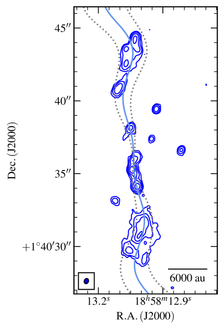
Figure 74: A radio contour map of G35.20$-$0.74N with a fitted jet model overlaid (light blue line), with the derived, minimum jet opening angle defined by the grey, dotted lines. Contour levels are the same as in Figure 24.

D.2.3 G035.1992$-$01.7424

Our RMS source is also known as the UCHii region, W48A, located in the W48 massive-star forming complex. Rygl et al. (2014) detected 3 FIR clumps towards the W48 region, one (H1) centred on the UCHii region and the other two, H2 and H3, located $16\arcsec$ and $63\arcsec$ to the west respectively. Both H1 and H2 have one $2.3{\rm\thinspace mm}$-core each, named H1a and H2a respectively, while H3 has two $2.3{\rm\thinspace mm}$-cores (H3a and H3b). Clump H2 was associated with methanol, hydroxyl and water maser activity, while clump H3 displayed a roughly north-east to south-west outflow traced by the CO ($3-2$) transition. Ultimately this work concluded that sequential star formation from (in order of most to least evolved) H1, to H2 and lastly to H3 explained their observations, with H2 bordering the UCHii’s photo-dissociation region (PDR) and therefore being pressured into collapse by the expanding Hii region. Most recently, $22{\rm\thinspace GHz}$ radio images employing $uv$-cuts of $>320\mathrm{k}\lambda$ by Masqué et al. (2017) resolved out much of the emission and detected a compact source at $\alpha\,(\mathrm{J2000})=19\hbox{$\rm{}^{s}$}01\hbox{$\rm{}^{m}$}46.46\hbox{$\rm{}^{s}$}$, $\delta\,(\mathrm{J2000})=01\degr 13\arcmin 23.6\arcsec$ (centre of W48A) with a flux of $5.24\pm 0.14{\rm\thinspace mJy}$ and deconvolved size of $(67\pm 3{\rm\thinspace mas})\times(39\pm 3{\rm\thinspace mas})$, at a position angle of $131\pm 5\degr$.

At C-band we detect a cometary UCHii, W48A, which limits the image in dynamic range due to its extended, bright emission. When moving to Q-band, the lack of short $uv$-spacings filtered out much of the extended structure and we detect partially resolved out emission at the location of the cometary Hii region’s bow shock. Further to this, we detect a compact source roughly at the Hii region’s geometric centre (i.e. at the location of the compact source detected by Masqué et al., 2017). From the K-band, radio flux previously recorded by Masqué et al. (2017), we derive a spectral index of $-0.11\pm 0.17$ with no change in deconvolved position angle or size (which makes the hypothesis of an ionized jet unlikely). From the models of a spherical, ionized wind (Panagia & Felli, 1975), this looks like an unlikely candidate for an ionized, stellar wind. To investigate this possibility however, from the measured flux at $44{\rm\thinspace GHz}$ of $4.84\pm 0.19{\rm\thinspace mJy}$, we infer a mass loss rate of (assuming $v=3000\hbox{${\thinspace\rm{\rm\thinspace km}{\rm\thinspace s}^{-1}\,}$}$) of $5.6\times 10^{-5}\hbox{${\rm\thinspace M_{\odot}}$}{\rm\thinspace yr}^{-1}$ (Wright & Barlow, 1975). From the models of Vink et al. (2001), we can infer a mass loss rate expected for a source of given luminosity/mass. For W48’s luminosity of $1.5\times 10^{5}\hbox{${\rm\thinspace L_{\odot}}$}$ we expect a mass loss rate of $\sim 2.5\times 10^{-6}\hbox{${\rm\thinspace M_{\odot}}$}{\rm\thinspace yr}^{-1}$ at best, which is around 20 times too small, compared to our measured flux at $44{\rm\thinspace GHz}$, which consequently rules out the stellar wind picture. With the calculated, optically-thin, spectral index, we can accurately calculate an emission measure of $(1.32\pm 0.14)\times 10^{9}{\rm\thinspace pc}{\rm\thinspace cm}^{-6}$, an average electron density of $(1.24\pm 0.14)\times 10^{6}{\rm\thinspace cm}^{-3}$ and a B1 type ($7600\hbox{${\rm\thinspace L_{\odot}}$}$, $11\hbox{${\rm\thinspace M_{\odot}}$}$) powering star, assuming it is a small Hii region. Considering W48A is powered by a star (or cluster) with a bolometric luminosity of $170000\hbox{${\rm\thinspace L_{\odot}}$}$, we can say that A is not powering the overall region. Therefore we deduce A to be a candidate, gravitationally-trapped Hii region, since half the major axis size ($106\pm 20{\rm\thinspace au}$) is smaller than the gravitational radius ($r_{g}=122{\rm\thinspace au}$ for $M_{\star}=11.3\hbox{${\rm\thinspace M_{\odot}}$}$).

Source B has no obvious K-band, or WISE $3/4{\rm\thinspace\upmu m}$ counterpart though we can not pass comment for longer wavelengths due to saturation of the WISE images at $12{\rm\thinspace\upmu m}$ and $22{\rm\thinspace\upmu m}$. Although not detected at C-band, we establish a dynamic range limited, $4\sigma$, upper limit on its flux of $147{\rm\thinspace\upmu m}$ and therefore a lower limit on its spectral index of $\alpha>-0.16\pm 0.11$. Assuming no variability in the source, this would suggest a thermal object, likely a deeply embedded, extremely young YSO. With the limitations to radio interferometric imaging from W48A, K or Ku-band observations would likely be needed to adequately establish the spectral index of B and therefore provide a firmer classification.

A methanol maser was detected which is co-located with a reddened source in UKIDSS NIR imagery, however no continuum emission is detected in C (dynamic range limited) or Q-band (with $4\sigma$ upper flux limits of $158{\rm\thinspace\upmu Jy}$ and $112{\rm\thinspace\upmu Jy}$ respectively) images. This methanol maser is located within clump H2/core H2a from Rygl et al. (2014) and likely points to a young MYSO on account of its non-detection at radio wavelengths.

D.2.4 G037.4266+01.5183

López-Sepulcre et al. (2010) detect a N-S oriented molecular outflow in C¹⁸O$(2-1)$. Subsequently, Surcis et al. (2015) used VLBI to identify 19 CH₃OH maser spots divided into two groups, A and B, to the NW and SE of G37.43+1.51’s position. No clear velocity gradients were observed in either group. However, group A shared their velocity with the outflow’s blue lobe, thereby associating the maser emission with the N-S molecular outflow of López-Sepulcre et al. (2010).

We detect one Q-band, $\sim 0.5{\rm\thinspace mJy}$, point-like source offset $\sim 11\arcsec$ to the north east of the pointing centre, which coincides with both a mid-infrared (in WISE imagery) source and B at C-band. A CH₃OH maser spot is detected $\sim 0\aas@@fstack{\prime\prime}3$ NW of B, itself coincident maser group A from Surcis et al. (2015). Both maser groups from Surcis et al. (2015) are plotted (pink crosses) in Figure 26 for reference. Two more C-band sources are detected, A and C, which both have red, NIR counterparts. While B possesses a thermal spectral index of $1.16\pm 0.12$, A and C were not detected at $44{\rm\thinspace GHz}$ and we derive upper limits of $\alpha<0.59\pm 0.11$ and $\alpha<0.29\pm 0.06$, respectively. No physical dimensions could be deconvolved using imfit and therefore we can only classify these three sources as jet candidates.

D.2.5 G056.3694$-$00.6333

Near-infrared UKIDSS imagery shows a reddened point source at the centre of some nebulosity towards the south west and north of the point source.

At C-band we see a string-like morphology slightly offset to the reddened, UKIDSS point source. Considering this morphology, this is likely an ionized jet with lobes, however a lack of results from other wavelengths in the literature means we must classify this as a candidate. Due to its proximity to the near-infrared source, C is assumed to be the YSO where the base of the jet is located, while A, B and D are shock-ionized lobes associated to the jet’s flow. Ideally high-resolution mm-observations would help to establish which components are affiliated with cores to clarify the picture further. In the case that C is indeed a jet, while A, B and D are shock-ionized radio lobes, mm sources should only be associated to C.

D.2.6 G077.5671+03.6911

Near infrared 2MASS images show this object to be at the centre of a possible cluster. Previous ammonia and water maser observations failed to detect significant emission (Urquhart et al., 2011), unusual for our sample of MYSOs.

One source, unrelated to the MYSO, was detected $23\arcsec$ to the SE of the pointing centre in the C-band clean images, however nothing was detected at Q-band. Considering that it has no associated near or mid-infrared source, it is most likely extragalactic in origin though its non-thermal or thermal nature can not be constrained ($\alpha<0.25\pm 0.11$).

D.2.7 G078.8699+02.7602

Another well studied region in our sample containing 3 Herbig Ae/Be stars named BD$+40\degr 4124$, V$1686$ Cygni and V$1318$ Cygni. Observed in both optical and NIR regimes, it was determined that V1318 Cygni was composed of 3 separate optical sources dubbed north, middle and south (Aspin et al., 1994), of which ‘south’ was concluded to be a very young, intermediate-mass, Herbig Ae/Be star with a low-mass binary companion, ‘north’, separated by $\sim 5000{\rm\thinspace au}$ and connected via the diffuse optical source ‘middle’. At sub-mm wavelengths, V$1318$ Cygni is by far the dominant source (see Figure 22 of Sandell et al., 2011). Navarete et al. (2015) observed this region in both K-band continuum ($2.2{\rm\thinspace\upmu m}$) and $\mathrm{H}_{2}$ line ($2.122{\rm\thinspace\upmu m}$) NIR filters. They detected a bipolar outflow in shocked $\mathrm{H}_{2}$ emission consisting of 4 lobes (sources 1a, 1b, 1c and 1d) roughly aligned at a position angle of $\sim 150\degr$ and extending over a length of $0.78{\rm\thinspace pc}$. The approximate midpoint of these lobes is located at $\alpha\mathrm{(J2000)}=20\hbox{$\rm{}^{h}$}20\hbox{$\rm{}^{m}$}30.6\hbox{$\rm{}^{s}$},\,\delta\mathrm{(J2000)}=41\degr 22\arcmin 06\arcsec$. Two more lobes (2 and 3) of shock emission were detected $\sim 2\arcmin$ from their pointing centre (which coincides that of our observations) at a position angle of $10\degr$.

UKIDSS imagery shows 4 bright sources within $1\arcmin$ of our field centre (Figure 29), the most easterly two being separated from eachother by $\sim 5\arcsec$, displaying red NIR colours and coincident with V$1318$ Cygni’s ‘north’ and ‘south’ source from Aspin et al. (1994) respectively. A less reddened source can be seen $\sim 14\arcsec$ to their east (V$1686$ Cygni) and the brightest source, blue in colour, is located $\sim 40\arcsec$ to the NE (BD$+40\degr 4124$). At C-band we detect radio emission from all of these NIR sources (A, B, C and E), as well as from a NIR dark source located $47\arcsec$ NNW of the pointing centre with profiterole-like morphology (D). Only sources A, B and C are detected at Q-band.

Source A is clearly resolved at Q-band with dimensions of $(99\pm 6\times 50\pm 7){\rm\thinspace au}$ for the listed distance of $1.4{\rm\thinspace kpc}$, while possessing values for $\alpha$ and $\gamma$ of $1.41\pm 0.08$ and $>-0.54\pm 0.03$ respectively. Its deconvolved position angle of $-31\pm 6\degr$ aligns it with the shocked emission lobes, 1c and 1d, of Navarete et al. (2015). Source B is extremely low signal to noise ($3\sigma$ level at Q-band) and is listed as a Q-band detection on the basis of its coincidence with the corresponding C-band source but does remain consistent with the standard jet model of Reynolds (1986) whereby $\alpha=0.64\pm 0.23$ and $\gamma=-0.91\pm 0.26$, which also describes a stellar wind. Without more supporting evidence however, we must classify is as a jet candidate. Source C remains unresolved at both frequencies and we calculate a spectral index of $\alpha=1.12\pm 0.08$ for it, but given its bright, blue NIR colours it has clearly evolved past the MYSO stage. For D we determine it to be extragalactic on account of its IR dark nature mixed with a limit to its spectral index of $\alpha<0.41\pm 0.19$. Our radio object E is not detected at Q-band and we establish an upper limit on $\alpha$ of $<0.50\pm 0.13$ and although definitely galactic, its more specific nature can not be determined. Considering the fact that optical counterparts exist to these objects (apart from D), it is highly likely that some are Herbig Ae/Be stars. As for the bolometric luminosities of each object, based on correction for the more accurate distance of Rygl et al. (2012), we adopt $5972\hbox{${\rm\thinspace L_{\odot}}$}$ and $528\hbox{${\rm\thinspace L_{\odot}}$}$ for A and B respectively (from Aspin et al., 1994), while for C we adopt a luminosity of $1080\hbox{${\rm\thinspace L_{\odot}}$}$ (Lumsden et al., 2012).

D.2.8 G079.8855+02.5517

Previous $\,{}^{12}\mathrm{CO}\left(3-2\right)$ maps detect an outflow with red and blue lobes along a position angle of $\sim 120\degr$ and roughly centred on the RMS source G079.8855+02.5517B (Gottschalk et al., 2012).

Within the RMS database, our C-band and Q-band detected source C is designated as G079.8855+02.5517C, while our Q-band-only source B1/B2 corresponds to RMS source G079.8855+02.5517B (the more luminous of the two by an order of magnitude). None of our sources are detected in UKIDSS, but C and B1/B2 are strongly saturated in GLIMPSE images apart from at $3.5{\rm\thinspace\upmu m}$. With a separation of just $97\pm 8{\rm\thinspace au}$ ($69\pm 4{\rm\thinspace mas}$ at a distance of $1400\pm 80{\rm\thinspace pc}$), B1 and B2 are likely a young binary system. Considering that B2 is elongated along a position angle of $131\pm 15\degr$, parallel with the molecular outflow observed by Gottschalk et al. (2012), we believe that it is an ionized jet whose flux is contributed to by dust emission (hence the steep spectral index of $\alpha>1.6\pm 0.1$).

Other detected emission in the field is the C-band source E (outside the Q-band primary beam) and Q-band source D. Since E has no near or mid-infrared counterpart, its most likely classification is extragalactic, while source D, with its steep ($\alpha>1.6\pm 0.1$) thermal spectral index and mid IR-dark appearance, is most probably a YSO at the beginning of its evolution.

D.2.9 G081.8652+00.7800 (W75N)

W75N is arguably the most well-studied region of our sample. Our C-band field of view encompasses 3 significant objects, one being an Hii region (RMS designation G081.8789+00.7822), another being the string of radio lobes (Carrasco-González et al., 2010) with confusing outflow morphology (Shepherd et al., 2003) and the last being a reddened MIR source (RMS designation G081.8652+00.7800) to the SW of the well studied radio object. The string of 5 radio lobes is oriented at a position angle of $\sim 170\degr$ from the clean maps of Carrasco-González et al. (2010) who determined their source VLA3 to be a thermal jet ($\alpha=0.6\pm 0.1$) powering the Herbig-Haro object, Bc, with the natures of VLA1, VLA2 and VLA4 uncertain. Significant radio flux variability was detected towards Bc over the period encapsulating all of their studied, archival observations ($\sim 13{\rm\thinspace yr}$).

At both C and Q-bands we detect an unresolved source dubbed ‘A’ which is coincident with the RMS source G081.8652+00.7800 and possesses a spectral index of $\alpha=1.00\pm 0.08$ indicative of thermal free-free emission. Upper limits on A’s physical dimensions of $(<50\times<24){\rm\thinspace au}$ are established from the higher frequency images indicating an extremely compact source. As a result, we can only classify this object to be a jet candidate as both its spectral index and extremely small dimensions lend themselves to interpretation as a small HCHii.

Approximately $24\arcsec$ to the NE of A we detect at least 9 sources in the C-band maps and 3 in the Q-band images. These form the well-studied jet/lobes of the W75N region and we report VLA5, VLA6 and VLA7 to be new sources previously undetected. VLA 1 is elongated at a position angle of $\sim 80\degr$, which is parallel with the large CO outflow reported in Shepherd et al. (2003), however imfit requires a two-component model at C-band, one for the central ‘core’ and the other for the more elongated emission to the north-east. VLA1’s ‘core’ is also detected at Q-band and has a spectral index of $\alpha=0.19\pm 0.06$. For the elongated emission we calculate $\alpha<-1.21\pm 0.07$. The accuracy of this result is debatable considering resolving out effect at Q-band and accurate deconvolution of VLA1 into two sources at C-band. Due to its strong alignment with an outflow, but uncertain spectral indices we assign in the classification of jet candidate.

VLA2 possesses values for $\alpha$ and $\gamma$ of $0.11\pm 0.07$ and $-1.46\pm 0.12$ respectively, with deconvolved position angles of $\sim 20\degr$ at both frequencies. From our analysis alone, and given the confusing picture of outflow and low signal to noise, we would classify VLA2 as a jet candidate. However considering the work by Carrasco-González et al. (2015), who observed the ‘onset of collimation’ for the thermal jet associated to VLA2, this radio object is definitively classified as a jet.

VLA4 is seen to possibly be another lobe of shocked emission by Carrasco-González et al. (2010) who required longer time baselines to see if proper motions were significant or not. Taking advantage of the larger time baselines between our $5.8{\rm\thinspace GHz}$ and their 2006, $8.46{\rm\thinspace GHz}$ observations we derive proper motions of $0.13\pm 0.04\arcsec$, or $126\pm 42\hbox{${\thinspace\rm{\rm\thinspace km}{\rm\thinspace s}^{-1}\,}$}$, at a position angle of $-178\pm 24\degr$. We believe that due to the $>3\sigma$ detection of this proper motion, this source is another radio lobe induced by jet shocks.

VLA5, VLA6 and VLA7 all fall well below the detection thresholds of previous radio observations and are both unresolved (VLA5) and distinctly extended (VLA6 and VLA7) in their morphology. Considering the overall morphology of the region, we assume these sources to be radio lobes, much like VLA4, Bc and Bc2, as the result of jet shocks.

The source W75NBc was detected to have proper motions of $\sim 220\pm 70\hbox{${\thinspace\rm{\rm\thinspace km}{\rm\thinspace s}^{-1}\,}$}$ by Carrasco-González et al. (2010), however the positions they catalogue for source Bc assume that our sources W75NBc and W75NBc2 (see Figure 31) are one and the same. Therefore to recalculate proper motions using our data, we used a deconvolved position derived from imfit assuming Bc and Bc2 to be the same source. It is important to note that we use the same phase calibrator ($\mathrm{J}2007+4029$) as that of Carrasco-González et al. (2010). At $5.8{\rm\thinspace GHz}$, this gives a 2012 epoch position of $\alpha\mathrm{(J2000)}:20\hbox{$\rm{}^{h}$}38\hbox{$\rm{}^{m}$}36.5525\hbox{$\rm{}^{s}$},\,\delta\mathrm{(J2000)}:42\degr 37\arcmin 31.4585\arcsec$ (with uncertainties in position of $24.9$ and $9.8{\rm\thinspace mas}$ in $\alpha\mathrm{(J2000)}$ and $\delta\mathrm{(J2000)}$ respectively) translating to a proper motion of $0.12\pm 0.05\arcsec$ ($\theta_{\mathrm{PA}}=161\pm 27\degr$) or $114\pm 46\hbox{${\thinspace\rm{\rm\thinspace km}{\rm\thinspace s}^{-1}\,}$}$ for the more accurate distance of $1.32\pm 0.11{\rm\thinspace kpc}$ from Rygl et al. (2010) ($173\pm 69\hbox{${\thinspace\rm{\rm\thinspace km}{\rm\thinspace s}^{-1}\,}$}$ using the distance of $2{\rm\thinspace kpc}$ adopted by Carrasco-González et al. (2010)). Considering this evidence for proper motions in both current and previous data, Bc2/Bc are classified as lobes representing the shocked surfaces of an ionized jet impinging upon its surroundings.

We also detect (C-band only) the Hii region (RMS designation G081.8789 +00.7822) whose material stretches across a region approximately $9.5\times 8.6\arcsec$ in angular size, or $0.064\times 0.058{\rm\thinspace pc}$, classifying it as an ultracompact Hii region. Considering its flux, assuming optically thin emission and using the models of Davies et al. (2011) we estimate it to have a bolometric luminosity (from its derived Lyman flux) of $6600\hbox{${\rm\thinspace L_{\odot}}$}$, mass of $11\hbox{${\rm\thinspace M_{\odot}}$}$ and therefore equivalent ZAMS type of B1. However, it must be noted that this is a lower-limit on both its flux and spatial extent due to potential spatial-filtering on these scales.

D.2.10 G083.7071+03.2817

Apart from galactic plane surveys, no previous significant observations targeting this MYSO exist in the literature. UKIDSS NIR images show extended nebulosity in a bipolar configuration, characteristic of cavities, at a position angle of $\sim 120\degr$ and more diffuse emission to the south west.

Towards this source we detect two C-band radio objects, A and B, and one Q-band source coincident with A. Source A is resolved with dimensions of $(0.237\pm 0.029\times 0.045\pm 0.061)\arcsec$ at $118\pm 9\degr$ and $(0.044\pm 0.01\times 0.012\pm 0.01)\arcsec$ at $111\pm 18\degr$ at C and Q-bands respectively. In turn we calculate spectral index values of $\alpha=0.47\pm 0.07$ and $\gamma=-0.83\pm 0.13$, in line with the models of Reynolds (1986) and A is therefore a thermal jet, especially given its alignment with NIR reflection nebulae in UKIDSS images (see left panel of Figure 32). Source B has an upper limit to its spectral index of $\alpha<-0.43\pm 0.04$ and, considering its unresolved dimensions at C-band and position angle with respect to A of $\sim-140\degr$ (i.e. perpendicular to A’s major axis), is most likely extragalactic in origin.

D.2.11 G084.9505$-$00.6910

Near infrared RGB images from UKIDSS show a well defined example of a bipolar reflection nebulae at a position angle of $\sim 120\degr$, centred on the MYSO, however no other previous targeted observations of this object are present in the literature.

At Q-band we detect one source, B, which is not resolved using imfit but does appear slightly elongated along a position angle of $\sim 120\degr$, parallel to what appears to be reflection nebulae (likely cavity walls) in UKIDSS imagery (left panel, Figure 33). At C-band no continuum source is detected coincident with the B, but a methanol maser is detected whose imfit derived position is offset to B’s Q-band peak by $\sim 0.8\arcsec$. Without further information we classify this to be a jet candidate, especially given its unusually steep (but still consistent with the models of Reynolds, 1986) spectral index of $\alpha>1.25$ suggesting flux contribution from dust emission. One source is detected only at C-band, A, which is outside of the Q-band primary beam and so no further analysis can be conducted leaving it with an unknown classification. However, it does not have either a UKIDSS (NIR) or WISE (MIR) counterpart meaning it is likely extragalactic.

D.2.12 G094.2615$-$00.4116

A knot of $\mathrm{H}_{2}$ $2.122{\rm\thinspace\upmu m}$ emission is detected to the SE of our source A1 (source 1 of A from Varricatt et al., 2010) and associated to a molecular outflow oriented NW to SE at an angle of $141\degr$ (Fontani et al., 2004).

We detect 3 sources within $50\arcsec$ of the pointing centre, A1, A2 and B. Source B is only detected at C-band, does not have an NIR counterpart and, from WISE imagery, probably does not have a MIR counterpart either (its position is on the limit of source confusion). Therefore B is classified as extragalactic in origin. A1 has both a C-band and Q-band detection inferring a spectral index of $\alpha=0.47\pm 0.19$, however no value for $\gamma$ could be obtained due to the relatively low ($5\sigma$) SNR at Q-band. Considering A1’s obvious elongation at C-band, apparent NIR cavities oriented at the same position angle and a parallel outflow, we classify it as a thermal jet. A2 is likely to be a lobe associated to A1’s jet, produced via shock emission. However its extended morphology ($1800\pm 400{\rm\thinspace au}$ by $1000\pm 800{\rm\thinspace au}$) and unknown MIR status make it a possibility that it is a small Hii region of a B3, ZAMS-type star (mass of $\sim 8\hbox{${\rm\thinspace M_{\odot}}$}$, for the calculated value $\log(\mathrm{N_{i}})=44.23\pm 0.09$, or $\mathrm{L}_{\star}=2300\pm 180\hbox{${\rm\thinspace L_{\odot}}$}$, from the models of Davies et al., 2011).

D.2.13 G094.3228$-$00.1671

Knots of H₂, $2.122{\rm\thinspace\upmu m}$ emission were detected by Navarete et al. (2015) and classified to be bipolar in distribution. Their orientation with respect to the RMS source are at position angles of $355\degr$, $185\degr$, $290\degr$ and $165\degr$ for H₂ lobes 1a, 1b, 1c and 1d respectively.

At both frequencies we detect an unresolved radio source designated as A $\sim 2\arcsec$ to the NW of the pointing centre and coincident with the reddened NIR source apparent in the left panel of Figure 35. At Q-band, A’s position is separated from that at C-band by $0.18\arcsec$ at a position angle of $107\degr$, however the positional accuracy code of the Q-band phase calibrator is ‘C’ and therefore we can not say if this offset is real. We derive a spectral index of $\alpha=1.19\pm 0.14$ between C and Q-bands, with an upper limit on the physical size of the emission at Q-band of $<(114\times 40){\rm\thinspace au}$. Due to the unresolved nature of the radio source, it can not be determined if the emission is parallel, or perpendicular, to the previously recorded outflow axes from Navarete et al. (2015). We therefore classify A as a jet candidate.

D.2.14 G094.4637$-$00.8043

Smith & Fischer (1992) used near-infrared line and continuum observations to show that activity from multiple jets is likely present in this region considering the wide range in outflow axes seen in their H₂, $2.12{\rm\thinspace\upmu m}$ images. More recent H₂ line observations (Navarete et al., 2015) showed 5 distinct regions of emission, with what appears to be 2 bipolar outflows at position angles of $355/180\degr$ (1a, 1b) and $210/30\degr$ (2a, 2b), and a monopolar outflow (3a) at a position angle of $-60\degr$. The monopolar outflow is also aligned with the obvious NE/SW bipolar reflection nebula in NIR images, and the 2a/2b outflow was aligned with another, fainter, NIR reflection nebula (see left panel of Figure 36).

In standard images with a robustness of $0.5$ (Figure 36), source A at C-band is coincident with A and A2 at Q-band, with an average spectral index (combining the two Q-band fluxes) of $\bar{\alpha}=0.65\pm 0.10$, typical of ionised jets. However considering their separation of $1090\pm 170{\rm\thinspace au}$ ($202\pm 2{\rm\thinspace mas}$ at $5.36\pm 0.84{\rm\thinspace kpc}$) and current theoretical ranges of jet launching radii between $10-100{\rm\thinspace au}$, we believe that A1 and A2 are close binaries. Imaging the C-band data with a more uniform robustness of $-2$ (increasing the effective resolution) shows that C-band source A is most likely the same source as Q-band source A, while A2 appears more separate from the C-band lobe. Using this approach, A’s spectral index is derived to be $0.39\pm 0.09$, while for A2 it is calculated to be $\alpha>1.61\pm 0.09$ (calculated with C-band flux’s $3\sigma$ upper-limit). Both A and A2 are roughly aligned with components B, D and E at a position angle of $\sim 45\degr$, for which we calculate spectral index upper limits of $<0.0$, $<0.4$ and $<0.5$ respectively. Component C is detected at both bands and has a jet-like spectral index of $0.86\pm 0.09$, and although imfit was unable to deconvolve any sizes, at Q-band the emission looks slightly elongated along a position angle of $\sim 10\degr$.

Comparing our results to those of Navarete et al. (2015) who detect three distinct directions of collimated outflow, we detect 3 heavily thermal components (A, A2 and C). Although no definitive spectral indices could be deduced for B, D or E, we believe that due to their alignment with A, they represent shocked surfaces of optically thin and/or non-thermal emission from a thermal jet ejected at a position angle of $\sim 45\degr$ from A. The H₂ bipolar outflow components 2a and 2b are aligned along this axis and therefore likely more distant jet-shock features. A2 is likely a close binary to A, though its possible association with an outflow is unknown. The thermal jet at C also has a $4\sigma$ component to its WNW, in line with the monopolar outflow 3a, however without more information, we can not be sure as to C’s exact nature. We therefore classify A to be a jet with lobes and both A2 and C as jet candidates.

D.2.15 G094.6028$-$01.7966

More popularly known as V645 Cygni, this object has a rich observational history. Notably Murakawa et al. (2013) detected Br$\gamma$ emission with a P-Cygni profile and a blue absorption feature in $\mathrm{HeI}$ strongly shifted in velocity by $-800\hbox{${\thinspace\rm{\rm\thinspace km}{\rm\thinspace s}^{-1}\,}$}$. This implies fast moving gas in the line of sight towards us. Modelling CO bandhead emission detected during their K-band spectroscopic analysis showed that the accretion disc in the system was almost pole-on, reinforcing the theory that a stellar wind/ionized jet was oriented towards the observer. Previous to this, a bipolar CO $J=3-2$ outflow was detected by Schulz et al. (1989), centred on V645 Cygni.

At both C-band and Q-band we detect a compact source, ‘A’, at the pointing centre. Methanol maser emission is also seen coincident with A. Although no physical dimensions could be deconvolved, we derive a spectral index for the emission of $0.49\pm 0.08$. Considering the observational history and compatibility with either a disc-wind, or a thermal jet, we classify this object as a jet candidate.

D.2.16 G100.3779$-$03.5784

This YSO was observed by Moscadelli et al. (2016) at frequencies of $6.2$, $13.1$ and $21.7{\rm\thinspace GHz}$ with the VLA in its A-configuration. They detect a compact source which is slightly resolved at the upper two frequency bands with a spectral index of $\alpha=0.84\pm 0.25$. Previously Anglada & Rodríguez (2002) also observed the same object (their VLA2, which also had a NW extension to its emission), as well as another radio lobe $\sim 10\arcsec$ to the south (VLA1). In UKIDSS imagery, a red source is coincident with the previous radio detection, which appears extended in the N-S direction.

At C-band we detect two sources, which we designate A and B. Source A coincides with VLA2 from Anglada & Rodríguez (2002) and therefore the same radio source from Moscadelli et al. (2016), for which we derive a spectral index of $\alpha=0.79\pm 0.12$, in line with that estimated previously. Combining our data with that from Moscadelli et al. (2016), we derive a more accurate spectral index of $\alpha=0.80\pm 0.10$ (neglecting their C-band result due to poor image quality). Although no deconvolved dimensions could be established, source A looks extended in an E-W direction in both C and Q-band images in agreement with $3.6{\rm\thinspace cm}$ morphology seen by Anglada & Rodríguez (2002). Source B, which is extended at C-band, is not detected likely owing to an optically thin spectral index and/or the loss of flux with the smaller synthesised beam. Due to the near IR colours presented in UKIDSS RGB images, we classify B as an Hii region. Although jet-like, without morphological information source A is classified as a jet candidate.

D.2.17 G102.8051$-$00.7184

The RMS survey catalogues three red MSX sources, G102.8051$-$00.7184A, B and C, within $15\arcsec$ of eachother, with bolometric luminosities of $2300\hbox{${\rm\thinspace L_{\odot}}$}$, $2300\hbox{${\rm\thinspace L_{\odot}}$}$ and $1300\hbox{${\rm\thinspace L_{\odot}}$}$ respectively. Four millimetric sources were found by Palau et al. (2013), with their MM2 being the only possibly massive ($2-10\hbox{${\rm\thinspace M_{\odot}}$}$) core in the region ($22\hbox{$\rm{}^{h}$}19\hbox{$\rm{}^{m}$}08.974\hbox{$\rm{}^{s}$}$, $56\degr 05\arcmin 02.97\arcsec$) and the only one driving a CO$(2-1)$ bipolar outflow (position angle of $-20\degr$). Fontani et al. (2004) detected a CO$(1-0)$ outflow at a position angle of $\sim 10\degr$ with the NE blue lobe coincident with both [FeII] and H₂ line emission indicative of shocks from protostellar outflows. GLIMPSE imagery shows a reddened, extended source with all the typical characteristics of an Hii region approximately $15\arcsec$ NE of G102.8051$-$00.7184B and with a luminosity of $660\hbox{${\rm\thinspace L_{\odot}}$}$ (from the RMS survey).

At C-band we detect one source, however it is not coincident with any reddened, MIR source in GLIMPSE, with colours (in near and mid-infrared images) more attributable to a more evolved phase. Further to this, no corresponding source was detected at Q-band, establishing an upper limit to the spectral index of $<0.61\pm 0.15$.

D.2.18 G103.8744+01.8558

Previous PdBI (2mm) and VLA observations (multiple frequencies) detect 6 mm-cores associated to the IRAS source (22134+5834), one of which (MM2) is coincident with a detected UCHii region, VLA1 (Wang et al., 2016) which was calculated to be powered by a B1 ZAMS type star. Of the 6 detected cores, MM1 was both the brightest and heaviest with a 2mm flux of $9.3\pm 2.0{\rm\thinspace mJy}$ and inferred mass of $6.1\pm 1.3\hbox{${\rm\thinspace M_{\odot}}$}$.

At C-band, we detect 5 sources which we label A, B, C, D and E, of which only A is detected at Q-band. In terms of C-band radio flux, A is the brightest and a spectral index of $\alpha=-0.42\pm 0.12$ is derived for A, however we believe that this is due to resolving out effects at Q-band. This is supported by the decrease in deconvolved major axis length with frequency (Hii regions should not change in size). From the optically thin (verified by the previous observations of Wang et al., 2016) $5.8{\rm\thinspace GHz}$ emission, the models of Davies et al. (2011) predict a bolometric luminosity of $4200\hbox{${\rm\thinspace L_{\odot}}$}$. In comparison to the infrared derived bolometric luminosity of $6800\hbox{${\rm\thinspace L_{\odot}}$}$, we believe that the difference of $2600\hbox{${\rm\thinspace L_{\odot}}$}$ is supplied by the other 5 cores in the vicinity, most of which comes from MM1, which is coincident with our source B. Our only other detected radio source with a corresponding mm-core is C which is associated to MM4 of Wang et al. (2016). From the general morphology, we believe D, E and F (which have no IR or mm counterparts) are shock sites whereby ejected material from B is impacting the surrounding dust/gas. We classify B as a jet with lobes on the basis of its elongated morphology along a position angle of $114\degr$ which is aligned with the string of lobes, D, E and F. Although source C may be a YSO, however its exact classification is unknown and we therefore classify it as a jet candidate.

D.2.19 G105.5072+00.2294

Molinari et al. (2002) detected a $0.12\pm 0.03{\rm\thinspace mJy}$ $3.6{\rm\thinspace cm}$ radio source (VLA1) coincident with a ‘ring’ of HCO${}^{+}(1-0)$ line emission towards the MSX source. A CO $J=2-1$ molecular outflow has also been observed whose emission peaks $\sim 10\arcsec$ to the NW of the MSX position (Zhang et al., 2005). A definitive position angle for the outflow is difficult to establish with the red lobe elongated at a position angle of $\sim 90\degr$ and the blue lobe at an angle of $-160\degr$. H₂ 2.122${\rm\thinspace\upmu m}$ observations by Varricatt et al. (2010) showed three distinct patches of shock emission aligned along a position angle of $\sim 15\degr$ and separated from the infrared source by $20\arcsec$ to the NNW.

One, elongated radio source is detected at both frequencies (A) with values for $\alpha$ and $\gamma$ of $1.02\pm 0.13$ and $-1.05\pm 0.44$ respectively. Deconvolved position angles for the major axis agree at both frequencies with a value of $\sim 110\degr$ parallel with the NIR reflection nebulae of the outflow cavities apparent in the left panel of Figure 41. Confusingly this position angle does not align well with the H₂ emission or blue CO $J=2-1$ lobe, but is parallel with the elongated red CO $J=2-1$ emission. Assuming the radio source is a jet, it is possible that the outflow axis has precessed towards the west considering the trail of H₂ emission and the elongation of the radio source at $110\degr$. However, further observations will be needed to clarify this picture and A is assigned a classification of jet candidate.

D.2.20 G107.6823$-$02.2423A

Previous near-infrared spectroscopic observations detected both Br$\gamma$ and [Feii] emission (Cooper et al., 2013) with a slit positioned over both G107.6823$-$02.2423A and its neighbouring Hii region G107.6823$-$02.2423B. While the strong Br$\gamma$ is attributable to the Hii region, the $1.64{\rm\thinspace\upmu m}$ [Feii] emission is a consequence of shocked material, possibly attributable to jet activity. Diffuse $2.122{\rm\thinspace\upmu m}$ H₂ emission is detected by Navarete et al. (2015) over ranges in position angle from the central source of $210-240\degr$ and $250-360\degr$.

Coincident with two NIR 2MASS sources are two C-band detections, one of which is extended and resolved out (Hii, coincident with G107.6823$-$02.2423B) and the other (A) which is located at the pointing centre and is also detected at Q-band. For the latter we derive a spectral index of $\alpha=1.15\pm 0.21$, however the source is point-like at all frequencies (which may be due to the low SNR or it possessing a true, unresolved nature). Due to the lack of further information, this source is classified as a jet candidate.

D.2.21 G108.1844+05.5187

One of the nearest objects in our sample at a distance of $0.776^{+0.104}_{-0.083}{\rm\thinspace pc}$ (Rygl et al., 2010), Beltrán et al. (2006) detected a $\mathrm{CO}$ outflow at a position angle of $140\degr$ centred on their source, OVRO 2 (mass of $14.2\hbox{${\rm\thinspace M_{\odot}}$}$), with the (weak) red lobe towards the SE and (strong) blue to the NW. Surcis et al. (2013) used polarimetric, VLBI observations to detect 29 methanol masers aligned along the same position angle ($145\pm 11\degr$) as the molecular outflow and derived a magnetic field position angle of $9\pm 15\degr$. For this source we adopt a bolometric luminosity of $873\hbox{${\rm\thinspace L_{\odot}}$}$ based on the luminosity found by Sugitani et al. (1989) of $1100\hbox{${\rm\thinspace L_{\odot}}$}$, corrected for the more recent distance found by maser parallax (Rygl et al., 2010).

Towards the mm-emission of previous observations, we detect source A to be coincident with OVRO 2 from Beltrán et al. (2006). The emission is elongated along a position angle of $42\pm 18\degr$ and $42\pm 7\degr$ at C (which is embedded in diffuse emission) and Q-band respectively, giving an offset to the magnetic field position angles of $33\pm 18\degr$. Considering that the radio emission is almost perpendicular ($82\pm 18\degr$) to the outflow, which itself is significantly offset to the magnetic field direction, a confusing picture is established. However, given the overwhelming evidence for an outflow from source A (and the elongation of a reddened 2MASS source along the outflow axis), we believe that the Q-band emission is tracing a disc of dimensions $(61\pm 12)\times(12\pm 8){\rm\thinspace au}$. We therefore conclude that source A traces an ionized jet (candidate) at C-band, but is dominated by disc emission at Q.

Source B is not coincident with any near or mid-infrared emission, was not detected at Q-band (though was located far out in the primary beam) and does not display any mm-emission at all. Considering these facts, we conclude it to be extragalactic in origin.

D.2.22 G108.4714$-$02.8176

Navarete et al. (2015) detect a bipolar H₂ outflow at a position angle of $15\degr$ centred on a reddened 2MASS point source (left panel of Figure 44).

We detect one component at both bands, centred on the red 2MASS source, with a spectral index of $\alpha=0.55\pm 0.16$. While not at C-band, it is resolved at Q-band ($\gamma>-0.77\pm 0.35$), with a major axis aligned along a position angle of $\theta_{\mathrm{PA}}=101\pm 25\degr$, perpendicular to the H₂ outflow’s direction. With the spectral index indicative of a typical ionised jet or disc wind, we classify this as a disc wind on the basis of its Q-band elongation perpendicular to the established outflow. It is worth noting that the C-band image shows a slight elongation at a position angle parallel with the H₂ bipolar outflow.

D.2.23 G108.5955+00.4925A

Associated to the infrared source, IRAS 22506+5944, the RMS survey lists two more MYSOs within $60\arcsec$ of G108.5955+00.4925A, being G108.5955+00.4925B and G108.5955+00.4925C, owing to this being a cluster of at least 15 members (Kumar et al., 2006). GLIMPSE imagery shows diffuse $8{\rm\thinspace\upmu m}$ emission centred on G108.5955+00.4925C, characteristic of a Hii region, however it is categorised as an MYSO based on NIR spectral features (Cooper et al., 2013). G108.5955+00.4925A itself is centred on a green (but not extended) MIR object and G108.5955+00.4925B is centred on a reddened MIR compact source. Previous ${\rm\thinspace mm}$ observations (Su et al., 2004) detected a $3{\rm\thinspace mm}$ core, which appeared to be driving a bipolar CO outflow at a position angle of $\sim 90\degr$ but was not positioned over any of the three RMS MYSOs.

Three C-band radio sources were identified from the radio clean maps, however we did not detect any at Q-band. In light of the RMS survey’s naming schemes, we dub them B, C (G108.5955+00.4925B and G108.5955+00.4925C respectively) and D (not in the RMS database). All are coincident with mid-infrared sources, however D’s source is not reddened and therefore is likely of a more evolved evolutionary status. Our source B has a very low flux ($30\pm 8{\rm\thinspace\upmu Jy}$), and therefore a non-restrictive upper limit to its spectral index of $\alpha<0.73\pm 0.14$. Without more information, we classify B to be a jet candidate. On the other hand, C is classified as a Hii region due to its extended morphology, coincidence with a diffuse MIR source and radio flux which matches that expected of a Hii region with a bolometric luminosity of $2700\hbox{${\rm\thinspace L_{\odot}}$}$ (Davies et al., 2011), which agrees with the $3000\hbox{${\rm\thinspace L_{\odot}}$}$ derived from infrared SED fitting. A CH₃OH maser was detected at $\alpha\,(\mathrm{J2000})=22\hbox{$\rm{}^{h}$}52\hbox{$\rm{}^{m}$}38.3110\hbox{$\rm{}^{s}$},\delta\,(\mathrm{J2000})=60\degr 00\arcmin 51.885\arcsec$ (with positional uncertainties of $7$ and $9{\rm\thinspace mas}$ in $\alpha$ and $\delta$ respectively) but was not coincident with any RMS source, or infrared/radio continuum source. However, it was coincident with the $3{\rm\thinspace mm}$ core/CO outflow detected by Su et al. (2004). It is therefore likely that this maser reveals the position of a deeply embedded, relatively unevolved MYSO, considering the already clustered environment towards this source.

D.2.24 G108.7575$-$00.9863

While GLIMPSE images are completely saturated, 2MASS (left panel of Figure 46) shows a reflection nebula centred on G108.7575$-$00.9863 with its diffuse emission extending over a position angle range of $225-280\degr$, with respect to the MYSO which lies at the heart of a cluster of $38$ members (Chen et al., 2009). NIR observations (Cooper et al., 2013) show a relatively featureless spectra, with only a weak Br$\gamma$ line present. Approximately $130\arcsec$ to the NNW is the classical Hii region, Sh2-152, which harbours a cluster and is a well studied object. Navarete et al. (2015) detect H₂ 2.122${\rm\thinspace\upmu m}$ emission dispersed widely over a wide area, including diffuse/knotted emission towards Sh2-152 and bipolar outflows centred on G108.7575$-$00.9863 and to the W and ESE of it. No obvious driving force can be determined for the source of the shocking material, though the obvious candidate is G108.7575$-$00.9863, especially due to its coincidence with the bipolar H₂ emission, BP1.

We report the detection of 5, compact C-band sources within $1\arcmin$ of the pointing centre (i.e. G108.7575$-$00.9863). These are labelled A$\rightarrow$E, of which A and B have near-infrared counterparts (NIRS 172 and NIRS 182 from Chen et al., 2009, respectively). Source A is also situated on a heavily saturated GLIMPSE source, is the only detection at Q-band within the primary beam, possesses a spectral index of $0.94\pm 0.09$ and remains unresolved at all frequencies. Without further information, we consequently classify it to be a jet candidate. Due to B’s reddened near infrared colours, it is determined to be a cluster member though its evolutionary status remains ambiguous without further information. Source C through E all suffer from the same classification issues of non-restrictive, thermal upper limits to spectral indices and lack of information at other wavelengths and we therefore classify them all to be of unknown nature. A methanol maser coincident with small 3$\sigma$ source $1.5\arcsec$ to the north of E is also detected suggestive of a well-embedded YSO.

D.2.25 G110.0931$-$00.0641

K-band images from 2MASS show diffuse emission to the south-east, east and north-east of a bright point source centred on G110.0931$-$00.0641’s position. A bipolar H₂ $2.122{\rm\thinspace\upmu m}$ outflow is detected at a position angle of $125\degr$ and centred on the MYSO (Navarete et al., 2015). Radio observations conducted in 2007 at $3.6{\rm\thinspace cm}$ ($8.33{\rm\thinspace GHz}$) using the VLA in its A-configuration detected 3 lobes of emission arranged along an axis at a position angle of $\sim 110\degr$ (Rodríguez et al., 2012). López-Sepulcre et al. (2010) detect a HCO${}^{+}(1-0)$ outflow at a rough position angle of $45\degr$ and elongated emission in C¹⁸O$(2-1)$ (tracing dense material) perpendicular to it. Both types of emission were centred on G110.0931$-$00.0641.

At C-band we detect 5 radio components named A1 (VLA3 from Rodríguez et al., 2012), A2, B (VLA2 from Rodríguez et al., 2012), C (VLA1 from Rodríguez et al., 2012) and D, all of which are within $3\arcsec$ of the pointing centre. Both B and C are detected at Q-band and B’s morphology is elongated in the direction of C. Spectral indices were therefore only established for B and C, and were calculated to be $0.34\pm 0.14$ and $-0.08\pm 0.16$ respectively, indicative of optically thin free-free emission. Components A1, A2, B and C are all approximately aligned on a position angle of $110\degr$, while D is located $2.5\arcsec$ to the NE of A1.

Under the assumption that A1, A2, B and C are all Hii regions, the sum of the radio flux-inferred bolometric luminosities of $(1.2\pm 0.1)\times 10^{4}\hbox{${\rm\thinspace L_{\odot}}$}$, is slightly under-luminous for that derived from SED fits of infrared data ($1.7\times 10^{4}\hbox{${\rm\thinspace L_{\odot}}$}$). However, B is optically thick and therefore under-luminosity is expected, meaning that a quadruple system of neighbouring Hii regions is still possible at this point. Considering the alignment with previously established outflows, proper motions and changes in physical size from C to Q-bands, an alternative explanation is that of a radio jet/lobe system. Considering the high-positional accuracy quality code of the phase calibrators used at C-band (J$2230+6946$) and Q-band (J$2250+5550$), for the optically thin radio lobe, C, any positional change between frequencies should be solely due to proper motions (which we do not expect to see in the Hii region case). For C, an angular shift of $67\pm 3{\rm\thinspace mas}$, at a position angle of $283\pm 5\degr$ (along the axis joining the lobes), is deduced from C to Q-bands corresponding to a proper motion of $1092\pm 226\hbox{${\thinspace\rm{\rm\thinspace km}{\rm\thinspace s}^{-1}\,}$}$ (using a distance of $4.70\pm 0.82{\rm\thinspace kpc}$ and $\Delta t=508\pm 52$ days). This is typical of observed velocities for radio lobes detected towards MYSOs and serves to strengthen the case that C is an optically-thin, shock-ionized lobe. On the basis of the excellent agreement of spectral indices with the models of Reynolds (1986), proper motions observed towards C and the general alignment of the radio lobes with outflows, we classify B as a radio jet with lobes (A1, A2 and C). As for D, in light of the Hii region-like infrared K-band morphology, we believe it is an extended Hii region whereby resolving out is starting to affect recovered flux/morphology at C-band and resulted in a non-detection at Q.

D.2.26 G111.2348$-$01.2385

Near-infared (2MASS) images show a point source embedded in a reflection nebula extending to the east of it. Beuther et al. (2002a) detected a CO $(2-1)$ molecular outflow oriented east to west. Previously, this source was observed by the VLA at both $8.44{\rm\thinspace GHz}$ and $43.4{\rm\thinspace GHz}$ by Garay et al. (2007), who observed a compact source centred on the MYSO’s location, with a spectral index of $1.1\pm 0.2$, and a large, cometary Hii region whose peak is located $15\arcsec$ to the north west. That work concluded the compact source to be a HCHii region around the MYSO, which was still undergoing accretion. Later $3.6{\rm\thinspace cm}$ ($8.33{\rm\thinspace GHz}$) radio observations using the VLA in its A-configuration detected one radio component elongated at a position angle of $97\degr$ with a line of 8 H₂O maser spots roughly perpendicular to it (Rodríguez-Esnard et al., 2014). Sub-mm observations show two cores in the continuum ($875{\rm\thinspace\upmu m}$), one centred on G111.2348$-$01.2385 and the other located $\sim 2\arcsec$ to its south west, with an east-west SiO$(8-7)$ outflow centred on G111.2348$-$01.2385 (Beuther et al., 2007) and another in the north east-south west direction, presumably from the other core.

At both frequencies we detect one radio lobe coincident with the NIR point source. A spectral index of $1.10\pm 0.07$ (in agreement with that calculated by Garay et al., 2007) is calculated, and interestingly the deconvolved dimensions of the emission show it to be elongated at a position angle of $173\pm 9\degr$ at Q-band (unresolved at C-band). This position angle is perpendicular to that derived by previous $8.33{\rm\thinspace GHz}$ observations of $97\degr$ (Rodríguez-Esnard et al., 2014) which, coupled with the steep spectral index, suggests that at Q-band, dust emission starts to dominate over the (perpendicular) ionized component. However, contrary to this, if we take fluxes from the variety of frequencies present in the literature, the spectral index remains steady across all bands. Considering the history of previous observations, an ionized jet may be located at the single radio component we detect, however it is equally likely the emission stems from a HCHii region. Without further radio information, we can not establish the dust’s flux contribution and therefore can not elucidate the nature of the radio object further. Consequently, we assign the classification of jet candidate to this object.

D.2.27 G111.2552$-$00.7702

Radio observations at $8.66{\rm\thinspace GHz}$ (Tofani et al., 1995; Sridharan et al., 2002) imaged a compact source at the position of G111.2552$-$00.7702 with time-variable flux. Later, higher resolution observations (Trinidad et al., 2006) showed the previous compact source (labelled I23139) and an unresolved $3.5{\rm\thinspace cm}$ source $0.5\arcsec$ to its SSW. I23139 was deduced to be an ionized jet on the basis of its spectral index ($0.64\pm 0.36$) and masers tracing an outflow (Goddi et al., 2005, who derived maser proper motions along a position angle of $\sim-70\degr$). Varricatt et al. (2010) showed that the MYSO is centred on a K-band source which is resolved as a binary (separation of $0.4\arcsec$) in their images. Further to this they also detected a H₂ $2.122{\rm\thinspace\upmu m}$ knot at a position angle of $65\degr$ from the MYSO. A molecular outflow was detected in CO $(2-1)$ but with no discernible outflow axis since the red and blue lobes lay on top of eachother (Beuther et al., 2002a), suggesting a head on orientation.

Within $1\arcmin$ of the pointing centre, we detect 5 compact, C-band radio objects, which we label A1, A2, B, C and D. Component A1 has a Q-band counterpart with a spectral index, between the two frequencies, of $\alpha=0.16\pm 0.12$. The spectral index may be steeper however considering A2’s close proximity at C-band which, when using imfit, can lead to flux being wrongly allocated from A2 to A1. Considering the spectral index previously found ($\alpha=0.64\pm 0.36$, Trinidad et al., 2006), this may indeed be the case. Because A1’s major axis and A2’s $\theta_{\mathrm{PA}}$, with respect to A1, is oriented at a position angle parallel to that of maser proper motions (Goddi et al., 2005) resulting from an outflow, we suggest A2 is a shock-excited lobe of emission, with the jet source located at A1. We therefore classify A1 as a thermal jet with lobes.

A CH₃OH maser is also detected offset from the continuum at C-band by $0.13\arcsec$ at a position angle of $-48\degr$. Components B and C appear to have near-infrared counterparts from 2MASS images, while D does not. However, because the spectral indices of these three components is not constrained, we must assign them an unknown classification. Further to those sources reported above, a $4\sigma$ source is detected $0.6\arcsec$ SW of A1 and coincident with I23139S (indicated to the south west of A1 by a $3\sigma$ contour in Figure 49). With an imfit derived flux of $15.5\pm 7.6{\rm\thinspace\upmu Jy}$ and in combination with the flux at $8.6{\rm\thinspace GHz}$ derived by Trinidad et al. (2006), we calculate a spectral index of $6.8\pm 1.5$, which is clearly not realistic. We therefore propose that I$23139$S is another time variable (over the $11{\rm\thinspace yr}$ period between their observations and ours) object.

D.2.28 G111.5671+00.7517

One of the best examples of a NIR reflection nebulae is seen in 2MASS images of this source (also known as NGC7548$-$IRS9), which extends towards the south west of the redenned MYSO. Previous $3.6$ and $1.3{\rm\thinspace cm}$ radio observations by Sánchez-Monge et al. (2008) detected two compact radio components at $1.3{\rm\thinspace cm}$ associated to NGC7548$-$IRS9. While their VLA3 is coincident with G111.5671+00.7517, VLA2 was offset approximately $5\arcsec$ to the west, yet both sources were coincident with K-band NIR (2MASS) point sources. At $3.6{\rm\thinspace cm}$, their images were affected by a bright, extended Hii region’s sibelobes from the NW resulting in a non-detection. Navarete et al. (2015) resolved a bipolar H₂, $2.122{\rm\thinspace\upmu m}$ outflow at a position angle of $\sim 155\degr$ with respect to the MYSO, and another in an east-west direction. Sub-mm observations of HCO⁺ and CO $(1-0)$ have shown two outflows, one coincident with the H₂ jet and driven by VLA2 (Sánchez-Monge et al., 2008) and the other associated to VLA3 and driven along a position angle of $\sim 70\degr$.

In our C-band images, we detect 5 radio components within $60\arcsec$ of G111.5671+00.7517, labelled, in order of distance from the centre, A (coincident with VLA3), C, B2, B1 and D. Of these 5 components, only A has a NIR or Q-band counterpart. The Q-band counterpart of A is distinctly elongated at a position angle of $19\degr$, pointing towards C, and has a spectral index of $0.87\pm 0.06$. Since there are no NIR source associated with C, B1 or B2 by inspection of the high-resolution ($\theta=0.4\arcsec$) RGB, J, H and K-band images of Mallick et al. (2014), we believe them to be shock-ionized lobes, especially given their optically thin spectral indices. From the morphology of the emission, we believe the jet is launched and collimated at A. On this basis we therefore classify A to be a jet with lobes. Also, considering the position angles of lobes B1, B2 and C with respect to A (in order of separation) of $214\degr$, $205\degr$ and $21\degr$ respectively, in conjunction with the wide angle reflection nebula at K-band, the molecular outflow at $70\degr$ and the current jet’s major axis defined by the Q-band data ($19\degr$), we believe A’s jet axis to be undergoing rapid, clockwise (on the plane of the sky) precession. Assuming a jet velocity of $500\hbox{${\thinspace\rm{\rm\thinspace km}{\rm\thinspace s}^{-1}\,}$}$ and inclination of $90\degr$ (i.e. jet lies in the plane of the sky) this indicates a shift of $12.5\degr$ over $23.2{\rm\thinspace yr}$, or a precession rate of $\sim 0.5\degr\,{\rm\thinspace yr}^{-1}$. This would also explain why the molecular outflow being driven from A is outflowing at a position angle of $70\degr$. As for source D, because of its non-detection and location on the edge of the Q-band’s primary beam, a non-restrictive upper limit of the spectral index was deduced ($\alpha<0.26\pm 0.11$) and therefore we classify as unknown in nature.

D.2.29 G114.0835+02.8568

Being a relatively unstudied object within our sample, the only relevant observations are those of Navarete et al. (2015) who observed a bipolar H₂ outflow along a rough north-south axis and centred on the MYSO’s position. In near infrared RGB images, the MYSO is centred on an extended (in the north west-south east direction), reddened source.

Only C-band observations of this field were observed in which we detect 5 radio sources, labelled A1, A2, B, C and D, of which A1 and A2 are spatially coincident with G114.0835+02.8568 and the only sources associated to a NIR point source. Component B looks spatially extended/resolved out and lies within the K-band nebulosity seen in 2MASS images, whereas C (the strongest source in the field) and D are located distinctly away from the central MYSO. For A1/A2, because of the lack of Q-band images, spectral indices can not be established and therefore either component could be a YSO, or a lobe of shocked emission. Without further information, we can not constrain the natures of the radio objects and therefore assign them all with an unknown classification.

D.2.30 G118.6172$-$01.3312

Aside from the usual surveys of the whole galactic plane, no observations towards this source are present in the literature. In 2MASS near-infrared images, the MYSO presents itself as a red source in a cluster of other, slightly less reddened, point sources. GLIMPSE images are verging on saturation at $8{\rm\thinspace\upmu m}$ over the MYSO’s position, with diffuse $8{\rm\thinspace\upmu m}$ (presumably PAH emission) to the north and north east spread across a wide area.

Unusually we only detect one source at Q-band which is not detected at C-band, therefore we establish a lower limit to the spectral index of $>1.59\pm 0.14$, which is unusually high for the sample in general. The radio source is just resolved with dimensions of $48\times 21{\rm\thinspace mas}$, corresponding to $134\times 56{\rm\thinspace au}$, with the major axis oriented at a position angle of $15\degr$. However, the errors on these derived quantities are large due to the low SNR of this source. Considering the lack of any data at other wavelength regimes, as well as at C-band, we classify this as a jet candidate.

D.2.31 G126.7144$-$00.8220

G126.7144$-$00.8220 is situated at the centre of a bipolar, near-infrared nebula aligned at a rough position angle of $-10\degr$, typical of outflow cavities. A $2.122{\rm\thinspace\upmu m}$ H₂ bipolar outflow centred on the MYSO and driven along a north-south axis $\theta_{\mathrm{PA}}\sim-10\degr$ was observed by Navarete et al. (2015). The same work also detected knots of H₂ emission to the west and north west. No other relevant, high-resolution observations exist in the literature for this object.

Centred on the reddened 2MASS object, we detect an elongated source at C-band, which splits into two Q-band sources (A and A2) separated by $0.15\arcsec$ ($\sim 110{\rm\thinspace au}$ at the RMS survey’s distance of $0.7{\rm\thinspace pc}$). We calculate an overall spectral index of $0.83\pm 0.05$ using the C-band flux for A and the combined fluxes of both sources at Q-band. For this object, two scenarios fit the radio data we have obtained. The first scenario is that the Q-band sources are a close binary of two YSOs, one of which is driving the previously detected $2.122{\rm\thinspace\upmu m}$ H₂ outflow. On the other hand, due to their combined, jet-like spectral index and small separation, this could in fact be a biconical jet, whereby we are seeing the direct emission from the launching site of the jet and counter-jet, with a launching radius of $55{\rm\thinspace au}$ (assuming symmetry). This second scenario is supported by the alignment of the two sources with the H₂ outflow, however it must be conceded that this may be a chance alignment. With the equal likelihood of both scenarios, we classify both objects as jet candidates.

D.2.32 G133.7150+01.2155

More commonly associated with the alias W3 IRS5, this is an extremely well studied object. Previous radio observations at K and Q-bands by van der Tak et al. (2005) detected 5 sources (labelled Q$1\rightarrow$Q$5$) at Q-band and 8 sources (labelled K$1\rightarrow$K$8$) at K-band. Of these, Q1/K2, Q2/K3, Q3/K4, Q4/K6, Q5/K7 and Q6/K5 were determined to be the same Q-band/K-band sources, with ranges in thermal spectral indices of $0.5\leq\alpha\leq 1.4$ determining them to by YSOs and therefore highlighting the tight clustered environment. Using speckle MIR imaging, the same work determined Q3/K4, Q4/K6 and Q5/K7 to have mid-infrared counterparts. In comparison with previous radio observations (Tieftrunk et al., 1997; Wilson et al., 2003, the latter of which also detected proper motions of $\sim 130\hbox{${\thinspace\rm{\rm\thinspace km}{\rm\thinspace s}^{-1}\,}$}$ for K8 and Q2/K3), Q2/K3, Q3/K4, Q5/K7 and K8 showed flux variability over time. PdBI $1.3/3.4{\rm\thinspace mm}$ imaging by Rodón et al. (2008) detected 6 mm-cores towards W3 IRS5, separated by $<2\arcsec$, MM1$\rightarrow$6, of which MM1 was coincident with Q5/K7, MM2 with Q3/K4, MM3 with Q1/K2 (or possibly Q2/K3) and MM6 with Q4/K6. Simultaneous SiO ($2-1$) and ($5-4$) line imaging was conducted identifying 5 outflows, one driven by MM1 (SIO-a) in a north-east/south-west direction, one by MM2 (SIO-b) which is head on and one by MM4 (SIO-c) aligned east to west, with the other outflows not having any identified driving source. Line emission from SO₂ ($22_{2,20}-22_{1,21}$) showed overall rotation with a velocity gradient over the whole cluster at a position angle of $\sim 130\degr$, with the blue shifted gas towards the south-east. Diffuse 2.122${\rm\thinspace\upmu m}$ H₂ emission containing knots was also detected towards this region (Navarete et al., 2015), though no specific position angle for this emission was given.

Imaging at C-band was dominated by 4 large, extended and bright Hii regions to the West, East and South of the pointing centre. Consequently a uv-range of $>60\mathrm{k\lambda}$ and robustness of -1 were employed to minimise the detrimental effects of bright, extended emission close to the science target.

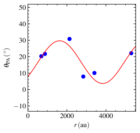
Figure 75: A plot of the radii and position angles of lobes Q4b, Q7, Q8, Q9, K8 and C1, with respect to Q5/K7, for the MYSO G133.7150+01.2155. Least squares fitting of these points is shown in red, which represents a simple precession model.

At C-band we detect emission (left panel of Figure 54) from 7 previously observed lobes (van der Tak et al., 2005) labelled Q1/K2, Q2/K3, Q3/K4, Q4/K6, Q5/K7 (MYSO), Q6/K5 and K8, as well as 5 new lobes labelled, Q4b, Q8, Q9, Q10 and C1 (in accordance with previous naming systems) in the immediate vicinity (within $3\arcsec$) of Q5/K7. At Q-band (right panel of Figure 54) we detect emission coincident with C-band positions for Q2/K3, Q3/K4, Q4, Q5/K7, Q6/K5, Q7 and Q8.

Due to its elongated morphology, jet-like spectral index ($\alpha=0.85\pm 0.07$) and positioning relative to its associated lobes parallel to the SIO-a outflow, Q5/K7 is determined to be a thermal jet with lobes. Shock emission as a result of the jet from Q5/K7 impacting on surrounding material are present in lobes Q4b, Q7, Q8, Q9, K8 and C1. Due to a range in position angle with respect to Q5/K7 we estimate the precession angle, and period, using least squares fitting of a simple, sinusoidal, precession model to the positions (with respect to Q5/K7) for Q4b, Q7, Q8, Q9, K8 and C1 (Figure 75). The inclination and velocity were assumed to be $90\degr$ (i.e. jet is perpendicular to the line of sight) and $500\hbox{${\thinspace\rm{\rm\thinspace km}{\rm\thinspace s}^{-1}\,}$}$ respectively. This resulted in a derived precession period of $43\pm 6{\rm\thinspace yr}$ and precession angle of $37\pm 15\degr$, around an axis oriented at a position angle of $16\pm 5\degr$. Our derived period should be taken as a lower limit if an inclination of the precession axis towards the observer exists. Interestingly the imfit-derived positions for both Q7 and Q8 change from C to Q band, which is likely due to proper motions if both lobes are optically thin shocks as discussed above. Considering that the C and Q-band observations were taken $\sim 2.7{\rm\thinspace yr}$ apart and assuming these to be shock surfaces of the jet (from Q5/K7) upon ambient material, proper motions (in the plane of the sky) are derived to be $303\pm 26\hbox{${\thinspace\rm{\rm\thinspace km}{\rm\thinspace s}^{-1}\,}$}$ at $154\pm 1\degr$ and $353\pm 30\hbox{${\thinspace\rm{\rm\thinspace km}{\rm\thinspace s}^{-1}\,}$}$ at $14\pm 1\degr$ for Q7 and Q8 respectively (adopting a distance of $1.83\pm 0.14{\rm\thinspace kpc}$, Imai et al., 2000), consistent with the derived precession model. These velocity magnitudes are often seen in ionised jets towards MYSOs adding to the case that these changes are proper motion based. It must be conceded that due to the extended nature of these lobes at both C and Q-bands, theses motions may in fact be due to resolving-out effects, however the facts that the two proper motions are equal in magnitude but opposite in direction, the ionized gas is optically thin and that the precession model is consistent with these positional changes adds weight to the proper motion interpretation.

From the spectral index of Q3/K4 ($0.76\pm 0.08$), and the position angle of its major axis at $\theta^{44}_{\mathrm{PA}}=161\pm 15\degr$ which points at the non-thermal lobe Q1/K2, we classify it as a jet with lobes. As for its northern neighbours, Q2/K3 and Q6/K5, we believe one of them to be driving a jet which is powering lobe Q10 due to positional alignment of the C-band emission. From the C-band images, emission appears to be present between Q2/K3 and Q6/K5, which was associated to Q2/K3 by imfit. We therefore believe Q6/K5 to be another jet candidate in the vicinity, while Q2/K3 is classified as a candidate jet with associated lobes, Q10 and the emission between Q2/K3 and Q6/K5. Q4/K6 possesses a steep spectral index ($\alpha=0.93\pm 0.12$) and is coincident with MM6 from Rodón et al. (2008), and we therefore classify it as a jet candidate, due to its ambiguous properties as either a jet or small HCHii region.

With the exception of Q6/K5, all the Q-band sources are within a beam-width ($\sim 0\aas@@fstack{\prime\prime}04$) of their Q-band counterparts from Van der Tak et al. (2005), with a mean separation of $0\aas@@fstack{\prime\prime}026$. Q6/K5 displays a proper motion of $185\pm 7{\rm\thinspace mas}$, or $100\pm 9\hbox{${\thinspace\rm{\rm\thinspace km}{\rm\thinspace s}^{-1}\,}$}$, along a position angle of $-5\pm 2\degr$. However, this latter position comparison is between K and Q-bands. This adds to the complexity of the classification for this source, reinforcing the candidate status of Q6/K5.

Outside the immediate vicinity of G133.7150+01.2155, we also detect two more C-band sources, A and B (the latter of which is also detected at Q), and two sources solely detected at Q-band, QE1 and QE2. These 4 sources have been illustrated separately in Figure 55. Both A and B have near-infrared counterparts in 2MASS imagery, and we determine spectral indices of $-0.56\pm 0.06$ and $-0.13\pm 0.14$ respectively. Considering the imfit derived C-band dimensions of A, this spectral index results from the loss of extended flux at Q-band. Due to its extended nature, we classify it as a UCHii region powered by a B3 ZAMS type star ($\hbox{$\thinspace L_{\rm{bol}}$}=2500\hbox{${\rm\thinspace L_{\odot}}$}$, EM$=(5.5\pm 3.1)\times 10^{6}\rm{\rm\thinspace pc}{\rm\thinspace cm}^{-3}$). Source B remains point-like at all frequencies, and due to its optically thin spectral index and unreddened NIR colour we classify it as a small HCHii region powered by a B3 type ZAMS star ($\hbox{$\thinspace L_{\rm{bol}}$}=2300\hbox{${\rm\thinspace L_{\odot}}$}$, EM$>7.4\times 10^{7}\rm{\rm\thinspace pc}{\rm\thinspace cm}^{-3}$) or later. As for the Q-band only sources, QE1 and QE2, we derived steep, thermal spectral indices of $>2.05\pm 0.05$ and $>1.43\pm 0.07$ respectively. We believe them to be deeply embedded YSOs on account of their non-detection at near-infrared wavelengths and therefore members of the cluster associated to W3 IRS5.

D.2.33 G134.2792+00.8561

In the RGB, 2MASS images of Figure 56, G134.2792+00.8561 is centred on a reddened, elongated (along a position angle of $\sim 110\degr$) source, which itself is spatially confused with a bright, white source. At $11.6{\rm\thinspace\upmu m}$, MICHELLE images show the 2MASS source to break up into 2, possibly 3, sources oriented east to west. Ogura et al. (2002) detect a HH object (HH 586) in images of H$\alpha$ emission at coordinates, $\alpha\,(\mathrm{J2000})=02\hbox{$\rm{}^{h}$}29\hbox{$\rm{}^{m}$}01.1\hbox{$\rm{}^{s}$}$, $\delta\,(\mathrm{J2000})=61\degr 33\arcmin 33\arcsec$ offset from the MYSO’s coordinates by $6.3\arcsec$ at a position angle, $\theta_{\mathrm{PA}}=103\degr$. A bipolar CO molecular outflow is also detected, centred on G134.2792+00.8561, with an outflow position angle and dynamical timescale of $-30\degr$ and $15000{\rm\thinspace yr}$ respectively (Lefloch et al., 1997). Images of continuum-subtracted, $2.122{\rm\thinspace\upmu m}$, H₂ emission, show diffuse, knotted and bipolar morphologies predominantly to the west and south-east of the central source (Navarete et al., 2015).

At the MYSO’s position, we detect a barely resolved source ($167\times 119{\rm\thinspace mas}$ at $\theta_{\mathrm{PA}}=109\pm 63\degr$), labelled as A, with no corresponding detection at Q-band thereby giving an upper limit to its spectral index of $<0.34\pm 0.09$. Due to the alignment of A’s major axis with the Herbig-Haro object, HH 586, it is most likely a thermal jet, however without further information we classify it to be a jet candidate. Approximately $4\arcsec$ to the south of A is an unresolved, $7\sigma$ source at C-band whose established upper limit of $\alpha<0.45\pm 0.11$ fails to constrain it nature. Similarly, the brightest C-band radio source is located $33\arcsec$ south of the MYSO, named C, which has an upper limit to its spectral index of $<-0.12\pm 0.13$. Considering the fact that C does not have a NIR or MIR counterpart, we deduce it to be extragalactic in nature. As for B however, mid-infrared saturation of GLIMPSE images by G134.2792+00.8561 prohibits us from ascertaining its MIR profile and therefore we classify it as unknown in nature. No source was detected over the primary beam in the Q-band image.

D.2.34 G136.3833+02.2666

Relevant previous observations towards this source are limited in the literature, with only millimetric and low-resolution outflow studies being prevalent. Saito et al. (2006) used high resolution mm-studies at $100{\rm\thinspace GHz}$ to resolve three mm-cores within $20\arcsec$ of eachother. The most massive core, core A, is associated to the MYSO, with the other two cores located $15\arcsec$ and $20\arcsec$ to its north east. In the near-infrared, an elongated reflection nebula emanating from the central, reddened source is seen at K-band along an approximate east-west axis. A non-reddened 2MASS source is located $\sim 6\arcsec$ to the west of the MYSO.

At C-band we detect four sources, A, B, C and D, of which only D is not associated to a near-infrared source. Q-band images only detect one source at the same position as the C-band source A, yielding a spectral index of $\alpha=0.92\pm 0.14$. Unfortunately A remains unresolved at both frequencies and without further studies, is classified as a jet candidate. Due to B’s coincidence with a unreddened 2MASS source, and absence of mm-emission (Saito et al., 2006) we classify it to be a partially resolved out Hii region. For both C and D we can not make a definite classification and therefore assign them an unknown status.

D.2.35 G138.2957+01.5552

Also known as AFGL 4029-IRS1, this MYSO’s parental clump harbours a dense cluster of at least 30 B$-$type stars (Deharveng et al., 1997). Remarkably, a previous optical study of this object exists and established velocities of $500\hbox{${\thinspace\rm{\rm\thinspace km}{\rm\thinspace s}^{-1}\,}$}$ for the highly-inclined [Sii] optical jet emanating from this MYSO (Ray et al., 1990). Previous A-configuration, VLA, $3.6{\rm\thinspace cm}$ observations by Zapata et al. (2001) detected a cometary UCHii region (AFGL 4029-IRS2) to the south of G138.2957+01.5552, two compact sources (S and N) separated by $0.6\arcsec$ in the north-south direction (at the MSX source position) and elongated/extended emission along a position angle of $80\degr$ relative to S, which they concluded to be an ionized jet. The radio source N was determined to be a time-variable, low-mass T-Tauri star close to S. A bipolar $2.122{\rm\thinspace\upmu m}$ outflow has previously been detected, comprised of arc-like eastern ($\theta_{PA}=90\degr$) and more compact western emission ($\theta_{PA}=270\degr$), both of which are separated by $\sim 12\arcsec$ ($0.24{\rm\thinspace pc}$) from the MSX source (Navarete et al., 2015).

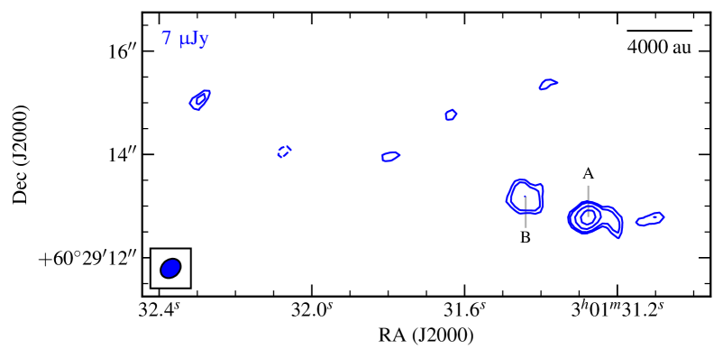
Figure 76: C-band image of G138.2957+01.5552, utilising a robustness of 2 and a restoring beam of $0.421\arcsec\times 0.340\arcsec$ at $-50\degr$. Contour levels are set to $(-3,3,4,7,12,18)\times\sigma$.

Our C-band radio images shown in Figure 58 detect 6 objects within a $1\arcmin$ field of view. Near-infrared, 2MASS, reddened point sources are associated to C, D and E, meaning they are likely YSOs/T-tauri stars which are members of the cluster established by Deharveng et al. (1997). A resolved out Hii region is detected, associated to a bright 2MASS source, which is the previously detected cometary UCHii region. Source A is centred at the pointing centre and is the only radio object also detected in our Q-band images. It is separated from B, which lies at a position angle of $72\degr$ relative to A, by $1.3\arcsec$. Considering the alignment with the established outflow axis we determine B (which appears partially resolved out) to be a lobe of shock emission, especially given its lack of an infrared counterpart. Being located at the MYSO’s position and with its spectral index typical of an ionized jet of $0.69\pm 0.11$, A is classified as a thermal jet with lobes. In our images however, we detect no emission from the position of source N from Zapata et al. (2001), which is not due to resolving out effects (our beam is practically identical to theirs) or sensitivity issues (image RMS noise is $\sim 2$ times lower). We believe that the previously established time-variability is the reason for our non-detection of N.

Considering the absence of previously detected emission (N) and apparent resolving out effects towards A2, the C-band data was re-imaged with a robustness of 2, the results of which are shown in Figure 76. The new, more sensitive robustness shows how B was indeed resolved out in the images of Figure 58, but also that significant ($>5\sigma$), arc-like emission is also detected at a position angle of $-100\degr$ from A with an imfit derived flux of $128\pm 21{\rm\thinspace\upmu Jy}$. With this measurement, the flux of A decreases to $71\pm 10{\rm\thinspace\upmu Jy}$, giving a spectral index of $\alpha=1.0\pm 0.1$. For consistency however, we use the value for flux and spectral index from the clean maps with a robustness of $0.5$ in the analysis within the main body of this work. A $4\sigma$ component is also detected $4\arcsec$ to the ENE of A, in line with the jet’s outflow axis which, if real, is likely to be another shock surface interacting with the jet.

D.2.36 G139.9091+00.1969A

Associated to the cluster AFGL437 of at least 60 members, this is a well studied object. At the centre of the cluster, three near-infrared sources dominate in terms of flux with both diffuse, knotted and bipolar 2.122${\rm\thinspace\upmu m}$, H₂ emission detected at a variety of position angles (Navarete et al., 2015) with respect to the MYSO. A relatively uncollimated, CO, molecular outflow was detected oriented roughly on a north (red) - south (blue) axis (Gomez et al., 1992), whose material was hypothesised to be sourced from laminar flow of dragged gas from outflow cavity walls. Weintraub & Kastner (1996) resolved the northern-most of the three NIR sources into two, dubbed WK34 and WK35, of which WK34 was determined to be a low-luminosity protostar driving the north-south molecular outflow and located at the centre of a similarly oriented reflection nebula (Meakin et al., 2005). From those works, the other NIR sources were dubbed S (our target) and W for the southern and western bright NIR sources respectively. NIR speckle imagery by Alvarez et al. (2004) showed a monopolar reflection nebula centred on S and extended towards the SE ($\theta_{\rm PA}=135\pm 10\degr$), which highlights the position of an outflow cavity.

We detect three C-band sources, all of which are associated with near-infrared objects in 2MASS imagery and only one of which (the Hii region) is not detected at Q-band. The radio object A (the southern-most NIR source, S, from Weintraub & Kastner, 1996) is extended at a position angle of $62\degr$ in the direction of Ab, which is located $0.3\arcsec$ from A at a position angle of $58\degr$. To the south-west of A is the low-SNR source, Ac, separated by $0.7\arcsec$ (at $\theta_{PA}=241\degr$). Calculated values of $\alpha$ and $\gamma$, for A, are $0.42\pm 0.08$ and $-0.81\pm 0.19$ respectively, which agree well with the models of Reynolds (1986). However, due to the extended emission being perpendicular to the defined outflow cavities, we believe this source is a photo-evaporative disc wind. The discrepancy from the expected value of $\alpha\sim 0.6$ is likely due to resolving out effects moving from C to Q-bands. At Q-band the source seems roughly quadrupolar, and in light of the disc wind classification, is likely tracing the NE portion of the wind.

Approximately $9\arcsec$ north-west of A is a spherical Hii region (the NIR source, W), with a C-band flux of $20.5\pm 1.2{\rm\thinspace mJy}$ which is therefore (assuming it is optically thin at C-band) powered by a B1 type star with a bolometric luminosity of $11000\hbox{${\rm\thinspace L_{\odot}}$}$ (Davies et al., 2011). This agrees well with the $10000\hbox{${\rm\thinspace L_{\odot}}$}$ (Lumsden et al., 2013) calculated from the infrared SED of its alias in the RMS survey.

Located $10\arcsec$ north of A is the weakest C/Q-band source, B (also known as WK34), which is unresolved at both frequencies. Derived to have a spectral index of $\alpha=1.13\pm 0.16$, it is classified as a nearby YSO, which may be powering a small HCHii region, or an ionized jet.

D.2.37 G141.9996+01.8202

Near and mid-infrared surveys show a bright source which saturates in 2MASS, UKIDSS and GLIMPSE images. Mitchell et al. (1992) observed a CO $J=2\rightarrow 1$ outflow, with G141.9996+01.8202 (alias AFGL490) at the centre of the red and blue lobes. The molecular outflow’s red lobe peaked $\sim 20\arcsec$ to the north-west but extended in an arc round to the north east of AFGL490, with the blue lobe situated at a position angle of $225\degr$ (i.e. anti-parallel to the arc of red emission). A cold envelope elongated at a position angle of $\sim-45\degr$ was observed in the sub-mm continuum, while simultaneous observations of CS $J=2\rightarrow 1$ showed evidence for multiple outflows driven by low-mass sources in the envelope (Schreyer et al., 2002). Further PdBI observations of C¹⁷O $(2-1)$ revealed a rotating, clumpy, molecular disc with an inclination of $35\degr$ and major axis oriented at a position angle of $105\degr$ (Schreyer et al., 2006).

In our C-band images, we detect 3 compact sources labelled A (the MYSO), B and C, all of which are coincident with a NIR source. Only A was detected at Q-band, the images of which show an interesting morphology with a compact radio ‘core’ embedded in (partially) resolved-out emission. Initially it was thought that the extended component was the dominant emission detected at C-band, however A’s C-band dimensions ($0.21\arcsec\times 0.06\arcsec$ at $58\degr$) do not coincide with the patches of extended emission at Q-band. Values derived for $\alpha$ and $\gamma$ closely agree to those of a spherical, stellar wind (Panagia & Felli, 1975), thermal jet or disc wind, all of which are supported by the presence of the shock tracer [FeII] at $1.64{\rm\thinspace\upmu m}$ in NIR spectra (Cooper et al., 2013). Since the derived position angle of the C-band component is as equally aligned with the inferred disc’s major axis, as it is with the molecular outflow, we classify this as a jet candidate. As a further note, considering its relatively evolved status in the literature (in comparison to this sample), it is likely that the stellar wind (especially given IR recombination line profiles seen by Bunn et al., 1995), or photo-evaporative disc wind picture is correct, however more observations are required to distinguish between all three possibilities. As for the nature of the extended emission, under the assumption that the central object has evolved past the MYSO stage and is beginning to produce appreciable Lyman fluxes, it could be sources from ionized cavity walls, disc surfaces or an optically thick Hii region. Both B and C are almost certainly members of the same cluster, however their classification, although almost certainly not extragalactic, is unknown.

D.2.38 G143.8118$-$01.5699

Near-infrared images show a reddened source at the MYSO position which is embedded in a cluster $1.8\arcmin\times 1.4\arcmin$ in size (Bica et al., 2003). Navarete et al. (2015) detect no emission in $2.122{\rm\thinspace\upmu m}$ H₂ towards this object.

Although we do not detect anything at $44{\rm\thinspace GHz}$, we see three, low-flux, compact sources in C-band images, A (G143.8118$-$01.5699), B and C, of which all have near-infrared counterparts. Although A and B are resolved according to imfit routines, their signal to noise is low and consequently the errors on deconvolved position angles/dimensions are large. Considering the relatively unconstrained nature of the emission detected towards all C-band sources, we therefore classify A to be a jet candidate, while B and C, although certainly no extragalactic, are of unknown classification.

D.2.39 G148.1201+00.2928

Another object with a small observation history, the most relevant of which were the H₂, $2.122{\rm\thinspace\upmu m}$ observations by Navarete et al. (2015) which detected diffuse, knotted and bipolar, shock emission at position angles of $160-215\degr$ and separations between $0.27$ and $1.08{\rm\thinspace pc}$. In 2MASS images, the MYSO is situated in a cluster, with a diffuse reflection nebula emanating from it towards the north-west ($\theta_{\mathrm{PA}}\sim 110\degr$).

At $5.8{\rm\thinspace GHz}$, we detect three sources within the inner $60\arcsec$ of the field of view. One of these sources (A) is coincident with the MYSO from the RMS survey, while the other two are coincident with other NIR objects in the field. The C-band radio source A breaks up into two Q-band sources whose peaks are separated by $0.1\arcsec$ ($320{\rm\thinspace au}$), with the weaker lobe (A2) located at a position angle of $295\degr$ from the other (A), roughly aligned with the NIR reflection nebula. Because both Q-band sources (A and A2) are coincident with the C-band image of A, we combine the Q-band fluxes of A and A2 and find a spectral index of $\alpha=1.13\pm 0.14$ for the MYSO. From this information, A and A2 may be a jet/counter-jet system, or a close binary system. If a jet/counterjet, from the models of Reynolds (1986) the derived spectral index would suggest some degree of recombination or acceleration in the flow which, if the separation represents the collimation radius (i.e. where the toroidal become dominant over the poloidal component in the launching magnetic field), would be more likely from acceleration. A piece of evidence against the biconical jet scenario would be the position angles of shocked H₂ emission observed by Navarete et al. (2015), which are misaligned with the apparent jet’s axis. Due to these considerations, we define A/A2 to be a jet candidate. As for B and C, upper limits on the spectral indices of $<0.63\pm 0.12$ and $<-0.01\pm 0.05$ do not constrain their natures much and therefore, although not extragalactic, are assigned the unknown classification.

D.2.40 G160.1452+03.1559

Near-infrared UKIDSS images (colourscale in Figure 63 respectively) show that the reddened MYSO is extended in the NIR (especially UFTI imagery), highlighting the possibility of cavities at a position angle of $\sim 100\degr$, an interpretation backed up by the detection of a parallel ¹²CO $(2-1)$ outflow by Xu et al. (2012). Radio observations by Sánchez-Monge et al. (2008) detect a compact radio source centred on the MYSO at $3.6{\rm\thinspace cm}$, $1.3{\rm\thinspace cm}$, $7{\rm\thinspace mm}$ and $1.2{\rm\thinspace mm}$ (IRAM) with a spectral index between $3.6{\rm\thinspace cm}$ and $1.3{\rm\thinspace cm}$ of $\alpha=1.1\pm 0.4$. Targeted, near-infrared observations showed a H₂, $2.122{\rm\thinspace\upmu m}$, collimated outflow parallel to both the molecular outflow’s, and radio source’s major, axes at a position angle of $126\degr$ which extended over a length of $>0.35{\rm\thinspace pc}$ (Varricatt et al., 2010).

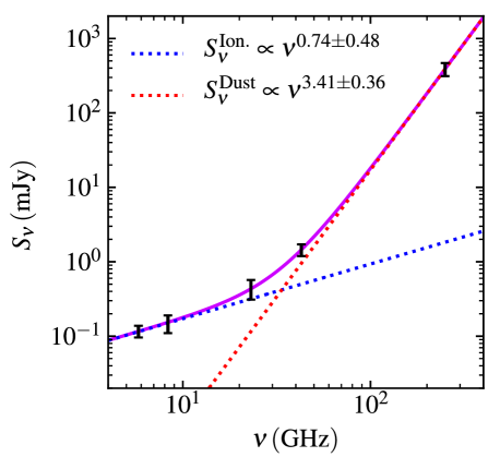
Figure 77: Plot of flux against frequency for source ‘A’ of G160.1452+03.1559, utilising data at $8{\rm\thinspace GHz}$, $23{\rm\thinspace GHz}$, $43{\rm\thinspace GHz}$ and $250{\rm\thinspace GHz}$ from Sánchez-Monge et al. (2008). The least squares fit is plotted as the purple line for a double power law, with each power law component plotted as a dotted red (dust) and blue (ionized) line. Derived power laws for the dust and ionized contributions are indicated in the top left corner.

This source was only observed at C-band, the images of which show two compact sources in the field of view, one situated on the MYSO (A) and the other (B) offset $\sim 3\arcsec$ to the SSE. Although B was too low in terms of signal to noise for its dimensions to be derived by imfit, A has a major axis aligned along a position angle of $\sim 110\degr$, parallel with the apparent outflow cavities seen in NIR images. In order to try to discern A’s nature, the data from Sánchez-Monge et al. (2008) was combined with our C-band result and fitted with a power law consisting of a dust and an ionized component (assuming no flux variability between the two datasets). The resulting fit has been plotted in Figure 77, deriving a spectral index for the ionized component of $\alpha=0.74\pm 0.48$, expected of a typical ionized jet. Using the derived power law we calculate a flux contribution from the ionized component, at $43{\rm\thinspace GHz}$, of $500{\rm\thinspace\upmu Jy}$ which is equivalent to an optically thin Hii region powered by a ZAMS type B3 star with a luminosity of $\sim 2500\pm 2000\hbox{${\rm\thinspace L_{\odot}}$}$. Comparing this to the IR derived flux of $2100\hbox{${\rm\thinspace L_{\odot}}$}$, it appears that the radio flux is also compatible with a HCHii region with an average electron density of $8\pm 7\times 10^{4}{\rm\thinspace cm}^{-3}$. However, because of its extensive observational history, with collimated, H₂, shock features, molecular outflows and a full sampling of its radio spectrum, the ionized jet scenario is extremely likely. We therefore have classified A as an ionized jet. Component B, being associated with a reddened near-infrared source is likely a coeval low-mass YSO, however more observations are needed to clarify this.

D.2.41 G173.4839+02.4317

Our field of view contains two MYSOs from the RMS database, G173.4839+02.4317 and G173.4815+02.4459. In 2MASS images (middle panel of Figure 64), G173.4839+02.4317 displays as a relatively unreddened, bright source surrounded by a small, young cluster (Ginsburg et al., 2009), while the reddened, near-infrared source, G173.4815+02.4459 shows significant, EGO emission at $4.5{\rm\thinspace\upmu m}$ (see GLIMPSE inset of Figure 64) whose diffusivity extends along a rough north-west to south-east axis. The EGO emission is embedded in a protocluster according to Ginsburg et al. (2009) who also inferred that G173.4815+02.4459 was, in fact, a massive binary system with a separation of $400{\rm\thinspace au}$. H₂, $2.122{\rm\thinspace\upmu m}$ observations show an outflow at a position angle of $\sim 150\degr$ centred on G173.4839+02.4317 (components 7/8 and 1a/b/c from Varricatt et al., 2010; Navarete et al., 2015, respectively). Most other observations concentrate on G173.4815+02.4459, for example Beuther et al. (2002b) detect 3 condensations in H¹³CO⁺ $(1-0)$, condensation ‘1’ being centred on G173.4815+02.4459, and condensations ‘2’ and ‘3’ located $16\arcsec$ and $25\arcsec$ to the west of condensation ‘1’ respectively. A highly collimated outflow in CO $(1-0)$, at a position angle of $\sim 165\degr$, which terminates in H₂ bow-shocks, is detected centred on condensation ‘1’ which is also at the centre of a high-velocity CO $(1-0)$ outflow at a position angle of $\sim 130\degr$, parallel to the EGO’s diffuse emission. Core ‘2’ powers an SiO $(2-1)$ outflow at a position angle of $\sim 15\degr$. Simultaneous $2.6{\rm\thinspace mm}$ observations showed condensation ‘1’ to break into 3 mm-cores, with the brightest core, mm1, being centred on the MYSO and the other two mm-cores, mm2 and mm3, positioned $4\arcsec$ to the east and $8\arcsec$ to the north-west of mm1 respectively. Further sub-mm observations (Beuther et al., 2007) resolved mm1 into two further sub-cores (one of which was detected by the VLA at X-band), and mm2 into 4 further sub-cores, creating a complicated picture of this particular massive star-forming site. From the spectral energy distribution across cm, mm and sub-mm wavelengths, mm2 was also hypothesised to be emission from an outflow/jet. At other wavelengths, both the collimated, and high-velocity, molecular outflows are also seen in line emission in the near-infrared (Varricatt et al., 2010; Navarete et al., 2015). Perpendicular to the established H₂, and high-velocity molecular, outflows, a line of CH₃OH masers ($\theta_{\mathrm{PA}}\sim 35\degr$), along a velocity gradient suggestive of Keplerian rotation in an accretion disc, were detected by VLBI observations (taken in 1997, Minier et al., 2000).

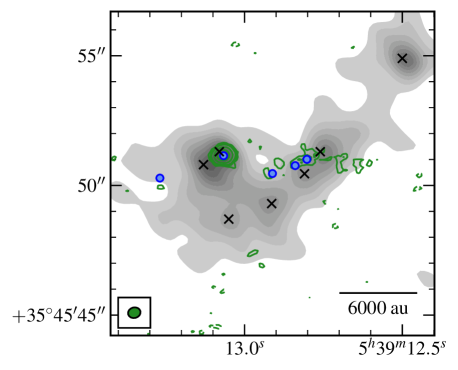
Figure 78: Sub-mm continuum image of G173.4815+02.4459 at $1.2{\rm\thinspace mm}$ (PdBI, greyscale) with $8.4{\rm\thinspace GHz}$ VLA data overlayed (green contours). The ‘x’ markers show the position of the 5 cores from Beuther et al. (2007) and the blue ‘$\circ$’ markers show the positions of the 5 sources, E1, E2, E3, E4 and E5, that we detected at C-band. Grey-scale increases by $10\%$ from $10\%$ to $90\%$ of the peak flux ($58.9{\rm\thinspace mJy}\,\mathrm{beam}^{-1}$), while green contours are set at $-3,3,4,5,10$ and $20\sigma$ ($\sigma=16.4{\rm\thinspace\upmu Jy}\,\mathrm{beam}^{-1}$). Both the $8.4{\rm\thinspace GHz}$ VLA and $1.2{\rm\thinspace mm}$ PdBI data are from Beuther et al. (2007).

Within $1\arcmin$ of the two MYSOs in our field of view, we detect a total of 12 different C-band radio sources. Component E1$\rightarrow$E5 are associated with G173.4815+02.4459, while A1 and A2 are associated to G173.4839+02.4317. Components B, C, D, E and F are not associated to any infrared source, while G is coincident with a bright, unreddened 2MASS source. We detect a methanol maser located at E1’s position which is coincident with the EGO from GLIMPSE images (top left panel in Figure 64). High-resolution NIR images show that E2, E3, E4 and E5 are not associated with any near-infrared point sources, only diffuse emission (Figure 1c of Yan et al., 2010). Those same NIR images were however saturated around our component A1 and therefore we are unable to discern if A2 has its own infrared source. In order to better understand the natures of E1$\rightarrow$E5, we plotted their positions on top of previous mm and radio observations in Figure 78 from Beuther et al. (2007). E1 is located at the position of core mm1a from Beuther et al. (2007) and is also detected at X-band (we calculate $\alpha=1.5\pm 0.4$ between C and X-band), while E2 and E5 are not co-located with any $1.2{\rm\thinspace mm}$ emission. There is also diffuse, low-SNR, X-band emission coincident with E2, E3 and E4 with a rough spectral index of $\sim 0$. E3 and E4 are located towards the mm-core, mm2b, which was the core with an inferred emission contribution from a jet/outflow. Considering the wealth of previous observations, it is clear that E1 is driving a collimated, outflow and therefore harbours an ionized jet with associated lobes. We believe that E5 is a lobe as a result of jet-shocks on surrounding material, considering its position angle from the MYSO (along which there is another $3\sigma$ lobe $\sim 1.1\arcsec$ ESE of E5). As for E2, E3 and E4, there is a variety in position angle offsets from E1. If the massive binary scenario from Ginsburg et al. (2009) is accurate, large precessional shifts may be affecting the north-western side of the jet, providing a mechanism to alter the jet’s outflow axis and we tentatively classify E2, E3 and E4 as shock-excited lobes on this basis. Interestingly our source F is also located along a similar axis from E1 as E5 and therefore may be another lobe, however this is uncertain. Sources A2, B, C and D are not easy to classify considering their absence of previous detections and are therefore of unknown classification. From its near-infrared profile and evolved status in the literature, G173.4839+02.4317 is almost certainly a Hii region, especially considering both its strong Br$\gamma$ emission in the near-infrared (Cooper et al., 2013) and C-band, radio-inferred bolometric luminosity of $2450\hbox{${\rm\thinspace L_{\odot}}$}$ which agrees with that derived from IR studies ($2900\hbox{${\rm\thinspace L_{\odot}}$}$). As for G, due to its bright, main sequence near-infrared profile, it is likely to be a main-sequence star.

D.2.42 G174.1974$-$00.0763

Located in an active star formation region with a rich observational history, the MSX source G174.1974$-$00.0763 is a relatively unreddened, bright near-infrared 2MASS source, with a saturated mid-infrared profile surrounded by diffuse $8{\rm\thinspace\upmu m}$ PAH emission, typical of Hii regions. Carral et al. (1999) detect a faint radio source at $8.4{\rm\thinspace GHz}$ with a flux of $0.30\pm 0.06{\rm\thinspace mJy}$. Within $60\arcsec$ of the pointing centre is another MYSO, at an earlier stage in evolution, referred to in the literature as AFGL 5142 ($\alpha\,(\mathrm{J2000})=05\hbox{$\rm{}^{h}$}30\hbox{$\rm{}^{m}$}48.02\hbox{$\rm{}^{s}$},\delta\,(\mathrm{J2000})=33\degr 47\arcmin 54.5\arcsec$). In GLIMPSE images, it is at the heart of a dense cluster, while at near-infrared, dust extinction gives it a faint, reddened profile in 2MASS images. AFGL 5142 is listed as possessing a bolometric luminosity of $2300\hbox{${\rm\thinspace L_{\odot}}$}$ (Palau et al., 2011), which is revised to $3300\hbox{${\rm\thinspace L_{\odot}}$}$ in light of the more accurate distance estimate of $2.14^{+0.051}_{-0.049}{\rm\thinspace kpc}$ by Burns et al. (2017). AFGL 5142 is positioned at the centre of collimated HCO⁺ $(1-0)$ and SiO$(\mathrm{v}=0,2-1)$ outflows, along a position angle of $\sim 5\degr$ (Hunter et al., 1999), as well as co-located with a compact radio source ($0.83\pm 0.15{\rm\thinspace mJy}$ at $8.4{\rm\thinspace GHz}$ using the VLA in A-configuration, Hunter et al., 1995). However, it appears this source may be prone to resolving out effects and/or variability at radio wavelengths (see Figure 2 of Goddi & Moscadelli (2006) for a summary), for example a higher flux of $1{\rm\thinspace mJy}$ was reported by Carpenter et al. (1990) for D-configuration $4.86{\rm\thinspace GHz}$ observations (performed 1989), and $1.5\pm 0.3{\rm\thinspace mJy}$ reported by Hunter et al. (1995) at $8.6{\rm\thinspace GHz}$ which used B-configuration observations (taken 1998). Later studies at $8.4{\rm\thinspace GHz}$ show that the continuum source breaks down in to 2 separate sources named, CM-1A and CM-1B, and also appears to power a further two molecular outflows at position angles of $35\degr$ and $-60\degr$ (Zhang et al., 2007). PdBI, $1.3{\rm\thinspace mm}$ observations by Palau et al. (2011) showed that two mm-cores were located with the MYSO. Of these, MM1 is attributed to the previous radio detections of the literature, and is elongated at a position angle of $94\degr$ (perpendicular to the north-south outflow), whereas MM2 is situated $\sim 1\arcsec$ to its south and may have been previously detected at $8.4{\rm\thinspace GHz}$ (with a peak flux of $0.35\pm 0.09{\rm\thinspace mJy},$ Zhang et al., 2007).

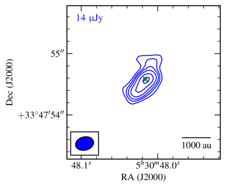
Figure 79: Re-imaged C-band data of source B (AFGL 5172) from the G174.1974$-$00.0763 field, utilising a robustness of -1. Contours are set at $-3,3,5,7,10,15$ and $20\sigma$ where $\sigma=14.1{\rm\thinspace\upmu Jy}\,\mathrm{beam}^{-1}$. The restoring beam’s dimensions were $0.299\arcsec\times 0.218\arcsec$ at $\theta_{\mathrm{PA}}=104\degr$.

From the C-band data, we report the detection of 3 radio sources, A, B and C, of which A is located at the same position as G174.1974$-$00.0763, and both B and C are colocated with near-infared/mid-infrared sources, $24\arcsec$ to the east and $51\arcsec$ to the WNW respectively. Using the radio flux at $8.4{\rm\thinspace GHz}$ of $0.30\pm 0.06{\rm\thinspace mJy}$ from Carral et al. (1999), we calculate a spectral index for A of $\alpha=2.3\pm 0.7$, typical of optically thick emission from a Hii region. It must be conceded that the flux from the literature used observations from 1994 with the VLA in its most compact configuration, therefore the resolving out of flux and/or variability may affect this calculated value. However, considering its near and mid-infrared appearance, likely optically thick radio spectrum and diffuse $8{\rm\thinspace\upmu m}$ emission, it is determined that A is a HCHii region. As for B, in combination with our C-band flux of $726\pm 22{\rm\thinspace\upmu Jy}$, we calculate a spectral index for B of $0.4\pm 0.5$. However, as previously discussed, this derived spectral index is not very useful in trying to establish whether or not the emission stems from an ionized jet on account of resolving out/variability issues apparent in the literature. Since Zhang et al. (2007) resolve B into two sources, we reimaged the field using a robustness of -1, in order to increase the effective resolution. The results are plotted in Figure 79 which more reliably shows two components, one elongated at a position angle of $\sim 0\degr$ from the peak emission, and the other elongated at a position angle of $\sim-50\degr$. Zhang et al. (2007) recorded almost equal fluxes at $8.4{\rm\thinspace GHz}$ for both of these sources, whereas our $5.8{\rm\thinspace GHz}$ data shows the most southern to be the strongest. This may be due to spectral index effects, or variability, however further observations are required to clarify this. It is believed however that the northern elongation is an ionized jet driving the well establish north-south outflows and we therefore classify B to be an ionized jet. Our detected source C has no previous detections present in the literature, however considering its coincidence with a bright main-sequence star in the near-infrared, it is likely a stellar wind, however more radio observations will be required to determine this.

D.2.43 G177.7291$-$00.3358

K-band, near-infrared, continuum images show a bright point source at the centre of a quadrupolar patch of extended emission with a UIB feature indicative of UV excitation (see Figure 1y of Ishii et al., 2002, who associated the morphology to tracing cavity walls). Low-resolution, near-infrared spectra taken with a slit alignment of $\theta_{\mathrm{PA}}=-70\degr$ (i.e. along the NW-SE, K-band diffusivity) shows shocked, [$\mathrm{FeII}$] emission, a weak Br$\gamma$ line and CO ($v=2-0$) bandhead emission (Cooper et al., 2013), presumably from an accretion disc (Ilee et al., 2013). Non-detection of both methanol (where $3\sigma=150{\rm\thinspace mJy}$), and water, masers towards this source has been recorded by Fontani et al. (2010).

Two C-band sources are detected in the inner $60\arcsec$ of our field of view, labelled A (the MYSO) and B (located $25\arcsec$ west of A). Component A is completely unresolved at C-band, whereas B has dimensions of $0.16\arcsec\times 0.13\arcsec$ with large errors on account of low signal to noise and barely extended structure. Assuming an optically thin Hii region, from the C-band flux for A we infer a bolometric luminosity of $1300\hbox{${\rm\thinspace L_{\odot}}$}$ (Davies et al., 2011), close to that derived from the infrared ($2300\hbox{${\rm\thinspace L_{\odot}}$}$), especially considering the radio emission is likely still partially optically thick. Therefore neither jet, nor compact Hii, gains precedence and therefore we classify A as a jet candidate. As for B, it is aligned with the outflow cavities’ central axis seen at near-infrared wavelengths yet lacks an (mid or near) infrared counterpart, and therefore could be a shocked, Herbig-Haro type object (especially given its resolved dimensions) from a jet. However without more spectral information we must determine it to be of an unknown nature due to its similarity to extragalactic phenomena.

D.2.44 G183.3485$-$00.5751

Near-infrared, K-band images show diffuse emission elongated along a NW-SE axis, with the MYSO’s reddened source at its centre. From C¹⁸O observations, a clump $0.76{\rm\thinspace pc}$ ($75\arcsec$) in diameter was detected with a mass of $250\hbox{${\rm\thinspace M_{\odot}}$}$ (Wu et al., 2011), whose peak is offset to the MYSO’s position by $14\arcsec$ to the south-west. No other relevant observations are present in the literature.

Our observations detect two, point-like, C-band sources, one (A) is roughly positioned at the MYSO’s location, while the second (B) is co-located with a main sequence (from its near-infrared colours) star. We also detect two methanol maser spots separated from A’s location by $0.22\arcsec$ and $0.32\arcsec$, at position angles of $189\degr$ and $341\degr$ respectively. The positioning of the methanol masers, along the edges of the diffuse emission, would suggest them to reside in the cavity walls, rather than in the disc (which would need to be at least $1000{\rm\thinspace au}$ in diameter). From the sparsity of information on this source, it is impossible to definitively classify A and we assign it candidacy as a jet. Source B’s positioning with a main sequence star means it is likely a stellar wind, though further radio data, at a variety of frequencies, are needed to clarify this.

D.2.45 G188.9479+00.8871

Located in the star formation region AFGL 5180, G188.9479+00.8871 is commonly referred to as NIRS1 (following the work of Tamura et al., 1991, who identified 11 K-band point sources in its proximity) and has an established, bipolar, CO outflow at a P.A. of $\sim 130\degr$ detected by Snell et al. (1988). The RMS source is at the centre of a bipolar, $2.122{\rm\thinspace\upmu m}$, H₂ outflow at a position angle of $110\degr$ (1a/1b from Navarete et al., 2015) as well as two diffuse, bipolar, K-band, reflection nebula at position angles of $90\degr$ and $110\degr$ (Tamura et al., 1991). Saito et al. (2006) detect 11 cores in C${}^{1}8$O, with core F associated to NIRS1, and two continuum sources at $98{\rm\thinspace GHz}$, of which core F is coincident with one (MCS B) and core E with the other (MCS A, the brightest), which in turn is located with the NIR source, NIRS5. Both of the continuum sources were previously detected as $1.2{\rm\thinspace mm}$ cores by Minier et al. (2005), with bolometric luminosities of $7.0\times 10^{3}\hbox{${\rm\thinspace L_{\odot}}$}$ and $2.4\times 10^{4}\hbox{${\rm\thinspace L_{\odot}}$}$ for NIRS1 and NIRS5 respectively (reduced following the more accurate distance estimate of $1.76\pm 0.11{\rm\thinspace kpc}$ by Oh et al., 2010). VLBI observations of CH₃OH masers show a linear arrangement of maser spots along a position angle of $78\pm 7\degr$, with an inferred magnetic field direction parallel to the CO outflow (Surcis et al., 2013).

At C-band we detect 5 distinct radio sources. Sources A and B1/B2 are unresolved and coincident with the C¹⁸O cores F and E, from Saito et al. (2006), respectively, while C and D are resolved and have no mm-counterparts in the literature but are associated to near-infrared sources. A methanol maser is also detected to be coincident with continuum source A. Considering the wide variety of outflow phenomena seen, we believe A to be a jet, however without more information at a range of frequencies we can only classify it as a candidate. As for B1 and B2, interestingly the axis running through them in a direction parallel to extended 98${\rm\thinspace GHz}$ emission from Saito et al. (2006), which may include contribution from an ionised jet assuming B1/B2 are a jet/lobe pair. As with A, more information is required, and consequently B1 is determined to be a candidate jet with lobes (B2). Component C’s coincidence with a near-infrared source classifies it as a cluster member, but the origin of its radio emission is unclear. Due to its extended nature, presence of resolved out emission and mid-infrared appearance in GLIMPSE images, we classify D to be a Hii region.

D.2.46 G189.0307+00.7821

Also known as AFGL 6366S, this source is located with a K-band, reflection nebula, indicative of outflow cavities, along a rough north-west to south-east axis. Approximately $100\arcsec$ to the ENE another YSO, G189.0323+00.8092 (alias AFGL 6366N) from the RMS database ($\hbox{$\thinspace L_{\rm{bol}}$}=1.1\times 10^{4}\hbox{${\rm\thinspace L_{\odot}}$}$), is within our C-band field of view and is another YSO which has diffuse NIR emission towards its east. Kurtz et al. (1994) detect a $0.6\pm 0.06{\rm\thinspace mJy}$, unresolved, $8.4{\rm\thinspace GHz}$ source at $\alpha\,(\mathrm{J2000})=06\hbox{$\rm{}^{h}$}08\hbox{$\rm{}^{m}$}40.66\hbox{$\rm{}^{s}$},\delta\,(\mathrm{J2000})=21\degr 31\arcmin 07.3\arcsec$ (slightly offset to G189.0307+00.7821’s position), with an unlisted $\sim 0.25{\rm\thinspace mJy}$ source $\sim 2\arcsec$ south west of it. Observations at 98 and 110${\rm\thinspace GHz}$ show that there are two mm-cores (also detected in C¹⁸O), one centred on G189.0307+00.7821’s coordinates (MCS A) and the other (MCS B) located approximately $8\arcsec$ to it north-east (Saito et al., 2008). Two molecular clumps, one coincident with G189.0307+00.7821 (clump 3a) and the other located $\sim 140\arcsec$ to its ENE (clump 3b, positioned with G189.0323+00.8092) were detected in single dish ¹³CO ($J=1-0$) observations by Shimoikura et al. (2013). Along a position angle of $\sim 100\degr$, Wu et al. (2010) detected a bipolar, ¹²CO ($1-0$) outflow, centred on G189.0307+00.7821, with the blue lobe towards the west, along the same position angle that Navarete et al. (2015) detect a knot of H₂ emission, as well as a bipolar H₂ outflow at a position angle of $\sim 130\degr$.

Within $60\arcsec$ of the pointing centre we detect 7 radio sources in our C-band image. Four of these are located within $8\arcsec$ of the reddened 2MASS source shown in the top left panel of Figure 69, named A1, A2, B and C, the last of which we also detect a methanol maser towards. Comparing to NIR, UIST images, A1 is associated to the bright K-band source, while A2, B and C do not have a NIR counterpart. In $12{\rm\thinspace\upmu m}$ MICHELLE images however, it can be seen that both A1 and C have mid-infrared counterparts, suggesting that C’s YSO is more deeply embedded in the natal clump (clump 3a from Shimoikura et al., 2013). It is also relevant to note that component C was previously detected by Kurtz et al. (1994) (see above) and, assuming no variability, therefore has a spectral index of $\alpha=0.4\pm 0.4$ between $5.8$ and $8.4{\rm\thinspace GHz}$. As for the natures of these central components, given the CO ($\theta_{\mathrm{PA}}\sim 100\degr$) and H₂ outflows centred on A1, a strong case could be made for A2 being a shocked lobe along the jets path. We therefore (through lack of more radio information), classify A1 to be a candidate jet with lobes. Due to C’s coincidence with both a methanol maser and mid-infrared source, it is almost certainly another MYSO in the vicinity of G189.0307+00.7821, however the nature of its radio emission is unconstrained. Due to C’s deconvolved dimensions, the major axis of which is aligned along a position angle parallel to the axis through B and C, B may be a shocked lobe of emission related to a jet at C. However more information is again needed and we therefore designate C as a candidate jet with lobes. As for the other three sources, both D and F have no near, or mid, infrared counterparts and are located away from the clump’s sub-mm emission, but are aligned along the same position angle as A2, relative to A1. Therefore it is quite possible that these are also lobes of shocked emission significantly more separated from the jet’s launching site than A2. However, considering the speculative nature of this and that a serendipitous alignment of background sources is a possibility, we therefore classify them as unknown sources. Due to its clear near-infrared profile as a blue, main-sequence star, we classify E as a likely stellar wind.

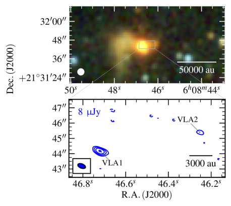
Figure 80: Near-infrared (top panel; 2MASS, $\mathrm{K,H,J}$ R, G, B colour-scale) and C-band radio map (bottom) of G189.0323+00.8092. Restoring beams are the same as in Figure 69, while contour levels are set at $(-3,3,6,11,21)\times\sigma$.

As previously mentioned, another MYSO (G189.0323+00.8092) is registered in the RMS database $100\arcsec$ to the ENE of G189.0307+00.7821, and coincident with another molecular clump. Inspection of the C-band data outside the central $1\arcmin$, shows a radio source coincident with the second YSO’s position (VLA1) and a $6\sigma$ source $\sim 7\arcsec$ to its east (VLA2). In Figure 80 these sources are presented in conjunction with a 2MASS, NIR image. Using imfit, we derive VLA1’s right ascension to be $06\hbox{$\rm{}^{h}$}08\hbox{$\rm{}^{m}$}46.7192\hbox{$\rm{}^{s}$}\pm 0.014\arcsec$, declination to be $+21\degr 31\arcmin 44.164\arcsec\pm 0.007\arcsec$, with a flux of $212\pm 16{\rm\thinspace\upmu Jy}$ and dimensions $(287\pm 84{\rm\thinspace mas})\times(76\pm 67{\rm\thinspace mas})$ at $\theta_{\mathrm{PA}}=69\pm 13\degr$. Those same properties derived for the unresolved source VLA2 are $\alpha\,(\mathrm{J2000})=06\hbox{$\rm{}^{h}$}08\hbox{$\rm{}^{m}$}46.2528\hbox{$\rm{}^{s}$}\pm 0.054\arcsec$, $\delta\,(\mathrm{J2000})=+21\degr 31\arcmin 45.383\arcsec\pm 0.015\arcsec$ and a flux of $43\pm 13{\rm\thinspace\upmu Jy}$. For VLA1, the radio flux is equivalent to an optically thin Hii region powered by a central object with a bolometric luminosity of $1700\hbox{${\rm\thinspace L_{\odot}}$}$. Considering the emission is likely still optically thick, this under-luminosity is expected should VLA1 be a Hii region. However it is elongated towards VLA2, and therefore a jet/lobe pair in VLA1/VLA2 is also a plausible scenario. The presence of [FeII] and relatively weak Br$\gamma$ in the NIR spectrum (Cooper et al., 2013) would favour this. We therefore classify VLA1 to be a candidate jet with lobes (VLA2), with a better determination of it radio spectral characteristics required for a more definitive conclusion about the radio emission’s origin.

D.2.47 G192.6005$-$00.0479

Also referred to as S255IR-IRS3, this is another of our sample with a relatively rich observational history and lies in the massive star forming clump, S255IR, itself sandwiched between two, large, classical Hii regions, S255 and S257. Previously, a $1.97\pm 0.32{\rm\thinspace mJy}$ source was detected at $15{\rm\thinspace GHz}$ with VLA, B-configuration data taken in 1984 (Rengarajan & Ho, 1996) on the MYSO’s position, though remained unresolved. From near-infrared speckle imaging, two YSOs were apparent, IRS3 and IRS1 ($2.4\arcsec$ to the WNW of IRS1), which powered a bipolar reflection nebulas, IRN 1 (along a NE-SW axis) and IRN 2 (along a north-south axis) respectively. While Heyer et al. (1989) observed a north-south, ¹²CO $(J=1-0)$ outflow, Zinchenko et al. (2015) detected an extremely collimated, bipolar, CO $(J=3-2)$ outflow, centred on G192.6005$-$00.0479, at a position angle of $67\degr$. Concurrent continuum observations at $1.3{\rm\thinspace mm}$, showed three cores, SMA1 (G192.6005$-$00.0479), SMA2 and SMA3, the latter two of which are separated from the MYSO by $2\arcsec$ and $5\arcsec$ respectively, to the north-west. Multi-epoch VLBI observations by Burns et al. (2016) both refined distance estimates for this object ($D=1.78^{+0.12}_{-0.11}{\rm\thinspace kpc}$) and observed a jet-driven bow-shock of water maser spots moving in a direction parallel to the overall outflow. Further to this, both episodic accretion and ejection events have been seen in the infrared and radio (Caratti o Garatti et al., 2017; Cesaroni et al., 2018, respectively). The NIR, H₂, $2.122{\rm\thinspace\upmu m}$ survey of Navarete et al. (2015) showed a large amount of diffuse emission associated to the two neighbouring, classical Hii regions, however a collimated, bipolar outflow was seen centred on G192.6005$-$00.0479 at a position angle of $70\degr$ (their lobes 1a, 1b and 1c). A north/south alignment of H₂ shock features was also observed, but their direct association to S255IR-SMA1 is less certain.

Our C-band images show the presence of 7 radio sources within $5\arcsec$ of the MYSO, denoted as A$\rightarrow$G, whereby A is positioned at the MYSO’s coordinates and was also detected to have a methanol maser. Lobes C, D, F and G are all aligned along an average position angle of $70\degr$ with A, whilst B and E are positioned north of A by $1\arcsec$ and $3\arcsec$ respectively. From the overwhelming evidence for a collimated jet from studies in the literature, A is classified as a jet with lobes. Subsequently, least squares fitting of a simple sinusoid to the separations/position angles of C, D, F and G with respect to A, derives an approximate precession period and angle of $140{\rm\thinspace yr}$ and $21\degr$ respectively (assuming a jet velocity of $660\hbox{${\thinspace\rm{\rm\thinspace km}{\rm\thinspace s}^{-1}\,}$}$, Cesaroni et al., 2018). As for the natures of B and E, it is possible, given the north-south outflow detected by Heyer et al. (1989), that this may be tracing a second jet, possibly from a close binary near A’s location. However, higher resolution observations are required to establish this and B and E are therefore unknown in nature.

Away from the central object, we detect 2 more compact sources, H and I, the latter of which is separated by $\sim 2\arcsec$ from a large extended Hii region $\sim 3\arcsec$ in diameter. While I has a near infrared counterpart, H does not, and neither does it have one in mid-infrared images therefore we can not determine its nature. Because component I has its own UKIDSS source ahead of a bright NIR source which is clearly the extended Hii region, it is possible that it is a wind from an main-sequence cluster member, and therefore we classify it as stellar in origin.

D.2.48 G196.4542$-$01.6777

More commonly referred to as S269 IRS2, the reddened, near-infrared emission is comprised of two sources separated by $4.1\arcsec$, designated as IRS 2e and IRS 2w (G196.4542$-$01.6777) by Eiroa et al. (1994). The same work also discovered a HH object (HH 191 at $\alpha\,\mathrm{(J2000)}=06\hbox{$\rm{}^{h}$}14\hbox{$\rm{}^{m}$}37.8\hbox{$\rm{}^{s}$},\,\delta\,\mathrm{(J2000)}=+13\degr 49\arcmin 38\arcsec$) separated from IRS 2w, its powering source, by $10\arcsec$ at a position angle of $82\degr$, with an inferred shock velocity of $570\hbox{${\thinspace\rm{\rm\thinspace km}{\rm\thinspace s}^{-1}\,}$}$. Jiang et al. (2003) detect one, possibly two, H₂, $2.122{\rm\thinspace\upmu m}$ outflows along a south-east/north-west direction from IRS 2e, IRS 2w, or both. Near infrared spectroscopy of IRS 2w reveal H₂ and [FeII] shock emission, as well as relatively weak (in comparison to typical UCHii regions) Br$\gamma$ emission (Cooper et al., 2013) from the MYSO.

Our C-band maps of flux show 5 distinct components labelled A1, A2, B$\rightarrow$D, with A1 and A2 centred on the MYSO’s (IRS 2w) position. Methanol maser emission is also detected $\sim 0\aas@@fstack{\prime\prime}9$ to the south-west of A1. Both A1 and A2 are aligned and elongated at a position angle of $64\degr$, with relatively small errors on deconvolved dimensions. However, considering the fact that the restoring beam itself is oriented at a position angle of $64\degr$, this may be an effect of elongated beams and imperfect cleaning/calibration. That being said, A2 looks unquestionably extended along this position angle and inspection of images show them to be noise-limited rather than dynamic range limited by the presence of residual side lobes. It is worth noting that this alignment is also roughly aligned with the Herbig-Haro object HH 191, but not the H₂ outflows. Without significantly more spectral information, we classify A1 to be a candidate jet with lobes (A2). The detected component B is at first glance, coincident with source 47 from Eiroa & Casali (1995), however it is in fact offset by $2\arcsec$ to its south-east and likely associated with a nearby cluster member. By its extended morphology ($\sim 0.015{\rm\thinspace pc}\times 0.012{\rm\thinspace pc}$) B is likely to be a small Hii region powered by a $4000\hbox{${\rm\thinspace L_{\odot}}$}$ B2 type star (assuming optically thin emission, Davies et al., 2011). Source C is separated from A1 by $14\arcsec$ to the east and is coincident with the near infrared source 63 from Eiroa & Casali (1995), which looks like a typical, more-evolved cluster member. As for source D, it is coincident with a bright NIR source and is likely to be a stellar wind, or other relatively evolved phenomena.

References

- AMI Consortium et al. (2011) AMI Consortium et al., 2011, MNRAS, 415, 893
- Ainsworth et al. (2012) Ainsworth R. E., Scaife A. M. M., Shimwell T., Titterington D., Waldram E., 2012, MNRAS, 423, 1089
- Ainsworth et al. (2014) Ainsworth R. E., Scaife A. M. M., Ray T. P., Taylor A. M., Green D. A., Buckle J. V., 2014, ApJ, 792, L18
- Akritas & Bershady (1996) Akritas M. G., Bershady M. A., 1996, ApJ, 470, 706
- Akritas et al. (1995) Akritas M. G., Murphy S. A., LaValley M. P., 1995, Journal of the American Statistical Association, 90, 170
- Alvarez et al. (2004) Alvarez C., Hoare M., Glindemann A., Richichi A., 2004, A&A, 427, 505
- Anglada (1995) Anglada G., 1995, RMxAC, 1, 67
- Anglada & Rodríguez (2002) Anglada G., Rodríguez L. F., 2002, RMAA, 38, 13
- Aspin et al. (1994) Aspin C., Sandell G., Weintraub D. A., 1994, A&A, 282, L25
- Astropy Collaboration et al. (2013) Astropy Collaboration et al., 2013, A&A, 558, A33
- Bartkiewicz et al. (2009) Bartkiewicz A., Szymczak M., van Langevelde H. J., Richards A. M. S., Pihlström Y. M., 2009, A&A, 502, 155
- Battersby et al. (2010) Battersby C., Bally J., Jackson J. M., Ginsburg A., Shirley Y. L., Schlingman W., Glenn J., 2010, ApJ, 721, 222
- Bell (1978) Bell A. R., 1978, MNRAS, 182, 147
- Beltrán et al. (2006) Beltrán M. T., Brand J., Cesaroni R., Fontani F., Pezzuto S., Testi L., Molinari S., 2006, A&A, 447, 221
- Beltrán et al. (2016) Beltrán M. T., Cesaroni R., Moscadelli L., Sánchez-Monge Á., Hirota T., Kumar M. S. N., 2016, A&A, 593, A49
- Beuther et al. (2002a) Beuther H., Schilke P., Sridharan T. K., Menten K. M., Walmsley C. M., Wyrowski F., 2002a, A&A, 383, 892
- Beuther et al. (2002b) Beuther H., Schilke P., Gueth F., McCaughrean M., Andersen M., Sridharan T. K., Menten K. M., 2002b, A&A, 387, 931
- Beuther et al. (2007) Beuther H., Zhang Q., Hunter T. R., Sridharan T. K., Bergin E. A., 2007, A&A, 473, 493
- Bica et al. (2003) Bica E., Dutra C. M., Soares J., Barbuy B., 2003, A&A, 404, 223
- Blandford & Payne (1982) Blandford R. D., Payne D. G., 1982, MNRAS, 199, 883
- Bonaldi et al. (2019) Bonaldi A., Bonato M., Galluzzi V., Harrison I., Massardi M., Kay S., De Zotti G., Brown M. L., 2019, MNRAS, 482, 2
- Bonnell et al. (2001) Bonnell I. A., Bate M. R., Clarke C. J., Pringle J. E., 2001, MNRAS, 323, 785
- Bunn et al. (1995) Bunn J. C., Hoare M. G., Drew J. E., 1995, MNRAS, 272, 346
- Burns et al. (2016) Burns R. A., Handa T., Nagayama T., Sunada K., Omodaka T., 2016, MNRAS, 460, 283
- Burns et al. (2017) Burns R. A., et al., 2017, MNRAS, 467, 2367
- Caratti o Garatti et al. (2017) Caratti o Garatti A., et al., 2017, Nature Physics, 13, 276
- Carpenter et al. (1990) Carpenter J. M., Snell R. L., Schloerb F. P., 1990, ApJ, 362, 147
- Carral et al. (1999) Carral P., Kurtz S., Rodríguez L. F., Martí J., Lizano S., Osorio M., 1999, Rev. Mex. Astron. Astrofis., 35, 97
- Carrasco-González et al. (2010) Carrasco-González C., Rodríguez L. F., Torrelles J. M., Anglada G., González-Martín O., 2010, ApJ, 139, 2433
- Carrasco-González et al. (2015) Carrasco-González C., et al., 2015, Science, 348, 114
- Cesaroni et al. (2018) Cesaroni R., et al., 2018, A&A, 612, A103
- Chambers et al. (2009) Chambers E. T., Jackson J. M., Rathborne J. M., Simon R., 2009, ApJS, 181, 360
- Chen et al. (2009) Chen Y., Yao Y., Yang J., Zeng Q., Sato S., 2009, ApJ, 693, 430
- Chen et al. (2016) Chen H.-R. V., Keto E., Zhang Q., Sridharan T. K., Liu S.-Y., Su Y.-N., 2016, ApJ, 823, 125
- Choi et al. (2014) Choi Y. K., Hachisuka K., Reid M. J., Xu Y., Brunthaler A., Menten K. M., Dame T. M., 2014, ApJ, 790, 99
- Cooper et al. (2013) Cooper H. D. B., et al., 2013, MNRAS, 430, 1125
- Cyganowski et al. (2011) Cyganowski C. J., Brogan C. L., Hunter T. R., Churchwell E., 2011, ApJ, 743, 56
- Davies et al. (2011) Davies B., Hoare M. G., Lumsden S. L., Hosokawa T., Oudmaijer R. D., Urquhart J. S., Mottram J. C., Stead J., 2011, MNRAS, 416, 972
- Deharveng et al. (1997) Deharveng L., Zavagno A., Cruz-Gonzalez I., Salas L., Caplan J., Carrasco L., 1997, A&A, 317, 459
- Draine (2006) Draine B. T., 2006, ApJ, 636, 1114
- Eiroa & Casali (1995) Eiroa C., Casali M. M., 1995, A&A, 303, 87
- Eiroa et al. (1994) Eiroa C., Casali M. M., Miranda L. F., Ortiz E., 1994, A&A, 290, 599
- Fedriani et al. (2019) Fedriani R., et al., 2019, Nature Communications, 10
- Fontani et al. (2004) Fontani F., Cesaroni R., Testi L., Molinari S., Zhang Q., Brand J., Walmsley C. M., 2004, A&A, 424, 179
- Fontani et al. (2010) Fontani F., Cesaroni R., Furuya R. S., 2010, A&A, 517, A56
- Frank et al. (2000) Frank A., Lery T., Gardiner T. A., Jones T. W., Ryu D., 2000, ApJ, 540, 342
- Frank et al. (2014) Frank A., et al., 2014, Protostars and Planets VI, pp 451–474
- Fujisawa et al. (2012) Fujisawa K., et al., 2012, PASJ, 64, 17
- Furuya et al. (2003) Furuya R. S., Kitamura Y., Wootten A., Claussen M. J., Kawabe R., 2003, ApJS, 144, 71
- Galván-Madrid et al. (2010) Galván-Madrid R., Zhang Q., Keto E., Ho P. T. P., Zapata L. A., Rodríguez L. F., Pineda J. E., Vázquez-Semadeni E., 2010, ApJ, 725, 17
- Garay et al. (2007) Garay G., Rodríguez L. F., de Gregorio-Monsalvo I., 2007, ApJ, 134, 906
- Gardiner & Frank (2000) Gardiner T. A., Frank A., 2000, ApJ, 545, L153
- Gibb et al. (2003) Gibb A. G., Hoare M. G., Little L. T., Wright M. C. H., 2003, MNRAS, 339, 1011
- Ginsburg et al. (2009) Ginsburg A. G., Bally J., Yan C.-H., Williams J. P., 2009, ApJ, 707, 310
- Goddi & Moscadelli (2006) Goddi C., Moscadelli L., 2006, A&A, 447, 577
- Goddi et al. (2005) Goddi C., Moscadelli L., Alef W., Tarchi A., Brand J., Pani M., 2005, A&A, 432, 161
- Gomez et al. (1992) Gomez J. F., Torrelles J. M., Estalella R., Anglada G., Verdes-Montenegro L., Ho P. T. P., 1992, ApJ, 397, 492
- Gottschalk et al. (2012) Gottschalk M., Kothes R., Matthews H. E., Landecker T. L., Dent W. R. F., 2012, A, 541, A79
- Guzmán et al. (2012) Guzmán A. E., Garay G., Brooks K. J., Voronkov M. A., 2012, ApJ, 753, 51
- Guzmán et al. (2016) Guzmán A. E., Garay G., Rodríguez L. F., Contreras Y., Dougados C., Cabrit S., 2016, ApJ, 826, 208
- Hachisuka et al. (2006) Hachisuka K., et al., 2006, ApJ, 645, 337
- Hartigan et al. (1994) Hartigan P., Morse J. A., Raymond J., 1994, ApJ, 436, 125
- Heyer et al. (1989) Heyer M. H., Snell R. L., Morgan J., Schloerb F. P., 1989, ApJ, 346, 220
- Hildebrand (1983) Hildebrand R. H., 1983, QJRAS, 24, 267
- Honma et al. (2007) Honma M., et al., 2007, PASJ, 59, 889
- Hosokawa et al. (2010) Hosokawa T., Yorke H. W., Omukai K., 2010, ApJ, 721
- Hunter et al. (1995) Hunter T. R., Testi L., Taylor G. B., Tofani G., Felli M., Phillips T. G., 1995, A&A, 302, 249
- Hunter et al. (1999) Hunter T. R., Testi L., Zhang Q., Sridharan T. K., 1999, AJ, 118, 477
- Ilee et al. (2013) Ilee J. D., et al., 2013, MNRAS, 429, 2960
- Imai et al. (2000) Imai H., Kameya O., Sasao T., Miyoshi M., Deguchi S., Horiuchi S., Asaki Y., 2000, ApJ, 538, 751
- Ishii et al. (2002) Ishii M., Hirao T., Nagashima C., Nagata T., Sato S., Yao Y., 2002, AJ, 124, 430
- Jiang et al. (2003) Jiang Z., et al., 2003, ApJ, 596, 1064
- Kawamura et al. (1998) Kawamura A., Onishi T., Yonekura Y., Dobashi K., Mizuno A., Ogawa H., Fukui Y., 1998, ApJS, 117, 387
- Keto (2002) Keto E., 2002, ApJ, 580, 980
- Kroupa (2002) Kroupa P., 2002, Science, 295, 82
- Kumar et al. (2006) Kumar M. S. N., Keto E., Clerkin E., 2006, A&A, 449, 1033
- Kurtz et al. (1994) Kurtz S., Churchwell E., Wood D. O. S., 1994, ApJS, 91, 659
- Lee et al. (2013) Lee H.-T., et al., 2013, ApJS, 208, 23
- Lefloch et al. (1997) Lefloch B., Lazareff B., Castets A., 1997, A&A, 324, 249
- Lodders (2003) Lodders K., 2003, ApJ, 591, 1220