Charge and heat transport through quantum dots with local and correlated-hopping interactions

Abstract

The transport properties of junctions composed of a central region tunnel-coupled to external electrodes are frequently studied within the single-impurity Anderson model with Hubbard on-site interaction. In the present work, we supplement the model with an important ingredient, namely the charge-bond interaction, also known as correlated or assisted hopping. Correlated hopping enters the second-quantised Hamiltonian, written in the Wannier representation, as an off-diagonal many-body term. Using the equation of motion technique, we study the effect of the correlated hopping on the spectral and transport characteristics of a two-terminal quantum dot. Two different Green functions (GFs) appear: one of them describes the spectral properties of the quantum dot, the other the transport properties of the system. The calculation of the transport GF requires the knowledge of the spectral one. We use decoupling procedures similar to those which properly describe the standard Anderson model within the Kondo regime and outside of it. For an arbitrary ratio $x$ between the amplitudes of correlated and single-particle hopping terms, the transport GF fulfils the $x\leftrightarrow 2-x$ symmetry of the model. The average occupation of the dot also obeys this symmetry, albeit the spectral function of the quantum dot, calculated within an analogous decoupling scheme as for the transport GF, does not. We identify the physical reason for this behavior, and propose a way to cure it. Since the correlated-hopping term breaks the particle-hole symmetry of the model and modifies all transport characteristics of the system, the detailed knowledge of its influence on measurable characteristics is a prerequisite for its experimental detection. Simple, experimentally feasible methods are proposed.

I Introduction

The study of quantum dots [1] continues to enjoy a high popularity. Transport properties of nanostructures consisting of quantum dots (QDs) or molecules placed between two or more external electrodes have been intensively investigated in the past few decades [3, 2], with the goal, e.g., to achieve efficient heat to electricity conversion at the nanoscale. Nanodevices with ferromagnetic or/and superconducting leads may be relevant as sources of a pure spin current [4] or entangled electrons [5], needed for spintronics and quantum information technology [6]. For example, spin valves have a high potential for controlling spin currents [7].

The properties and functionalities of such structures strongly depend on the state of the leads, their coupling to the central region [8], the interactions of the electrons on the central region, and on external conditions like temperature, magnetic field, etc. The experimental control of the relevant parameters and the theoretical understanding of their effect on measurable characteristics of devices is at the heart of their application potential.

The standard theoretical modelling of such systems is based on the Anderson Hamiltonian:

$$H=H_{LR}+H_{C}+H_{\mathrm{tunn}},$$ (1)

where $H_{LR}$ describes the external leads ($L$: left lead, $R$: right lead), $H_{C}$ the central region typically containing the Hubbard [9] repulsion, and $H_{\mathrm{tunn}}$ the coupling between the leads and the central QD. The coupling is visualised as the tunneling of electrons between electrodes and QD, and is described by the following term in the Hamiltonian:

$$H_{\mathrm{tunn}}=\sum_{\lambda k\sigma}\left(V_{\lambda k\sigma}c^{\dagger}_{\lambda k\sigma}d_{\sigma}+\mathrm{h.c.}\right).$$ (2)

The amplitude $V_{\lambda k\sigma}$ is a single-particle transfer proportional to $\langle\Psi_{\lambda k\sigma}|h(\mathbf{r})|\Psi_{c\sigma}\rangle$, where $\Psi_{c\sigma}$ and $\Psi_{\lambda k\sigma}$ are the wave functions of the central region and the extended states in the leads ($\lambda=L,R$), respectively, and $h(\mathbf{r})$ the single-particle part of the first-quantised Hamiltonian of the system. It turns out that besides the single-particle term there may exist another term promoting the transfer of electrons from the electrodes to the central region and vice versa. This term, with the amplitude denoted by $K_{\lambda k\sigma}$, has a many-body origin, with

$$K_{\lambda k\sigma}=\langle\langle\Psi_{c\bar{\sigma}}\Psi_{\lambda k\sigma}|V_{C}(\mathbf{r}-\mathbf{r}^{\prime})|\Psi_{c\sigma}\Psi_{c\bar{\sigma}}\rangle\rangle.$$ (3)

In second-quantised representation, the corresponding Hamiltonian is given by

$$H_{\mathrm{ass}}=\sum_{\lambda k\sigma}\left(K_{\lambda k\sigma}c^{\dagger}_{\lambda k\sigma}d_{\sigma}n_{\bar{\sigma}}+\mathrm{h.c.}\right),$$ (4)

where ${\bar{\sigma}}$ denotes spin opposite to $\sigma$, i.e., ${\bar{\sigma}}=-\sigma$. $H_{\mathrm{ass}}$ is known as assisted or correlated hopping [10]. Due to its dependence on the charge state of the central site, it is also called charge-bond interaction [11]. Apparently, this term describes the transfer of a spin-$\sigma$ electron between the dot and the electrode, provided another electron with opposite spin occupies the dot.

Both terms have been of considerable interest in studies of strongly correlated bulk materials. The single-particle hopping $V$ has been intensively investigated in the context of heavy fermions [12], where it describes the coupling between, e.g., $d$ and $f$ orbitals. On the other hand, the presence of the correlated-hopping term $K$ in solids has been found to affect collective properties of materials; it was mainly studied in the context of high-temperature superconducting cuprates as the interaction promoting the appearance of the superconducting instability [13], and/or explaining the asymmetry between the superconducting domes of electron-doped and hole-doped compounds [14, 15].

In the context of nanodevices, correlated hopping is expected to be present in most cases. However, this term has not attracted the attention it probably (in our opinion) deserves. In fact, studies of correlated hopping in the context of transport via nanostructures are sparse [16, 17, 18, 19, 20, 21, 22], and mainly by numerical techniques. Correlated hopping has been proposed to explain anomalous features observed inter alia in transport through quantum point contacts [23] and single-electron molecular transistors [24], but—as far as we know—no compelling evidence exists on its experimental relevance. This calls for detailed theoretical studies, in order to find and quantify possible ways for its experimental detection.

In this work, we present a systematic analysis of the role of correlated hopping in transport via QDs, i.e., the modifications it introduces to the standard behavior of the single-impurity Anderson model with Hubbard-only interaction. To solve the problem analytically, and to gain a deeper insight into the physics of correlated hopping, the equation of motion (EOM) technique is employed. We return to this aspect in the concluding section.

While the EOM method does not provide the exact GFs (except for non-interacting systems), as it relies on decouplings and projections of higher-order GFs onto lower order ones, it is easy to implement in quite arbitrary situations and for (almost) arbitrary Hamiltonians, in the linear (small voltage) regime and beyond. Nevertheless, it has to be noted that the near-equilibrium results of [20, 21] are based on the numerical renormalization group (NRG) technique, which is known to capture correlation effects in an essentially exact manner, as discussed recently in some detail [25].

The goals of the paper are: (i) to generalise the EOM method, earlier applied to the Anderson Hamiltonian (where it properly describes Kondo correlations [26, 27]), to the model with correlated hopping; (ii) to analyze the role of this contribution, which breaks particle-hole symmetry, on the Kondo peak (its width, temperature dependence, etc.) and the transport characteristics of a two-terminal system; and (iii) to determine kinetic and transport coefficients of the two-terminal QD, and identify experimental signatures of the extra term. Last but not least, we demonstrate the power of the EOM approach by presenting selected results beyond the linear regime.

In the next section, Sec. II, we describe the model and its parametrization used throughout the paper, and express the charge and heat currents in terms of the appropriate GF. The full set of equations for the transport GF is introduced in Sec. III. The results are presented and discussed in Sec. IV and Sec. V. The summary and conclusions are given in Sec. VI. Some technical details and lengthy calculations are relegated to the appendices. The Supplementary Material [28] contains additional details.

II The model and basic definitions

The Hamiltonian to be studied is similar to the standard single-impurity Anderson model, albeit modified to include correlated hopping:

$${H} = \sum_{\lambda{k}\sigma}\varepsilon_{\lambda{k}}n_{\lambda{k}\sigma}+\sum_{\sigma}\varepsilon_{\sigma}n_{\sigma}+Un_{\uparrow}n_{\downarrow}$$ (5)

$$+ \sum_{\lambda{k}\sigma}\left({V}_{\lambda{k}\sigma}c^{\dagger}_{\lambda k\sigma}D_{\sigma}+{V}_{\lambda{k}\sigma}^{*}D^{\dagger}_{\sigma}c_{\lambda{k}\sigma}\right),$$

where $n_{\lambda{k}\sigma}=c^{\dagger}_{\lambda{k}\sigma}c_{\lambda{k}\sigma}$  and $n_{\sigma}=d^{\dagger}_{\sigma}d_{\sigma}$ denote particle number operators for the leads and the dot, respectively. The operators $c^{\dagger}_{\lambda k\sigma}(d^{\dagger}_{\sigma})$ create electrons in respective states $\lambda{k}\sigma$ $(\sigma)$ in the lead $\lambda$ (on the dot). The energies of the leads are measured from their chemical potentials $\mu_{\lambda}$, so $\varepsilon_{\lambda k}=\varepsilon_{0\lambda k}-\mu_{\lambda}$, with the dependence of $\varepsilon_{0\lambda k}$ on $\lambda$ allowing for a different spectrum in each of the leads. The spin is $\sigma=\pm 1$ $(\uparrow,\downarrow)$, and $\varepsilon_{\sigma}=\varepsilon_{d}+\sigma\mu_{B}B$, with $B$ the magnetic field, $\mu_{B}$ the Bohr magneton, and $\varepsilon_{d}$ the dot electron energy level. The Hubbard parameter $U$ describes the repulsion between two electrons on the dot. The operator $D_{\sigma}=d_{\sigma}(1-xn_{\bar{\sigma}})$ takes care of the occupation dependence of the hopping.

The state-dependent hopping has been parameterised by $x$ which is minus the ratio between $K_{\lambda k\sigma}$ and ${V}_{\lambda k\sigma}$, $x=-{K_{\lambda k\sigma}}/{V_{\lambda k\sigma}}$. The parameter $x$, in principle, may be complex, and even in case it is real it may have both positive and negative values [20, 21]. For simplicity, it is assumed not to depend on $\lambda k\sigma$, i.e., to have the same constant, spin and wave vector independent value for both leads. This assumption should hold provided the two leads are composed of similar (or even identical) materials. Generally we also expect the $k$ dependence to be of lesser importance, as usual in Fermi liquid theory. However, the spin dependence may become relevant for magnetic leads. Here, following [20, 21], we assume $x$ to be real, and focus on the interval $0\leq x\leq 2$.

II.1 Currents in the two-terminal system

The charge current and energy current flowing out of the electrode $\lambda$ are calculated as the time derivative of the average charge, $\langle N_{\lambda}\rangle=\sum_{k\sigma}\langle n_{\lambda{k}\sigma}\rangle$, respectively average energy $\langle H_{\lambda}\rangle=\sum_{{k}\sigma}\varepsilon_{\lambda{k}\sigma}\langle n_{\lambda{k}\sigma}\rangle$ of lead $\lambda$. The derivation is sketched in App. A. Application of those results to the two-terminal QD we are interested in here, provides $I=I_{L}=-I_{R}$, which expresses current conservation in the system:

$$I=\frac{2e}{\hbar}\sum_{\sigma}\tilde{\Gamma}_{\sigma}\int\frac{dE}{2\pi}\left[f_{L}(E)-f_{R}(E)\right]\mathrm{Im}G^{r}_{\sigma}(E),$$ (6)

with $\tilde{\Gamma}_{\sigma}={\Gamma_{\sigma}^{L}\Gamma_{\sigma}^{R}}/\left({\Gamma_{\sigma}^{L}+\Gamma_{\sigma}^{R}}\right)$; the parameters

$$\Gamma_{\sigma}^{\lambda}(E)=2\pi\sum_{{k}}|V_{\lambda{k}\sigma}|^{2}\delta(E-\varepsilon_{\lambda{k}})$$ (7)

describing the coupling between the dot and the electrode are assumed to be independent of energy $E$, which corresponds to the wide-band limit. Similar expressions can be derived for the heat current flowing from the left,

$$J_{L}=\frac{2e}{\hbar}\sum_{\sigma}\tilde{\Gamma}_{\sigma}\int\frac{dE}{2\pi}(E-\mu_{L})\left[f_{L}(E)-f_{R}(E)\right]\mathrm{Im}G^{r}_{\sigma}(E),$$ (8)

and right electrodes:

$$J_{R}=\frac{2e}{\hbar}\sum_{\sigma}\tilde{\Gamma}_{\sigma}\int\frac{dE}{2\pi}(E-\mu_{R})\left[f_{R}(E)-f_{L}(E)\right]\mathrm{Im}G^{r}_{\sigma}(E).$$ (9)

It can also be verified that

$$\dot{Q}+(\mu_{L}-\mu_{R})I=0$$ (10)

in agreement with energy conservation: here $\dot{Q}=J_{L}+J_{R}$ is the total heat current leaving the leads.

We emphasize that the transport GF,

$$G^{r}_{\sigma}(E)=\langle\langle D_{\sigma}|D^{\dagger}_{\sigma}\rangle\rangle^{r}_{E},$$ (11)

differs from the spectral one,

$$g^{r}_{\sigma}(E)=\langle\langle d_{\sigma}|d^{\dagger}_{\sigma}\rangle\rangle^{r}_{E},$$ (12)

the latter inter alia describing the occupation $\langle n_{\sigma}\rangle$ of the quantum dot. The function

$$f_{L/R}(E)=\left[\exp\frac{(E-\mu_{L/R})}{k_{B}T_{L/R}}+1\right]^{-1}$$

is the Fermi distribution function describing the electrons in the lead $L/R$, assumed to be in equilibrium at temperature $T_{L/R}$ and chemical potential $\mu_{L/R}$.

The above formulae for the currents are valid for arbitrary voltages $V=(\mu_{R}-\mu_{L})/e$, where $e$ is the electron charge. In particular, Eq. (6) allows the calculation of the conductance beyond the linear regime. In the general ($V\neq 0$) case, we define the differential conductance as

$$G_{d}(V)=\frac{\partial I(V)}{\partial V}.$$ (13)

II.2 Linear transport coefficients

Assuming the temperature difference between the right and left electrode $\Delta T=T_{R}-T_{L}$ as well as the voltage $V$ to be small parameters, we can expand the formulae (6) for the current across the system and the similar one for the heat flux $\dot{Q}=J_{L}+J_{R}$, in order to obtain the (symmetric) Onsager matrix of linear kinetic coefficients $L_{ij}$, as well as the related set of transport parameters: the conductance ($G$), the Seebeck coefficient ($S$), and the thermal conductance ($\kappa$) [29, 30, 3]. In the present model, the linear coefficients are given by the moments $M_{n}$ of the imaginary part of the transport GF,

$$M_{n}(T)=\int dE\left(-f^{\prime}\right)(E-\mu)^{n}\sum_{\sigma}\tilde{\Gamma}_{\sigma}\left(\frac{-1}{\pi}\right)\mathrm{Im}G^{r}_{\sigma}(E)$$ (14)

where $f^{\prime}={\partial f(E,T)}/{\partial E}$; here we set $\mu=\mu_{L}=\mu_{R}$, and $T=T_{L}=T_{R}$. The linear conductance and Seebeck coefficient read

$$G=\frac{2e^{2}}{h}M_{0}(T),$$ (15)

$$S=\frac{k_{B}}{e}\frac{1}{k_{B}T}\frac{M_{1}(T)}{M_{0}(T)}.$$ (16)

It has to be noted that the transport density of states, $N_{\mathrm{tr}}(E)=({-1}/{\pi})\mathrm{Im}\langle\langle D_{\sigma}|D^{\dagger}_{\sigma}\rangle\rangle^{r}_{E}$, may have features narrow on the scale of $k_{B}T$. In such a case the Sommerfeld low-temperature expansion [31] is not valid, and one has to use the above expressions to calculate the linear Seebeck coefficient. For parameters such that $N_{\mathrm{tr}}(E)$ is a smooth function of energy on the scale $k_{B}T$ around the chemical potential, one finds the approximate formulae

$$G\approx\frac{2e^{2}}{h}N_{\mathrm{tr}}(\mu),$$ (17)

$$S\approx\frac{\pi^{2}}{3}\frac{k_{B}}{e}\frac{N_{\mathrm{tr}}^{\prime}(\mu)}{N_{\mathrm{tr}}(\mu)},$$ (18)

where the prime means the derivative with respect to energy.

III Calculation of the Green functions

To calculate the spin-dependent retarded GFs [32] $G^{r}_{\sigma}(\omega)$ and $g^{r}_{\sigma}(\omega)$, we use the EOM method [33] and the approximation scheme known as Lacroix approximation [35, 34, 36], with some important extensions proposed recently [26]. In this section and the following ones, we shall (mostly) work in units such that $\hbar=k_{B}=1$. We also use frequency as argument of all GFs below, and omit the $r$ subscript with the understanding that we shall first calculate the retarded GFs, and advanced and lesser GFs will be obtained from them by known relations [28].

III.1 Transport Green function

The transport GF $\langle\langle D_{\sigma}|D^{\dagger}_{\sigma}\rangle\rangle_{\omega}$ has been calculated in App. B, and we only quote the final formula here:

$$\langle\langle D_{\sigma}|D^{\dagger}_{\sigma}\rangle\rangle_{\omega}=\frac{1-x(2-x)(\langle n_{\bar{\sigma}}\rangle+\tilde{b}_{1\bar{\sigma}})+n^{D}_{\mathrm{eff}}(\omega)I_{D}(\omega)}{\omega-\varepsilon_{d}-\Sigma_{0\sigma}+\Sigma_{D}(\omega)},$$ (19)

where

$$I_{D}(\omega)=\frac{U-x(2-x)(\Sigma_{0\sigma}+\Sigma^{(1)}_{\bar{\sigma}})}{\omega-\varepsilon_{\sigma}-U-\Sigma_{ID}(\omega)},$$ (20)

and

$$n^{D}_{\mathrm{eff}}(\omega) = (1-x)^{2}(\langle n_{\bar{\sigma}}\rangle+\tilde{b}_{1\bar{\sigma}})-\bar{b}_{2\bar{\sigma}},$$ (21)

$$B_{D}(\omega) = (1-x)^{2}[\tilde{b}_{1\bar{\sigma}}\Sigma_{0\sigma}-\Sigma^{T}_{1\bar{\sigma}}-\Sigma^{T}_{2\bar{\sigma}}]-\bar{b}_{2\bar{\sigma}}\Sigma_{0\sigma},$$ (22)

$$\Sigma_{D}(\omega) = x(2-x)(\tilde{b}_{1\bar{\sigma}}\Sigma_{0\sigma}-\Sigma^{T}_{1\bar{\sigma}})-I_{D}(\omega)B_{D}(\omega),$$ (23)

$$\Sigma_{ID}(\omega) = (1-x)^{2}(\Sigma_{0\sigma}+\Sigma^{(1)}_{\bar{\sigma}})-x(2-x)\Sigma^{T}_{2\bar{\sigma}}+\Sigma_{\bar{\sigma}}^{(2)}.$$ (24)

For various definitions and details, see App. B, in particular, Eq. (84) in conjunction with Eqs. (83) and (85)–(87).

III.2 Spectral Green function

The following expression for the spectral GF $\langle\langle d_{\sigma}|d^{\dagger}_{\sigma}\rangle\rangle_{\omega}$ has been obtained by employing the same decoupling scheme as above [28]:

$$\langle\langle d_{\sigma}|d^{\dagger}_{\sigma}\rangle\rangle_{\omega}=\frac{1-x(\tilde{b}_{1\bar{\sigma}}+\tilde{b}_{2\bar{\sigma}})+n^{d}_{\mathrm{eff}}(\omega)I_{d}(\omega)}{\omega-\varepsilon_{d}-\Sigma_{0\sigma}+x[(\tilde{b}_{1\bar{\sigma}}+\tilde{b}_{2\bar{\sigma}})\Sigma_{0\sigma}-\Sigma^{T}_{1\bar{\sigma}}+(1-x)\Sigma^{T}_{2\bar{\sigma}}]-I_{d}(\omega)B_{d}(\omega)},$$ (25)

where

$$I_{d}(\omega)=\frac{U-x(2-x)\Sigma_{0\sigma}+x(1-x)\Sigma^{(1)}_{\bar{\sigma}}-x\Sigma^{(2)}_{\bar{\sigma}}-x^{2}[\Sigma^{T}_{1\bar{\sigma}}+\Sigma^{T}_{2\bar{\sigma}}-(\tilde{b}_{1\bar{\sigma}}+\tilde{b}_{2\bar{\sigma}})\Sigma_{0\sigma}]}{\omega-\varepsilon_{\sigma}-U-(1-x)^{2}(\Sigma_{0\sigma}+\Sigma^{(1)}_{\bar{\sigma}})-\Sigma_{\bar{\sigma}}^{(2)}-x(\tilde{b}_{2\bar{\sigma}}\Sigma_{0\sigma}-\Sigma^{T}_{2\bar{\sigma}})+x(1-x)(\tilde{b}_{1\bar{\sigma}}\Sigma_{0\sigma}-\Sigma^{T}_{1\bar{\sigma}})},$$ (26)

and

$$n^{d}_{\mathrm{eff}}(\omega) = \langle n_{\bar{\sigma}}\rangle+(1-x)\tilde{b}_{1{\sigma}}-\bar{b}_{2{\sigma}}$$ (27)

$$B_{d}(\omega) = [(1-x)\tilde{b}_{1\bar{\sigma}}-\bar{b}_{2\bar{\sigma}}]\Sigma_{0\sigma}-(1-x)(\Sigma^{T}_{1\bar{\sigma}}+\Sigma^{T}_{2\bar{\sigma}}).$$ (28)

It has to be stressed again that both GFs, i.e., the spectral and transport one are coupled together. They both have to be calculated simultaneously as various quantities they depend on require the knowledge of both of them. Needless to say that for $x=0$ the transport GF (19) reduces to the spectral one (25) as it has to be, and that the result agrees with the formula found earlier by Lavagna [26].

The symmetry of the Hamiltonian suggests that both GFs are symmetric with respect to $x=1$. The approximate transport GF given in Eq. (19) is indeed symmetric, and calculated for $x=0$ even analytically is the same as for $x=2$. However, this is not correct for the spectral function, Eq. (25): its value at $x=2$ is not the same as that for $x=0$. This issue, which, however, does not affect the symmetry of the transport coefficients, will be discussed later on.

In a recent paper [27] the GF for the $x=0$ model has been studied in the context of a three-terminal QD, which in the strongly non-equilibrium limit works as a heat engine. We have shown that the above formula is quantitatively correct in describing the spectral and transport properties of the QD in the Kondo regime, even in the particle-hole-symmetric case which is notoriously difficult to capture by the EOM technique. This is true in equilibrium as well as far from it. In Sec. IV we shall discuss the transport characteristics of the two-terminal quantum dot with correlated hopping, but with focus on the linear regime.

III.3 Lifetimes: second order calculations

When writing the expressions for various self-energies, we have introduced the parameters $\tilde{\gamma}^{\sigma}_{1}$ and $\tilde{\gamma}_{2}$, which replace the infinitesimal parts $\gamma=0^{+}$ in the self-energies; clearly, they represent the inverse lifetimes of singly and doubly occupied states on the dot, respectively. These decay rates take into account higher-order processes neglected at the present level of approximation. The importance of including such decay rates for the proper description of the Kondo resonance has been observed in [37], and found to result from higher-order processes. Lavagna argued later [26] that they can be calculated perturbatively using Fermi’s golden rule. She also noted that fourth order contributions vanish for systems in equilibrium and without magnetic field.

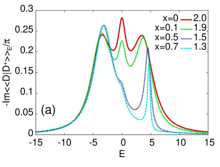
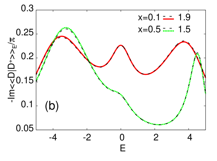
Figure 1: (color online) The transport GF of the model at hand is found to be symmetric with respect to $x=1$ to a very good approximation. In panel (a) we show the symmetry for the imaginary part of the transport GF, calculated for a few values of $x$ (as indicated) and $2-x$ (overlapping dashed curves). The differences between the two curves at particular values of the energy are smaller than $1\%$. Panel (b) shows the detailed behavior for $x=0.1$ vs. 1.9, and $x=0.5$ vs. 1.5, in the region where the differences are largest. The other parameters are $\varepsilon_{d}=-4$, $U=8$, and $T=0.3$.

The direct usage of Fermi’s golden rule,

$$\tilde{\gamma}_{i}=2\pi\sum_{f}|\langle f|V_{I}|i\rangle|^{2}\delta(E_{i}-E_{f}),$$ (29)

with $V_{I}$ being the tunneling part of the Hamiltonian (5), leads to the following expressions valid to second order in the dot coupling $V_{\lambda k\sigma}$:

$$\tilde{\gamma}^{\sigma}_{1} = \sum_{\lambda}\left(\Gamma^{\lambda}_{\sigma}[1-f_{\lambda}(\varepsilon_{\sigma})]+(1-x)^{2}\Gamma^{\lambda}_{{\sigma}}f_{\lambda}(\varepsilon_{{\sigma}}+U)\right)$$

$$\tilde{\gamma}_{2} = (1-x)^{2}\sum_{\lambda\sigma}\Gamma^{\lambda}_{\sigma}[1-f_{\lambda}(\varepsilon_{\sigma}+U)].$$ (31)

The last equation shows that the contribution from the doubly occupied states vanishes for $x=1$, as expected: for this value of $x$ the doubly occupied state is totally decoupled from the system.

IV Spectral and transport GFs: Numerical results and symmetry discussion

This section is devoted to the presentation of the results for the system in equilibrium, and for vanishing external magnetic field and spin-independent tunnelings. The transport coefficients can be calculated in the linear regime via Eqs. (14)–(16). In the following, all energies are measured in units of $\Gamma_{0}=\Gamma^{L}_{\downarrow}=\Gamma^{L}_{\uparrow}$. We start the discussion with the imaginary parts of the transport and spectral GFs, i.e., the transport and dot’s densities of states.

IV.1 The Green functions and their symmetry

A brief inspection of the formulae (19) and (25) for the transport and spectral GFs suggests that the former is symmetric with respect to changes of $x$ by $(2-x)$, while the latter is more difficult to judge due to a more complicated $x$ dependence. Thus we resort to numerical calculations and postpone further discussion of these formulae to the end of this section. In Figs. (1)–(5) we show the imaginary parts of both GFs as a function of energy for a number of $x$ values. The numerically perfect symmetry of the transport GF with respect to $x=1$ is visible in Fig. (1a). The imaginary part of the transport GF is plotted as function of energy for a number of $x$ and symmetry-related $(2-x)$ values. The (hardly visible) dashed black curves for the parameter $(2-x)$ overlap with the colored curves for $x$. Panel (b) of the figure is a magnification of the part of panel (a) close to the maxima, where the differences are largest. The observed differences are typically smaller than $1\%$.

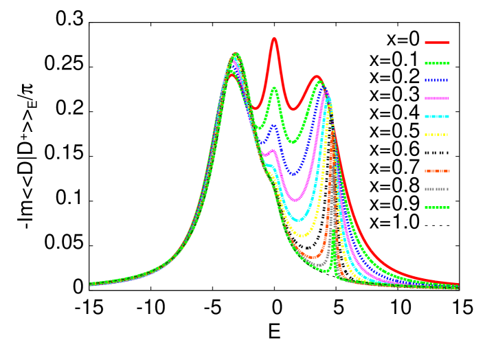
Figure 2: (color online) The imaginary part of the transport GF vs. energy $E$ for a number of $x$ values. For $x=1$ the doubly occupied state is blocked. This is visible as the disappearance of the upper Hubbard band. The other parameters for this particle-hole symmetric model read $\varepsilon_{d}=-4$, $U=8$, and $T=0.3$.

The systematic evolution of the transport density of states with changing $x$ is shown in Fig. (2). We present the results for $x\in[0,1]$ only, as the curves for the other values of $x$ are related by symmetry. For illustration we have assumed a particle-hole symmetric situation with $\varepsilon_{d}=-4$, $U=8$, and the same temperature for both leads, $T=0.3$. For these parameters and $x=0$, both transport and spectral GFs are identical, and the quantum dot is in the Kondo regime. Hence one observes the Abrikosov-Suhl resonance, also known as Kondo resonance, at the chemical potential $\mu=0$, and two Hubbard bands located symmetrically around zero energy. The occurrence of the Kondo effect in the particle-hole symmetric Hubbard model shows the power of the present version of the EOM technique supplemented with lifetime effects [26].

The increase of $x$ results in distinctive modifications of the transport density of states. First, one notices that the curves (for $x\neq 0$) are no longer particle-hole symmetric. Concomitant with this observation is the modification of the Kondo resonance, which develops a strong asymmetry with respect to the chemical potential ($E=0$). The lower Hubbard band changes rather weakly with $x$. Its height slightly increases, and the position slightly moves towards the chemical potential. Most dramatic changes are apparent in the upper Hubbard band, which strongly decreases with increasing $x$, getting narrower and finally vanishing completely for $x=1$. For the considered parameters the center of the upper Hubbard band moves slightly to the right in the figure. The result for $x=1$ requires additional comments. Let us note that the operator $D_{\sigma}$ for the doubly occupied state with $n_{\bar{\sigma}}=1$ vanishes. Under these conditions, the upper Hubbard band composed of the doubly occupied states does not contribute to transport.

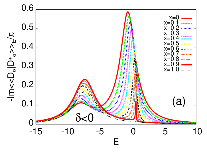
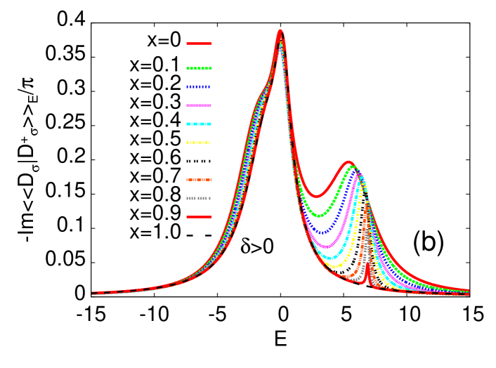
Figure 3: (color online) Panel (a) shows the transport density of states as a function of energy $E$ calculated for a set of $x$ values for negative $\delta=\varepsilon_{d}+U/2$, with $\varepsilon_{d}=-8$, $U=8$, and $T=0.3$. Panel (b) shows the similar evolution for $\delta=2>0$ and $\varepsilon_{d}=-2$.

In Figs. (1) and (2) we have shown the evolution of the transport density of states with $x$ for the particle-hole symmetric model for which $\delta=\varepsilon_{d}+U/2=0$. Non-zero values of $x$ break the particle-hole symmetry of the model. It turns out that for arbitrary values of $\delta$ the transport GF is symmetric with respect to $x$, albeit the differences are slightly larger than those in Fig. (1). Moreover, the effect of $x$ on the transport density of states varies depending on whether $\delta$ is positive or negative. In Fig. (3) we illustrate this for $U=8$ and two values of $\varepsilon_{d}$. In panel (a) of the figure we choose $\varepsilon_{d}=-8$, leading to negative value of $\delta=-4$. One can see that for this set of parameters the transport density of states $N_{\mathrm{tr}}(\mu)$ at the chemical potential ($\mu=0$) strongly changes with $x$. Both the absolute value and the slope are affected. Considering the formulae (15) and (16) for the transport parameters, which strongly depend on the transport density of states close to $E=0$, one expects for these parameters a noticeable changes of both conductance and thermopower with $x$. On the other hand, for the set of parameters used in the Fig. (3b), the transport GF for energies close to the chemical potential hardly changes with $x$; thus both conductance and thermopower are expected to vary only slightly with $x$. The symmetry of the transport GF with respect to $x\leftrightarrow 2-x$ ensures, as we shall see in the next section, the same symmetry of the transport coefficients.

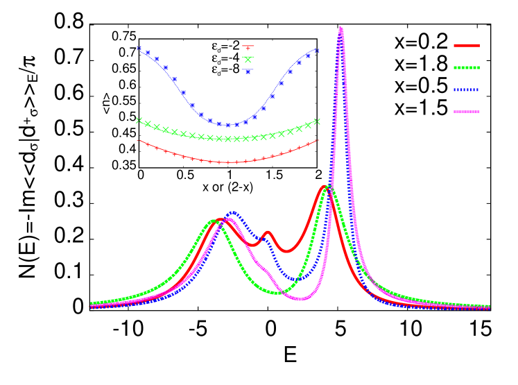
Figure 4: (color online) The dot’s spectral density of states, $N(E)=-({1}/{\pi})\mathrm{Im}\langle\langle d_{\sigma}|d^{\dagger}_{\sigma}\rangle\rangle_{E}$, vs. energy for several $x$ values. $N(E)$ changes with $x$ but is not symmetric, $N(E,x)\neq N(E,2-x)$. The other parameters are $\varepsilon_{d}=-4$, $U=8$, and $T=0.3$. The inset shows the $x$ dependence of the average occupation $\langle n\rangle$ per spin for $\varepsilon_{d}=-2,-4,-8$. For this quantity, the departures from perfect symmetry are very small. In order to increase their visibility, we plot the dependence $\langle n\rangle$ vs. $x$ as solid lines, and the dependence $\langle n\rangle$ vs. $(2-x)$ as points of the same color.

IV.2 The x vs. (2-x) symmetry in further detail

As argued in detail in [21], the model at hand is symmetric under the transformation $x\leftrightarrow 2-x$. However, we find that the (approximate) spectral GF derived above does not obey this symmetry, in contrast to the (approximate) transport GF. In particular, this deficiency is already apparent in the analytical formula for the spectral GF, Eq. (25). The departures from the $x\leftrightarrow 2-x$ symmetry are clearly visible in Fig. (4), where we show the density of states for $x=0.2$, 0.5, and the symmetry related values $(2-x)=1.8$, 1.5. The comparison of the curves obtained for the pairs of various $x$ (0.2 and 1.8, and 0.5 and 1.5, respectively) shows that the differences are largest for energies close to the chemical potential $\mu$, i.e., the point where the Kondo effect is expected. The differences at other energies seem to be related to those at $\mu$ by the sum rule, $\int_{-\infty}^{+\infty}dEN(E)=1$, which is always fulfilled with an accuracy better than $1\%$.

To obtain the above results, Fig. (4), we have used the formulae (25) and (26), which have been obtained, see the Suppl. Material [28], using the decoupling scheme I. As discussed there, we have tried several different decouplings. The others, i.e., II and III, overall lead to the same behavior with small quantitative changes only, hence we are not showing the results for them here. For the discussion of decouplings II and III, and also a calculation scheme different from that presented in Sec. III, see App. D and App. E below.

Interestingly, despite the asymmetry of the spectral GF, the average charge density per spin is symmetric under $x\leftrightarrow 2-x$. For a symmetrically coupled ($\Gamma^{L}=\Gamma^{R}$) quantum dot in equilibrium, the expression for the average occupation reduces to an integral of $N(E)$ weighted with the Fermi-Dirac distribution function. The dependence of $\langle n_{\sigma}\rangle=\langle n\rangle$ on $x$ is shown in the inset to Fig. (4) for $U=8$ and three values of $\varepsilon_{d}$, namely $-2$, $-4$, and $-8$. We see that the symmetry is obeyed with an accuracy of $\approx 0.01$, which is only slightly larger than the accuracy of the iterative computation: In the iterative process, $\langle n\rangle$ is used as a check of the accuracy of the solution, and we terminate the iteration when the change in $\langle n\rangle$ is less than 0.001 in consecutive steps.

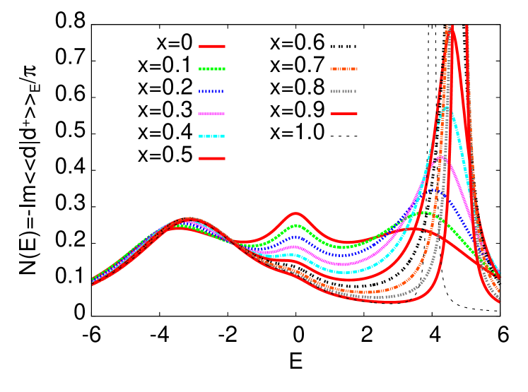
Figure 5: (color online) The dot’s density of states for a number of $x$ values. Note the weak changes of the lower Hubbard band with $x$, and the opposite behavior for the upper one. The other parameters are $\varepsilon_{d}=-4$, $U=8$, and $T=0.3$.

Anticipating the discussion in the next subsection, we expect in fact that the calculation of the spectral GF in the interval $0<x<1$ is, in the present approximation, more reliable than the results obtained for $1<x<2$. Hence we focus on the former regime, and illustrate in Fig. (5) in more detail the changes of the density of states with increasing $x$ for the particle-hole symmetric case, $\delta=0$. The general trends in the spectral GF for arbitrary $\delta$ are similar to those observed for the transport GF. The modifications of the lower Hubbard band are relatively small, while the Kondo peak and the upper Hubbard band are strongly modified with increasing $x$. The Kondo resonance disappears, and the upper Hubbard band gets narrower and higher with its center shifting initially towards higher energies.

IV.3 Remarks on the asymmetry of the spectral GF

A careful look at the spectral GF for $x=2$ in Fig. (6) shows that a small dip appears at the Fermi energy ($\mu=0$). Such a dip in the energy dependence of the equilibrium density of states at the chemical potential is a characteristic feature of all previous decouplings [38, 39] for the standard Hubbard model, (i.e., for $x=0$). The only approach which cures the deficiency is that of Lavagna [26] for the Hubbard model, which is applied here for the correlated-hopping model. Why does the approach fail at $x=2$? To elucidate the reason why Lavagna’s approach is not effective for the spectral function at $x=2$, we have to recall that the existence of the Kondo resonance for the Hubbard model in her approach is intimately related to the lifetime effects, i.e., the use of the parameters $\tilde{\gamma}^{(1)}_{\sigma}$, $\tilde{\gamma}^{(2)}$ as discussed earlier [26].

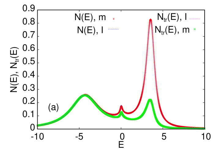
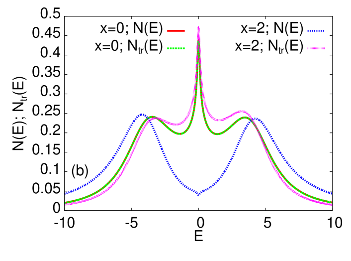
Figure 6: (color online) (a) Comparison of the spectral and transport densities of states for $x=0.5$ and $\varepsilon_{d}=-5$, $U=8$, and $T=0.03$ calculated by two methods: ‘m’ stands for the matrix method, while ‘I’ for decoupling I. Panel (b) illustrates the symmetry between these quantities for the particle-hole symmetric system with $\varepsilon_{d}=-4$, $U=8$, and $T=0.3$ calculated by the matrix method. For the full discussion of this figure, see App. E.

First we note that the explicit dependence on $x$ in the formulae (19) and (20) for the transport GF is through the factors $x(2-x)$ or $(x-1)^{2}$. The former vanishes for $x=0$ and $x=2$, and the latter is symmetric with respect to $x=1$. On the other hand, the inspection of the formula (25) for the spectral GF shows that for $x=0$ all extra terms vanish, while for $x=2$ they do not but rather give a large contribution to the self-energies $b_{1\bar{\sigma}},\Sigma^{T}_{1\bar{\sigma}}$, and $b_{2\bar{\sigma}},\Sigma^{T}_{2\bar{\sigma}}$. These self-energies at low $T$ lead to logarithmically divergent contributions close to the Fermi energy. For $x=0$, however, the divergent contributions from those terms which remain in $B_{d}$ and $n^{d}_{\mathrm{eff}}$ are cut off by the lifetime effects. On the other hand, this is not the case for $x=2$, and a number of diverging self-energies remain.

With this insight, we expect that in order to obtain the correct symmetry of the spectral GF one has to calculate, instead of projecting, those GFs which contain two lead operators. A careful inspection of the decoupling procedures shows, in fact, that the problem lies in the vanishing of certain contributions for $x=0$ but not for $x=2$. Thus, in order to render the expression for $\langle\langle d_{\sigma}|d^{\dagger}_{\sigma}\rangle\rangle_{\omega}$ symmetric, extra terms are needed. These can only result from higher-order contributions to the $S_{n,d,c}^{\mathrm{sp}}$ terms. As already noted, the calculations of these “missing” terms can, in principle, be performed in full analogy to previous calculations for the Hubbard model [37], but for the model at hand they are very complicated and will not be pursued here. Thus we conclude that contrary to the Hubbard model, where lifetime effects [26] can mimic the role of the fourth order terms [37], the symmetry of the spectral function of the correlated-hopping model requires calculations up to fourth order in the tunneling amplitude.

V Transport characteristics

V.1 Charge and heat conductance, and thermopower: linear regime

We emphasize again that all transport coefficients depend on the transport GF only, and hence fulfil the required $x$ symmetry. We focus the following discussion on the conductance $G$, the thermopower $S$, and the Wiedemann-Franz ratio $L=\kappa/(GT)$. In agreement with the preceding discussion, the nearly perfect $x$ vs. $(2-x)$ symmetry is very well visible in $G$ and $S$. In Fig. (7) we show the linear conductance $G$ and the thermopower $S$: the comparison of these quantities vs. $x$ (solid curves) and vs. $(2-x)$ shows that the symmetry is well obeyed. In Fig. (7) the symmetry is illustrated for the model with $\delta=0$, but it is also valid for arbitrary values of this parameter. For non-vanishing values of $\delta$ the functional dependence of $G(x)$ vs. $x$ differs but the symmetry remains intact. Interestingly, the overall dependence of the conductance on $x$ shown in Fig. (8) is similar to that in the previous figure. In both cases the conductance takes on maximal values for $x=0$ and $x=2$. However, it has to be noted that the behavior of $G(x)$ in the particle-hole symmetric case (shown in Fig. (7)) is due to the destructive effect of $x$ on the Kondo peak at the chemical potential. An increase of $x$ destroys the Kondo resonance, which leads to a smaller conductance. On the contrary, for the parameters of Fig. (8) it is the upper band of the transport density of states which is located close to the chemical potential that gives the largest contribution to $G$. The modification of this part of the transport spectrum (as visible in Fig. (3a)) determines the $x$ dependence of $G$.

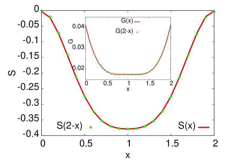
Figure 7: (color online) The linear thermopower $S$ (main panel) calculated for $\varepsilon_{d}=-4$, $U=8$, and $T=0.3$ vs. $x$. The inset shows the $x$-dependence of the linear conductance $G$. The solid lines indicate the thermopower (conductance) calculated for $0<x<1$, while the points correspond to the values obtained for $0<2-x<1$. The symmetry is nearly perfect in both cases.

The thermopower dependence on $x$ in the above two models is more complicated. In the first case, $S$ attains zero values for the perfectly symmetric transport densities of states at $x=0$ and $x=2$, and decreases for $x$ tending towards 1. The complicated sign changes of $S$ for the model with $\varepsilon_{d}=-8$, shown in Fig. (8a), can be approximately read off from the slope of the transport density of states shown in Fig. (3a). This is due to the fact that in the linear regime $S$ is proportional to the derivative of $N_{\mathrm{tr}}(E)$ taken at the chemical potential; cf. Eq. (18). We have also calculated the thermal conductance, and its dependence on $x$ traces the charge conductance. Thus we are not showing the plots here. Instead in Fig. (8b) the Wiedemann-Franz ratio $L=\kappa/(TG)$ normalised to the Lorenz number $L_{0}=(\pi^{2}/3)(k_{B}/e)^{2}$ is presented ($\kappa$ denotes the thermal conductance). One observes that for the parameters used the ratio is smaller than unity. This indicates a non-Fermi-liquid behavior of the system with hampered charge transport.

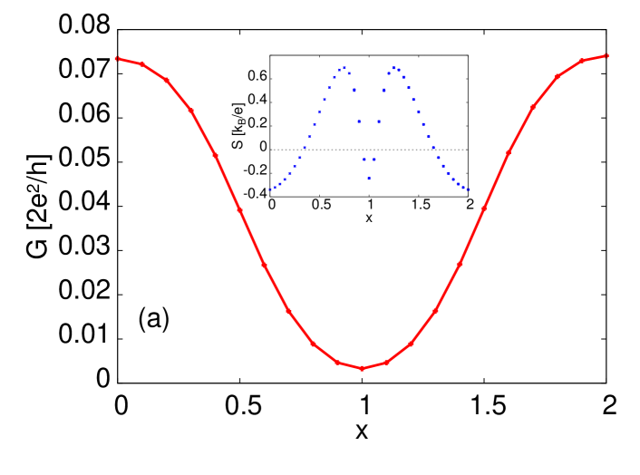
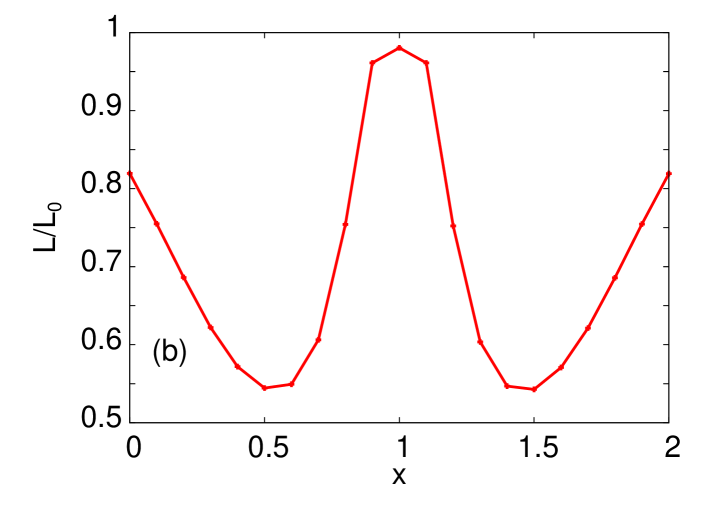
Figure 8: (color online) Conductance and thermopower $S$ (inset), as well as $L/L_{0}$ vs. $x$ as calculated for $\varepsilon_{d}=-8$, $U=8$, and $T=0.3$.

One of the most interesting questions related to the present study is the identification of measurable consequences of correlated hopping. In this context, it should be emphasized that one has experimental control over virtually all parameters of the devices under discussion. In particular, the gate bias independence of the parameters $\Gamma^{\lambda}$ demonstrated recently [40] for QDs fabricated using the electromigration technique, supports the hope to achieve this goal.

Naturally one would like to measure some transport characteristics of the system and infer the information about the actual value of $x$. The symmetry with respect to changing $x$ cannot serve the purpose, as this parameter most likely is beyond experimental control. However, other characteristics of the transport coefficients come to mind: namely the existence of the distinctive peaks in the conductance, and the concomitant saw-tooth shape of the thermopower.

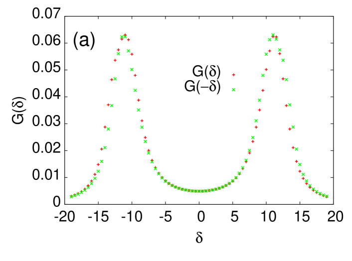
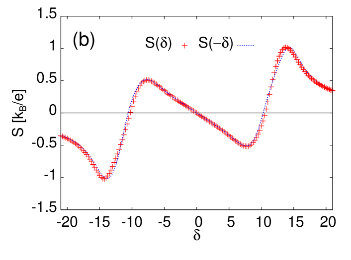
Figure 9: (color online) Symmetry of the transport coefficients with respect to gate bias (characterized by $\delta=\varepsilon_{d}+U/2$) for the model with $x=0$. Panel (a) shows the conductance, and (b) the thermopower. Other parameters are $U=22$, $T=0.5$.

The answer depends on whether one considers the linear or the strongly non-linear transport regime. In the linear case (we are interested in here), and for temperatures low on the scale of $\Gamma_{0}$, the transport parameters probe, as visible from Eqs. (14), the region of energy of the width of a few $k_{B}T$ in the vicinity of the chemical potential (here $\mu=0$), so the observed changes in the transport density of states are directly measurable (17). We claim that it is the $x$ dependent relative height of the two conductance peaks of the single-level quantum dot which gives direct information on the correlated-hopping term. The observed maxima of $G$, measured as function of gate bias, are related to the corresponding maxima in the transport density of states: one peak builds up when the on-dot energy band around $\varepsilon_{d}$ crosses the Fermi level ($\mu=0$), and the other when the upper Hubbard band centered around $2\varepsilon_{d}+U$ sweeps through $\mu$. For $x=0$ the two peaks are identical as visible in Fig. (9a). Similarly the corresponding “anti-symmetry” is observed for the thermopower, as visible in panel (b) of Fig. (9). This argumentation is applicable for a symmetrically coupled quantum dot, i.e., for $\Gamma^{L}=\Gamma^{R}$.

In Fig. (10a) we show the dependence of the conductance on gate bias, i.e., on $\varepsilon_{d}$, for a few values of $x$, namely $x=0$, 0.1, 0.2, 0.3, and 0.5. One observes a change of the relative height between the lower and the upper conductance “bands” with increasing $x$. The lower conductance peak decreases with $x$ while the upper one stays constant. The observed decrease is faster than linear as shown in the inset to the figure. The proportionality factor in the linear fit, here equal to 0.04, is not universal, but depends on the details. However, the decrease of the lower peak height with $x$ is a universal effect for a symmetrically coupled quantum dot, and gives immediate information on the very presence of the correlated-hopping contribution.

We emphasize that the observation of the different heights of the two consecutive conductance peaks in the two-terminal quantum dot provides a unique proof of the existence of correlated hopping. As we are studying a single-level quantum dot, the main condition related to experimentally studied devices is that the distance between consecutive levels in the dot has to be larger than the Coulomb repulsion $U$. Otherwise, the consecutive conductance peaks would correspond to singly occupied levels. This probably is the most serious condition to fulfil. Additional information can be drawn from the analysis of the thermopower. However, the gate bias dependence of $S$ is slightly more complicated, as is visible from Fig. (10b): An increase of $x$ leads to an increase of the amplitude of $S$ for $\delta$ values corresponding to the lower conductance peak, $\delta\approx-12$, while $S$ remains virtually unchanged for $\delta\approx+10$, corresponding to the upper conductance peak.

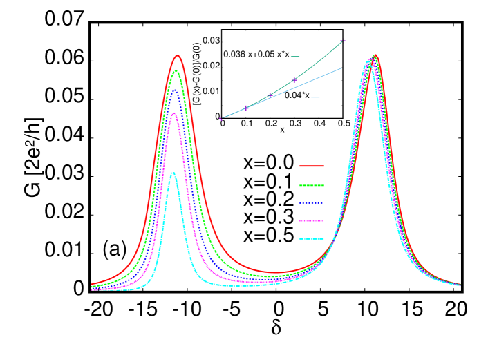
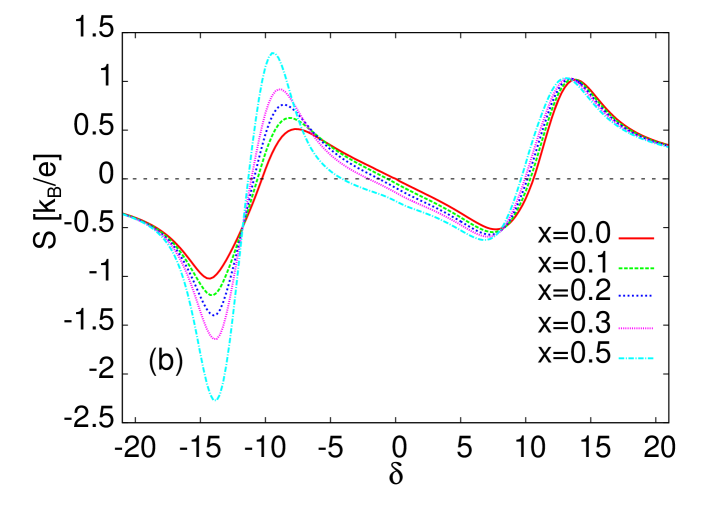
Figure 10: (color online) The effect of $x$ variation on the gate bias dependence (characterized by $\delta=\varepsilon_{d}+U/2$) of the conductivity, (a), and the thermopower, (b), for the model with $U=22$ at $T=0.5$. Increasing $x$ increases the asymmetry of the conductivity. The upper peak remains essentially intact while the height of the lower one decreases. The inset shows that the decrease of the height is faster than linear.

The effect of non-symmetric couplings on the conductance and the thermopower is shown in Fig. (11) for $\Gamma^{R}/\Gamma^{L}=2,3,4,6$. The anisotropy only weakly affects the lower conductance peak. Its effect on the upper peak is appreciable and includes a decrease of the magnitude and an increase of the width. The former effect masks the asymmetry in the peak heights induced by finite $x$, hence its unique identification becomes more difficult. However, the thermopower (Fig. (11b)) reacts in a more complicated way. Its overall amplitude diminishes in comparison to the symmetrically coupled dot, but both low and high $\delta$ parts are modified. The decrease of the magnitude of the thermopower variations can be understood by noting that $S$ is proportional to the slope of the conductivity at the corresponding energy, which is known as Mott relation.

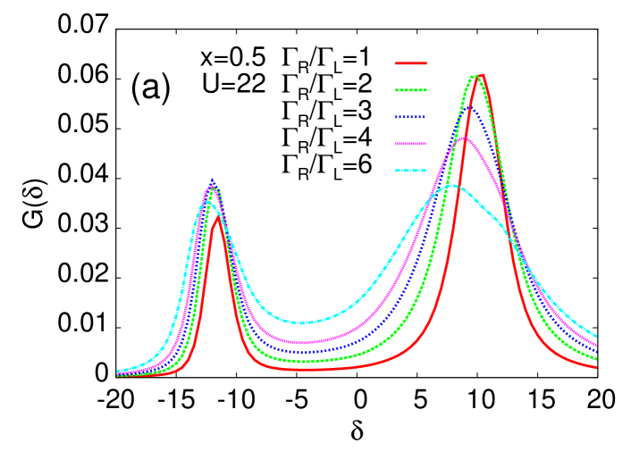
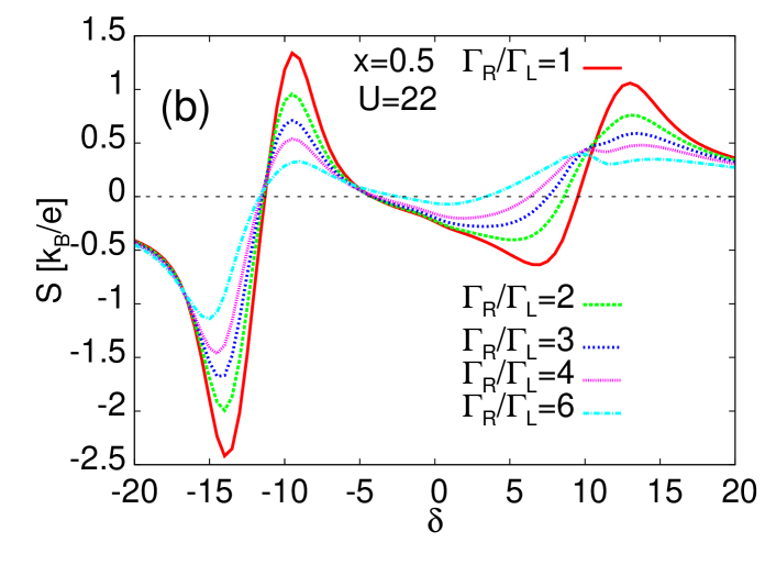
Figure 11: (color online) Dependence of (a) the linear conductance and (b) the thermopower on gate bias, characterized by $\delta=\varepsilon_{d}+U/2$, for $x=0.5$, $U=22$, and $T=0.5$. One observes only a small effect of the anisotropy of the couplings on the lower conductance peak, but large changes of the upper peak, namely a decrease of its height and an increase of its width when increasing the ratio $\Gamma^{R}/\Gamma^{L}$.

Our EOM results quantitatively agree with those obtained by the NRG technique [20, 21]. In particular, an increase of $x$ induces similar modifications of the conductance and thermopower in both methods. This is well seen by comparing, e.g., our Fig. (10) with panels (a) and (b) in Fig. 3 of [21]. It is more difficult to directly compare our results with those presented in [20], as these authors concentrate on such aspects as spin conductance and temperature dependencies. However, some curves shown in their Fig. 3 are close to our results for the corresponding set of parameters.

As a brief intermediate résumé, we note that all measurable characteristics exhibit the required symmetry properties. In particular, we have argued that a detailed experimental analysis of the gate bias dependence of both conductance and thermopower, in devices without orbital degeneracy and such that an adequate control of the symmetry of the couplings is feasible, may elucidate the role played by the correlated hopping, and may even allow for the extraction of $x$.

V.2 Non-linear conductance

The non-equilibrium Green function approach is well suited to treat finite voltages, since the EOM captures, albeit in a not well controlled way, higher-order scattering processes including those analysed in [41]. However, the full analysis of the conductance and other transport characteristics in the non-linear regime is beyond the scope of the present paper: these quantities not only depend on $x$, $\delta$, and $V$, but also on temperature, Coulomb interaction, and the anisotropy of the couplings.

Here we focus on the differential conductance, $G_{d}(x,\delta,V)={\partial I}/{\partial V}$. We present results for the dependence of $G_{d}$ on $x$ for $\delta=-4$ and a number of voltages $V$ (Fig. (12), panel (a)), and the dependence of $G_{d}$ on $\delta$ for $x=0.3$ (panel (b)). In both cases $U=8$ and $T=0.3$. The linear conductance, formally corresponding to $V=0$, is shown by red pluses. For a small voltage, $V=0.1$, the differences between small-voltage and zero-voltage results are small, but they strongly increase with $V$. The departures from the linear regime are more pronounced for small $x$ (and $2-x$), and close to the resonant values of the gate bias when the conductance is maximal.

For small values of $x$ and $2-x$, the changes of $G_{d}$ with $V$ are relatively large, but decrease for $x$ approaching $x=1$, see panel (a) in Fig. (12). These variations can be understood by recalling the full formula (6) for $I$, and noting that the spectral Green function entering it also depends on the voltage $V$ in a rather complicated way. For a finite voltage, the energy integration interval depends on temperature, but generally is of order $V$ at low $T$, thus the actual value of the current and the differential conductance depend on the detailed behavior of the transport spectral density in the considered energy interval. For $x=1$, the differences are very small, due to the rather smooth dependence of the transport spectral density on energy in the region between $\mu_{L}$ and $\mu_{R}$ (cf. Fig. (3)). It is worth noting that the $x\leftrightarrow 2-x$ symmetry of the conductance is valid also in the non-linear regime.

The asymmetry between the conductance peaks for positive and negative values of $\delta$, visible in panel (b) of Fig. (12), are related to the particle-hole symmetry breaking by the correlated hopping. The asymmetry depends on the actual value of $x$ and may thus be utilized in precise experiments to obtain information on its value.

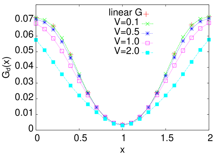
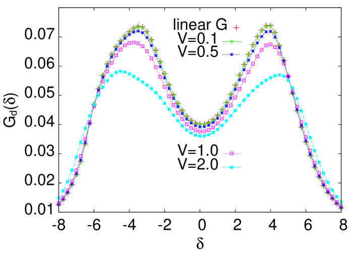
Figure 12: (color online) (a) Differential conductance $G_{d}$ versus $x$ for $\delta=-4$, $U=8$, $T=0.3$, and a few values of the voltage $V$ as indicated. Panel (b) shows the dependence of $G_{d}$ on $\delta=\varepsilon_{d}+U/2$ for $x=0.3$ and the same $U$ and $T$. In both panels the linear conductance is shown by red pluses.

VI Summary and conclusion

The transport of charge and heat via nanostructures consisting of a quantum dot (QD) coupled to two external normal electrodes has been studied by the non-equilibrium Green function (GF) technique in combination with the equation of motion (EOM) approach. The system is described by the Anderson Hamiltonian containing not only the standard single-particle tunneling term, but also an additional one of many-body origin, known in the literature as assisted or correlated hopping. This term, often neglected in the analysis of transport measurements of QD nanostructures, breaks the particle-hole symmetry of the model and thus may be important or even decisive for the interpretation of various experiments.

The correlated-hopping term, which we have characterized by the parameter $x$ ($0\leq x\leq 2$), modifies the tunneling part of the single-impurity model. Employing the non-equilibrium GF method to describe charge and heat transport, it becomes apparent that two different Green functions are needed: one of them, which we denote transport GF, enters the formulae for the charge and heat flux, while the other is related to the dot density of states and hence the dot’s average occupation. However, the equations for both GFs are coupled to each other via the occupation and certain self-energies. To obtain each of the GFs within the EOM technique, one has to project higher-order GFs, arising in the chain of EOMs, onto lower order ones. The simplest decoupling leads to a transport GF fulfilling the $x$ symmetry of the model. However, the spectral GF is found not to be symmetric under $x\leftrightarrow 2-x$. Attempting to cure this deficiency, we have tried three different decoupling schemes (see [28]), but failed to achieve the required symmetry. Even the calculation of the full matrix GF with various decouplings did not restore the $x$-symmetry. We argue that the symmetry restoration in the spectral GF $g^{r}(E)$ requires the inclusion of higher order GFs, thereby introducing higher powers of $x$. In contrast to the spectral GF, the dot occupation and all transport coefficients preserve the proper symmetry. Hence we are confident that the transport properties calculated in this work, and their parameter dependencies, are reliable.

The analytical approach employed here clarifies explicitly that for the description of the model with correlated hopping two characteristic Green functions are needed. One of them defines the transport through the system, and the other the thermodynamic properties, like the on-dot density of states or the occupancy of the dot. The intimate coupling between both GFs is realized $via$ the on-dot occupancy of the opposite-spin electrons and various self-energies. This, in conjunction with the general formulae for the currents, clearly shows the various ways the voltage $V$, the magnetic field $B$, and the temperature difference $\Delta T$ enter the transport characteristics.

However, one should note that within the EOM method not only many of the leading, but also some very-high-order contributions—in the sense of perturbation theory—are included, hence an interpretation of the results in terms of low-order processes (which can be quite illuminating, if applicable, see, e.g., Ref. [41]) is beyond reach.

In order to elucidate the role of correlated hopping, and find possible ways to infer its existence (and maybe even its value) from transport experiments, we studied in detail the spectral and transport properties of the QD system. The data presented in Fig. (9) show that the model for $x=0$ leads to a conductance symmetric and a thermopower anti-symmetric with respect to $\delta=0$. A sizeable value of $x$ implies a distinct asymmetry, namely different heights of the conductance peaks and clear changes in the thermopower. Thus we conclude that a thorough symmetry analysis of the consecutive peaks in the conductance, and of the related features in the thermopower, can provide information on the very existence of the correlated hopping term as well as its magnitude. One of the conductance peaks of the single-level quantum dot is not affected by a change in $x$, while the other decreases in height. The increase of $[G(0)-G(x)]/G(0)$, where $G(0)$ is the conductance maximum at the upper peak and $G(x)$ its value at the lower peak, is faster than linear with $x$, i.e., faster than the function $y=a\cdot x$ ($a=0.04$ for the parameters in Fig. (10)). Measuring the peak variation and calculating the value of $a$ for the known parameters of the experimental setup hence allows for a conservative estimation of $x$ and thus the correlated-hopping term. Note that $\Gamma^{L}$ also can be estimated from experiment, as it is approximately given by the half-width of the upper conductance peak.

The anisotropy of the couplings affects the conductance and thermopower, as shown in Figs. (11a) and (11b), respectively. This figure exhibits the transport coefficients for a few values of the asymmetry (i.e., $\Gamma^{R}/\Gamma^{L}$) for $x=0.5$. An increase of this parameter mainly affects the half-width and the height of one of the peaks. In our setup, the impaired peak corresponds to large $\delta$. However, the anisotropy may mask the effect of the $x$ parameter, thus making its unique identification uncertain. However, as discussed above for a strongly asymmetric coupling the simultaneous measurement of the gate bias dependence of the thermopower provides additional information from which the very existence of a non-zero $x$ can be inferred.

The non-equilibrium Green function technique in conjunction with the EOM allows the study of transport coefficients beyond the linear approximation, as exemplified above. In this paper, we have limited ourselves to calculations of the differential conductance: the dependence of $G_{d}$ on $x$ and $\delta$ for a number of voltages is shown in Sec. V.2. The departures from the linear (small voltage) results depend on $x$ and $\delta$ in a complicated way. However, for the studied parameter values the conductance decreases with increasing $V$, except in the limits of a nearly empty or doubly occupied dot, i.e., at the outer wings of the conductance peaks. This is well visible in panel (b) of Fig. (12) for $\delta\lesssim-6$ and $\delta\gtrsim 6$.

Appendix A Charge and heat currents

The charge current out of the electrode $\lambda$ is calculated as time derivative of the average charge in that electrode [42, 43], $\langle N_{\lambda}\rangle=\sum_{k\sigma}\langle n_{\lambda{k}\sigma}\rangle$:

$$I_{\lambda}=-e\left\langle\frac{dN_{\lambda}}{dt}\right\rangle=\frac{ie}{\hbar}\langle[N_{\lambda},\hat{H}]\rangle$$ (32)

where $\langle...\rangle$ denotes the statistical average. The calculation of the heat flux follows that of the charge. The heat flux is

$$J_{\lambda}=\frac{i}{\hbar}\langle[H_{\lambda},\hat{H}]\rangle-\mu_{\lambda}\frac{i}{\hbar}\langle[N_{\lambda},\hat{H}]\rangle,$$ (33)

where $H_{\lambda}=\sum_{{k}\sigma}\varepsilon_{\lambda{k}\sigma}n_{\lambda{k}\sigma}$ is the energy operator for the electrode $\lambda$. Calculating the commutators and introducing appropriate GFs, one finds

$$I_{\lambda}(t) = \frac{2e}{\hbar}\sum_{{k}\sigma}{\rm Re}\bigg{[}{V}_{\lambda{k}\sigma}G^{<}_{\sigma,\lambda{k}\sigma}(t,t)\bigg{]},$$ (34)

$$J_{\lambda}(t) = \frac{2e}{\hbar}\sum_{{k}\sigma}(\varepsilon_{\lambda{k}}-\mu_{\lambda}){\rm Re}\bigg{[}{V}_{\lambda{k}\sigma}G^{<}_{\sigma,\lambda{k}\sigma}(t,t)\bigg{]}.$$ (35)

Here the GF $G^{<}_{\sigma,\lambda{k}\sigma}(t,t^{\prime})=i\langle c^{\dagger}_{\lambda k\sigma}(t^{\prime})D_{\sigma}(t)\rangle$ denotes the lesser GF. Using the standard approach [32] to calculate time-ordered functions, one obtains the final expressions for the stationary currents in the following general form:

$$I_{\lambda} = \frac{ie}{\hbar}\int\frac{dE}{2\pi}\sum_{\sigma}\Gamma_{\sigma}^{\lambda}(E)\{G_{\sigma}^{<}(E)$$ (36)

$$+ f_{\lambda}(E)[G_{\sigma}^{r}(E)-G_{\sigma}^{a}(E)]\},$$

$$J_{\lambda} = \frac{ie}{\hbar}\int\frac{dE}{2\pi}\sum_{\sigma}\Gamma_{\sigma}^{\lambda}(E)(E-\mu_{\lambda})\{G_{\sigma}^{<}(E)$$ (37)

$$+ f_{\lambda}(E)[G_{\sigma}^{r}(E)-G_{\sigma}^{a}(E)]\}.$$

The parameters $\Gamma_{\sigma}^{\lambda}(E)=2\pi\sum_{{k}}|V_{\lambda{k}\sigma}|^{2}\delta(E-\varepsilon_{\lambda{k}})$ describe the coupling between the dot and the electrode, and we write the equations for the stationary currents via Fourier transforms of the GFs $G^{i}_{\sigma}(E)=\langle\langle D_{\sigma}|D^{\dagger}_{\sigma}\rangle\rangle^{i}_{E}$ with $i=r,a,<$ denoting retarded, advanced, and lesser functions. Since the GFs $G^{i}_{\sigma}(E)=\langle\langle D_{\sigma}|D^{\dagger}_{\sigma}\rangle\rangle^{i}_{E}$ determine the transport properties of the system, we call them transport GFs in the following. On the other hand, it is important to note that the spectral properties of the dot (like the density of states) are given by another GF, defined with the operators $d_{\sigma}$ and $d^{\dagger}_{\sigma}$, namely $g_{\sigma}(E)=\langle\langle d_{\sigma}|d^{\dagger}_{\sigma}\rangle\rangle_{E}$. For example, the dot spectral function $A_{\sigma}(E)$ at energy $E$ is given as $A_{\sigma}(E)=-\mathrm{Im}g_{\sigma}(E+i0)/\pi$, and the equilibrium charge density $\langle n_{\sigma}\rangle$ equals the integral $\int dEA_{\sigma}(E)f(E)$, where $f(E)$ is the Fermi distribution at temperature $T$ and chemical potential $\mu$.

Having in mind non-equilibrium charge and heat transport induced by a voltage or a temperature difference across the system, we keep the dependence of the Fermi distribution functions $f_{\lambda}(E)$ on the electrode at hand via its chemical potential $\mu_{\lambda}$ and temperature $T_{\lambda}$. The heat current (37) can be written as difference between the energy current $J^{E}_{\lambda}$ and the charge current $I_{\lambda}$:

$$J_{\lambda}=J^{E}_{\lambda}-\mu_{\lambda}I_{\lambda}.$$ (38)

The standard application of the EOM technique gives retarded and advanced GFs. To calculate the currents, one also needs the lesser GF $G_{\sigma}^{<}(E)$ entering (36) and (37). In the literature various proposals have been used to obtain this function, some of them relying on the approximate calculations, others making use of proportionate couplings [42] $\Gamma_{\sigma}^{L}(E)=\alpha\Gamma_{\sigma}^{R}(E)$ with $\alpha=$ const. Here we shall present an expression which relates the transport lesser GF exactly to its retarded and advanced counterparts; the relation is exact in the wide-band limit. In this limit, the effective couplings $\Gamma^{\lambda}_{\sigma}(E)=\Gamma^{\lambda}_{\sigma}$ do not depend on energy, and one finds (see the Suppl. Material [28] for details):

$$\langle D^{\dagger}_{\sigma}D_{\sigma}\rangle = -i\int\frac{dE}{2\pi}G^{<}(E)$$

$$= i\int\frac{dE}{2\pi}\frac{\sum_{\lambda}\Gamma_{\sigma}^{\lambda}f_{\lambda}(E)}{\sum_{\lambda}\Gamma_{\sigma}^{\lambda}}[G^{r}_{\sigma}(E)-G^{a}_{\sigma}(E)].$$

This sum rule for the correlated-hopping model, which is exact in the wide-band limit, is an important formal result of our paper. Its proof is given in the Suppl. Material [28]. The sum rule (A) extends that found earlier [26] for the standard single-impurity Anderson model.

Using the above result for the lesser GF, one finds the currents flowing out of the $\lambda$ electrode as follows:

$$I_{\lambda} = \frac{2e}{\hbar}\int\frac{dE}{2\pi}\sum_{\sigma}\Gamma_{\sigma}^{\lambda}$$ (40)

$$\times \frac{\sum_{\lambda^{\prime}}\Gamma^{\lambda^{\prime}}_{\sigma}(f_{\lambda^{\prime}}(E)-f_{\lambda}(E))}{\sum_{\lambda^{\prime}}\Gamma^{\lambda^{\prime}}_{\sigma}}\mathrm{Im}G_{\sigma}^{r}(E),$$

$$J_{\lambda} = \frac{2e}{\hbar}\int\frac{dE}{2\pi}\sum_{\sigma}\Gamma_{\sigma}^{\lambda}(E)(E-\mu_{\lambda})$$ (41)

$$\times \frac{\sum_{\lambda^{\prime}}\Gamma^{\lambda^{\prime}}_{\sigma}(f_{\lambda^{\prime}}(E)-f_{\lambda}(E))}{\sum_{\lambda^{\prime}}\Gamma^{\lambda^{\prime}}_{\sigma}}\mathrm{Im}G_{\sigma}^{r}(E).$$

These expressions can be used for calculating the currents in an arbitrary system consisting of the central dot and several terminals.

Formally the above manipulations are similar to those arising in the calculation of the currents in the standard Anderson model [43]. However, here we deal with completely different GFs. Moreover, as we shall see below, to calculate the transport GF one also needs the spectral one. Note that the kinetic and transport coefficients are expressed through the imaginary part of the transport GF only. Due to this fact, we shall denote the imaginary part of the transport GF as “transport density of states”.

Appendix B Calculation of the transport Green function

Before calculating the relevant GF, let us note the following identities:

$$D_{\bar{\sigma}}D_{\sigma} = (1-x)d_{\bar{\sigma}}d_{\sigma},$$ (42)

$$n_{\bar{\sigma}}D_{\sigma} = (1-x)n_{\bar{\sigma}}d_{\sigma},$$ (43)

$$D_{\bar{\sigma}}n_{\sigma} = (1-x)d_{\bar{\sigma}}n_{\sigma},$$ (44)

$$D^{\dagger}_{\bar{\sigma}}c_{\lambda k\bar{\sigma}}D_{\sigma} = d^{\dagger}_{\bar{\sigma}}c_{\lambda k\bar{\sigma}}d_{\sigma},$$ (45)

which will be occasionally used in various formulae below. The above identities show that the point $x=1$ is a special one. Indeed, the model at hand is symmetric with respect to $x=1$ for $0\leq x\leq 2$. For $x=0$ the only hopping is that of single-particle type $V_{\lambda k\sigma}$, while for $n_{-\sigma}=1$ and $x=2$ one gets the effective hopping equal $-V_{\lambda k\sigma}$. This together with the fact that $V_{\lambda k\sigma}$ enters all formulae as $|V_{\lambda k\sigma}|^{2}$ explains the equivalence of the model at these two limiting points. We remark in passing that a similar change of sign of the effective hybridization is also observed in the periodic Anderson model [44]. The symmetry of the present model goes beyond these two points, $x=0,2$, and is valid for arbitrary $x\in[0,2]$ as discussed earlier [21]. It has to be stressed that within the present approach only the transport GF fulfils this symmetry, while the spectral one does not, as discussed in Sec. IV.

To find the transport GF, we apply the EOM technique to two-time GFs and perform the appropriate decoupling. The quality of the solution in this method depends on the decoupling procedure. Before proceeding, let us recall that the decouplings in the EOM technique typically are not well controlled. We shall benchmark the proposed approximation scheme by checking the symmetry of the solution with respect to changing $x\leftrightarrow 2-x$. We start with the calculation of the transport GF, but as will be evident higher-order GFs are needed to solve the system of equations. The coupling between various GFs is provided by some correlation functions, inter alia including the average occupation of the dot $\langle n_{\bar{\sigma}}\rangle$.

In Zubarev notation [33] for fermionic operators $A$ and $B$, the equation for the two-time GF written in frequency $\omega$ space reads

$$\omega\langle\langle A|B\rangle\rangle_{\omega}=\langle\{A,B\}\rangle+\langle\langle[A,H]|B\rangle\rangle_{\omega}.$$ (46)

Application of the above EOM to operators $A=D_{\sigma}$ and $B=D^{\dagger}_{\sigma}$ provides

$$[\omega-\varepsilon_{\sigma}]\langle\langle D_{\sigma}|D^{\dagger}_{\sigma}\rangle\rangle_{\omega}=1-x(2-x)\langle n_{\bar{\sigma}}\rangle+\sum_{\lambda k}V^{*}_{\lambda k\sigma}\langle\langle c_{\lambda k\sigma}|D^{\dagger}_{\sigma}\rangle\rangle_{\omega}+U\langle\langle n_{\bar{\sigma}}D_{\sigma}|D^{\dagger}_{\sigma}\rangle\rangle_{\omega}$$

$$-x(2-x)\sum_{\lambda k}\left[V^{*}_{\lambda k{\sigma}}\langle\langle n_{\bar{\sigma}}c_{\lambda k\sigma}|D^{\dagger}_{\sigma}\rangle\rangle_{\omega}+V^{*}_{\lambda k\bar{\sigma}}\langle\langle D^{\dagger}_{\bar{\sigma}}c_{\lambda k\bar{\sigma}}D_{\sigma}|D^{\dagger}_{\sigma}\rangle\rangle_{\omega}\right].$$ (47)

The EOM for the next GF,

$$(\omega-\varepsilon_{\lambda k})\langle\langle c_{\lambda k\sigma}|D^{\dagger}_{\sigma}\rangle\rangle_{\omega}=V_{\lambda k\sigma}\langle\langle D_{\sigma}|D^{\dagger}_{\sigma}\rangle\rangle_{\omega},$$ (48)

allows one to write

$$\sum_{\lambda k}V^{*}_{\lambda k\sigma}\langle\langle c_{\lambda k\sigma}|D^{\dagger}_{\sigma}\rangle\rangle_{\omega}=\Sigma_{0\sigma}(\omega)\langle\langle D_{\sigma}|D^{\dagger}_{\sigma}\rangle\rangle_{\omega}.$$ (49)

The factor in front of the GF on the rhs of the preceding equation defines the self-energy:

$$\Sigma_{0\sigma}(\omega)=\sum_{\lambda k}\frac{|V_{\lambda k\sigma}|^{2}}{\omega-\varepsilon_{\lambda k}}.$$ (50)

In the wide-band limit one approximates (50) by its imaginary part:

$$\Sigma_{0\sigma}(\omega)\approx-i\pi\sum_{\lambda k}{|V_{\lambda k\sigma}|^{2}}\delta(\omega-\varepsilon_{\lambda k})=-i\frac{1}{2}\sum_{\lambda}\Gamma_{\sigma}^{\lambda}(\omega)=-i(\Gamma^{L}_{\sigma}+\Gamma^{R}_{\sigma})/2=-i\bar{\Gamma}_{\sigma}/2,$$ (51)

typically assumed to be energy independent. The higher-order GF which multiplies $U$ in Eq. (47) reads

$$[\omega-\varepsilon_{\sigma}-U]\langle\langle n_{\bar{\sigma}}D_{\sigma}|D^{\dagger}_{\sigma}\rangle\rangle_{\omega}=(1-x)^{2}\langle n_{\bar{\sigma}}\rangle-\sum_{\lambda k}V_{\lambda k\bar{\sigma}}\langle\langle c^{\dagger}_{\lambda k\bar{\sigma}}D_{\bar{\sigma}}D_{\sigma}|D^{\dagger}_{\sigma}\rangle\rangle_{\omega}$$

$$+(1-x)^{2}\sum_{\lambda k}\left[V^{*}_{\lambda k\sigma}\langle\langle n_{\bar{\sigma}}c_{\lambda k\sigma}|D^{\dagger}_{\sigma}\rangle\rangle_{\omega}+V^{*}_{\lambda k\bar{\sigma}}\langle\langle D^{\dagger}_{\bar{\sigma}}c_{\lambda k\bar{\sigma}}D_{\sigma}|D^{\dagger}_{\sigma}\rangle\rangle_{\omega}\right].$$ (52)

Equation (52) suggests that the calculation of the transport GF, independently of the forthcoming decouplings, requires the knowledge of $\langle n_{\bar{\sigma}}\rangle$ and thus of the spectral GF, $\langle\langle d_{\bar{\sigma}}|d^{\dagger}_{\bar{\sigma}}\rangle\rangle_{\omega}$. The remaining GFs entering the rhs of Eqs. (47) and (52) fulfil

$$[\omega-\varepsilon_{\lambda k}]\langle\langle n_{\bar{\sigma}}c_{\lambda k\sigma}|D^{\dagger}_{\sigma}\rangle\rangle_{\omega}=V_{\lambda k\sigma}\langle\langle n_{\bar{\sigma}}D_{\sigma}|D^{\dagger}_{\sigma}\rangle\rangle_{\omega}-\sum_{\lambda^{\prime}k^{\prime}}V_{\lambda^{\prime}k^{\prime}\bar{\sigma}}\langle\langle c^{\dagger}_{\lambda^{\prime}k^{\prime}\bar{\sigma}}D_{\bar{\sigma}}c_{\lambda k\sigma}|D^{\dagger}_{\sigma}\rangle\rangle_{\omega}$$

$$+\sum_{\lambda^{\prime}k^{\prime}}V^{*}_{\lambda^{\prime}k^{\prime}\bar{\sigma}}\langle\langle D^{\dagger}_{\bar{\sigma}}c_{\lambda^{\prime}k^{\prime}\bar{\sigma}}c_{\lambda k\sigma}|D^{\dagger}_{\sigma}\rangle\rangle_{\omega},$$ (53)

$$[\omega-\varepsilon_{\lambda k}-\varepsilon_{\sigma}+\varepsilon_{\bar{\sigma}}]\langle\langle D^{\dagger}_{\bar{\sigma}}c_{\lambda k\bar{\sigma}}D_{\sigma}|D^{\dagger}_{\sigma}\rangle\rangle_{\omega}=\langle D^{\dagger}_{\bar{\sigma}}c_{\lambda k\bar{\sigma}}\rangle+V_{\lambda k\bar{\sigma}}\langle\langle n_{\bar{\sigma}}D_{\sigma}|D^{\dagger}_{\sigma}\rangle\rangle_{\omega}$$

$$-\sum_{\lambda^{\prime}k^{\prime}}V_{\lambda^{\prime}k^{\prime}\bar{\sigma}}\langle\langle c^{\dagger}_{\lambda^{\prime}k^{\prime}\bar{\sigma}}c_{\lambda k\bar{\sigma}}D_{\sigma}|D^{\dagger}_{\sigma}\rangle\rangle_{\omega}+\sum_{\lambda^{\prime}k^{\prime}}V^{*}_{\lambda^{\prime}k^{\prime}\sigma}\langle\langle D^{\dagger}_{\bar{\sigma}}c_{\lambda k\bar{\sigma}}c_{\lambda^{\prime}k^{\prime}\sigma}|D^{\dagger}_{\sigma}\rangle\rangle_{\omega},$$ (54)

$$[\omega+\varepsilon_{\lambda k}-\varepsilon_{\sigma}-\varepsilon_{\bar{\sigma}}-U]\langle\langle c^{\dagger}_{\lambda k\bar{\sigma}}D_{\bar{\sigma}}D_{\sigma}|D^{\dagger}_{\sigma}\rangle\rangle_{\omega}=(1-x)^{2}\langle c^{\dagger}_{\lambda k\bar{\sigma}}D_{\bar{\sigma}}\rangle+x(2-x)\langle c^{\dagger}_{\lambda k\bar{\sigma}}D_{\bar{\sigma}}n_{\sigma}\rangle-V^{*}_{\lambda k\bar{\sigma}}\langle\langle n_{\bar{\sigma}}D_{\sigma}|D^{\dagger}_{\sigma}\rangle\rangle_{\omega}$$

$$+(1-x)^{2}\sum_{\lambda^{\prime}k^{\prime}}\left[V^{*}_{\lambda^{\prime}k^{\prime}\sigma}\langle\langle c^{\dagger}_{\lambda k\bar{\sigma}}d_{\bar{\sigma}}c_{\lambda^{\prime}k^{\prime}\sigma}|D^{\dagger}_{\sigma}\rangle\rangle_{\omega}+V^{*}_{\lambda^{\prime}k^{\prime}\bar{\sigma}}\langle\langle c^{\dagger}_{\lambda k\bar{\sigma}}c_{\lambda^{\prime}k^{\prime}\bar{\sigma}}d_{\sigma}|D^{\dagger}_{\sigma}\rangle\rangle_{\omega}\right]$$

$$+x\sum_{\lambda^{\prime}k^{\prime}}\left[V^{*}_{\lambda^{\prime}k^{\prime}\sigma}\langle\langle c^{\dagger}_{\lambda k\bar{\sigma}}D_{\bar{\sigma}}n_{\sigma}c_{\lambda^{\prime}k^{\prime}\sigma}|D^{\dagger}_{\sigma}\rangle\rangle_{\omega}+V^{*}_{\lambda^{\prime}k^{\prime}\bar{\sigma}}\langle\langle c^{\dagger}_{\lambda k\bar{\sigma}}c_{\lambda^{\prime}k^{\prime}\bar{\sigma}}n_{\bar{\sigma}}D_{\sigma}|D^{\dagger}_{\sigma}\rangle\rangle_{\omega}\right].$$ (55)

With the auxiliary notation

$$S^{\mathrm{tr}}_{n} = \sum_{\lambda k}V^{*}_{\lambda k\sigma}\langle\langle n_{\bar{\sigma}}c_{\lambda k\sigma}|D^{\dagger}_{\sigma}\rangle\rangle_{\omega}$$ (56)

$$S^{\mathrm{tr}}_{d} = \sum_{\lambda k}V^{*}_{\lambda k\bar{\sigma}}\langle\langle D^{\dagger}_{\bar{\sigma}}c_{\lambda k\bar{\sigma}}D_{\sigma}|D^{\dagger}_{\sigma}\rangle\rangle_{\omega}$$ (57)

$$S^{\mathrm{tr}}_{c} = \sum_{\lambda k}V_{\lambda k\bar{\sigma}}\langle\langle c^{\dagger}_{\lambda k\bar{\sigma}}D_{\bar{\sigma}}D_{\sigma}|D^{\dagger}_{\sigma}\rangle\rangle_{\omega}$$ (58)

one finds

$$[\omega-\varepsilon_{\sigma}-\Sigma_{0\sigma}]\langle\langle D_{\sigma}|D^{\dagger}_{\sigma}\rangle\rangle_{\omega}=1-x(2-x)\langle n_{\bar{\sigma}}\rangle-x(2-x)(S^{\mathrm{tr}}_{n}+S^{\mathrm{tr}}_{d})+U\langle\langle n_{\bar{\sigma}}D_{\sigma}|D^{\dagger}_{\sigma}\rangle\rangle_{\omega}$$ (59)

$$[\omega-\varepsilon_{\sigma}-U]\langle\langle n_{\bar{\sigma}}D_{\sigma}|D^{\dagger}_{\sigma}\rangle\rangle_{\omega}=(1-x)^{2}\langle n_{\bar{\sigma}}\rangle-S^{\mathrm{tr}}_{c}+(1-x)^{2}(S_{n}^{\mathrm{tr}}+S_{d}^{\mathrm{tr}}).$$ (60)

We shall not calculate the GFs containing two $c_{\lambda k\sigma}$ operators but approximate the GFs in question, avoiding the appearance of functions which describe spin-flip processes. Thus we project higher-order GFs as follows:

$$\langle\langle c^{\dagger}_{\lambda^{\prime}k^{\prime}\bar{\sigma}}c_{\lambda k\bar{\sigma}}D_{\sigma}|D^{\dagger}_{\sigma}\rangle\rangle_{\omega}\approx\langle c^{\dagger}_{\lambda^{\prime}k^{\prime}\bar{\sigma}}c_{\lambda k\bar{\sigma}}\rangle\langle\langle D_{\sigma}|D^{\dagger}_{\sigma}\rangle\rangle_{\omega},$$ (61)

and

$$\langle\langle c^{\dagger}_{\lambda^{\prime}k^{\prime}\bar{\sigma}}D_{\bar{\sigma}}c_{\lambda k\sigma}|D^{\dagger}_{\sigma}\rangle\rangle_{\omega}\approx\langle c^{\dagger}_{\lambda^{\prime}k^{\prime}\bar{\sigma}}D_{\bar{\sigma}}\rangle\langle\langle c_{\lambda k\sigma}|D^{\dagger}_{\sigma}\rangle\rangle_{\omega},$$ (62)

$$\langle\langle c^{\dagger}_{\lambda k\bar{\sigma}}d_{\bar{\sigma}}c_{\lambda^{\prime}k^{\prime}\sigma}|D^{\dagger}_{\sigma}\rangle\rangle_{\omega}\approx\langle c^{\dagger}_{\lambda k\bar{\sigma}}d_{\bar{\sigma}}\rangle\langle\langle c_{\lambda^{\prime}k^{\prime}\sigma}|D^{\dagger}_{\sigma}\rangle\rangle_{\omega},$$ (63)

$$\langle\langle D^{\dagger}_{\bar{\sigma}}c_{\lambda^{\prime}k^{\prime}\bar{\sigma}}c_{\lambda k\sigma}|D^{\dagger}_{\sigma}\rangle\rangle_{\omega}\approx\langle D^{\dagger}_{\bar{\sigma}}c_{\lambda^{\prime}k^{\prime}\bar{\sigma}}\rangle\langle\langle c_{\lambda k\sigma}|D^{\dagger}_{\sigma}\rangle\rangle_{\omega},$$ (64)

$$\langle\langle D^{\dagger}_{\bar{\sigma}}c_{\lambda k\bar{\sigma}}c_{\lambda^{\prime}k^{\prime}\sigma}|D^{\dagger}_{\sigma}\rangle\rangle_{\omega}\approx\langle D^{\dagger}_{\bar{\sigma}}c_{\lambda k\bar{\sigma}}\rangle\langle\langle c_{\lambda^{\prime}k^{\prime}\sigma}|D^{\dagger}_{\sigma}\rangle\rangle_{\omega}.$$ (65)

As already alluded to, the above decouplings are analogous to those which in the context of standard Hubbard model are known as Lacroix decouplings [34]. The decoupling of the following GF,

$$\langle\langle c^{\dagger}_{\lambda^{\prime}k^{\prime}\bar{\sigma}}c_{\lambda k\bar{\sigma}}d_{\sigma}|D^{\dagger}_{\sigma}\rangle\rangle_{\omega}\approx\langle c^{\dagger}_{\lambda^{\prime}k^{\prime}\bar{\sigma}}c_{\lambda k\bar{\sigma}}\rangle\langle\langle d_{\sigma}|D^{\dagger}_{\sigma}\rangle\rangle_{\omega},$$ (66)

introduces a novel GF which has not appeared hitherto, namely $\langle\langle d_{\sigma}|D^{\dagger}_{\sigma}\rangle\rangle_{\omega}$. To obtain this one, we use an exact relation:

$$\langle\langle D_{\sigma}|D^{\dagger}_{\sigma}\rangle\rangle_{\omega}=\langle\langle d_{\sigma}|D^{\dagger}_{\sigma}\rangle\rangle_{\omega}-x\langle\langle d_{\sigma}n_{\bar{\sigma}}|D^{\dagger}_{\sigma}\rangle\rangle_{\omega},$$ (67)

deduced from the operator identity $D_{\sigma}=d_{\sigma}-xd_{\sigma}n_{\bar{\sigma}}$. If the GF at hand is multiplied by $(1-x)$, we can express it by the functions appearing on the lhs of Eqs. (59) and (60):

$$(1-x)\langle\langle d_{\sigma}|D^{\dagger}_{\sigma}\rangle\rangle_{\omega}=(1-x)\langle\langle D_{\sigma}|D^{\dagger}_{\sigma}\rangle\rangle_{\omega}+x\langle\langle n_{\bar{\sigma}}D_{\sigma}|D^{\dagger}_{\sigma}\rangle\rangle_{\omega}.$$ (68)

This closes the system of equations for $\langle\langle D_{\sigma}|D^{\dagger}_{\sigma}\rangle\rangle_{\omega}$, except that we still need the spectral GF to calculate $\langle n_{\bar{\sigma}}\rangle$. It is worth noting in advance that the spectral GF $\langle\langle d_{\sigma}|d^{\dagger}_{\sigma}\rangle\rangle_{\omega}$ turns out to be coupled back to the transport one and the function $\langle\langle n_{\bar{\sigma}}d_{\sigma}|D^{\dagger}_{\sigma}\rangle\rangle_{\omega}$.

The solution of (59) and (60) is a relatively easy task. First, using the presented decouplings, one calculates the parameters $S^{\mathrm{tr}}_{n}$, $S^{\mathrm{tr}}_{d}$, and $S^{\mathrm{tr}}_{c}$. For $S^{\mathrm{tr}}_{n}$ one finds

$$S^{\mathrm{tr}}_{n} = \Sigma_{0\sigma}\langle\langle n_{\bar{\sigma}}D_{\sigma}|D^{\dagger}_{\sigma}\rangle\rangle_{\omega}$$ (69)

$$+ \sum_{\lambda^{\prime}k^{\prime}\bar{\sigma}}\left[V^{*}_{\lambda^{\prime}k^{\prime}\bar{\sigma}}\langle D^{\dagger}c_{\lambda^{\prime}k^{\prime}\bar{\sigma}}\rangle-V^{*}_{\lambda^{\prime}k^{\prime}\bar{\sigma}}\langle c^{\dagger}_{\lambda^{\prime}k^{\prime}\bar{\sigma}}D_{\bar{\sigma}}\rangle\right]$$

$$\times \Sigma^{\prime}_{\sigma}(\omega)\langle\langle D_{\sigma}|D^{\dagger}_{\sigma}\rangle\rangle_{\omega},$$

where

$$\Sigma^{\prime}_{\sigma}(\omega)=\sum_{\lambda k}\frac{|V_{\lambda k\sigma}|^{2}}{(\omega-\varepsilon_{\lambda k})^{2}},$$ (70)

vanishes in the wide-band limit and for energy independent coupling, the approximation assumed to be valid here. Thus we end up with

$$S^{\mathrm{tr}}_{n}=\Sigma_{0\sigma}\langle\langle n_{\bar{\sigma}}D_{\sigma}|D^{\dagger}_{\sigma}\rangle\rangle_{\omega},$$ (71)

where we have omitted the frequency dependence of the self-energy $\Sigma_{0\sigma}(\omega)$. Occasionally we shall use this convention in the following. Let us note that the proposed decouplings of the GFs containing two operators describing the electrons on the leads provide a simple expressions for $S^{\mathrm{tr}}_{n,d,c}$ in terms of $\langle\langle D_{\sigma}|D^{\dagger}_{\sigma}\rangle\rangle_{\omega}$ and $\langle\langle n_{\bar{\sigma}}D_{\sigma}|D^{\dagger}_{\sigma}\rangle\rangle_{\omega}$ only. Later on we shall apply analogous decouplings to find the spectral GFs $\langle\langle d_{\sigma}|d^{\dagger}_{\sigma}\rangle\rangle_{\omega}$ and $\langle\langle n_{\bar{\sigma}}d_{\sigma}|d^{\dagger}_{\sigma}\rangle\rangle_{\omega}$.

The remaining two auxiliary parameters read

$$S^{\mathrm{tr}}_{d} = \tilde{b}_{1\bar{\sigma}}+\Sigma^{(1)}_{\bar{\sigma}}\langle\langle n_{\bar{\sigma}}D_{\sigma}|D^{\dagger}_{\sigma}\rangle\rangle_{\omega}$$ (72)

$$+ \left[\tilde{b}_{1\bar{\sigma}}\Sigma_{0\sigma}-\Sigma^{T}_{1\bar{\sigma}}\right]\langle\langle D_{\sigma}|D^{\dagger}_{\sigma}\rangle\rangle_{\omega},$$

$$S^{\mathrm{tr}}_{c} = \bar{b}_{2\bar{\sigma}}+\left[(1-x)^{2}\Sigma^{T}_{2\bar{\sigma}}+\bar{b}_{2\bar{\sigma}}\Sigma_{0\sigma}\right]\langle\langle D_{\sigma}|D^{\dagger}_{\sigma}\rangle\rangle_{\omega}$$ (73)

$$+ \left[x(2-x)\Sigma^{T}_{2\bar{\sigma}}-\Sigma^{(2)}_{\bar{\sigma}}\right]\langle\langle n_{\bar{\sigma}}D_{\sigma}|D^{\dagger}_{\sigma}\rangle\rangle_{\omega},$$

where the novel symbols denote the various “summed” correlation functions or self-energies. For example,

$$\tilde{b}_{1\bar{\sigma}}(\omega)=\sum_{\lambda k}\frac{V^{*}_{\lambda k\bar{\sigma}}\langle D^{\dagger}_{\bar{\sigma}}c_{\lambda k\bar{\sigma}}\rangle}{\omega-\varepsilon_{\lambda k}-\varepsilon_{1}+i\tilde{\gamma}^{\bar{\sigma}}_{1}},$$ (74)

and

$$\tilde{b}_{2\bar{\sigma}}(\omega)=\sum_{\lambda k}\frac{V_{\lambda k\bar{\sigma}}\langle c^{\dagger}_{\lambda k\bar{\sigma}}D_{\bar{\sigma}}\rangle}{\omega+\varepsilon_{\lambda k}-\varepsilon_{2}+i\tilde{\gamma}_{2}}.$$ (75)

Using the definition of the operator $D_{\sigma}$, the last correlation function can be split as, e.g., $\tilde{b}_{1\bar{\sigma}}(\omega)={b}_{1\bar{\sigma}}(\omega)-x{N}_{1\bar{\sigma}}(\omega)$, with obvious definitions of ${b}_{1\bar{\sigma}}(\omega)$ and ${N}_{1\bar{\sigma}}(\omega)$.

The other self-energies entering (72) and (73) are defined as

$$\Sigma^{T}_{1\bar{\sigma}}(\omega)=\sum_{\lambda k}\sum_{\lambda^{\prime}k^{\prime}}\frac{V^{*}_{\lambda k\bar{\sigma}}V_{\lambda^{\prime}k^{\prime}\bar{\sigma}}\langle c^{\dagger}_{\lambda^{\prime}k^{\prime}\bar{\sigma}}c_{\lambda k\bar{\sigma}}\rangle}{\omega-\varepsilon_{\lambda k}-\varepsilon_{1}+i\tilde{\gamma}^{\bar{\sigma}}_{1}},$$ (76)

$$\Sigma^{T}_{2\bar{\sigma}}(\omega)=\sum_{\lambda k}\sum_{\lambda^{\prime}k^{\prime}}\frac{V_{\lambda k\bar{\sigma}}V^{*}_{\lambda^{\prime}k^{\prime}\bar{\sigma}}\langle c^{\dagger}_{\lambda k\bar{\sigma}}c_{\lambda^{\prime}k^{\prime}\bar{\sigma}}\rangle}{\omega+\varepsilon_{\lambda k}-\varepsilon_{2}+i\tilde{\gamma}_{2}},$$ (77)

$$\Sigma^{(1)}_{\bar{\sigma}}=\sum_{\lambda k}\frac{|V_{\lambda k\bar{\sigma}}|^{2}}{\omega-\varepsilon_{\lambda k}-\varepsilon_{1}+i\tilde{\gamma}^{\bar{\sigma}}_{1}},$$ (78)

$$\Sigma^{(2)}_{\bar{\sigma}}=\sum_{\lambda k}\frac{|V_{\lambda k\bar{\sigma}}|^{2}}{\omega+\varepsilon_{\lambda k}-\varepsilon_{2}+i\tilde{\gamma}^{\bar{\sigma}}_{1}},$$ (79)

where the energies $\varepsilon_{1(2)}$ are defined as

$$\varepsilon_{1}=\varepsilon_{\sigma}-\varepsilon_{\bar{\sigma}}$$ (80)

$$\varepsilon_{2}=\varepsilon_{\sigma}+\varepsilon_{\bar{\sigma}}+U.$$ (81)

The symbols $\tilde{\gamma}^{\bar{\sigma}}_{1}$ and $\tilde{\gamma}_{2}$ refer to the inverse lifetimes of the singly (doubly) occupied states on the dot. For the standard Anderson model they have been found [26] to play an decisive role in assuring the proper Kondo behavior at low temperatures. They are also important here due to the same reasons.

The correlation function $\bar{b}_{2\bar{\sigma}}(\omega)$ is given by the following combination:

$$\bar{b}_{2\bar{\sigma}}(\omega)=(1-x)[(1-x)b_{2\bar{\sigma}}(\omega)+xN_{2\bar{\sigma}}(\omega)]$$

$$\equiv(1-x)\tilde{b}_{2\bar{\sigma}}.$$ (82)

Some of the self-energies are expressed by the transport and other by the spectral GF as shown in the Suppl. Material [28], but to calculate $\bar{b}_{2\bar{\sigma}}(\omega)$ one needs $\langle\langle n_{\bar{\sigma}}D_{\sigma}|D^{\dagger}_{\sigma}\rangle\rangle_{\omega}$. On the other hand, the calculation of $\tilde{b}_{2\bar{\sigma}}$ requires the knowledge of the closely related function $\langle\langle n_{\bar{\sigma}}d_{\sigma}|D^{\dagger}_{\sigma}\rangle\rangle_{\omega}$. Thus the whole set of GFs required to solve the self-consistent set of equations comprises functions of diagonal: $\langle\langle D_{\sigma}|D^{\dagger}_{\sigma}\rangle\rangle_{\omega}$, $\langle\langle d_{\sigma}|d^{\dagger}_{\sigma}\rangle\rangle_{\omega}$, and off-diagonal: $\langle\langle n_{\bar{\sigma}}d_{\sigma}|d^{\dagger}_{\sigma}\rangle\rangle_{\omega}$, $\langle\langle n_{\bar{\sigma}}D_{\sigma}|D^{\dagger}_{\sigma}\rangle\rangle_{\omega}$ character.

The solution of Eqs. (59) and (60) for the transport GF is now written in a closed form. Defining the auxiliary function

$$I_{D}(\omega)=\frac{U-x(2-x)(\Sigma_{0\sigma}+\Sigma^{(1)}_{\bar{\sigma}})}{\omega-\varepsilon_{\sigma}-U-(1-x)^{2}(\Sigma_{0\sigma}+\Sigma^{(1)}_{\bar{\sigma}})-\Sigma_{\bar{\sigma}}^{(2)}+x(2-x)\Sigma^{T}_{2\bar{\sigma}}},$$ (83)

which for $x=0$ reduces to $I_{d}$ (cf. Eq. (26) in the main text) [27], and finds

$$\langle\langle D_{\sigma}|D^{\dagger}_{\sigma}\rangle\rangle_{\omega}=\frac{1-x(2-x)(\langle n_{\bar{\sigma}}\rangle+\tilde{b}_{1\bar{\sigma}})+n^{D}_{\mathrm{eff}}(\omega)I_{D}(\omega)}{\omega-\varepsilon_{d}-\Sigma_{0\sigma}+x(2-x)(\tilde{b}_{1\bar{\sigma}}\Sigma_{0\sigma}-\Sigma^{T}_{1\bar{\sigma}})-I_{D}(\omega)B_{D}(\omega)},$$ (84)

with

$$n^{D}_{\mathrm{eff}}(\omega) = (1-x)^{2}(\langle n_{\bar{\sigma}}\rangle+\tilde{b}_{1\bar{\sigma}})-\bar{b}_{2\bar{\sigma}},$$ (85)

$$B_{D}(\omega) = (1-x)^{2}[\tilde{b}_{1\bar{\sigma}}\Sigma_{0\sigma}-\Sigma^{T}_{1\bar{\sigma}}-\Sigma^{T}_{2\bar{\sigma}}]-\bar{b}_{2\bar{\sigma}}\Sigma_{0\sigma},$$ (86)

and

$$\Sigma_{ndD}(\omega)=(1-x)^{2}(\Sigma_{0\sigma}+\Sigma^{(1)}_{\bar{\sigma}})-x(2-x)\Sigma^{T}_{2\bar{\sigma}}+\Sigma_{\bar{\sigma}}^{(2)}.$$ (87)

The related GF $\langle\langle n_{\bar{\sigma}}D_{\sigma}|D^{\dagger}_{\sigma}\rangle\rangle_{\omega}$ is given by

$$\langle\langle n_{\bar{\sigma}}D_{\sigma}|D^{\dagger}_{\sigma}\rangle\rangle_{\omega}=\frac{(1-x)^{2}(\langle n_{\bar{\sigma}}\rangle+\tilde{b}_{1\bar{\sigma}})-\bar{b}_{2\bar{\sigma}}}{\omega-\varepsilon_{\sigma}-U-\Sigma_{ndD}}+\frac{[(1-x)^{2}(\tilde{b}_{1\bar{\sigma}}\Sigma_{0\sigma}-\Sigma^{T}_{1\bar{\sigma}}-\Sigma^{T}_{2\bar{\sigma}})-\bar{b}_{2\bar{\sigma}}\Sigma_{0\sigma}}{\omega-\varepsilon_{\sigma}-U-\Sigma_{ndD}}\langle\langle D_{\sigma}|D^{\dagger}_{\sigma}\rangle\rangle_{\omega}.$$ (88)

Using the relations (43) and (82), we get the last required GF:

$$\langle\langle n_{\bar{\sigma}}d_{\sigma}|D^{\dagger}_{\sigma}\rangle\rangle_{\omega}=\frac{(1-x)(\langle n_{\bar{\sigma}}\rangle+\tilde{b}_{1\bar{\sigma}})-\tilde{b}_{2\bar{\sigma}}}{\omega-\varepsilon_{\sigma}-U-\Sigma_{ndD}}+\frac{[(1-x)(\tilde{b}_{1\bar{\sigma}}\Sigma_{0\sigma}-\Sigma^{T}_{1\bar{\sigma}}-\Sigma^{T}_{2\bar{\sigma}})-\tilde{b}_{2\bar{\sigma}}\Sigma_{0\sigma}}{\omega-\varepsilon_{\sigma}-U-\Sigma_{ndD}}\langle\langle D_{\sigma}|D^{\dagger}_{\sigma}\rangle\rangle_{\omega},$$ (89)

The various symbols used above are summarised in App. C, where they are also expressed in terms of the transport GFs and the auxiliary functions like (88) and (89). The calculation of the average occupation of the dot $\langle n_{\bar{\sigma}}\rangle$ requires the knowledge of the spectral GF (25). Also the self-energy $\tilde{b}_{1\bar{\sigma}}(\omega)$ requires the knowledge of the spectral GF and the related function $\langle\langle n_{\bar{\sigma}}d_{\sigma}|d^{\dagger}_{\sigma}\rangle\rangle$; cf. Eq. (99).

Appendix C Self-energies in terms of the Green functions

Here we list for completeness all self-energies entering the solutions expressed self-consistently in terms of the relevant GFs. The self-energy $\tilde{b}_{1\bar{\sigma}}(\omega)$ has been obtained in the previous section. It depends on the transport GF only:

$$\tilde{b}_{1\bar{\sigma}}(\omega)=\sum_{\lambda k}\frac{V^{*}_{\lambda k\bar{\sigma}}\langle D^{\dagger}_{\bar{\sigma}}c_{\lambda k\bar{\sigma}}\rangle}{\omega-\varepsilon_{\lambda k}-\varepsilon_{1}+i\tilde{\gamma}^{\bar{\sigma}}_{1}}$$

$$=\int\frac{d\varepsilon}{2\pi}\frac{\sum_{\lambda}\Gamma^{\lambda}_{\bar{\sigma}}f_{\lambda}(\varepsilon)\langle\langle D_{\bar{\sigma}}|D^{\dagger}_{\bar{\sigma}}\rangle\rangle^{a}_{\varepsilon}}{\omega-\varepsilon-\varepsilon_{1}+i\tilde{\gamma}^{\bar{\sigma}}_{1}}.$$ (90)

The calculation of $\bar{b}_{2\bar{\sigma}}(\omega)$ requires the knowledge of ${b}_{2\bar{\sigma}}(\omega)$ and ${N}_{2\bar{\sigma}}(\omega)$, which are expressed as

$$b_{2\bar{\sigma}}(\omega)=\sum_{\lambda k}\frac{V_{\lambda k\bar{\sigma}}\langle c^{\dagger}_{\lambda k\bar{\sigma}}d_{\bar{\sigma}}\rangle}{\omega+\varepsilon_{\lambda k}-\varepsilon_{2}+i\tilde{\gamma}_{2}}$$

$$=\int\frac{d\varepsilon}{2\pi}\frac{\sum_{\lambda}\Gamma^{\lambda}_{\bar{\sigma}}f_{\lambda}(\varepsilon)\langle\langle d_{\bar{\sigma}}|D^{\dagger}_{\bar{\sigma}}\rangle\rangle^{r}_{\varepsilon}}{\omega+\varepsilon-\varepsilon_{2}+i\tilde{\gamma}_{2}},$$ (91)

and

$$N_{2\bar{\sigma}}(\omega)=\sum_{\lambda k}\frac{V_{\lambda k\bar{\sigma}}\langle c^{\dagger}_{\lambda k\bar{\sigma}}d_{\bar{\sigma}}n_{\bar{\sigma}}\rangle}{\omega+\varepsilon_{\lambda k}-\varepsilon_{2}+i\tilde{\gamma}_{2}}$$

$$=\int\frac{d\varepsilon}{2\pi}\frac{\sum_{\lambda}\Gamma^{\lambda}_{\bar{\sigma}}f_{\lambda}(\varepsilon)\langle\langle n_{\sigma}d_{\bar{\sigma}}|D^{\dagger}_{\bar{\sigma}}\rangle\rangle^{r}_{\varepsilon}}{\omega+\varepsilon-\varepsilon_{2}+i\tilde{\gamma}_{2}}$$ (92)

At first glance the calculation of $b_{2\bar{\sigma}}(\omega)$ and $N_{2\bar{\sigma}}(\omega)$ requires two new GFs. However, it turns out that these quantities enter the formulae for the transport GFs in the combination $\bar{b}_{2\bar{\sigma}}(\omega)=(1-x)^{2}b_{2\bar{\sigma}}(\omega)+x(1-x)N_{2\bar{\sigma}}(\omega)$. Using their definitions and the relation (67), one arrives at

$$\bar{b}_{2\bar{\sigma}}(\omega)=(1-x)^{2}\int\frac{d\varepsilon}{2\pi}\frac{\sum_{\lambda}\Gamma^{\lambda}_{\bar{\sigma}}f_{\lambda}(\varepsilon)\langle\langle D_{\bar{\sigma}}|D^{\dagger}_{\bar{\sigma}}\rangle\rangle^{r}_{\varepsilon}}{\omega+\varepsilon-\varepsilon_{2}+i\tilde{\gamma}_{2}}$$

$$+x(2-x)\int\frac{d\varepsilon}{2\pi}\frac{\sum_{\lambda}\Gamma^{\lambda}_{\bar{\sigma}}f_{\lambda}(\varepsilon)\langle\langle n_{\sigma}D_{\bar{\sigma}}|D^{\dagger}_{\bar{\sigma}}\rangle\rangle^{r}_{\varepsilon}}{\omega+\varepsilon-\varepsilon_{2}+i\tilde{\gamma}_{2}}.$$ (93)

The remaining self-energies read

$$\Sigma^{T}_{1\bar{\sigma}}(\omega)=\sum_{\lambda k}\sum_{\lambda^{\prime}k^{\prime}}\frac{V^{*}_{\lambda k\bar{\sigma}}V_{\lambda^{\prime}k^{\prime}\bar{\sigma}}\langle c^{\dagger}_{\lambda^{\prime}k^{\prime}\bar{\sigma}}c_{\lambda k\bar{\sigma}}\rangle}{\omega-\varepsilon_{\lambda k}-\varepsilon_{1}+i\tilde{\gamma}^{\bar{\sigma}}_{1}}$$

$$=\int\frac{d\varepsilon}{2\pi}\frac{\sum_{\lambda}\Gamma^{\lambda}_{\bar{\sigma}}f_{\lambda}(\varepsilon)[1+\frac{i}{2}\Gamma_{\bar{\sigma}}\langle\langle D_{\bar{\sigma}}|D^{\dagger}_{\bar{\sigma}}\rangle\rangle^{a}_{\varepsilon}]}{\omega-\varepsilon-\varepsilon_{1}+i\tilde{\gamma}^{\bar{\sigma}}_{1}}$$ (94)

$$\Sigma^{T}_{2\bar{\sigma}}(\omega)=\sum_{\lambda k}\sum_{\lambda^{\prime}k^{\prime}}\frac{V_{\lambda k\bar{\sigma}}V^{*}_{\lambda^{\prime}k^{\prime}\bar{\sigma}}\langle c^{\dagger}_{\lambda k\bar{\sigma}}c_{\lambda^{\prime}k^{\prime}\bar{\sigma}}\rangle}{\omega+\varepsilon_{\lambda k}-\varepsilon_{2}+i\tilde{\gamma}_{2}}$$

$$=\int\frac{d\varepsilon}{2\pi}\frac{\sum_{\lambda}\Gamma^{\lambda}_{\bar{\sigma}}f_{\lambda}(\varepsilon)[1-\frac{i}{2}\Gamma_{\bar{\sigma}}\langle\langle D_{\bar{\sigma}}|D^{\dagger}_{\bar{\sigma}}\rangle\rangle^{r}_{\varepsilon}]}{\omega+\varepsilon-\varepsilon_{2}+i\tilde{\gamma}_{2}}$$ (95)

The following self-energies:

$$\Sigma^{(1)}_{\bar{\sigma}}=\sum_{\lambda k}\frac{|V_{\lambda k\bar{\sigma}}|^{2}}{\omega-\varepsilon_{\lambda k}-\varepsilon_{1}+i\tilde{\gamma}^{\bar{\sigma}}_{1}},$$ (96)

and

$$\Sigma^{(2)}_{\bar{\sigma}}=\sum_{\lambda k}\frac{|V_{\lambda k\bar{\sigma}}|^{2}}{\omega+\varepsilon_{\lambda k}-\varepsilon_{2}+i\tilde{\gamma}_{2}},$$ (97)

do not depend on the GFs and take on the limiting values $\Sigma_{0\sigma}$ if the inverse lifetimes $\tilde{\gamma}^{\bar{\sigma}}_{1}$ and $\tilde{\gamma}_{2}$ are positive infinitesimals $0^{+}$.

We have already seen the relation $\bar{b}_{2\bar{\sigma}}=(1-x)\tilde{b}_{2\bar{\sigma}}$. Even so it is possible to find the latter from the former, it is much more convenient to calculate $\tilde{b}_{2\bar{\sigma}}$ directly. The result reads

$$\tilde{b}_{2\bar{\sigma}}=(1-x)\int\frac{d\varepsilon}{2\pi}\frac{\sum_{\lambda}\Gamma^{\lambda}_{\bar{\sigma}}f_{\lambda}(\varepsilon)\langle\langle D_{\bar{\sigma}}|D^{\dagger}_{\bar{\sigma}}\rangle\rangle^{r}_{\varepsilon}}{\omega+\varepsilon-\varepsilon_{2}+i\tilde{\gamma}_{2}}$$

$$+x(2-x)\int\frac{d\varepsilon}{2\pi}\frac{\sum_{\lambda}\Gamma^{\lambda}_{\bar{\sigma}}f_{\lambda}(\varepsilon)\langle\langle n_{\sigma}d_{\bar{\sigma}}|D^{\dagger}_{\bar{\sigma}}\rangle\rangle^{r}_{\varepsilon}}{\omega+\varepsilon-\varepsilon_{2}+i\tilde{\gamma}_{2}},$$ (98)

and shows that its calculation requires the GF $\langle\langle n_{\sigma}d_{\bar{\sigma}}|D^{\dagger}_{\bar{\sigma}}\rangle\rangle^{r}_{\omega}$. It can be easily obtained from (88), and is given by (89).

Other self-energies are expressed in terms of the spectral GF:

$$b_{1\bar{\sigma}}(\omega)=\sum_{\lambda k}\frac{V^{*}_{\lambda k\bar{\sigma}}\langle d^{\dagger}_{\bar{\sigma}}c_{\lambda k\bar{\sigma}}\rangle}{\omega-\varepsilon_{1}+i\tilde{\gamma}^{\bar{\sigma}}_{1}}$$

$$=\int\frac{d\varepsilon}{2\pi}\frac{\sum_{\lambda}\Gamma^{\lambda}_{\bar{\sigma}}f_{\lambda}(\varepsilon)\langle\langle D_{\bar{\sigma}}|d^{\dagger}_{\bar{\sigma}}\rangle\rangle^{a}_{\varepsilon}}{\omega-\varepsilon-\varepsilon_{1}+i\tilde{\gamma}^{\bar{\sigma}}_{1}}.$$ (99)

In a similar manner one finds:

$$N_{1\bar{\sigma}}(\omega)=\sum_{\lambda k}\frac{V^{*}_{\lambda k\bar{\sigma}}\langle d^{\dagger}_{\bar{\sigma}}n_{\sigma}c_{\lambda k\bar{\sigma}}\rangle}{\omega-\varepsilon_{1}+i\tilde{\gamma}^{\bar{\sigma}}_{1}}$$

$$=\int\frac{d\varepsilon}{2\pi}\frac{\sum_{\lambda}\Gamma^{\lambda}_{\bar{\sigma}}f_{\lambda}(\varepsilon)\langle\langle D_{\bar{\sigma}}|d^{\dagger}_{\bar{\sigma}}n_{\sigma}\rangle\rangle^{a}_{\varepsilon}}{\omega-\varepsilon-\varepsilon_{1}+i\tilde{\gamma}^{\bar{\sigma}}_{1}}.$$ (100)

The definition $D_{\sigma}=d_{\sigma}-xn_{\bar{\sigma}}d_{\sigma}$ can be used to express $b_{1\bar{\sigma}}$ in terms of the spectral GF, $\langle\langle d_{\bar{\sigma}}|d^{\dagger}_{\bar{\sigma}}\rangle\rangle^{a}_{\omega}$, and the related one, $\langle\langle n_{\sigma}d_{\bar{\sigma}}|d^{\dagger}_{\bar{\sigma}}\rangle\rangle^{a}_{\omega}$.

Appendix D Spectral GF in other decoupling schemes

We have seen that the transport GF is symmetric with respect to $x=1$, while the spectral one lacks this property. Is this due to the simple decoupling procedure (decoupling I) we have applied? As discussed in detail in the Suppl. Material [28], there are a number of possibilities to decouple those higher-order GFs which contain products of two lead operators. In the paper [37] the GF of the standard Hubbard model has been calculated up to the order $|V_{\lambda k\sigma}|^{4}$. Such an approach requires calculations which avoid the decoupling of the GFs with two lead operators. Similar calculations for the present model are prohibitively difficult, thus we stick to the order $|V_{\lambda k\sigma}|^{2}$. However, even up to this order there is room for improvement in relation to the decoupling scheme. The decoupling I consists of the most natural projections of the higher-order GFs onto the lower order ones, as explained in Eqs. (61)–(66) for transport and analogous projections for spectral Green function.

The decoupling II (cf. Eqs. (30)–(33) in the Suppl. Material [28]) takes into account the spin and $x$-dependent shifts of the on-dot energies (Eqs. (40) and (41) in the Suppl. Material [28]). They can be expressed in terms of two lowest order GFs, see Eq. (52) in Ref. [28]. This decoupling formally modifies all self-energies but does not preclude an easy solution for the spectral GF. It still neglects the function $\langle\langle n_{\sigma}c_{\lambda k\sigma}|d^{\dagger}_{\sigma}\rangle\rangle^{r}_{\omega}$, which has not appeared hitherto. This function formally is of the same order as $\langle\langle n_{\bar{\sigma}}c_{\lambda k\sigma}|d^{\dagger}_{\sigma}\rangle\rangle^{r}_{\omega}$, and the hope is that taking it into account restores the symmetry. The inclusion of this GF introduces a fourth parameter which we denote $S^{\mathrm{sp}}_{\sigma}$. With the novel GF, one gets a $4\times 4$ matrix equation for the four parameters $S^{\mathrm{sp}}_{n,d,c,\sigma}$. However, it turns out that the inclusion of this GF only slightly changes the results, by introducing some asymmetries in both functions even for particle-hole symmetric systems. In summary, none of the seemingly more involved decouplings, presented in the Suppl. Material [28], leads to an improvement of the results with respect to the $x$ symmetry.

Appendix E Matrix formulation

As discussed in the Suppl. Material [28], one may have another look at the spectral and transport GFs, stemming from the definition of $D_{\sigma}=d^{\dagger}_{\sigma}(1-xn_{\bar{\sigma}})$. This allows to write

$$\langle\langle D_{\sigma}|D^{\dagger}_{\sigma}\rangle\rangle_{\omega} = \langle\langle d_{\sigma}|d^{\dagger}_{\sigma}\rangle\rangle_{\omega}$$ (101)

$$- x\langle\langle n_{\bar{\sigma}}d_{\sigma}|d^{\dagger}_{\sigma}\rangle\rangle_{\omega}-x\langle\langle d_{\sigma}|n_{\bar{\sigma}}d^{\dagger}_{\sigma}\rangle\rangle_{\omega}$$

$$+ x^{2}\langle\langle n_{\bar{\sigma}}d_{\sigma}|n_{\bar{\sigma}}d^{\dagger}_{\sigma}\rangle\rangle_{\omega},$$

and shows that to get both GFs one has to calculate a matrix GF formally consisting of $d_{\sigma}$ and $d_{\sigma}n_{\bar{\sigma}}$ operators only. The matrix GF reads ${\cal G}_{\sigma}=\langle\langle\phi_{\sigma}|\phi^{\dagger}_{\sigma}\rangle\rangle_{\omega}$ where $\phi=\{d_{\sigma},n_{\bar{\sigma}}d_{\sigma}\}^{\cal T}$, and ${\cal T}$ denotes the matrix transpose operation. The knowledge of ${\cal G}_{\sigma}$ is enough to get both spectral and transport GF. This formulation seems to be more symmetric compared to that used previously, and thus could, in principle at least, lead to the required symmetry not only of the transport but also the spectral GF.

The details of the calculations and the decouplings are presented in the Suppl. Material [28]. However, we have to stress again that the higher-order GFs appearing in all the entries of ${\cal G}_{\sigma}(\omega)$ have to be approximated. It turns out that the decoupling I applied to all four components of the matrix GF leads to results which are most symmetric and closest to the direct calculations presented in App. B. This is illustrated in panel (a) of Fig. (6) of the main text for $x=0.5$, and $\varepsilon_{d}=-5$, $U=8$, $T=0.03$. The differences between each set of curves obtained by the direct formulae (marked with I), and those obtained with the help of the matrix formulation (marked with “m”), are small, hardly visible for $x=0.5$; but they do depend on $x$ and are largest for $x=2$.

Panel (b) of of Fig. (6) shows the spectral and transport densities of states for two $x$ values, namely $x=0$ and $x=2$, calculated by the matrix method. One notices that in the matrix formulations the transport density of states for $x=2$ differs from that for $x=0$ also. This is related to the fact that in this method not only the charge density $\langle n_{\sigma}\rangle$ but the full spectral GF enters the formulae for the transport GF introducing some asymmetry. The comparison of the curves for $N(E)$ for $x=0$ and $x=2$ best illustrate the lack of the required symmetry in the spectral function. One of the main problems here is the complete suppression of the Kondo resonance in $g^{r}(\omega)$ for $x=2$. While the transport GF for $x=2$ is only quantitatively different from that calculated for $x=0$, the spectral functions at those two $x$ values are completely different with a minimum (for $x=2$) at the chemical potential where the Kondo resonance should appear. The source of the asymmetry is discussed in Sec. IV.3. The results shown in Fig. (6b) have been obtained from the matrix formulation, using decouplings of all four GFs analogous to decoupling I. The other two decouplings produce qualitatively similar results. In summary, none of the studied decoupling schemes leads to the appearance of the Kondo resonance in the spectral function for $x=2$.

References

- [1] A. P. Alivisatos, Semiconductor clusters, nanocrystals, and quantum dots, Science 271, 933 (1996).
- [2] N. A. Zimbovskaya and M. R. Pederson, Electron transport through molecular junctions, Phys. Rep. 509, 1 (2011).
- [3] G. Benenti, G. Casati, K. Saito, and R. S. Whitney, Fundamental aspects of steady-state conversion of heat to work at the nanoscale, Phys. Rep. 694, 1-124 (2017).
- [4] I. Ẑutic̀, J. Fabian, and S. Das Sarma, Spintronics: Fundamentals and applications Rev. Mod. Phys. 76, 323 (2004); T. Dietl and H. Ohno, Dilute ferromagnetic semiconductors: Physics and spintronic structures, Rev. Mod. Phys. 86, 187 (2014); S. A. Wolf, D. D. Awschalom, R. A. Buhrman, J. M. Daughton, S. von Molnar, M. L. Roukes, A. Y. Chtchelkanova, and D. M. Treger, Spintronics: A spin-based electronics vision for the future, Science 294, 1488 (2001).
- [5] M. Bayer, P. Hawrylak, K. Hinzer, et al., Coupling and entangling of quantum states in quantum dot molecules, Science 291, 451 (2001); Xuedong Hu and S. Das Sarma, Double quantum dot turnstile as an electron spin entangler, Phys. Rev. B 69, 115312 (2004); Y. Sherkunov, Jin Zhang, N. d’Ambrumenil, and B. Muzykantskii, Optimal electron entangler and single-electron source at low temperatures, Phys. Rev. B 80, 041313(R) (2009); N. Akopian, N. H. Lindner, E. Poem, Y. Berlatzky, J. Avron, D. Gershoni, B. D. Gerardot, and P. M. Petroff, Entangled photon pairs from semiconductor quantum dots, Phys. Rev. Lett. 96, 130501 (2006).
- [6] D. Loss and D. P. DiVincenzo, Quantum computation with quantum dots, Phys. Rev. A 57, 120 (1998); G. Burkard, H. A. Engel, and D. Loss, Spintronics and quantum dots for quantum computing and quantum communication, Fortschr. Phys. 48, 965 (2000); V. Cerletti, W. A. Coish, O. Gywat, et al., Recipes for spin-based quantum computing, Nanotech. 16, R27 (2005).
- [7] H.-A. Engel and D. Loss, Single-spin dynamics and decoherence in a quantum dot via charge transport, Phys. Rev. B 65, 195321 (2002); J. König and J. Martinek, Interaction-Driven Spin Precession in Quantum-Dot Spin Valves, Phys. Rev. Lett. 90, 166602 (2003); R. Świrkowicz, M. Wilczyński, and J. Barnaś, The Kondo effect in quantum dots coupled to ferromagnetic leads with noncollinear magnetizations: effects due to electron–phonon coupling, J. Phys.: Condens. Matter 20, 255219; C. A. Merchant and N. Marković, Electrically Tunable Spin Polarization in a Carbon Nanotube Spin Diode, Phys. Rev. Lett. 100, 156601 (2008); M. Hell, B. Sothmann, M. Leijnse, M. R. Wegewijs, and J. König, Spin resonance without spin splitting, Phys. Rev. B 91, 195404 (2015); N. M. Gergs, S. A. Bender, R. A. Duine, and D. Schuricht, Spin Switching via Quantum Dot Spin Valves, Phys. Rev. Lett. 120, 017701 (2018).
- [8] M. Di Ventra, Electrical Transport in Nanoscale Systems, Cambridge University Press, 2008.
- [9] J. Hubbard, Electron Correlations in Narrow Energy Bands, Proc. Royal Soc. London Ser. A, Mathematical and Physical Sciences 276, 238 (1963).
- [10] R. Micnas, J. Ranninger, and S. Robaszkiewicz, Superconductivity in a narrow-band system with intersite electron pairing in two dimensions. II. Effects of nearest-neighbor exchange and correlated hopping, Phys. Rev. B 39, 11653 (1989).
- [11] A. Hübsch, J. C. Lin, J. Pan, and D. L. Cox, Correlated Hybridization in Transition-Metal Complexes, Phys. Rev. Lett. 96, 196401 (2006).
- [12] M. M. Wysokiński, J. Kaczmarczyk, and J. Spałek, Correlation-driven d-wave superconductivity in Anderson lattice model: Two gaps, Phys. Rev. B 94, 024517 (2016).
- [13] R. Micnas, J. Ranninger, and S. Robaszkiewicz, Superconductivity in narrow-band systems with local nonretarded attractive interactions, Rev. Mod. Phys. 62, 113 (1990).
- [14] M. M. Wysokinski and J. Kaczmarczyk, Unconventional superconductivity in generalized Hubbard model: role of electron-hole symmetry breaking terms, J. Phys.: Condens. Matter 29, 085604 (2017).
- [15] M. Zegrodnik and J. Spałek, Universal properties of high-temperature superconductors from real-space pairing: Role of correlated hopping and intersite Coulomb interaction within the t-J-U model, Phys. Rev. B 96, 054511 (2017).
- [16] Y. Meir, K. Hirose, and N. S. Wingreen, Kondo Model for the 0.7 Anomaly in Transport through a Quantum Point Contact, Phys. Rev. Lett. 89, 196802 (2002).
- [17] F. Guinea, Effect of assisted hopping on the formation of local moments in magnetic impurities and quantum dots, Phys. Rev. B 67, 195104 (2003).
- [18] L. Borda and F. Guinea, Assisted hopping and interaction effects in impurity models, Phys. Rev. B 70, 125118 (2004).
- [19] T. Stauber and F. Guinea, Assisted hopping in the Anderson impurity model: A flow equation study, Phys. Rev. B 69, 035301 (2004).
- [20] J. C. Lin, F. B. Anders, and D. L. Cox, Influence of correlated hybridization on the conductance of molecular transistors, Phys. Rev. B 76, 115401 (2007).
- [21] B. Tooski, A. Ramsak, B. R. Bułka, and R. Zitko, Effect of assisted hopping on thermopower in an interacting quantum dot, New J. Phys. 16, 055001 (2014).
- [22] G. Gorski and K. Kucab, Influence of assisted hopping interaction on the linear conductance of quantum dot, Physica E 111, 190 (2019).
- [23] S. M. Cronenwett, H. J. Lynch, D. Goldhaber-Gordon, L. P. Kouwenhoven, C. M. Marcus, K. Hirose, N. S. Wingreen, and V. Umansky, Low-Temperature Fate of the 0.7 Structure in a Point Contact: A Kondo-like Correlated State in an Open System, Phys. Rev. Lett. 88, 226805 (2002).
- [24] L. H. Yu, Z. K. Keane, J. W. Ciszek, L. Cheng, J. M. Tour, T. Baruah, M. R. Pederson, and D. Natelson Kondo Resonances and Anomalous Gate Dependence in the Electrical Conductivity of Single-Molecule Transistors, Phys. Rev. Lett. 95, 256803 (2005).
- [25] T. A. Costi, Magnetic field dependence of the thermopower of Kondo-correlated quantum dots, Phys. Rev. B 100, 161106(R) (2019); Magnetic field dependence of the thermopower of Kondo-correlated quantum dots: Comparison with experiment, ibid. 100, 155126 (2019).
- [26] M. Lavagna, Transport through an interacting quantum dot driven out-of-equilibrium J. Phys. Conf. Ser. 592, 012141 (2015).
- [27] U. Eckern and K. I. Wysokiński, Two- and three-terminal far-from-equilibrium thermoelectric nanodevices in the Kondo regime, New J. Phys. 22, 013045 (2020).
- [28] Supplementary Material, available online at https://doi.org/10.5281/zenodo.5383227.
- [29] G. D. Mahan, Many-Particle Physics, Plenum, New York, 1981.
- [30] V. Zlatic and R. Monnier, Modern Theory of Thermoelectricity, Oxford University Press, Oxford, 2014.
- [31] N. W. Ashcroft and N. D. Mermin, Solid State Physics, Holt, Rinehart and Winston, New York, 1976, App. C.
- [32] H. Haug and A.-P. Jauho, Quantum Kinetics in Transport and Optics of Semiconductors, Second, Substantially Revised Edition, Springer, Berlin, 2008.
- [33] D. N. Zubarev, Usp. Fiz. Nauk 71, 71 (1960) [Engl. transl.: Sov. Phys. Usp. 3, 320 (1960)].
- [34] C. Lacroix, Density of states for the Anderson model, J. Phys. F: Metal Phys. 11, 2389 (1981).
- [35] A. Theumann, Self-Consistent Solution of the Anderson Model, Phys. Rev. 178, 978 (1969).
- [36] C. Lacroix, Density of states for the asymmetric Anderson model, J. Appl. Phys. 53, 2131 (1982).
- [37] R. Van Roermund, S.-Y. Shiau, and M. Lavagna, Anderson model out of equilibrium: Decoherence effects in transport through a quantum dot, Phys. Rev. B 81, 165115 (2010).
- [38] V. Kashcheyevs, A. Aharony, and O. Entin-Wohlman, Phys. Rev. B 73, 125338 (2006).
- [39] Miguel A. Sierra, Rosa López, and David Sánchez, Fate of the spin-1/2 Kondo effect in the presence of temperature gradients, Phys. Rev. B 96, 085416 (2017).
- [40] B. Dutta, D. Majidi, A. García Corral, P. A. Erdman, S. Florens, T. A. Costi, H. Courtois, and C. B. Winkelmann, Direct Probe of the Seebeck Coefficient in a Kondo-Correlated Single-Quantum-Dot Transistor, Nano Lett. 19, 506 (2019).
- [41] N. M. Gergs, Ch. B. M. Horig, M. R. Wegewijs, and D. Schuricht, Charge fluctuations in nonlinear heat transport Phys. Rev. B 91, 201107(R) (2015).
- [42] Y. Meir and N. S. Wingreen, Landauer Formula for the current through an interacting electron region, Phys. Rev. Lett. 68, 2512 (1992).
- [43] N. S. Wingreen and Y. Meir, Anderson model out of equilibrium: Noncrossing-approximation approach to transport through a quantum dot, Phys. Rev. B 49, 11040 (1994).
- [44] M. M. Wysokiński, M. Abram, and J. Spałek, Ferromagnetism in UGe2: A microscopic model, Phys. Rev. B 90, 081114(R) (2014).