Higher-order topological states
mediated by long-range coupling in $D_{4}$-symmetric lattices

Topological physics opens a door towards flexible routing and resilient localization of waves of various nature. Recently proposed higher-order topological insulators Benalcazar et al. (2017); Schindler et al. (2018a) provide advanced control over wave localization in the structures of different dimensionality. In many cases, the formation of such higher-order topological phases is governed by the lattice symmetries, with kagome Xue et al. (2018); Ni et al. (2018) and breathing honeycomb Wu and Hu (2015) lattices being prominent examples. Here, we design and experimentally realize the resonant electric circuit with $D_{4}$ symmetry and additional next-nearest-neighbor couplings. As we prove, a coupling of the distant neighbors gives rise to an in-gap corner state. Retrieving the associated invariant directly from the experiment, we demonstrate the topological nature of the designed system, revealing the role of long-range interactions in the formation of topological phases. Our results thus highlight the distinctions between tight-binding systems and their photonic counterparts with long-range couplings.

Higher-order topological insulators have recently emerged as a distinct class of topological systems implemented experimentally with various platforms, including crystalline solids Schindler et al. (2018b), phononic Serra-Garcia et al. (2018), acoustic Xue et al. (2018); Ni et al. (2018), and electromagnetic setups working at infrared Mittal et al. (2019); Hassan et al. (2019) and microwave Peterson et al. (2018); Li et al. (2020) frequencies, as well as resonant electric circuits Imhof et al. (2018); Serra-Garcia et al. (2019). Due to their ability to confine field in the structures of different dimensionality, such higher-order topological phases are promising candidates for topological resonators and lasers Bahari et al. (2017); Zhang et al. (2020); Han et al. (2020); Kim et al. (2020).

In many cases, the physics of such systems can be understood in terms of tight-binding models involving only the nearest neighbors’ interaction. However, this is not the case for photonics, where the long-range interactions of the individual meta-atoms can significantly alter the band structure Li et al. (2020).

Recently, several microwave experiments Chen et al. (2019); Xie et al. (2019) have demonstrated the emergence of corner states in the two-dimensional generalization of the celebrated Su-Schrieffer-Heeger model (SSH) with $D_{4}$ symmetry Liu and Wakabayashi (2017). At the same time, the respective tight-binding model [Fig. 1a] does not feature a zero-energy bandgap, and the associated corner state coexists with the continuum of the bulk modes [Fig. 1b].

In this Letter, we prove that the formation of zero-energy bandgap hosting topological corner states in $D_{4}$-symmetric systems crucially depends on the next-nearest-neighbor interaction, which facilitates the emergence of higher-order topological phase. To isolate the physics related to the next-nearest-neighbor coupling, we design and fabricate a sample based on a resonant LC circuit, where the magnitude of the coupling parameters can be flexibly controlled [Fig. 1c]. Besides the retrieval of frequencies and mode profiles of bulk, edge, and corner states, we also reveal generalized chiral symmetry of the model and calculate the topological invariant associated with $D_{4}$ lattice symmetry.

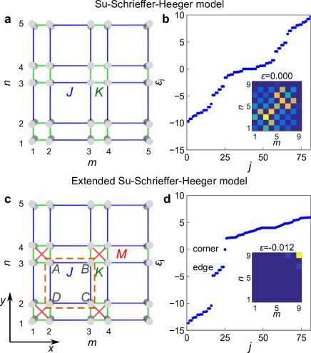
Figure 1: Extended two-dimensional Su-Schrieffer-Heeger model. a: Schematics of the two-dimensional SSH model realized as an array of nearest-neighbor-coupled resonators with the coupling strengths $J>0$ and $K>J$. b: Spectrum of energies $\varepsilon_{j}$ versus eigenvalue number $j$ for the model $9\times 9$ sites from panel a with couplings $J=1$, $K=4$. Inset shows the wavefunction for the eigenmode with $\varepsilon=0$. c: Proposed extension of 2D SSH with additional couplings $M>0$ in the strong-link unit cell. Orange dashed line shows the weak-link unit cell choice used for the analysis of a periodic system. Labels $A$, $B$, $C$, and $D$ denote four sites of the unit cell. d: Energy spectrum of the model in panel c with parameters $J=1$, $K=M=4$ having the size of $9\times 9$ sites. Inset shows the field profile of the corner mode.

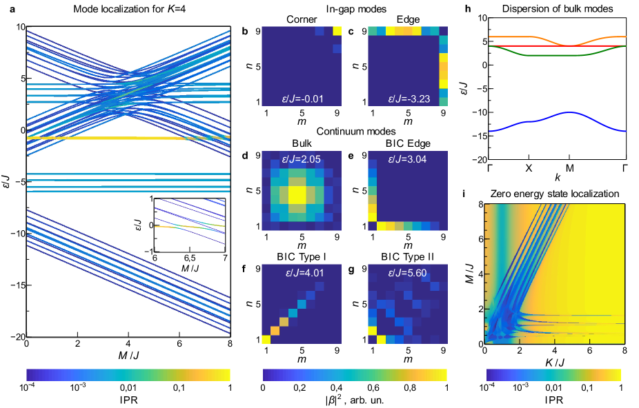
Figure 2: Eigenmodes of the proposed $D_{4}$-symmetric model. a: Energy spectrum of $9\times 9$ structure with coupling constants $J=1$, $K=4$ versus next-nearest-neighbor coupling $M$ in the range $0<M<8$. Color shows the inverse participation ratio (IPR) of the eigenmodes defined by Eq. (2). Inset demonstrates the enlarged fragment of spectrum showing avoided crossings and the formation of hybrid modes upon the interaction of topological corner state with continuum modes. b-c: Eigenmode profiles corresponding to in-gap corner state (b) and edge state (c) at $M=4$. d: delocalized bulk state at $M=4$. e-g: Eigenmode profiles for bound states in the continuum (BIC). e: edge state in the continuum at $M=3.999$. f: BIC Type I corner state at $M=4.007$. g: BIC Type II corner state at $M=5.085$. h: Dispersion diagram for bulk bands of the periodic lattice with couplings $J=1$, $K=M=4$ for the wave vector changing along the $\Gamma-X-M-\Gamma$ trajectory. Different colors correspond to four bulk modes. i: Colorplot for the inverse participation ratio calculated for the state with the energy closest to zero for $9\times 9$ system with $J=1$ as a function of couplings $K$ and $M$.

The eigenstates of both described models [Fig. 1a,c] are found as the solutions to the eigenvalue problem

$$\sum_{m^{\prime},n^{\prime}}H_{mn,m^{\prime}n^{\prime}}\beta_{m^{\prime}n^{\prime}}=\varepsilon\,\beta_{mn}\>,$$ (1)

where $\beta_{mn}$ coefficients describe the amplitude of the field at $(m,n)$ site, $\varepsilon$ is the mode energy defined such that the zero energy corresponds to the resonance frequency of an isolated site, while the Hamiltonian matrix $\hat{H}$ embeds the properties of the system. The nonzero elements of the Hamiltonian $-J$, $-K$, or $-M$ correspond to the coupling links between the respective sites $(m,n)$ and $(m^{\prime},n^{\prime})$ as further discussed in the Methods section. Without loss of generality, we set smaller coupling constant $J=1$, whereas $K>J$.

Solving the eigenvalue problem Eq. (1), we recover the spectra of both systems, without and with next-nearest-neighbor coupling $M$, depicted in Figs. 1b,d, respectively. Regardless of the ratio $K/J$, the canonical two-dimensional (2D) SSH is gapless near the zero energy, and thus the corner state coexists with the continuum of bulk modes [Fig. 1b]. However, diagonal couplings $M$ within each strongly coupled unit cell open a bandgap and yield a spectrally isolated corner-localized state. It should be stressed that the proposed system [Fig. 1c] is the minimal model which captures the effect of long-range interactions in photonic systems since the diagonal links $M$ introduced in the strong coupling unit cell are the dominant terms related to the next-nearest-neighbor interaction. Even though the corner state profile shown in the inset of Fig. 1d strongly resembles that in the canonical quadrupole insulator Benalcazar et al. (2017), all coupling links here are positive, which vastly simplifies the experimental implementation of the proposed system.

To quantify the localization properties of the eigenmodes in our model, we evaluate their inverse participation ratios (IPR) Thouless (1974); Mukherjee and Rechtsman (2020)

$${\rm IPR}=\sum_{n,m}|\beta_{mn}|^{4},$$ (2)

where the summation is performed over all sites $(m,n)$ of the lattice $1\leq m,n\leq N$, and the eigenmode profile is normalized by the condition $\sum_{n,m}|\beta_{mn}|^{2}=1$. There are three scenarios of IPR scaling with the increase of the system size $N$. If the mode is spread over the entire system, the superposition coefficients $\beta_{mn}\propto 1/N$ and hence $IPR\propto 1/N^{2}$. If the eigenstate is confined to the system edge, then $\beta_{mn}\propto 1/\sqrt{N}$, and $IPR\propto 1/N$. Finally, if the mode is localized at the corner, only few $\beta_{mn}$ contribute to the wave function, hence $IPR\approx 1$.

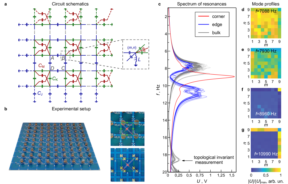
Figure 3: Electric circuit realization. a: Equivalent electric circuit realizing the tight-binding model Fig. 1c. Each node is grounded by the inductor $L$ and connected to its neighbors via capacitors $C_{\rm J}$, $C_{\rm K}$ and $C_{\rm M}$ representing respective tunneling links $J$, $K$ and $M$ of the extended 2D SSH model. The boundary nodes of the circuit are grounded with additional elements to provide the exact mapping between the Kirchhoff’s rules for the circuit and tight-binding equations. Labels $A$, $B$, $C$, and $D$ denote sites of the unit cell in accordance with Fig. 1c. b: The photograph of the experimental $9\times 9$ circuit. Half of the additional diagonal couplings $C_{\rm M}$ are seen at the top side of PCB along with capacitors $C_{\rm J}$, $C_{\rm K}$ and grounding inductors $L$, while the remaining couplings $C_{\rm M}$ are placed at the bottom side carrying also the plugs to connect the measurement equipment. The unit cell of the circuit is shown in the insets to the right. The upper inset demonstrates top view, while the bottom inset shows the opposite side of PCB mirrored to show the matching of the bonds. c: Resonant response of the circuit measured at every node in the range from $1$ to $20$ kHz showing the on-site voltages $U(f)$ between given node $(m,n)$ and ground excited by the external harmonic driving at frequency $f$ with the amplitude $U_{\rm ext}=63$ mV applied between the corresponding node and ground. Grey curves represent bulk and edge nodes with coordinates $1\leq m,n\leq 8$, blue curves correspond to the edge nodes with $1\leq m\leq 8$, $n=9$ and $1\leq n\leq 8$, $m=9$, red curve represents the corner node $m=9$, $n=9$. The arrow points towards the frequency $f=18616$ Hz at which the topological invariant is retrieved. d-g Spatial maps of the on-site voltage responses to the external excitation $U_{\rm ext}=63$ mV at a given frequency $f$ representing bulk (d,e), corner (f), and edge (g) states of the extended SSH model. Color shows the absolute value of voltage between node $(m,n)$ and ground normalized by its maximal value calculated for each map separately.

Thus, increasing the system size, we expect to observe three distinct types of participation ratio scaling. This intuition is confirmed by Fig. 2a, which shows the evolution of the spectrum with the increase of the next-nearest neighbor coupling. Three distinct colors present in the diagram are directly associated with the three types of localization: bright yellow corresponds to the corner state, teal blue color shows the edge states, whereas dark blue depicts bulk states.

The results in Fig. 2a suggest that the corner state is spectrally isolated only for the certain range of next-nearest-neighbor coupling strengths $M_{\rm min}<M<M_{\rm max}$, with $M_{\rm min}\approx 1.6$ and $M_{\rm max}\approx 6.3$ for $K=4$. The corner state profile in such a case is depicted in Fig. 2b featuring a pronounced localization at the corner with the weak coupling links $J$.

The emergence of the corner state in our system is accompanied by the formation of the edge states [Fig. 2c] inherited from the 2D Su-Schrieffer-Heeger model and pinned to the edges terminated by the weak links. Note that the edge states’ energy remains unaffected by the next-nearest-neighbor coupling $M$ as long as the edge states remain confined to the edges where the next-nearest-neighbor coupling is absent [Fig. 2a].

At the same time, the energies of the bulk modes delocalized over the entire 2D system [Fig. 2d] feature a pronounced dependence on $M$. As a result, the bands of bulk and edge states can cross for some parameters interacting with each other and giving rise to more exotic localization types including bound states in the continuum (BIC) Hsu et al. (2016). Interestingly, such BIC states arising in the avoided crossing region of bulk and edge modes can localize at the strong link edges [Fig. 2e] or even at the strong link corner [Fig. 2f,g] in agreement with the prediction of symmetry-protected BIC in the conventional 2D SSH Cerjan et al. (2020). Specifically, the strong link corner hosts two states with different behavior under reflection relative to $m=n$ line: symmetric [Fig. 2f] and antisymmetric [Fig. 2g]. We refer to them as type I and type II BIC corner states, respectively, in analogy to the recent work on photonic kagome lattice Li et al. (2020).

It should be stressed that the BIC Type II corner state appears less localized than BIC Type I. Therefore, for a small $9\times 9$ system considered here, it can be misinterpreted as a bulk excitation. However, analysis of a larger system allows us to prove the localized nature of the mode (Supplementary Note 4).

To probe the topological properties of our model, we examine the bulk bands of a periodic system with a four-site unit cell giving rise to the four bulk bands. While the bulk modes’ dispersion can be derived analytically (Supplementary Note 1), the energies and the field profiles of these modes satisfy generalized chiral symmetry resembling that in kagome lattice Ni et al. (2018). In particular, a sum of eigenvalues corresponding to the four bulk bands of our system is equal to zero [Fig. 2h], and the respective mode profiles are linked to each other via the generalized chiral symmetry operator (see Methods).

Having the energies and the field profiles of the bulk modes, we now assess the topological characteristics of our model by checking the behavior of the field profiles under $C_{2}$ or $C_{4}$ symmetry transformations in few high-symmetry points of the first Brillouin zone Benalcazar et al. (2019). Due to the $C_{4}$ symmetry of the lattice, the topological invariant contains three independent components $\chi=(\#X_{1}^{(2)}-\#\Gamma_{1}^{(2)},\#M_{1}^{(4)}-\#\Gamma_{1}^{(4)},\#M_{2}^{(4)}-\#\Gamma_{2}^{(4)})$, where the upper index denotes the type of the applied rotation operator ($C_{2}$ or $C_{4}$), lower index describes the behavior of the wave function under the symmetry transformation and $\#$ denotes the number of eigenstates with a given transformation law below the particular bandgap in $\Gamma$, $M$ or $X$ point of the first Brillouin zone.

Similar to the SSH model case, the topological invariant depends on the choice of the unit cell. If the unit cell is chosen with the strong links inside, the topological invariant is $(0,0,0)$, indicating the absence of topological states at the strong link corner. However, if the unit cell is chosen with weak links inside [Fig. 1c], the topological invariant appears to be nonzero

$$\chi=(-1,-1,0),$$ (3)

heralding the emergence of higher-order topological corner state with associated corner charge $Q_{\rm corner}=\frac{1}{4}$ and dipole polarization ${\bf P}=(\frac{1}{2},\frac{1}{2})$ Benalcazar et al. (2019). It should be stressed that the topological invariant does not depend on $M$. Nevertheless, next-nearest-neighbor interaction is crucial to open the bandgap at energies close to zero.

Once the topological origin of the corner state is confirmed, we focus on its localization properties. To this end, we trace the evolution of the inverse participation ratio (IPR) of the fixed corner mode in the $9\times 9$ system when the dimerization strength $K/J$ and the next-nearest-neighbor coupling $M/J$ are varied. The calculated phase diagram is shown in Fig. 2i.

We observe that even weak additional couplings $M$ readily yield localized states for certain values of the strong coupling constant $K$. However, the localization deteriorates significantly once the corner mode falls into the continuum of bulk states. Despite the small size of the array, the phase diagram features quite a complicated structure, thus highlighting the rich physics of the proposed model.

To experimentally confirm that the next-nearest-neighbor couplings $M$ provide the crucial ingredient in the formation of in-gap topological corner state, we need to eliminate the contribution of other spurious long-range couplings that inevitably arise in optical or microwave setups based on resonator arrays. To this end, we construct a topological electric circuit, Fig. 3a,b, in which we can directly control the couplings between the sites by placing the desired lumped elements. This extreme flexibility in managing the geometry and amplitudes of the couplings in comparison with the other platforms allows applying electric circuits to emulate such exotic phenomena as four-dimensional quantum Hall phase Wang et al. (2020), two-particle topological states of interacting photons Olekhno et al. (2020), and nonlinearity-induced topological states Hadad et al. (2018) along with the implementation of higher-order topological insulators Imhof et al. (2018); Bao et al. (2019); Liu et al. (2020) and edge states in topological insulators Ningyuan et al. (2015), including the standard two-dimensional SSH model Liu et al. (2019).

The construction of electric circuit model is based upon the exact correspondence between the initial tight-binding problem Eq.(1) describing on-site amplitudes $\beta_{mn}$ and a set of Kirchhoff’s rules describing electric potentials $\varphi_{mn}$ at the respective sites of the equivalent circuit depicted in Fig. 3a. The link between the parameters of the circuit such as capacitances $C_{\rm J}$, $C_{\rm K}$, $C_{\rm M}$, and grounding inductors $L$ from one side and the parameters in the tight-binding model from the other reads:

$$K=\frac{C_{\rm K}}{C_{\rm J}},~{}M=\frac{C_{\rm M}}{C_{\rm J}},~{}\varepsilon=\frac{f_{0}^{2}}{f^{2}}-\left(2+2\frac{C_{K}}{C_{J}}+\frac{C_{M}}{C_{J}}\right)\>,$$ (4)

where $f$ is the frequency of the circuit mode, $\varepsilon$ is the energy in the tight-binding model and $f_{0}=1/(2\pi\,\sqrt{LC_{\rm J}})$ (see Methods for details). Thus, ascending tight-binding energies $\varepsilon$ correspond to the descending mode frequencies $f$ of the electric circuit, which is exploited further.

The experimental realization of the circuit with $C_{\rm J}=1\,\mu{\rm F}$, $C_{\rm K}=C_{\rm M}=4\,\mu{\rm F}$, and $L=23.2\,\mu{\rm H}$ corresponding to the considered model with $K=M=4$ and the size of $9\times 9$ sites is shown in Fig. 3b. Such a circuit has resonances in the kHz frequency range. To probe the modes of the circuit, we apply the external harmonic signal at frequency $f$ with amplitude $U_{\rm ext}=63~{}{\rm mV}$, attaching the signal generator having series impedance $50~{}{\rm Ohm}$ to the given node and ground. Then, we measure the resulting voltage between this node and ground, which characterizes the circuit impedance.

The spectroscopy of the circuit shown in Fig. 3c reveals a bandgap between $9$ and $18$ kHz occupied by the modes in the range $10-12$ kHz localized at the edges of the circuit, and a single mode pinned to the site $(9,9)$ with the frequency around $9$ kHz. Attaching harmonic signal generator to every node of the circuit and measuring the voltages between the given node $(m,n)$ and the ground at a fixed frequency $f$, we recover voltage maps shown in Fig. 3d-g. As seen from these maps, the respective modes represent bulk, edge, and corner states in the considered extended SSH model. The obtained positions of the resonant peaks agree with the results expected from the tight-binding model.

The peaks in the spectrum experience considerable broadening caused by ohmic losses in the inductors and wires of the printed circuit board. Another reason for broadening is the spread in lumped elements’ values, as discussed in Supplementary Note 6. It should be stressed that the in-gap corner state Fig. 3f possesses the largest Q-factor compared to the other resonances in the circuit, reaching $Q\approx 10$. It also remains nearly unperturbed even in the presence of losses and disorder in the component values in contrast to the quasi-BIC corner state Fig. 3e which strongly hybridizes with the bulk states Fig. 3d.

The above robustness is especially interesting since the fluctuations in the values of capacitors in the circuit simultaneously induce off-diagonal and diagonal disorder. Nevertheless, experimental results demonstrate excellent agreement with the theoretical predictions even in the presence of disorder and dissipation for system size as small as $9\times 9$ sites highlighting the potential of higher-order topological states for constructing small-scale photonic and electronic devices. Moreover, we prove the topological origin of the observed corner state, retrieving the topological invariant from the experimental results as described in Supplementary Note 7.

To conclude, we have demonstrated the crucial role played by the next-nearest-neighbor interaction in the formation of higher-order topological states in $D_{4}$-symmetric systems. While the conventional 2D SSH model is gapless at zero energy, even small interaction of the next nearest neighbors opens the topological gap. Thus, our results provide a clear physical interpretation of the corner states observed in recent experiments with the arrays of microwave resonators Xie et al. (2019); Chen et al. (2019). Furthermore, our study reveals the fundamental role of long-range interactions in the formation of higher-order topological phases and highlights the potential of resonant electric circuits to design and test novel topological structures.

Methods

Tight-binding model

To find the dispersion of bulk modes, we construct the Bloch Hamiltonian which is defined in the reciprocal space for a unit cell including four sites and describes bulk excitations in the considered system. For the unit cell choice with intra-cell couplings $J$ shown in Fig. 1c, the Bloch Hamiltonian matrix takes the following form:

$$\hat{H}(k)=-\left(\begin{tabular}[]{c c c c}0&$J+K{\rm e}^{-ik_{\rm x}}$&$M{\rm e}^{ik_{\rm y}-ik_{\rm x}}$&$J+K{\rm e}^{ik_{\rm y}}$\\ $J+K{\rm e}^{ik_{\rm x}}$&0&$J+K{\rm e}^{ik_{\rm y}}$&$M{\rm e}^{ik_{\rm y}+ik_{\rm x}}$\\ $M{\rm e}^{-ik_{\rm y}+ik_{\rm x}}$&$J+K{\rm e}^{-ik_{\rm y}}$&0&$J+K{\rm e}^{ik_{\rm x}}$\\ $J+K{\rm e}^{-ik_{\rm y}}$&$M{\rm e}^{-ik_{\rm y}-ik_{\rm x}}$&$J+K{\rm e}^{-ik_{\rm x}}$&0\end{tabular}\right),$$ (5)

with wave vector components $k_{\rm x}$, $k_{\rm y}$ spanning the range $[-\pi,\pi]$ and directed along the $x$- and $y$-axes shown in Fig. 1. In the above matrix, columns and rows correspond to sites $A$, $B$, $C$, and $D$ left to right and up to down, respectively. Then, we construct a secular equation det$|\hat{H}(k)-\varepsilon\hat{I}|=0$, $\hat{I}$ being the $4\times 4$ unity matrix, which yields four solutions for eigenvalues $\varepsilon(k)$ describing the dispersion of four bulk bands. As shown in Supplementary Note 1, three of these bands are located above zero-energy bandgap, while one band remains below the bandgap. Retrieving the topological invariant from experimental data, we focus on this isolated band. The calculated dispersion diagram is depicted in Fig. 2h.

Topological invariant calculation

To explore the topological properties of our $D_{4}$-symmetric model Fig. 1c, we apply the technique of Ref. Benalcazar et al. (2019) suitable for systems with $C_{n}$ rotational symmetry. To this end, we introduce the matrix of rotation operator by the angle $\pi/2$ that swaps the sites of the unit cell:

$$\hat{R}_{4}=\begin{pmatrix}0\ 1\ 0\ 0\\ 0\ 0\ 1\ 0\\ 0\ 0\ 0\ 1\\ 1\ 0\ 0\ 0\end{pmatrix},$$ (6)

which has the eigenvalues $e^{2\pi i(p-1)/4}$ for $p=1,2,3,4$ describing different behavior of the eigenvector under symmetry transformation. $C_{4}$ symmetry transformation brings $\Gamma$-point with coordinates $(k_{x},k_{y})=(0,0)$ and $M$-point with $(k_{x},k_{y})=(\pi,\pi)$ to the equivalent points of reciprocal space. Hence, as it is straightforward to check, $[\hat{H}(\Gamma),\hat{R}_{4}]=0$ and $[\hat{H}(M),\hat{R}_{4}]=0$. As a result, the eigenstates of the Hamiltonians $\hat{H}(\Gamma)$ and $\hat{H}(M)$ can be enumerated by the index $p$, related to the eigenvalues of $C_{4}$ rotation operator.

Calculating the topological invariant, we also exploit the rotation by the angle $\pi$ described by the operator $\hat{R}_{2}=\hat{R}_{4}^{2}$. This transformation commutes not only with $\hat{H}(\Gamma)$ and $\hat{H}(M)$, but also with $\hat{H}(X)$, where $X$ point of the Brillouin zone has the coordinates $(k_{x},k_{y})=(\pi,0)$. Accordingly, we label the eigenstates of the Hamiltonian $\hat{H}(X)$ by the eigenvalues of $C_{2}$ rotation operator.

The topological invariant is constructed by tracking the number of eigenstates with a certain law of transformation (i.e. fixed index $p$) below the bandgap Benalcazar et al. (2019):

$$\chi^{(4)}\equiv\begin{pmatrix}\#X_{1}^{(2)}-\#\Gamma_{1}^{(2)}\\ \#M_{1}^{(4)}-\#\Gamma_{1}^{(4)}\\ \#M_{2}^{(4)}-\#\Gamma_{2}^{(4)}\end{pmatrix}\>.$$ (7)

Here, the upper indices $(2)$ and $(4)$ correspond to $\hat{R}_{2}$ and $\hat{R}_{4}$ operators, respectively, lower indices denote the value of $p$ for the rotation operator eigenvalues and the symbol $\#$ in front of the high-symmetry point defines the number of eigenfunctions with a given transformation law below the bandgap.

As further discussed in Supplementary Note 2, if the unit cell is chosen with weaker $J$ links inside, the topological invariant is equal to $\chi^{(4)}=(-1,-1,0)$. On the other hand, choosing the unit cell with $K$ and $M$ links inside, we obtain $\tilde{\chi}^{(4)}=(0,0,0)$. These results indicate that the topological corner state arises only at the weak link corner of our system.

Generalized chiral symmetry

The energies and the eigenstates of the four bulk bands are linked to each other via so-called generalized chiral symmetry described by the operator $\hat{\Gamma}_{4}$

$$\Gamma_{4}=\begin{pmatrix}1&0&0&0\\ 0&i&0&0\\ 0&0&-1&0\\ 0&0&0&-i\end{pmatrix}.$$ (8)

Applying this operator to the Bloch Hamiltonian Eq. (5) several times, we obtain a set of matrices:

$$\begin{gathered}\hat{\Gamma}_{4}\hat{H}(k)\hat{\Gamma}_{4}^{-1}=\hat{H}_{\rm 1}(k),\\ \hat{\Gamma}_{4}\hat{H}_{\rm 1}(k)\hat{\Gamma}_{4}^{-1}=\hat{H}_{\rm 2}(k),\\ \hat{\Gamma}_{4}\hat{H}_{\rm 2}(k)\hat{\Gamma}_{4}^{-1}=\hat{H}_{\rm 3}(k),\\ \hat{H}(k)+\hat{H}_{\rm 1}(k)+\hat{H}_{\rm 2}(k)+\hat{H}_{\rm 3}(k)=0,\end{gathered}$$ (9)

By the construction, the traces of all introduced matrices are equal: ${\rm Tr}\{\hat{H}_{\rm 0}\}={\rm Tr}\{\hat{\Gamma}_{4}\hat{H}_{\rm 0}\hat{\Gamma}_{4}^{-1}\}={\rm Tr}\{\hat{H}_{\rm 1}\}={\rm Tr}\{\hat{H}_{\rm 2}\}={\rm Tr}\{\hat{H}_{\rm 3}\}$. On the other hand, since the sum of the matrices is zero, ${\rm Tr}\{\hat{H}+\hat{H}_{\rm 1}+\hat{H}_{\rm 2}+\hat{H}_{\rm 3}\}=0$. Thus, the trace of the Hamiltonian $\hat{H}$ vanishes:

$${\rm Tr}\{\hat{H}\}=0.$$

As a result, the sum of the four eigenvalues of Bloch Hamiltonian for the given $(k_{x},k_{y})$ is equal to zero, which is seen at Fig. 2h, while all eigenstates can be restored from the single eigenstate $\ket{\psi}$ applying generalized chiral symmetry operator: $\ket{\psi_{1}}=\hat{\Gamma}_{4}\,\ket{\psi}$, $\ket{\psi_{2}}=\hat{\Gamma}_{4}\,\ket{\psi_{1}}$ and $\ket{\psi_{3}}=\hat{\Gamma}_{4}\,\ket{\psi_{2}}$.

Electric circuit realization

To construct the electric circuit implementing the proposed model, we start from the explicit form of tight-binding problem Eq.(1), considering bulk node $(m,n)$ labelled with index $B$ in Fig. 1c as an example:

$$-J(\beta_{m-1,n}+\beta_{m,n-1})-K(\beta_{m,n+1}+\beta_{m+1,n})-\\ -M\beta_{m+1,n+1}=\varepsilon\beta_{mn}.$$ (10)

At the same time, potentials and current in the electric circuit are governed by Kirchhoff’s rules $\sum_{m^{\prime},n^{\prime}}I_{m^{\prime}n^{\prime},mn}=0$, stating that the sum of all currents flowing into an arbitrary node $(m,n)$ from all of its neighbors $(m^{\prime},n^{\prime})$ vanishes. The second Kirchhoff’s rule is satisfied automatically by introducing on-site time-dependent potentials $\varphi_{mn}$.

Next, we introduce frequency-dependent complex admittances of the links following the time convention $e^{-i\omega t}$ for varying fields for consistency with Schrödinger equation describing the tight-binding model. With these conventions, the admittances read $\sigma_{C_{\rm J}}(\omega)=-i\omega C_{\rm J}$, $\sigma_{C_{\rm K}}(\omega)=-i\omega C_{\rm K}$, $\sigma_{C_{\rm M}}(\omega)=-i\omega C_{\rm M}$ and $\sigma_{L}(\omega)=-1/(i\omega L)$.

For the corresponding node $(B)$ in the circuit [Fig. 3a] Kirchhoff’s current rule combined with Ohm’s law $I_{m^{\prime}n^{\prime},mn}=\sigma(\omega)(\varphi_{m^{\prime}n^{\prime}}-\varphi_{mn})$ reads $-\sigma_{C_{\rm J}}(\varphi_{m-1,n}+\varphi_{m,n-1})-\sigma_{C_{\rm K}}(\varphi_{m,n+1}+\varphi_{m+1,n})-\sigma_{C_{\rm M}}\varphi_{m+1,n+1}=(-2\sigma_{C_{\rm J}}-2\sigma_{C_{\rm K}}-\sigma_{C_{\rm M}}-\sigma_{C_{\rm J}})\varphi_{mn}$. Dividing the above equation by $\sigma_{C_{\rm J}}$, we obtain

$$-(\varphi_{m-1,n}+\varphi_{m,n-1})-\frac{C_{\rm K}}{C_{\rm J}}(\varphi_{m,n+1}+\varphi_{m+1,n})-\\ -\frac{C_{\rm M}}{C_{\rm J}}\varphi_{m+1,n+1}=\left[\frac{\omega_{0}^{2}}{\omega^{2}}-\left(2+2\frac{C_{K}}{C_{J}}+\frac{C_{M}}{C_{J}}\right)\right]\,\varphi_{mn}\>,$$ (11)

where $\omega_{0}^{2}=1/(L\,C_{J})$. This equation describes on-site potential distributions $\varphi_{mn}$ for the circuit eigenmode with frequency $\omega$ and clearly resembles tight-binding problem Eq. (10). To compensate the absence of neighbors for the boundary nodes maintaining the correspondence between Eq. (10) and Eq. (11), nodes at the sides of the circuit are grounded with additional elements $C_{\rm J}$, $C_{\rm K}$, and $C_{\rm M}$ in parallel to the inductors $L$, in accordance with Fig. 3a. Further details on electric circuit model, including the discussion of the boundary conditions, are provided in Supplementary Note 3.

Experimental setup and measurements

We implement the proposed circuit in the form of a single layer two-sided printed circuit board (PCB) made on the FR4 substrate. The circuit includes $81$ nodes arranged in $9\times 9$ lattice, as shown in Fig. 3a,b. The dimensions of the PCB are $31\times 31$ cm, and the thickness is $2$ mm. Each node of the circuit contains two MCX-type coaxial cable connectors to attach the measurement equipment. The values of circuit elements are $L=(23.19\pm 0.04)\,\mu{\rm H}$, $C_{\rm J}=(931\pm 3)\,{\rm nF}$, and $C_{\rm K}=C_{\rm M}=(4020\pm 10)\,{\rm nF}$. To sort the elements up to the tolerances of $\pm 0.17\%$ for inductors $L$, $\pm 0.32\%$ for capacitors $C_{\rm J}$, and $\pm 0.25\%$ for capacitors $C_{\rm K}$ and $C_{\rm M}$, we use Mastech MS5308 LCR-meter. To characterize resonances in the circuit, we measure the frequency-dependent on-site voltage response between the given circuit node and ground when the external harmonic signal source with amplitude $U_{\rm ext}=63~{}{\rm mV}$ (peak-to-peak voltage $126~{}{\rm mV}$) and series impedance of $50~{}{\rm Ohm}$ is successively attached between every node of the circuit and ground. We study circuit response in the frequency range $f=(1\dots 20)$ kHz, obtaining curves with $1000$ uniformly spaced frequency points. All $81$ voltage curves are shown in Fig. 3c. Such extensive measurements allow us to plot full voltage distributions at the nodes of the circuit in the mentioned frequency range, some of which are shown in Fig. 3d-g. We perform experimental studies with the help of open-source hardware platform OSA103 Mini which includes both the generator and the measurement equipment and allows automating the measurement process. To verify the results, we check the obtained voltage spectra with the help of Keithley $3390$ signal generator and Rohde&Schwarz HMO $2022$ oscilloscope. Further details on the components used and their preparation, as well as on the equipment and measurements, are given in Supplementary Note 5.

Numerical simulations

We perform full numerical simulations of the extended SSH circuit with the help of Keysight Advanced Design System (ADS). Considering the same protocols as in the experimental study, we apply them to a set of circuits with broadly varied parameters of inductors and capacitors, which allows us studying the robustness of circuit resonances towards diagonal and off-diagonal disorder. Besides, we compare the effects of ohmic losses and fluctuations in element values on circuit spectrum and visualize the associated changes in profiles of characteristic resonances. Further details along with simulation results can be found in Supplementary Note 6.

Topological invariant retrieval from experimental data

To fully support our theoretical findings, we extract the topological invariant directly from the experimental measurements of voltage distributions in the circuit. To realize such a procedure, we drive the node $(5,5)$ with a harmonic signal at the amplitude $U_{ext}=50~{}{\rm mV}$ (peak-to-peak voltage $U_{ext}=100~{}{\rm mV}$) in the frequency range $f=1...20~{}{\rm kHz}$ and measure the induced voltage between the given node $(m,n)$ and ground at all nodes of the circuit keeping the external source located at node $(5,5)$ in contrast to spectrum measurements and maps in Fig. 3. Moreover, along with voltage amplitude, we measure relative phases of voltages at all nodes taking the phase of voltage at the node $(5,5)$ as a reference. Performing the procedure outlined in Supplementary Note 7, we extract the approximated Bloch wave function of the bulk state located below the bandgap, analyzing voltage distribution in the circuit at $f=18.616~{}{\rm kHz}$. For the retrieved Bloch wave function, we apply the same procedure as in the theoretical calculation of topological invariant (Supplementary Note 2) and obtain consistent results proving the topological origin of the observed corner state.

Acknowledgments

Theoretical models were supported by the Russian Foundation for Basic Research (grant No. 18-29-20037), experimental studies were supported by the Russian Science Foundation (grant No. 20-72-10065). N.O. and M.G. acknowledge partial support by the Foundation for the Advancement of Theoretical Physics and Mathematics “Basis”.

Author contributions

M.G. and D.Z. conceived the idea. M.G. and N.O supervised the project. V.K., M.G., N.O. and D.Z. developed the theoretical models. N.O. performed numerical studies. A.R. and N.O. carried out circuit simulations. N.O., M.G. and P.S. developed the circuit model. A.D., A.R., O.B. and N.O. fabricated the experimental setup. O.B., A.D. and P.S. performed the experiments. A.R. and N.O. processed the experimental results. N.O. and M.G. prepared the paper with the input from all other authors.

Data availability

The data that support the findings of this study are available from the corresponding authors upon request.

Competing interests

The authors declare that they have no competing interests.

Additional information

Correspondence and requests for materials should be addressed to M.G. (email: m.gorlach@metalab.ifmo.ru) or N.O. (email: nikita.olekhno@metalab.ifmo.ru).

References

- Benalcazar et al. (2017) Wladimir A. Benalcazar, B. Andrei Bernevig, and Taylor L. Hughes, “Quantized electric multipole insulators,” Science 357, 61–66 (2017).
- Schindler et al. (2018a) Frank Schindler, Ashley M. Cook, Maia G. Vergniory, Zhijun Wang, Stuart S. P. Parkin, B. Andrei Bernevig, and Titus Neupert, “Higher-order topological insulators,” Science Advances 4, eaat0346 (2018a).
- Xue et al. (2018) Haoran Xue, Yahui Yang, Fei Gao, Yidong Chong, and Baile Zhang, “Acoustic higher-order topological insulator on a kagome lattice,” Nature Materials 18, 108–112 (2018).
- Ni et al. (2018) Xiang Ni, Matthew Weiner, Andrea Alù, and Alexander B. Khanikaev, “Observation of higher-order topological acoustic states protected by generalized chiral symmetry,” Nature Materials 18, 113–120 (2018).
- Wu and Hu (2015) Long-Hua Wu and Xiao Hu, “Scheme for Achieving a Topological Photonic Crystal by Using Dielectric Material,” Physical Review Letters 114, 223901 (2015).
- Schindler et al. (2018b) Frank Schindler, Zhijun Wang, Maia G. Vergniory, Ashley M. Cook, Anil Murani, Shamashis Sengupta, Alik Yu. Kasumov, Richard Deblock, Sangjun Jeon, Ilya Drozdov, Hélène Bouchiat, Sophie Guéron, Ali Yazdani, B. Andrei Bernevig, and Titus Neupert, “Higher-order topology in bismuth,” Nature Physics 14, 918–924 (2018b).
- Serra-Garcia et al. (2018) Marc Serra-Garcia, Valerio Peri, Roman Süsstrunk, Osama R. Bilal, Tom Larsen, Luis Guillermo Villanueva, and Sebastian D. Huber, “Observation of a phononic quadrupole topological insulator,” Nature 555, 342–345 (2018).
- Mittal et al. (2019) Sunil Mittal, Venkata Vikram Orre, Guanyu Zhu, Maxim A. Gorlach, Alexander Poddubny, and Mohammad Hafezi, “Photonic quadrupole topological phases,” Nature Photonics 13, 692–696 (2019).
- Hassan et al. (2019) Ashraf El Hassan, Flore K. Kunst, Alexander Moritz, Guillermo Andler, Emil J. Bergholtz, and Mohamed Bourennane, “Corner states of light in photonic waveguides,” Nature Photonics 13, 697–700 (2019).
- Peterson et al. (2018) Christopher W. Peterson, Wladimir A. Benalcazar, Taylor L. Hughes, and Gaurav Bahl, “A quantized microwave quadrupole insulator with topologically protected corner states,” Nature 555, 346–350 (2018).
- Li et al. (2020) Mengyao Li, Dmitry Zhirihin, Maxim Gorlach, Xiang Ni, Dmitry Filonov, Alexey Slobozhanyuk, Andrea Alù, and Alexander B. Khanikaev, “Higher-order topological states in photonic kagome crystals with long-range interactions,” Nature Photonics 14, 89–94 (2020).
- Imhof et al. (2018) Stefan Imhof, Christian Berger, Florian Bayer, Johannes Brehm, Laurens W. Molenkamp, Tobias Kiessling, Frank Schindler, Ching Hua Lee, Martin Greiter, Titus Neupert, and Ronny Thomale, “Topolectrical-circuit realization of topological corner modes,” Nature Physics 14, 925–929 (2018).
- Serra-Garcia et al. (2019) Marc Serra-Garcia, Roman Süsstrunk, and Sebastian D. Huber, “Observation of quadrupole transitions and edge mode topology in an LC circuit network,” Physical Review B 99, 020304(R) (2019).
- Bahari et al. (2017) Babak Bahari, Abdoulaye Ndao, Felipe Vallini, Abdelkrim El Amili, Yeshaiahu Fainman, and Boubacar Kanté, “Nonreciprocal lasing in topological cavities of arbitrary geometries,” Science 358, 636–640 (2017).
- Zhang et al. (2020) Weixuan Zhang, Xin Xie, Huiming Hao, Jianchen Dang, Shan Xiao, Shushu Shi, Haiqiao Ni, Zhichuan Niu, Can Wang, Kuijuan Jin, Xiangdong Zhang, and Xiulai Xu, “Low-threshold topological nanolasers based on the second-order corner state,” Light: Science & Applications 9, 109 (2020).
- Han et al. (2020) Changhyun Han, Minsu Kang, and Heonsu Jeon, “Lasing at multidimensional topological states in a two-dimensional photonic crystal structure,” ACS Photonics 7, 2027–2036 (2020).
- Kim et al. (2020) Ha-Reem Kim, Min-Soo Hwang, Daria Smirnova, Kwang-Yong Jeong, Yuri Kivshar, and Hong-Gyu Park, “Multipolar lasing modes from topological corner states,” Nature Communications 11, 5758 (2020).
- Chen et al. (2019) Xiao-Dong Chen, Wei-Min Deng, Fu-Long Shi, Fu-Li Zhao, Min Chen, and Jian-Wen Dong, “Direct observation of corner states in second-order topological photonic crystal slabs,” Physical Review Letters 122, 233902 (2019).
- Xie et al. (2019) Bi-Ye Xie, Guang-Xu Su, Hong-Fei Wang, Hai Su, Xiao-Peng Shen, Peng Zhan, Ming-Hui Lu, Zhen-Lin Wang, and Yan-Feng Chen, “Visualization of higher-order topological insulating phases in two-dimensional dielectric photonic crystals,” Physical Review Letters 122, 233903 (2019).
- Liu and Wakabayashi (2017) Feng Liu and Katsunori Wakabayashi, “Novel topological phase with a zero Berry curvature,” Physical Review Letters 118, 076803 (2017).
- Thouless (1974) David J. Thouless, “Electrons in disordered systems and the theory of localization,” Physics Reports 13, 93–142 (1974).
- Mukherjee and Rechtsman (2020) Sebabrata Mukherjee and Mikael C. Rechtsman, “Observation of Floquet solitons in a topological bandgap,” Science 368, 856–859 (2020).
- Hsu et al. (2016) Chia Wei Hsu, Bo Zhen, A. Douglas Stone, John D. Joannopoulos, and Marin Soljačić, “Bound states in the continuum,” Nature Reviews Materials 1, 16048 (2016).
- Cerjan et al. (2020) Alexander Cerjan, Marius Jürgensen, Wladimir A. Benalcazar, Sebabrata Mukherjee, and Mikael C. Rechtsman, “Observation of a higher-order topological bound state in the continuum,” Physical Review Letters 125, 213901 (2020).
- Benalcazar et al. (2019) Wladimir A. Benalcazar, Tianhe Li, and Taylor L. Hughes, “Quantization of fractional corner charge in -symmetric higher-order topological crystalline insulators,” Physical Review B 99, 245151 (2019).
- Wang et al. (2020) You Wang, Hannah M. Price, Baile Zhang, and Y D. Chong, “Circuit implementation of a four-dimensional topological insulator,” Nature Communications 11, 2356 (2020).
- Olekhno et al. (2020) Nikita A. Olekhno, Egor I. Kretov, Andrei A. Stepanenko, Polina A. Ivanova, Vitaly V. Yaroshenko, Ekaterina M. Puhtina, Dmitry S. Filonov, Barbara Cappello, Ladislau Matekovits, and Maxim A. Gorlach, “Topological edge states of interacting photon pairs emulated in a topolectrical circuit,” Nature Communications 11, 1436 (2020).
- Hadad et al. (2018) Yakir Hadad, Jason C. Soric, Alexander B. Khanikaev, and Andrea Alù, “Self-induced topological protection in nonlinear circuit arrays,” Nature Electronics 1, 178–182 (2018).
- Bao et al. (2019) Jiacheng Bao, Deyuan Zou, Weixuan Zhang, Wenjing He, Houjun Sun, and Xiangdong Zhang, “Topoelectrical circuit octupole insulator with topologically protected corner states,” Physical Review B 100, 201406(R) (2019).
- Liu et al. (2020) Shuo Liu, Shaojie Ma, Qian Zhang, Lei Zhang, Cheng Yang, Oubo You, Wenlong Gao, Yuanjiang Xiang, Tie Jun Cui, and Shuang Zhang, “Octupole corner state in a three-dimensional topological circuit,” Light: Science & Applications 9, 145 (2020).
- Ningyuan et al. (2015) Jia Ningyuan, Clai Owens, Ariel Sommer, David Schuster, and Jonathan Simon, “Time- and site-resolved dynamics in a topological circuit,” Physical Review X 5, 021031 (2015).
- Liu et al. (2019) Shuo Liu, Wenlong Gao, Qian Zhang, Shaojie Ma, Lei Zhang, Changxu Liu, Yuan Jiang Xiang, Tie Jun Cui, and Shuang Zhang, “Topologically protected edge state in two-dimensional Su-Schrieffer-Heeger circuit,” Research 2019, 1–8 (2019).