Reconfigurable Intelligent Surface aided Massive MIMO Systems with Low-Resolution DACs

Abstract

We investigate a reconfigurable intelligent surface (RIS)-aided multi-user massive multiple-input multi-output (MIMO) system where low-resolution digital-analog converters (DACs) are configured at the base station (BS) in order to reduce the cost and power consumption. An approximate analytical expression for the downlink achievable rate is derived based on maximum ratio transmission (MRT) and additive quantization noise model (AQNM), and the rate maximization problem is solved by particle swarm optimization (PSO) method under both continuous phase shifts (CPSs) and discrete phase shifts (DPSs) at the RIS. Simulation results show that the downlink sum achievable rate tends to a constant with the increase of the number of quantization bits of DACs, and four quantization bits are enough to capture a large portion of the performance of the ideal perfect DACs case.

I Introduction

Recently, a reconfigurable intelligent surface (RIS), which can configure the wireless propagation environment, has attracted extensive research interests [1, 2, 3]. Specifically, the RIS is a planar consisting of a large number of passive elements, each of which can manipulate the electromagnetic characteristics of reflected signal independently. By carefully tuning the phase shifts of the RIS, the reflected signals can be constructively added with the direct signals from the BS to enhance the desired signal power, or destructively added with the direct signal to mitigate the undesired signals. Some advantages of RIS-assisted wireless communications include: easy deployment, low hardware cost, enhanced energy- or spectrum-efficiency (EE/SE), and easy integration into the existing networks [4]. As a result, the RIS is expected to push forward an immense influence on improving the transmission performance of future wireless communication networks.

To reap the benefits promised by the RIS, the phase shifts of the reflecting elements at the RIS should be carefully designed. Most of the existing contributions designed the phase shifts based on the instantaneous channel state information (CSI) [5, 6, 7]. This scheme has some drawbacks. Firstly, the phase shifts of the RIS reflecting elements need to be calculated within each channel coherence time that varies rapidly (on the order of milliseconds). This will incur high computational complexity at the base station (BS). Secondly, this scheme requires to estimate instantaneous cascaded CSI that will entail high channel estimation overhead, the amount of which generally increases linearly with the number of reflecting elements. Hence, it is unaffordable for the scenario when the channel coherence time is very short. Thirdly, since the phase shifts need to be updated for each channel coherence time, there will be frequent information exchange between the BS and the RIS. One promising solution to addressing these drawbacks is to design the phase shifts based on the long-term CSI such as angle information [8, 9, 10, 11] or location information [12], which varies much more slowly than instantaneous CSI.

All the above-mentioned contributions [8, 9, 10, 11, 12] assumed the ideally perfect hardware at the BS. Authors in [13] investigated the energy efficiency maximization problem for RIS-aided multi-user communication where the static power of hardware was taken into account. In massive MIMO systems, each antenna is connected to one analog-to-digital converter (ADC) or digital-to-analog converter (DAC), and will consume high power consumption when adopting high-resolution ADC/DACs due to the large number of antennas. Hence, it is appealing to adopt low-resolution ADC/DACs in massive MIMO systems due to its reduced cost and low power consumption [14].

Against the above background, in this paper we study a RIS-aided multi-user massive MIMO system, where the BS is equipped with low-resolution DACs. Specifically, our contributions are summarized as follows:

1. We derive downlink sum achievable rate of the multi-user massive MIMO system based on Rician channel model;

2. We utilize particle swarm optimization (PSO) algorithm to solve the achievable rate maximization problem by optimizing the phase shifts by considering both continuous phase shifts (CPSs) and discrete phase shifts (DPSs);

3. Through simulations, we analyze the impacts of the number of quantization bits of DACs and phase shifts at the RIS on the rate performance, and verify the effectiveness of the proposed algorithm.

Notations: diag$(\mathbf{x})$ denotes a diagonal matrix with the entries of $\mathbf{x}$ on its main diagonal. The symbols $\mathbb{E}\{\cdot\}$, $\textrm{Re}\{\cdot\}$, and $\textrm{Tr}(\cdot)$ denote the expectation operator, real part, and trace, respectively. $\mathbf{I}_{N}$ is the identity matrix with dimension of $N$ . $\mathbb{C}^{M\times N}$ represents the $M\times N$ complex-valued matrix. Besides, $x\sim\mathcal{CN}(a,b)$ denotes that random variable $x$ follows the complex Gaussian distribution with mean $a$ and variance $b$.

II System Model

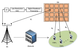
Figure 1: System Model

We consider a downlink multi-user massive MIMO system where a passive RIS with discrete unit elements is deployed to assist the communication from an $M$-antenna BS to $K$ single-antenna mobile users, as shown in Fig. 1. The BS consists of a large-scale uniform linear antenna array (ULA) and each antenna is equipped with a low-resolution DAC, and the RIS is composed of $N$ reflecting elements. We assume that the direct link between the BS and users is neglected due to obstacles, and the RIS is deployed at a proper position where line-of-sight (LoS) communication is ensured for both BS-to-RIS and RIS-to-user links.

Let $\mathbf{G}\in\mathbb{C}^{N\times M}$, $\mathbf{H}=\left[\mathbf{h}_{1},\mathbf{h}_{2},\dots,\mathbf{h}_{K}\right]\in\mathbb{C}^{N\times K}$ respectively denote the channel matrices for the channel between the BS and the RIS, and that between the RIS and $K$ users, and the Rician fading model is adopted for the channel. Here, $\mathbf{h}_{k}^{H}\in\mathbb{C}^{1\times N}$ represents the channel from the RIS to the $k$-th user. Specifically, $\mathbf{G}$ and $\mathbf{h}_{k}^{H}$ can be expressed as:

$$\mathbf{G}=\sqrt{\varepsilon}\left(\sqrt{\frac{K_{G}}{K_{G}+1}}\bar{\mathbf{G}}+\sqrt{\frac{1}{K_{G}+1}}\widetilde{\mathbf{G}}\right)$$ (1)

and

$$\mathbf{h}_{k}^{H}=\sqrt{\beta_{k}}\left(\sqrt{\frac{K_{k}}{K_{k}+1}}{\bf{\bar{h}}}_{k}^{H}+\sqrt{\frac{1}{K_{k}+1}}\tilde{\mathbf{h}}_{k}^{H}\right),$$ (2)

where $\varepsilon$ and $\beta_{k}$ represent the distance-dependent path loss of BS-to-RIS and RIS-to-$k$-th-user paths, and $K_{G}$, $K_{k}$ refer to Rician factors. $\tilde{\mathbf{G}}$, $\tilde{\mathbf{h}}_{k}^{H}$ are scattering components, each element of which is i.i.d. complex Gaussian distributed with zero mean and unit variance and $\bar{\mathbf{G}}$, $\bar{\mathbf{h}}_{k}^{H}$ are LoS components, which can be expressed by the responses of the ULA as:

$$\bar{\mathbf{G}}=\mathbf{a}_{N}\left(\phi_{r}\right)\mathbf{a}_{M}^{H}\left(\phi_{t}\right),\qquad\bar{\mathbf{h}}_{k}^{H}=\mathbf{a}_{N}^{H}\left(\varphi_{kt}\right),$$ (3)

where $\phi_{r}$ is the angle of arrival (AoA) at the RIS, $\phi_{t}$ and $\varphi_{kt}$ are respectively angle of departure (AoD) at the BS and the $k$-th user’s AoD at the RIS. In addition, the array response of an $X$-element ULA is:

$$\mathbf{a}_{X}\left(\vartheta\right)=\left(1,e^{j2\pi\frac{d}{\lambda}\sin\vartheta},\dots,e^{j2\pi\frac{d}{\lambda}\left(X-1\right)\sin\vartheta}\right)^{T},$$ (4)

where $d$ and $\lambda$ are the element spacing and signal wavelength. In this paper, we assume that the statistical CSI can be readily obtained by the existing channel estimation methods.

Define an $N\times N$ diagonal matrix $\mathbf{\Phi}=\textrm{diag}\left(\zeta_{1}\mathbf{e}^{j\theta_{1}},\zeta_{2}\mathbf{e}^{j\theta_{2}},\dots,\zeta_{N}\mathbf{e}^{j\theta_{N}}\right)$ as the reflection coefficient matrix of the RIS, where $\zeta_{n}\in\left[0,1\right]$ and $\theta_{n}\in[0,2\pi)$ for $n=1,2,\dots,N$ represent the amplitude reflection efficiency and the phase shifts induced by the $n$-th reflecting unit, respectively. Without loss of generality, we set $\zeta_{n}=1$ for all $n$.

The unquantized downlink transmission signal at the BS can be written as:

$$\mathbf{x}=\mathbf{W}\mathbf{s},$$ (5)

where $\mathbf{s}=\left(s_{1},s_{2},\dots,s_{K}\right)^{T}\in\mathbb{C}^{K\times 1}$ denotes the transmit signal vector of the BS, which satisfies $\mathbb{E}\left\{\mathbf{s}\mathbf{s}^{H}\right\}=\mathbf{I}_{K}$, and $\mathbf{W}=\left[\mathbf{w}_{1},\mathbf{w}_{2}\dots\mathbf{w}_{K}\right]\in\mathbb{C}^{M\times K}$ denotes the precoding matrix.

Based on additive quantization noise model (AQNM), the downlink transmission signal quantized by DACs at the BS can be expressed as:

$$\mathbf{x}_{q}=Q\left(\mathbf{x}\right)=\alpha\mathbf{x}+\mathbf{n}_{q},$$ (6)

where $Q\left(\cdot\right)$ is a quantization function [15], with $\alpha=1-\rho$, where $\rho$ is the inverse of the signal-to-quantization-noise ratio and $\mathbf{n}_{q}\in\mathbb{C}^{M\times 1}$ denotes the additive Gaussian quantization noise, that is uncorrelated with $\mathbf{x}$, whose covariance is:

$$\mathbf{R}_{\mathbf{n}_{q}\mathbf{n}_{q}}=\mathbb{E}\left\{\mathbf{n}_{q}\mathbf{n}_{q}^{H}\right\}=\alpha\left(1-\alpha\right)\textrm{diag}\left(\mathbf{W}\mathbf{W}^{H}\right).$$ (7)

The values of $\rho$ corresponding to the quantization bits $b$ are listed in Table I for $b\leq 5$ and can be approximated by $\rho=\frac{\sqrt{3}\pi}{2}\cdot 2^{-2b}$ for $b>5$ [14].

TABLE I: $\rho$ VERSUS QUANTIZATION BITS $b$

$b$	1	2	3	4	5
$\rho$	0.3634	0.1175	0.03454	0.009497	0.002499

Therefore, the downlink received signal of the users can be expressed as:

$$\mathbf{y}=\sqrt{P}\mathbf{F}^{H}\mathbf{x}_{q}+\mathbf{n},$$ (8)

where $\mathbf{F}^{H}=\mathbf{H}^{H}\mathbf{\Phi}\mathbf{G}\in\mathbb{C}^{K\times M}$ represents the cascaded BS-RIS-user channel, $P$ represents the transmit power at the BS, and $\mathbf{n}\sim\mathcal{CN}\left(0,\sigma^{2}\mathbf{I}_{K}\right)$ denotes the AWGN vector at the users.

By using (5) and (6), the received signal of the $k$-th user is given by:

$$y_{k}\!=\!\alpha\sqrt{P}\mathbf{f}_{k}^{H}\mathbf{w}_{k}s_{k}+\alpha\textstyle\sum_{i=1,i\neq k}^{K}\!\sqrt{P}\mathbf{f}_{k}^{H}\mathbf{w}_{i}s_{i}\!+\!\sqrt{P}\mathbf{f}_{k}^{H}\mathbf{n}_{q}\!+\!n_{k},$$ (9)

where $\mathbf{f}_{k}^{H}=\mathbf{h}_{k}^{H}\mathbf{\Phi}\mathbf{G}$, with $k=1,2,...,K$. The first term on the right hand side of (9) is the desired signal, the second term is the multi-user interference, the third term is quantization noise and the last term is the AWGN.

III Analysis of Achievable Rate

In this paper, the MRT method is adopted to process the transmit signal at the BS to maximize the signal power gains of the desired users. Then, the precoding matrix $\mathbf{W}$ of the BS is:

$$\mathbf{W}=\frac{\mathbf{F}}{\sqrt{\textrm{Tr}\left(\mathbf{F}^{H}\mathbf{F}\right)}}.$$ (10)

From (9), we can obtain the signal-to-interference-plus-noise ratio (SINR) at the $k$-th user, which can be expressed as:

$$\gamma_{k}={} \frac{\alpha^{2}P\left|\mathbf{f}_{k}^{H}\mathbf{w}_{k}\right|^{2}}{\alpha^{2}P\sum_{i=1,i\neq k}^{K}\left|\mathbf{f}_{k}^{H}\mathbf{f}_{i}\right|^{2}+P\left|\mathbf{f}_{k}^{H}\mathbf{n}_{q}\right|^{2}+|n_{k}|^{2}}$$ (11)

$$={} \frac{\alpha^{2}P\left\|\mathbf{f}_{k}\right\|^{4}}{\alpha^{2}P\sum_{i=1,i\neq k}^{K}\left|\mathbf{f}_{k}^{H}\mathbf{f}_{i}\right|^{2}+P\Gamma|\mathbf{f}_{k}^{H}\mathbf{n}_{q}|^{2}+\Gamma|n_{k}|^{2}},$$

where $\Gamma=\textrm{Tr}\left(\mathbf{F}^{H}\mathbf{F}\right)$. Therefore, the achievable rate of the $k$-th user can be expressed as:

$$R_{k}=\mathbb{E}\left\{\log_{2}{\left(1+\gamma_{k}\right)}\right\}.$$ (12)

A closed-form approximation of (12) is obtained in the following theorem and the sum rate can be written as:

$$R_{\rm{sum}}=\sum_{k=1}^{K}R_{k}.$$ (13)

Theorem 1.

In the RIS-aided massive MIMO System with Low-Resolution DACs, the downlink achievable rate can be approximated as:

$$R_{k}\approx\log_{2}{\left(1+\frac{\alpha^{2}PE_{k}^{signal}}{\alpha^{2}P\sum_{i=1,i\neq k}^{K}I_{ki}+PI_{k}^{DAC}+\sigma^{2}E_{k}^{noise}}\right)},$$ (14)

where $E_{k}^{signal}$, $I_{ki}$, $I_{k}^{DAC}$, and $E_{k}^{noise}$ are respectively given by (15), (16), (17) and (18). Besides, $\delta_{c}=\frac{\varepsilon\beta_{c}}{\left(K_{G}+1\right)\left(K_{c}+1\right)}$, $\psi_{c}(\mathbf{\Phi})=\mathbf{a}_{N}^{H}\left(\phi_{r}\right)\mathbf{\Phi}^{H}\bar{\mathbf{h}}_{c}=\sum_{n=1}^{N}e^{j2\pi\frac{d}{\lambda}(n-1)(\sin(\varphi_{ct})-\sin(\phi_{r}))-j\theta_{n}}\in\mathbb{C}^{1\times 1}$, $c\in\{k,i\}$.

$$E_{k}^{signal}=M\delta_{k}^{2}\times\Big{\{}{M(K_{G}K_{k})^{2}|\psi_{k}(\mathbf{\Phi})|^{4}}+{2K_{G}K_{k}|\psi_{k}(\mathbf{\Phi})|^{2}(2MNK_{G}+MNK_{k}+MN+2M+NK_{k}+N+2)}$$ (15)

$$+{MN^{2}(2K_{G}^{2}+K_{k}^{2}+2K_{G}K_{k}+2K_{G}+2K_{k}+1)}+{N^{2}(K_{G}^{2}+2K_{G}K_{k}+2K_{G}+2K_{k}+1)}$$

$$+MN(2K_{G}+2K_{k}+1)+N(2K_{G}+2K_{k}+1)\Big{\}},$$

$$I_{ki}=M\delta_{k}\delta_{i}\times\Big{\{}{MK_{G}^{2}K_{k}K_{i}|\psi_{k}(\mathbf{\Phi})|^{2}|\psi_{i}(\mathbf{\Phi})|^{2}}+{K_{G}K_{k}|\psi_{k}(\mathbf{\Phi})|^{2}(K_{G}MN+NK_{i}+N+2M)}$$ (16)

$$+{K_{G}K_{i}|\psi_{k}(\mathbf{\Phi})|^{2}(K_{G}MN+NK_{k}+N+2M)}+{N^{2}(MK_{G}^{2}+K_{G}(K_{k}+K_{i}+2)+(K_{k}+1)(K_{i}+1))}$$

$$+{MN(2K_{G}+K_{k}+K_{i}+1)}+{MK_{k}K_{i}\left|\bar{\mathbf{h}}_{k}^{H}\bar{\mathbf{h}}_{i}^{H}\right|^{2}}+{2MK_{G}K_{k}K_{i}\textrm{Re}\left\{\psi_{k}^{H}(\mathbf{\Phi})\psi_{i}(\mathbf{\Phi})\bar{\mathbf{h}}_{i}^{H}\bar{\mathbf{h}}_{k}\right\}}\Big{\}},$$

$$I_{k}^{DAC}=\alpha\left(1-\alpha\right)M\times\Big{\{}\delta^{2}\Big{\{}\left(K_{G}K_{k}\left|\psi_{k}(\mathbf{\Phi})\right|^{2}\right)^{2}\!+\!2N^{2}\left(K_{G}\!+\!K_{k}\!+\!1\right)^{2}\!+\!4K_{G}K_{k}\left|\psi_{k}(\mathbf{\Phi})\right|^{2}\left(N(K_{G}\!+\!K_{k}\!+\!1)+2\right)$$ (17)

$$\!+\!2N(2K_{G}+2K_{k}+1)\Big{\}}+\textstyle\sum_{i=1,i\neq k}^{K}\delta_{k}\delta_{i}\Big{\{}{K_{G}^{2}K_{k}K_{i}|\psi_{k}(\mathbf{\Phi})|^{2}|\psi_{i}(\mathbf{\Phi})|^{2}}+{NK_{G}K_{k}|\psi_{k}(\mathbf{\Phi})|^{2}(K_{G}+K_{i}+1)}$$

$$+{NK_{G}K_{i}|\psi_{i}(\mathbf{\Phi})|^{2}(K_{G}+K_{k}+1)}+{N^{2}(K_{G}^{2}+K_{G}K_{k}+K_{G}K_{i}+K_{k}K_{i}+2K_{G}+K_{k}+K_{i}+1)}\Big{\}}\Big{\}},$$

and

$$E_{k}^{noise}=M\textstyle\sum_{k=1}^{K}\delta_{k}\left(K_{G}K_{k}|\psi_{k}(\mathbf{\Phi})|^{2}+N\left(K_{G}+K_{k}+1\right)\right).$$ (18)

Proof.

By applying [16, Lemma 1] and (7), the achievable rate can be approximated as (19).

$$R_{k}\approx\log_{2}{\left(1+\frac{{\alpha^{2}P\mathbb{E}\left\{\|\mathbf{f}_{k}\|^{4}\right\}}}{{\alpha^{2}P\sum_{i=1,i\neq k}^{K}\mathbb{E}\left\{|\mathbf{f}_{k}^{H}\mathbf{f}_{i}|^{2}\right\}}+{P\mathbb{E}\left\{\Gamma\mathbf{f}_{k}^{H}\mathbf{R}_{\mathbf{n}_{q}\mathbf{n}_{q}}\mathbf{f}_{k}\right\}}+\sigma^{2}\mathbb{E}\left\{\Gamma\right\}}\right)}.$$ (19)

To derive the closed-form expression, we need to derive signal term $\mathbb{E}\left\{\|\mathbf{f}_{k}\|^{4}\right\}$, interference term $\mathbb{E}\left\{|\mathbf{f}_{k}^{H}\mathbf{f}_{i}|^{2}\right\}$, quantization noise term $\mathbb{E}\left\{\Gamma\mathbf{f}_{k}^{H}\mathbf{R}_{\mathbf{n}_{q}\mathbf{n}_{q}}\mathbf{f}_{k}\right\}$ and AWGN noise term $\mathbb{E}\left\{\Gamma\right\}$ after simplification. Define $\mathbf{f}_{km}$ as the $m$-th entry of $\mathbf{f}_{k}$, the first two terms have been given in [10, Lemma 1] and the remaining two terms are derived as :

$$\mathbb{E}\left\{\Gamma\mathbf{f}_{k}^{H}\mathbf{R}_{\mathbf{n}_{q}\mathbf{n}_{q}}\mathbf{f}_{k}\right\}=\alpha\left(1-\alpha\right)\mathbb{E}\left\{\mathbf{f}_{k}^{H}\textrm{diag}\left(\mathbf{F}\mathbf{F}^{H}\right)\mathbf{f}_{k}\right\}$$

$$=\alpha\left(1-\alpha\right)\mathbb{E}\Big{\{}\!\textstyle\sum_{m=1}^{M}\!\left|\mathbf{f}_{km}\right|^{2}\!\Big{(}\!\left|\mathbf{f}_{km}\right|^{2}\!+\!\sum_{i=1,i\neq k}^{K}\!\left|\mathbf{f}_{im}\right|^{2}\!\Big{)}\!\Big{\}}$$

$$=\alpha\left(1-\alpha\right)\Big{(}\textstyle\sum_{m=1}^{M}\mathbb{E}\big{\{}\left|\mathbf{f}_{km}\right|^{4}\big{\}}+\sum_{m=1}^{M}\sum_{i=1,i\neq k}^{K}$$

$$\mathbb{E}\big{\{}\left|\mathbf{f}_{km}\right|^{2}\big{\}}\mathbb{E}\big{\{}\left|\mathbf{f}_{im}\right|^{2}\big{\}}\Big{)},$$ (20)

where

$$\mathbb{E}\big{\{}\left|\mathbf{f}_{km}\right|^{2}\big{\}}=\frac{1}{M}\mathbb{E}\left\{\|\mathbf{f}_{k}\|^{2}\right\}$$ (21)

$$=\delta_{k}\left(K_{G}K_{k}|\psi_{k}(\mathbf{\Phi})|^{2}\!+\!N\left(K_{G}\!+\!K_{k}\!+\!1\right)\right),$$

$$\mathbb{E}\big{\{}\left|\mathbf{f}_{km}\right|^{4}\big{\}}\!=\!\delta^{2}\Big{\{}\left(K_{G}K_{k}\left|\psi_{k}(\mathbf{\Phi})\right|^{2}\right)^{2}\!+\!2N^{2}\left(K_{G}\!+\!K_{k}\!+\!1\right)^{2}$$

$$\!+\!4K_{G}K_{k}\left|\psi_{k}(\mathbf{\Phi})\right|^{2}\left(N(K_{G}\!+\!K_{k}\!+\!1)+2\right)$$ (22)

$$\!+\!2N(2K_{G}+2K_{k}+1)\Big{\}},$$

which can be derived by applying [10, Lemma 1]. In addition, we have

$$\mathbb{E}\left\{\Gamma\right\}\!=\!\mathbb{E}\!\Big{\{}\textstyle\sum_{k=1}^{K}\sum_{m=1}^{M}\left|\mathbf{f}_{km}\right|^{2}\!\Big{\}}\!=\!\sum_{k=1}^{K}\sum_{m=1}^{M}\mathbb{E}\!\left\{\left|\mathbf{f}_{km}\right|^{2}\right\}$$

$$\!=\!M\textstyle\sum_{k=1}^{K}\delta_{k}\left(K_{G}K_{k}|\psi_{k}(\mathbf{\Phi})|^{2}\!+\!N\left(K_{G}\!+\!K_{k}\!+\!1\right)\right).$$ (23)

By substituting (Proof), (Proof) and the useful signal term and interference term into (19), we can obtain the final result. This completes the proof.

IV Phase Shift Optimization

In this section, we aim to maximize the sum achievable rate by optimizing the phase shifts, considering both CPSs and DPSs, based on the long-term CSI, which can be formulated as:

$$\max\limits_{\mathbf{\Phi}}\quad R_{\rm{sum}}$$ (24)

$$\begin{array}[]{r@{\quad}r@{}l@{\quad}l}\rm{s.t.}&\theta_{n}\in{\cal F}_{1}\ \rm{or}\ {\cal F}_{2},\forall n=1,2,...,N.\\ \end{array}$$

where ${{\cal F}_{1}}\!=\!\left\{{\left.{{\theta_{n}}}\right|0\leq{\theta_{n}}\leq 2\pi}\right\}$ and ${{\cal F}_{2}}\!=\!\big{\{}{0,\frac{{2\pi}}{{{2^{B}}}},\cdots,\frac{{2\pi\left({{2^{B}}-1}\right)}}{{{2^{B}}}}}\big{\}}$ denote the sets of continuous and discrete phase shift values, respectively. Here, we limit the period phase in order to simplify the algorithm and $B$ denotes the number of quantization bits of phase shifts at the RIS.

Due to the complex expression of the objective function, we adopt a PSO algorithm in Algorithm 1 owing to its high universality. Supposing the size of particle population is $L$, and the maximum number of iterations is $T$, the complexity of the algorithm is proportional to $L\times T$ [17]. For $i=1,2,\dots,L$, the coordinate position of particle $i$ at time $t$ can be associated to a $1\times N$ phase shift vector ${\bm{\theta}}_{i}^{(t)}=(\theta_{i1},\theta_{i2},\dots,\theta_{iN})$, each element of which is generated randomly limited within ${\cal F}_{1}$ or ${\cal F}_{2}$. Specifically, the difference between ${{\cal F}_{1}}$ and ${{\cal F}_{2}}$ is whether the phase is discretized during initialization.

Algorithm 1 Particle Swarm Optimization Algorithm (PSO)

1:  Particle swarm parameters initialization: Initialize $L$, $T$, $\omega$, $c_{1}$, $c_{2}$, $r_{1}$ ,$r_{2}$;

2:  for $i=1,2,\dots,L$ do

3:     Initialize $\bm{\theta}_{i}^{(0)}$, $\mathbf{v}_{i}^{(0)}$, $\mathbf{p}_{i}^{(0)}=\bm{\theta}_{i}^{(0)}$;

4:  end for

5:  Find $R^{\prime}(\mathbf{p}^{*(0)})=\min\{R^{\prime}(\mathbf{p}_{1}^{(0)}),\dots,R^{\prime}(\mathbf{p}_{L}^{(0)})\}$, and set $\mathbf{g^{(0)}}=\mathbf{p}^{*(0)}$;

6:  while $t\leq T$ do

7:     for  $i=1,2,\dots,L$ do

8:        Update the velocity and position of particles: $\mathbf{v}_{i}^{(t+1)}=\omega\mathbf{v}_{i}^{(t)}+c_{1}r_{1}(\mathbf{p}_{i}-\bm{\theta}_{i}^{(t)})+c_{2}r_{2}(\mathbf{g}-\bm{\theta}_{i}^{(t)})$, $\bm{\theta}_{i}^{(t+1)}=\bm{\theta}_{i}^{(t)}+\mathbf{v}_{i}^{(t+1)}$;

9:        Evaluate fitness value;

10:        Calculate the historical optimal position of particle $i$: $\mathbf{p}_{i}^{(t+1)}=\left\{\begin{array}[]{lc}\mathbf{p}_{i}^{(t)},&R^{\prime}\big{(}\mathbf{p}_{i}^{(t)}\big{)}\leq R^{\prime}\big{(}\bm{\theta}_{i}^{(t+1)}\big{)}\\ \bm{\theta}_{i}^{(t+1)},&R^{\prime}\big{(}\mathbf{p}_{i}^{(t)}\big{)}>R^{\prime}\big{(}\bm{\theta}_{i}^{(t+1)}\big{)}\end{array}\right.$;

11:        Find $R^{\prime}(\mathbf{p}^{*(t+1)})\!=\!\min\{\!R^{\prime}(\mathbf{p}_{1}^{(t+1)}),\!\dots\!,R^{\prime}(\mathbf{p}_{L}^{(t+1)})\!\}$;

12:     end for

13:     Calculate the historical optimal position of the population:$\mathbf{g}^{(t+1)}=\left\{\begin{array}[]{lc}\mathbf{g}^{(t)},&R^{\prime}\left(\mathbf{g}^{(t)}\right)\leq R^{\prime}\big{(}\mathbf{p}^{*(t+1)}\big{)}\\ \mathbf{p}^{*(t+1)},&R^{\prime}\left(\mathbf{g}^{(t)}\right)>R^{\prime}\big{(}\mathbf{p}^{*(t+1)}\big{)}\end{array}\right.$;

14:     Adjust adaptive parameter shown in Algorithm 2;

15:     Set $t\leftarrow t+1$.

16:  end while

The fitness value of each particle is evaluated by using the fitness function $R^{\prime}({\bm{\theta}})$, which can be defined as follows:

$$R^{\prime}({\bm{\theta}})=-R_{\rm{sum}}.\vspace{-0.8ex}$$

Finding the maximum value of $R_{\rm{sum}}$ means finding the minimum value of $R^{\prime}({\bm{\theta}})$, then the minimum value of the reciprocal of the exponential product will be found accordingly.

The velocity of particle $i$ is defined as the distance of particles moving in each iteration, expressed as $\mathbf{v}_{i}^{(t)}=(v_{i1},v_{i2},\dots,v_{iN})$, each of which is limited within $[-v_{\rm{max}},v_{\rm{max}}]$. $\mathbf{p}_{i}^{(t)}$ and $\mathbf{g}^{(t)}$ are respectively defined as the optimal position of particle $i$ and the optimal position of the whole population after $t$ iterations. $\omega$ represents the inertia weight, which is used to adjust the search scope of the solution space and balance the global convergence and convergence rate. $c$, $c_{1}$ and $c_{2}$, and $r_{1}$ and $r_{2}$ respectively represent stagnation counter, acceleration constants, and random values within $[0,1]$.

Algorithm 2 Adjust Adaptive Parameter

1:  Initialize $c=0$;

2:  if  $\mathbf{g}^{(t+1)}<\mathbf{g}^{(t)}$  then

3:     $flag=1$;

4:  else

5:     $flag=0$;

6:  end if

7:  if $flag=0$ then

8:     $c=c+1$;

9:  else

10:     $c=\max\{c-1,0\}$;

11:     if $c<2$ then

12:        $\omega=2\omega$;

13:     else if $c>5$ then

14:        $\omega=\omega/2$;

15:     end if

16:  end if

V Simulation Results

In this section, we evaluate the impact of various parameters on the sum achievable rate performance. Our simulation parameters are set with reference to [7],[10]. We assume the BS and the RIS are placed at $(0,0)$ and $(5,2)$ in a rectangular coordinate system, respectively. The users are uniformly and randomly scattered in a circle centered at $(400,0)$ with radius of 4 m. The AoD of users are randomly generated from $[0,2\pi)$ and these angles will be fixed after initial generation. The large-scale path loss model is modeled in dB as [7]:

$$PL=PL_{0}\left(\frac{D}{D_{0}}\right)^{-\kappa},$$ (25)

where $PL_{0}$ is the path loss at the reference distance $D_{0}$, $D$ is the link length in meters, and $\kappa$ is the path loss exponent. Here, we set the model parmeters as [10]: $D_{0}=1$, $PL_{0}=-30$ dB, the path loss exponents of the BS-to-RIS and RIS-to-$k$-th-user links are $\kappa_{BI}=\kappa_{IU_{k}}=2.8,\forall k$. Unless otherwise stated, our simulation parameters are set as follows: number of users of $K=6$, number of antennas at the BS of $M=64$, number of reflecting elements of the RIS of $N=16$, transmit power of $P=30$ dBm, noise power of $\sigma^{2}=-104$ dBm, Rician factor of $K_{G}=1$, $K_{k}=10,\forall k$. We also set $d=\frac{\lambda}{2}$ in order to mitigate the spatial correlation between antennas. The main parameters for PSO are: $L=\min\{100,10N\}$, $T=200N$, $v_{\rm{max}}=2\pi$, $\omega=0.9$, $c_{1}=c_{2}=1.49$.

Figure 2: The downlink sum achievable rate versus $P$ with $b=1$ under PSO.

It is observed from Fig. 2 that the derived results are consistent with the Monte-Carlo simulation results, which verify the correctness of the derived results. Specifically, we illustrate the downlink sum achievable rates versus transmit power, where one of the curves considers the hardware imbalance, while the other does not and naively regards the actual hardware imbalance as perfect. Specifically, for the conventional naive scheme, we first obtain the beamforming solution under the perfect hardware case, and then substitute the obtained solution into the SINR expression with actual hardware impairment. It is observed from this figure that the proposed algorithm is robust to the hardware impairment.

Fig. 3 shows the downlink sum achievable rate versus the resolution of DACs b. As shown in this figure, the achievable rates increase with b in both cases of CPSs and DPSs. The larger the quantization error, the lower the data rate. Moreover, the rates gradually converge to a constant, which is the achievable rate obtained in the case of $b\to\infty$. It shows that four quantization bits are enough to capture a large portion of the performance of the ideal perfect DACs case.

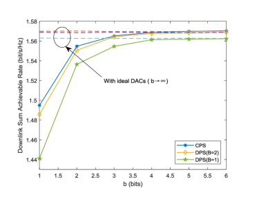
Figure 3: The downlink sum achievable rate versus the number of quantization bits of DACs.

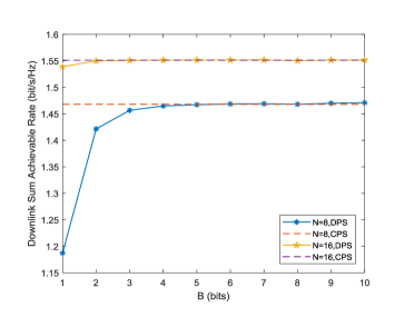
Figure 4: The downlink sum achievable rate versus the number of quantization bits of phase shifts at the RIS.

In fig. 4, we fix $b=1$ and compare the sum achievable rate with the number of quantization bits of phase shifts at the RIS under different $N$. The sum rate increases rapidly when $B$ is small, while the curve gradually saturates when $B$ becomes larger. In addition, when $N$ is large, $B$ has a marginal impact on sum rate.

VI Conclusion

In this paper, a multi-user massive MIMO system aided by a RIS has been discussed, in which each transmit antenna of the BS is equipped with a DAC. The simulation results have proved the correctness of the derived achievable rate and the superiority of using the algorithm when considering low-resolution DACs. A DAC with almost four bits is sufficient to achieve the same rate as an ideal DAC, which verify the rationality of using low-resolution DAC in the system.

References

- [1] C. Huang, S. Hu, G. C. Alexandropoulos, A. Zappone, C. Yuen, R. Zhang, M. D. Renzo, and M. Debbah, “Holographic MIMO surfaces for 6G wireless networks: Opportunities, challenges, and trends,” IEEE Wireless Communications, vol. 27, no. 5, pp. 118–125, 2020.
- [2] M. Renzo, M. Debbah, D. T. Phan-Huy, A. Zappone, M. S. Alouini, C. Yuen, V. Sciancalepore, G. C. Alexandropoulos, J. Hoydis, and H. Gacanin, “Smart radio environments empowered by AI reconfigurable meta-surfaces: An idea whose time has come,” EURASIP Journal on Wireless Communications and Networking, vol. 2019, no. 1, 2019.
- [3] L. Wei, C. Huang, G. C. Alexandropoulos, C. Yuen, Z. Zhang, and M. Debbah, “Channel estimation for RIS-empowered multi-user MISO wireless communications,” IEEE Transactions on Communications, vol. 69, no. 6, pp. 4144–4157, 2021.
- [4] Q. Wu and R. Zhang, “Smart and reconfigurable environment: Intelligent reflecting surface aided wireless network,” IEEE Commun. Mag., vol. 58, no. 1, pp. 106–112, 2020.
- [5] Q. Wu and R. Zhang, “Intelligent reflecting surface enhanced wireless network via joint active and passive beamforming,” IEEE Trans. Wireless Commun., vol. 18, no. 11, pp. 5394–5409, 2019.
- [6] C. Pan, H. Ren, K. Wang, W. Xu, M. Elkashlan, A. Nallanathan, and L. Hanzo, “Multicell MIMO communications relying on intelligent reflecting surfaces,” IEEE Trans. Wireless Commun., vol. 19, no. 8, pp. 5218–5233, 2020.
- [7] C. Pan, H. Ren, K. Wang, M. Elkashlan, A. Nallanathan, J. Wang, and L. Hanzo, “Intelligent reflecting surface aided MIMO broadcasting for simultaneous wireless information and power transfer,” IEEE J. Sel. Areas Commun., vol. 38, no. 8, pp. 1719–1734, 2020.
- [8] Y. Han, W. Tang, S. Jin, C. Wen, and X. Ma, “Large intelligent surface-assisted wireless communication exploiting statistical CSI,” IEEE Trans. Veh. Technol., vol. 68, no. 8, pp. 8238–8242, 2019.
- [9] Z. Peng, T. Li, C. Pan, H. Ren, W. Xu, and M. D. Renzo, “Analysis and optimization for RIS-aided multi-pair communications relying on statistical CSI,” IEEE Transactions on Vehicular Technology, vol. 70, no. 4, pp. 3897–3901, 2021.
- [10] K. Zhi, C. Pan, H. Ren, and K. Wang, “Power scaling law analysis and phase shift optimization of RIS-aided massive MIMO systems with statistical CSI.” [Online]. Available: https://arxiv.org/abs/2010.13525.
- [11] C. Huang, R. Mo, and C. Yuen, “Reconfigurable intelligent surface assisted multiuser MISO systems exploiting deep reinforcement learning,” IEEE Journal on Selected Areas in Communications, vol. 38, no. 8, pp. 1839–1850, 2020.
- [12] X. Hu, C. Zhong, Y. Zhang, X. Chen, and Z. Zhang, “Location information aided multiple intelligent reflecting surface systems,” IEEE Trans. Commun., vol. 68, no. 12, pp. 7948–7962, 2020.
- [13] C. Huang, A. Zappone, G. C. Alexandropoulos, M. Debbah, and C. Yuen, “Reconfigurable intelligent surfaces for energy efficiency in wireless communication,” IEEE Transactions on Wireless Communications, vol. 18, no. 99, pp. 4157–4170, 2019.
- [14] L. Fan, S. Jin, C. Wen, and H. Zhang, “Uplink achievable rate for massive MIMO systems with low-resolution ADC,” IEEE Commun. Lett., vol. 19, no. 12, pp. 2186–2189, 2015.
- [15] Y. Li, C. Tao, A. Lee Swindlehurst, A. Mezghani, and L. Liu, “Downlink achievable rate analysis in massive MIMO systems with one-bit DACs,” IEEE Commun. Lett., vol. 21, no. 7, pp. 1669–1672, 2017.
- [16] Q. Zhang, S. Jin, K. Wong, H. Zhu, and M. Matthaiou, “Power scaling of uplink massive MIMO systems with arbitrary-rank channel means,” IEEE J. Sel. Topics Signal Process., vol. 8, no. 5, pp. 966–981, 2014.
- [17] M. S. Sohail, M. Saeed, S. Z. Rizvi, M. Shoaib, and A. Sheikh, “Low-complexity particle swarm optimization for time-critical applications,” Computer Science, 2014.