A Limit theorem for persistence diagrams of random filtered complexes built over marked point processes

Abstract.

We consider random filtered complexes built over marked point processes on Euclidean spaces. Examples of our filtered complexes include a filtration of $\check{\textrm{C}}$ech complexes of a family of sets with various sizes, growths, and shapes. We establish the law of large numbers for persistence diagrams as the size of the convex window observing a marked point process tends to infinity.

1. Introduction

Much attention has been paid to topological data analysis (TDA) over the last few decades and persistent homology has been playing a central role as one of the most important tools in TDA. Persistent homology measures persistence of topological feature, in particular, appearance and disapperance of homology generators in each dimension and enables us to view data sets in multi-resolutional way. There are several aspects to be discussed in the theory of persistent homology, among which we focus on the random aspect. Data sets to be analyzed are often represented as binomial processes if each data point is regarded as a sample from a certain probability distribution and as stationary point processes if data points are considered as part of a huge object. There have been many works on the topology of binomial processes from the viewpoint of manifold learning [12, 3, 4]. In the setting of stationary point processes, Yogeshwaran-Adler [21] discussed the topology of random complexes built over stationary point processes in the Euclidean space and showed the strong law of large numbers for Betti numbers of such random complexes. In the same setting, Hiraoka-Shirai-Trinh [13] proved the strong law of large numbers for persistence diagrams, which comprise all information about persistence Betti numbers, and also discussed the positivity of its limiting persistence diagram. In the present paper, we extend the framework to deal with random filtered complexes built over stationary marked point processes in order to include more natural examples such as weighted complexes ([2], [6], [15], and references therein).

Given data as a finite point configuration $\Xi$ in ${\mathbb{R}}^{d}$, we consider the union of closed balls $\cup_{x\in\Xi}\overline{B}_{t}(x)$ of radius $t\geq 0$ centered at each data point $x\in\Xi$, which we denoted by $X(\Xi,t)$. We are interested in how the $q$-dimensional homology classes of $X(\Xi,t)$ behave as $t$ grows. By the so-called Nerve theorem, it is well-known that $X(\Xi,t)$ is homotopy equivalent to the $\check{\textrm{C}}$ech complex $C(\Xi,t)$, which is defined as a simplicial complex over points in $\Xi$ consisting of $q$-simplices $\sigma=\{x_{0},x_{1},\dots,x_{q}\}$ for which $\cap_{i=0}^{q}\overline{B}_{t}(x_{i})\neq\emptyset$. We thus obtain a filtration of simplicial complexes $C(\Xi)=\{C(\Xi,t)\}_{t\geq 0}$ from $\Xi$. The $q$th persistent homology of the filtration $C(\Xi)$ gives more topological information of data than the homologies of snapshots of $C(\Xi,t)$ (cf. [10] and [23]).

When we look at an atomic configuration, it is natural to consider the influence of atomic radii. In the usual setting, as explained above, we start from a finite set of points in $\Xi$ and attach balls of radius $t$ to construct the $\check{\textrm{C}}$ech complex, however, taking atomic radii into account, it would be natural to start from a finite set of balls with initial radii rather than a finite set of points. If points are considered to have different shapes, it would be better to attach a different shape of $V_{t}(x_{i})$ to the $i$th point instead of a ball $B_{t}(x_{i})$ depending on the shape of the $i$th point. In many applications, each point often has some extra information and so we would like to incorporate it in our framework. For this purpose, in the present paper, we introduce a filtration of simplicial complexes built over finite sets on ${\mathbb{R}}^{d}$ with marks in a complete separable metric space ${\mathbb{M}}$. Here by marks we mean additional information of data and several information at each point can be expressed as a mark by taking ${\mathbb{M}}$ appropriately.

Now we introduce some notations to state our main theorems. We say that a nonempty finite subset $\Xi$ of ${\mathbb{R}}^{d}\times{\mathbb{M}}$ is a simple marked point set if $\#(\Xi\cap\pi^{-1}\{x\})\leq 1$ holds for any $x\in{\mathbb{R}}^{d}$, where $\#A$ is the cardinality of a set $A$ and $\pi\,:\,{\mathbb{R}}^{d}\times{\mathbb{M}}\to{\mathbb{R}}^{d}$ is the natural projection. For a simple marked point set $\Xi$, by forgetting marks by $\pi$, we obtain a simple point set $\Xi_{g}=\pi(\Xi)\subset{\mathbb{R}}^{d}$ as the ground point set of $\Xi$. For a given simple marked point set $\Xi$, we define a filtration of simplicial complexes ${\mathbb{K}}(\Xi)=\{K(\Xi,t)\}_{t\geq 0}$ with the vertex sets in $\Xi_{g}$ by assigning the birth time $\kappa(\sigma)$ for each simplex $\sigma_{g}=\pi(\sigma)\subset\Xi_{g}$, that is, $K(\Xi,t)=\{\sigma_{g}\subset\Xi_{g}\,:\,\kappa(\sigma)\leq t\}$, where $\kappa$ is a function defined on the nonempty finite subsets of ${\mathbb{R}}^{d}\times{\mathbb{M}}$ with some appropriate conditions (see Section 2.1). We call ${\mathbb{K}}(\Xi)$ the $\kappa$-filtered complex built over a simple marked point set $\Xi$. This is a marked-version of $\kappa$-complex (resp. filtration) introduced in [13] as a generalization of $\check{\textrm{C}}$ech and Vietoris-Rips complex (resp. filtration). For example, if we consider the case where ${\mathbb{M}}$ is the closed interval $[0,R]$ and

$$\kappa(\sigma)=\inf_{w\in{\mathbb{R}}^{d}}\max_{(x,r)\in\sigma}(\|x-w\|-r)^{+}\text{ for finite }\sigma\subset{\mathbb{R}}^{d}\times{\mathbb{M}},$$

then ${\mathbb{K}}(\Xi,t)$ is the $\check{\textrm{C}}$ech complex of the family of closed balls $\{\overline{B}_{t+r}(x)\}_{(x,r)\in\Xi}$, which is the case where we start from balls with various initial radii (Example 2.1). Thus our framework enables us to consider a filtration of $\check{\textrm{C}}$ech complexes of a family of balls with various sizes naturally. Later, we give several examples of $\kappa$-filtered complexes, which include a filtration of $\check{\textrm{C}}$ech complexes of a family of sets with various growth speeds (Example 2.2) and various shapes (Example 2.3). These examples are often called weighted complexes.

For a $\kappa$-filtered complex ${\mathbb{K}}(\Xi)$, its $q$th persistence diagram

$$D_{q}({\mathbb{K}}(\Xi))=\{(b_{i},d_{i})\in\Delta\,:\,i=1,2,\dots,n_{q}\}$$

is defined by a multiset on $\Delta=\{(x,y)\in[0,\infty]\times[0,\infty]\,:\,x<y\}$ determined by the decomposition of the persistent homology (see Section 2.2), which is an expression of the $q$th persistent homology. Each $(b_{i},d_{i})$ means that a $q$th homology class appears at $t=b_{i}$, persists for $b_{i}\leq t<d_{i}$, and disappears at $t=d_{i}$ in ${\mathbb{K}}(\Xi)$. In this paper, the persistence diagram $D_{q}({\mathbb{K}}(\Xi))$ is treated as the counting measure

$$\xi_{q}({\mathbb{K}}(\Xi))=\sum_{(b,d)\in D_{q}({\mathbb{K}}(\Xi))}\delta_{(b,d)},$$

where $\delta_{(x,y)}$ denotes the Dirac measure at $(x,y)\in\Delta$. Let $\Phi$ be a marked point process on ${\mathbb{R}}^{d}$ with marks in ${\mathbb{M}}$. It is a point process on ${\mathbb{R}}^{d}\times{\mathbb{M}}$ such that the ground process $\Phi_{g}(\cdot)=\Phi(\cdot\times{\mathbb{M}})$ is a simple point process on ${\mathbb{R}}^{d}$. We assume that $\Phi_{g}$ has all finite moment, that is, ${\mathbb{E}}[\Phi_{g}(A)^{p}]<+\infty$ for any bounded Borel set $A$ in ${\mathbb{R}}^{d}$ and $p\geq 1$. The restricted marked point process $\Phi$ on $A\times{\mathbb{M}}$ is denoted by $\Phi_{A}$. We discuss the strong law of large numbers for persistence diagrams of a random $\kappa$-filtered complex built over a marked point process, or more precisely, the asymptotic behavior of $\xi_{q}({\mathbb{K}}(\Phi_{A_{n}}))$ ($\xi_{q,A_{n}}$ for short) of the $\kappa$-filtered complex ${\mathbb{K}}(\Phi_{A_{n}})=\{K(\Phi_{A_{n}},t)\}_{t\geq 0}$ as the size of window $A_{n}$ tends to infinity, where $\{A_{n}\}_{n\in{\mathcal{N}}}$ is an increasing net of bounded convex sets in ${\mathbb{R}}^{d}$ with $\sup\{r>0\,:\,A_{n}\text{ contains a ball of radius }r\}\to\infty$ as $n\to\infty$. Such a net is called a convex averaging net in ${\mathbb{R}}^{d}$. The main purpose of this paper is to show the following.

Theorem.

Let $\Phi$ be a stationary ergodic marked point process and suppose its ground process $\Phi_{g}$ has all finite moments. Then for any nonnegative integer $q$, there exists a Radon measure $\nu_{q}$ on $\Delta$ such that for any convex averaging net ${\mathcal{A}}=\{A_{n}\}_{n\in{\mathcal{N}}}$ in ${\mathbb{R}}^{d}$,

$$\frac{1}{\ell(A_{n})}\xi_{q,A_{n}}\xrightarrow{v}\nu_{q}\quad\text{as}\quad n\to\infty\text{ a.s. }$$

where $\ell$ is the $d$-dimensional Lebesgue measure and $\xrightarrow{v}$ denotes the vague convergence of measures on $\Delta$.

New feature of this theorem is two-fold: marks and averaging nets. The same limit theorem above for persistence diagrams is first established in [13, Theorem $1.5$] for the case where $\{A_{n}\}_{n\in{\mathcal{N}}}$ is the rectangles $\{[-L/2,L/2)^{d}\}_{L>0}$ and stationary ergodic point processes (without marks) on ${\mathbb{R}}^{d}$. Marked point processes are often useful from application point of view (cf. [1, 7]) so that this extension greatly expanded the scope of application in TDA. The limit theorem along convex averaging sequences can also be found in a recent article [20] when the underlying filtered complexes are basically $\check{\textrm{C}}$ech complexes. Our theorem is also an extension of [20] to the case of the class of $\kappa$-complexes, which includes $\check{\textrm{C}}$ech complexes as a special example. We also remark that the papers [21] and [22] discuss the limiting behaviour of Betti numbers of random $\check{\textrm{C}}$ech complexes built over stationary point processes.

The paper is organized as follows. We give the statement of our results after introducing some notation and fundamental facts in Section 2. Some examples of marked point processes and $\kappa$-filtered complexes are also presented in this section. In Section 3, we show the law of large numbers for persistent Betti numbers (Theorem 2.7) to prove the main theorem (Theorem 2.6).

2. Preliminaries and the results

2.1. $\kappa$-filtered complexes

For a topological space $S$, let ${\mathcal{F}}(S)$ be the collection of all finite non-empty subsets in $S$. Given a function $f$ on ${\mathcal{F}}(S)$, there exists a permutation invariant function $f_{k}$ on $S^{k}$ such that $f_{k}(s_{1},s_{2},\dots,s_{k})=f(\{s_{1},s_{2},\dots,s_{k}\})$ for any positive integer $k$. We say a function $f$ on ${\mathcal{F}}(S)$ is measurable if the permutation invariant functions $\{f_{k}\}$ are Borel measurable. In this paper, we extend the $\kappa$-filtration for (unmarked) point processes introduced in [13] to that for marked ones. Let ${\mathbb{M}}$ be a complete separable metric space, which stands for the set of marks, and $\kappa\,:\,{\mathcal{F}}({\mathbb{R}}^{d}\times{\mathbb{M}})\to[0,\infty)$ a measurable function satisfying the following:

• $\kappa(A)\leq\kappa(B)$ if $A\subset B$.

• $\kappa$ is invariant under the translations acting on the first component only, i.e.,

  $$\kappa(T_{a}(A))=\kappa(A)$$

  for any $a\in{\mathbb{R}}^{d}$ and for any $A\in{\mathcal{F}}({\mathbb{R}}^{d}\times{\mathbb{M}})$, where $T_{a}\,:(x,m)\mapsto(x+a,m)$.

• There exists an increasing function $\rho\,:\,[0,\infty)\to[0,\infty)$ such that

  $$\|x-y\|\leq\rho(\kappa(\{(x,m),(y,n)\}))$$

  for all $(x,m)$, $(y,n)\in{\mathbb{R}}^{d}\times{\mathbb{M}}$, where $\|\cdot\|$ is the Euclidean norm on ${\mathbb{R}}^{d}$.

Let $\pi\,:\,{\mathbb{R}}^{d}\times{\mathbb{M}}\to{\mathbb{R}}^{d}$ be the projection with respect to the first component. We say $\Xi\in{\mathcal{F}}({\mathbb{R}}^{d}\times{\mathbb{M}})$ is a simple marked point set if for any $x\in{\mathbb{R}}^{d}$, $\#(\Xi\cap\pi^{-1}\{x\})\leq 1$ holds, where $\#A$ is the number of elememts in $A$. For any simple marked point set $\Xi$, we write as $\Xi_{g}=\pi(\Xi)$. The projection $\pi$ naturally induces the bijection

$${\mathcal{F}}(\Xi)\ni\sigma\mapsto\sigma_{g}\in{\mathcal{F}}(\Xi_{g}).$$

Once a simple marked point set $\Xi$ is fixed, each subset $\sigma=\{(x_{0},m_{0}),(x_{1},m_{1}),\dots,(x_{q},m_{q})\}$ of $\Xi$ can be regarded as a finite point configuration $\sigma_{g}=\{x_{0},x_{1},\dots,x_{q}\}$ in ${\mathbb{R}}^{d}$ with marks $\{m_{0},m_{1},\dots,m_{q}\}$ in ${\mathbb{M}}$. By the definition of simple marked point sets we see that each $x\in\Xi_{g}$ has a unique mark $m\in{\mathbb{M}}$ with $(x,m)\in\Xi$.

Given a simple marked point set $\Xi$, we construct a filtration

(2.1) $${\mathbb{K}}(\Xi)=\{K(\Xi,t)\}_{t\geq 0}$$

of simplicial complexes from the simple marked point set $\Xi$ and the function $\kappa$ by

$$K(\Xi,t)=\{\sigma_{g}\subset\Xi_{g}\,:\,\kappa(\sigma)\leq t\},$$

i.e., $\kappa(\sigma)$ is the birth time of a simplex $\sigma_{g}$ in the filtration ${\mathbb{K}}(\Xi)$. Note that whether or not a $q$-simplex $\sigma_{g}=\{x_{0},x_{1},\dots,x_{q}\}\subset\Xi_{g}$ belongs to $K(\Xi,t)$ depends not only on itself but also on the marked set $\sigma=\{(x_{0},m_{0}),(x_{1},m_{1}),\dots,(x_{q},m_{q})\}\subset\Xi$. We call ${\mathbb{K}}(\Xi)=\{K(\Xi,t)\}_{t\geq 0}$ the $\kappa$-filtered complex built over $\Xi$. We also note that the conditions (K1) and (K3) of $\kappa$ yield the following diameter bound

$${\operatorname{diam}\,}\sigma_{g}\leq\rho(t)$$

for any simplex $\sigma\in K(\Xi,t)$. Indeed, for any $\sigma\in K(\Xi,t)$ and any $x,y\in\sigma_{g}$ we take $m,n\in{\mathbb{M}}$ with $(x,m),(y,n)\in\sigma$, then it is easy to see that

$$\|x-y\|\leq\rho(\kappa(\{(x,m),(y,n)\}))\leq\rho(\kappa(\sigma))\leq\rho(t).$$

Example 2.1 ($\check{\textrm{C}}$ech and Vietoris-Rips filtered complex with various sizes).

For a fixed $R>0$, let ${\mathbb{M}}$ be the closed interval $[0,R]$. Fundamental examples of $\kappa$ on ${\mathcal{F}}({\mathbb{R}}^{d}\times{\mathbb{M}})$ are

$$\kappa_{C}(\sigma) =\inf_{w\in{\mathbb{R}}^{d}}\max_{(x,r)\in\sigma}(\|x-w\|-r)^{+}$$

$$\text{and}\quad\kappa_{R}(\sigma) =\max_{(x_{1},r_{1}),(x_{2},r_{2})\in\sigma}\frac{(\|x_{1}-x_{2}\|-r_{1}-r_{2})^{+}}{2},$$

where $a^{+}=\max\{a,0\}$ for $a\in{\mathbb{R}}$. It is easy to see that they satisfy (K1), (K2), and (K3) with $\rho(t)=2t+2R$. We denote the corresponding $\kappa$-filtered complexes built over a simple marked point set $\Xi$ by ${\mathbb{C}}(\Xi)=\{C(\Xi,t)\}_{t\geq 0}$ and ${\mathbb{R}}(\Xi)=\{R(\Xi,t)\}_{t\geq 0}$ respectively. For $\sigma\in{\mathcal{F}}(\Xi)$, we see that

$$\kappa_{C}(\sigma)\leq t \Leftrightarrow\bigcap_{(x,r)\in\sigma}\overline{B}_{t+r}(x)\neq\emptyset,$$

$$\kappa_{R}(\sigma)\leq t \Leftrightarrow\overline{B}_{t+r_{1}}(x_{1})\cap\overline{B}_{t+r_{2}}(x_{2})\neq\emptyset\quad\text{ for any }(x_{1},r_{1}),(x_{2},r_{2})\in\sigma,$$

where $\overline{B}_{r}(x)=\{y\in{\mathbb{R}}^{d}\,:\,\|y-x\|\leq r\}$ is the closure of the open ball $B_{r}(x)$ of radius $r$ centered at $x$. Hence $C(\Xi,t)$ and $R(\Xi,t)$ are the so-called $\check{\textrm{C}}$ech complex and Vietoris-Rips complex of the family of balls $\{\overline{B}_{t+r}(x)\}_{(x,r)\in\Xi}$.

Example 2.2 ($\check{\textrm{C}}$ech and Vietoris-Rips filtered complex with various growth speeds).

Let ${\mathbb{M}}$ be a finite family $\{\bm{r}_{i}(\cdot)\}_{i\in I}$ of right continuous, strictly increasing functions on $[0,\infty)$. We define functions on ${\mathcal{F}}({\mathbb{R}}^{d}\times{\mathbb{M}})$ by

$$\kappa_{C}(\sigma) =\inf_{w\in{\mathbb{R}}^{d}}\max_{(x,\bm{r})\in\sigma}\bm{r}^{-1}(\|x-w\|)$$

$$\text{ and }\quad\kappa_{R}(\sigma) =\max_{(x_{1},\bm{r}_{1}),(x_{2},\bm{r}_{2})\in\sigma}(\bm{r}_{1}+\bm{r}_{2})^{-1}(\|x_{1}-x_{2}\|),$$

where $\bm{r}^{-1}(t)=\inf\{s\geq 0\,:\,\bm{r}(s)\geq t\}$. One can show that

$$\kappa_{C}(\sigma)\leq t \Leftrightarrow\bigcap_{(x,\bm{r})\in\sigma}\overline{B}_{\bm{r}(t)}(x)\neq\emptyset,$$

$$\kappa_{R}(\sigma)\leq t \Leftrightarrow\overline{B}_{\bm{r}_{1}(t)}(x_{1})\cap\overline{B}_{\bm{r}_{2}(t)}(x_{2})\neq\emptyset\text{ for any }(x_{1},\bm{r}_{1}),(x_{2},\bm{r}_{2})\in\sigma$$

in the same way as Example 2.1 above. In this case, (K3) is satisfied with $\rho(t)=2\max_{i\in I}\bm{r}_{i}(t)$. The corresponding $\kappa$-filtered complexes are the $\check{\textrm{C}}$ech complexes and Vietoris-Rips complexes of the family of balls $\{\overline{B}_{\bm{r}(t)}(x)\}_{(x,\bm{r})\in\Xi}$ for a simple marked point set $\Xi\in{\mathcal{F}}({\mathbb{R}}^{d}\times{\mathbb{M}})$.

Example 2.3 ($\check{\textrm{C}}$ech filtered complex with various shapes).

Let ${\mathbb{M}}$ be a finite family $\{C_{i}\}_{i\in I}$ of bounded convex sets in ${\mathbb{R}}^{d}$ satisfying that $0\in{\operatorname{int}\,}C_{i}$ for every $i\in I$, where ${\operatorname{int}\,}C$ is the interior of $C$. We put $f_{C}(z)=\inf\{s\geq 0\,:\,z\in sC\}$ for a convex set $C$ and $z\in{\mathbb{R}}^{d}$. Consider the function on ${\mathcal{F}}({\mathbb{R}}^{d}\times{\mathbb{M}})$ defined by

$$\kappa(\sigma)=\inf_{w\in{\mathbb{R}}^{d}}\max_{(x,C)\in\sigma}f_{C}(w-x).$$

This satisfies (K3) with $\rho(t)=2t\max_{i\in I}{\operatorname{diam}\,}C_{i}$. For any simple marked point set $\Xi\in{\mathcal{F}}({\mathbb{R}}^{d}\times{\mathbb{M}})$, it is easy to see that the corresponding $K(\Xi,t)$ is the $\check{\textrm{C}}$ech complex of the family of sets $\{t\overline{C}+x\}_{(x,C)\in\Xi}$.

2.2. Persistent homologies and persistence diagrams

In what follows, we fix a function $\kappa$ satisfying the conditions (K1)–(K3) in Section 2.1. Now we give a brief introduction of persistent homology, persistence diagrams, and persistent Betti numbers for the $\kappa$-filtered complex ${\mathbb{K}}(\Xi)$. Let ${\mathbb{F}}$ be a field. Given a nonnegative integer $q$ and $t\geq 0$, we denote by $H_{q}(K(\Xi,t))$ the $q$th homology group of the simplicial complex $K(\Xi,t)$ with coefficients in ${\mathbb{F}}$. For $r\leq s$, the inclusion $K(\Xi,r)\hookrightarrow K(\Xi,s)$ induces the linear map $\iota_{r}^{s}\,:\,H_{q}(K(\Xi,r))\to H_{q}(K(\Xi,s))$. We put $H_{q}({\mathbb{K}}(\Xi))=(H_{q}(\{{\mathbb{K}}(\Xi,t)\}_{t\geq 0},\{\iota_{r}^{s}\}_{s\geq r\geq 0})$ and call it the $q$th persistent homology (or persistence module) of $K(\Xi)$. It is well-known that there exist a unique nonnegative integer $n_{q}$ and $b_{i},d_{i}\in[0,\infty]$ with $b_{i}<d_{i}$, $i=1,2,\dots,n_{q}$, such that the $q$th persistent homology $H_{q}({\mathbb{K}}(\Xi))$ has a decomposition property

(2.2) $$H_{q}({\mathbb{K}}(\Xi))\simeq\bigoplus_{i=1}^{n_{q}}I(b_{i},d_{i}),$$

where $I(b_{i},d_{i})=(U_{r},f_{r}^{s})$ consists of a family of vector spaces

$$U_{r}=\begin{cases}{\mathbb{F}}\quad&b_{i}\leq r<d_{i},\\ 0\quad&\text{ otherwise, }\end{cases}$$

and the identity map $f_{r}^{s}={\operatorname{id}}_{{\mathbb{F}}}$ for $b_{i}\leq r\leq s<d_{i}$. Each $I(b_{i},d_{i})$ in (2.2) describes that a topological feature ($q$th homology class) appears at $t=b_{i}$, persists for $b_{i}\leq t<d_{i}$, and disappears at $t=d_{i}$ in ${\mathbb{K}}(\Xi)$. We call the pair $(b_{i},d_{i})$ its birth-death pair. The $q$th persistence diagram of ${\mathbb{K}}(\Xi)$ is defined by a multiset

$$D_{q}({\mathbb{K}}(\Xi))=\{(b_{i},d_{i})\in\Delta\,:\,i=1,2,\dots,n_{q}\},$$

where $\Delta=\{(x,y)\in[0,\infty]\times[0,\infty]\,:\,x<y\}$. Let $m_{b,d}$ be the multiplicity of the point $(b,d)\in D_{q}(\Xi)$ and $\xi_{q}({\mathbb{K}}(\Xi))$ the counting measure on $\Delta$ given by

$$\xi_{q}({\mathbb{K}}(\Xi))=\sum_{(b,d)}m_{b,d}\delta_{(b,d)},$$

where $\delta_{(x,y)}$ is the Dirac measure at $(x,y)\in\Delta$. We identify the persistence diagram $D_{q}({\mathbb{K}}(\Xi))$ with the counting measure $\xi_{q}({\mathbb{K}}(\Xi))$. The $q$th $(r,s)$-persistent Betti number is also defined by

$$\beta_{q}^{r,s}({\mathbb{K}}(\Xi))=\dim\frac{Z_{q}(K(\Xi,r))}{Z_{q}(K(\Xi,r))\cap B_{q}(K(\Xi,s))},$$

where $Z_{q}(K(\Xi,r))$ and $B_{q}(K(\Xi,r))$ are the $q$th cycle group and boundary group of $K(\Xi,r)$, respectively. It is easy to see that this number is equal to the rank of $\iota_{r}^{s}\,:\,H_{q}(K(\Xi,r))\to H_{q}(K(\Xi,s))$. By definition of the persistent Betti number, we have

(2.3) $$\beta_{q}^{r,s}({\mathbb{K}}(\Xi))=\sum_{b\leq r,s<d}m_{b,d}=\xi_{q}({\mathbb{K}}(\Xi))([0,r]\times(s,\infty]).$$

Therefore the persistence Betti number $\beta_{q}^{r,s}$ counts the number of birth-death pairs in the persistence diagram $D_{q}({\mathbb{K}}(\Xi))$ located in the gray region of Figure 1.

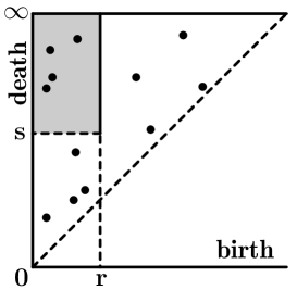
Figure 1. $\beta_{q}^{r,s}$ counts the number of birth-death pairs in the gray region.

Details for these facts can be found in [10], [13] and [23] for example.

2.3. Marked point processes

Now we consider marked point processes. Let $X$ be a complete separable metric space and ${\mathcal{B}}(X)$ the Borel $\sigma$-field on $X$. A Borel measure $\mu$ on $X$ is boundedly finite if $\mu(A)<\infty$ for every bounded Borel set $A$. We say that a sequence $\{\mu_{n}\}$ of boundedly finite measures on $X$ converges to a boundedly finite measure $\mu$ on $X$ in the $w^{\#}$-topology if

(2.4) $$\int_{X}f\,d\mu_{n}\to\int_{X}f\,d\mu\text{ as }n\to\infty$$

for all bounded continuous functions $f$ on $X$ vanishing outside a bounded set. We denote by ${\mathcal{M}}_{X}^{\#}$ the totality of boundedly finite measures on ${\mathcal{B}}(X)$. ${\mathcal{M}}_{X}^{\#}$ is a complete separable metric space under the $w^{\#}$-topology. The corresponding $\sigma$-field ${\mathcal{B}}({\mathcal{M}}_{X}^{\#})$ coincides with the smallest $\sigma$-field with respect to which the mappings $\mu\mapsto\mu(A)$ are measurable for all $A\in{\mathcal{B}}(X)$. If $X$ is a locally compact Hausdorff space with countable base, we can take a metric so that $X$ is complete and every bounded subset of $X$ is relatively compact. Then a Borel measure is boundedly finite if and only if it is a Radon measure and $w^{\#}$-convergence coincides with vague convergence. We recall that a Radon measure is a measure on $X$ taking finite values on compact sets and a sequence $\{\mu_{n}\}$ of Radon measures on $X$ converges to a Radon measure $\mu$ on $X$ vaguely (or in the vague topology) if $(\ref{def:weak hash})$ holds for each continuous function $f$ on $X$ vanishing outside a compact set. In this case, we write $\mu_{n}\xrightarrow{v}\mu$. Let ${\mathcal{N}}_{X}^{\#}$ be the totality of boundedly finite integer-valued measures. We call a measure in ${\mathcal{N}}_{X}^{\#}$ a counting measure for short. For a counting measure $\mu$ on $X$, there exist sequences of positive integers $\{k_{i}\}$ and points $\{x_{i}\}$ in $X$ with at most finitely many $x_{i}$ in any bounded Borel set such that

$$\mu=\sum_{i}k_{i}\delta_{x_{i}}.$$

Note that ${\mathcal{N}}_{X}^{\#}$ is a closed subset of ${\mathcal{M}}_{X}^{\#}$.

Let $(\Omega,{\mathcal{F}},{\mathbb{P}})$ be a probability space. An $({\mathcal{M}}_{X}^{\#},{\mathcal{B}}({\mathcal{M}}_{X}^{\#}))$ (resp., $({\mathcal{N}}_{X}^{\#},{\mathcal{B}}({\mathcal{N}}_{X}^{\#}))$-valued random variable $\xi$ on $(\Omega,{\mathcal{F}},{\mathbb{P}})$ is called a random measure (resp., point process) on $X$. A point process $\xi$ is typically identified with the random point configuration of its atoms. The expectation measure (or mean measure) of $\xi$ is defined so that $M(A)={\mathbb{E}}[\xi(A)]$ for any $A\in{\mathcal{B}}(X)$. It is often denoted by ${\mathbb{E}}[\xi]$. We say that a point process $\xi$ is simple if

$${\mathbb{P}}(\xi(\{x\})=0\text{ or }1\text{ for any }x\in X)=1.$$

A marked point process on ${\mathbb{R}}^{d}$ with marks in ${\mathbb{M}}$ is a point process $\Phi$ on ${\mathbb{R}}^{d}\times{\mathbb{M}}$ whose marginal point process $\Phi_{g}(\cdot)=\Phi(\cdot\times{\mathbb{M}})$ on ${\mathbb{R}}^{d}$ is a simple point process on ${\mathbb{R}}^{d}$. The point process $\Phi_{g}$ is called the ground process of $\Phi$. We say that the ground process $\Phi_{g}$ has all finite moments if ${\mathbb{E}}[\Phi_{g}(A)^{p}]<+\infty$ for every bounded $A\in{\mathcal{B}}({\mathbb{R}}^{d})$ and every $p\geq 1$. The translations $\{T_{a}\}_{a\in{\mathbb{R}}^{d}}$ on ${\mathbb{R}}^{d}\times{\mathbb{M}}$ induce the translations $\{{T_{a}}_{\ast}\}_{a\in{\mathbb{R}}^{d}}$ on ${\mathcal{N}}_{{\mathbb{R}}^{d}\times{\mathbb{M}}}^{\#}$ defined by

$$({T_{a}}_{\ast}\mu)(A)=\mu(T_{a}^{-1}A)$$

for $a\in{\mathbb{R}}^{d}$ and $A\in{\mathcal{B}}({\mathbb{R}}^{d}\times{\mathbb{M}})$. A marked point process is called stationary if its probability distribution is translation invariant. A stationary marked point process $\Phi$ is called ergodic if the only members $B$ of ${\mathcal{B}}({\mathcal{N}}_{{\mathbb{R}}^{d}\times{\mathbb{M}}}^{\#})$ with ${\mathbb{P}}\circ\Phi^{-1}({T_{a}}_{\ast}B\Delta B)=0$ for all $a\in{\mathbb{R}}^{d}$ satisfy ${\mathbb{P}}\circ\Phi^{-1}(B)=0\text{ or }1$.

Example 2.4 (point process with i.i.d. marks).

Let $\Phi_{g}$ be a point process on ${\mathbb{R}}^{d}$ and $\{X_{i}\}$ a measurable enumeration of $\Phi_{g}$, that is, $\{X_{i}\}$ is a sequence of ${\mathbb{R}}^{d}$-valued random variables so that $\Phi_{g}=\sum_{i}\delta_{X_{i}}$ a.s. We take an i.i.d. sequence of ${\mathbb{M}}$-valued random variables $\{M_{i}\}$ such that $\Phi=\{X_{i}\}$ and $\{M_{i}\}$ are independent. A marked point process on ${\mathbb{R}}^{d}$ with marks in ${\mathbb{M}}$ is defined by

$$\Phi=\sum_{i}\delta_{(X_{i},M_{i})}.$$

If the point process $\Phi$ is stationary (and ergodic), then so is $\Phi$.

Example 2.5.

Let $\Phi_{g}$ be a simple stationary (ergodic) point process on ${\mathbb{R}}^{d}$ and $\{X_{i}\}$ a measurable enumeration of $\Phi_{g}$. For a fixed $R>0$ and for each $i$, we define a $\{0,1\}$-valued random variable $M_{i}$ by

(2.5) $$M_{i}=\begin{cases}1,&\text{ if there exists }j\neq i\text{ such that }|X_{i}-X_{j}|\leq R,\\ 0,&\text{ otherwise. }\end{cases}$$

The point process on ${\mathbb{R}}^{d}\times\{0,1\}$ defined by

$$\Phi=\sum_{i}\delta_{(X_{i},M_{i})}$$

is a marked point process. In general, for measurable maps $M_{i}\colon{\mathcal{N}}_{{\mathbb{R}}^{d}}^{\#}\to{\mathbb{M}}\,(i\geq 1)$, the point process on ${\mathbb{R}}^{d}\times{\mathbb{M}}$ defined by

$$\Phi=\sum_{i}\delta_{(X_{i},M_{i}(\Phi_{g}))}$$

is a stationary marked point process.

Incidentally, for $M_{i}\,(i\geq 1)$ in (2.5), the point process

$$\Phi_{I}=\sum_{i:M_{i}=0}\delta_{X_{i}}$$

on ${\mathbb{R}}^{d}$ is called a Matérn type I construction of $\Phi$ (See [16]).

Other examples and basic facts for marked point processes are available in [8] and [9].

2.4. Main theorems

In order to state the main results we introduce the notion of convex averaging nets in ${\mathbb{R}}^{d}$. Let $({\mathcal{N}},\leq)$ be a linearly ordered set. A family ${\mathcal{A}}=\{A_{n}\}_{n\in{\mathcal{N}}}$ of bounded Borel sets in ${\mathbb{R}}^{d}$ is a convex averaging net if

• $A_{n}$ is convex for each $n\in{\mathcal{N}}$,

• $A_{n}\subset A_{m}$ for $n\leq m$, and

• $\displaystyle{\sup_{n\in{\mathcal{N}}}r(A_{n})=\infty}$, where $r(A)=\sup\{r>0\,:\,A\text{ contains a ball of radius }r\}$.

Given a marked point process $\Phi$ and $A\in{\mathcal{B}}({\mathbb{R}}^{d})$, we denote the restricted marked point process $\Phi$ on $A\times{\mathbb{M}}$ by $\Phi_{A}$, i.e., $\Phi_{A}(\cdot)=\Phi(\cdot\cap(A\times{\mathbb{M}}))$. Note that $\Phi_{A}$ can be regarded as a random simple marked point set for any bounded $A$. For any convex averaging net ${\mathcal{A}}=\{A_{n}\}_{n\in{\mathcal{N}}}$, a random $\kappa$-filtered complex with parameter $n\in{\mathcal{N}}$ is defined by ${\mathbb{K}}(\Phi_{A_{n}})=\{K(\Phi_{A_{n}},t)\}_{t\geq 0}$. For the sake of simplicity, we often denote the corresponding $q$th persistence diagram $\xi_{q}({\mathbb{K}}(\Phi_{A_{n}}))$ and $q$th $(r,s)$-persistent Betti number $\beta_{q}^{r,s}({\mathbb{K}}(\Phi_{A_{n}}))$ by $\xi_{q,A_{n}}$ and $\beta_{q,A_{n}}^{r,s}$ respectively.

Now we are in a position to state the main theorem.

Theorem 2.6.

Let $\Phi$ be a stationary marked point process and suppose its ground process $\Phi_{g}$ has all finite moments. Then for any nonnegative integer $q$, there exists a Radon measure $\nu_{q}$ on $\Delta$ such that for any convex averaging net ${\mathcal{A}}=\{A_{n}\}_{n\in{\mathcal{N}}}$ in ${\mathbb{R}}^{d}$,

$$\frac{1}{\ell(A_{n})}{\mathbb{E}}[\xi_{q,A_{n}}]\xrightarrow{v}\nu_{q}\quad\text{as}\quad n\to\infty,$$

where $\ell$ is the $d$-dimensional Lebesgue measure. Furthermore if $\Phi$ is ergodic, then

$$\frac{1}{\ell(A_{n})}\xi_{q,A_{n}}\xrightarrow{v}\nu_{q}\quad\text{as}\quad n\to\infty\text{ a.s. }$$

Theorem 2.6 can be proved by a general theory of Radon measures for the vague convergence and the following law of large numbers for persistent Betti numbers.

Theorem 2.7.

Let $\Phi$ be a stationary marked point process and suppose its ground process $\Phi_{g}$ has all finite moments. Then, for any $0\leq r\leq s<\infty$ and nonnegative integer $q$, there exists a nonnegative number $\hat{\beta}_{q}^{r,s}$ such that for any convex averaging net ${\mathcal{A}}=\{A_{n}\}_{n\in{\mathcal{N}}}$ in ${\mathbb{R}}^{d}$,

$$\frac{1}{\ell(A_{n})}{\mathbb{E}}[\beta_{q,A_{n}}^{r,s}]\to\hat{\beta}_{q}^{r,s}\qquad\text{as}\quad n\to\infty.$$

Furthermore, if $\Phi$ is ergodic, then

$$\frac{1}{\ell(A_{n})}\beta_{q,A_{n}}^{r,s}\to\hat{\beta}_{q}^{r,s}\quad\text{ as }\quad n\to\infty\text{ a.s. }$$

The proofs of Theorem 2.6 and Theorem 2.7 will be given in the next Section. They are shown in the same way as [13, Theorem $1.5$ and Theorem $1.11$], in which such limit theorems for stationary (unmarked) point processes were proved.

3. Proof of Theorems 2.6 and 2.7

The aim of this section is to prove Theorem 2.6 and Theorem 2.7.

3.1. Convergence of persistent Betti numbers

Let $M,h$ be positive numbers and $A\in{\mathcal{B}}({\mathbb{R}}^{d})$. We put

$$\Lambda_{M} =[-M/2,M/2)^{d},$$

$$\underline{A}^{(M)} =\bigsqcup\{\Lambda_{M}+z\,:\,z\in M{\mathbb{Z}}^{d}\text{ and }(\Lambda_{M}+z)\subset A\},$$

$$\overline{A}^{(M)} =\bigsqcup\{\Lambda_{M}+z\,:\,z\in M{\mathbb{Z}}^{d}\text{ and }(\Lambda_{M}+z)\cap A\neq\emptyset\},$$

$$\text{ and }\partial A^{h} =\{x\in{\mathbb{R}}^{d}\,:\,d(x,\partial A)\leq h\},$$

where $M{\mathbb{Z}}^{d}=\{Mz\,:\,z\in{\mathbb{Z}}^{d}\}$ and $\displaystyle{d(x,\partial A)=\inf_{y\in\partial A}|x-y|}$. Fundamental results treated in this paper for convex averaging nets are summarized in the next proposition.

Proposition 3.1.

Let ${\mathcal{A}}=\{A_{n}\}_{n\in{\mathcal{N}}}$ be a convex averaging net in ${\mathbb{R}}^{d}$. Then for any $M>0$ and $h>0$, as $n\to\infty$,

(3.1) $$\frac{\ell(\underline{A}_{n}^{(M)})}{\ell(A_{n})}\to 1,\quad\frac{\ell(\overline{A}_{n}^{(M)})\setminus\underline{A}_{n}^{(M)})}{\ell(A_{n})}\to 0,$$

and

(3.2) $$\frac{\ell(\partial A_{n}^{h})}{\ell(A_{n})}\to 0.$$

Proposition 3.1 is a special case of [17, Lemma 3.1]. For (3.1) and (3.2), see [11, Lemma 1] and [18, Lemma 2], respectively.

Next we need a version of the multi-dimensional ergodic theorem for stationary ergodic marked point processes.

Proposition 3.2.

Let $\Phi$ be a stationary ergodic marked point process and $Z\in L^{p}({\mathbb{P}}\circ\Phi^{-1})$ for $1\leq p<+\infty$. If ${\mathcal{A}}=\{A_{n}\}_{n\in{\mathcal{N}}}$ is a convex averaging net, then for each $M>0$

$$\lim_{n\in{\mathcal{N}}}\frac{1}{\ell(A_{n})}\sum_{z\in M{\mathbb{Z}}^{d}\cap A_{n}}Z(T_{-z\ast}\Phi) =\frac{1}{M^{d}}{\mathbb{E}}[Z(\Phi)]\quad\text{ a.s. }$$

$$\text{ and }\quad\lim_{n\in{\mathcal{N}}}\frac{1}{\ell(A_{n})}\sum_{z\in M{\mathbb{Z}}^{d}\cap\underline{A}_{n}^{(M)}}Z(T_{-z\ast}\Phi) =\frac{1}{M^{d}}{\mathbb{E}}[Z(\Phi)]\quad\text{ a.s. }$$

Proof..

Take any $M>0$. Applying [17, Theorem 3.7 and Corollary 3.10] to the probability space $({\mathcal{N}}_{X}^{\#},{\mathcal{B}}({\mathcal{N}}_{X}^{\#}),{\mathbb{P}}\circ\Phi^{-1})$ and the translations $\{T_{z\ast}\}_{z\in M{\mathbb{Z}}^{d}}$, we have

$$\lim_{n\in{\mathcal{N}}}\frac{1}{\ell(A_{n})}\sum_{z\in M{\mathbb{Z}}^{d}\cap A_{n}}Z(T_{-z\ast}\Phi) =\frac{1}{M^{d}}{\mathbb{E}}[Z(\Phi)|\Phi^{-1}{\mathcal{I}}]\quad\text{ a.s. }$$

$$\text{ and }\quad\lim_{n\in{\mathcal{N}}}\frac{1}{\ell(A_{n})}\sum_{z\in M{\mathbb{Z}}^{d}\cap\underline{A}_{n}^{(M)}}Z(T_{-z\ast}\Phi) =\frac{1}{M^{d}}{\mathbb{E}}[Z(\Phi)|\Phi^{-1}{\mathcal{I}}]\quad\text{ a.s., }$$

where ${\mathcal{I}}$ is the invariant $\sigma$-field in ${\mathcal{N}}_{{\mathbb{R}}^{d}\times{\mathbb{M}}}^{\#}$ under the translations $\{T_{z\ast}\}_{z\in M{\mathbb{Z}}^{d}}$. Rotating $M{\mathbb{Z}}^{d}$ if necessary, we may assume ${\mathcal{I}}$ is trivial, that is, for every $I\in{\mathcal{I}}$, ${\mathbb{P}}\circ\Phi^{-1}(I)=0$ or $1$ (see [19, Theorem 1]). Therefore we have ${\mathbb{E}}[Z(\Phi)|\Phi^{-1}{\mathcal{I}}]={\mathbb{E}}[Z(\Phi)]$ a.s. ∎

Let $S_{q}(\Xi,t)$ be the number of $q$-simplices in ${\mathbb{K}}(\Xi,t)$ for a simple marked point set $\Xi$. The following limit theorems for $S_{q}(\Phi,t)$ play important roles in the proof of Theorem 2.7.

Lemma 3.3.

Let $\Phi$ be a stationary ergodic marked point process and suppose its ground process $\Phi_{g}$ has all finite moments. Then for any nonnegative integer $q$, $t\geq 0$, $M>0$, and convex averaging net ${\mathcal{A}}=\{A_{n}\}_{n\in{\mathcal{N}}}$,

$$\lim_{n\in{\mathcal{N}}}\frac{1}{\ell(A_{n})}S_{q}(\Phi_{\underline{A}_{n}^{(M)}},t)=\lim_{n\in{\mathcal{N}}}\frac{1}{\ell(A_{n})}S_{q}(\Phi_{\overline{A}_{n}^{(M)}},t)=\lim_{n\in{\mathcal{N}}}\frac{1}{\ell(A_{n})}S_{q}(\Phi_{A_{n}},t)\text{ a.s. }$$

Proof..

The proof is similar to that of [22, Lemma 3.2]. Consider the function defined by

$$h_{q,t}^{(M)}(\Phi)=\frac{1}{q+1}\sum_{x\in\Phi_{g}\cap\Lambda_{M}}\#\{q\text{-simplices in }{\mathbb{K}}(\Phi,t)\text{ containing }x\}.$$

We recall that ${\operatorname{diam}\,}\sigma_{g}\leq\rho(t)$ for every $\sigma_{g}\in{\mathbb{K}}(\Phi_{A_{n}},t)$. Hence we obtain

$$\sum_{z\in M{\mathbb{Z}}^{d}\cap(A_{n}\setminus\partial A_{n}^{\rho(t)+2\sqrt{d}M})}h_{q,t}^{(M)}(T_{-z\ast}\Phi) \leq S_{q}(\Phi_{\underline{A}_{n}^{(M)}},t)\leq S_{q}(\Phi_{A_{n}},t)$$

$$\leq S_{q}(\Phi_{\overline{A}_{n}^{(M)}},t)\leq\sum_{z\in M{\mathbb{Z}}^{d}\cap(A_{n}\cup\partial A_{n}^{\sqrt{d}M})}h_{q,t}^{(M)}(T_{-z\ast}\Phi).$$

Since the ground process $\Phi_{g}$ of $\Phi$ has all finite moment, we have ${\mathbb{E}}[h_{q,t}^{(M)}(\Phi)]\leq{\mathbb{E}}[\Phi_{g}(\Lambda_{M}\cup\partial\Lambda_{M}^{\rho(t)})^{q+1}]<+\infty$. If we notice the fact that $\{A_{n}\setminus\partial A_{n}^{\rho(t)+2\sqrt{d}M}\}_{n\in{\mathcal{N}}}$ is also a convex averaging net, we see from Proposition 3.1 and Proposition 3.2 that

$$\hskip 12.0pt\frac{1}{\ell(A_{n})}\sum_{z\in M{\mathbb{Z}}^{d}\cap(A_{n}\setminus\partial A_{n}^{\rho(t)+2\sqrt{d}M})}h_{q,t}^{(M)}(T_{-z\ast}\Phi)$$

$$=\frac{\ell(A_{n}\setminus\partial A_{n}^{\rho(t)+2\sqrt{d}M})}{\ell(A_{n})}\cdot\frac{1}{\ell(A_{n}\setminus\partial A_{n}^{\rho(t)+2\sqrt{d}M})}\sum_{z\in M{\mathbb{Z}}^{d}\cap(A_{n}\setminus\partial A_{n}^{\rho(t)+2\sqrt{d}M})}h_{q,t}^{(M)}(T_{-z\ast}\Phi)$$

$$\to\frac{1}{M^{d}}{\mathbb{E}}[h_{q,t}^{(M)}(\Phi)]\text{ as }n\to\infty\text{ a.s. }$$

We can similarly show that

$$\frac{1}{\ell(A_{n})}\sum_{z\in M{\mathbb{Z}}^{d}\cap(A_{n}\cup\partial A_{n}^{\sqrt{d}M})}h_{q,t}^{(M)}(T_{-z\ast}\Phi)\to\frac{1}{M^{d}}{\mathbb{E}}[h_{q,t}^{(M)}(\Phi)]\text{ as }n\to\infty\text{ a.s. }$$

Therefore we reach the desired result. ∎

Now we state a basic estimate on the persistent Betti numbers for nested filtered complexes ${\mathbb{K}}^{(1)}\subset{\mathbb{K}}^{(2)}$. The proof of the following lemma is given in [13, Lemma 2.11].

Lemma 3.4.

Let ${\mathbb{K}}^{(1)}=\{K^{(1)}_{t}\}_{t\geq 0}$ and ${\mathbb{K}}^{(2)}=\{K^{(2)}_{t}\}_{t\geq 0}$ be filtered complexes with $K^{(1)}_{t}\subset K^{(2)}_{t}$ for $t\geq 0$. Then

$$|\beta_{q}^{r,s}({\mathbb{K}}^{(1)})-\beta_{q}^{r,s}({\mathbb{K}}^{(2)})|\leq\sum_{j=q,q+1}\#K^{(2)}_{s,j}\setminus K^{(1)}_{s,j}+\#\{\sigma\in K^{(1)}_{s,j}\setminus K^{(1)}_{r,j}\,:\,t^{(2)}_{\sigma}\leq r\},$$

where $K^{(i)}_{s,j}$ is the set of $j$-simplices in $K^{(i)}_{s}$, and $t^{(i)}_{\sigma}$ is the birth time of $\sigma$ in ${\mathbb{K}}^{(i)}$, $i=1,2$. In particular, if $t^{(1)}_{\sigma}=t^{(2)}_{\sigma}$ holds for any simplex $\sigma$ in ${\mathbb{K}}^{(1)}$, then

$$|\beta_{q}^{r,s}({\mathbb{K}}^{(1)})-\beta_{q}^{r,s}({\mathbb{K}}^{(2)})|\leq\sum_{j=q,q+1}\#K^{(2)}_{s,j}\setminus K^{(1)}_{s,j}.$$

Now we give the proof of Theorem 2.7.

Proof of Theorem 2.7. We first note that it can be proved that there exist $C_{q,t}\geq 0$ and $\hat{\beta}_{q}^{r,s}\geq 0$ such that

(3.3) $${\mathbb{E}}[S_{q}(\Phi_{A},t)]\leq C_{q,t}\ell(A)\text{ for bounded }A\in{\mathcal{B}}({\mathbb{R}}^{d})$$

and

(3.4) $$\lim_{M\to\infty}\frac{1}{M^{d}}{\mathbb{E}}[\beta_{q,\Lambda_{M}}^{r,s}]=\hat{\beta}_{q}^{r,s}$$

in the same way as [13, Theorem 1.11]. Take $0\leq r\leq s<\infty$ and a nonnegative integer $q$ and fix them. The set $\underline{A}_{n}^{(M)}$ is decomposed into rectangles

$$\underline{A}_{n}^{(M)}=\bigsqcup_{z\in M{\mathbb{Z}}^{d}\cap\underline{A}_{n}^{(M)}}(\Lambda_{M}+z).$$

We define a new filtered complex ${\mathbb{K}}^{\circ}(\Phi_{\underline{A}_{n}^{(M)}})$ by

$${\mathbb{K}}^{\circ}(\Phi_{\underline{A}_{n}^{(M)}})=\bigsqcup_{z\in M{\mathbb{Z}}^{d}\cap\underline{A}_{n}^{(M)}}{\mathbb{K}}(\Phi_{\Lambda_{M}+z}).$$

From the second assertion in Lemma 3.4, we have

(3.5) $$|\beta_{q,A_{n}}^{r,s}-\beta_{q}^{r,s}({\mathbb{K}}^{\circ}(\Phi_{\underline{A}_{n}^{(M)}}))|\leq\sum_{j=q,q+1}\left(\sum_{z\in M{\mathbb{Z}}^{d}\cap\underline{A}_{n}^{(M)}}S_{j}(\Phi_{\partial\Lambda_{M}^{2\rho(s)}+z},s)+S_{j}(\Phi_{A_{n}\setminus\underline{A}_{n}^{(M)}},s)\right).$$

Since $\Phi$ is stationary and it is easy to see that $\ell(\underline{A}_{n}^{(M)})=\#\{M{\mathbb{Z}}^{d}\cap\underline{A}_{n}^{(M)}\}\cdot M^{d}$, we have

(3.6) $${\mathbb{E}}[\beta_{q}^{r,s}({\mathbb{K}}^{\circ}(\Phi_{\underline{A}_{n}^{(M)}}))] ={\mathbb{E}}\left[\sum_{z\in M{\mathbb{Z}}^{d}\cap\underline{A}_{n}^{(M)}}\beta_{q,\Lambda_{M}+z}^{r,s}\right]=\#\{M{\mathbb{Z}}^{d}\cap\underline{A}_{n}^{(M)}\}\cdot{\mathbb{E}}[\beta_{q,\Lambda_{M}}^{r,s}]$$

$$=\ell(\underline{A}_{n}^{(M)})\cdot\frac{1}{M^{d}}{\mathbb{E}}[\beta_{q,\Lambda_{M}}^{r,s}].$$

In addition, we have

(3.7) $${\mathbb{E}}\left[\sum_{z\in M{\mathbb{Z}}^{d}\cap\underline{A}_{n}^{(M)}}S_{j}(\Phi_{\partial\Lambda_{M}^{2\rho(s)}+z},s)\right] =\#\{M{\mathbb{Z}}^{d}\cap\underline{A}_{n}^{(M)}\}\cdot{\mathbb{E}}[S_{j}(\Phi_{\partial\Lambda_{M}^{2\rho(s)}},s)]$$

$$\leq\ell(\underline{A}_{n}^{(M)})\cdot\frac{C_{j,s}\ell(\partial\Lambda_{M}^{2\rho(s)})}{M^{d}}$$

and

(3.8) $${\mathbb{E}}[S_{j}(\Phi_{A_{n}\setminus\underline{A}_{n}^{(M)}},s)]\leq C_{j,s}\ell(A_{n}\setminus\underline{A}_{n}^{(M)})$$

from (3.3). Take $\varepsilon>0$. We can find $M>0$ such that

(3.9) $$\left|\frac{1}{M^{d}}{\mathbb{E}}[\beta_{q,\Lambda_{M}}^{r,s}]-\hat{\beta}_{q}^{r,s}\right|,\quad\sum_{j=q,q+1}\frac{C_{j,s}\ell(\partial\Lambda_{M}^{2\rho(s)})}{M^{d}}<\varepsilon.$$

By taking expectation on both sides of the inequality (3.5), we see that the estimates (3.6), (3.7), and (3.8) yield that

$$\left|\frac{1}{\ell(A_{n})}{\mathbb{E}}[\beta_{q,A_{n}}^{r,s}]-\hat{\beta}_{q}^{r,s}\right|$$

$$\ \leq\frac{1}{\ell(A_{n})}{\mathbb{E}}\left[\left|\beta_{q,A_{n}}^{r,s}-\beta_{q}^{r,s}({\mathbb{K}}^{\circ}(\Phi_{\underline{A}_{n}^{(M)}}))\right|\right]+\frac{\ell(\underline{A}_{n}^{(M)})}{\ell(A_{n})}\left|\frac{1}{M^{d}}{\mathbb{E}}[\beta_{q,A_{n}}^{r,s}]-\hat{\beta}_{q}^{r,s}\right|$$

$$\ \ +\hat{\beta}_{q}^{r,s}\left|\frac{\ell(\underline{A}_{n}^{(M)})}{\ell(A_{n})}-1\right|$$

$$\ \leq\frac{\ell(\underline{A}_{n}^{(M)})}{\ell(A_{n})}\varepsilon+\sum_{j=q,q+1}C_{j,s}\frac{\ell(A_{n}\setminus\underline{A}_{n}^{(M)})}{\ell(A_{n})}+\frac{\ell(\underline{A}_{n}^{(M)})}{\ell(A_{n})}\varepsilon+\hat{\beta}_{q}^{r,s}\left|\frac{\ell(\underline{A}_{n}^{(M)})}{\ell(A_{n})}-1\right|.$$

Therefore we conclude that

$$\limsup_{n\in{\mathcal{N}}}\left|\frac{1}{\ell(A_{n})}{\mathbb{E}}[\beta_{q,A_{n}}^{r,s}]-\hat{\beta}_{q}^{r,s}\right|\leq 2\varepsilon.$$

This implies the first assertion.

In order to prove the second assertion, we assume that $\Phi$ is ergodic. By virtue of the multi-dimensional ergodic theorem mentioned in Proposition 3.2, we see that

(3.10) $$\frac{1}{\ell(A_{n})}\beta_{q}^{r,s}({\mathbb{K}}^{\circ}(\Phi_{\underline{A}_{n}^{(M)}})) =\frac{1}{\ell(A_{n})}\sum_{z\in M{\mathbb{Z}}^{d}\cap\underline{A}_{n}^{(M)}}\beta_{q,\Lambda_{M}+z}^{r,s}$$

$$=\frac{1}{\ell(A_{n})}\sum_{z\in M{\mathbb{Z}}^{d}\cap\underline{A}_{n}^{(M)}}\beta_{q}^{r,s}({\mathbb{K}}((T_{-z\ast}\Phi))_{\Lambda_{M}})\to\frac{1}{M^{d}}{\mathbb{E}}[\beta_{q,\Lambda_{M}}^{r,s}],$$

and

(3.11) $$\frac{1}{\ell(A_{n})}\sum_{z\in M{\mathbb{Z}}^{d}\cap\underline{A}_{n}^{(M)}}S_{j}(\Phi_{\partial\Lambda_{M}^{2\rho(s)}+z},s) =\frac{1}{\ell(A_{n})}\sum_{z\in M{\mathbb{Z}}^{d}\cap\underline{A}_{n}^{(M)}}S_{j}((T_{-z\ast}\Phi)_{\partial\Lambda_{M}^{2\rho(s)}},s)$$

$$\to\frac{1}{M^{d}}{\mathbb{E}}[S_{j}(\Phi_{\partial\Lambda_{M}^{2\rho(s)}},s)]$$

as $n\to\infty$ a.s. for any $M>0$. If we notice the fact that $S_{j}(\Phi_{A},s)+S_{j}(\Phi_{B},s)\leq S_{j}(\Phi_{A\cup B},s)$ holds for disjoint bounded $A,B\in{\mathcal{B}}({\mathbb{R}}^{d})$, we see from Lemma 3.3 that

(3.12) $$\frac{1}{\ell(A_{n})}S_{j}(\Phi_{A_{n}\setminus\underline{A}_{n}^{(M)}},s)\leq\left|\frac{1}{\ell(A_{n})}S_{j}(\Phi_{A_{n}},s)-\frac{1}{\ell(A_{n})}S_{j}(\Phi_{\underline{A}_{n}^{(M)}},s)\right|\to 0$$

as $n\to\infty$ a.s. for any $M>0$. Hence we can find $\Omega_{0}\in{\mathcal{F}}$ with ${\mathbb{P}}(\Omega_{0})=1$ such that for any $\omega\in\Omega_{0}$ and positive integer $M$, the convergences (3.10), (3.11), and (3.12) hold as $n\to\infty$. Take any $\omega\in\Omega_{0}$ and $\varepsilon>0$. If we choose a positive integer $M$ so that the inequalities (3.9) hold, we have

$$\left|\frac{1}{\ell(A_{n})}\beta_{q,A_{n}}^{r,s}(\omega)-\hat{\beta}_{q}^{r,s}\right|$$

$$\ \leq\frac{1}{\ell(A_{n})}\left|\beta_{q,A_{n}}^{r,s}(\omega)-\beta_{q}^{r,s}({\mathbb{K}}^{\circ}(\Phi_{\underline{A}_{n}^{(M)}}(\omega)))\right|+\left|\frac{1}{\ell(A_{n})}\beta_{q}^{r,s}({\mathbb{K}}^{\circ}(\Phi_{\underline{A}_{n}^{(M)}}(\omega)))-\frac{1}{M^{d}}{\mathbb{E}}[\beta_{q,\Lambda_{M}}^{r,s}]\right|$$

$$\ \ +\left|\frac{1}{M^{d}}{\mathbb{E}}[\beta_{q,\Lambda_{M}}^{r,s}]-\hat{\beta}_{q}^{r,s}\right|$$

$$\leq\sum_{j=q,q+1}\left(\frac{1}{\ell(A_{n})}\sum_{z\in M{\mathbb{Z}}^{d}\cap\underline{A}_{n}^{(M)}}S_{j}(\Phi_{\partial\Lambda_{M}^{2\rho(s)}+z}(\omega),s)+\frac{1}{\ell(A_{n})}S_{j}(\Phi_{A_{n}\setminus\underline{A}_{n}^{(M)}}(\omega),s)\right)$$

$$\ +\left|\frac{1}{\ell(A_{n})}\beta_{q}^{r,s}({\mathbb{K}}^{\circ}(\Phi_{\underline{A}_{n}^{(M)}}(\omega)))-\frac{1}{M^{d}}{\mathbb{E}}[\beta_{q,\Lambda_{M}}^{r,s}]\right|+\varepsilon.$$

Consequently, we obtain

$$\limsup_{n\in{\mathcal{N}}}\left|\frac{1}{\ell(A_{n})}\beta_{q,A_{n}}^{r,s}(\omega)-\hat{\beta}_{q}^{r,s}\right| \leq\sum_{j=q,q+1}\frac{1}{M^{d}}{\mathbb{E}}[S_{j}(\Phi_{\partial\Lambda_{M}^{2\rho(s)}},s)]+\varepsilon$$

$$\leq\sum_{j=q,q+1}\frac{C_{j,s}\ell(\partial\Lambda_{M}^{2\rho(s)})}{M^{d}}+\varepsilon$$

$$\leq 2\varepsilon,$$

which implies that the second assertion is valid. The proof of Theorem 2.7 is now complete. ∎

3.2. Convergence of persistence diagrams

In this section we prove Theorem 2.6. To this end, we make use of similar arguments which can be found in the proof of the same kind of limit theorem for persistence diagrams built over stationary point process (Theorem 1.5 in [13]). Let $X$ be a locally compact Hausdorff space with countable base and ${\mathcal{C}}$ the ring of all relatively compact sets in $X$. A class ${\mathcal{C}}^{\prime}\subset{\mathcal{C}}$ is called a convergence-determining class (for vague convergence) if for any $\mu\in{\mathcal{M}}_{X}^{\#}$ and any sequence $\{\mu_{n}\}\subset{\mathcal{M}}_{X}^{\#}$, the condition

$$\mu_{n}(A)\to\mu(A)\text{ as }n\to\infty\text{ for all }A\in{\mathcal{C}}^{\prime}\cap{\mathcal{C}}_{\mu}$$

implies the vague convergence $\mu_{n}\xrightarrow{v}\mu$, where ${\mathcal{C}}_{\mu}$ is the class of relatively compact continuity sets of $\mu$, i.e., ${\mathcal{C}}_{\mu}=\{B\in{\mathcal{C}}\,:\,\mu(\partial B)=0\}$. A class ${\mathcal{C}}^{\prime}_{\mu}$ is called a convergence-determining class for $\mu\in{\mathcal{M}}_{X}^{\#}$ if for any sequence $\{\mu_{n}\}\subset{\mathcal{M}}_{X}^{\#}$, the condition

$$\mu_{n}(A)\to\mu(A)\text{ as }n\to\infty\text{ for all }A\in{\mathcal{C}}^{\prime}_{\mu}$$

implies the vague convergence $\mu_{n}\xrightarrow{v}\mu$. We note that a class ${\mathcal{C}}^{\prime}$ is a convergence-determining class if and only if for any $\mu\in{\mathcal{M}}_{X}^{\#}$, ${\mathcal{C}}^{\prime}\cap{\mathcal{C}}_{\mu}$ is a convergence-determining class for $\mu$. A convergence-determining class ${\mathcal{C}}^{\prime}$ has the finite covering property if for any $B\in{\mathcal{C}}$, $B$ is covered by a finite union of ${\mathcal{C}}^{\prime}$-sets. The next lemma can be proved in the same way as Proposition 3.4 in [13].

Lemma 3.5.

Let $X$ be a locally compact Hausdorff space with countable base and ${\mathcal{C}}^{\prime}$ a convergence-determining class with finite covering property. Suppose that for every $\mu\in{\mathcal{M}}_{X}^{\#}$, ${\mathcal{C}}^{\prime}$ contains a countable convergence-determining class for $\mu$. Let $\{\xi_{n}\}$ be a net of random measures on $X$ satisfying the following:

• For every $n$, ${\mathbb{E}}[\xi_{n}]\in{\mathcal{M}}_{X}^{\#}$.

• For every $A\in{\mathcal{C}}^{\prime}$, there exists $c_{A}\geq 0$ such that ${\mathbb{E}}[\xi_{n}(A)]\to c_{A}$ as $n\to\infty$.

Then there exists a unique measure $\mu\in{\mathcal{M}}_{X}^{\#}$ such that ${\mathbb{E}}[\xi_{n}]\xrightarrow{v}\mu$ as $n\to\infty$ and $\mu(A)=c_{A}$. Furthermore, if $\xi(A)\to c_{A}$ as $n\to\infty$ almost surely for any $A\in{\mathcal{C}}^{\prime}$, then $\xi_{n}\xrightarrow{v}\mu$ as $n\to\infty$ almost surely.

An example of convergence-determining classes satisfying the conditions in Lemma 3.5 is the following.

Lemma 3.6 (Corollary A.3 in [13]).

The class

$${\mathcal{C}}^{\prime}=\{(r_{1},r_{2}]\times(s_{1},s_{2}],[0,r_{2}]\times(s_{1},s_{2}]\subset\Delta\,:\,0\leq r_{1}\leq r_{2}\leq s_{1}\leq s_{2}\leq\infty\}$$

is a convergence-determining class which satisfies the conditions in Lemma 3.5.

We finish with the proof of Theorem 2.6.

Proof of Theorem 2.6. Suppose that $R$ is a rectangle of the form $(r_{1},r_{2}]\times(s_{1},s_{2}]$ or $[0,r_{1}]\times(s_{1},s_{2}]$ in $\Delta$. By virtue of Lemma 3.5 and Lemma 3.6, we have only to show that there exists $c_{R}\geq 0$ such that for any convex averaging net ${\mathcal{A}}=\{A_{n}\}_{n\in{\mathcal{N}}}$,

$$\frac{1}{\ell(A_{n})}{\mathbb{E}}[\xi_{q,A_{n}}(R)]\to c_{R}\quad\text{ as }n\to\infty$$

and if $\Phi$ is ergodic, then

$$\frac{1}{\ell(A_{n})}\xi_{q,A_{n}}(R)\to c_{R}\quad\text{ as }n\to\infty\text{ a.s. }$$

It follows immediately from Theorem 2.7 and the fact that $\xi_{q,A_{n}}(R)$ is calculated as

$$\xi_{q,A_{n}}(R) =\xi_{q,A_{n}}([0,r_{2}]\times(s_{1},\infty])-\xi_{q,A_{n}}([0,r_{2}]\times(s_{2},\infty])$$

$$\hskip 12.0pt+\xi_{q,A_{n}}([0,r_{1}]\times(s_{2},\infty])-\xi_{q,A_{n}}([0,r_{1}]\times(s_{1},\infty])$$

$$=\beta_{q,A_{n}}^{r_{2},s_{1}}-\beta_{q,A_{n}}^{r_{2},s_{2}}+\beta_{q,A_{n}}^{r_{1},s_{2}}-\beta_{q,A_{n}}^{r_{1},s_{1}}$$

for $R=(r_{1},r_{2}]\times(s_{1},s_{2}]$ and

$$\xi_{q,A_{n}}(R)=\beta_{q,A_{n}}^{r_{1},s_{1}}-\beta_{q,A_{n}}^{r_{1},s_{2}}$$

for $R=[0,r_{1}]\times(s_{1},s_{2}]$. Thus we arrive at the desired result. ∎

References

- [1] F. Baccelli and B. Blaszczyszyn, Stochastic Geometry and Wireless Networks, Volume I: Theory, Foundations and Trends in Networking 3 (2009), 249–449.
- [2] G. Bell, A. Lawson, J. Martin, J. Rudzinski, and C. Smyth, Weighted persistent homology, Involve 12 (2019), no.5, 823–837.
- [3] O. Bobrowski and S. Mukherjee, The topology of probability distributions on manifolds, Probab. Theory Relat. Fields 161 (2015), 651–686.
- [4] O. Bobrowski and G. Oliveira, Random ech complexes on Riemannian manifolds, Random Structures Algorithms 54 (2019), 373–412.
- [5] J-D. Boissonnat, F. Chazal, and M. Yvinec, Geometric and topological inference, Cambridge Texts in Applied Mathematics, Cambridge University Press, Cambridge, (2018).
- [6] M. Buchet, F. Chazal, S. Y. Oudot, Y. Steve, and D. R. Sheehy, Efficient and robust persistent homology for measures, Comput. Geom. 58 (2016), 70–96.
- [7] S.N. Chiu, D. Stoyan, W.S. Kendall, and J. Mecke, Stochastic Geometry and its Applications, Third Edition, Wiley, 2013.
- [8] D. J. Daley and D. Vere-Jones, An introduction to the theory of point processes. Vol. I. Elementary theory and methods. Second edition. Probability and its Applications (New York), Springer-Verlag, New York, (2003).
- [9] D. J. Daley and D. Vere-Jones, An introduction to the theory of point processes. Vol. II. General theory and structure. Second edition, Springer, New York, (2008).
- [10] H. Edelsbrunner, D. Letscher, and A. Zomorodian, Topological persistence and simplification, Discrete Comput. Geom. 28 (2002), no. 4, 511–533.
- [11] J. Fritz, Generalization of McMillan’s theorem to random set functions, Studia Sci. Math. Hungar. 5 (1970), 369–394.
- [12] A. Goel, K-D. Trinh, and K. Tsunoda, Strong Law of Large Numbers for Betti Numbers in the Thermodynamic Regime Geometric, Journal of Statistical Physics 174 (2019), 865–892.
- [13] Y. Hiraoka, T Shirai, and K. D. Trinh, Limit theorems for persistence diagrams, Ann. Appl. Probab. 28 (2018), 2740–2780.
- [14] M. Kahle, Topology of random simplicial complexes: a survey. Algebraic topology: applications and new directions, 201–221, Contemp. Math., 620, Amer. Math. Soc., Providence, RI, 2014.
- [15] Meng, D. V. Anand, Y. Lu, J. Wu, and K. Xia, Weighted persistent homology for biomolecular data analysis, Sci Rep 10, 2079 (2020). https://doi.org/10.1038/s41598-019-55660-3
- [16] T. V. Nguyen and F. Baccelli, On the Generating Functionals of a Class of Random Packing Point Processes, arXiv:1311.4967v1.
- [17] X. X. Nguyen and H. Zessin, Ergodic theorems for spatial processes, Z. Wahrsch. Verw. Gebiete 48 (1979), no. 2, 133–158.
- [18] X. X. Nguyen and H. Zessin, Punktprozesse mit Wechselwirkung (German), Z. Wahrscheinlichkeitstheorie und Verw. Gebiete 37 (1976/77), no. 2, 91–126.
- [19] C. Pugh and M. Shub, Ergodic elements of ergodic actions, Compositio Math. 23 (1971), 115–122.
- [20] D. Spitz and A. Wienhard, The self-similar evolution of stationary point processes via persistent homology, arXiv:2012.05751v1.
- [21] D. Yogeshwaran and R. J. Adler, On the topology of random complexes built over stationary point processes, Ann. Appl. Probab. 25 (2015), no. 6, 3338–3380.
- [22] D. Yogeshwaran, E. Subag, and R. J. Adler, Random geometric complexes in the thermodynamic regime, Probab. Theory Related Fields 167 (2017), no. 1–2, 107–142.
- [23] A. Zomorodian and G. Carlsson, Computing persistent homology, Discrete Comput. Geom. 33 (2005), no. 2, 249–274.