H($\text{curl}^{2}$)-conforming quadrilateral spectral element method for quad-curl problems

Abstract.

In this paper, we propose an $H(\text{curl}^{2})$-conforming quadrilateral spectral element method to solve quad-curl problems. Starting with generalized Jacobi polynomials, we first introduce quasi-orthogonal polynomial systems for vector fields over rectangles. $H(\text{curl}^{2})$-conforming elements over arbitrary convex quadrilaterals are then constructed explicitly in a hierarchical pattern using the contravariant transform together with the bilinear mapping from the reference square onto each quadrilateral. It is astonishing that both the simplest rectangular and quadrilateral spectral elements possess only 8 degrees of freedom on each physical element. In the sequel, we propose our $H(\text{curl}^{2})$-conforming quadrilateral spectral element approximation based on the mixed weak formulation to solve the quad-curl equation and its eigenvalue problem. Numerical results show the effectiveness and efficiency of our method.

1. Introduction

Quad-curl problems, including the Maxwell’s transmission eigenvalue problem (MTEP) [22, 6] and the resistive magnetohydrodynamic (MHD) [10, 32], have received increasing attention in recent years. The transmission eigenvalue problem plays an important role in qualitative approaches for the inverse scattering theory for inhomogeneous media, while MHD models have widely used in thermonuclear fusion, plasma physics, geophysics, and astrophysics [10]. It is meaningful and urgent to design highly efficient and accurate numerical methods for quad-curl problems. By the way, singularities of the quad-curl problem were analyzed in [16, 30].

In contrast to second-order curl problems, limited work has been done on numerical methods for quad-curl problems. Initially, numerical methods with various nonconformity/mix techniques, such as nonconforming finite element methods [32], discontinuous Galerkin methods [10], weak Galerkin methods [21], mixed finite element methods [19, 20, 14, 25, 31, 30, 23], and the Hodge decomposition method [4, 3], were proposed to solve quad-curl problems as well as their related eigenvalue problems. Indeed, $H(\text{curl}^{2})$-conforming methods were unavailable for quad-curl problems until recently. In [29], $H(\text{curl}^{2})$-conforming finite elements were first proposed over parallelograms and triangles with their convergence analysis being carried out both theoretically and numerically. Although incomplete polynomials are adopted to reduce the number of basis functions, this conforming method still has 24 degrees of freedom (DOFs) on each parallelogram element. In addition, even for the lowest order $H(\text{curl}^{2})$-conforming element, the construction of the Lagrange type basis functions are very complicated, which prevents the implement for higher-order elements. In another recent work [26], in order to solve quad-curl eigenvalue problems, a family of $H(\text{curl}^{2})$-conforming finite elements over triangles are constructed using complete polynomials of total degree $\geq 4$ with at least $30$ DOFs on each element. More recently, by introducing continuous and discrete de Rham complexes with high order Sobolev spaces, Hu et al. discovered in [11] that the simplest rectangular finite element possess only 8 DOFs. Until now, there is no $H(\text{curl}^{2})$-conforming finite elements designed for general quadrilateral meshes and no systematic way to construct $H(\text{curl}^{2})$-conforming elements of arbitrarily high orders. This paper is then motivated by the desire of $H(\text{curl}^{2})$-conforming elements of an arbitrarily high order over arbitrary convex quadrilaterals.

As one of the most important high order methods, the spectral element method was first introduced by Patera [17]. In analogy to $p$- and $hp$-finite element methods, spectral element methods inherit the high-order convergence of the traditional spectral methods, while preserve the flexibility of the low-order finite element methods [12]. There is abundant literature addressing spectral/$hp$ element approximations for second-order electromagnetic equations (see [2, 7, 28, 13, 15, 27, 5] and the reference therein), which validates the superiority of spectral/$hp$ element methods over low order methods. However, no efforts have been reported in literature on $H(\text{curl}^{2})$-conforming spectral element methods up to now. Indeed, more stringent continuity requirements should be imposed on $H(\text{curl}^{2})$-conforming spectral elements than $H(\text{curl})$-conforming elements, which hinder the progress on the construction of the $H(\text{curl}^{2})$-conforming basis functions, especially those over quadrilaterals.

The aim of the current paper is to construct hierarchical $H(\text{curl}^{2})$-conforming basis functions on general quadrangulated meshes, and then to propose an efficient quadrilateral spectral element approximation for solving quad-curl problems directly. Similar to $C^{1}$-conforming basis functions [12], $H(\text{curl}^{2})$-conforming basis functions can be divided into vertex modes, edge modes, and interior modes. The interior modes are constructed such that their tangential components and their curls are zeros along every edge. The edge modes involve eight one-dimensional trace functions constituted of function values and curls on four edges. For each edge basis function, all trace functions but one vanish identically. Inspired by [29], the vertex modes on a quadrilateral adopt 4 DOFs determined by their curls at four vertices.

Based on the de Rham complex, we first introduce quasi-orthogonal polynomial systems for vector fields on the reference square with the help of generalized Jacobi polynomials of indexes $(-1,-1)$ and $(-2,-2)$. Their tangent and curl traces along four edges are then explored. Accompanying the bilinear mapping from the reference square to each quadrilateral element, we introduce a contravariant transformation between vector fields on the reference square and those on the physical quadrilateral, which preserve their tangent components along edges up to some constants and their curls up to the Jacobian of the bilinear mapping. This characteristic gives us a quick and easy construction of the interior modes and the tangent edge modes on a physical element from those vectorial polynomial basis on the reference square whose curls are zero along four edges. The curl edge modes on the physical element are then derived by simply multiplying the corresponding vectorial polynomial basis on the reference square. While vertex modes are also technically set up by using those vectorial polynomial basis belonging to $Q_{2,3}\times Q_{3,2}$ on the reference square. We note that basis functions on a quadrilateral will reduce to those on a rectangle whenever the quadrilateral falls into a rectangle. It is then not surprise that the simplest element has 8 DOFs on a quadrilateral just as the simplest element on a rectangle. With the help of our $H(\operatorname{curl}^{2})$-conforming spectral elements, we finally propose an efficient and direct quadrilateral spectral element method to solve the quad-curl problems.

The rest of the paper is organized as follows. In Section 2 we list some function spaces and notations. $H(\text{curl}^{2})$-conforming spectral elements over arbitrary quadrilaterals are defined in Section 3. Special attention is paid to those over parallelograms or rectangles. Section 4 is devoted to the technical derivation of our $H(\text{curl}^{2})$-conforming spectral elements. In Section 5, we propose the $H(\text{curl}^{2})$-conforming spectral element method to solve the quad-curl problem with the divergence constraint on the basis of its mixed weak formulation. In Section 6, numerical examples are presented to verify the correctness and efficiency of our method. Some concluding remarks are finally given in Section 7.

2. Preliminaries

2.1. Notations

Denote by $\mathbb{N}_{0}$, $\mathbb{N}$ and $\mathbb{R}$ the collections of non-negative integers, positive integers and real numbers, respectively. Let $\Omega\subset\mathbb{R}^{2}$ be a convex Lipschitz domain, and $\bm{n}$ be the unit outward normal vector to $\partial\Omega$. We adopt standard notations for Sobolev spaces such as $H^{m}(\Omega)$ or $H_{0}^{m}(\Omega)$ with the norm $\left\|\cdot\right\|_{m,\Omega}$ and the semi-norm $\left|\cdot\right|_{m,\Omega}$. If $m=0$, the space $H^{0}(\Omega)$ coincides with $L^{2}(\Omega)$ equipped with the norm $\|\cdot\|_{\Omega}$. We shall drop the subscript $\Omega$ whenever no confusion would arise. We use ${\bm{L}}^{2}(\Omega)$ to denote the vector-valued Sobolev spaces $L^{2}(\Omega)^{2}$. Further we denote by $\mathbb{Q}_{m,n}(\Omega)$ the bivariate polynomial space of separate degrees at most $m$ and $n$.

Let ${\bm{u}}=(u_{1},u_{2})^{\mathsf{T}}$ and ${\bm{w}}=(w_{1},w_{2})^{\mathsf{T}}$, where the superscript ${\mathsf{T}}$ denotes the transpose. Then ${\bm{u}}\times{\bm{w}}=u_{1}w_{2}-u_{2}w_{1}$ and $\nabla\times{\bm{u}}=\frac{\partial u_{2}}{\partial x}-\frac{\partial u_{1}}{\partial y}$. For a scalar function $v$, $\nabla\times v=(\frac{\partial v}{\partial y},-\frac{\partial v}{\partial x})^{\mathsf{T}}$. We denote $(\nabla\times)^{2}\bm{u}=\nabla\times\nabla\times\bm{u}$ and define

$$H(\text{curl};\Omega) :=\{\bm{u}\in{\bm{L}}^{2}(\Omega):\;\nabla\times\bm{u}\in L^{2}(\Omega)\},$$

$$H(\text{curl}^{2};\Omega) :=\{\bm{u}\in{\bm{L}}^{2}(\Omega):\;\nabla\times\bm{u}\in L^{2}(\Omega),\;(\nabla\times)^{2}\bm{u}\in\bm{L}^{2}(\Omega)\},$$

whose norms are defined by

$$\left\|\bm{u}\right\|^{2}_{H(\text{curl}^{s};\Omega)}=\sum_{i=0}^{s}\|(\nabla\times)^{i}\bm{u}\|_{\Omega}^{2}$$

with $s=1,\,2.$ The spaces $H_{0}^{s}(\text{curl};\Omega)(s=1,\,2)$ are defined as follows:

$$H_{0}(\text{curl};\Omega):=\{\bm{u}\in H(\text{curl};\Omega):\;{\bm{n}}\times\bm{u}=0\;\text{on}\ \partial\Omega\},$$

$$H_{0}(\text{curl}^{2};\Omega):=\{\bm{u}\in H(\text{curl}^{2};\Omega):\;{\bm{n}}\times\bm{u}=0\;\text{and}\;\nabla\times\bm{u}=0\;\;\text{on}\ \partial\Omega\}.$$

2.2. Generalized Jacobi polynomials

We introduce some generalized Jacobi polynomials which play an important role in constructing the $H(\text{curl}^{2})$-conforming elements. For any $\alpha,\beta>-1,\ n\in\mathbb{N}_{0}$, denote $J_{n}^{\alpha,\beta}(\zeta)$ as the $n$-th classic Jacobi polynomial with respect to the weight function $(1-\zeta)^{\alpha}(1+\zeta)^{\beta}$ on $[-1,1]$. Various generalization have been introduced to allow $\alpha$ and/or $\beta$ being negative integers [8, 9, 24]. In this paper, we use the following generalized Jacobi polynomials:

(2.1) $${K}^{-1,-1}_{n}(\zeta)=\begin{cases}\dfrac{1-\zeta}{2},&n=0,\\[5.0pt] \dfrac{1+\zeta}{2},&n=1,\\[5.0pt] \dfrac{\zeta^{2}-1}{4}J_{n-2}^{1,1}(\zeta),&n\geq 2.\end{cases}\qquad{K}^{-2,-2}_{n}(\zeta)=\begin{cases}\dfrac{(1-\zeta)^{2}(2+\zeta)}{4},&n=0,\\[5.0pt] \dfrac{(1-\zeta)^{2}(1+\zeta)}{4},&n=1,\\[5.0pt] \dfrac{(1+\zeta)^{2}(2-\zeta)}{4},&n=2,\\[5.0pt] \dfrac{(1+\zeta)^{2}(\zeta-1)}{4},&n=3,\\[5.0pt] \left(\dfrac{\zeta^{2}-1}{4}\right)^{2}J_{n-4}^{2,2}(\zeta),&n\geq 4.\end{cases}$$

It is readily checked that $\{K^{-1,-1}_{n}:n\geq 2\}$ and $\{K^{-2,-2}_{n}:n\geq 4\}$ coincide, up to a constant, with the generalized Jacobi polynomials defined in [8, 18], while $\{K^{-1,-1}_{n}:0\leq n\leq 1\}$ and $\{K^{-2,-2}_{n}:0\leq n\leq 3\}$ are exactly Lagrange and Hermite interpolating basis functions on $[-1,1]$, respectively. More precisely, for $n\in\mathbb{N}_{0}$,

(2.2) $$K^{-1,-1}_{n}(-1)=\delta_{0,n},\qquad\quad K^{-1,-1}_{n}(1)=\delta_{1,n},$$

(2.3) $$\partial_{\zeta}^{l}K^{-2,-2}_{n}(-1)=\delta_{l,n},\qquad\partial_{\zeta}^{l}K^{-2,-2}_{n}(1)=\delta_{l+2,n},\qquad 0\leq l\leq 1.$$

Besides, it holds that

(2.4) $$K^{-1,-1}_{n}{}^{\prime}(\zeta)=\dfrac{n-1}{2}K^{0,0}_{n-1}(\zeta),\quad n\geq 2,$$

(2.5) $$K^{-2,-2}_{n}{}^{\prime}(\zeta)=\dfrac{n-3}{2}K^{-1,-1}_{n-1}(\zeta),\quad n\geq 4,$$

(2.6) $$K^{-2,-2}_{0}{}^{\prime}(\zeta)=\dfrac{3(-1+\zeta)(\zeta+1)}{4},\quad K^{-2,-2}_{1}{}^{\prime}(\zeta)=\dfrac{(-1+\zeta)(3\zeta+1)}{4},$$

$$K^{-2,-2}_{2}{}^{\prime}(\zeta)=\frac{3(1-\zeta)(\zeta+1)}{4},\quad K^{-2,-2}_{3}{}^{\prime}(\zeta)=\frac{(\zeta+1)(-1+3\zeta)}{4},$$

(2.7) $$K^{-1,-1}_{n}(\zeta)=\dfrac{n-1}{2(2n-1)}\left(J^{0,0}_{n}(\zeta)-J^{0,0}_{n-2}(\zeta)\right),\quad n\geq 2.$$

Hereafter, we use the notation ^′ to denote $\partial_{\zeta}$ when there is no confusion.

2.3. Continuity across $H(\text{curl}^{2})$-conforming elements

We introduce the following lemma which shows the request of the continuity across the cells’ edges of the $H(\text{curl}^{2})$-conforming elements. It has great significance for constructing the basis functions.

Lemma 2.1.

[29] Let $\text{K}_{1}$ and $\text{K}_{2}$ be two non-overlapping Lipschitz domains having a common edge $\Lambda$ such that $\overline{\text{K}_{1}}\cap\overline{\text{K}_{2}}=\Lambda$. Assume that ${\bm{u}}_{i}=\bm{u}|_{K_{i}}\in H(\mathrm{curl}^{2};\text{K}_{i}),i=1,2$, and define

$${\bm{u}}=\begin{cases}\bm{u}_{1},&\text{in}\ \text{K}_{1},\\ \bm{u}_{2},&\text{in}\ \text{K}_{2}.\end{cases}$$

Then $\bm{u}_{1}\times\bm{n}_{1}=-\bm{u}_{2}\times\bm{n}_{2}$ and $\nabla\times\bm{u}_{1}=\nabla\times\bm{u}_{2}$ on $\Lambda$ implies that $\bm{u}\in H(\mathrm{curl}^{2};\text{K}_{1}\cup\text{K}_{2}\cup\Lambda)$, where $\bm{n}_{i}$ ($i=1,2$) is the unit outward normal vector to $K_{i}$ on $\Lambda$.

3. $H(\text{curl}^{2})$-conforming quadrilateral spectral elements

In this section, we present our main theory about the $H(\text{curl}^{2})$-conforming basis functions on an arbitrary quadrilateral. All basis functions are derived from the generalized Jacobi polynomials, and they are divided into vertex modes, edge modes and interior modes. The tangential components and curls of an interior mode are identically zero on all edges. The edge modes are further divided into two groups: the first group (function edge modes) are constructed such that their tangential components have magnitudes only on one edge while their curls are enforced zero on all edges; the tangential components of the second group (curl edge modes) vanish identically on all edges while their curls have magnitudes only on one edge. The vertex modes are devised such that their tangential components vanish identically on all edges while their curls have magnitudes only on adjacent edges.

3.1. Mapping from the reference square onto quadrilateral

Let $\hat{K}=(-1,1)^{2}$ be the reference square with the vertices $\hat{P}_{i}$, and the edges $\hat{\Gamma}_{i},1\leq i\leq 4$. Let $K$ be an arbitrary convex quadrilateral with the vertices $P_{i}(x_{i},y_{i})$, the edges $\Gamma_{i}$, and the inner angles $\theta_{i},1\leq i\leq 4$; see Figure 3.1. The side length of $\Gamma_{i}$ is denote by $l_{i}$. We emphasize that the tangential directions of $\hat{\bm{\tau}}$ and $\bm{\tau}$ are anti-clockwise. Follow the line in [12], we define the one-to-one mapping $\Phi_{K}:\hat{K}\mapsto K$ such that

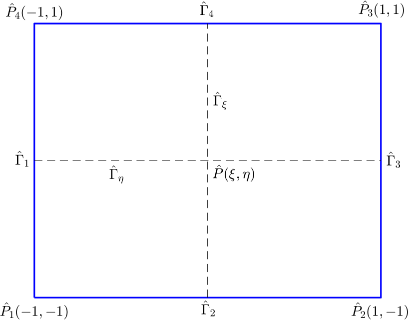
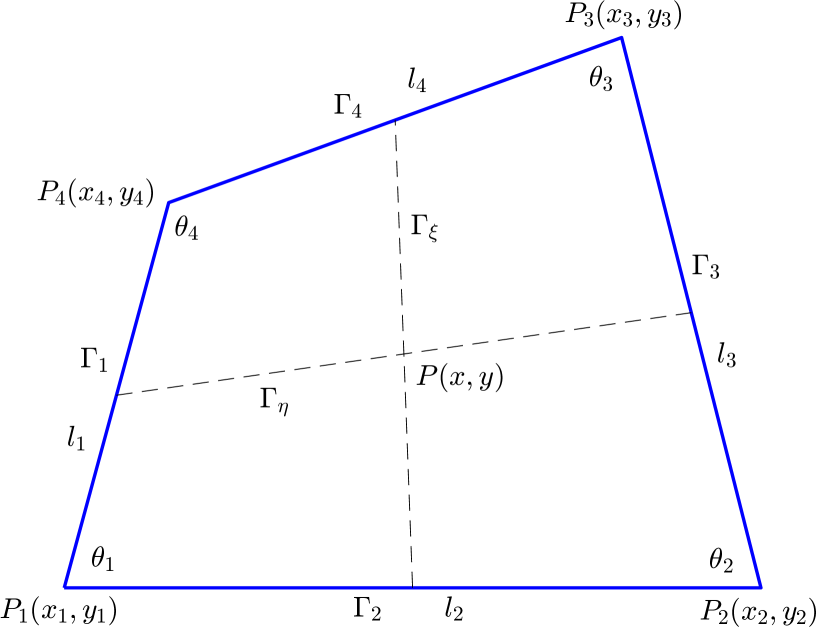
Figure 3.1. Reference square $\hat{K}$(left) and arbitrary convex quadrilateral(right).

(3.1) $$\begin{split}\begin{pmatrix}x\\ y\end{pmatrix}=\Phi_{K}\begin{pmatrix}\hat{x}\\ \hat{y}\end{pmatrix}:&=\sigma_{1}(\hat{x},\hat{y})\begin{pmatrix}x_{1}\\ y_{1}\end{pmatrix}+\sigma_{2}(\hat{x},\hat{y})\begin{pmatrix}x_{2}\\ y_{2}\end{pmatrix}\\ &+\sigma_{3}(\hat{x},\hat{y})\begin{pmatrix}x_{3}\\ y_{3}\end{pmatrix}+\sigma_{4}(\hat{x},\hat{y})\begin{pmatrix}x_{4}\\ y_{4}\end{pmatrix},\qquad(\hat{x},\hat{y})\in\bar{\hat{K}},\,(x,y)\in\bar{K},\end{split}$$

where

$$\sigma_{1}(\hat{x},\hat{y})=\frac{(1-\hat{x})(1-\hat{y})}{4},\ \sigma_{2}(\hat{x},\hat{y})=\frac{(1+\hat{x})(1-\hat{y})}{4},$$

$$\sigma_{3}(\hat{x},\hat{y})=\frac{(1+\hat{x})(1+\hat{y})}{4},\ \sigma_{4}(\hat{x},\hat{y})=\frac{(1-\hat{x})(1+\hat{y})}{4}.$$

For simplicity, we write $x_{ij}=x_{i}-x_{j},\ y_{ij}=y_{i}-y_{j}$ hereafter. Given a scalar function $\phi$ defined on $K$, we associate it with ${\hat{\phi}}:=\phi\circ\Phi_{K}$ on $\hat{K}$. It is easy to see from the chain rule that

(3.2) $$\partial_{\hat{x}}\hat{\phi}=B_{11}(\hat{y})\partial_{x}\phi+B_{21}(\hat{y})\partial_{y}\phi,\quad\partial_{\hat{y}}\hat{\phi}=B_{12}(\hat{x})\partial_{x}\phi+B_{22}(\hat{x})\partial_{y}\phi,$$

where

$$B_{11}=B_{11}(\hat{y}):=\frac{x_{21}}{2}\frac{1-\hat{y}}{2}+\frac{x_{34}}{2}\frac{1+\hat{y}}{2},\quad B_{12}=B_{12}(\hat{x}):=\frac{x_{41}}{2}\frac{1-\hat{x}}{2}+\frac{x_{32}}{2}\frac{1+\hat{x}}{2},$$

$$B_{21}=B_{21}(\hat{y}):=\frac{y_{21}}{2}\frac{1-\hat{y}}{2}+\frac{y_{34}}{2}\frac{1+\hat{y}}{2},\quad B_{22}=B_{22}(\hat{x}):=\frac{y_{41}}{2}\frac{1-\hat{x}}{2}+\frac{y_{32}}{2}\frac{1+\hat{x}}{2}.$$

The Jacobian matrix of the transformation $\Phi_{K}$ with respect to the reference coordinates and its determinant are denoted by

(3.3) $$B_{K}(\hat{x},\hat{y})=\begin{pmatrix}\dfrac{\partial x}{\partial\hat{x}}&\dfrac{\partial x}{\partial\hat{y}}\\[6.99997pt] \dfrac{\partial y}{\partial\hat{x}}&\dfrac{\partial y}{\partial\hat{y}}\end{pmatrix}=\begin{pmatrix}B_{11}&B_{12}\\[6.99997pt] B_{21}&B_{22}\end{pmatrix},\qquad J_{K}(\hat{x},\hat{y})=\det(B_{K}(\hat{x},\hat{y})),\qquad(\hat{x},\hat{y})\in{\hat{K}}.$$

More clearly,

(3.4) $$J_{K}(\hat{x},\hat{y}): =\frac{x_{21}y_{41}-y_{21}x_{41}}{4}\sigma_{1}(\hat{x},\hat{y})+\frac{x_{32}y_{12}-y_{32}x_{12}}{4}\sigma_{2}(\hat{x},\hat{y})$$

$$+\frac{x_{43}y_{23}-y_{43}x_{23}}{4}\sigma_{3}(\hat{x},\hat{y})+\frac{x_{14}y_{34}-y_{14}x_{34}}{4}\sigma_{4}(\hat{x},\hat{y})$$

$$= \,\frac{l_{2}l_{1}\sin\theta_{1}}{4}\sigma_{1}(\hat{x},\hat{y})+\frac{l_{3}l_{2}\sin\theta_{2}}{4}\sigma_{2}(\hat{x},\hat{y})+\frac{l_{4}l_{3}\sin\theta_{3}}{4}\sigma_{3}(\hat{x},\hat{y})+\frac{l_{1}l_{4}\sin\theta_{4}}{4}\sigma_{4}(\hat{x},\hat{y}).$$

Based on the bilinear mapping (3.1), we introduce the contravariant transformation from $H(\text{curl}^{2};\hat{K})$ to $H(\text{curl}^{2};K)$,

(3.5) $$\bm{p}=B_{K}^{-\mathsf{T}}\hat{\bm{p}}\circ\Phi_{K}^{-1},\qquad\hat{\bm{p}}\in H(\text{curl}^{2};\hat{K}).$$

It can be checked from (3.2) that

(3.6) $$\nabla\times\bm{p}=J^{-1}_{K}\hat{\nabla}\times\hat{\bm{p}}\circ\Phi_{K}^{-1},$$

(3.7) $$(\nabla\times)^{2}\bm{p}=\dfrac{B_{K}}{J_{K}^{2}}\left((\hat{\nabla}\times)^{2}\hat{\bm{p}}-\dfrac{\hat{\nabla}\times\hat{\bm{p}}}{J_{K}}\begin{pmatrix}\dfrac{x_{12}+x_{34}}{4}B_{22}-\dfrac{y_{12}+y_{34}}{4}B_{12}\\[6.99997pt] -\dfrac{y_{12}+y_{34}}{4}B_{11}+\dfrac{x_{12}+x_{34}}{4}B_{21}\end{pmatrix}\right)\circ\Phi_{K}^{-1},$$

(3.8) $${\bm{p}}\cdot\bm{\tau}=B_{K}^{-\mathsf{T}}\hat{\bm{p}}\cdot\frac{B_{K}\hat{\bm{\tau}}}{\|B_{K}\hat{\bm{\tau}}\|}\circ\Phi_{K}^{-1}=\frac{\hat{\bm{p}}\cdot\hat{\bm{\tau}}}{\|B_{K}\hat{\bm{\tau}}\|}\circ\Phi_{K}^{-1}.$$

We note that $\|B_{K}\hat{\bm{\tau}}\|=\frac{l_{i}}{2}$ on ${\Gamma_{i}}$ under the bilinear mapping (3.1). Throughout this paper, we always associate a vector field $\bm{\phi}\in H(\text{curl}^{2};K)$ with $\hat{\bm{\phi}}\in H(\text{curl}^{2};\hat{K})$ by the contravariant transformation (3.5).

Remark 3.1.

Note that $\Phi_{K}$ is reduced to affine mapping such that $B_{K}$ is a constant matrix and $J_{K}$ is constant whenever $K$ is a rectangle or a parallelogram. In particular, if $K$ is a rectangle with $\Gamma_{1}$ and $\Gamma_{3}$ (resp. $\Gamma_{2}$ and $\Gamma_{4}$) parallel to the vertical (resp. horizontal) axis, $B_{K}=\mathrm{Diag}\big{(}\frac{l_{2}}{2},\frac{l_{1}}{2}\big{)}$ is a constant diagonal matrix.

3.2. $H(\text{curl}^{2})$-conforming quadrilateral spectral elements

Now we are in a position to present hierarchical basis functions of $H(\text{curl}^{2})$-conforming spectral elements on an unstructured quadrilateral mesh. For simplicity, we shall write $s_{i}:=\sin\theta_{i}$, $i=1,2,3,4$. We emphasize that our desired basis functions, $\bm{\psi}_{m,n},\bm{\phi}_{m,n}$, $m,n\geq 0$, on a quadrilateral element $K$ are obtained from the functions, $\hat{\bm{\psi}}_{m,n},\hat{\bm{\phi}}_{m,n}$, $m,n\geq 0$, in the reference coordinates through the bilinear mapping (3.1) and the contravariant transformation (3.5) such that $\bm{\psi}_{m,n}=B_{K}^{-\mathsf{T}}\hat{\bm{\psi}}_{m,n}\circ\Phi_{K}^{-1}$, and $\bm{\phi}_{m,n}=B_{K}^{-\mathsf{T}}\hat{\bm{\phi}}_{m,n}\circ\Phi_{K}^{-1}$.

Details on the constructions of the $H(\text{curl}^{2})$-conforming quadrilateral elements will be postponed to the next section.

• Interior modes

  (3.9) $$\begin{split}&\hat{\bm{\phi}}_{m,n}=\hat{\nabla}\big{[}K^{-1,-1}_{m}(\hat{x})K^{-1,-1}_{n}(\hat{y})\big{]},\quad m,n\geq 2,\\ &\hat{\bm{\psi}}_{m,n}=\hat{\nabla}K^{-2,-2}_{m}(\hat{x})K^{-2,-2}_{n}(\hat{y}),\quad\ \ m\in\{2,4,5,6,\cdots\},n\geq 4,\\ &\hat{\bm{\psi}}_{m,2}=\hat{K}^{-2,-2}_{m}(\hat{x})\hat{\nabla}\hat{K}^{-2,-2}_{n}(\hat{y}),\quad\ \ m\geq 4,n=2,\end{split}$$

  such that

  $${\bm{\phi}}_{m,n}\cdot{\bm{\tau}}\big{|}_{\Gamma}=[0,0,0,0], \nabla\times{\bm{\phi}}_{m,n}\big{|}_{\Gamma}=[0,0,0,0],$$

  $${\bm{\psi}}_{m,n}\cdot{\bm{\tau}}\big{|}_{\Gamma}=[0,0,0,0], \nabla\times{\bm{\psi}}_{m,n}\big{|}_{\Gamma}=[0,0,0,0].$$

  Hereafter, we use tetrads for the trace on four edges, i.e., $\phi|_{\Gamma}=\left[\phi|_{\Gamma_{1}},\phi|_{\Gamma_{2}},\phi|_{\Gamma_{3}},\phi|_{\Gamma_{4}}\right]$.

• Function edge modes

  • Function edge modes corresponding to $\Gamma_{1}$:

    (3.10) $$\begin{split}&\hat{\bm{\phi}}_{0,n}=\hat{\nabla}\big{[}K^{-1,-1}_{0}(\hat{x})K^{-1,-1}_{n}(\hat{y})\big{]},\quad n\geq 2,\\ &\hat{\bm{\phi}}_{0,0}=\left(\frac{\hat{y}(\hat{y}^{2}-1)\left(3\hat{x}^{2}-5\right)}{32},-\frac{\hat{x}(\hat{x}^{2}-1)\left(3\hat{y}^{2}-5\right)}{32}-\frac{\hat{x}-1}{4}\right)^{\mathsf{T}},\end{split}$$

    such that

    $${\bm{\phi}}_{0,n}\cdot{\bm{\tau}}\big{|}_{\Gamma}=\left[-\frac{(n-1)J^{0,0}_{n-1}(\hat{y})}{l_{1}},0,0,0\right], \nabla\times{\bm{\phi}}_{0,n}\big{|}_{\Gamma}=[0,0,0,0],\quad n\geq 2,$$

    $${\bm{\phi}}_{0,0}\cdot{\bm{\tau}}\big{|}_{\Gamma}=\left[-\frac{1}{l_{1}},0,0,0\right], \nabla\times{\bm{\phi}}_{0,0}\big{|}_{\Gamma}=[0,0,0,0].$$

  • Function edge modes corresponding to $\Gamma_{2}$:

    (3.11) $$\begin{split}&\hat{\bm{\phi}}_{m,0}=\hat{\nabla}\big{[}K^{-1,-1}_{m}(\hat{x})K^{-1,-1}_{0}(\hat{y})\big{]},\quad m\geq 2,\\ &\hat{\bm{\phi}}_{1,0}=\left(-\frac{\hat{y}(\hat{y}^{2}-1)\left(3\hat{x}^{2}-5\right)}{32}-\frac{\hat{y}-1}{4},\frac{\hat{x}(\hat{x}^{2}-1)\left(3\hat{y}^{2}-5\right)}{32}\right)^{\mathsf{T}},\end{split}$$

    such that

    $${\bm{\phi}}_{m,0}\cdot{\bm{\tau}}\big{|}_{\Gamma}=\left[0,\frac{(m-1)J^{0,0}_{m-1}(\hat{x})}{l_{2}},0,0\right], \nabla\times{\bm{\phi}}_{m,0}\big{|}_{\Gamma}=[0,0,0,0],\quad m\geq 2,$$

    $${\bm{\phi}}_{1,0}\cdot{\bm{\tau}}\big{|}_{\Gamma}=\left[0,\frac{1}{l_{2}},0,0\right], \nabla\times{\bm{\phi}}_{1,0}\big{|}_{\Gamma}=[0,0,0,0].$$

  • Function edge modes corresponding to $\Gamma_{3}$:

    (3.12) $$\begin{split}&\hat{\bm{\phi}}_{1,n}=\hat{\nabla}\big{[}K^{-1,-1}_{1}(\hat{x})K^{-1,-1}_{n}(\hat{y})\big{]},\quad n\geq 2,\\ &\hat{\bm{\phi}}_{1,1}=\left(-\frac{\hat{y}(\hat{y}^{2}-1)\left(3\hat{x}^{2}-5\right)}{32},\frac{\hat{x}(\hat{x}^{2}-1)\left(3\hat{y}^{2}-5\right)}{32}+\frac{1+\hat{x}}{4}\right)^{\mathsf{T}},\end{split}$$

    such that

    $${\bm{\phi}}_{1,n}\cdot{\bm{\tau}}\big{|}_{\Gamma}=\left[0,0,\frac{(n-1)J^{0,0}_{n-1}(\hat{y})}{l_{3}},0\right], \nabla\times{\bm{\phi}}_{1,n}\big{|}_{\Gamma}=[0,0,0,0],\quad n\geq 2,$$

    $${\bm{\phi}}_{1,1}\cdot{\bm{\tau}}\big{|}_{\Gamma}=\left[0,0,\frac{1}{l_{3}},0\right], \nabla\times{\bm{\phi}}_{1,1}\big{|}_{\Gamma}=[0,0,0,0].$$

  • Function edge modes corresponding to $\Gamma_{4}$:

    (3.13) $$\begin{split}&\hat{\bm{\phi}}_{m,1}=\hat{\nabla}\big{[}K^{-1,-1}_{m}(\hat{x})K^{-1,-1}_{1}(\hat{y})\big{]},\quad m\geq 2,\\ &\hat{\bm{\phi}}_{0,1}=\left(\frac{\hat{y}(\hat{y}^{2}-1)\left(3\hat{x}^{2}-5\right)}{32}+\frac{1+\hat{y}}{4},-\frac{\hat{x}(\hat{x}^{2}-1)\left(3\hat{y}^{2}-5\right)}{32}\right)^{\mathsf{T}},\end{split}$$

    such that

    $${\bm{\phi}}_{m,1}\cdot{\bm{\tau}}\big{|}_{\Gamma}=\left[0,0,0,-\frac{(m-1)J^{0,0}_{m-1}(\hat{x})}{l_{4}}\right], \nabla\times{\bm{\phi}}_{m,1}\big{|}_{\Gamma}=[0,0,0,0],\quad m\geq 2,$$

    $${\bm{\phi}}_{0,1}\cdot{\bm{\tau}}\big{|}_{\Gamma}=\left[0,0,0,-\frac{1}{l_{4}}\right], \nabla\times{\bm{\phi}}_{0,1}\big{|}_{\Gamma}=[0,0,0,0].$$

  By adding a multiple of the interior mode $\hat{\bm{\phi}}_{3,3}$ to each basis functions, one obtains four alternative function edge modes $\hat{\tilde{\bm{\phi}}}_{0,0},\,\hat{\tilde{\bm{\phi}}}_{1,0},\,\hat{\tilde{\bm{\phi}}}_{1,1}$ and $\hat{\tilde{\bm{\phi}}}_{0,1}$ with even simple presentations:

  $$\hat{\tilde{\bm{\phi}}}_{0,0}=\hat{\bm{\phi}}_{0,0}+\frac{\hat{\bm{\phi}}_{3,3}}{8}=\left(\frac{3\hat{y}(\hat{y}^{2}-1)(\hat{x}^{2}-1)}{16},\frac{(\hat{x}+2)(\hat{x}-1)^{2}}{8}\right)^{\mathsf{T}},$$

  $$\hat{\tilde{\bm{\phi}}}_{1,0}=\hat{\bm{\phi}}_{1,0}+\frac{\hat{\bm{\phi}}_{3,3}}{8}=\left(\frac{(\hat{y}+2)(\hat{y}-1)^{2}}{8},\frac{3x(x^{2}-1)(\hat{y}^{2}-1)}{16}\right)^{\mathsf{T}},$$

  $$\hat{\tilde{\bm{\phi}}}_{1,1}=\hat{\bm{\phi}}_{1,1}-\frac{\hat{\bm{\phi}}_{3,3}}{8}=\left(-\frac{3\hat{y}(\hat{y}^{2}-1)(\hat{x}^{2}-1)}{16},-\frac{(\hat{x}-2)(\hat{x}+1)^{2}}{8}\right)^{\mathsf{T}},$$

  $$\hat{\tilde{\bm{\phi}}}_{0,1}=\hat{\bm{\phi}}_{0,1}-\frac{\hat{\bm{\phi}}_{3,3}}{8}=\left(-\frac{(\hat{y}-2)(\hat{y}+1)^{2}}{8},-\frac{3\hat{x}(\hat{x}^{2}-1)(\hat{y}^{2}-1)}{16}\right)^{\mathsf{T}}.$$

• Curl boundary modes

  • Curl edge modes corresponding to $\Gamma_{1}$:

    (3.14) $$\bm{\hat{\psi}}_{1,n}=J_{K}(\hat{x},\hat{y})K^{-2,-2}_{1}(\hat{x})\hat{\nabla}K^{-2,-2}_{n}(\hat{y}),\quad n\in\{2,4,5,6,\cdots\},$$

    such that

    $${\bm{\psi}}_{1,n}\cdot{\bm{\tau}}\big{|}_{\Gamma}=[0,0,0,0], \nabla\times{\bm{\psi}}_{1,n}\big{|}_{\Gamma}=[K^{-2,-2}_{n}{}^{\prime}(\hat{y}),0,0,0].$$

  • Curl edge modes corresponding to $\Gamma_{2}$:

    (3.15) $$\bm{\hat{\psi}}_{m,1}=J_{K}(\hat{x},\hat{y})\hat{\nabla}K^{-2,-2}_{m}(\hat{x})K^{-2,-2}_{1}(\hat{y}),\quad m\in\{2,4,5,6,\cdots\},$$

    such that

    $${\bm{\psi}}_{m,1}\cdot{\bm{\tau}}\big{|}_{\Gamma}=[0,0,0,0], \nabla\times{\bm{\psi}}_{m,1}\big{|}_{\Gamma}=[0,-K^{-2,-2}_{m}{}^{\prime}(\hat{x}),0,0].$$

  • Curl edge modes corresponding to $\Gamma_{3}$:

    (3.16) $$\bm{\hat{\psi}}_{3,n}=J_{K}(\hat{x},\hat{y})K^{-2,-2}_{3}(\hat{x})\hat{\nabla}K^{-2,-2}_{n}(\hat{y}),\quad n\in\{2,4,5,6,\cdots\},$$

    such that

    $${\bm{\psi}}_{3,n}\cdot{\bm{\tau}}\big{|}_{\Gamma}=[0,0,0,0], \nabla\times{\bm{\psi}}_{3,n}\big{|}_{\Gamma}=[0,0,K^{-2,-2}_{n}{}^{\prime}(\hat{y}),0].$$

  • Curl edge modes corresponding to $\Gamma_{4}$:

    (3.17) $$\bm{\hat{\psi}}_{m,3}=J_{K}(\hat{x},\hat{y})\hat{\nabla}K^{-2,-2}_{m}(\hat{x})K^{-2,-2}_{3}(\hat{y}),\quad m\in\{2,4,5,6,\cdots\},$$

    such that

    $${\bm{\psi}}_{m,3}\cdot{\bm{\tau}}\big{|}_{\Gamma}=[0,0,0,0], \nabla\times{\bm{\psi}}_{m,3}\big{|}_{\Gamma}=[0,0,0,-K^{-2,-2}_{m}{}^{\prime}(\hat{x})].$$

  Whenever $K$ is a rectangle or a parallelogram, $J_{K}(\hat{x},\hat{y})=\frac{|K|}{4}$, where $|K|$ stands for the area of $K$.

• Vertex modes

  • Vertex modes corresponding to $P_{1}$:

    (3.18) $$\begin{split}\bm{\hat{\psi}}_{0,0}=\Bigg{(}&(\hat{y}-1)^{2}(1+\hat{y})(\hat{x}-1)\left(\frac{l_{2}\left(l_{1}s_{1}+2l_{3}s_{2}\right)\hat{x}}{128}+\frac{l_{2}\left(3l_{1}s_{1}+2l_{3}s_{2}\right)}{128}\right),\\ &-(1+\hat{x})(\hat{y}-1)(\hat{x}-1)^{2}\left(\frac{l_{1}\left(l_{2}s_{1}+2l_{4}s_{4}\right)\hat{y}}{128}+\frac{l_{1}\left(3l_{2}s_{1}+2l_{4}s_{4}\right)}{128}\right)\Bigg{)}^{\mathsf{T}},\end{split}$$

    such that

    $${\bm{\psi}}_{0,0}\cdot{\bm{\tau}}\big{|}_{\Gamma}=[0,0,0,0], \nabla\times{\bm{\psi}}_{0,0}\big{|}_{\Gamma}=\left[-\frac{\hat{y}}{2}+\frac{1}{2},\frac{1}{2}-\frac{\hat{x}}{2},0,0\right].$$

  • Vertex modes corresponding to $P_{2}$:

    (3.19) $$\begin{split}\bm{\hat{\psi}}_{0,1}=\Bigg{(}&(\hat{y}-1)^{2}(1+\hat{y})(\hat{x}+1)\left(\frac{l_{2}\left(2l_{1}s_{1}+l_{3}s_{2}\right)\hat{x}}{128}-\frac{l_{2}\left(2l_{1}s_{1}+3l_{3}s_{2}\right)}{128}\right),\\ &(1-\hat{x})(\hat{y}-1)(1+\hat{x})^{2}\left(\frac{l_{3}\left(l_{2}s_{2}+2l_{4}s_{3}\right)\hat{y}}{128}+\frac{l_{3}\left(3l_{2}s_{2}+2l_{4}s_{3}\right)}{128}\right)\Bigg{)}^{\mathsf{T}},\end{split}$$

    such that

    $${\bm{\psi}}_{0,1}\cdot{\bm{\tau}}\big{|}_{\Gamma}=[0,0,0,0], \nabla\times{\bm{\psi}}_{0,1}\big{|}_{\Gamma}=\left[0,\frac{1}{2}+\frac{\hat{x}}{2},-\frac{\hat{y}}{2}+\frac{1}{2},0\right].$$

  • Vertex modes corresponding to $P_{3}$:

    (3.20) $$\begin{split}\bm{\hat{\psi}}_{1,1}=\Bigg{(}&(\hat{y}+1)^{2}(1-\hat{y})(\hat{x}+1)\left(-\frac{l_{4}\left(2l_{1}s_{4}+l_{3}s_{3}\right)\hat{x}}{128}+\frac{l_{4}\left(2l_{1}s_{4}+3l_{3}s_{3}\right)}{128}\right),\\ &(1-\hat{x})(\hat{y}+1)(\hat{x}+1)^{2}\left(\frac{l_{3}\left(2l_{2}s_{2}+l_{4}s_{3}\right)\hat{y}}{128}-\frac{l_{3}\left(2l_{2}s_{2}+3l_{4}s_{3}\right)}{128}\right)\Bigg{)}^{\mathsf{T}},\end{split}$$

    such that

    $${\bm{\psi}}_{1,1}\cdot{\bm{\tau}}\big{|}_{\Gamma}=[0,0,0,0], \nabla\times{\bm{\psi}}_{1,1}\big{|}_{\Gamma}=\left[0,0,\frac{1}{2}+\frac{\hat{y}}{2},\frac{1}{2}+\frac{\hat{x}}{2}\right].$$

  • Vertex modes corresponding to $P_{4}$:

    (3.21) $$\begin{split}\bm{\hat{\psi}}_{1,0}=&\Bigg{(}(\hat{y}+1)^{2}(1-\hat{y})(\hat{x}-1)\left(-\frac{l_{4}\left(l_{1}s_{4}+2l_{3}s_{3}\right)\hat{x}}{128}-\frac{l_{4}\left(3l_{1}s_{4}+2l_{3}s_{3}\right)}{128}\right),\\ &(1+\hat{x})(\hat{y}+1)(\hat{x}-1)^{2}\left(-\frac{l_{1}\left(2l_{2}s_{1}+l_{4}s_{4}\right)\hat{y}}{128}+\frac{l_{1}\left(2l_{2}s_{1}+3l_{4}s_{4}\right)}{128}\right)\Bigg{)}^{\mathsf{T}},\end{split}$$

    such that

    $${\bm{\psi}}_{1,0}\cdot{\bm{\tau}}\big{|}_{\Gamma}=[0,0,0,0], \nabla\times{\bm{\psi}}_{1,0}\big{|}_{\Gamma}=\left[\frac{1}{2}+\frac{\hat{y}}{2},0,0,\frac{1}{2}-\frac{\hat{x}}{2}\right].$$

  Whenever $K$ is a rectangle or parallelogram, $\bm{\hat{\psi}}_{0,0},\bm{\hat{\psi}}_{0,1},\bm{\hat{\psi}}_{1,1},\bm{\hat{\psi}}_{1,0}$ are reduced to

  $$\bm{\hat{\psi}}_{0,0}=\left(\frac{|K|(\hat{y}-1)^{2}(\hat{y}+1)(\hat{x}-1)\left(3\hat{x}+5\right)}{128},-\frac{|K|(\hat{x}+1)(\hat{y}-1)(\hat{x}-1)^{2}\left(3\hat{y}+5\right)}{128}\right)^{\mathsf{T}},$$

  $$\bm{\hat{\psi}}_{0,1}=\left(\frac{|K|(\hat{y}-1)^{2}(\hat{y}+1)(\hat{x}+1)\left(3\hat{x}-5\right)}{128},-\frac{|K|(\hat{x}-1)(\hat{y}-1)(\hat{x}+1)^{2}\left(3\hat{y}+5\right)}{128}\right)^{\mathsf{T}},$$

  $$\bm{\hat{\psi}}_{1,1}=\Bigg{(}\frac{|K|(\hat{y}+1)^{2}(\hat{y}-1)(\hat{x}+1)\left(3\hat{x}-5\right)}{128},-\frac{|K|(\hat{x}-1)(\hat{y}+1)(\hat{x}+1)^{2}\left(3\hat{y}-5\right)}{128}\Bigg{)}^{\mathsf{T}},$$

  $$\bm{\hat{\psi}}_{1,0}=\Bigg{(}\frac{|K|(\hat{y}+1)^{2}(\hat{y}-1)(\hat{x}-1)\left(3\hat{x}+5\right)}{128},-\frac{|K|(\hat{x}+1)(\hat{y}+1)(\hat{x}-1)^{2}\left(3\hat{y}-5\right)}{128}\Bigg{)}^{\mathsf{T}},$$

  respectively.

4. Constructions of the $H(\text{curl}^{2})$-conforming quadrilateral spectral elements

In this section, we show the derivation process of $H(\text{curl}^{2})$-conforming basis functions on a quadrilateral element $K$ from basis functions for vector fields on the reference square $\hat{K}$ through the bilinear mapping (3.1) and the contravariant transformation (3.5).

We first resort to the following de Rham complex [1, 11] for an enlightenment of the construction process,

(4.1) $$\mathbb{R} \overset{id}{\longrightarrow} H^{1}(\Omega) \overset{\nabla}{\longrightarrow} H(\text{curl}^{2};\Omega) \overset{\nabla\times}{\longrightarrow} \quad H^{1}(\Omega) \overset{0}{\longrightarrow} \{0\}$$

$$\quad\cup \quad\quad\cup \quad\quad\cup$$

$$\mathbb{R} \overset{id}{\longrightarrow} \quad S_{h} \overset{\nabla}{\longrightarrow} \quad\quad W_{h} \overset{\nabla\times}{\longrightarrow} \quad\quad U_{h} \overset{0}{\longrightarrow} \{0\},$$

where $S_{h}=\left\{u_{h}\in H^{1}(\Omega):u_{h}\big{|}_{K}\circ\Phi^{-1}_{K}\text{ is certain bivariate polynomial for all }K\in\mathcal{T}_{h}\right\}$, and $W_{h},U_{h}$ are certain conforming element spaces over the partition $\mathcal{T}_{h}$ of $\Omega$. The main property of the de Rham complex lies in that the range of each operator coincides with the kernel of the following operator consecutive operators. In particular,

(4.2) $$\begin{aligned} &H(\text{curl}^{2};\Omega)&&\supseteq\left\{\bm{u}\in H(\text{curl}^{2};\Omega):\nabla\times\bm{u}=0\right\}&&=\nabla H^{1}(\Omega)&&\supseteq\nabla H^{2}(\Omega),\\ &W_{h}&&\supseteq\left\{\bm{u}\in W_{h}:\nabla\times\bm{u}=0\right\}&&=\nabla S_{h}&&\supseteq\nabla\left[S_{h}\cap H^{2}(\Omega)\right].\end{aligned}$$

4.1. Vectorial basis functions on the reference square

It is known that $K^{-1,-1}_{m}(\hat{x})K^{-1,-1}_{n}(\hat{y})$, $m,n\geq 0$ are basis functions on the reference square $\hat{K}$ for constructing $C^{1}$-conforming spectral elements using the bilinear mapping (3.1) over quadrilateral partitions [12]. According to (4.2) and (3.2), $\bm{B}_{K}^{-\mathsf{T}}\hat{\nabla}\left[K^{-1,-1}_{m}(\hat{x})K^{-1,-1}_{n}(\hat{y})\right]\circ\Phi_{K}^{-1},\ m,n\geq 0,$ are local basis candidates on $K$ for the discrete kernel space $\left\{\bm{u}\in V_{h}:\nabla\times\bm{u}=0\right\}$. For this reason, we would like to choose

(4.3) $$\hat{\bm{p}}_{m,n}(\hat{x},\hat{y}):=\hat{\nabla}\big{[}K^{-1,-1}_{m}(\hat{x})K^{-1,-1}_{n}(\hat{y})\big{]},\quad(m,n)\in\mathbb{N}_{0}^{2}\setminus\{(0,0)\},$$

as a part of vectorial basis functions on the reference square.

Inspired by the success of the work in [28], we recommend

(4.4) $$\hat{\bm{q}}_{m,n}(\hat{x},\hat{y}):=\hat{\nabla}K^{-2,-2}_{m}(\hat{x})K^{-2,-2}_{n}(\hat{y})\ \text{ or }\ \hat{\bm{q}}_{m,n}^{\ast}(\hat{x},\hat{y}):=K^{-2,-2}_{m}(\hat{x})\hat{\nabla}K^{-2,-2}_{n}(\hat{y}),\quad(m,n)\in\mathbb{N}^{2},$$

for the other part of vectorial basis functions on the reference square.

It is easy to see that $\hat{\bm{q}}_{0,n}+\hat{\bm{q}}_{2,n}=\hat{\bm{q}}^{\ast}_{m,0}+\hat{\bm{q}}^{\ast}_{m,2}=0$ for any $m,n\in\mathbb{N}_{0}$, and

$$\hat{\bm{q}}_{m,n}+\hat{\bm{q}}_{m,n}^{\ast}=\hat{\nabla}[\hat{K}^{-2,-2}_{m}(\hat{x})K^{-2,-2}_{n}(\hat{y})],$$

$$\hat{\bm{q}}_{m,0}+\hat{\bm{q}}_{m,2}=\hat{\nabla}[\hat{K}^{-2,-2}_{m}(\hat{x})], \hat{\bm{q}}^{\ast}_{0,n}+\hat{\bm{q}}^{\ast}_{2,n}=\hat{\nabla}[\hat{K}^{-2,-2}_{n}(\hat{y})],$$

are all finite linear combination of $\hat{\bm{p}}_{i,j}$, $(i,j)\in\mathbb{N}_{0}^{2}\setminus\{(0,0)\}$ for any $m,n\in\mathbb{N}_{0}$. Thus two parts of vectorial functions $\hat{\bm{p}}_{m,n}$, $(m,n)\in\mathbb{N}_{0}^{2}\setminus\{(0,0)\}$, and $\hat{\bm{q}}_{m,n}/\hat{\bm{q}}^{\ast}_{m,n}$, $(m,n)\in\mathbb{N}^{2}$, form a basis in $[L^{2}(\hat{K})]^{2}$.

Now we are ready to present the trace properties of the vectorial basis functions under the contravariant transformation (3.5). The following three lemmas can be deduced from the definition of the general Jacobi polynomials (2.1), and their properties (2.2)-(2.6) immediately.

Lemma 4.1.

Let $\bm{p}_{{m,n}}=B_{K}^{-\mathsf{T}}\hat{\bm{p}}_{{m,n}}\circ\Phi_{K}^{-1}$, and it holds that

(4.5) $$\nabla\times\bm{p}_{{m,n}}= \,0,$$

(4.6) $$\begin{split}\bm{p}_{{m,n}}\cdot\bm{\tau}\big{|}_{\Gamma}=&\Bigg{[}-\frac{2K^{-1,-1}_{m}(-1)K^{-1,-1}_{n}{}^{\prime}(\hat{y})}{l_{1}},\frac{2K^{-1,-1}_{m}{}^{\prime}(\hat{x})K^{-1,-1}_{n}(-1)}{l_{2}},\\ &\quad\frac{2K^{-1,-1}_{m}(1)K^{-1,-1}_{n}{}^{\prime}(\hat{y})}{l_{3}},-\frac{2K^{-1,-1}_{m}{}^{\prime}(\hat{x})K^{-1,-1}_{n}(1)}{l_{4}}\Bigg{]}\\ =&\begin{cases}[0,0,0,0],&m\geq 2,\,n\geq 2,\\ [-\frac{(n-1)J^{0,0}_{n-1}(\hat{y})}{l_{1}},0,0,0],&m=0,\,n\geq 2,\\ [0,0,\frac{(n-1)J^{0,0}_{n-1}(\hat{y})}{l_{3}},0],&m=1,\,n\geq 2,\\ [0,\frac{(m-1)J^{0,0}_{m-1}(\hat{x})}{l_{2}},0,0],&m\geq 2,\,n=0,\\ [0,0,0,-\frac{(m-1)J^{0,0}_{m-1}(\hat{x})}{l_{4}}],&m\geq 2,\,n=1,\\ [\frac{1}{l_{1}},-\frac{1}{l_{2}},0,0],&m=0,\,n=0,\\ [0,\frac{1}{l_{2}},-\frac{1}{l_{3}},0],&m=1,\,n=0,\\ [0,0,\frac{1}{l_{3}},-\frac{1}{l_{4}}],&m=1,\,n=1,\\ [-\frac{1}{l_{1}},0,0,\frac{1}{l_{4}}],&m=0,\,n=1.\end{cases}\end{split}$$

Lemma 4.2.

Let ${\bm{q}}_{{m,n}}=B_{K}^{-\mathsf{T}}\hat{\bm{q}}_{{m,n}}\circ\Phi_{K}^{-1}$, then it holds that

(4.7) $$\begin{split}{\bm{q}}_{{m,n}}\cdot\bm{\tau}\big{|}_{\Gamma}=&\,\left[0,\frac{2K^{-2,-2}_{m}{}^{\prime}(\hat{x})K^{-2,-2}_{n}(-1)}{l_{2}},0,-\frac{2K^{-2,-2}_{m}{}^{\prime}(\hat{x})K^{-2,-2}_{n}(1)}{l_{4}}\right]\\ =&\begin{cases}[0,0,0,0],&m\geq 1,\,n\in\{1,3,4,5,6,\cdots\},\\ \left[0,0,0,-\frac{2K^{-2,-2}_{m}{}^{\prime}(\hat{x})}{l_{4}}\right],&m\geq 1,\,n=2,\end{cases}\end{split}$$

(4.8) $$\begin{split}\nabla\times{\bm{q}}_{{m,n}}|_{\Gamma}=&\,-J^{-1}_{K}(\hat{x},\hat{y})K^{-2,-2}_{m}{}^{\prime}(\hat{x})K^{-2,-2}_{n}{}^{\prime}(\hat{y})\big{|}_{\Gamma}\\ =&\begin{cases}[0,0,0,0],&m,n\in\{2,4,5,6,\cdots\},\\ \left[-\frac{K^{-2,-2}_{n}{}^{\prime}(\hat{y})}{J_{K}(-1,\hat{y})},0,0,0\right],&m=1,\ n\in\{2,4,5,6,\cdots\},\\ \left[0,0,-\frac{K^{-2,-2}_{n}{}^{\prime}(\hat{y})}{J_{K}(1,\hat{y})},0\right],&m=3,\ n\in\{2,4,5,6,\cdots\},\\ \left[0,-\frac{K^{-2,-2}_{m}{}^{\prime}(\hat{x})}{J_{K}(\hat{x},-1)},0,0\right],&n=1,\ m\in\{2,4,5,6,\cdots\},\\ \left[0,0,0,-\frac{K^{-2,-2}_{m}{}^{\prime}(\hat{x})}{J_{K}(\hat{x},1)}\right],&n=3,\ m\in\{2,4,5,6,\cdots\},\\ \left[-\frac{K^{-2,-2}_{1}{}^{\prime}(\hat{y})}{J_{K}(-1,\hat{y})},-\frac{K^{-2,-2}_{1}{}^{\prime}(\hat{x})}{J_{K}(\hat{x},-1)},0,0\right],&m=1,\ n=1,\\ \left[0,-\frac{K^{-2,-2}_{3}{}^{\prime}(\hat{x})}{J_{K}(\hat{x},-1)},-\frac{K^{-2,-2}_{1}{}^{\prime}(\hat{y})}{J_{K}(1,\hat{y})},0\right],&m=3,\ n=1,\\ \left[0,0,-\frac{K^{-2,-2}_{3}{}^{\prime}(\hat{y})}{J_{K}(1,\hat{y})},-\frac{K^{-2,-2}_{3}{}^{\prime}(\hat{x})}{J_{K}(\hat{x},1)}\right],&m=3,\ n=3,\\ \left[-\frac{K^{-2,-2}_{3}{}^{\prime}(\hat{y})}{J_{K}(-1,\hat{y})},0,0,-\frac{K^{-2,-2}_{1}{}^{\prime}(\hat{x})}{J_{K}(\hat{x},1)}\right],&m=1,\ n=3.\end{cases}\end{split}$$

Lemma 4.3.

Let  ${\bm{q}}_{{m,n}}^{\ast}=B_{K}^{-\mathsf{T}}\hat{\bm{q}}_{{m,n}}^{\ast}\circ\Phi_{K}^{-1}$, then we have

(4.9) $$\begin{split}{\bm{q}_{{m,n}}^{\ast}}\cdot\bm{\tau}\big{|}_{\Gamma}=&\,\left[-\frac{2K^{-2,-2}_{m}{}(-1)K^{-2,-2}_{n}{}^{\prime}(\hat{y})}{l_{1}},0,\frac{2K^{-2,-2}_{m}(1)K^{-2,-2}_{n}{}^{\prime}(\hat{y})}{l_{3}},0\right]\\ =&\begin{cases}[0,0,0,0],&n\geq 1,\,m\in\{1,3,4,5,6,\cdots\},\\ [0,0,\frac{2K^{-2,-2}_{n}{}^{\prime}(\hat{y})}{l_{3}},0],&n\geq 1,\,m=2,\end{cases}\end{split}$$

(4.10) $$\nabla\times\bm{q}_{{m,n}}^{\ast}\big{|}_{\Gamma}= \,J^{-1}_{K}(\hat{x},\hat{y})K^{-2,-2}_{m}{}^{\prime}(\hat{x})K^{-2,-2}_{n}{}^{\prime}(\hat{y})\big{|}_{\Gamma}=-\nabla\times\bm{q}_{{m,n}}\big{|}_{\Gamma}.$$

Based on Lemma 4.1 - Lemma 4.3, we shall show in the subsequent subsections how to construct our $H(\operatorname{curl}^{2})$-conforming quadrilateral spectral elements through basis functions (4.3) and (4.4) on the reference square.

4.2. Construction of interior modes

The interior modes are readily constructed by looking up the trace properties of $\hat{\bm{p}}_{m,n}$, $\hat{\bm{q}}_{m,n}$ and $\hat{\bm{q}}^{*}_{m,n}$ in Lemmas 4.1-4.3.

Indeed, (4.5) and (4.6) state that both $\nabla\times\bm{p}_{{m,n}}\big{|}_{\Gamma}$ and $\bm{p}_{{m,n}}\cdot\bm{\tau}\big{|}_{\Gamma}$ vanish if and only if $m,n\geq 2$. While (4.7) and (4.8) (resp. (4.9) and (4.10)) imply that $\bm{q}_{{m,n}}\cdot\bm{\tau}\big{|}_{\Gamma}$ and $\nabla\times\bm{q}_{{m,n}}\big{|}_{\Gamma}$ (resp. $\bm{q}^{\ast}_{{m,n}}\cdot\bm{\tau}\big{|}_{\Gamma}$ and $\nabla\times\bm{q}^{\ast}_{{m,n}}\big{|}_{\Gamma}$) vanish if and only if $m\in\{2,4,5,6,\cdots\},n\geq 4$ (resp. $n\in\{2,4,5,6,\cdots\},m\geq 4$).

By removing the redundant ones, we obtain the interior modes on $K$,

$${\bm{\phi}}_{m,n}(x,y):={\bm{p}}_{m,n}(x,y)=\bm{B}_{K}^{-\mathsf{T}}\hat{\nabla}[K^{-1,-1}_{m}(\hat{x})K^{-1,-1}_{n}(\hat{y})]\circ\Phi_{K}^{-1},\quad m,n\geq 2,$$

$${\bm{\psi}}_{m,n}(x,y):={\bm{q}}_{m,n}(x,y)=\bm{B}_{K}^{-\mathsf{T}}[\hat{\nabla}K^{-2,-2}_{m}(\hat{x})K^{-2,-2}_{n}(\hat{y})]\circ\Phi_{K}^{-1},\quad m\in\{2,4,5,6,\cdots\},n\geq 4,$$

$${\bm{\psi}}_{m,2}(x,y):={\bm{q}}^{\ast}_{m,n}(x,y)=\bm{B}_{K}^{-\mathsf{T}}[\hat{K}^{-2,-2}_{m}(\hat{x})\hat{\nabla}\hat{K}^{-2,-2}_{n}(\hat{y})]\circ\Phi_{K}^{-1},\quad m\geq 4,n=2.$$

4.3. Construction of edge modes

The edge modes should be divided into two types: function edge modes and curl edge modes. We start with the function edge modes. Thanks to Lemma 4.1, the functions

$${\bm{\phi}}_{0,n}=\bm{B}_{K}^{-\mathsf{T}}\hat{\nabla}\big{[}K^{-1,-1}_{0}(\hat{x})K^{-1,-1}_{n}(\hat{y})\big{]}\circ\Phi_{K}^{-1},\ n\geq 2,$$

satisfy the criteria for function edge modes corresponding to $\Gamma_{1}$.

Furthermore, according to Lemma 4.1, Lemma 4.2, and (2.6), we define

$$\hat{\tilde{\bm{\phi}}}_{0,0}=\hat{\nabla}\big{[}K^{-1,-1}_{0}(\hat{x})K^{-1,-1}_{1}(\hat{y})\big{]}+\frac{1}{2}\hat{\nabla}\big{[}K^{-1,-1}_{3}(\hat{x})K^{-1,-1}_{1}(\hat{y})\big{]}+\hat{\nabla}K^{-2,-2}_{2}(\hat{x})K^{-2,-2}_{2}(\hat{y})$$

$$\qquad=\left(\frac{3y(y^{2}-1)(x^{2}-1)}{16},\frac{(x+2)(x-1)^{2}}{8}\right)^{\mathsf{T}},$$

and then find that

$${\tilde{\bm{\phi}}}_{0,0}\cdot\bm{\tau}|_{\Gamma}=\left[-\frac{1}{l_{1}},0,0,0\right], \nabla\times{\tilde{\bm{\phi}}}_{0,0}|_{\Gamma}=\left[0,0,0,0\right].$$

Hence, ${\tilde{\bm{\phi}}}_{0,0}=\bm{B}_{K}^{-\mathsf{T}}\hat{\tilde{\bm{\phi}}}_{0,0}\circ\Phi_{K}^{-1}$ or ${\bm{\phi}}_{0,0}=\bm{B}_{K}^{-\mathsf{T}}\hat{\bm{\phi}}_{0,0}\circ\Phi_{K}^{-1}:=\bm{B}_{K}^{-\mathsf{T}}\big{(}\hat{\tilde{\bm{\phi}}}_{0,0}-\frac{1}{8}\hat{\bm{\phi}}_{3,3}\big{)}\circ\Phi_{K}^{-1}={\tilde{\bm{\phi}}}_{0,0}-{\bm{\phi}}_{3,3}$ is another function edge basis function for $\Gamma_{1}$.

The function edge modes corresponding to $\Gamma_{2},\Gamma_{3}$ and $\Gamma_{4}$ can be obtained by making use of the geometrical and algebraic symmetry.

Next, let us concentrate on the construction of curl edge modes. By Lemma 4.3, we find that $\bm{q}^{\ast}_{1,n}=\bm{B}_{K}^{-\mathsf{T}}[K^{-2,-2}_{1}(\hat{x})\hat{\nabla}K^{-2,-2}_{n}(\hat{y})]\circ\Phi_{K}^{-1},\ n\in\{2,4,5,6,\cdots\},$ satisfy

$$\bm{q}^{\ast}_{1,n}\cdot\bm{\tau}|_{\Gamma}=[0,0,0,0], \nabla\times\bm{q}^{\ast}_{1,n}|_{\Gamma}=\left[\frac{1}{J_{K}(-1,\hat{y})}K_{n}^{-2,-2}{}^{\prime}(\hat{y}),0,0,0\right].$$

Since

$$J_{K}|_{\Gamma_{1}}=\frac{1}{8}\left[l_{2}l_{1}\sin\theta_{1}(1-\hat{y})+l_{1}l_{4}\sin\theta_{4}(1+\hat{y})\right],$$

we observe that the curl trace of $\bm{q}^{\ast}_{1,n}$ on $\Gamma_{1}$ relies on the geometric quantities $l_{1},l_{2},l_{4},\theta_{1},$ and $\theta_{4}$. While the traces, up to first order, of a typical $H(\text{curl}^{2})$-conforming basis functions on $\Gamma_{i}$ only rely on geometric quantities of the edge $\Gamma_{i}$. This motivates us to add a multiplier $J_{K}(\hat{x},\hat{y})$ to the above basis functions, and define

$$\bm{\hat{\psi}}_{1,n}=J_{K}(\hat{x},\hat{y})K^{-2,-2}_{1}(\hat{x})\hat{\nabla}K^{-2,-2}_{n}(\hat{y}),\quad n\in\{2,4,5,6,\cdots\}.$$

which finally lead to all curl edge modes $\bm{\psi}_{1,n}=\bm{B}_{K}^{-\mathsf{T}}\bm{\hat{\psi}}_{1,n}\circ\Phi_{K}^{-1},\ n\in\{2,4,5,6,\cdots\}$, corresponding to $\Gamma_{1}$ on $K$ such that

$$\bm{\psi}_{1,n}\cdot\bm{\tau}|_{\Gamma}=[0,0,0,0], \nabla\times\bm{\psi}_{1,n}|_{\Gamma}=[K_{n}^{-2,-2}{}^{\prime}(\hat{y}),0,0,0],\quad n\ \in\{2,4,5,6,\cdots\}.$$

Similarly, we can obtain other curl edge modes directly by Lemma 4.2-Lemma 4.3.

4.4. Construction of vertex modes

In view of (3.10)-(3.13), the tangent traces of all function edge modes on $K$ form a complete system in $L^{2}(\partial K)$. To make the curl traces of all $H(\operatorname{curl}^{2})$-conforming basis functions on $K$ a complete system in $C^{1}(\partial K)$ in regard to (3.14)-(3.17), we still need four vertex modes whose tangent traces and curl traces along $\Gamma$ are zero and piecewise linear hat functions along $\partial K$, respectivley.

Suppose ${\bm{\psi}}_{0,0}=\bm{B}_{K}^{-\mathsf{T}}\hat{\bm{\psi}}_{0,0}\circ\Phi_{K}^{-1}$ with

(4.11) $$\hat{\bm{\psi}}_{0,0}=\sum_{1\leq m\leq 3}\sum_{n\in\{1,3\}}\left(a_{m,n}\hat{\bm{q}}_{m,n}+b_{m,n}\hat{\bm{q}}^{\ast}_{n,m}\right),$$

is such a basis function at the vertex $P_{1}$. It is then expected that

$${\bm{\psi}}_{0,0}\cdot\bm{\tau}|_{\Gamma}=[0,0,0,0],\qquad\nabla\times\bm{\psi}_{0,0}=\left[\frac{1-\hat{y}}{2},\frac{1-\hat{x}}{2},0,0\right].$$

Indeed, above requirements can be fulfilled if $a_{m,n}$ and $b_{m,n}$ satisfy the following equation,

(4.12) $$\begin{split}\Big{[}\frac{1-\hat{y}}{2},&\frac{1-\hat{x}}{2},0,0\Big{]}=\nabla\times\bm{\psi}_{0,0}|_{\Gamma}\\ =\bigg{[}&-\frac{2(a_{1,1}-b_{1,1})(1-\hat{y})(1+3\hat{y})+2(b_{3,1}-a_{1,3})(1+\hat{y})(1-3\hat{y})+6b_{2,1}(1-\hat{y}^{2})}{\left(\left(l_{2}s_{1}-l_{4}s_{4}\right)\hat{y}-l_{2}s_{1}-l_{4}s_{4}\right)l_{1}},\\ &\frac{2(b_{1,1}-a_{1,1})(1-\hat{x})(1+3\hat{x})+2(b_{1,3}-a_{3,1})(1+\hat{x})(1-3\hat{x})+6a_{2,1}(1-\hat{x}^{2})}{\left(\left(l_{1}s_{1}-l_{3}s_{2}\right)\hat{x}-l_{1}s_{1}-l_{3}s_{2}\right)l_{2}},\\ &-\frac{2(a_{3,1}-b_{1,3})(1-\hat{y})(1+3\hat{y})+2(a_{3,3}-b_{3,3})(1+\hat{y})(1-3\hat{y})+6b_{2,3}(1-\hat{y}^{2})}{\left(\left(l_{2}s_{2}-l_{4}s_{3}\right)\hat{y}-l_{2}s_{2}-l_{4}s_{3}\right)l_{3}},\\ &\frac{2(b_{3,1}-a_{1,3})(1-\hat{x})(1+3\hat{x})+2(b_{3,3}-a_{3,3})(1+\hat{x})(1-3\hat{x})+6a_{2,3}(1-\hat{x}^{2})}{\left(\left(l_{1}s_{4}-l_{3}s_{3}\right)\hat{x}-l_{1}s_{4}-l_{3}s_{3}\right)l_{4}}\bigg{]},\end{split}$$

where the second equality is established by using (4.8) and (4.10).

Since the third and fourth entries in (4.12) are zeros, we obtain

(4.13) $$b_{3,1}=a_{1,3},\quad a_{3,1}=b_{1,3},\quad b_{3,3}=a_{3,3},\quad a_{2,3}=b_{2,3}=0,$$

and further simplify (4.12) as

(4.14) $$\begin{split}\Big{[}\frac{1-\hat{y}}{2},\frac{1-\hat{x}}{2},0,0\Big{]}=\bigg{[}&\frac{1-\hat{y}}{2}\frac{12(b_{1,1}-a_{1,1}-b_{2,1})\hat{y}+4(b_{1,1}-a_{1,1}-3b_{2,1})}{\left(\left(l_{2}s_{1}-l_{4}s_{4}\right)\hat{y}-l_{2}s_{1}-l_{4}s_{4}\right)l_{1}},\\ &\frac{1-\hat{x}}{2}\frac{12(b_{1,1}-a_{1,1}+a_{2,1})\hat{x}+4(b_{1,1}-a_{1,1}+3a_{2,1})}{\left(\left(l_{1}s_{1}-l_{3}s_{2}\right)\hat{x}-l_{1}s_{1}-l_{3}s_{2}\right)l_{2}},0,0\bigg{]}.\end{split}$$

This implies that

(4.15) $$b_{1,1}-a_{1,1}=\frac{l_{1}l_{2}s_{1}}{4},\quad a_{2,1}=-\frac{1}{6}s_{1}l_{1}l_{2}-\frac{1}{12}s_{2}l_{3}l_{2},\quad b_{2,1}=\frac{1}{6}s_{1}l_{1}l_{2}+\frac{1}{12}l_{4}l_{1}s_{4}.$$

Finally, by selecting

(4.16) $$a_{1,1}=-\frac{s_{1}l_{1}l_{2}}{8},\quad b_{1,1}=\frac{s_{1}l_{1}l_{2}}{8},\quad a_{1,3}=a_{3,1}=a_{3,3}=0,$$

we get

$$\begin{split}\hat{\bm{\psi}}_{0,0}=\,-\frac{s_{1}l_{1}l_{2}}{8}\hat{\bm{q}}_{1,1}-\left(\frac{1}{6}s_{1}l_{1}l_{2}+\frac{1}{12}s_{2}l_{3}l_{2}\right)\hat{\bm{q}}_{2,1}+\frac{s_{1}l_{1}l_{2}}{8}\hat{\bm{q}}^{\ast}_{1,1}+\left(\frac{1}{6}s_{1}l_{1}l_{2}+\frac{1}{12}l_{4}l_{1}s_{4}\right)\hat{\bm{q}}^{\ast}_{1,2},\end{split}$$

which yields the vertex mode (3.18).

By a parity analysis, we can also obtain the vertex modes (3.19)-(3.21).

5. Applications to the quad-curl problem and its eigenvalue problem

In this section, we propose the $H(\text{curl}^{2})$-conforming quadrilateral spectral element method to solve the quad-curl problem,

(5.1) $$\begin{split}(\nabla\times)^{4}\bm{u}&=\bm{f},\quad\text{in}\;\Omega,\\ \nabla\cdot\bm{u}&=0,\quad\text{in}\;\Omega,\\ \bm{u}\times\bm{n}&=0,\quad\text{on}\;\partial\Omega,\\ \nabla\times\bm{u}&=0,\quad\text{on}\;\partial\Omega,\end{split}$$

where $\Omega\in\mathbb{R}^{2}$ is Lipschitz domain and $\bm{n}$ is the unit outward normal vector to $\partial\Omega$.

In order to satisfy divergence-free condition, we adopt mixed methods where the constraint $\nabla\cdot\bm{u}=0$ in (5.1) is satisfied in a weak sense by introducing an auxiliary unknown $p$. Hence we adopt the following variational formulation: Find $(\bm{u};p)\in H_{0}(\text{curl}^{2};\Omega)\times H^{1}_{0}(\Omega)$, s.t.

(5.2) $$\begin{cases}\displaystyle a(\bm{u},\bm{v})+b(\bm{v},p)=(\bm{f},\bm{v}),&\forall\bm{v}\in H_{0}(\text{curl}^{2};\Omega),\\ \displaystyle b(\bm{u},q)=0,&\forall q\in H^{1}_{0}(\Omega),\end{cases}$$

where

$$a(\bm{u},\bm{v})=((\nabla\times)^{2}\bm{u},(\nabla\times)^{2}\bm{v}),$$

$$b(\bm{v},p)=(\bm{v},\nabla p).$$

The well-posedness of the variational problem can be found in [21].

5.1. Approximation spaces

Let $L,M,N$ be three integers $\geq 3$. We introduce the following mapped polynomial space,

(5.3) $$\begin{split}V_{L,M,N}(K)=\Big{\{}&\bm{\phi}_{m,n},2\leq m,n\leq L,\bm{\phi}_{m,0},\bm{\phi}_{1,n},1\leq m,n\leq M,\\ &\bm{\phi}_{m,1},\bm{\phi}_{0,n},m,n\in\{0,2,3,4,\cdots,M\},\\ &\bm{\psi}_{i,j},0\leq i,j\leq 1,\\ &\bm{\psi}_{m,n},\bm{\psi}_{m,2},\bm{\psi}_{2,n},4\leq m,n\leq N,\\ &\bm{\psi}_{1,l},\bm{\psi}_{l,1},\bm{\psi}_{3,l},\bm{\psi}_{l,3},l\in\{2,4,5,6,\cdots,N\}\Big{\}}.\end{split}$$

We shall abbreviate $V_{N,N,N}(K)$ as $V_{N}(K)$.

We now list all the $H(\text{curl}^{2})$-conforming basis functions in $V_{L,M,N}(K)$ in Table 5.1, which shows that $\displaystyle\min_{L,M,N\geq 3}\mathrm{dim}V_{L,M,N}=24$.

Table 5.1. The $H(\text{curl}^{2})$-conforming elements on the element $K$.

modes	basis	cardinality
interior	${\bm{\phi}}_{m,n},2\leq m,n\leq L$	$(L-1)^{2}+(N-1)(N-3)$
	${\bm{\psi}}_{m,n},m\in\{2,4,5,6,\cdots,N\},4\leq n\leq N$
	${\bm{\psi}}_{m,2},4\leq m\leq N$
function edge	$\Gamma_{4}$: ${\bm{\phi}}_{m,1},m\in\{0,2,3,4\cdots,M\}$	$4M$
	$\Gamma_{3}$: ${\bm{\phi}}_{1,n},1\leq n\leq M$
	$\Gamma_{2}$: ${\bm{\phi}}_{m,0},1\leq m\leq M$
	$\Gamma_{1}$: ${\bm{\phi}}_{0,n},n\in\{0,2,3,4\cdots,M\}$
curl edge	$\Gamma_{4}:{\bm{\psi}}_{m,3},m\in\{2,4,5,6,\cdots,N\}$	$4(N-2)$
	$\Gamma_{3}:{\bm{\psi}}_{3,n},n\in\{2,4,5,6,\cdots,N\}$
	$\Gamma_{2}:{\bm{\psi}}_{m,1},m\in\{2,4,5,6,\cdots,N\}$
	$\Gamma_{1}:{\bm{\psi}}_{1,n},n\in\{2,4,5,6,\cdots,N\}$
vertex	${\bm{\psi}}_{i,j},0\leq i,j\leq 1$	${4}$

The following lemma states the polynomial spaces $V_{L,M,N}(K),\ L,M,N\geq 3$ contains lower-order polynomials on arbitrary quadrilateral $K$, thus form a complete system in $H(\operatorname{curl}^{2};K)$.

Lemma 5.1.

It holds that

(5.4) $$(1,0)^{\mathsf{T}}= -x_{14}{\bm{\phi}}_{0,0}+x_{21}{\bm{\phi}}_{1,0}+x_{32}{\bm{\phi}}_{1,1}-x_{43}{\bm{\phi}}_{0,1},$$

(5.5) $$(0,1)^{\mathsf{T}}= -y_{14}{\bm{\phi}}_{0,0}+y_{21}{\bm{\phi}}_{1,0}+y_{32}{\bm{\phi}}_{1,1}-y_{43}{\bm{\phi}}_{0,1},$$

(5.6) $$\begin{split}(x,0)^{\mathsf{T}}=&-\frac{(x_{1}^{2}-x_{4}^{2})}{2}{\bm{\phi}}_{0,0}+\frac{(x_{2}^{2}-x_{1}^{2})}{2}{\bm{\phi}}_{1,0}+\frac{(x_{3}^{2}-x_{2}^{2})}{2}{\bm{\phi}}_{1,1}-\frac{(x_{4}^{2}-x_{3}^{2})}{2}{\bm{\phi}}_{0,1}\\ &+\frac{x_{14}^{2}}{2}\bm{\phi}_{0,2}+\frac{x_{21}^{2}}{2}\bm{\phi}_{2,0}+\frac{x_{32}^{2}}{2}\bm{\phi}_{1,2}+\frac{x_{43}^{2}}{2}\bm{\phi}_{2,1}+\frac{(x_{32}+x_{14})^{2}}{2}\bm{\phi}_{2,2},\end{split}$$

(5.7) $$\begin{split}(0,x)^{\mathsf{T}}=&-\frac{(x_{1}+x_{4})y_{14}}{2}{\bm{\phi}}_{0,0}+\frac{(x_{2}+x_{1})y_{21}}{2}{\bm{\phi}}_{1,0}+\frac{(x_{3}+x_{2})y_{32}}{2}{\bm{\phi}}_{1,1}\\ &-\frac{(x_{4}+x_{3})y_{43}}{2}{\bm{\phi}}_{0,1}+\frac{x_{14}y_{14}}{2}\bm{\phi}_{0,2}+\frac{x_{21}y_{21}}{2}\bm{\phi}_{2,0}+\frac{x_{32}y_{32}}{2}\bm{\phi}_{1,2}\\ &+\frac{x_{43}y_{43}}{2}\bm{\phi}_{2,1}+\frac{(x_{32}+x_{14})(y_{32}+y_{14})}{2}\bm{\phi}_{2,2}+(\tilde{\bm{\psi}}_{0,0}+\tilde{\bm{\psi}}_{0,1}+\tilde{\bm{\psi}}_{1,0}+\tilde{\bm{\psi}}_{1,1}),\end{split}$$

(5.8) $$\begin{split}(0,y)^{\mathsf{T}}=&-\frac{(y_{1}^{2}-y_{4}^{2})}{2}{\bm{\phi}}_{0,0}+\frac{(y_{2}^{2}-y_{1}^{2})}{2}{\bm{\phi}}_{1,0}+\frac{(y_{3}^{2}-y_{2}^{2})}{2}{\bm{\phi}}_{1,1}-\frac{(y_{4}^{2}-y_{3}^{2})}{2}{\bm{\phi}}_{0,1}\\ &+\frac{y_{14}^{2}}{2}\bm{\phi}_{0,2}+\frac{y_{21}^{2}}{2}\bm{\phi}_{2,0}+\frac{y_{32}^{2}}{2}\bm{\phi}_{1,2}+\frac{y_{43}^{2}}{2}\bm{\phi}_{2,1}+\frac{(y_{32}+y_{14})^{2}}{2}\bm{\phi}_{2,2},\end{split}$$

(5.9) $$\begin{split}(y,0)^{\mathsf{T}}=&-\frac{x_{14}(y_{1}+y_{4})}{2}{\bm{\phi}}_{0,0}+\frac{x_{21}(y_{2}+y_{1})}{2}{\bm{\phi}}_{1,0}+\frac{x_{32}(y_{3}+y_{2})}{2}{\bm{\phi}}_{1,1}\\ &-\frac{x_{43}(y_{4}+y_{3})}{2}{\bm{\phi}}_{0,1}+\frac{x_{14}y_{14}}{2}\bm{\phi}_{0,2}+\frac{x_{21}y_{21}}{2}\bm{\phi}_{2,0}+\frac{x_{32}y_{32}}{2}\bm{\phi}_{1,2}\\ &+\frac{x_{43}y_{43}}{2}\bm{\phi}_{2,1}+\frac{(x_{32}+x_{14})(y_{32}+y_{14})}{2}\bm{\phi}_{2,2}-(\tilde{\bm{\psi}}_{0,0}+\tilde{\bm{\psi}}_{0,1}+\tilde{\bm{\psi}}_{1,0}+\tilde{\bm{\psi}}_{1,1}),\end{split}$$

(5.10) $$\begin{split}1=&\nabla\times\Big{(}-\frac{(x_{1}+x_{4})y_{14}}{2}{\bm{\phi}}_{0,0}+\frac{(x_{2}+x_{1})y_{21}}{2}{\bm{\phi}}_{1,0}+\frac{(x_{3}+x_{2})y_{32}}{2}{\bm{\phi}}_{1,1}\\ &-\frac{(x_{4}+x_{3})y_{43}}{2}{\bm{\phi}}_{0,1}+(\tilde{\bm{\psi}}_{0,0}+\tilde{\bm{\psi}}_{0,1}+\tilde{\bm{\psi}}_{1,0}+\tilde{\bm{\psi}}_{1,1})\Big{)},\end{split}$$

where

$${\tilde{\bm{\psi}}}_{0,0}={{\bm{\psi}}}_{0,0} -\frac{1}{48}\left(2s_{1}l_{1}l_{2}+s_{4}l_{4}l_{1}\right){\bm{\phi}}_{2,3}+\frac{1}{48}\left(2s_{1}l_{1}l_{2}+s_{2}l_{2}l_{3}\right){\bm{\phi}}_{3,2},$$

$${\tilde{\bm{\psi}}}_{0,1}={{\bm{\psi}}}_{0,1} +\frac{1}{48}\left(2s_{2}l_{2}l_{3}+s_{1}l_{1}l_{2}\right){\bm{\phi}}_{3,2}+\frac{1}{48}\left(2s_{2}l_{2}l_{3}+s_{3}l_{3}l_{4}\right){\bm{\phi}}_{2,3},$$

$${\tilde{\bm{\psi}}}_{1,1}={{\bm{\psi}}}_{1,1} +\frac{1}{48}\left(2s_{3}l_{3}l_{4}+s_{2}l_{2}l_{3}\right){\bm{\phi}}_{2,3}-\frac{1}{48}\left(2s_{3}l_{3}l_{4}+s_{4}l_{4}l_{1}\right){\bm{\phi}}_{3,2},$$

$${\tilde{\bm{\psi}}}_{1,0}={{\bm{\psi}}}_{1,0} -\frac{1}{48}\left(2s_{4}l_{4}l_{1}+s_{3}l_{3}l_{4}\right){\bm{\phi}}_{3,2}-\frac{1}{48}\left(2s_{4}l_{4}l_{1}+s_{1}l_{1}l_{2}\right){\bm{\phi}}_{2,3},$$

are alternative vertex modes.

The proof is postponed to Appendix A.

Based on Lemma 5.1, we can further define two simple approximation spaces $V_{1}(K)=V_{1,1,1}(K)$ and $V_{2}(K)=V_{2,2,2}(K)$ on $K$ with the lowest DOFs:

(5.11) $$V_{1,1,1}(K)=:\text{span}\big{\{}{\bm{\phi}}_{0,0},{\bm{\phi}}_{1,0},{\bm{\phi}}_{1,1},{\bm{\phi}}_{0,1},\tilde{\bm{\psi}}_{0,0},\tilde{\bm{\psi}}_{0,1},\tilde{\bm{\psi}}_{1,1},\tilde{\bm{\psi}}_{1,0}\big{\}},$$

(5.12) $$V_{2,2,2}(K):=\text{span}\big{\{}{\bm{\phi}}_{0,0},{\bm{\phi}}_{1,0},{\bm{\phi}}_{1,1},{\bm{\phi}}_{0,1},\bm{\phi}_{0,2},\bm{\phi}_{2,0},\bm{\phi}_{1,2},\bm{\phi}_{2,1},\bm{\phi}_{2,2},\tilde{\bm{\psi}}_{0,0},\tilde{\bm{\psi}}_{0,1},\tilde{\bm{\psi}}_{1,1},\tilde{\bm{\psi}}_{1,0}\big{\}},$$

such that $(1,0),(0,1)\in V_{1}(K)$; $(1,0),(0,1),(x,0),(0,x),(0,y),(y,0)\in V_{2}(K)$; and $1\in\operatorname{curl}V_{1}(K)\subset\operatorname{curl}V_{2}(K)$. It is obvious that $\dim V_{1}(K)=8$ and $\dim V_{2}(K)\leq 13$. Whenever $K$ is a parallelogram, $\dim V_{2}(K)=12$.

5.2. Approximation scheme

Let  $\mathcal{T}_{h}=\{K_{i}\}\,$ be a partition of the domain $\Omega$ of the mesh size $h$ consisting of convex quadrilaterals. We assume that $\mathcal{T}_{h}$ is regular, i.e., the intersection $K_{i}\cap K_{j},\ i\neq j$ is either empty or a node or an entire edge of both $\bar{K}_{i}$ and $\bar{K}_{j}$.

Let $L,M,N$ be an integer triplet such that $L,M,N\geq 3$ or $1\leq L=M=N\leq 2$ hereafter. We define the $H(\operatorname{curl}^{2})$-conforming approximation spaces for the vector filed $\bm{u}$,

$$W_{L,M,N}^{h}=\left\{\bm{v}_{L,M,N}^{h}\in H(\text{curl}^{2};\Omega):\ \bm{v}_{L,M,N}^{h}|_{K}\in V_{L,M,N}(K),\ \forall K\in\mathcal{T}_{h}\right\},$$

$$\overset{\scriptscriptstyle\circ}{W}{}_{L,M,N}^{h}=\left\{\bm{v}_{L,M,N}^{h}\in W_{L,M,N}^{h}:\ \bm{n}\times\bm{v}_{L,M,N}^{h}=0\ \text{and}\ \nabla\times\bm{v}_{L,M,N}^{h}=0\ \text{on}\ \partial\Omega\right\}.$$

Moreover, we introduce the scalar functions

$$\varphi_{m,n}=\hat{\varphi}_{m,n}\circ\Phi_{K}^{-1}\text{ on }K,\qquad\hat{\varphi}_{m,n}(x,y)=[K_{m}^{-1,-1}(\hat{x})K_{n}^{-1,-1}(\hat{y})]\text{ on }\hat{K},$$

and the corresponding local function space

$$R_{L,M}(K):=\big{\{}\hat{\varphi}_{m,n}\circ\Phi_{K}^{-1}:2\leq m,n\leq L\big{\}}\oplus\big{\{}\hat{\varphi}_{m,n}\circ\Phi_{K}^{-1}:0\leq m,n\leq M;\,\min(m,n)\leq 1\big{\}},$$

such that $\left\{\bm{u}\in V_{L,M,N}(K):\nabla\times\bm{u}=0\right\}=\left\{\nabla u:u\in R_{L,M}(K)\right\}$. Indeed, by (3.10)-(3.13),

$$\hat{\bm{\phi}}_{1,1}+\hat{\bm{\phi}}_{0,1}=\hat{\nabla}\hat{\varphi}_{1,1}, \hat{\bm{\phi}}_{0,0}-\hat{\bm{\phi}}_{0,1}=\hat{\nabla}\hat{\varphi}_{0,1},$$

$$-\hat{\bm{\phi}}_{0,0}-\hat{\bm{\phi}}_{1,0}=\hat{\nabla}\hat{\varphi}_{0,0}, -\hat{\bm{\phi}}_{1,1}+\hat{\bm{\phi}}_{1,0}=\hat{\nabla}\hat{\varphi}_{1,0},$$

which together with (3.9) and (3.10)-(3.13) implies

$$\nabla\varphi=[\bm{B}_{K}^{-\mathsf{T}}\hat{\nabla}{\hat{\varphi}}]\circ\Phi_{K}^{-1}\in V_{L,M,N}(K),\qquad\forall\varphi=\hat{\varphi}\circ\Phi_{K}^{-1}\in R_{L,M}(K).$$

We now define the $H^{1}$-conforming approximation spaces for the auxiliary function $p$,

$$S_{L,M}^{h}=\left\{{w}_{L,M}^{h}\in H^{1}(\Omega):\ w_{L,M}^{h}|_{K}\in R_{L,M}(K)\right\},$$

$$\overset{\scriptscriptstyle\circ}{S}{}_{L,M}^{h}=\left\{{w}_{L,M}^{h}\in S_{L,M}^{h},\;{w}_{L,M}^{h}=0\ \text{on}\ {\partial\Omega}\right\}.$$

Once again, we shall abbreviate $W_{N,N,N}^{h}$ and $\overset{\scriptscriptstyle\circ}{W}{}_{N,N,N}^{h}$ as $W_{N}^{h}$ and $\overset{\scriptscriptstyle\circ}{W}{}_{N}^{h}$, respectively; and abbreviate $S^{h}_{N,N}$ and $\overset{\scriptscriptstyle\circ}{S}{}^{h}_{N,N}$ as $S_{N}^{h}$ and $\overset{\scriptscriptstyle\circ}{S}{}_{N}^{h}$, respectively.

The $H(\text{curl}^{2})$-conforming quadrilateral spectral element method for (5.2) seeks $(\bm{u}^{h}_{L,M,N};p^{h}_{L,M})\in\overset{\scriptscriptstyle\circ}{W}{}^{h}_{L,M,N}\times\overset{\scriptscriptstyle\circ}{S}{}^{h}_{L,M}$, s.t.

(5.13) $$\begin{cases}\displaystyle a(\bm{u}^{h}_{L,M,N},\bm{v}^{h}_{L,M,N})+b(\bm{v}^{h}_{L,M,N},p_{L,M}^{h})=(\bm{f},\bm{v}^{h}_{L,M,N}),&\displaystyle\forall\bm{v}^{h}_{L,M,N}\in\overset{\scriptscriptstyle\circ}{W}{}^{h}_{L,M,N},\\ \displaystyle b(\bm{u}^{h}_{L,M,N},q_{L,M}^{h})=0,&\displaystyle\forall q^{h}_{L,M}\in\overset{\scriptscriptstyle\circ}{S}{}^{h}_{L,M}.\end{cases}$$

It is obvious that

(5.14) $$\nabla\overset{\scriptscriptstyle\circ}{S}{}_{L,M}^{h}\subset\overset{\scriptscriptstyle\circ}{W}{}_{L,M,N}^{h}.$$

As a result,

$$\sup_{\bm{u}\in\overset{\scriptscriptstyle\circ}{W}{}_{L,M,N}^{h}}\frac{(\bm{u},\nabla p)}{\|\bm{u}\|_{H(\operatorname{curl}^{2};\Omega)}}\overset{\bm{u}=\nabla p}{\geq}\frac{(\nabla p,\nabla p)}{\|\nabla p\|_{H(\operatorname{curl}^{2};\Omega)}}=\frac{\|\nabla p\|_{L^{2}(\Omega)}^{2}}{\|\nabla p\|_{L^{2}(\Omega)}}=\|\nabla p\|_{L^{2}(\Omega)},\quad p\in\overset{\scriptscriptstyle\circ}{S}{}_{L,M}^{h}.$$

Meanwhile, it is easy to see that

$$\frac{(\bm{u},\nabla p)}{\|\bm{u}\|_{H(\operatorname{curl}^{2};\Omega)}}\leq\frac{\|\bm{u}\|_{L^{2}(\Omega)}\,\|\nabla p\|_{L^{2}(\Omega)}}{\|\bm{u}\|_{H(\operatorname{curl}^{2};\Omega)}}\leq\|\nabla p\|_{L^{2}(\Omega)}.$$

Consequently,

$$\sup_{\bm{u}\in\overset{\scriptscriptstyle\circ}{W}{}_{L,M,N}^{h}}\frac{(\bm{u},\nabla p)}{\|\bm{u}\|_{H(\operatorname{curl}^{2};\Omega)}}=\|\nabla p\|_{L^{2}(\Omega)},$$

which shows that the discrete Ladyzhenskaya-Babuška-Brezzi condition is satisfied, thus (5.13) is well-posed.

Assembling the global “stiffness” matrix and “damping” matrix $\bm{A},\bm{B}$, we arrive at the following equivalent algebraic system,

(5.15) $$\begin{pmatrix}\bm{A}&\bm{B}\\ \bm{B}^{\mathsf{T}}&\bm{0}\\ \end{pmatrix}\begin{pmatrix}\mathfrak{u}\\ \mathfrak{p}\\ \end{pmatrix}=\begin{pmatrix}\bm{F}\\ 0\\ \end{pmatrix},$$

where $\mathfrak{u},\mathfrak{p}$ are two column vectors which represent the DOFs corresponding to the global basis functions, respectively.

6. Numerical result

6.1. The source problem

In this subsection, we consider the problem (5.1) on a unit square $\Omega=(0,1)^{2}$ with exact solution

(6.1) $$\bm{u}=\left(\begin{array}[]{c}3\pi\sin^{3}(\pi x)\sin^{2}(\pi y)\cos(\pi y)\\ -3\pi\sin^{3}(\pi y)\sin^{2}(\pi x)\cos(\pi x)\\ \end{array}\right).$$

The source term $\bm{f}$ can be obtained by a simple calculation. We denote

$$\bm{e}_{L,M,N}^{h}=\bm{u}-\bm{u}_{L,M,N}^{h}.$$

and simply write $\bm{e}_{N,N,N}^{h}$ as $\bm{e}_{N}^{h}$.

Various tests are implemented to demonstrate the validity and efficiency of the $H(\text{curl}^{2})$-conforming spectral element method. We begin with the $h$-convergence of the simplest two approximation spaces $\overset{\scriptscriptstyle\circ}{W}{}^{h}_{1}$ and $\overset{\scriptscriptstyle\circ}{W}{}^{h}_{2}$. The initial partition is a nonuniform quadrilateral mesh with $h=10^{-1}$ (see Figure 6.1 (a)), followed by several levels of subsequent meshes using the regular refinement (see Figure 6.1 (b) and (c) for the first two levels).

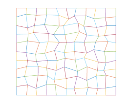
(a) $n=1$;

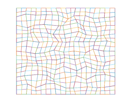
(b) $n=2$;

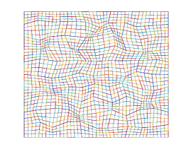
(c) $n=3$.

Figure 6.1. Non-uniform quadrilateral meshes.

Approximation errors in $L^{2}$-, $H(\text{curl})$- and $H(\text{curl}^{2})$-seminorms, i.e., $\|\bm{e}_{N}^{h}\|$, $\|\nabla\times\bm{e}_{N}^{h}\|$ and $\|\nabla\times\nabla\times\bm{e}_{N}^{h}\|$, are obtained in Table 6.1 and Table 6.2 for $N=1$ and $N=2$, respectively.

With the approximation space $\overset{\scriptscriptstyle\circ}{W}{}_{1}^{h}$, the simplest $H(\text{curl}^{2})$-conforming quadrilateral method consists 8 DOFs on each physical element. The vector field $\bm{u}_{1}^{h}$ converges to $\bm{u}$ at orders of $\mathcal{O}(h)$, $\mathcal{O}(h^{2})$ and $\mathcal{O}(h)$ in semi-norms in $L^{2}(\Omega)$, $H(\text{curl};\Omega)$ and $H(\text{curl}^{2};\Omega)$, respectively. This situation agrees well with the convergence behavior of the simplest rectangular elements reported in [11].

Table 6.1. Numerical results by using $H(\text{curl}^{2})$-conforming elements with $L=M=N=1$.

$h$	$\left\|\bm{e}_{1}^{h}\right\|$	rates	$\left\|\nabla\times\bm{e}_{1}^{h}\right\|$	rates	$\left\|\nabla\times\nabla\times\bm{e}_{1}^{h}\right\|$	rates
$1/10$	2.7016060e-01		8.9911798e-01		31.9663395
$1/20$	1.3087910e-01	1.0456	1.9697265e-01	2.1905	14.7861071	1.1123
$1/40$	6.5062865e-02	1.0083	4.7352656e-02	2.0565	7.23589118	1.0310
$1/80$	3.2494568e-02	1.0016	1.1725121e-02	2.0138	3.59895334	1.0076
$1/160$	1.6243391e-02	1.0003	2.9243540e-03	2.0034	1.79714478	1.0019

Note that the convergence rate of $\bm{u}_{1}^{h}$ is lower than that of $\nabla\times\bm{u}_{1}^{h}$. This is very different from convergence behaviors of elliptic equations with the gradient operator.

In order to improves the rate of convergence for $\bm{u}_{1}^{h}$, more DOFs are needed. So we carry out numerical experiments on the $H(\text{curl}^{2})$-conforming quadrilateral method with the approximation space $\overset{\scriptscriptstyle\circ}{W}{}_{2}^{h}$. We see from Table 6.2 that with 13 element DOFs ($L=M=N=2$), the convergence rate of $\bm{u}_{2}^{h}$ raises to $O(h^{2})$, while the convergence rates (even accuracy) of $\nabla\times\bm{u}_{2}^{h}$ and $\nabla\times\nabla\times\bm{u}_{2}^{h}$ are unchanged.

Table 6.2. Numerical results by using $H(\text{curl}^{2})$-conforming quadrilateral elements with $L=M=N=2$.

$h$	$\left\|\bm{e}_{2}^{h}\right\|$	rates	$\left\|\nabla\times\bm{e}_{2}^{h}\right\|$	rates	$\left\|\nabla\times\nabla\times\bm{e}_{2}^{h}\right\|$	rates
$1/10$	9.1992742e-02		8.7767063e-01		31.8557504
$1/20$	2.0157951e-02	2.1902	1.9253484e-01	2.1886	14.7330986	1.1125
$1/40$	4.8913038e-03	2.0431	4.6475991e-02	2.0506	7.21785897	1.0294
$1/80$	1.2142849e-03	2.0101	1.1519875e-02	2.0124	3.59091342	1.0072
$1/160$	3.0305706e-04	2.0024	2.8738828e-03	2.0031	1.79323838	1.0018

Whenever $K$ becomes a rectangle, the DOFs reduces to 12, which is one DOF less than the rectangular element in [11].

Next, let us examine the $h$-convergence of $\bm{u}_{L,M,N}^{h}$ with $L=N=3$ and $M=N,N+1$. Table 6.3 and Table 6.4 show that the errors $\|\bm{e}_{N,M,N}^{h}\|$, $\|\nabla\times\bm{e}_{N,M,N}^{h}\|$ and $\|\nabla\times\nabla\times\bm{e}_{N,M,N}^{h}\|$ decay asymptotically as $\mathcal{O}(h^{M})$, $\mathcal{O}(h^{N})$ and $\mathcal{O}(h^{N-1})$, respectively. It implies that the convergence order in the $L^{2}$-norm will increase by one if one supplements 4 DOFs on each element to change the approximation space $\overset{\scriptscriptstyle\circ}{W}{}^{h}_{N,N,N}$ to $\overset{\scriptscriptstyle\circ}{W}{}^{h}_{N,N+1,N}$. Similar convergence behavior of $\bm{u}_{N,M,N}^{h}$ can be observed in Table 6.5 and Table 6.6 for $L=N=4$ and $M=N,N+1$.

Table 6.3. Numerical results by using the $H(\text{curl}^{2})$-conforming elements with $L=M=N=3$.

$h$	$\left\|\bm{e}_{3}^{h}\right\|$	rates	$\left\|\nabla\times\bm{e}_{3}^{h}\right\|$	rates	$\left\|\nabla\times\nabla\times\bm{e}_{3}^{h}\right\|$	rates
$1/10$	1.4531621e-02		2.356674e-01		1.3413460e+01
$1/20$	1.1122290e-03	3.7076	2.875953e-02	3.0346	3.6870789e+00	1.8631
$1/40$	8.3518345e-05	3.7352	3.672498e-03	2.9692	9.7564651e-01	1.9180
$1/80$	6.6964145e-06	3.6406	4.640792e-04	2.9843	2.5019086e-01	1.9633
$1/160$	6.4506166e-07	3.3759	5.825095e-05	2.9940	6.3218033e-02	1.9846

Table 6.4. Numerical results by using the $H(\text{curl}^{2})$-conforming elements with $M=4,\ L=N=3$.

$h$	$\left\|\bm{e}_{3,4,3}^{h}\right\|$	rates	$\left\|\nabla\times\bm{e}_{3,4,3}^{h}\right\|$	rates	$\left\|\nabla\times\nabla\times\bm{e}_{3,4,3}^{h}\right\|$	rates
$1/10$	1.4367808e-02		2.3566738e-01		1.3413460e+01
$1/20$	1.0749797e-03	3.7405	2.8759528e-02	3.0346	3.6870789e+00	1.8631
$1/40$	7.5421333e-05	3.8332	3.6724978e-03	2.9692	9.7564651e-01	1.9180
$1/80$	4.9693459e-06	3.9238	4.6407944e-04	2.9843	2.5019086e-01	1.9633

Table 6.5. Numerical results by using the $H(\text{curl}^{2})$-conforming elements with $L=M=N=4$.

$h$	$\left\|\bm{e}_{4}^{h}\right\|$	rates	$\left\|\nabla\times\bm{e}_{4}^{h}\right\|$	rates	$\left\|\nabla\times\nabla\times\bm{e}_{4}^{h}\right\|$	rates
$1/10$	3.5791271e-04		1.4638912e-02		1.3023272
$1/20$	1.6019024e-05	4.4817	9.5069288e-04	3.9447	1.6959892e-01	2.9409
$1/40$	8.6362784e-07	4.2132	5.9743054e-05	3.9921	2.1604928e-02	2.9727
$1/80$	5.1620409e-08	4.0644	3.7288683e-06	4.0020	2.7236022e-03	2.9878

Table 6.6. Numerical results by using the $H(\text{curl}^{2})$-conforming elements with $M=5,L=N=4$.

$h$	$\left\|\bm{e}_{4,5,4}^{h}\right\|$	rates	$\left\|\nabla\times\bm{e}_{4,5,4}^{h}\right\|$	rates	$\left\|\nabla\times\nabla\times\bm{e}_{4,5,4}^{h}\right\|$	rates
$1/10$	1.8193533e-04		1.0483422e-02		9.1705319e-01
$1/20$	5.7613686e-06	4.9809	6.6294347e-04	3.9831	1.1567122e-01	2.9870
$1/40$	1.8301771e-07	4.9764	4.1611226e-05	3.9938	1.4503254e-02	2.9956
$1/80$	5.7630487e-09	4.9890	2.6033668e-06	3.9985	1.8134660e-03	2.9996

We point out that our $H(\operatorname{curl}^{2})$-conforming elements outperform the ones designed in [11], since our method using approximation spaces $\overset{\scriptscriptstyle\circ}{W}{}_{N,N+1,N}^{h}$ ($N\geq 3$) with $2N^{2}+2N+4$ DOFs on each quadrilateral element provides convergence orders $\mathcal{O}(h^{N+1})$ in $L^{2}(\Omega)$, $\mathcal{O}(h^{N})$ in $H(\text{curl};\Omega)$ and $\mathcal{O}(h^{N-1})$ in $H(\text{curl}^{2};\Omega)$ for the numerical vector field, while [11] needs $2N^{2}+4N+3$ DOFs on each rectangular element to acquire the same orders of convergence.

Interestingly, the situation where the convergence rate of $\bm{u}_{L,M,N}^{h}$ is lower than that of $\nabla\times\bm{u}_{L,M,N}^{h}$ can be reproduced for any $L=N-1,M=N-1$ with $N\geq 4$. Indeed, Table 6.7 shows that the errors $\|\bm{e}_{N-1,N-1,N}^{h}\|$, $\|\nabla\times\bm{e}_{N-1,N-1,N}^{h}\|$ and $\|\nabla\times\nabla\times\bm{e}_{N-1,N-1,N}^{h}\|$ decay asymptotically as $\mathcal{O}(h^{N-1})$, $\mathcal{O}(h^{N})$ and $\mathcal{O}(h^{N-1})$, respectively.

Table 6.7. Numerical results by using the $H(\text{curl}^{2})$-conforming elements with $L=M=3,N=4$.

$h$	$\left\|\bm{e}_{3,3,4}^{h}\right\|$	rates	$\left\|\nabla\times\bm{e}_{3,3,4}^{h}\right\|$	rates	$\left\|\nabla\times\nabla\times\bm{e}_{3,3,4}^{h}\right\|$	rates
$1/10$	1.7929703e-03		5.9958211e-03		5.6265349e-01
$1/20$	2.2577801e-04	2.9894	3.8206331e-04	3.9721	7.1249756e-02	2.9813
$1/40$	2.8439099e-05	2.9890	2.4014441e-05	3.9918	8.9231314e-03	2.9973
$1/80$	3.5631885e-06	2.9966	1.5037520e-06	3.9973	1.1151661e-03	3.0003

To test the $p$-convergence of our method, we set $L=M=N$ and let (a) $h=1$ for one element, (b) $h=1/2$ for 4 elements, (c) $h=1/8$ for 64 elements. Numerical errors versus various DOFs are shown in Figure 6.2 in a semi-logrithm scale. Three plots in Figure 6.2 demonstrate the exponential orders of convergence of our $H(\operatorname{curl}^{2})$-conforming quadrilateral spectral element method. It is noted that $h=1$ provides the optimal convergence rate, and an obvious decrease in the convergence rate is observed as the total number of elements increases. Moreover, for fixed DOFs, the accuracy decrease monotonously as $h$ decreases and thus $h=1$ offers the highest accuracy.

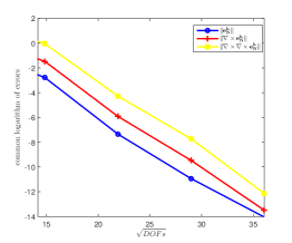
(a) $h=1$ for single element;

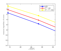
(b) $h=1/2$ for 4 elements;

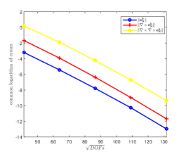
(c) $h=1/8$ for 64 elements.

Figure 6.2. The $\bm{L}^{2}$-errors of $\bm{u},\nabla\times\bm{u}$ and $(\nabla\times)^{2}\bm{u}$ versus $\sqrt{DOFs}$ in semi-log scale by using the $H(\text{curl}^{2})$-conforming quadrilateral spectral elements.

6.2. The quad-curl eigenvalue problem

We propose the quadrilateral spectral element method to solve the quad-curl eigenvalue problem which just substitutes $\lambda\bm{u}$ for the right-hand term $\bm{f}$ of the source problem (5.2).

As we have seen from Subsection 6.1, the selection of $L$ and $M$ affects the convergence rate for $\boldsymbol{u}$ only. On the other hand, the accuracy of eigenvalue approximation has much to do with accuracy of computed $\nabla\times\nabla\times\boldsymbol{u}$. Hence, in this subsection, we always choose $L=M=N$.

The approximation scheme for the eigenvalue problem is to find $\lambda_{N}^{h}\in\mathbb{R}$ and $(\bm{u}_{N}^{h},p_{N}^{h})\in\overset{\scriptscriptstyle\circ}{W}{}_{N}^{h}\times\overset{\scriptscriptstyle\circ}{S}{}_{N}^{h}$, s.t.

(6.2) $$\begin{cases}\displaystyle a(\bm{u}_{N}^{h},\bm{v}_{N}^{h})+b(\bm{v}_{N}^{h},p_{N}^{h})=\lambda_{N}^{h}(\bm{u}_{N}^{h},\bm{v}_{N}^{h}),&\forall\bm{v}_{N}^{h}\in\overset{\scriptscriptstyle\circ}{W}{}_{N}^{h},\\ \displaystyle b(\bm{u}_{N}^{h},q_{N}^{h})=0,&\forall q_{N}^{h}\in\overset{\scriptscriptstyle\circ}{S}{}_{N}^{h}.\end{cases}$$

6.2.1. Square domain

Denote by $\lambda_{i}$ the $i$-th exact eigenvalue and by $\lambda_{N,i}^{h}$ the $i$-th numerical eigenvalue. We demonstrate convergence orders of the first five discrete eigenvalues with various mesh sizes by using the simplest $H(\operatorname{curl}^{2})$-conforming quadrilateral elements in Table 6.8. Relative errors are then plotted in Figure 6.3 (a). Second-order $h$-convergence can be observed in both Table 6.8 and Figure 6.3 (a) for each discrete eigenvalue. Noting that an eigenvalue converges twice as fast as its eigenfunction, we confirm that the convergence orders of the simplest $H(\operatorname{curl}^{2})$-conforming quadrilateral element method for the eigenvalue problem are consistent with those for the source problem reported in the last subsection.

Table 6.8. The first 5 quad-curl eigenvalues on $[0,1]^{2}$ and their convergence orders by using $H(\text{curl}^{2})$-conforming quadrilateral elements with $N=1$.

$h$	$\lambda_{1,1}^{h}$	order	$\lambda_{1,2}^{h}$	order	$\lambda_{1,3}^{h}$	order	$\lambda_{1,4}^{h}$	order	$\lambda_{1,5}^{h}$	order
$1/5$	761.635	-	764.313	-	2437.229	-	5063.90	-	6097.93	-
$1/10$	720.783	2.06	721.198	2.09	2370.70	2.03	4433.19	2.16	5250.20	2.25
$1/20$	711.142	2.01	711.241	2.02	2355.17	1.99	4298.94	2.04	5078.26	2.06
$1/40$	708.763	2.00	708.787	2.00	2351.29	1.99	4266.53	2.01	5037.42	2.01
$1/80$	708.169	-	708.175	-	2350.31	-	4258.49	-	5027.34	-

Table 6.9. The first 5 quad-curl eigenvalues on $[0,1]^{2}$ and their convergence orders by using the $H(\text{curl}^{2})$-conforming elements with $N=3$.

$h$	$\lambda^{h}_{3,1}$	order	$\lambda^{h}_{3,2}$	order	$\lambda^{h}_{3,3}$	order	$\lambda^{h}_{3,4}$	order	$\lambda^{h}_{3,5}$	order
$1/5$	710.200	-	711.203	-	2364.96	-	4308.39	-	5078.35	-
$1/10$	708.139	3.72	708.207	3.77	2351.22	3.58	4259.70	3.75	5027.69	3.87
$1/20$	707.983	3.82	707.987	3.84	2350.07	3.75	4256.08	3.84	5024.23	3.95
$1/40$	707.972	3.86	707.972	3.87	2349.99	3.82	4255.83	3.88	5024.00	3.98
$1/80$	707.971	-	707.971	-	2349.98	-	4255.81	-	5023.99	-

Table 6.10. The first 5 quad-curl eigenvalues on $[0,1]^{2}$ and their convergence orders by using the $H(\text{curl}^{2})$-conforming elements with $N=4$.

$h$	$\lambda^{h}_{4,1}$	order	$\lambda^{h}_{4,2}$	order	$\lambda^{h}_{4,3}$	order	$\lambda^{h}_{4,4}$	order	$\lambda^{h}_{4,5}$	order
$1/5$	708.0004	-	708.0034	-	2350.2475	-	4256.8267	-	5024.7537	-
$1/10$	707.9731	4.20	707.9732	4.29	2350.0016	4.05	4255.8534	4.71	5024.0055	5.85
$1/20$	707.9716	4.07	707.9716	4.10	2349.9868	4.06	4255.8162	4.30	5023.9926	5.95
$1/40$	707.9715	3.93	707.9715	4.19	2349.9859	4.06	4255.8143	4.09	5023.9923	6.40
$1/80$	707.9715	-	707.9715	-	2349.9859	-	4255.8142	-	5023.9923	-

Further, let us set $h=1/5$ as the initial mesh size and carry out numerical experiments on the $h$-version of the $H(\operatorname{curl}^{2})$-conforming quadrilateral elements for (6.2) with $N=3,4$. The first five discrete eigenvalues are shown in Table 6.9 for $N=3$ and Table 6.10 for $N=4$, and their relative errors are depicted in Figure 6.3 (b) and (c). From these tables and figures, one readily finds that all five discrete eigenvalues converge at the full order around $4$ for $N=3$. At the same time, only the fifth discrete eigenvalue converges at the full order around $6$, while the first four eigenfunctions have still a convergence order slightly larger than $4$ owing to the limited regularity of their eigenfunctions.

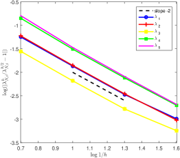
(a) $N=1$;

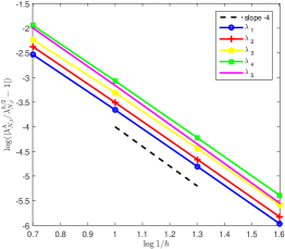
(b) $N=3$;

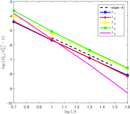
(c) $N=4$.

Figure 6.3. Eigenvalue errors versus $h$ for the first five eigenvalues on $[0,1]^{2}$.

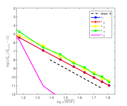
(a) $h=1$;

(b) $h=1/2$;

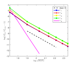
(c) $h=1/10$.

Figure 6.4. Eigenvalue errors versus $\sqrt{DOFs}$ of the $H(\text{curl}^{2})$-conforming quadrilateral spectral method on $[0,1]^{2}$.

Next, we let (a) $h=1$ for one element, (b) $h=1/2$ for 4 elements, (c) $h=1/10$ for 100 elements, then examine the $p$-convergence of our $H(\operatorname{curl}^{2})$-conforming quadrilateral elements. Errors of numerical eigenvalues versus various DOFs are plotted in Figure 6.4 in log-log scale. Distinct to those for infinitely smooth problems, our $H(\operatorname{curl}^{2})$-conforming quadrilateral spectral element methods for quad-curl eigenvalue problems only have algebraic orders of convergence. Indeed, the quad-curl eigenvalue problem is essentially a sixth order partial differential equation, and singularities shall occur even on a square domain, so that only limited convergence orders can be obtained in both the $p$- and $h$-versions of our method. Nevertheless, the convergence rates for a fixed eigenvalue are independent of the total number of elements used in our $p$-version spectral element methods. Indeed, they are twice as high as those of the $h$-version for $N\geq 4$.

6.2.2. L-shaped domain

The quad-curl eigenvalue problem on an L-shaped domain $\Omega=(0,1)\times(0,1)/[0.5,1)\times[0.5,1)$ is also considered. Due to the strong singularity of the domain, convergence rate for the first eigenvalue deteriorates to around $h^{4/3}$ in the $h$-version (see Table 6.2.2). While, it is observed that the convergence rate in the $p$-version with $h=1/6$ is nearly $N^{-3.5}$ (see Figure 6.5). Once again, these reflect the correctness and efficiency of our $H(\text{curl}^{2})$-conforming quadrilateral spectral element method.

Table 6.11. The first quad-curl eigenvalue and the convergence order by $H(\operatorname{curl}^{2})$-conforming quadrilateral spectral elements with $N=4$ on the L-shaped domain.

$h$	$\lambda^{h}_{4,1}$	error	order
$1/4$	534.46527767676	8.920012568e-04	-
$1/8$	534.94202137614	4.411857535e-04	1.0156
$1/16$	535.17803017493	1.814911829e-04	1.2815
$1/32$	535.27516026869	7.262977955e-05	1.3213
$1/64$	535.31403718558	2.889401638e-05	1.3298
$1/128$	535.32950455814	-	-

Figure 6.5. Eigenvalue errors versus $N$ of the $H(\operatorname{curl}^{2})$-conforming quadrilateral spectral element method on the L-shape domain.

7. Conclusion

In this paper, we have constructed $H(\text{curl}^{2})$-conforming basis functions on an arbitrary convex quadrilateral element using the bilinear mapping from the reference square onto the physical element together with the contravariant transformation of vector fileds. These hierarchical basis functions are explicitly formulated in generalized Jacobi polynomials with the indices of $(-1,-1)$ and $(-2,-2)$, which are easier to generalize to higher order approximation scheme than the Lagrangian bases [29]. Numerical results show that our $H(\text{curl}^{2})$-conforming spectral elements are efficient and can achieve an exponential order of $p$-convergence and an optimal order, $\mathcal{O}(h^{N-1})$, of $h$-convergence for source problems measured in the $H(\text{curl}^{2};\Omega)$-norm. However, owing to the strong singularities, our $H(\text{curl}^{2})$-conforming spectral elements get only limited orders of convergence in both the $p$- and $h$-versions for eigenvalue problems.

Appendix A Proof of Lemma 5.1

$Proof\ of\ Lemma\ \emph{\ref{lowerorderpolynomials}}.$ Based on (3.10), (3.11), (3.12), and, (3.13), one can obtain

$$-x_{14}\hat{\bm{\phi}}_{0,0}+x_{21}\hat{\bm{\phi}}_{1,0}+x_{32}\hat{\bm{\phi}}_{1,1}-x_{43}\hat{\bm{\phi}}_{0,1}$$

$$= \left(\frac{x_{21}+x_{34}}{4}+\frac{-x_{21}+x_{34}}{4}\hat{y},\frac{x_{41}+x_{32}}{4}+\frac{-x_{41}+x_{32}}{4}\hat{x}\right)^{\mathsf{T}}$$

$$= B_{K}^{\mathsf{T}}(1,0)^{\mathsf{T}},$$

which implies (5.4). Similarly, (5.5) can be yielded.

Furthermore, we also have

(A.1) $$\begin{split}&-\frac{(x_{1}^{2}-x_{4}^{2})}{2}\hat{\bm{\phi}}_{0,0}+\frac{(x_{2}^{2}-x_{1}^{2})}{2}\hat{\bm{\phi}}_{1,0}+\frac{(x_{3}^{2}-x_{2}^{2})}{2}\hat{\bm{\phi}}_{1,1}-\frac{(x_{4}^{2}-x_{3}^{2})}{2}\hat{\bm{\phi}}_{0,1}\\ =&\Big{(}\frac{(x_{1}^{2}-x_{2}^{2}+x_{3}^{2}-x_{4}^{2})\hat{y}}{8}+\frac{-x_{1}^{2}+x_{2}^{2}+x_{3}^{2}-x_{4}^{2}}{8},\\ &\frac{(x_{1}^{2}-x_{2}^{2}+x_{3}^{2}-x_{4}^{2})\hat{x}}{8}+\frac{-x_{1}^{2}-x_{2}^{2}+x_{3}^{2}+x_{4}^{2}}{8}\Big{)}^{\mathsf{T}}.\end{split}$$

By (3.10)-(3.13), one finds

(A.2) $$\begin{split}&\frac{x_{14}^{2}}{2}\hat{\bm{\phi}}_{0,2}+\frac{x_{21}^{2}}{2}\hat{\bm{\phi}}_{2,0}+\frac{x_{32}^{2}}{2}\hat{\bm{\phi}}_{1,2}+\frac{x_{43}^{2}}{2}\hat{\bm{\phi}}_{2,1}\\ =&\Bigg{(}-\frac{x_{41}^{2}(\hat{y}^{2}-1)}{16}+\frac{x_{21}^{2}\hat{x}(1-\hat{y})}{8}+\frac{x_{32}^{2}(\hat{y}^{2}-1)}{16}+\frac{x_{43}^{2}\hat{x}(1+\hat{y})}{8},\\ &\frac{x_{41}^{2}(1-\hat{x})\hat{y}}{8}-\frac{x_{21}^{2}(\hat{x}^{2}-1)}{16}+\frac{x_{32}^{2}(1+\hat{x})\hat{y}}{8}+\frac{x_{43}^{2}(\hat{x}^{2}-1)}{16}\Bigg{)}^{\mathsf{T}},\end{split}$$

and

(A.3) $$\begin{split}&\frac{(x_{32}+x_{14})^{2}}{2}\hat{\bm{\phi}}_{2,2}\\ =&\Bigg{(}\frac{(x_{32}+x_{14})^{2}\hat{x}(\hat{y}^{2}-1)}{16},\frac{(x_{32}+x_{14})^{2}(\hat{x}^{2}-1)\hat{y}}{16}\Bigg{)}^{\mathsf{T}}.\end{split}$$

Adding (A.1)-(A.3) up, then

$$-\frac{(x_{1}^{2}-x_{4}^{2})}{2}\hat{\bm{\phi}}_{0,0}+\frac{(x_{2}^{2}-x_{1}^{2})}{2}\hat{\bm{\phi}}_{1,0}+\frac{(x_{3}^{2}-x_{2}^{2})}{2}\hat{\bm{\phi}}_{1,1}-\frac{(x_{4}^{2}-x_{3}^{2})}{2}\hat{\bm{\phi}}_{0,1}+\frac{x_{14}^{2}}{2}\hat{\bm{\phi}}_{0,2}$$

$$+\frac{x_{21}^{2}}{2}\hat{\bm{\phi}}_{2,0}+\frac{x_{32}^{2}}{2}\hat{\bm{\phi}}_{1,2}+\frac{x_{43}^{2}}{2}\hat{\bm{\phi}}_{2,1}+\frac{(x_{32}+x_{14})^{2}}{2}\hat{\bm{\phi}}_{2,2}$$

$$= \Bigg{(}\left(\frac{x_{21}}{2}\frac{1-\hat{y}}{2}+\frac{x_{34}}{2}\frac{1+\hat{y}}{2}\right)\left(\sigma_{1}(\hat{x},\hat{y})x_{1}+\sigma_{2}(\hat{x},\hat{y})x_{2}+\sigma_{3}(\hat{x},\hat{y})x_{3}+\sigma_{4}(\hat{x},\hat{y})x_{4}\right),$$

$$\left(\frac{x_{41}}{2}\frac{1-\hat{x}}{2}+\frac{x_{32}}{2}\frac{1+\hat{x}}{2}\right)\left(\sigma_{1}(\hat{x},\hat{y})x_{1}+\sigma_{2}(\hat{x},\hat{y})x_{2}+\sigma_{3}(\hat{x},\hat{y})x_{3}+\sigma_{4}(\hat{x},\hat{y})x_{4}\right)\Bigg{)}^{\mathsf{T}}$$

$$= B_{K}^{\mathsf{T}}(x,0)^{\mathsf{T}}.$$

Hence, we arrive at (5.6). If analyzing a bit, we can find (5.8).

Now, let us prove (5.7) and (5.9). Some equations are calculated as follows:

$$-\frac{(x_{1}+x_{4})y_{14}}{2}\hat{\bm{\phi}}_{0,0}+\frac{(x_{2}+x_{1})y_{21}}{2}\hat{\bm{\phi}}_{1,0}+\frac{(x_{3}+x_{2})y_{32}}{2}\hat{\bm{\phi}}_{1,1}-\frac{(x_{4}+x_{3})y_{43}}{2}\hat{\bm{\phi}}_{0,1}$$

$$= \Bigg{(}\frac{y_{42}x_{13}-y_{13}x_{42}}{64}\hat{y}(\hat{y}^{2}-1)(3\hat{x}^{2}-5)+\frac{(x_{2}+x_{1})y_{21}}{8}(1-\hat{y})-\frac{(x_{4}+x_{3})y_{43}}{8}(1+\hat{y}),$$

(A.4) $$\frac{y_{24}x_{13}-y_{13}x_{24}}{64}\hat{x}(\hat{x}^{2}-1)(3\hat{y}^{2}-5)+\frac{(x_{4}+x_{1})y_{41}}{8}(1-\hat{x})-\frac{(x_{2}+x_{3})y_{23}}{8}(1+\hat{x})\Bigg{)}^{\mathsf{T}},$$

$$\frac{x_{14}y_{14}}{2}\hat{\bm{\phi}}_{0,2}+\frac{x_{21}y_{21}}{2}\hat{\bm{\phi}}_{2,0}+\frac{x_{32}y_{32}}{2}\hat{\bm{\phi}}_{1,2}+\frac{x_{43}y_{43}}{2}\hat{\bm{\phi}}_{2,1}$$

$$= \Bigg{(}-\frac{x_{41}y_{41}(\hat{y}^{2}-1)}{16}+\frac{x_{21}y_{21}\hat{x}(1-\hat{y})}{8}+\frac{x_{32}y_{32}(\hat{y}^{2}-1)}{16}+\frac{x_{43}y_{43}\hat{x}(1+\hat{y})}{8},$$

(A.5) $$\frac{x_{41}y_{41}(1-\hat{x})\hat{y}}{8}-\frac{x_{21}y_{21}(\hat{x}^{2}-1)}{16}+\frac{x_{32}y_{32}(1+\hat{x})\hat{y}}{8}+\frac{x_{43}y_{43}(\hat{x}^{2}-1)}{16}\Bigg{)}^{\mathsf{T}},$$

and,

$$\frac{(x_{32}+x_{14})(y_{32}+y_{14})}{2}\hat{\bm{\phi}}_{2,2}$$

(A.6) $$= \Bigg{(}\frac{(x_{32}+x_{14})(y_{32}+y_{14})}{4}\frac{\hat{y}^{2}-1}{4}\hat{x},\frac{(x_{32}+x_{14})(y_{32}+y_{14})}{4}\frac{\hat{x}^{2}-1}{4}\hat{y}\Bigg{)}^{\mathsf{T}}.$$

Replacing $l_{i},s_{i}$ with $x_{i},y_{i},i=1,\cdots,4$, one can arrive at

$$\hat{\bm{\psi}}_{0,0}+\hat{\bm{\psi}}_{0,1}+\hat{\bm{\psi}}_{1,0}+\hat{\bm{\psi}}_{1,1}$$

$$= \Bigg{(}\frac{3(1-\hat{y})(1+\hat{y})}{64}\Big{(}(y_{42}x_{13}-y_{13}x_{42})(\hat{x}^{2}-\frac{5}{3})\hat{y}+\frac{4}{3}(y_{32}x_{14}-y_{14}x_{32})\Big{)},$$

(A.7) $$\frac{3(\hat{x}-1)(1+\hat{x})}{64}\Big{(}(y_{42}x_{13}-y_{13}x_{42})(\hat{y}^{2}-\frac{5}{3})\hat{x}+\frac{4}{3}(y_{43}x_{12}-y_{12}x_{43})\Big{)}\Bigg{)}^{\mathsf{T}}.$$

Summing (A.4)-(A.7), it gives

$$-\frac{(x_{1}+x_{4})y_{14}}{2}\hat{\bm{\phi}}_{0,0}+\frac{(x_{2}+x_{1})y_{21}}{2}\hat{\bm{\phi}}_{1,0}+\frac{(x_{3}+x_{2})y_{32}}{2}\hat{\bm{\phi}}_{1,1}-\frac{(x_{4}+x_{3})y_{43}}{2}\hat{\bm{\phi}}_{0,1}$$

$$+\frac{x_{14}y_{14}}{2}\hat{\bm{\phi}}_{0,2}+\frac{x_{21}y_{21}}{2}\hat{\bm{\phi}}_{2,0}+\frac{x_{32}y_{32}}{2}\hat{\bm{\phi}}_{1,2}+\frac{x_{43}y_{43}}{2}\hat{\bm{\phi}}_{2,1}$$

$$+\frac{(x_{32}+x_{14})(y_{32}+y_{14})}{2}\hat{\bm{\phi}}_{2,2}+(\hat{\bm{\psi}}_{0,0}+\hat{\bm{\psi}}_{0,1}+\hat{\bm{\psi}}_{1,0}+\hat{\bm{\psi}}_{1,1})$$

$$= \Bigg{(}\left(\frac{y_{21}}{2}\frac{1-\hat{y}}{2}+\frac{y_{34}}{2}\frac{1+\hat{y}}{2}\right)\left(\sigma_{1}(\hat{x},\hat{y})x_{1}+\sigma_{2}(\hat{x},\hat{y})x_{2}+\sigma_{3}(\hat{x},\hat{y})x_{3}+\sigma_{4}(\hat{x},\hat{y})x_{4}\right),$$

$$\left(\frac{y_{41}}{2}\frac{1-\hat{x}}{2}+\frac{y_{32}}{2}\frac{1+\hat{x}}{2}\right)\left(\sigma_{1}(\hat{x},\hat{y})x_{1}+\sigma_{2}(\hat{x},\hat{y})x_{2}+\sigma_{3}(\hat{x},\hat{y})x_{3}+\sigma_{4}(\hat{x},\hat{y})x_{4}\right)\Bigg{)}^{\mathsf{T}}$$

$$= B_{K}^{\mathsf{T}}(0,x)^{\mathsf{T}},$$

which states (5.7). Similarly, we derive (5.9). (5.10) can be deduced from (5.7) since $\hat{\nabla}\times\hat{\bm{\bm{\phi}}}_{m,n}=0$, when $(m,n)\neq(i,j),\{i,j\}\in\{0,1\}$. Now we finish the proof.

References

- [1] D. Arnold. Finite Element Exterior Calculus. Society for Industrial and Applied Mathematics, Philadelphia, PA, 2018.
- [2] F. Ben Belgacem and C. Bernardi. Spectral element discretization of the Maxwell equations. Mathematics of Computation, 68(228):1497–1520, 1999.
- [3] S. C. Brenner, J. Cui, and L. Sung. Multigrid methods based on Hodge decomposition for a quad-curl problem. Computational Methods in Applied Mathematics, 19(2):215–232, 2019.
- [4] S. C. Brenner, J. Sun, and L. Sung. Hodge decomposition methods for a quad-curl problem on planar domains. Journal of Scientific Computing, 73(2-3):495–513, 2017.
- [5] W. Cai. Computational Methods for Electromagnetic Phenomena. Cambridge University Press, New York, 2013.
- [6] F. Cakoni and H. Haddar. A variational approach for the solution of the electromagnetic interior transmission problem for anisotropic media. Inverse Problems and Imaging, 1(3):443–456, 2017.
- [7] G. Cohen. Higher-Order numerical methods for transient wave equations. Springer-Verla, New York, 2002.
- [8] B. Guo, J. Shen, and L. Wang. Generalized jacobi polynomials/functions and their applications. Applied Numerical Mathematics, 59(5):1011–1028, 2009.
- [9] B. Guo and T. Wang. Composite Laguerre-Legendre spectral method for fourth-order exterior problems. Journal of Scientific Computing, 44(3):255–285, 2010.
- [10] Q. Hong, J. Hu, S. Shu, and J. Xu. A discontinuous Galerkin method for the fourth-order curl problem. Journal of Computational Mathematics, 30(6):565–578, 2012.
- [11] K Hu, Q. Zhang, and Z. Zhang. Simple curl-curl-conforming finite elements in two dimensions. arXiv, 2020.
- [12] H. Li, W. Shan, and Z. Zhang. -conforming quadrilateral spectral element method for fourth-order equations. Communications on Applied Mathematics and Computation, 1(3):403–434, 2019.
- [13] Y. Liu, J. Lee, X. Tian, and Q. Liu. A spectral-element time-domain solution of Maxwell’s equations. Microwave & Optical Technology Letters, 48(4):673–680, 2006.
- [14] P. Monk and J. Sun. Finite element methods for Maxwell’s transmission eigenvalues. SIAM Journal on Scientific Computing, 34(3):B247–B264, 2012.
- [15] L. Na, L. Tobón, Y. Zhao, Y. Tang, and Q. Liu. Mixed spectral-element method for 3-d Maxwell’s eigenvalue problem. IEEE Transactions on Microwave Theory & Techniques, 63(2):317–325, 2015.
- [16] S. Nicaise. Singularities of the quad curl problem. Journal of Differential Equations, 264(8):5025–5069, 2018.
- [17] A.T. Patera. A spectral element method for fluid dynamics: Laminar flow in a channel expansion. Journal of Computational Physics, 54(3):468–488, 1984.
- [18] J. Shen, L. Wang, and H. Li. A triangular spectral element method using fully tensorial rational basis functions. SIAM Journal on Numerical Analysis, 47(3):1619–1650, 2009.
- [19] J. Sun. A mixed FEM for the quad-curl eigenvalue problem. Numerische Mathematik, 132(1):185–200, 2016.
- [20] J. Sun and L. Xu. Computation of Maxwell’s transmission eigenvalues and its applications in inverse medium problems. Inverse Problems, 29(10):104013, 2013.
- [21] J. Sun, Q. Zhang, and Z. Zhang. A curl-conforming weak Galerkin method for the quad-curl problem. BIT Numerical Mathematics, 59:1093–1114, 2019.
- [22] J. Sun and A. Zhou. Finite Element Methods for Eigenvalue Problems. Chapman and Hall/CRC, Boca Raton, FL, 2016.
- [23] Z. Sun, J. Cui, F. Gao, and C. Wang. Multigrid methods for a quad-curl problem based on interior penalty method. Computers & Mathematics with Applications, 76(9):2192–2211, 2018.
- [24] G. Szeg. Orthogonal polynomials, volume 23. American Mathematical Society, 1939.
- [25] C. Wang, Z. Sun, and J. Cui. A new error analysis of a mixed finite element method for the quad-curl problem. Applied Mathematics and Computation, 349:23–38, 2019.
- [26] L. Wang, Q. Zhang, J. Sun, and Z. Zhang. A priori and a posteriori error estimates for the quad-curl eigenvalue problem. arXiv, 2020.
- [27] L. Wang, Q. Zhang, and Z. Zhang. Superconvergence analysis and PPR recovery of arbitrary order edge elements for maxwell’s equations. Journal of Scientific Computing, 78:1207–1230, 2019.
- [28] S. Zaglmayr. High Order Finite Element Methods for Electromagnetic Field Computation. PhD thesis, Graz University of Technology, 2006.
- [29] Q. Zhang, L. Wang, and Z. Zhang. H()-conforming finite elements in 2 dimensions and applications to the quad-curl problem. SIAM Journal on Scientific Computing, 41(3):A1527–A1547, 2019.
- [30] S. Zhang. Mixed schemes for quad-curl equations. Mathematical Modelling and Numerical Analysis, 52(1):147–161, 2018.
- [31] S. Zhang. Regular decomposition and a framework of order reduced methods for fourth order problems. Numerische Mathematik, 138(1):241–271, 2018.
- [32] B. Zheng and J. Xu. A nonconforming finite element method for fourth order curl equations in . Mathematics of Computation, 80(276):1871–1886, 2011.