Theory of Ca₁₀Cr₇O₂₈ as a bilayer breathing–kagome magnet:
Classical thermodynamics and semi–classical dynamics

Abstract

Ca₁₀Cr₇O₂₈ is a novel spin–$1/2$ magnet exhibiting spin liquid behaviour which sets it apart from any previously studied model or material. However, understanding Ca₁₀Cr₇O₂₈ presents a significant challenge, because the low symmetry of the crystal structure leads to very complex interactions, with up to seven inequivalent coupling parameters in the unit cell. Here we explore the origin of the spin-liquid behaviour in Ca₁₀Cr₇O₂₈, starting from the simplest microscopic model consistent with experiment — a Heisenberg model on a single bilayer of the breathing–kagome (BBK) lattice. We use a combination of classical Monte Carlo (MC) simulation and (semi–)classical Molecular Dynamics (MD) simulation to explore the thermodynamic and dynamic properties of this model, and compare these with experimental results for Ca₁₀Cr₇O₂₈. We uncover qualitatively different behaviours on different timescales, and argue that the ground state of Ca₁₀Cr₇O₂₈ is born out of a slowly-fluctuating “spiral spin liquid”, while faster fluctuations echo the U(1) spin liquid found in the kagome antiferromagnet. We also identify key differences between longitudinal and transverse spin excitations in applied magnetic field, and argue that these are a distinguishing feature of the spin liquid in the BBK model.

I Introduction

The search for quantum spin liquids (QSL), exotic phases which host new forms of magnetic excitations, has become one of the central themes of modern condensed matter physics Anderson (1973); Balents (2010); Savary and Balents (2016); Knolle and Moessner (2019). Fortunately, after a long “drought” Lee (2008), recent years have seen an explosion in the number of materials under study, with examples including quasi-2D organics Shimizu et al. (2003); Zhou et al. (2017), thin films of ³He Masutomi et al. (2004), spin–1/2 magnets with a kagome lattice Lee (2008); Han et al. (2012), “Kitaev” magnets with strongly anisotropic exchange Kitaev (2006); Jackeli and Khaliullin (2009); Banerjee et al. (2016); Baek et al. (2017); Winter et al. (2017); Hermanns et al. (2018), and quantum analogues of spin ice Hermele et al. (2004); Banerjee et al. (2008); Benton et al. (2012); Sibille et al. (2016); Benton et al. (2018). Another new arrival on this scene is the quasi–2D magnet Ca₁₀Cr₇O₂₈, a system which appears to have qualitatively different properties from any previously–studied spin liquid Balz et al. (2016, 2017a); Sonnenschein et al. (2019).

The first surprise in Ca₁₀Cr₇O₂₈ is a chemical one. Instead of the usual $3+$ valance, Cr ions exhibit a highly unusual, $5+$ valence Arcon et al. (1998). These Cr${}^{5^{+}}$ ions are magnetic, with spin S=1/2, and occupy sites of the breathing bilayer–kagome (BBK) lattice [Fig. 1] Balz et al. (2017b); Balodhi and Singh (2017). Curie–law fits to the magnetic susceptibility of Ca₁₀Cr₇O₂₈ reveal predominantly ferromagnetic (FM) interactions, with $\theta_{\sf CW}=2.35\ \text{K}$ Balz et al. (2016, 2017a). This is accompanied by a broad peak in heat capacity at about $T\approx 3.1\ \text{K}$ Balz et al. (2016, 2017a); Sonnenschein et al. (2019). However measurements of heat capacity, a.c. susceptibility and $\mu$SR asymmetry fail to find evidence of either, magnetic order, or spin–glass freezing, down to $19\ \text{mK}$, two orders of magnitude lower than the scale of interactions Balz et al. (2016). Consistent with this, neutron scattering experiments find no magnetic Bragg peaks down to $90\ \text{mK}$ Balz et al. (2016, 2017a); Sonnenschein et al. (2019). Instead, scattering is predominantly inelastic and highly–structured, with results at $0.25\ \text{meV}$ showing hints of a “ring” centered on (2,0,0), while scattering at intermediate and high energies suggests “bow–tie” like structures centered on (1,0,0) Balz et al. (2016, 2017a) [Fig. 2]. With the application of magnetic field, these structures evolve into relatively–sharp, dispersing excitations, with measurements of heat capacity suggesting a qualitative change in behaviour for fields $B\gtrsim 1T$ Balz et al. (2016, 2017a). This particular combination of dynamic and thermodynamic properties sets Ca₁₀Cr₇O₂₈ apart from any spin liquid material yet studied, and presents an interesting challenge to theory.

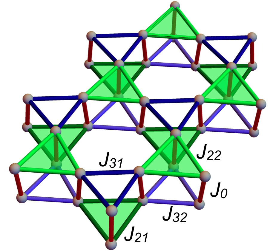
Figure 1: Bilayer breathing–Kagome (BBK) lattice realised by spin–1/2 Cr⁵⁺ ions in Ca₁₀Cr₇O₂₈. Interactions for the minimal spin–1/2 BBK model [Eq. (1)] are labelled following the conventions of Balz et al. Balz et al. (2016, 2017a). Experimental estimates of these parameters can be found in Table 2.

A range of different theoretical techniques have been applied to study Ca₁₀Cr₇O₂₈. Pseudo–fermion functional renormalisation group (PFFRG) calculations, for a spin–1/2 model parameterised from experiment, reproduce a “ring” in the static structure factor $S({\bf q},\omega=0)$, and suggest that the ground state of Ca₁₀Cr₇O₂₈ should be a quantum spin liquid Balz et al. (2016). This conclusion was supported by subsequent tensor–network calculations Kshetrimayum et al. (2020). Meanwhile the finite–temperature properties of Ca₁₀Cr₇O₂₈ have been explored through Monte Carlo simulations of a simplified, spin–3/2 honeycomb–lattice model Biswas and Damle (2018). At high temperatures, these also reveal “rings” in the equal–time structure factor $S({\bf q})$, while at low temperatures a 3–state Potts transition is found into a nematic state which breaks lattice–rotation symmetries, but lacks long–range magnetic order Mulder et al. (2010); Biswas and Damle (2018). And, intriguingly, the thermodynamic properties of Ca₁₀Cr₇O₂₈ have recently been argued to fit phenomenology based on spinons Sonnenschein et al. (2019).

None of these approaches, however, shed light on the nature of “bow–tie” structures observed at finite energies; the evolution of the spin liquid in magnetic field; or the finite–temperature properties of the microscopically relevant, spin–1/2 BBK model. And, most importantly, while there is agreement about the absence of conventional magnetic order, very little is known about the origins of the spin liquid which succeeds it.

This Article will be the first of two papers exploring the thermodynamics and dynamics of Ca₁₀Cr₇O₂₈, starting from the spin–1/2 BBK model proposed by Balz et al. Balz et al. (2016, 2017a)

$${\cal H}_{\sf BBK}=\sum_{\langle ij\rangle}J_{ij}{\bf S}_{i}\cdot{\bf S}_{j}-{\bf B}\cdot\sum_{i}{\bf S}_{i}\;,$$ (1)

where first–neighbour bonds $\langle ij\rangle$ are illustrated in Fig. 1, and parameters $J_{ij}$ can be extracted from fits to inelastic neutron scattering in high magnetic field $B\gg J$ [Table 2]. In this paper, we extend the results of an earlier preprint Pohle et al. (2017), making the approximation of treating spins as classical $O(3)$ vectors, and using a combination of classical Monte Carlo (MC) simulations and numerical integration of equations of motion (here referred to as “molecular dynamics” or “MD” simulation Moessner and Chalker (1998a)), to evaluate their dynamics. From this, we first establish a finite–temperature phase diagram for the BBK model of Ca₁₀Cr₇O₂₈, and then track the evolution of its properties as a function of energy and magnetic field. In the second Article, we will compare these findings with the results of exact diagonalization and finite–temperature quantum–typicality calculations for a spin–1/2 BBK model Shimokawa et al. (tion).

In the classical limit, considered in this Article, we find that the BBK model supports a spin liquid state for a wide range of temperatures and parameter values. At low energies, this is characterised by the slow, collective fluctuations of ferromagnetically aligned spins on triangular plaquettes. These give rise to a ring–like structure in the dynamical structure factor $S({\bf q},\omega)$, at low energies, while fluctuations at higher energies have a qualitatively different character, reflecting the Kagome–like physics of individual spin–1/2 moments. An added bonus of the (semi–)classical molecular dynamics simulations used is that both of these features can be visualised directly, through animations provided in the Supplemental Materials fir ; sec . At low temperatures, we find that this classical spin liquid undergoes a 3–state Potts transition into a phase breaking lattice–rotation symmetry (lattice nematic), consistent with results for an effective spin–3/2 model Biswas and Damle (2018). For parameters taken from experiment, this transition occurs at $T\approx 66\ \text{mK}$.

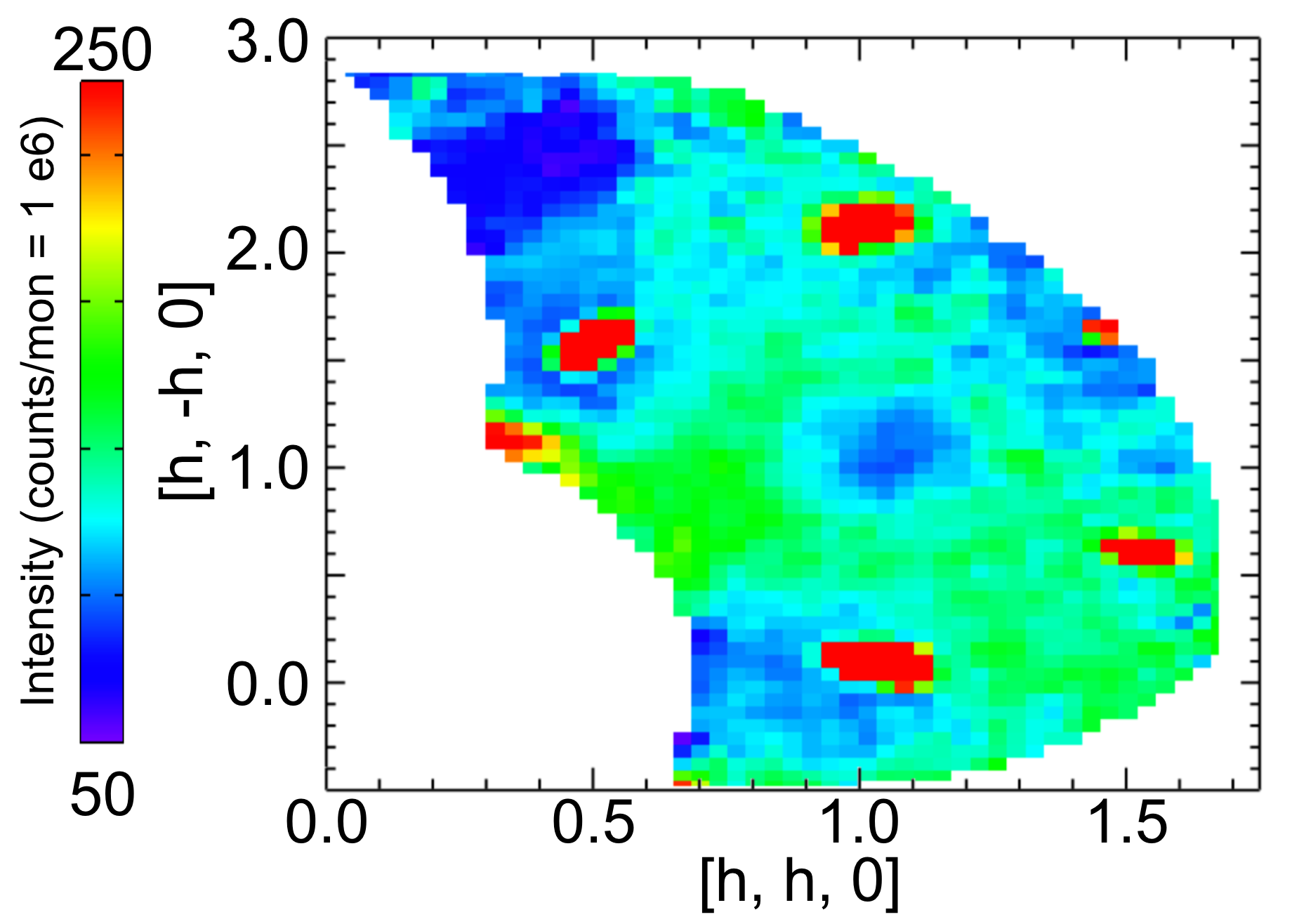
(a) (a) $E=$ 0.25 meV

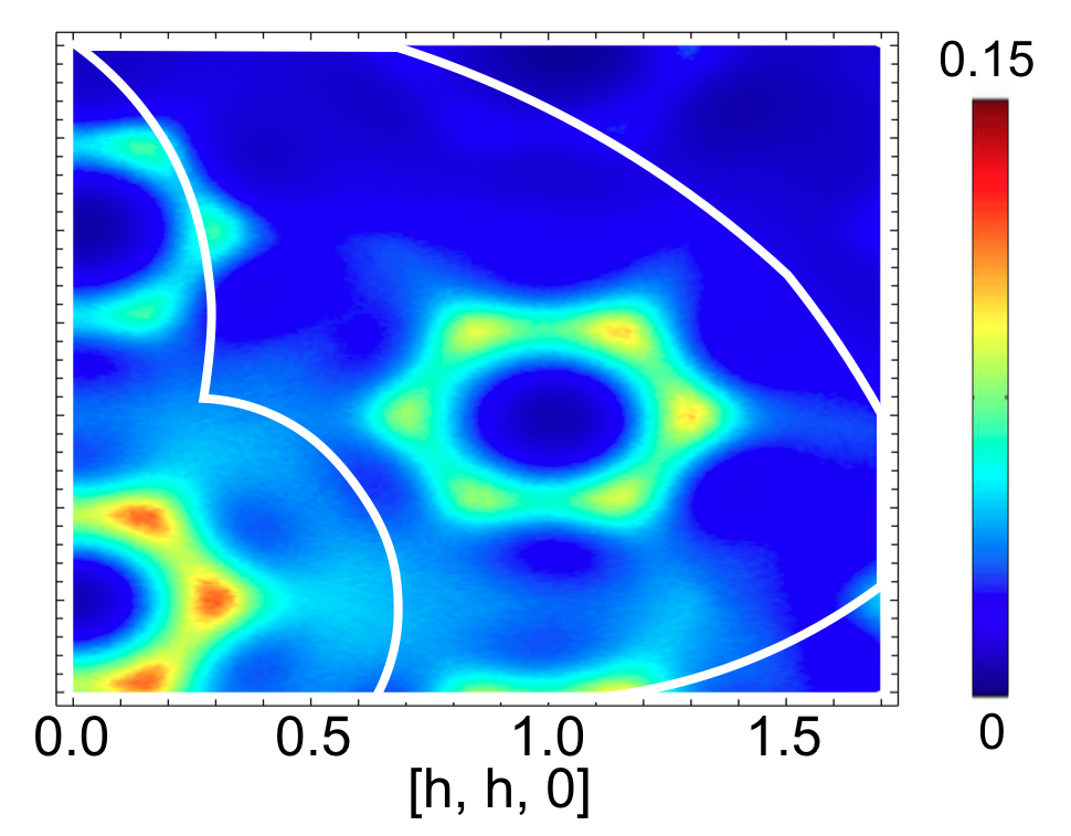
(b) (b) $E=$ 0.26 meV

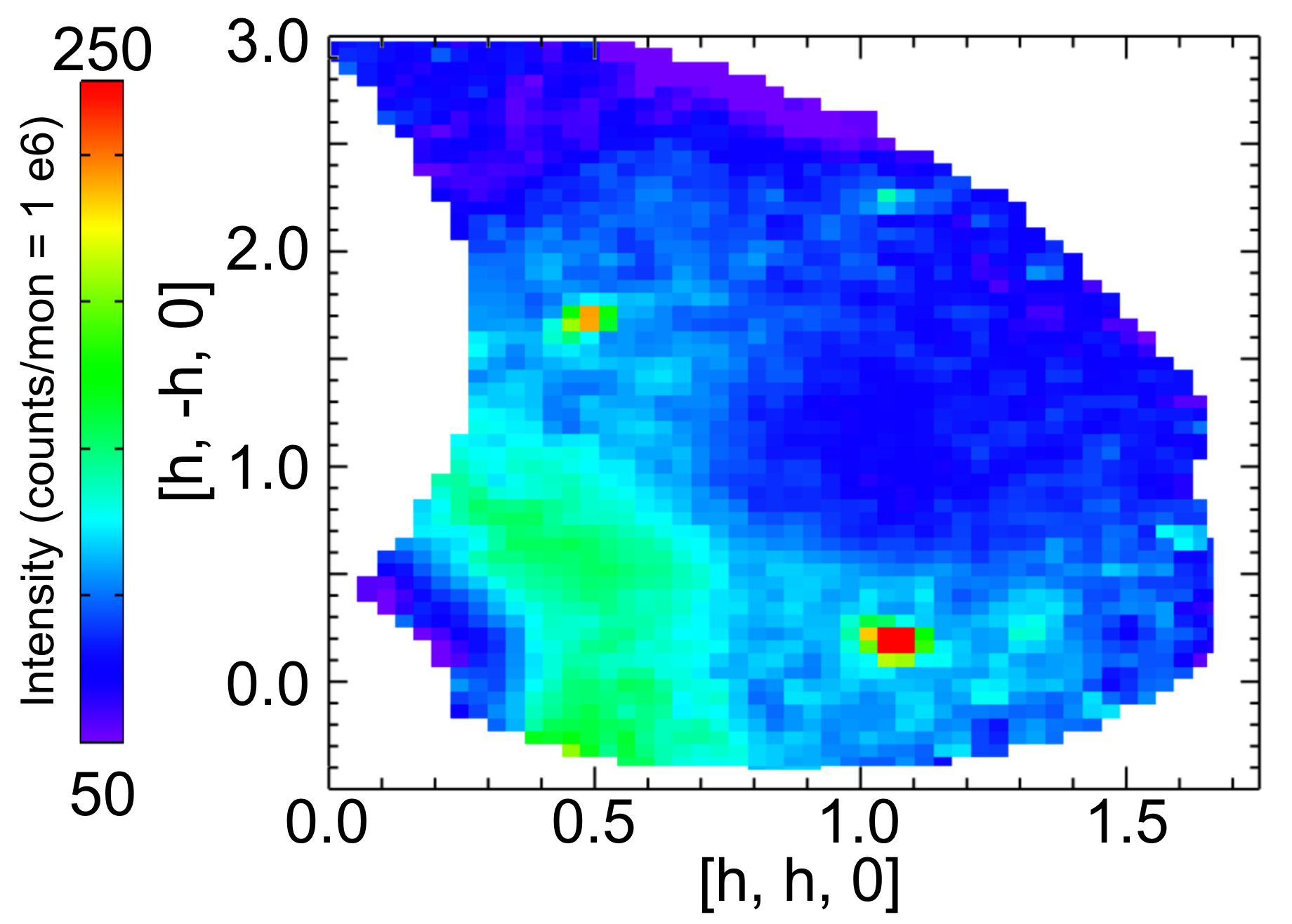
(c) (c) $E=$ 0.65 meV

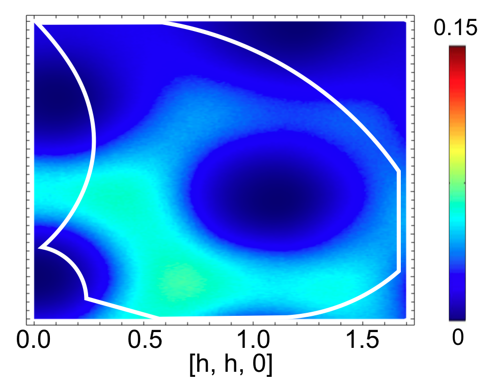
(d) (d) $E=$ 0.46 meV

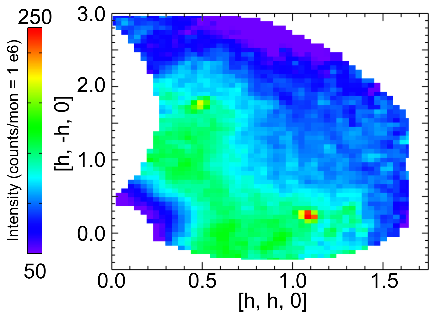
(e) (e) $E=$ 0.9 meV

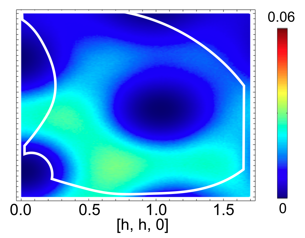
(f) (f) $E=$ 1.15 meV

Figure 2: Fluctuations in the spin-liquid phase of Ca₁₀Cr₇O₂₈, showing ${\bf q}$–dependent structure on different energy scales. (a) INS data for Ca₁₀Cr₇O₂₈ at low energy, suggestive of a “ring” of scattering, centered on $(2,0,0)$. (b) Equivalent results from molecular dynamics (MD) simulations. (c) INS data for Ca₁₀Cr₇O₂₈ at intermediate energy, showing “bow-tie” structures centered on $(1,0,0)$. (d) Equivalent results from MD simulation. (e) Cut through inelastic neutron scattering (INS) data for Ca₁₀Cr₇O₂₈ at high energy, also showing “bow-tie” structure. (f) Equivalent results from MD simulation. Experimental data are reproduced from Balz et al. (2016), with measurements carried out at $T=90\ \text{mK}$. MD simulations were carried out for a bilayer breathing Kagome (BBK) model, at $T=220\ \text{mK}$, as described in the text. Energies were chosen so as to compare corresponding features in simulation and experiment.

We also study the evolution of the dynamical and thermodynamical properties of the BBK model in applied magnetic field, concentrating on parameters relevant to Ca₁₀Cr₇O₂₈ [Fig. 3].

We find that the onset of the spin–liquid observed in experiment is associated with the closing of a gap to transverse spin excitations, at a field $B^{*}(T)$, with $B^{*}(220\ \text{mK})\approx 0.7\ \text{T}$, and $B^{*}(T\to 0)\to 1.1\ \text{T}$. From the nature of the spin excitations when this gap closes, we identify the low–field state as a gapless, “spiral spin–liquid”, known for ring–like correlations in $S({\bf q})$ Bergman et al. (2007); Okumura et al. (2010); Benton and Shannon (2015); Seabra et al. (2016); Buessen et al. (2018); Yao et al. (2021). Simulations also reveal low–energy, longitudinal excitations, which may explain the anomalously high specific heat measured at low temperatures. At the lowest temperatures, we find a complex set of competing orders including the finite–field extension of the lattice nematic and a multiple–q state. Finally, we show how the field–saturated state provides an opportunity to study the “half–moons” recently discussed in the context of Kagome antiferromagnets Yan et al. (2018); Mizoguchi et al. (2018). Taken together, these results provide a broad characterisation of the BBK model of Ca₁₀Cr₇O₂₈, within a (semi–)classical approximation which explains many of the features seen in experiment.

The remainder of this Article is structured as follows:

In Sec. II we review the existing experimental and theoretical literature on Ca₁₀Cr₇O₂₈, and introduce the spin–1/2 bilayer breathing–Kagome (BBK) model used to interpret these results.

In Sec. III we present simulation results for the thermodynamics of the BBK model of Ca₁₀Cr₇O₂₈ in zero magnetic field. Classical Monte Carlo (MC) results are used to construct a finite–temperature phase diagram which connects the spin liquid phase of Ca₁₀Cr₇O₂₈ with a domain of high classical ground–state degeneracy of the BBK model.

In Sec. IV we show corresponding results for dynamics, taken by numerically integrating the equations of motion for states drawn from MC simulation (MD simulation). Results are visualised through both animations and plots of the dynamical structure factor $S({\bf q},\omega)$, which are used to connect with experiment.

In Sec. V we turn to the thermodynamic properties of the BBK model in applied magnetic field. Classical MC simulation is used to establish a phase diagram as a function of field and temperature, for parameters appropriate to Ca₁₀Cr₇O₂₈.

In Sec. VI we explore the corresponding changes in spin dynamics as function of magnetic field, again through numerical integration of equations of motion (MD simulation). Particular attention is paid to the way in which the spin liquid emerges from the paramagnet found at high values of magnetic field.

In Sec. VII we discuss the implication of these results for the understanding of Ca₁₀Cr₇O₂₈.

Finally, in Sec. VIII we conclude with a brief summary of results and open questions.

Further technical information is provided in a short series of Appendices:

Appendix A contains technical details of the classical Monte Carlo (MC) and Molecular Dynamics (MD) techniques used in this study, as well as of the methods used to animate spin configurations.

Appendix B contains technical details of the Animation of spin configurations.

Appendix C contains details of the structure factors and form factors used when comparing with experiment.

Appendix D provides details of an estimate of the Wilson ratio for Ca₁₀Cr₇O₂₈.

(a)

Figure 3: Schematic phase diagram of the classical bilayer breathing Kagome (BBK) model of Ca₁₀Cr₇O₂₈, as function of temperature and magnetic field. At high temperatures individual spin–1/2 moments fluctuate independently. For $T\approx 500\ \text{mK}$ there is a crossover into a regime in which spins on triangular plaquettes form effective spin–3/2 moments. For fields $B\lesssim 1\ \text{T}$ these form a spiral spin liquid, characterised by a ring–like structure in the dynamical structure factor $S({\bf q})$. At temperatures $T\lesssim 60\ \text{mK}$, this gives way to states which break discrete symmetries of the lattice, including a lattice nematic, and a multiple–q state. This hierarchy of temperature and field scales is derived from classical Monte Carlo (MC) simulations described in Section III and in Section V. The temperature for which dynamics have been characterised in detail, $T=220\ \text{mK}$, is shown with a white dashed line [cf. Fig. 2].

II $\text{Ca}_{10}\text{Cr}_{7}\text{O}_{28}$ and the BBK model

While the study of Ca₁₀Cr₇O₂₈ has a short history, a wide range of different experimental and theoretical techniques have already been brought to bear on it. In what follows we review attempts to unravel the properties of Ca₁₀Cr₇O₂₈, starting from its chemistry and structure, and covering different aspects of its experimental characterisation, before surveying attempts to model it in terms of a bilayer breathing–Kagome (BBK) model. A brief account is also given of the closely–related physics of the $J_{1}$–$J_{2}$ Heisenberg model on a honeycomb lattice.

II.1 Chemistry and crystal structure

The earliest motivation for studying Ca₁₀Cr₇O₂₈ came from chemistry. In oxides, Cr is typically found with a $3+$ valence, giving rise to magnets with spin–3/2 moments. A typical example of such is the spinel CdCr₂O₄, a relatively classical magnet, interesting for the interplay between magnetic frustration and spin–lattice coupling — see e.g. Rossi et al. (2019). Ca₁₀Cr₇O₂₈, on the other hand, is one of a family of materials exhibiting the unusual, spin–1/2, Cr⁵⁺ valence state Gyepesová and Langer (2013); Arcon et al. (1998). And the spin–1/2 nature of the magnetic ions in Ca₁₀Cr₇O₂₈ brings with it physics of an altogether more quantum nature than is found in CdCr₂O₄.

Structurally, Ca₁₀Cr₇O₂₈ has much in common with SrCr₂O₈, a Mott insulator based on Cr⁵⁺ ions, which has been studied for its quantum dimer ground state Wang et al. (2016). SrCr₂O₈ is composed of stacked, triangular–lattice bilayers, and has the high–temperature space group R3$\overline{m}$, Cuno and Müller-Buschbaum (1989). At $T=275\ \text{K}$, it undergoes a structural phase transition into a phase with space group C2/c, lifting the orbital degeneracy of the Cr⁵⁺ ions Islam et al. (2010). This promotes a low–temperature phase in which Cr⁵⁺ form a triangular lattice of singlet dimers, each arranged along the c-axis connecting the two planes of each bilayer Islam et al. (2010); Quintero-Castro et al. (2010); Wang et al. (2016).

Ca₁₀Cr₇O₂₈ differs from SrCr₂O₈ through the inclusion of non–magnetic Cr⁶⁺ ions, at a ratio of 6 Cr⁵⁺ ions to 1 Cr⁶⁺ Arcon et al. (1998). These convert the stacked, triangular bilayers of SrCr₂O₈ into weakly–coupled bilayers of a “breathing” kagome lattice, in which triangular plaquettes have alternating size Balz et al. (2017b); Balodhi and Singh (2017) — cf. Fig. 1. This bilayer breathing–Kagome (henceforth, BBK) lattice has a very low symmetry, with the space group identified as R3c Gyepesová and Langer (2013); Balz et al. (2017b). Within this space group, the magnetic Cr⁵⁺ ions have a 6–site unit cell, and the Cr⁵⁺ site is located within a (distorted) CrO₄ tetrahedron. The crystal field at this site is sufficiently low that the degeneracy of the $e_{g}$ orbitals is quenched, leaving a single 3d electron in a single orbital, i.e. a spin–1/2 moment.

	$\gamma$	$\chi_{0}$	$\mu_{\sf eff}$	$R_{\sf W}$
	[mJ mol-1 K-2]	[emu mol-1 Oe-1]	[$\mu_{B}$]
Cu	$0.695$	weakly diagmagnetic	1.7	n/a
CeCu6 Ott (1987); Amato et al. (1987)	$1550$	$0.3$	2.5	$4$
Ca10Cr7O28  Sonnenschein et al. (2019); Kshetrimayum et al. (2020)	$13500$	$3.0$	1.7	16.2

Table 1: Comparison of the low temperature thermodynamic properties of Ca₁₀Cr₇O₂₈ with the conventional metal Cu, and the heavy fermion material CeCu₆. The parameters shown are the linear coefficient of specific heat $C(T\to 0)=\gamma T$; the paramagnetic susceptibility $\chi(T\to 0)=\chi_{0}$, effective moment $\mu_{\sf eff}$, and the Wilson ratio $R_{W}$ [Eq. (42)].

II.2 Thermodynamic properties

The thermodynamic properties of Ca₁₀Cr₇O₂₈ distinguish it as a frustrated magnet in which spins interact, but continue to fluctuate down to very low temperatures. The magnetic susceptibility of Ca₁₀Cr₇O₂₈ displays a Curie–law behaviour

$$\chi^{-1}(T)\approx\frac{T-\theta_{\sf CW}}{C}$$ (2)

down to temperatures of a few Kelvin. A positive Curie–Weiss temperature of

$$\theta_{\sf CW}=2.35\ \text{K}\;,$$ (3)

consistent with dominant FM interactions, was reported by Balz et al. Balz et al. (2016, 2017a), with the slightly higher value of $\theta_{\sf CW}=4.1(6)\ \text{K}$ being reported by Balodhi and Singh Balodhi and Singh (2017). Both groups find a value of $C$ consistent with an effective moment

$$\mu_{\sf eff}\approx 1.7\ \mu_{B}$$ (4)

at each Cr⁵⁺ site, as would be expected for a spin–1/2 moment, assuming a Landé factor $g=2$.

At low temperatures, the magnetisation of Ca₁₀Cr₇O₂₈ rises rapidly in applied magnetic field, consistent with a gapless ground state Balz et al. (2017a); Kshetrimayum et al. (2020). At low fields, the magnetisation is found to be nearly linear in $B$, with an associated susceptibility

$$\chi_{0}=3.0\ \text{emu/mol\ Oe}\;,$$

at $T=1.8\ \text{K}$; a large value even by comparison with heavy Fermion materials [Table 1]. This behaviour stands in marked contrast with SrCr₂O₈, where the energy gap from the dimerized ground–state to the lowest–lying triplet excitation ensures that the magnetisation remains zero up to a field $H_{c1}=30.4\ \text{T}$ Quintero-Castro et al. (2010); Wang et al. (2016). The magnetization of Ca₁₀Cr₇O₂₈ is also broadly independent of the direction in which field is applied, and saturates at a relatively low field, with a sharp kink in $M(H)$ observed at a scale of $H\sim 1\ \text{T}$, and complete saturation is observed for fields no greater than $H\sim 10\ \text{T}$, at a temperature of $1.8\ \text{K}$ Balz et al. (2016, 2017a).

Heat capacity measurements carried out in zero field by Balz et al. Balz et al. (2016, 2017a) offer a consistent picture, with a dramatic kink in $C(T)$ at $T\approx 500\ \text{mK}$, a broad maximum at $T\approx 3.1\ \text{K}$, and no evidence for either magnetic order, or the opening of a spin–gap, down to $T=300\ \text{mK}$. The measured values of $C(T)$ at this temperature are consistent with a high density of low–lying excitations, with $C/T$ achieving values $\sim 14\ \text{J\ mol${}^{-1}$\ K${}^{-2}$}$ Balz et al. (2017a) which, again, are large even by the standard of heavy–fermion materials [Table 1]. Later experiments, reported by Sonnenschein et al. Sonnenschein et al. (2019), extended measurements down to $T=37\ \text{mK}$, finding a nearly linear specific heat $C(T)\approx\gamma T$ over the temperature range $100\ \text{mK}\lesssim T\lesssim 500\ \text{mK}$, with

$$\gamma=13.5\ \text{J\ mol${}^{-1}$\ K${}^{-2}$}\;.$$

For $37\ \text{mK}<T\lesssim 100\ \text{mK}$, measurements find $C(T)<\gamma T$, showing a slight suppression relative to a purely linear behaviour, but no evidence for a gap to excitations. Meanwhile, at higher $T$, in the absence of magnetic field, $C/T$ is a monotonically–decreasing function of temperature Balz et al. (2017a). Qualitatively similar results for $C(T)$ at higher temperatures were also reported by Balodhi and Singh Balodhi and Singh (2017), with the caveat that the measured values differ by a numerical factor $\sim 2$ between the two groups.

In applied magnetic field, the values of $C/T$ found at low temperatures steadily decrease, and plots of $C/T$ acquire a shoulder at $T\lesssim 1\ \text{K}$ Balz et al. (2017a). A qualitative change occurs for $B\approx 1\ \text{T}$, when a downturn become visible in $C/T$ at low temperatures, consistent with suppression of low–lying excitations by the opening of a gap. Attempts to model the field–temperature dependence of $C(T)$ as the sum of $T^{3}$ contribution from phonons, and Shottky anomaly (broad peak) coming from spin excitations, meet with some success. However this approach fails to explain the relatively high density of low–lying excitations seen in experiment, especially if the Shottky peak is associated with the gap measured in inelastic neutron scattering, as described below Balz et al. (2017a).

II.3 Macroscopic dynamics

Meanwhile, measurements of AC susceptibility $\chi(\nu,T)$, for frequencies $\nu\lesssim 20\ \text{kHz}$, exhibit a broad peak at a temperature $T^{*}\sim 330\ \text{mK}$ Balz et al. (2016). Under other circumstances, this might hint at spin–glass freezing. However Cole–Cole plots of the real against imaginary parts of $\chi$ remain semi–circular for temperatures both above and below $T^{*}$, suggesting that a single timescale governs the macroscopic relaxational dynamics of Ca₁₀Cr₇O₂₈, even at low temperatures Balz et al. (2016). Consistent with this, $\mu$SR measurements reveal persistent spin fluctuations down to $19\ \text{mK}$, with the measured relaxation rates increasing with decreasing temperature, and saturating for $T<T^{*}$ Balz et al. (2016).

The picture painted by these experiments is one of a magnet whose moments continue to fluctuate down to temperatures two orders of magnitude smaller than the characteristic scale of exchange interactions. A clear hierarchy of other temperature and field scales emerges, with both $\theta_{\sf CW}$, and the broad maximum in $C(T)$, picking out a scale of $T\approx 3\ \text{K}$; AC susceptibility and $\mu$SR revealing changes in dynamics at $T\approx 330\ \text{mK}$; and magnetisation and heat capacity suggesting a change of phase at $B\approx 1\ \text{T}$. This behaviour would be hard to reconcile with any simple paramagnet, and is entirely consistent with a quantum spin liquid. But from these measurements alone, it is difficult to confirm the collective nature of spin fluctuations, or to say what kind of spin liquid might be found in Ca₁₀Cr₇O₂₈.

II.4 Neutron scattering

More insight into the nature of magnetic correlations in Ca₁₀Cr₇O₂₈ can be gained through the structure factor measured in neutron scattering. Neutron scattering has been carried out on both powder and single–crystal samples of Ca₁₀Cr₇O₂₈, using a variety of different neutron instruments Balz et al. (2016, 2017a); Sonnenschein et al. (2019). Elastic scattering fails to reveal any magnetic Bragg peaks down to $90\ \text{mK}$, consistent with the absence of any other signals of long–range magnetic order. At the lowest energies experiments reveal instead a quasi–elastic signal, extending up to $\sim 0.2\ \text{meV}$. This quasi–elastic signal is essentially independent of ${\bf q}$, on the scale of the BZ, and has been attributed to incoherent scattering from randomly distributed nuclear isotopes Balz et al. (2016). Magnetic scattering is inelastic in character, and highly structured, confirming the collective nature of spin fluctuations. Strong scattering for $\omega\lesssim 0.4\ \text{meV}$ echoes the characteristic temperature scale seen in thermodynamic measurements. However this is clearly not the only energy scale in the problem; a further strong signal is seen at $\omega\sim 1\ \text{meV}$, accompanied by a broad background of scattering extending up to $\omega\sim 1.5\ \text{meV}$. Consistent with the lack of magnetic Bragg peaks, no hint is found of the spin waves which would be associated with the breaking of spin–rotation symmetry.

The strong ${\bf q}$– and $\omega$–dependence of scattering is evident in energy cuts through the measured dynamical structure factor $S({\bf q},\omega)$, reproduced in Fig. 2. Scattering at low energies provides the most information about correlations in the ground state, but unfortunately is obscured by the incoherent signal for $\omega\lesssim 0.2\ \text{meV}$. None the less, measurements at $0.25\ \text{meV}$ [Fig. 2a] reveal that low–energy fluctuations are strongly ${\bf q}$–dependent, with hints of a ring–like structure centered on $(2,0,0)$. (Much stronger scattering seen at other zone centers reflects phonons Balz et al. (2016)). The scattering at an intermediate energy of $0.65\ \text{meV}$ [Fig. 2c] is also strongly ${\bf q}$–dependent, but reveals a completely different kind of correlation. In this case, instead of a “ring” at $(2,0,0)$, experiments suggest a “bow-tie” centered on $(1,0,0)$. And the same bow–tie pattern is more clearly visible at the relatively high energy of $0.9\ \text{meV}$ [Fig. 2e].

It is worth noting, that energy values in MD simulations have been slightly shifted, to allow for a qualitative comparison of the scattering pattern to INS experiments. While the main features, namely “rings” at low energy and “bow-ties” at higher energy, could be reproduced well within our (semi-)classical method, they occur at slightly different energies. This renormalisation is presumably due in the approximations inherent in both the BBK model of Ca₁₀Cr₇O₂₈ (which neglects anisotropic exchange interactions), and our (semi–)classical treatment of its dynamics. We will revisit this last point in a coming work Shimokawa et al. (tion).

II.5 The BBK model

Taken together, both thermodynamic and dynamical measurements of Ca₁₀Cr₇O₂₈ are consistent with the existence of a gapless (or nearly gapless) quantum spin liquid at low temperatures. This phenomenology contains elements which are familiar from the behaviour of other magnets, such as the bow–tie patterns observed in scattering at higher energies, reminiscent of the pinch–points observed in Coulombic phases Henley (2010). However, while there are plenty of examples of studies of two–dimensional quantum spin liquids Balents (2010); Savary and Balents (2016); Anderson (1973); Lee (2008); Shimizu et al. (2003); Knolle and Moessner (2019); Zhou et al. (2017); Masutomi et al. (2004); Han et al. (2012); Kitaev (2006); Jackeli and Khaliullin (2009); Banerjee et al. (2016); Baek et al. (2017); Winter et al. (2017); Hermanns et al. (2018), no model or material provides a complete analogue to the behaviour of Ca₁₀Cr₇O₂₈, even at a qualitative level. And the fact that Ca₁₀Cr₇O₂₈ displays such different behaviour on different energy scales means that a low–energy effective theory alone cannot unlock all of its secrets. To make further progress in understanding Ca₁₀Cr₇O₂₈, a microscopic model is therefore needed.

The simplest model one can consider for Ca₁₀Cr₇O₂₈ is one in which both orbital effects, and spin–orbit coupling, are neglected, so that each Cr⁵⁺ ion is treated as a spin–1/2 moment, interacting through Heisenberg interactions. The neglection of other terms allowed by lattice symmetry, such as Dzyaloshinskii–Moriya (DM) interactions, finds some justification in the 3d nature of the magnetic electrons, and the lack of magnetic anisotropy observed in experiment. However even a minimal, $SU(2)$–symmetric model, will have many different parameters, since the BBK lattice supports seven inequivalent first–neighbour bonds Balz et al. (2016, 2017a). And ultimately, the extent to which one can parameterise such a complex model from experiment, and use it to understand the novel physics of Ca₁₀Cr₇O₂₈, becomes an empirical question.

Fortunately, the low saturation field of Ca₁₀Cr₇O₂₈ means that it is possible to parameterise a minimal, microscopic model for its magnetism from inelastic neutron scattering (INS) experiments on its field–polarised state. These reveal gapped, two–dimensional spin–wave excitations (discussed in Section VI.1, below) which, within experimental resolution, are adequately described by a Heisenberg model for a single bilayer Balz et al. (2016, 2017a),

$${\cal H}_{\sf BBK}=\sum_{\langle ij\rangle}J_{ij}{\bf S}_{i}\cdot{\bf S}_{j}-B\sum_{i}S^{z}_{i}\;,$$ (5)

introduced as Eq. (1). This spin–1/2 BBK model has 5 first–neighbour couplings within a single bilayer [Fig. 1], of which 3 are ferromagnetic (FM) and 2 antiferromagnetic (AF) [Table 2]. The strongest interactions, $J_{21}\approx-0.8\ \text{meV}$ and $J_{22}\approx-0.3\ \text{meV}$, are FM and occur within the triangular plaquettes of the BBK lattice. Meanwhile, the couplings between these plaquettes are FM in the interplane direction, $J_{0}\approx-0.1\ \text{meV}$, and AF within the breathing–Kagome planes; $J_{31},J_{32}\approx 0.1\ \text{meV}$.

The picture of Ca₁₀Cr₇O₂₈ which emerges is therefore one of strongly–coupled FM plaquettes, which are in turn coupled AF within a single breathing–Kagome plane, and FM between the two layers.

${\cal H}_{\text{\sf BBK}}$ [Eq. (1)]	Ca10Cr7O28 Balz et al. (2016, 2017a)	${\cal H}_{\text{\sf HC}}$ [Eq. (6)]
$J_{\text{0}}$	$-0.08(4)\ \text{meV}$	$J_{\text{1}}$
$J_{\text{21}}$	$-0.76(5)\ \text{meV}$	–
$J_{\text{22}}$	$-0.27(3)\ \text{meV}$	–
$J_{\text{31}}$	$\phantom{-}0.09(2)\ \text{meV}$	$J_{\text{2}}$
$J_{\text{32}}$	$\phantom{-}0.11(3)\ \text{meV}$	$J_{\text{2}}$

Table 2: Exchange interactions within the bilayer breathing–Kagome (BBK) model of Ca₁₀Cr₇O₂₈, [Eq. (1)], as estimated from inelastic neutron scattering in high magnetic field Balz et al. (2016, 2017a). Bond indices $J_{ij}$, following the conventions of Balz et al. Balz et al. (2016, 2017a), are defined in Fig. 1. Also listed are the corresponding interactions within an effective spin–3/2 honeycomb–lattice model [Eq. (6)], with bond indices defined in Fig. 4.

II.6 Theoretical work based on the BBK model

While even this, minimal model of Ca₁₀Cr₇O₂₈ may seem alarmingly complicated, it does provide a concrete microscopic starting point for understanding experiment, and here some good progress has already been made.

A straightforward, but informative exercise, is to use linear spin wave (LSW) theory to track the evolution of $S({\bf q},\omega)$ with magnetic field Balz et al. (2017a). Mean–field theory for Eq. (1), using experimental parameters [cf. Table 2], predicts that the saturated state is stable for $B>1.1\ \text{T}$. Meanwhile LSW for Eq. (1) gives a qualitatively reasonable description of the scattering observed in experiment, and its field evolution for $B\gtrsim 1\ \text{T}$ Balz et al. (2017a).

More sophisticated methods have been applied to the spin–liquid ground state found for $T=0$. Pseudofermion functional renormalisation group (PFFRG) calculations for the BBK model Eq. (1) Balz et al. (2016), find a disordered ground state for a range of parameters centered on those found in experiment. And, encouragingly, PFFRG calculations of the static structure factor, $S({\bf q},\omega=0)$, exhibit a ring–like structure, similar to that observed in experiment. The stability of this spin liquid state is, interestingly, found to depend on the differences in parameters between the different planes of the bilayer, with symmetric choices leading to ordered ground states.

Subsequent tensor–network calculations, based on “projected entangled simplex states” (PESS) Kshetrimayum et al. (2020), also predict a spin–liquid ground state. This approach has been used to estimate the ground–state magnetisation for parameters taken from Ca₁₀Cr₇O₂₈ [cf. Table 2]. At low fields, the magnetisation is found to be nearly linear in $B$, with associated susceptibility

$$\chi_{\sf PESS}=1.1731\ \text{$\mu_{B}$/Cr${}^{5+}$ T}=3.93\ \text{emu/mol\ Oe}\;,$$

about 30 % larger than the value observed in experiments carried out at $T=1.8\ \text{K}$ Balz et al. (2017a). The same calculations find a saturation field of $B\approx 1\ \text{T}$ Kshetrimayum et al. (2020).

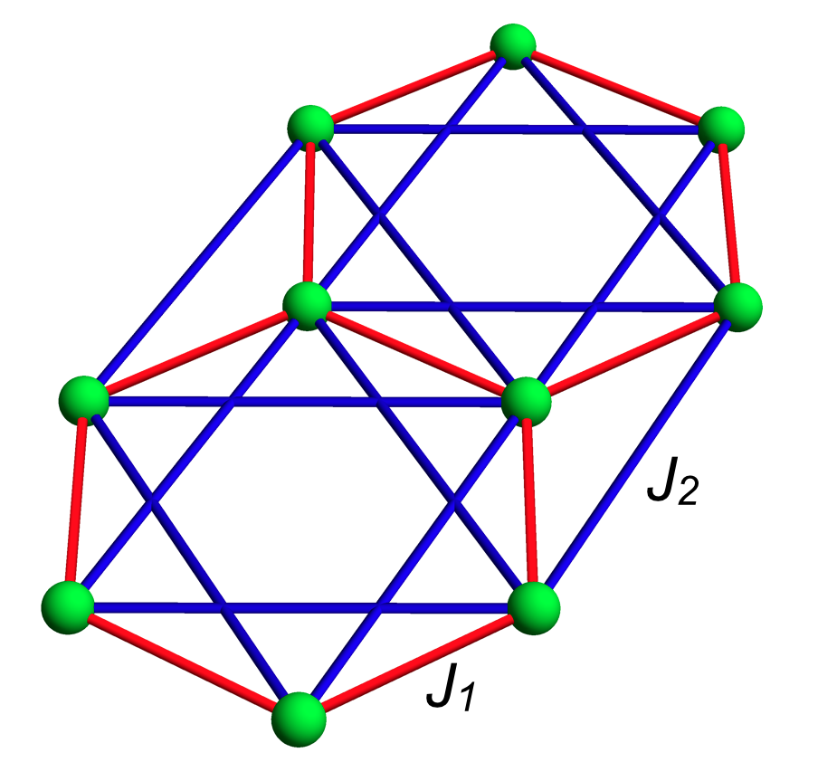
Figure 4: Honeycomb lattice realised by triangular plaquettes of spins in Ca₁₀Cr₇O₂₈, cf. Fig. 1. Labelling of bonds identifies parameters of the effective spin–3/2 model, Eq. (6). Experimental estimates of these parameters can be found in Table 2.

A phenomenological approach to the low–temperature properties of Ca₁₀Cr₇O₂₈ has also been developed by Sonnenschein et al. Sonnenschein et al. (2019). Taking inspiration from the broad continuum found in inelastic neutron scattering Balz et al. (2016), and the (nearly) linear specific heat at low temperatures, these authors introduce a model of non–interacting Fermionic spinons hopping on a (decorated) honeycomb lattice. This model is not derived directly from Eq. (1), but respects the symmetries of the BBK lattice, and is parameterised so as to reproduce the energy scales and some of the key qualitative features of the scattering seen in experiment. It has three two–fold degenerate bands; the lower occupied band has a nearly circular hole–like Fermi surface, while the unfilled high–energy bands mirror the dispersion of graphene. This approach which corresponds to a $U(1)$ QSL, reproduces the rings of scattering in $S({\bf q},\omega)$ at low energy $\hbar\omega\sim 0.15\ \text{meV}$, and suggests features at intermediate energy $\hbar\omega\sim 0.85\ \text{meV}$ which contain at least relics of pinch–point structure.

By introducing further phenomenological parameters for pairing of spinons, Sonnenschein et al. are also able to model the deviation from $T$–linear specific heat found for $35\ \text{mK}<T<100\ \text{mK}$ Sonnenschein et al. (2019). The best fits are found for an f–wave gap, leading to a Fermi surface with Dirac points, and implying a $\mathbb{Z}_{2}$ spin liquid ground state Senthil and Fisher (2000). This spinon pairing also “cures” a seeming contradiction with experiment, since a $U(1)$ QSL would show additional, divergent, contributions to $C(T)$ coming from gapless gauge fluctuations Senthil et al. (2004); Motrunich (2005).

II.7 Effective honeycomb lattice model

Phenomenology aside, published theory for quantum effects in Ca₁₀Cr₇O₂₈ are limited to its ground state. Also, very little is known about the properties of the spin–1/2 BBK model at finite temperature. Some progress has however been made in the classical limit, by considering a simplified, spin–3/2 model.

The strongest couplings in the BBK model of Ca₁₀Cr₇O₂₈ are the FM interactions within the triangular plaquettes of the BBK lattice, $J_{\text{21}}\approx-0.76\ \text{meV}$ and $J_{\text{22}}\approx-0.27\ \text{meV}$ (cf. shaded green triangles in Fig. 1). This immediately suggests a simplification, namely treating each plaquette as a spin–3/2 moment on the medial, honeycomb lattice

$${\cal H}_{\hexagon}=J_{1}\sum_{\langle ij\rangle_{1}}\ {\bf S}_{i}\cdot{\bf S}_{j}+J_{2}\sum_{\langle ij\rangle_{2}}{\bf S}_{i}\cdot{\bf S}_{j}-B^{z}\sum_{i}S^{z}_{i}\;,$$ (6)

where the first–neighbour coupling $J_{1}\approx-0.08\ \text{meV}$ corresponds to the FM inter–layer coupling $J_{\text{0}}$ in the original BBK model, while the second–neighbour coupling $J_{2}\approx 0.10\ \text{meV}$ can be taken to be the mean of the AF intra–layer interactions $J_{\sf eff}$ as

$$J_{\sf eff}\equiv(J_{31}+J_{32})/2\;.$$ (7)

Classically at least, this simplified model can be expected to give a reasonable account for the properties of Ca₁₀Cr₇O₂₈ for $T,\omega<J_{\text{21}},J_{\text{22}}$.

Working with a spin–3/2 model on a honeycomb lattice has the added advantage that it connects Ca₁₀Cr₇O₂₈ with an established literature on unconventional magnetic phases in honeycomb–lattice models with competing interactions Rastelli et al. (1979); Fouet et al. (2001); Mulder et al. (2010); Okumura et al. (2010). The $J_{1}$–$J_{2}$ Heisenberg model Eq. (6), is a special case of the $J_{1}$–$J_{2}$–$J_{3}$ Heisenberg model on honeycomb lattice, where third–neighbour interactions are also taken into account. The classical ground states of this parent model are distinguished by the competition between the different forms of coplanar spiral order. And, for $J_{3}=0$, where spirals with different ordering wave vectors meet, a continuous manifold of ground states is formed, with wave vectors belonging to a ring–like locus of points in $\mathbf{q}$–space [Fig. 5].

Depending on parameters, this ring can be centered on the $\Gamma$ point at the center of the Brilluoin zone (BZ) Rastelli et al. (1979); Fouet et al. (2001); Okumura et al. (2010), or on the K–point at the corner of the BZ Mulder et al. (2010). Both of these cases have already been studied for AF $J_{1}$. In the case of the “large” ring centered on $\Gamma$, spin liquids with “ring” or “pancake” motifs are found at high temperatures, while at very low temperatures, a phase transition is identified into a state breaking the 3–fold rotation symmetry of the lattice Okumura et al. (2010). Very similar results are found for the “small” ring centered on $K$, where the transition into the ordered phase was identified as a 3–state Potts transition Mulder et al. (2010).

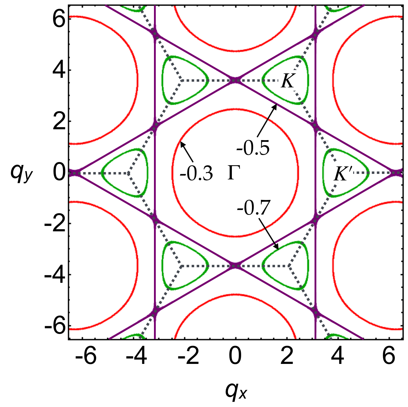
Figure 5: Loci of degenerate classical ground states in the $J_{1}$–$J_{2}$ Heisenberg model on a honeycomb lattice, Eq. (6). Depending on the ratio of parameters, these loci may take the form of “large” rings centered on $\Gamma$ Rastelli et al. (1979); Fouet et al. (2001); Okumura et al. (2010), or “small” rings centered on $K$ Mulder et al. (2010); Biswas and Damle (2018). Here, results are shown for $J_{2}/J_{1}=-0.3$ (red line), $-0.5$ (purple) and $-0.7$ (green).

Biswas and Damle have extended the analysis of Eq. (6) to the case of FM interactions $J_{1}<0$, through a combination of classical MC simulation, MD simulation, spin–wave theory, and large–N calculations Biswas and Damle (2018). Considering the limit $B=0$, a ratio of parameters $J_{1}/J_{2}$ motivated by Ca₁₀Cr₇O₂₈ [cf. Table 2], they find that fluctuations select a discrete set of spiral states from the “small” ring of ground states centered on ${\bf q}=K$. Corresponding MC simulations of Eq. (6) reveal a 3–state Potts transition into a state breaking lattice rotation symmetry at $T^{*}\approx 66\ \text{mK}$, consistent with Mulder et al. (2010). This is accompanied by critical slowing down in the dynamics found in MD simulation, and a large but finite spiral-correlation length. Close to $T^{*}$, the equal–time structure factor $S({\bf q})$ shows a locus of highly–degenerate states near the K-points of the Brillouin zone, consistent with the “small” ring. At higher temperatures, $S({\bf q})$ instead shows a larger ring of scattering, near the zone boundary, similar to that observed in Ca₁₀Cr₇O₂₈ Balz et al. (2016).

Quantum effects within the $J_{1}$–$J_{2}$ honeycomb lattice model have only been studied in detail for $S=1/2$. In this case the phase breaking lattice rotation symmetry is proposed to be a valence bond solid (VBS) Mulder et al. (2010), and QSL states have been proposed elsewhere for both FM Fouet et al. (2001) and AF $J_{1}$ Fouet et al. (2001). In the case of $S=3/2$, spin–wave estimates suggest that spiral order is unstable for parameters relevant to Ca₁₀Cr₇O₂₈ Biswas and Damle (2018), but do not reveal the nature of any competing QSL.

Figure 6: (a) Finite–temperature phase diagram of the BBK model, Eq. (1), showing wide extent of spin liquid phase. Result are shown as a function of $x=J_{\sf eff}/J_{0}$ [Eq. (7)], and all other parameters taken from experiment [Table 2]. The temperatures at which inelastic neutron scattering (INS) experiments were carried out on Ca₁₀Cr₇O₂₈ are shown with white dots, at $x=-1.25$ Balz et al. (2016, 2017a). (b) Classical ground–state phase diagram of the corresponding honeycomb-lattice model, Eq. (6), as a function of $x=J_{2}/J_{1}$, following [Rastelli et al., 1979; Fouet et al., 2001; Mulder et al., 2010]. (c) Equal–time structure factor $S({\bf q})$ at for $x=-1.25$, $T=220\ \text{mK}$; the boundary of the Brillouin Zone (BZ) is shown with white lines. Strong correlations are observed near the boundary of the $1^{st}$ BZ, with the highest intensity centered on the K–points at zone corners. Form factors associated with magnetic correlations have the periodicity of the $4^{th}$ BZ, shown here with red lines. (d) Equivalent results at $x=-1.25$, $T=90\ \text{mK}$, showing how scattering from the “small” ring centered on K-points becomes sharper at low temperatures. All results were obtained from classical Monte Carlo (MC) simulation of Eq. (1), as described in Sec. III and Appendix A, for a cluster of linear dimension L = 48 (N = 13,824). Phase boundaries in (a) were determined from the sharp peak in specific heat $C(T)$ associated with either the breaking of lattice–rotation symmetry, or the onset of ferromagnetic (FM) fluctuations.

II.8 Open questions

While considerable progress has been made, the complex phenomenology of Ca₁₀Cr₇O₂₈ has yet to find any complete, or microscopically–grounded explanation. On the experimental side, further tests of spin liquid properties through, e.g. thermal transport, could bring new insights. And improvements in the resolution of inelastic scattering would also be very valuable, making it possible to better–constrain microscopic or phenomenological models, and to more accurately test proposals about the spin–liquid state.

Meanwhile, obvious challenges for theory include:

1. connecting the finite–energy and finite–temperature properties of Ca₁₀Cr₇O₂₈ with the spin–1/2 BBK model, Eq. (1);

2. extending the analysis of this model to finite magnetic field ;

3. identifying the mechanism driving its low–temperature spin liquid state;

4. identifying interesting properties of the BBK model which may, as yet, be obscure in experimental data for Ca₁₀Cr₇O₂₈.

In this Article, and the one which follows Shimokawa et al. (tion), we continue the project, begun in Pohle et al. (2017), of addressing the points (i)–(iv) above. The results in this first Article are drawn exclusively from (semi–)classical methods: Monte Carlo simulation; linear spin-wave theory; and numerical intergration of equations of motion for spins, which we refer to as molecular dynamics (MD) simulation. And before embarking on this journey, some comment is due on the validity of using classical methods to address questions such as these, in a quantum magnet.

Ca₁₀Cr₇O₂₈ is a highly–frustrated, quasi–two dimensional system, with spin–1/2 moments, and a strong candidate for a quantum spin liquid (QSL) Balz et al. (2016). So it might at first seem that there was little to be learnt from classical techniques. None the less, experience with other models that support QSL, where exact (or numerically exact) quantum results are available for comparison — notably the Kitaev model Samarakoon et al. (2017), and quantum spin ice Taillefumier et al. (2017); Benton et al. (2018)) — teaches that, suitably interpreted, classical approaches yield a surprising amount of insight into both the correlations and dynamics of quantum spin liquids at finite temperature. Moreover, classical simulations always bring meaningful advantage in terms of the size of the system that can be simulated, and the ease with which results can be interpreted.

Our approach in this Article will therefore be to pursue classical simulations of the BBK model, cautiously, correcting for bias where we can, and noting it where we can’t. To this end, we benchmark simulation results against both experiment, and known soluble limits of the model. The strength of this approach, as well as its ultimate limitations, will become apparent in the second Article, when we compare explicitly with the results of quantum simulations of the BBK model Shimokawa et al. (tion).

III Thermodynamic properties of ${\cal H}_{\sf BBK}$

We begin our anlaysis of the spin–1/2 BBK model [Eq. (1)], by exploring its thermodynamic properties in the absence of magnetic field, using classical Monte Carlo (MC) simulation. Here the goal is to better understand experiments carried out at finite temperature on Ca₁₀Cr₇O₂₈, as described in Section II, and to link them with known theoretical results for the honeycomb lattice model [Eq. (6)].

Except where otherwise stated, simulations were carried out for parameters taken from Ca₁₀Cr₇O₂₈ [Table 2], for rhombohedral clusters of

$$N=6\times L^{2}$$ (8)

spins, subject to periodic boundary conditions. Simulations employed a local Metropolis update, within the heat–bath method, augmented by both over relaxation and parallel tempering steps. Further details of the numerical techniques used can be found in Appendix A.

Key results are summarised in the finite–temperature phase diagram, Fig. 6.

III.1 Symmetry–breaking at low temperatures

The first obvious questions to address are (i) how the different energy scales found in the BBK model manifest themselves in thermodynamic properties, such as heat capacity, and (ii) whether the model exhibits any kind of long–range order at low temperature. This second question is very clearly motivated by the work of Biswas and Damle on an effective honeycomb–lattice model for Ca₁₀Cr₇O₂₈, where a 3–state Potts transition into a state with broken lattice rotation symmetry is found for $T^{*}\sim 64\ \text{mK}$ Biswas and Damle (2018).

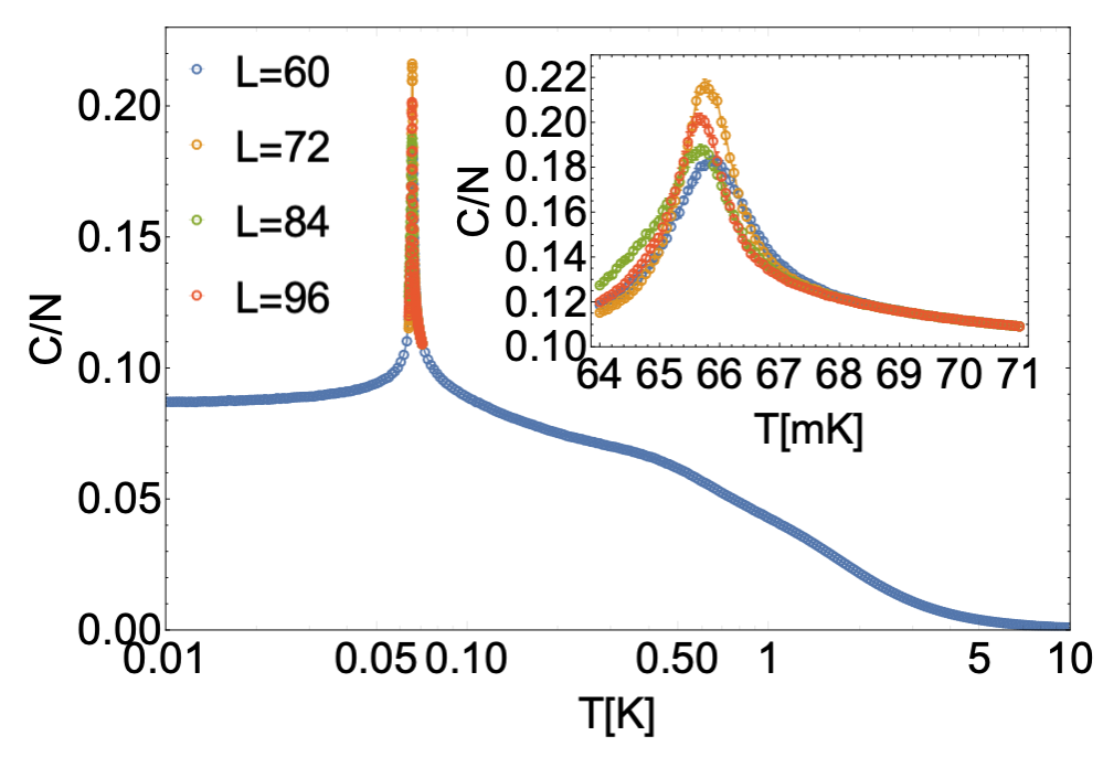
(a)

Figure 7: Normalized specific heat $c(T)=C(T)/N$ of spin–1/2 BBK model, for parameters taken from Ca₁₀Cr₇O₂₈ [cf. Table 2], with sharp peak at $T^{*}\ \approx 66\ \text{mK}$ signaling a phase transition into a low–temperature ordered state. Here $c(T)$ has been plotted on a log–linear scale, for direct comparison with Biswas and Damle (2018). Inset: detail of $c(T)$ near transition on a linear scale. Results are taken from classical Monte Carlo (MC) simulation of Eq. (1), for clusters with linear dimension $L=60,72,84,96$, as defined in the text.

In Fig. 7, we present MC results for normalized specific heat $c(T)=C(T)/N$ evaluated for parameters taken from Ca₁₀Cr₇O₂₈ [Table 2]. The dominant features of these results are a shoulder at $T\approx 500\ \text{mK}$, consistent with a crossover into a phase with collective spin fluctuations, and a sharp peak at $T^{*}\approx 66\ \text{mK}$, suggestive of a finite–temperature phase transition.

These temperature scales should be compared with the parameters of the BBK model [Table 2]. Both are less than the scale of the FM coupling within triangular plaquettes ($J_{22}\sim-2.3\ \text{K}$, $J_{21}\sim-6.5\ \text{K}$), but comparable with the interactions between spins in different plaquettes ($J_{0}\sim-69\ \text{mK}$, $J_{31}\sim 770\ \text{mK}$, $J_{32}\sim 950\ \text{mK}$). Thus we expect the thermodynamics of the BBK model to be determined by the collective excitations of groups of three spins on FM–coupled plaquettes — the regime described the effective honeycomb–lattice model, Eq. (6).

By analogy with earlier work on the honeycomb–lattice model, reviewed in Section II.7, we expect the peak at $T^{*}\approx 66\ \text{mK}$ to originate in a continuous transition into a state with broken lattice–rotation symmetry. Closer examination, shown in the inset of Fig. 7, reveals a nearly–symmetric peak, whose height has a weakly non–monotonic dependence of system size. The weakly non–monotonic behaviour seen in $c(T)$ presumably reflects the difficulty of simulating the critical behaviour of a system with dynamics based on triads of spins, using an update based on a single spin. Away from the critical region, i.e. for $T\neq T^{*}$, this does not present a problem. However it does prevent us from analysing the nature of any phase transition on the basis of $c(T)$ alone.

Instead, we now turn to an order parameter sensitive to the breaking of lattice rotation symmetry, of the type considered in Mulder et al. (2010); Okumura et al. (2010); Biswas and Damle (2018). We write this as

$$\phi = \sum_{{\bf r}\in\hexagon}\phi({\bf r})\;,$$ (9)

where the sum upon ${\bf r}$ runs over all sites of a honeycomb lattice (equivalently, all triangular plaquettes of the BBK lattice),

$$\phi({\bf r}) = \frac{1}{S^{2}}\left[{\bf S}_{A}({\bf r}){\bf S}_{B}({\bf r}+\hat{e}_{0})+\omega{\bf S}_{A}({\bf r}){\bf S}_{B}({\bf r}+\hat{e}_{1})\right.$$ (10)

$$\qquad\left.+\omega^{2}{\bf S}_{A}({\bf r}){\bf S}_{B}({\bf r}+\hat{e}_{2})\right]\;,$$

with

$$\omega = e^{i2\pi/3}\;,$$ (11)

and

$${\bf S}_{(A,B)}({\bf r})=\sum_{\delta=1}^{3}{\bf S}_{(A,B),\delta}({\bf r})\;,$$ (12)

is the total spin of an individual triangular plaquette, where the label A (B) corresponds to the lower (upper) plane of the BBK lattice. The vectors $\hat{e}_{i}$ defining the bonds between plaquettes in Eq. (10) are illustrated in Fig. 8.

In Fig. 9, we present results for the order–parameter susceptibility corresponding to Eq. (9),

$$\chi_{\phi}=\frac{1}{NT}\big{(}\langle|\phi|^{2}\rangle-\langle|\phi|\rangle^{2}\big{)}\ .$$ (13)

A sharp peak is found at $T^{*}\ \approx 66\ \text{mK}$, confirming that the anomaly found in specific heat [Fig. 7], is associated with a phase transition into a state with broken lattice–rotation symmetry. For system sizes $L\geq 60$, $\chi_{\phi}$ this peak shows a regular scaling with system size,

$$\chi_{\phi}\sim L^{\gamma/\nu}\qquad\gamma/\nu=1.61\pm 0.13\ .$$ (14)

Within error bars, this is consistent with the critical exponent of a three-state Potts model transition in 2D ($\gamma/\nu=26/15\approx 1.733$), as already discussed for the effective spin–3/2 honeycomb–lattice model Mulder et al. (2010); Biswas and Damle (2018). The critical temperature $T_{\text{c}}\approx 65\leavevmode\nobreak\ mK$ is also consistent with the value, found for the effective model Biswas and Damle (2018). Thus, while the BBK model of Ca₁₀Cr₇O₂₈, Eq. (1), is considerably more complicated than the effective honeycomb lattice model, Eq. (6), for parameters taken from experiment, Table 2, it exhibits exactly the same 3–state Potts transition, at a very similar temperature Biswas and Damle (2018).

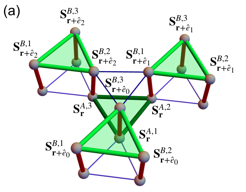
(a)

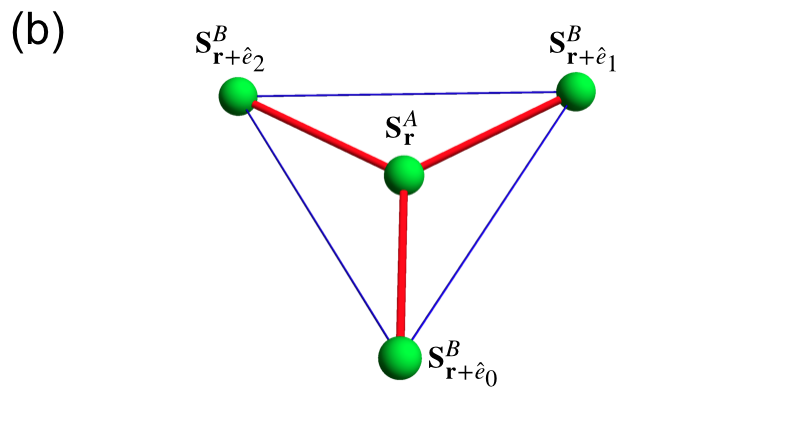
(b)

Figure 8: Illustration of labels used in definition of lattice–nematic order parameter, Eq. (13), associated with low–temperature ordered phase. (a) Four neighbouring triangular plaquettes of the BBK lattice, here shaded green. (b) Equivalent set of neighbouring sites within the honeycomb lattice considered in [Mulder et al., 2010; Biswas and Damle, 2018].

Building on the analogy with the honeycomb lattice, we can extend this analysis, from the parameters currently associated with Ca₁₀Cr₇O₂₈, to a parameter set equivalent to varying the ratio $J_{2}/J_{1}$ in Eq. (6). We do this by varying the ratio $x=J_{\sf eff}/J_{0}$, where $J_{\sf eff}$ [Eq.(7)] plays the role of $J_{2}$, and $J_{0}$ plays the role of $J_{1}$. Doing so, we arrive at the finite–temperature phase diagram shown in Fig. 6(a), where estimates of $T^{*}$ have been taken from the peak in heat capacity.

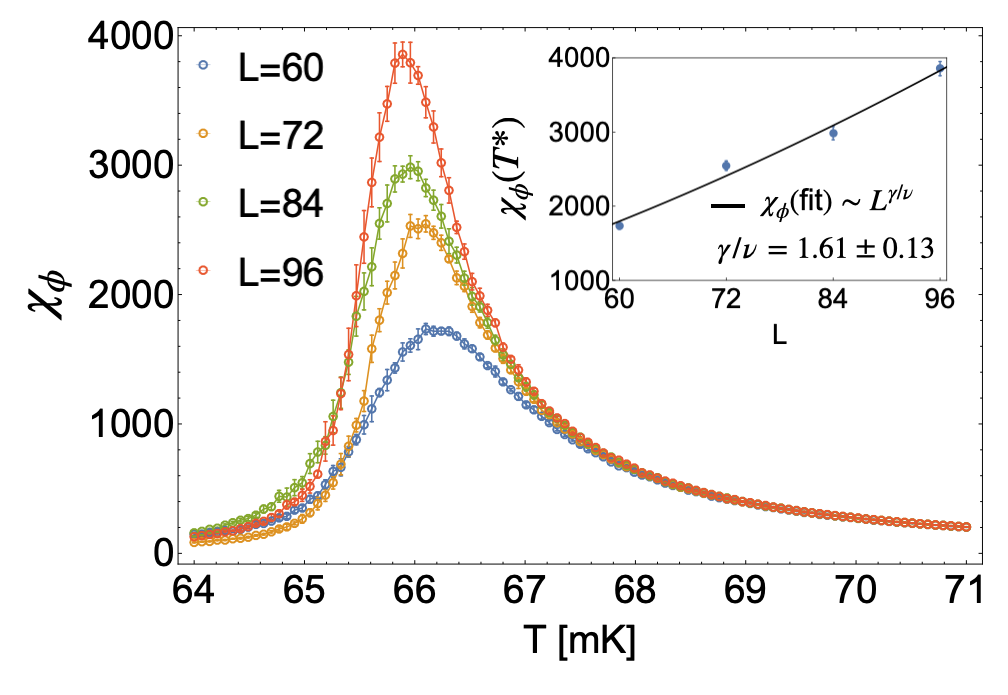
(a)

Figure 9: Order–parameter susceptibility associated with breaking of lattice–rotation symmetry, Eq. (13), showing evidence for a finite–temperature phase transition at $T^{*}\ \approx 66\ \text{mK}$. Inset: maximum value of susceptibility scales as $\chi_{\phi}\sim L^{\gamma/\nu}$, with critical exponent $\gamma/\nu=1.61\pm 0.13$. Within error bars, this is consistent with a three–state Potts transition ($\gamma/\nu=26/15\approx 1.733$), as discussed in [Mulder et al., 2010; Biswas and Damle, 2018]. Results are taken from classical Monte Carlo simulation of Eq. (1), for the same clusters used to determine heat capacity [Fig. 7].

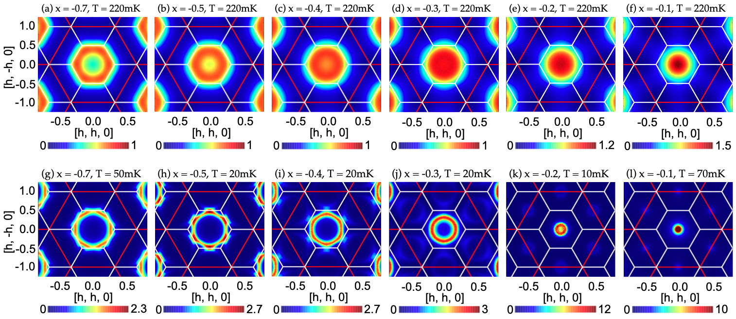
Figure 10: Evolution of the equal time structure factor $S({\bf q})$ as a function of $x=J_{\sf eff}/J_{0}$ [Eq. (7)], showing the impact of classical ground state degeneracy on correlations. (a)–(f) Results at $T=220\ \text{mK}$, within the spin–liquid phase, showing structured diffuse scattering, with correlations strongest on the zone boundary for $x<-0.5$. (g)–(l) Results at $T=T^{*}(x)+\epsilon$, just above the phase transition into an ordered state, showing the imprint of the different “ring” degeneracies. The transition from a “large” ring of degenerate spirals centered on $\Gamma$, to a “small” ring of degenerate spirals centered on $K$, occurs for $x=-0.5$. The asymmetry of scattering within the “small” ring, with suppression of weight at large $q$, reflects the form–factor of the BBK lattice. All results were obtained from classical Monte Carlo simulation of Eq. (1), for a cluster of linear dimension L = 60 (N = 21,600), with $J_{\sf eff}\equiv(J_{31}+J_{32})/2$, and other parameters taken from experiment [Table 2]. Magnetic scattering has the periodicity of the $4^{th}$ Brillouin zone, shown here with red lines.

We find that the ordering temperature, $T^{*}$, takes on a significantly higher value for parameters associated with a “small” ring of degenerate spiral states, for $x<-1/2$, than for parameters associated with a “large” ring of spiral ground states $-1/2<x<-1/6$ [cf. Fig. 5]. This appears to be consistent with transition temperatures found in earlier studies of the honeycomb lattice Mulder et al. (2010); Okumura et al. (2010); Biswas and Damle (2018). And, naively, it suggests that the entropy associated with the “large” ring of spirals, centered on $\Gamma$, is greater than the entropy associated with the small ring of spirals, centered on $K$. We return to this point in the context of the discussion of spin–liquid properties at finite temperature, below.

We note that, for $x>-1/6$, the anomaly seen in $c(T)$, and the corresponding estimate of a critical temperature in Fig. 6, should be associated with the onset of strong FM fluctuations, rather than lattice–symmetry breaking. However, as this case does not appear to have any bearing on the physics of Ca₁₀Cr₇O₂₈, we shall not consider it further here.

Published estimates of the exchange parameters of Ca₁₀Cr₇O₂₈ [Table 2] suggest a ratio of effective honeycomb–model interactions $x\approx 1.25$. This places Ca₁₀Cr₇O₂₈ within the region where the honeycomb model, Eq. (6), has a small ring of ground states centered on ${\bf q}=K$. However the relatively large uncertainty in the estimated values of $J_{1}$ and $J_{2}$, leads to considerable uncertainty in ratio, reflected in the error bar in the placement of Ca₁₀Cr₇O₂₈ in Fig. 6.

III.2 Correlations at finite temperatures

We next turn to the nature of spin correlations in the regime $T^{*}=66\ \text{mK}<T\lesssim 500\ \text{mK}$, where results for heat capacity are suggestive of collective behaviour. This is the range of temperatures where spin–liquid behaviour is most likely to be found in the classical limit of the BBK model. It is also the temperature regime relevant to published neutron scattering data for the quantum spin liquid in Ca₁₀Cr₇O₂₈ Balz et al. (2016, 2017a); Sonnenschein et al. (2019).

In Fig. 6, we show MC results for the equal–time structure factor $S({\bf q})$, calculated for parameters relevant to Ca₁₀Cr₇O₂₈. At a temperature of $T=220\ \text{mK}$, a broad “ring” of strong fluctuations is observed for ${\bf q}$ near to the Brillouin zone (BZ) boundary, with the strongest signal occurring near the $K$ points at BZ corners [Fig. 6(c)]. On lowering temperature to $T=90\ \text{mK}$, spectral weight is transferred from the zone boundary to diffuse, U–shaped structures at the zone corners [Fig. 6(d)].

Very similar results for $S({\bf q})$ have been found in large–N and classical MC calculations for the honeycomb–lattice model at $T=100\ \text{mK}$ Biswas and Damle (2018). The preponderance of scattering near the zone corners can be understood in terms of the “small” ring of classical ground states in the honeycomb–lattice model for $|J_{1}|\sim J_{2}$ [cf. Fig. 5]. Meanwhile the asymmetry visible in $S({\bf q})$ near the BZ corners reflects the form factor of the BBK lattice, which has the periodicity of the $4^{th}$ BZ, shown here with red lines.

When combined with the heat capacity [Fig. 7], these results suggest that fluctuations of spins in Ca₁₀Cr₇O₂₈ at temperatures $T\lesssim 500\ \text{mK}$ are both collective and highly structured, involving a set of q vectors which bears the imprint of nearby (classical) ground state degeneracies. This is consistent with a spin–liquid state at finite temperatures, where entropy predominates. And it is broadly similar to what has been observed in a number of models supporting “spiral spin liquids” Bergman et al. (2007); Okumura et al. (2010); Benton and Shannon (2015); Seabra et al. (2016); Buessen et al. (2018); Yao et al. (2021).

With this in mind, it is interesting to further explore the analogy with the honeycomb lattice model, by varying the values of the effective parameters $J_{1}$ and $J_{2}$, in such a way as to tune between different kinds of ground state degeneracies. In Fig. 10 we present results for the evolution of $S({\bf q})$ as a function of $x=J_{\sf eff}/J_{0}$, [Eq. (7)], at temperatures well within the spin–liquid phase, and just above the transition into the ordered ground state [cf. Fig. 6]. We consider a range of parameters $-0.7\leq x\leq-0.1$ which span both the “large” and “small’ ring degeneracies of the honeycomb lattice model [cf. Fig. 5].

At $T=220\ \text{mK}$ (upper panels), for $x<-0.3$, correlations are strongest near to the BZ boundary. Meanwhile, for $x\geq-0.3$, they start to resemble the “pancake–liquid” identified in Okumura et al. (2010), with stronger scattering in the zone center. At temperatures just above the peak observed in specific heat, $T=T^{*}+\epsilon$ (lower panels), the imprint of the ground–state degeneracy of the equivalent honeycomb–lattice model, Eq. (6), is evident in rings of high intensity. These are centered on $K$ for $x<-0.5$ and on $\Gamma$ for $x>-0.5$ [cf. Fig. 5].

Returning to experimentally–motivated parameters, $x=1.25$, it is interesting to compare these results with published calculations of the structure factor of the BBK model coming from PFFRG Balz et al. (2016) and phenomenological parton approaches Sonnenschein et al. (2019). PFFRG results for the static structure factor $S({\bf q},\omega=0)$ at $T=0$ suggest strong correlations near to the BZ boundary, with additional weight near to zone corners $K$ Balz et al. (2016). This is qualitatively very similar to MC results at $T=220\ \text{mK}$, within the spiral spin liquid phase [Fig. 6(c)]. The $T=0$ parton phenomenology, meanwhile, shows energy–dependent ring—like structure in $S({\bf q},\omega)$, centered on $\Gamma$ Sonnenschein et al. (2019). And to meaningfully compare with this, it is necessary to analyse dynamics.

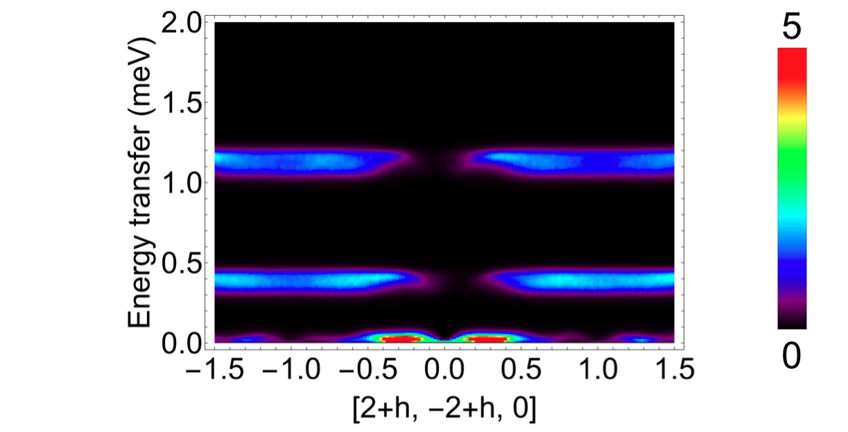
(a) $\tilde{S}({\bf q},\omega),B=0$

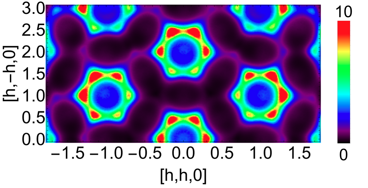
(b) $\tilde{S}({\bf q},\omega=0.01\ \text{meV})$

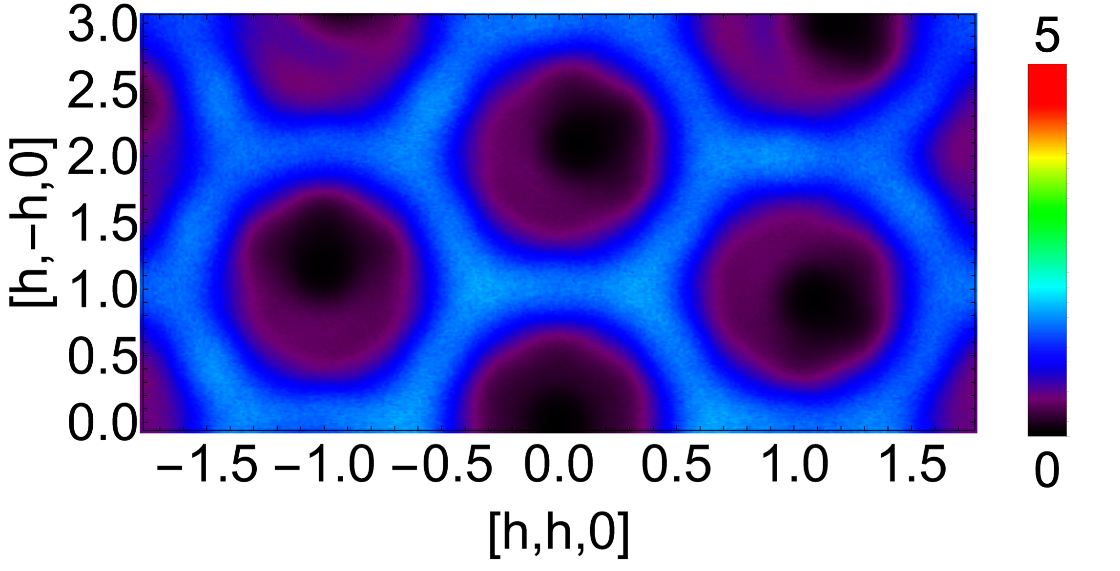
(c) $\tilde{S}({\bf q},\omega=0.35\ \text{meV})$

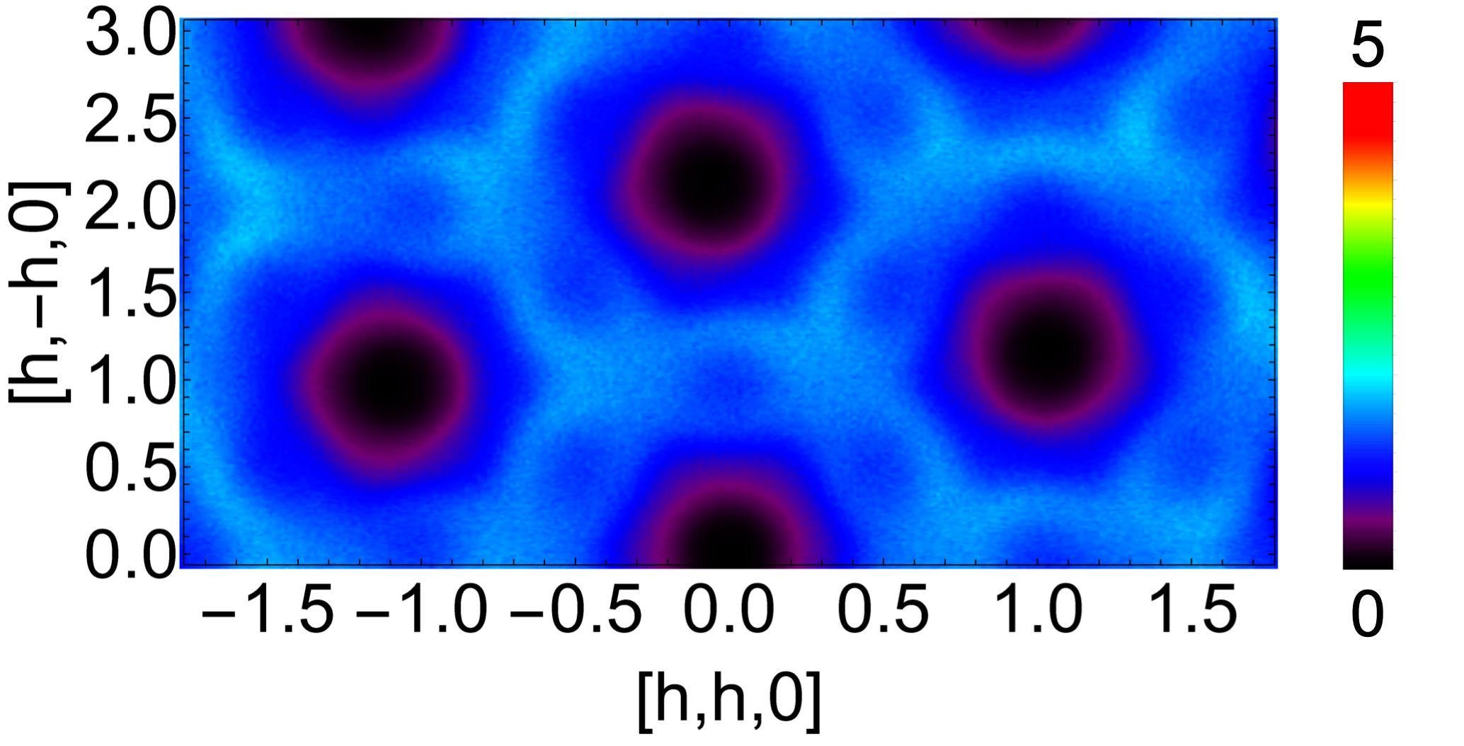
(d) $\tilde{S}({\bf q},\omega=1.13\ \text{meV})$

Figure 11: Spin dynamics in zero field, showing the different correlations found on different energy scales. The first moment of the dynamical structure factor $\tilde{S}({\bf q},\omega)$ [Eq. (17)] was obtained from molecular dynamics (MD) simulation of the BBK model, Eq. (1), at $T=220\ \text{mK}$, for a cluster of linear dimension $L=48$ ($N=13,824$), with parameters taken from Experiment [Table. 2]. Results are presented with energy resolution of FWHM $=0.02\ \text{meV}$, and no Cr⁵⁺ form factor.

IV Dynamical properties of ${\cal H}_{\sf BBK}$

The thermodynamic properties of the BBK model, reported in Section III, are consistent with the experimental observation that Ca₁₀Cr₇O₂₈ enters a spin–liquid state at temperatures $T\lesssim 500\ \text{mK}$. To learn more about this spin liquid, we now turn to dynamical simulations. These will provide us with a basis for comparison with inelastic neutron scattering (INS) experiments, which reveal dynamics at a range of different energy scales Balz et al. (2016, 2017a); Sonnenschein et al. (2019).

We adopt a (semi–)classical approach, in which spin configurations are drawn from a Boltzmann distribution, generated by MC simulation, and then evolved according to the Heisenberg equation of motion Moessner and Chalker (1998b); Conlon and Chalker (2010); Taillefumier et al. (2014)

$$\frac{d{\bf S}_{i}}{dt}=\frac{i}{\hbar}[{\bf S}_{i},\mathcal{H}_{\sf BBK}]=\bigg{(}\sum_{j}J_{ij}{\bf S}_{j}-B^{z}\hat{\mathbf{z}}\bigg{)}\times{\bf S}_{i}\;.$$ (15)

This approach to the dynamics of spin liquids was popularised by Moessner and Chalker Moessner and Chalker (1998a, b), who dubbed it “Molecular Dynamics” (MD) simulation, by analogy with Monte Carlo techniques used in the simulation of fluids.

We note that this “MD” approach has much in common with the numerical solution of the Landau–Lifschitz–Gilbert equation Gilbert (2004)

$$\frac{\partial{\bf M}}{\partial t}=-\gamma^{*}{\bf M}\times{\bf H}-\frac{\alpha}{M}{\bf M}\times\frac{\partial{\bf M}}{\partial t}\;.$$ (16)

However there are also some important differences, notably the use of microscopic spin variables ${\bf S}_{i}$, rather than a course–grained magnetisation ${\bf M}$; the absence of a phenomenological damping term $\alpha$; and the use of an ensemble of initial states drawn from classical MC simulation. Further details of our numerical methods can be found in Appendix A.

In the context of Ca₁₀Cr₇O₂₈, the great advantage of the MD approach is that it is possible to simulate the finite–temperature spin dynamics of clusters of more than N=$10,000$ spins, facilitating a quantitative comparison with experiment, even in the absence of magnetic order, and in models which would be subject to a sign problem in quantum Monte Carlo simulation. And even though the MD method fails to take into account either entanglement, or quantum statistics of excitations, it has previously been found to give a good account of the qualitative features of quantum models for problems as diverse as the Kitaev model Samarakoon et al. (2017); quantum spin ice Taillefumier et al. (2017); the spin liquid phase of NaCaNi₂F₇ Zhang et al. (2019), and the semi–classical dynamics of spin density waves Chern et al. (2018).

IV.1 Comparison of simulation with experiment

We start by comparing simulations of dynamics carried out in the spin–liquid phase of the BBK model with results found in experiment. Key results have already been summarised in Fig. 2, where we show MD results for the dynamical structure factor $S({\bf q},\omega)$, side-by-side with results from INS Balz et al. (2016). To facilitate comparison, simulation results have been convoluted with a Gaussian mimicking experimental resolution, and a magnetic form factor appropriate for a Cr⁵⁺ ion [cf. Appendix C]. Both experiment and theory show rings of scattering at low energy, consistent with the discussion in Section III.2. They also agree on a broad network of scattering at intermediate to high energy, which is concentrated near to the zone boundary, with hints of “bow–tie” like structures near to $(1,0,0)$. (Bright “spots” seen in INS near to zone centers represent scattering from phonons, and do not form part of the magnetic signal Balz et al. (2016)).

Clearly, the MD simulations capture important elements of the physics of Ca₁₀Cr₇O₂₈. Moreover, the “ring” found at low energies in MD simulation corresponds very closely to the ring found in the static structure factor $S({\bf q},\omega=0)$ in PFFRG calculations Balz et al. (2016), and a related parton phenomenology Sonnenschein et al. (2019). This suggests that important aspects of quantum treatments of the BBK model are reproduced. The question which remains, is what this tells us about the nature, and origin, of the spin-liquid in Ca₁₀Cr₇O₂₈ ?

IV.2 Evolution of spin configurations in spin liquid as a function of time [First Animation]

One very direct route into this question is to look at the evolution of spin configurations in real–space, as a function of time. This is accomplished in the First Animation provided in the Supplementary Material fir . The simulations shown in this animation were carried out for $N=5400$ spins at a temperature of $T=220\ \text{mK}$, deep inside the classical spin–liquid regime [Fig. 6(a)], where the equal–time structure factor $S({\bf q})$ reveals a diffuse “ring” structure [Fig. 6(c)]. As the Animation shows, the spins continue to fluctuate, even at this low temperature. And on closer inspection, the simulation reveals that the spins exhibit both slow and fast dynamics, and they have very different characters. The slow precession of locally collinear spins is mixed with fast fluctuations of seemingly-uncorrelated spins. For clarity, spins which rotate quickly have been coloured red, while spins which rotate slowly have been coloured green; further details of the animation can be found in Appendix B.

IV.3 Correlations as a function of energy and momentum

To better understand the dynamics on different time scales observed in the spin liquid, we now return to the dynamical structure factor. This time however, in order to compensate for the classical statistics of the MC simulations, we do not plot the dynamical structure factor $S({\bf q},\omega)$ directly, but rather its first moment, divided by the temperature at which the simulations are carried out Pohle et al. (2017); Zhang et al. (2019); Remund et al. :

$$\tilde{S}({\bf q},\omega)=\frac{1}{2}\frac{\omega}{k_{B}T}S_{\sf MD}({\bf q},\omega)\;.$$ (17)

Further details of this approach can be found in Appendix A.3.

In Fig. 11a, we present results for parameters equivalent to the First Animation, for a cluster of $N=13,824$ spins. Results are shown for the $[2+h,-2+h,0]$ plane in reciprocal space, considered in Balz et al. (2017a); the atomic form factor has been set equal to unity, in order to make it easier to distinguish correlations over a broad area of reciprocal space. Bands of excitations are observed with three different energy scales, $\omega\sim 0.0$, $0.4$ and $1.1\ \text{meV}$. The upper bands are diffuse, with no sharp features, and only very weakly dispersing, suggesting that excitations are nearly localised. The characteristic energy scale of the upper (lower) “flat” mode is set by the ferromagnetic coupling strengths $J_{22}$ ($J_{21}$), reflecting the transition from a high–spin to a low–spin state on an individual triangular plaquette. Each “mode” comprises two distinct bands, with band–width determined by the antiferromagnetic coupling $J_{31}$ ($J_{32}$).

These quasi–localised excitations are a robust feature of the bilayer breathing kagome (BBK) model of Ca₁₀Cr₇O₂₈, and are also seen in quantum simulations Shimokawa et al. (tion). They are an echo, at finite energy, of the “Coulombic” spin–liquid found in the Heisenberg antiferrmognet on a Kagome lattice, and support both “pinch–point” and “half–moon” features in neutron scattering Yan et al. (2018). As required for a rotationally symmetric Hamiltonian like Eq. (1), spectral weight vanishes for ${\bf q}=0$ at all finite $E$. The lower band, meanwhile, is much more structured, with spectral weight predominantly found in high-intensity patches centered around ${\bf q}=0$.

In Fig. 11b, we show a cross section through $S({\bf q},\omega)$ for $\omega=0.01\ \text{meV}$, once again choosing our plane in reciprocal space to match equivalent results in Balz et al. (2016, 2017a). The high-intensity patches centered around ${\bf q}=0$ are immediately recognisable as the “ring” observed in $S({\bf q})$ [Fig. 6(c)] with strong intensity near the K-points at the zone-corners. And further “rings” are observed at $(2,0,0)$, etc., reflecting the periodicity of the 4^th BZ. These are connected by a diffuse web of scattering which preserves the overall 6-fold rotation symmetry of the lattice.

In Fig. 11c, we present equivalent results for $\omega=0.35\ \text{meV}$, the characteristic energy scale of the intermediate band of excitations in Fig. 11a. The structure observed is utterly different. The “Ring” like features found in the lower band are conspicuously absent, being replaced by a broad web of correlations tracking the boundary of the extended (4^th) BZ. Superimposed on this web, we find a blurred but regular array of triangular features, which meet to form “bow–ties” centered on reciprocal lattice points $(1,0,0)$, etc.

Finally, in Fig. 11d, we present results for $\omega=1.13\ \text{meV}$, the characteristic energy scale of the highest band of excitations in Fig. 11a. Here once again we find a broad web of correlations tracking the boundary of the extended BZ. And once again this has structure superimposed on it. But at this particular energy, that structure takes the form of crescent features centered on the same reciprocal lattice vectors as the bow–ties described above, i.e. $(1,0,0)$, etc.

IV.4 Evolution of spin configurations in spin liquid as a function of time, revisited [Second Animation]

From these results it is clear that i) dynamics occur on three different times scales, and ii) that the dynamics on long time scales (low–energy band) is qualitatively different from that on short time scales (intermediate– and high–energy bands). With these lessons in mind, we can revisit the time–evolution of spin configurations in real space, and apply a filter to separate dynamics into slow, intermediate and fast bands of excitations.

In the Second Animation provided in the Supplementary Material sec , we show the separate time evolution of slow, intermediate and fast spin fluctuations, in three different panels. Viewed at “normal” speed, only the slow fluctuations are clearly intelligible, as collective rotation of spins which are locally collinear on each of the ferromagnetic plaquettes of the BBK lattice. To make comparison easier, in the second part of the Animation, we adjust the “clock” for each panel, speeding up the slow fluctuations, and slowing down the fast ones, such that all processes occur at (roughly) the same subjective speed. At the same time, we reintroduce the color cues for speed, with rapdily–rotating spins appearing in red. Further details of the entire procedure are given in Appendix B.

Once the time series coming from simulations has been processed in this way, the contrasting character of excitations at different timescales is obvious. Slow fluctuations, once speeded up, are more obviously collective, with triads of spins on neighbouring FM plaquettes moving in unison. Intermediate and fast fluctuations, meanwhile, are seen to have the same character, and to comprise two, seemingly uncorrelated processes. The first of these is the collective rotation of spins on the AF plaquettes of the lattice, within each of which they (approximately) maintain a condition of net zero spin, familiar from the Kagome–lattice AF Chalker et al. (1992); Zhitomirsky (2008); Taillefumier et al. (2014). Superimposed on this are extremely fast spin–flips of individual spins, which appear to propagate in pairs around the lattice.

In summary, the dynamics of the classical spin liquid found in the BBK model of Ca₁₀Cr₇O₂₈ are complicated, unusual, and interesting. The degree of complexity is perhaps not a surprise, given the large unit cell and low–symmetry of the BBK lattice. None the less, it is possible to interpret simulation results for dynamics, through a combination of spectral functions, and animations of real–space dynamics. What makes the dynamics unusual, is that they appear to be qualitatively different on different timescales, and to combine aspects of two very different spin liquids, the “spiral spin liquids” studied in models with complex competing interactions Bergman et al. (2007); Okumura et al. (2010); Benton and Shannon (2015); Seabra et al. (2016); Buessen et al. (2018); Yao et al. (2021), and the celebrated spin liquid found in Kagome lattice AF Chalker et al. (1992); Zhitomirsky (2008); Robert et al. (2008); Taillefumier et al. (2014). This multiple–scale dynamics would be interesting by itself, but what makes it compelling is that many aspects of these dynamics have already been seen in INS measurements on Ca₁₀Cr₇O₂₈, a point which we return to in Section VII, below.

V Thermodynamic properties of BBK model in applied magnetic field

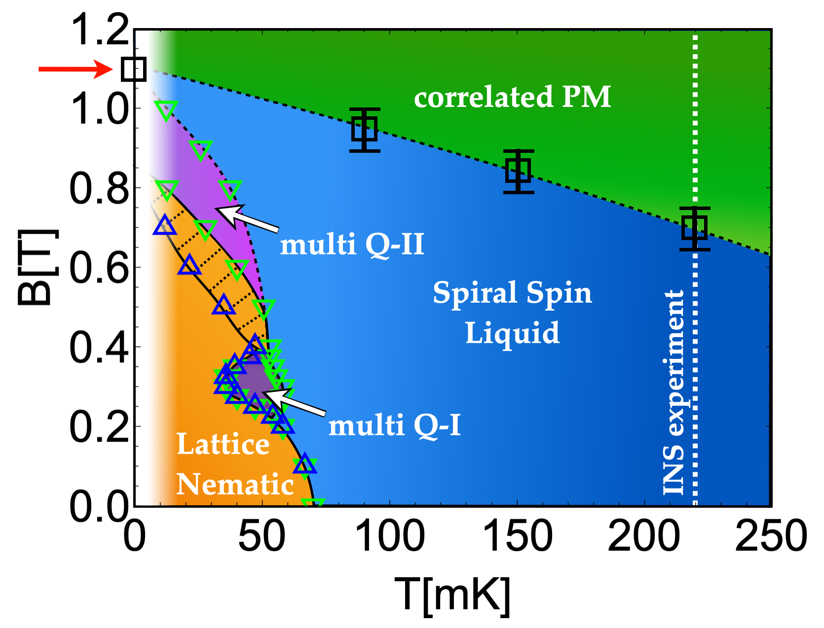
(a)

Figure 12: Low–temperature phase diagram found in classical Monte Carlo simulations of the bilayer breathing Kagome (BBK) model of Ca₁₀Cr₇O₂₈, for a cluster of $N=1944$ spins. The closing of a gap to transverse spin excitations at a critical field $B\lesssim 1\ \text{T}$ converts the correlated paramagnet into a spiral spin liquid, with characteristic “ring” in $S({\bf q})$ [Section VI]. A small domain of lattice–nematic and multiple–q orders is found at temperatures below $70\ \text{mK}$ [Section V]. Results are taken from classical Monte Carlo simulation of ${\mathcal{H}}_{\sf BBK}$ [Eq. (1)], as described in Section V. The temperature associated with simulation results for dynamics, $T=220\ \text{mK}$, [Section IV, Section VI] is shown with a white dashed line [cf. Fig. 2]. The critical fields indicating the closing of the energy gap to spin excitations, as obtained from MD simulations at $T=90,150,220\ \text{mK}$ [cf. Fig 22], and linear spin wave theory at $T=0$, are shown with black squares ($\square$). Low–temperature anomalies in specific heat $c(T)$ are denoted with green triangles ($\triangledown$); peaks in the nematic order parameter susceptibility [cf. Eq. (20)], with blue triangles ($\triangle$).

Studies of Ca₁₀Cr₇O₂₈ in applied magnetic field have already proved very useful in, e.g. providing estimates of the microscopic exchange parameters of the BBK model [cf. Section II.5]. In what follows we use magnetic field as a tool to learn more about the nature and origin of its spin–liquid phase, starting with the thermodynamic properties found in MC simulations, for parameters corresponding to Ca₁₀Cr₇O₂₈ [Table 2]. Key results are summarised in the phase diagram, Fig. 12.

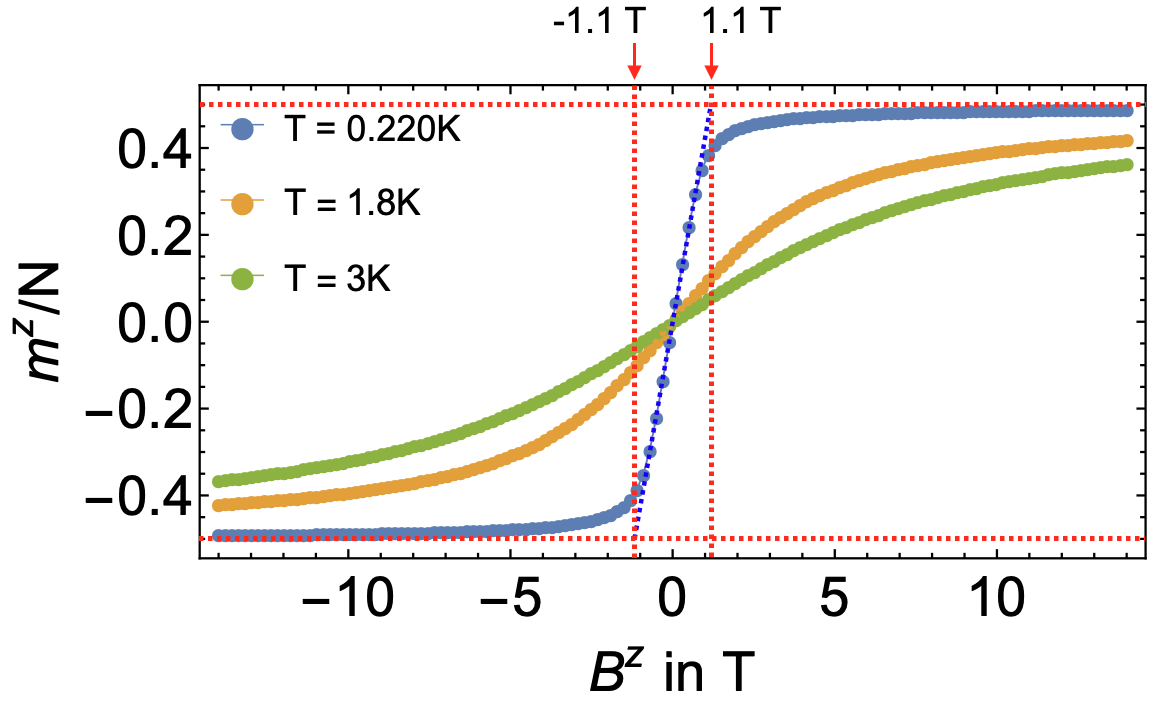
(a)

Figure 13: Magnetisation of the classical BBK model of Ca₁₀Cr₇O₂₈ as a function of magnetic field, showing strong dependence on temperature. At the lowest temperatures, magnetisation approaches saturation, $|m^{z}|\to 0.5$ (horizontal dashed line) for $|B|>1.1\ \text{T}$, the saturation field predicted by linear spin-wave theory at $T=0$ (vertical dashed line). At higher temperatures very large fields are needed to saturate the magnetization, consistent with a high density of thermally–excited spin excitations. Results are taken from classical Monte Carlo simulation of ${\mathcal{H}}_{\sf BBK}$ [Eq. (1)], for a cluster of linear dimension L = 48 (N = 13,824), with parameters taken from experiment [Table 2].

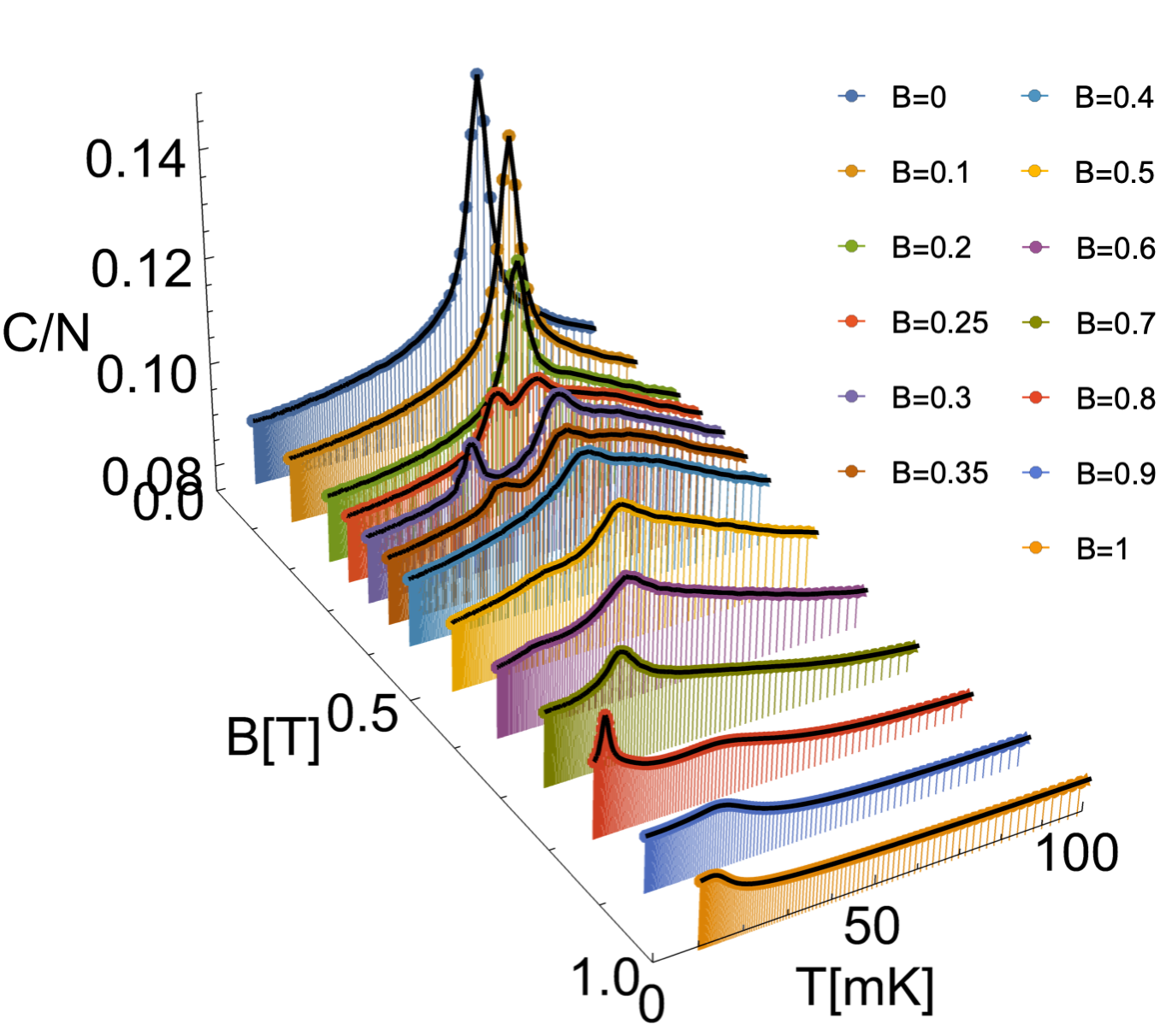
(a)

Figure 14: Heat capacity of BBK model of Ca₁₀Cr₇O₂₈ as a function of magnetic field. Results are shown for $T<100\ \text{mK}$, with magnetic field ranging from $B=0\ \text{T}$ [blue curve, top of panel] to $B=1.0\ \text{T}$ [orange curve, bottom of panel]. A number of different anomalies are observed, distinguishing different (quasi–)ordered phases, as described in the main text. Results are taken from classical Monte Carlo simulation of ${\mathcal{H}}_{\sf BBK}$ [Eq. (1)], for a cluster of linear dimension L = 18 (N = 1944), with parameters taken from experiment [Table 2].

V.1 Magnetisation in field

We consider first the magnetisation, $m(B)$. In Fig. 13 we show MC simulation results for $m(B)$, at temperatures of $T=220\ \text{mK}$ (within the spin liquid) and $T=1.8\ \text{K}$ and $3\ \text{K}$, (within a high-temperature paramagnetic phase) [cf. Fig. 12]. MD simulations find a spin liquid which is gapless in zero field [Fig. 11a], consistent with both expectations for an O(3)–invariant classical model, and experiment on Ca₁₀Cr₇O₂₈ Balz et al. (2016). In keeping with this, simulations at $T=220\ \text{mK}$, reveal that the spin liquid has a finite magnetic susceptibility, with a nearly linear behavior of $m(B)$ up to a field $B\sim 0.7\ \text{T}$. Interestingly, the susceptibility within the spin liquid at this temperature is very close to the value found by dividing the saturated moment $m=0.5$ by the zero–temperature saturation field found in spin wave theory, $B=1.1\ \text{T}$ (vertical dashed line). For $B>0.7\ \text{T}$, $m(B)$ is more “rounded”, and tends towards the full saturated moment (horizontal dashed line) for $B\approx 10\ \text{T}$.

Results for $m(B)$ in the paramagnetic phase, for $T=1.8\ \text{K}$ and $3\ \text{K}$, also show a finite magnetic susceptibility, but no hint of saturation up to the highest fields simulated. We note that the failure of the magnetisation to saturate at these temperatures is an artifact of classical statistics, and is not reproduced by quantum simulations Shimokawa et al. (tion).

V.2 Heat capacity in field

More can be learned by looking at the heat capacity, $c(T)$ under applied magnetic field. Results taken from MC simulations are shown in Fig. 14. Many of the large–scale features observed in the absence of field persist; in particular, the broad shoulder at $T\sim 500\ \text{mK}$ (not shown) is little affected by fields $B\lesssim 1\ \text{T}$, suggesting that spin excitations below this temperature scale remain collective. And, for magnetic fields $B\lesssim 0.7\ \text{T}$, we can identify a sharp peak in specific heat in $c(T)$ which connects smoothly with the phase transition from spin–liquid to $Z_{3}$ lattice nematic observed in zero field [Fig. 7].

However, for fields $B\gtrsim 0.2\ \text{T}$, new features start to emerge. In particular, for $0.225<B<0.375\ \text{T}$, the sharp anomaly in $c(T)$ associated with the onset of lattice–rotation symmetry splits into two peaks. Moreover for $B\gtrsim 0.5\ \text{T}$, a further weak anomaly (shoulder) becomes visible in $c(T)$, at a temperature higher than any sharp peak. This new feature moves steadily to lower temperature with increasing field, finally interpolating to $T\to 0$ at the critical field found in spin wave theory $B_{c}=1.1\ \text{T}$.

These features divide the low–temperature phase diagram into several distinct regions, which we characterise below.

V.3 Evolution of $Z_{3}$ lattice–nematic order in field

We first consider the phase found at low temperature and low field, which connects with the $Z_{3}$ lattice–nematic order found for $B=0$. The order parameter for lattice–nematic order, Eq. (9), can be generalised for finite magnetic fields, as

$$\phi_{\nu} = \sum_{{\bf r}\in\hexagon}\phi_{\nu}({\bf r})\;,$$ (18)

where

$$\phi_{\parallel}({\bf r}) = \frac{1}{S^{2}}\left[S^{z}_{A}({\bf r})S^{z}_{B}({\bf r}+\hat{e}_{0})+\omega S^{z}_{A}({\bf r})S^{z}_{B}({\bf r}+\hat{e}_{1})\right.$$ (19)

$$\qquad\left.+\omega^{2}S^{z}_{A}({\bf r})S^{z}_{B}({\bf r}+\hat{e}_{2})\right]\;,$$

$$\phi_{\perp}({\bf r}) = \frac{1}{S^{2}}\left[{\bf S}^{\perp}_{A}({\bf r}){\bf S}^{\perp}_{B}({\bf r}+\hat{e}_{0})+\omega{\bf S}^{\perp}_{A}({\bf r}){\bf S}^{\perp}_{B}({\bf r}+\hat{e}_{1})\right.$$ (20)

$$\qquad\left.+\omega^{2}{\bf S}^{\perp}_{A}({\bf r}){\bf S}^{\perp}_{B}({\bf r}+\hat{e}_{2})\right]\;,$$

where the conventions for labelling sites within the plaquettes A and B are given in Fig. 8, and

$${\bf S}^{\perp}({\bf r}) = (S^{x}({\bf r}),S^{y}({\bf r}))$$ (21)

We find that the dominant contribution comes from $\phi_{\perp}$, and the associated order parameter susceptibility, $\chi^{\perp}_{\phi}(T)$, shows a sharp peak which tracks the anomaly in $c(T)$, confirming that this originates in the breaking of lattice–rotation symmetry [Fig. 15a].

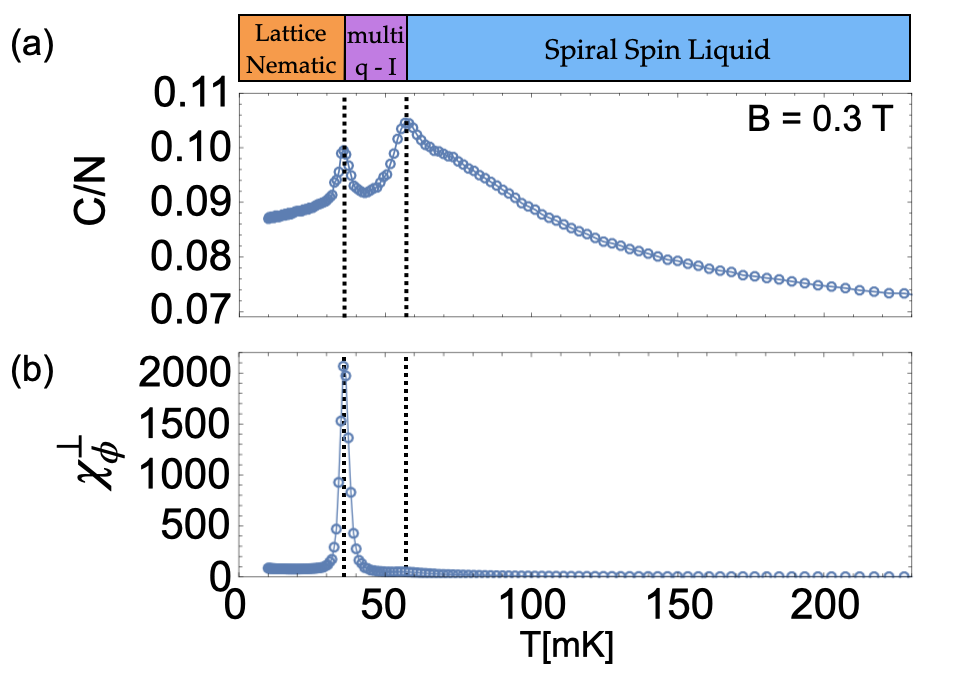
(a)

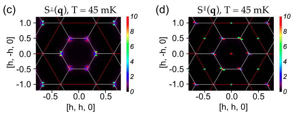
(b)

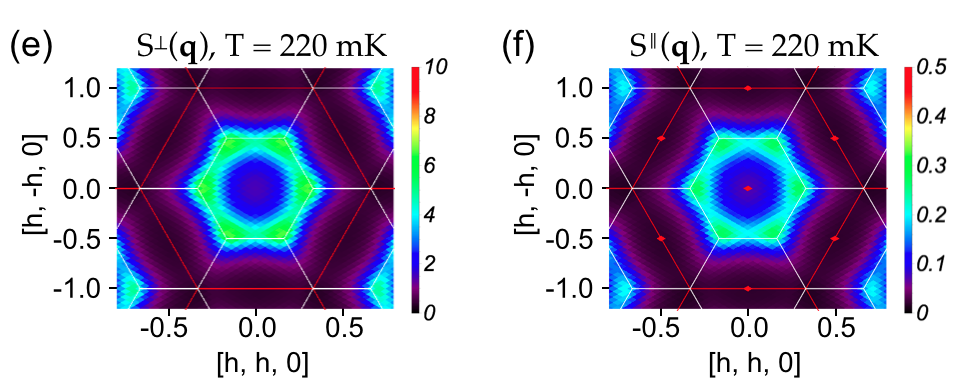
(c)

Figure 15: Thermodynamic properties of BBK model of Ca₁₀Cr₇O₂₈ at $B=0.3$T showing evidence for a multiple–q state separating the $Z_{3}$–ordered lattice–nematic from the spiral spin liquid. (a) Heat capacity $C(T)/N$, showing distinct peaks at $35(2)\ \text{mK}$ and $58(2)\ \text{mK}$. (b) Susceptibility associated $Z_{3}$ order parameter, $\chi^{\perp}_{\phi}(T)$ [Eqs. (13), (20)], showing sharp peak at $35(2)\ \text{mK}$. (c) Transverse structure factor $S_{\perp}({\bf q})$ at $T=45$mK, within the “multiple–q (I)” phase, showing a matrix of points associated with a multiple–q state near to zone corners. (d) Longitudinal structure factor $S_{\parallel}({\bf q})$ at the same temperature. Zone-center peaks reflect the finite magnetisation of the system. (e) Transverse structure factor $S_{\perp}({\bf q})$ at $T=220$mK, showing diffuse scattering features, as observed in zero field [see Fig.6 (c)]. (f) Longitudinal structure factor $S_{\parallel}({\bf q})$ at $T=220$mK, showing the same diffuse scattering features as in (e) with additional Bragg peaks at Brillouin zone centers, accounting for spin polarization in field. Results are taken from classical Monte Carlo simulation of the BBK model Eq. (1), for a cluster of linear dimension L = 18 (N = 1944), with parameters taken from experiment [Table 2]. To distinguish multiple–q states, simulations have been performed in absence of parallel tempering [Appendix  A].

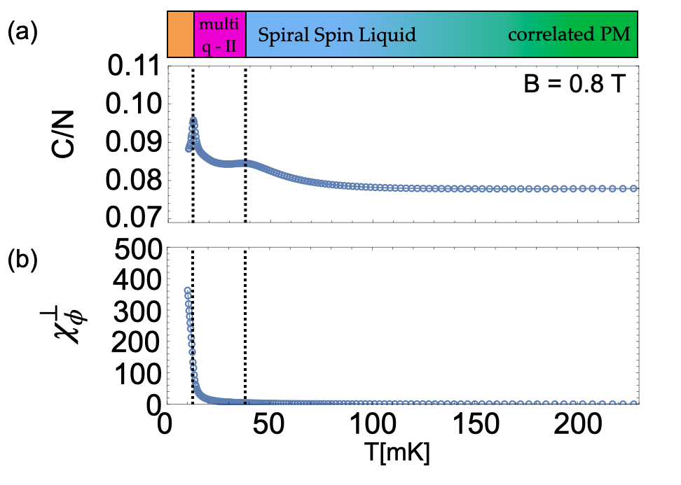
(a)

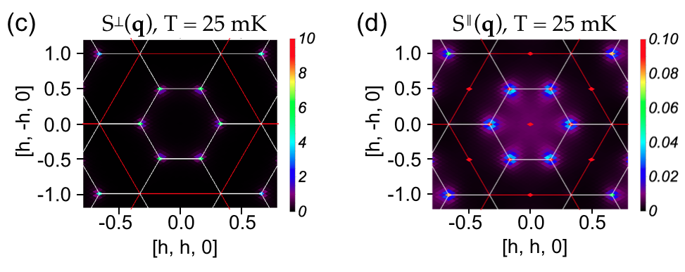
(b)

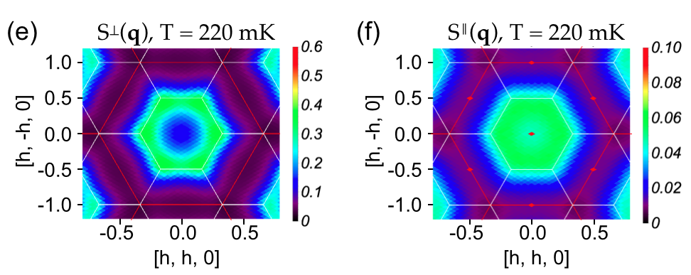
(c)

Figure 16: Thermodynamics of BBK model of Ca₁₀Cr₇O₂₈ at $B=0.8$T. (a) Heat capacity $C(T)/N$, showing shoulder around $\sim 40\ \text{mK}$, associated with the onset of the “multiple–q (II)” phase, and sharp peak at $11(2)\ \text{mK}$, marking phase transition into $Z_{3}$ lattice nematic. The transition between the correlated paramagnet and spiral spin liquid is not accompanied by any visible anomaly in $C(T)/N$. (b) Susceptibility associated with $Z_{3}$ order parameter, $\chi^{\perp}_{\phi}(T)$ [Eqs. (13), (20)], showing sharp peak at $11(2)\ \text{mK}$. (c) Transverse structure factor $S_{\perp}({\bf q})$ at $T=25$mK within the “multiple–q (II)” phase, showing points associated with a multiple–q state near to zone corners. (d) Longitudinal structure factor $S_{\parallel}({\bf q})$ at the same temperature. (e) Transverse structure factor $S_{\perp}({\bf q})$ at $T=220$mK, showing diffuse scattering features, as observed in Fig.15(e). (f) Longitudinal structure factor $S_{\parallel}({\bf q})$ at $T=220$mK, showing qualitatively different features, compared to Fig.15(f), emphasizing the correlated nature of the paramagnetic phase. Results are taken from classical Monte Carlo simulation of the BBK model Eq. (1), for a cluster of linear dimension L = 18 (N = 1944), with parameters taken from experiment [Table 2]. To facilitate the understanding of order, measurements have been performed in absence of parallel tempering.

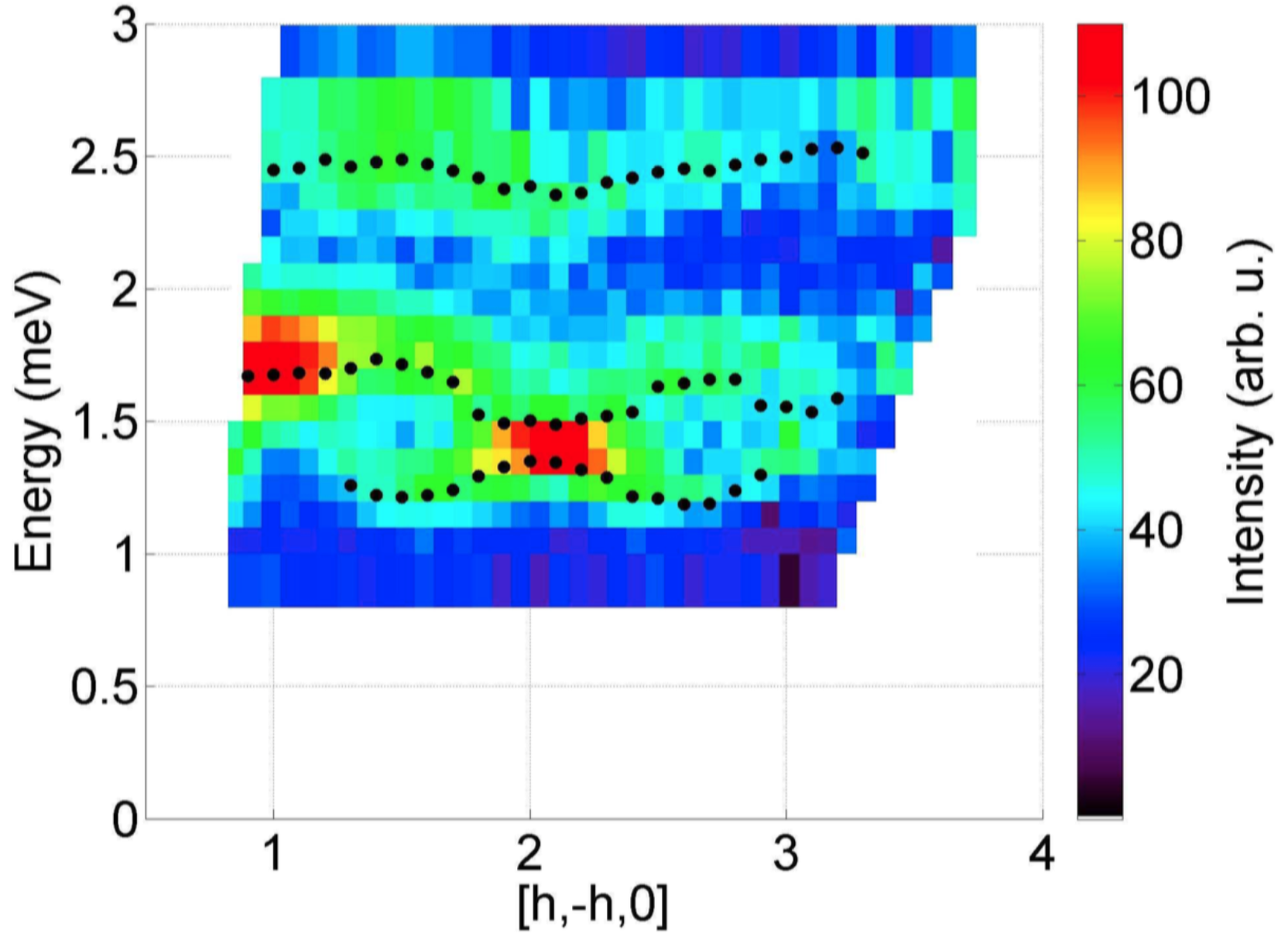
(a) INS, T = 90mK

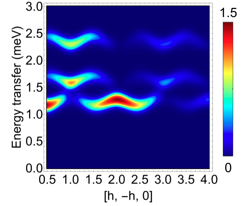
(b) $S^{\sf LSW}_{\sf T=0}({\bf q},\omega)$

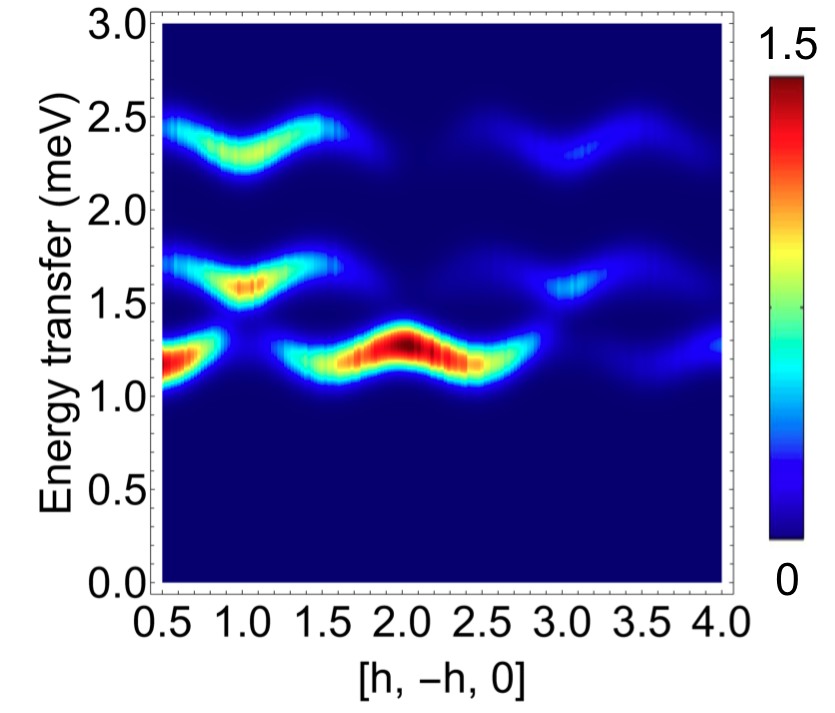
(c) $\tilde{S}^{\sf MD}_{\sf T=10mK}({\bf q},\omega)$

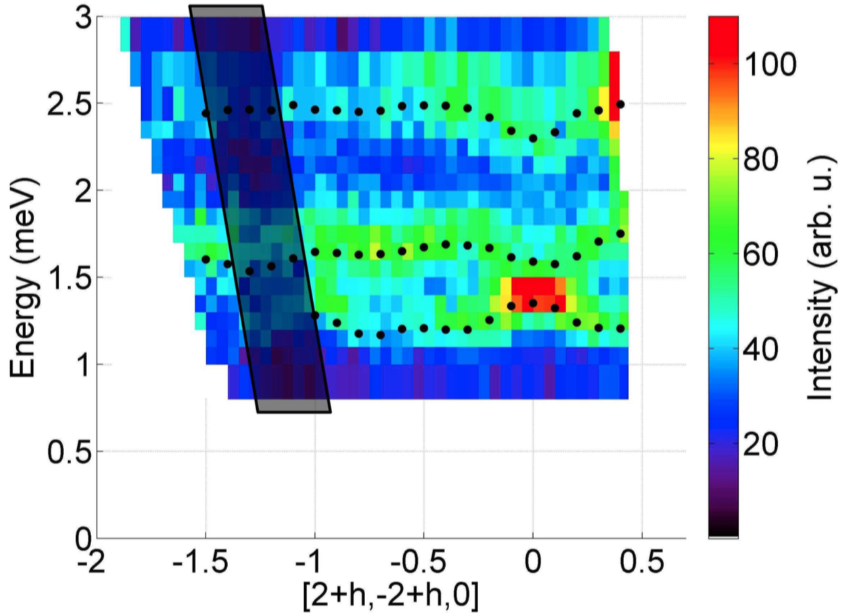
(d) INS, T = 90mK

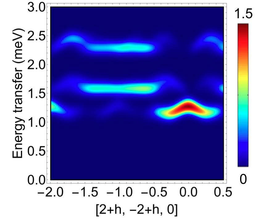
(e) $S^{\sf LSW}_{\sf T=0}({\bf q},\omega)$

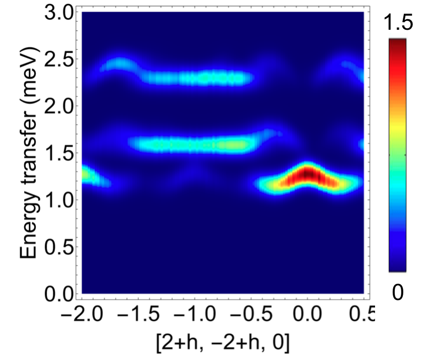
(f) $\tilde{S}^{\sf MD}_{\sf T=10mK}({\bf q},\omega)$

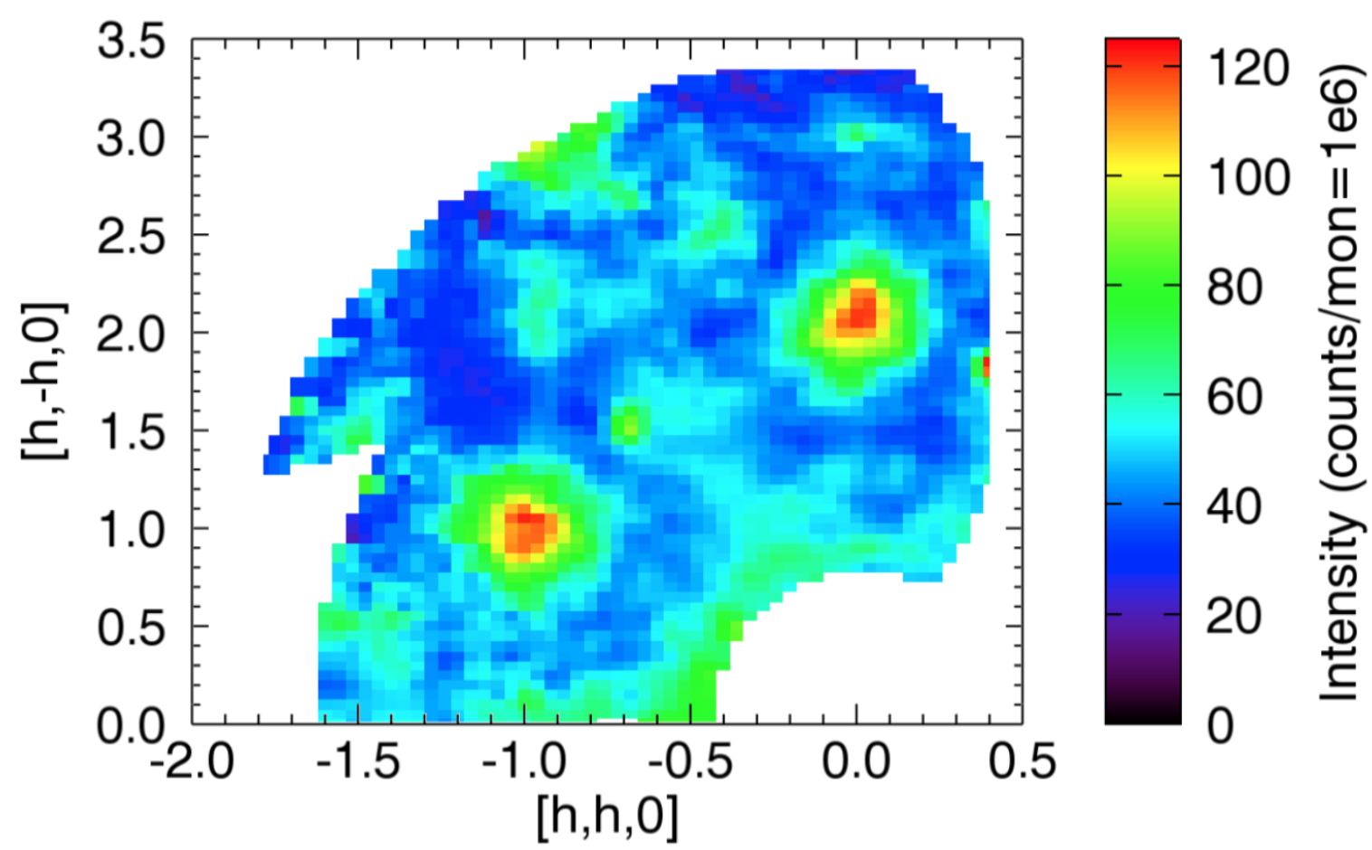
(g) INS, E = 1.4meV, T = 90mK

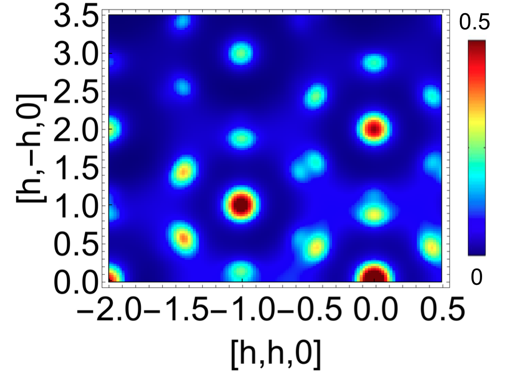
(h) $S^{\sf LSW}_{\sf T=0}({\bf q},\omega=1.4\leavevmode\nobreak\ \text{meV})$

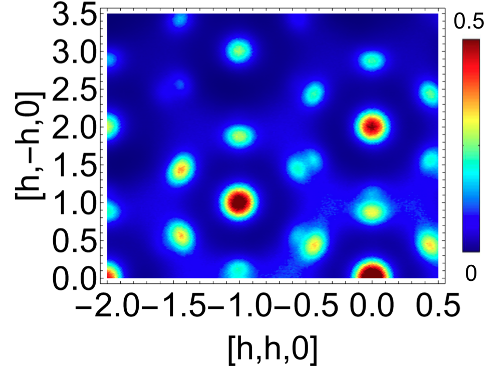
(i) $\tilde{S}^{\sf MD}_{\sf T=10mK}({\bf q},\omega=1.4\leavevmode\nobreak\ \text{meV})$

Figure 17: Spin dynamics of Ca₁₀Cr₇O₂₈ in the saturated state at $B=11$T. (a), (d), (g) Results for inelastic neutron scattering (INS) experiments, reproduced from Balz et al. (2016, 2017b), are compared to (b), (e), (h) linear spin-wave (LSW) theory and (c), (f), (i) molecular dynamics (MD) results of the bilayer breathing-kagome (BBK) model ${\cal H}_{\sf BBK}$ [Eq. (1)], with parameters taken from Tab.2. (a)–(c) Gapped, dispersing spin-wave excitations along the [h, -h, 0] direction. (d)–(f) Gapped, dispersing spin-wave excitations along the [2+h, -2 + h, 0] direction. Constant energy cut at (g) – (i) E = 1.4 meV shows bright features corresponding to high intensities in the spin-wave dispersion. In order to compare to INS data, results for LSW theory and MD simulations are presented with a Gaussian convolution of FWHM = 0.2 meV and Cr⁵⁺ form factor. INS results were taken at $T=90$mK, while LSW theory corresponds to the T = 0 quantum case. MD simulations have been performed at $T=10$mK, while presented in its temperature corrected form $\tilde{S}(\omega,{\bf q})$ [Eq. (17)], in order to compare to T = 0 LSW theory.

Meanwhile, for $0.225<B<0.375\ \text{T}$, where the heat–capacity peak splits, the maximum in $\chi^{\perp}_{\phi}(T)$ is found at the same temperature as the lower peak in $c(T)$ [Fig. 15(b)], consistent with the existence of a lattice–nematic state at low temperatures.

V.4 Competing (quasi–)ordered phases

At temperatures between the two peaks in specific heat [Fig. 15a], we find a phase that lacks $Z_{3}$ order [Fig. 15(b)], but shows spin correlations very similar to those observed in a triple–q state triangular lattice Okubo et al. (2012); a known example of a skyrmion lattice [Fig. 15(c,d)]. At higher temperatures, these give way to the known correlations of the spiral spin liquid [Fig. 15(e,f)].

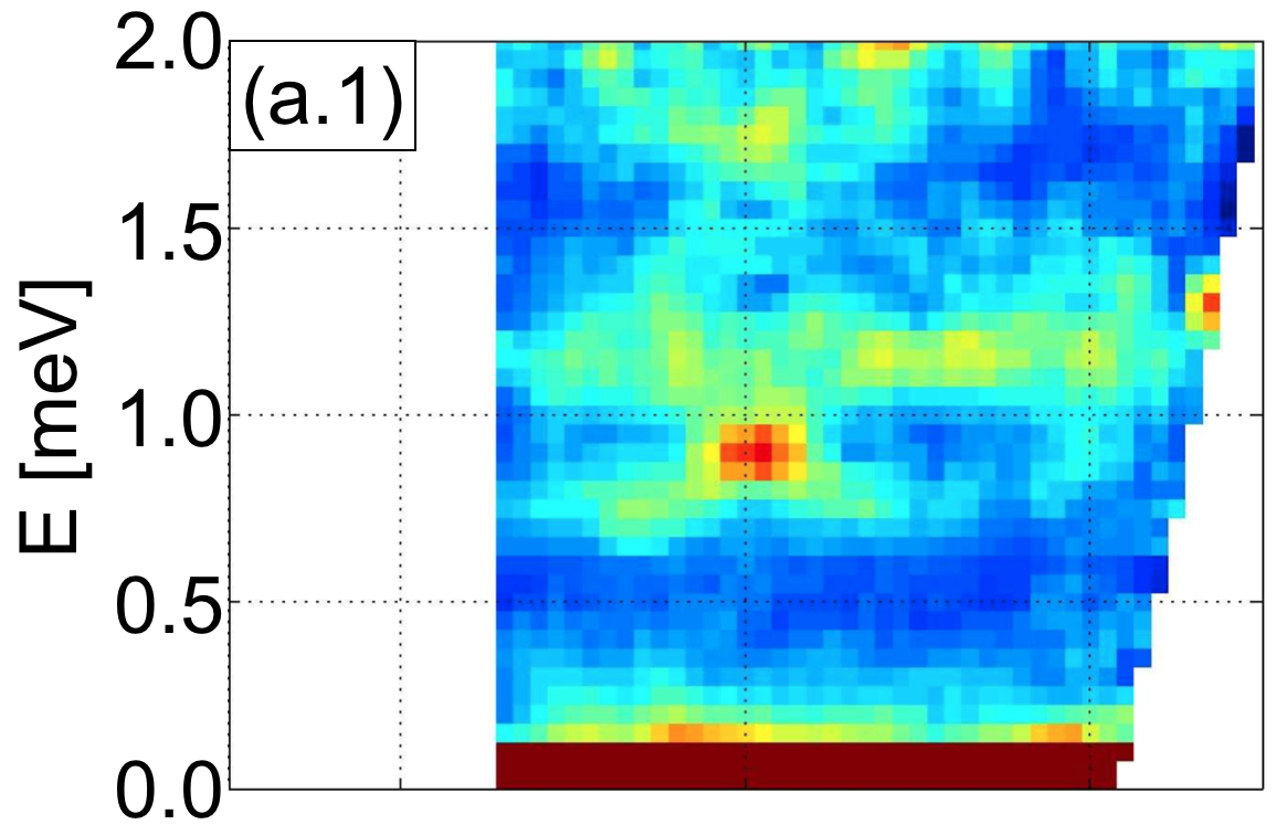
$B=7.5$T

(a)

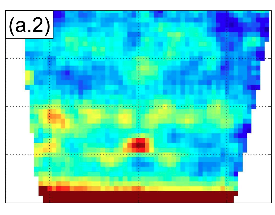
$B=5$T

(b)

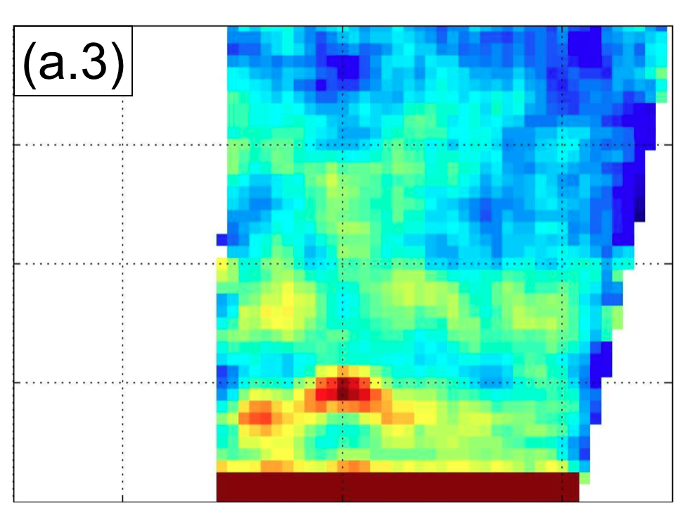
$B=4$T

(c)

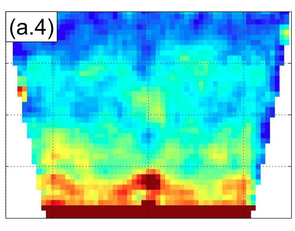
$B=3$T

(d)

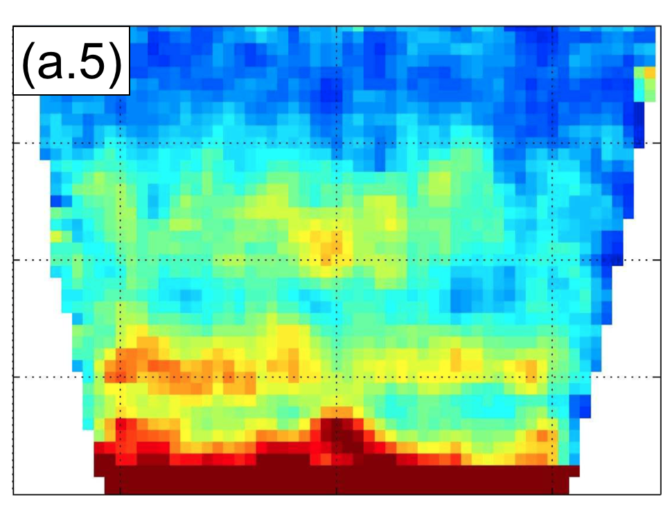
$B=2$T

(e)

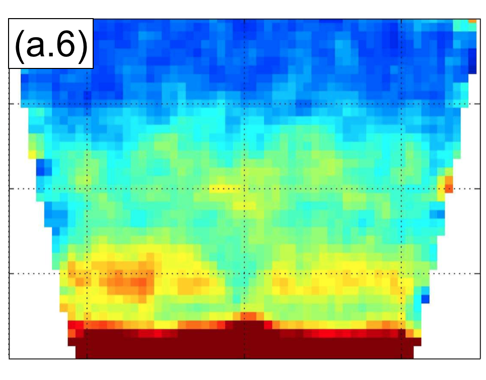
$B=1$T

(f)

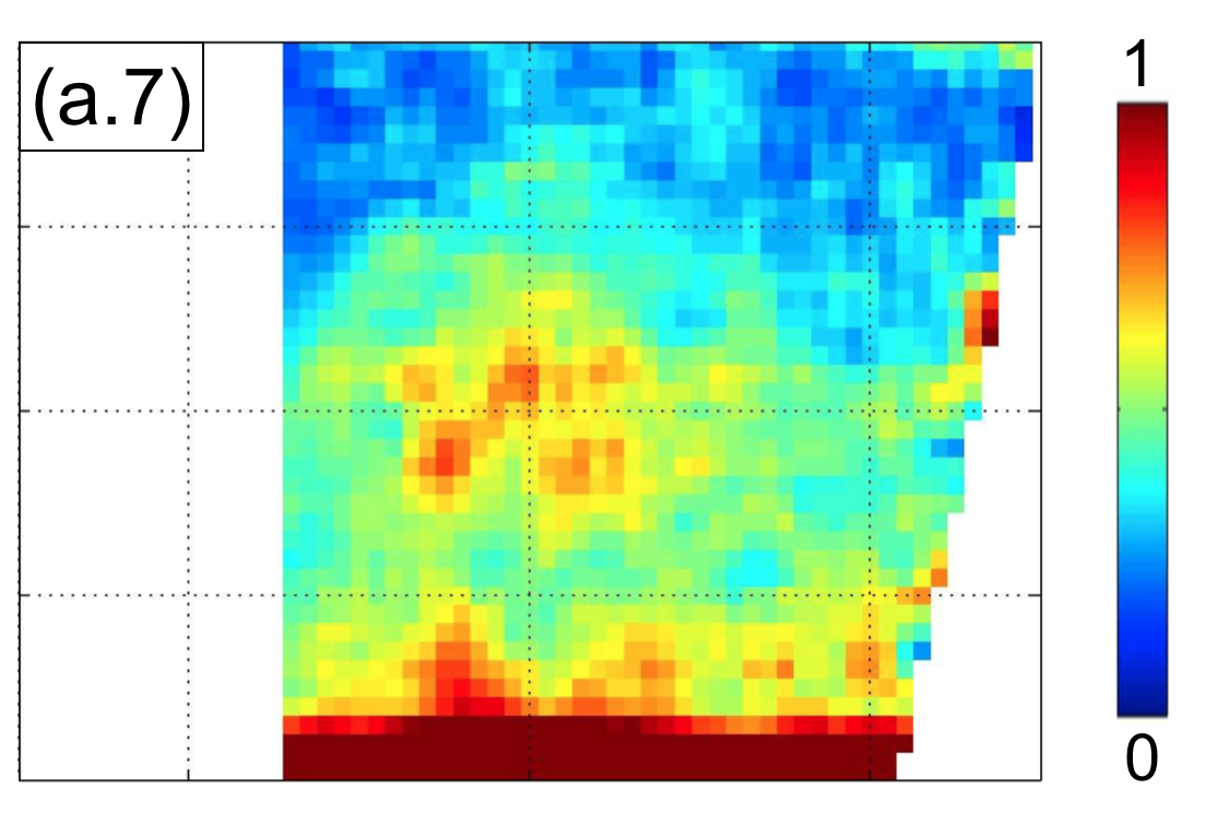
$B=0$T

(g)

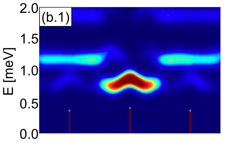
(h)

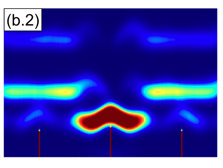
(i)

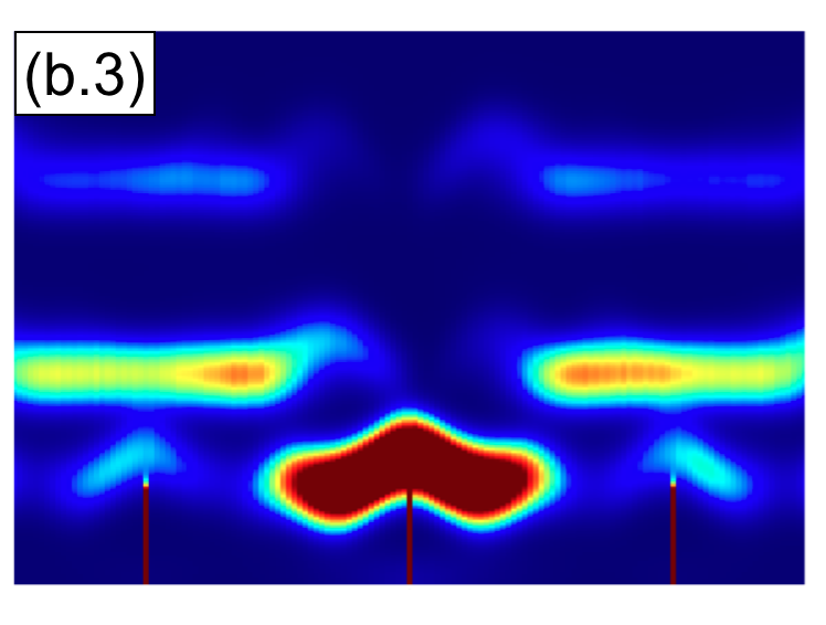
(j)

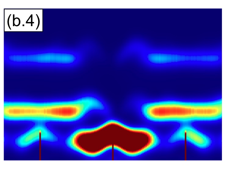
(k)

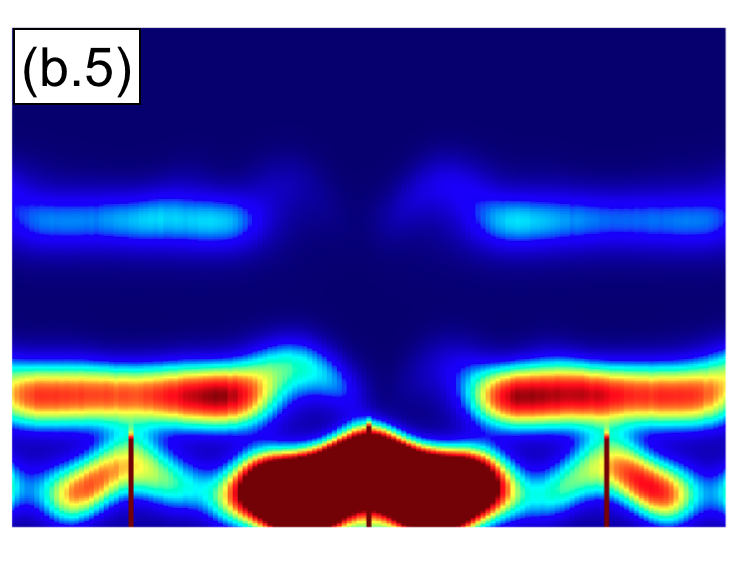
(l)

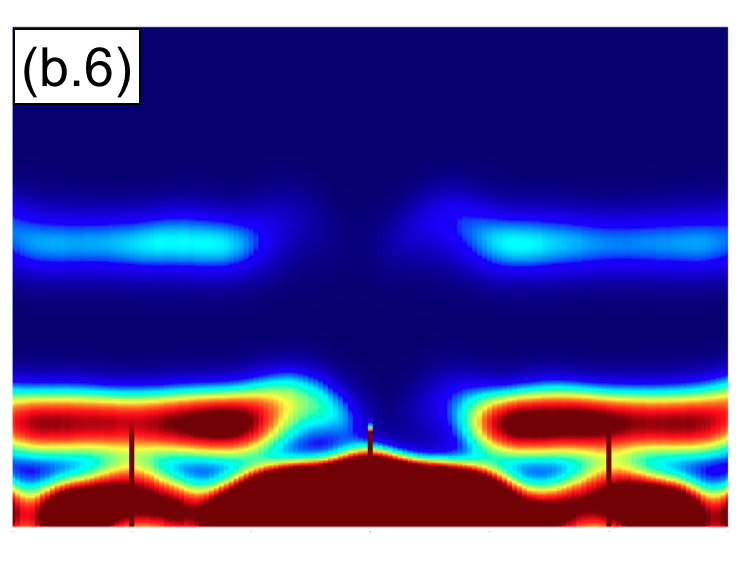
(m)

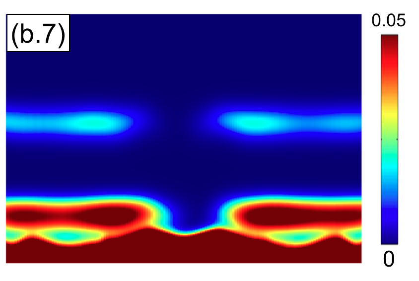
(n)

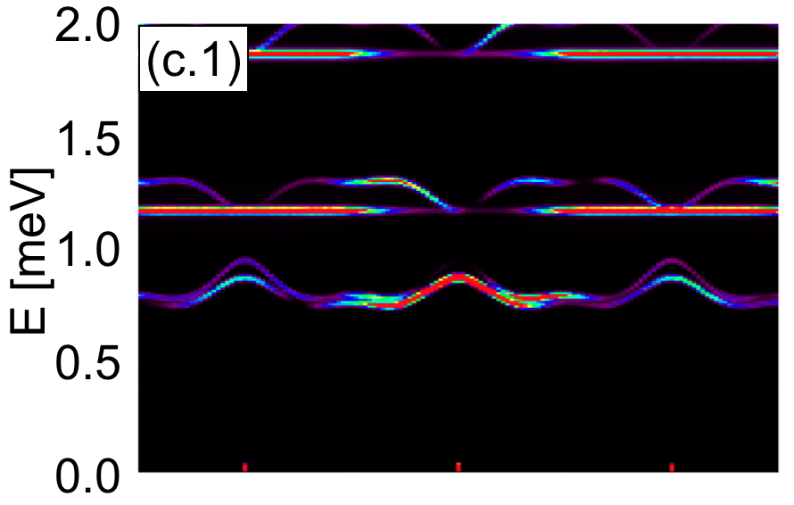
(o)

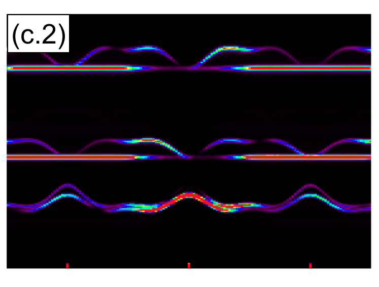
(p)

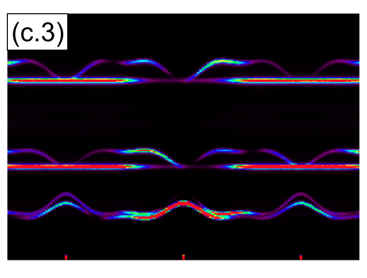
(q)

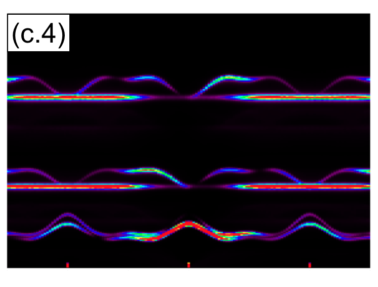
(r)

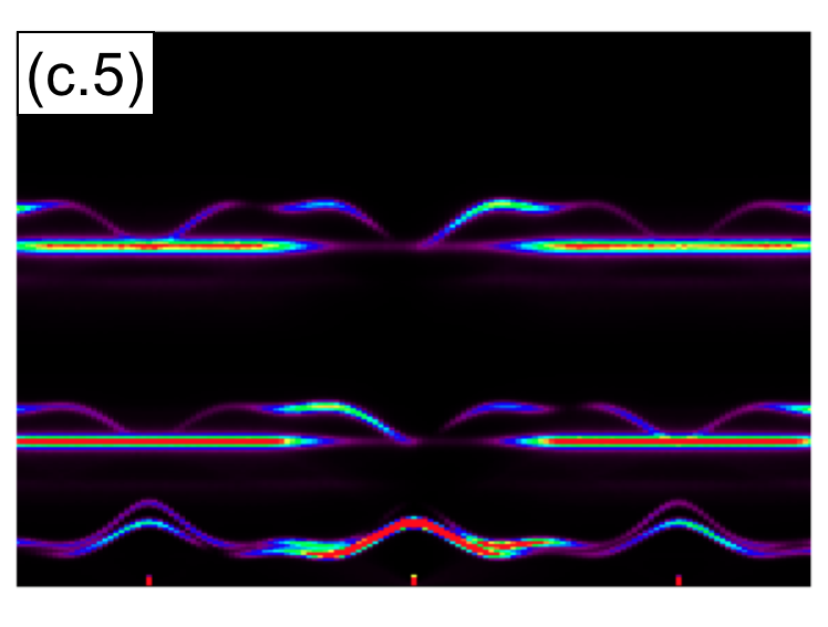
(s)

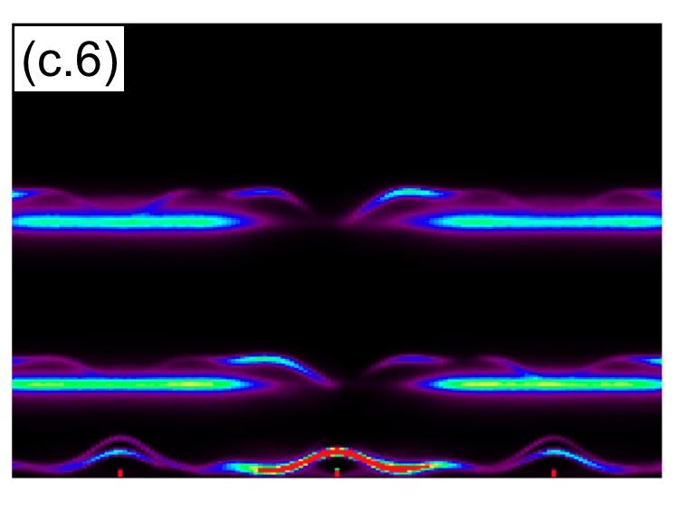
(t)

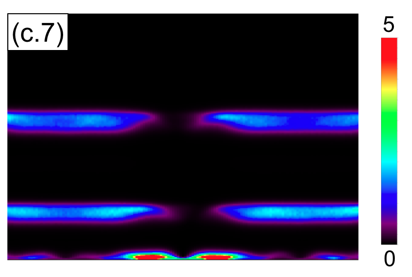
(u)

(v)

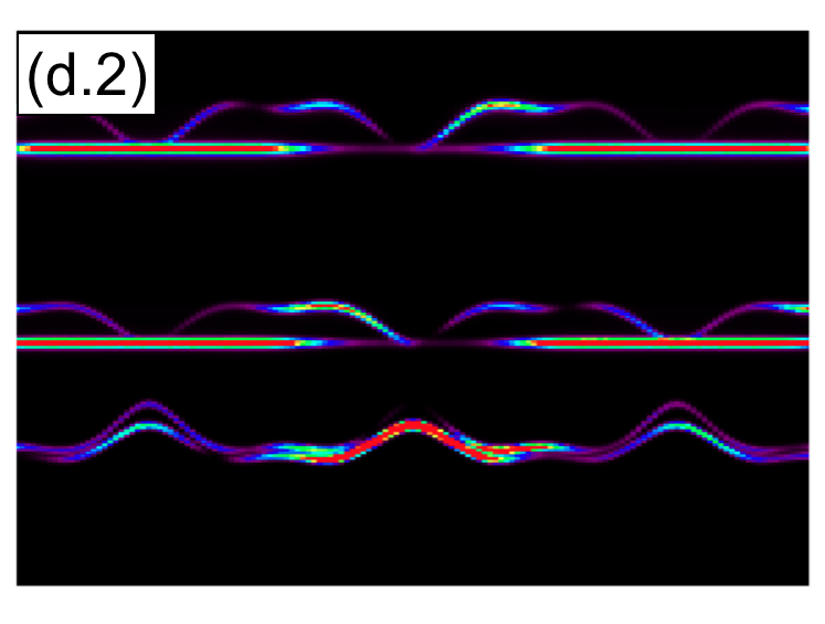
(w)

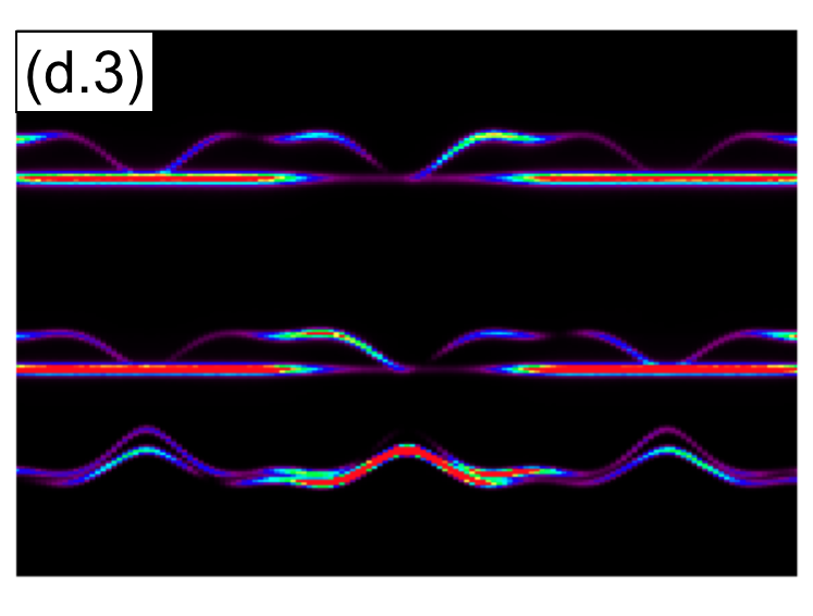
(x)

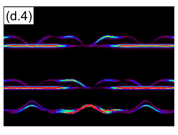
(y)

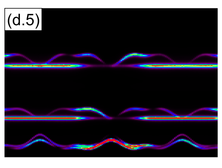
(z)

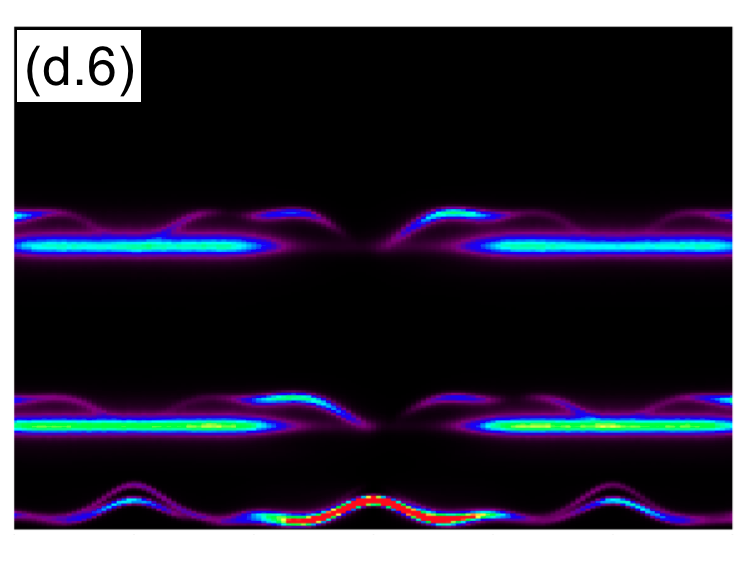
(aa)

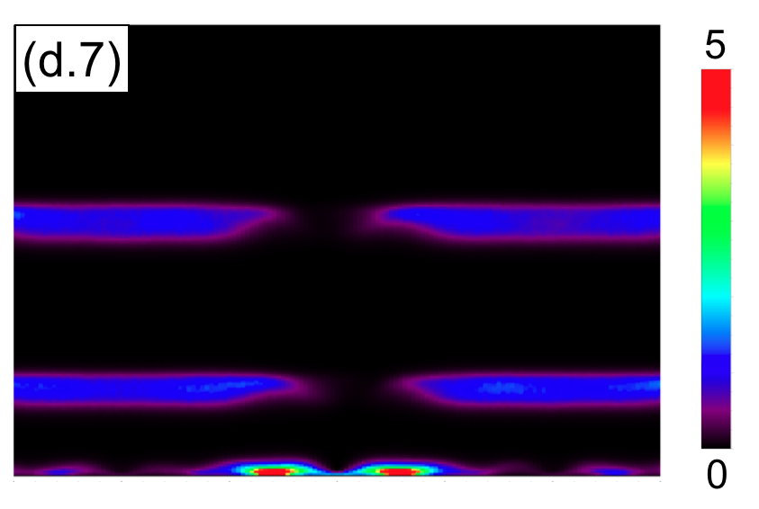
(ab)

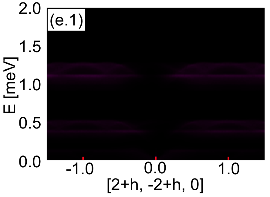
(ac)

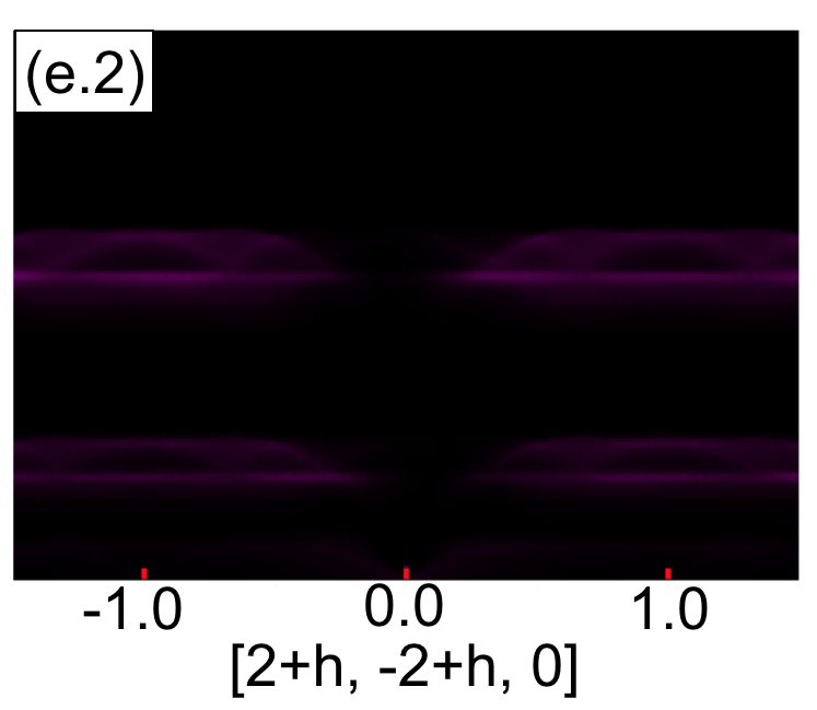
(ad)

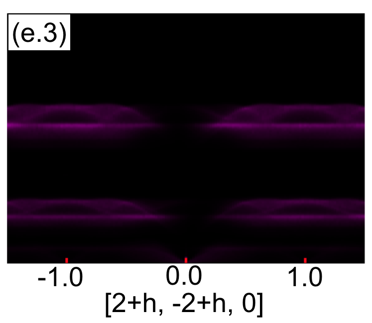
(ae)

(af)

(ag)

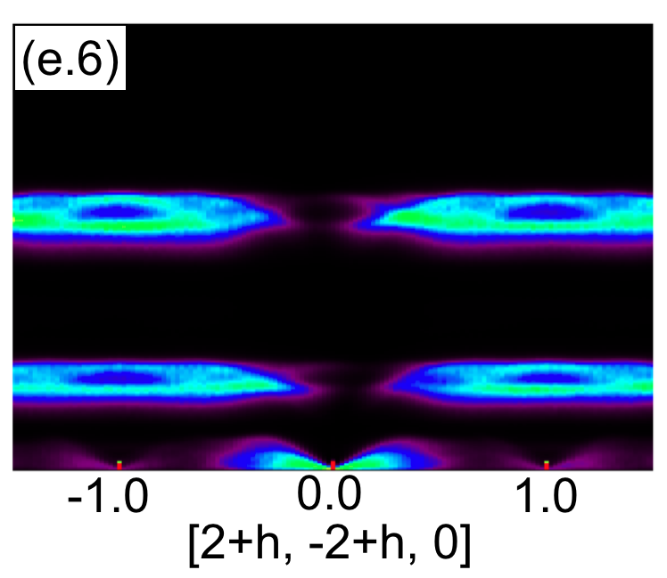
(ah)

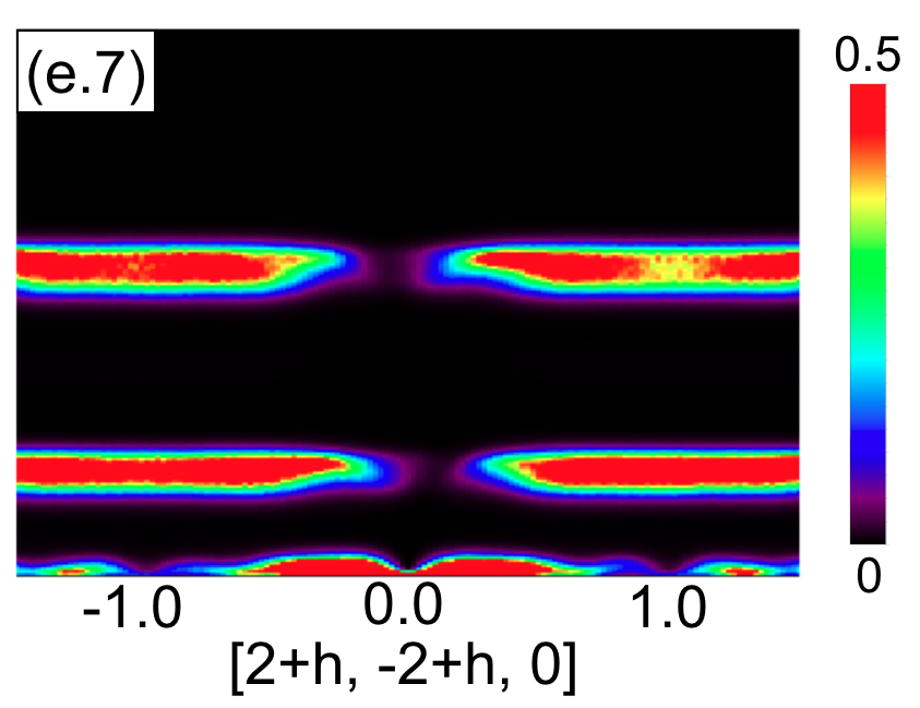
(ai)

Figure 18: Evolution of spin excitations as a function of magnetic field at $T=220$ mK, with high resolution in frequency space. (a) Inelastic neutron scattering results for Ca₁₀Cr₇O₂₈ , reproduced from Balz et al. (2017a), for magnetic fields ranging from $B=7.5\ \text{T}$ to $B=0\ \text{T}$. (b) Predictions for inelastic scattering taken from MD simulations of ${\mathcal{H}}_{\sf BBK}$, as described in the Sec. A. Results are shown along the $[2+\text{h},-2+\text{h},0]$ direction, integrated over $\pm 0.2$ r.l.u. perpendicular to the cut in reciprocal space, and convoluted with a gaussian in frequency space of FWHM $\approx$ 0.2meV, and Cr⁵⁺ form factor to compare with experiments in (a). (c) Simulation results for the first moment of the dynamical structure factor $\tilde{S}({\bf q},\omega)$ [Eq. (17)], with better energy resolution of FWHM = 0.02meV. (d) Contribution to $\tilde{S}({\bf q},\omega)$ coming from transverse spin fluctuations $\tilde{S}^{\bot}({\bf q},\omega)$ [Eq. (22)]. (e) Contribution to $\tilde{S}({\bf q},\omega)$ coming from longitudinal spin fluctuations $\tilde{S}^{\parallel}({\bf q},\omega)$ [Eq. (23)].

For higher values of magnetic field, $0.375<B\lesssim 1\ \text{T}$, there is only a single sharp feature in $c(T)$, presaged by a broad shoulder at (slightly) higher temperature [Fig. 16a]. The sharp peak is found at higher temperatures than the anomaly in the $Z_{3}$ order–parameter susceptibility [Fig. 16(b)]. For $T\to 0$, the peak tends in $c(T)$ to a field $B\sim 0.9\ \text{T}$ [Fig. 14], setting the outer limits of $Z_{3}$ order.

The weaker anomaly (shoulder), meanwhile, tracks to $B\sim 1.1\ \text{T}$, the critical field found in LSW theory at $T=0$ [Figs. 12,14]. This defines a new multiple–q (II) phase, coloured pink in Fig. 12, with correlations [Fig. 16(c,d)] which are qualitatively different from those of the lattice nematic or multiple–q (I) state found at lower field [Fig. 15]. Unfortunately, the precise nature of the phases found at low temperature for this range of fields has proved extremely difficult to determine on the basis of simulations based on a local update, and further work would be needed to definitively identify this state.

V.5 Summary of results

Putting these results together, we arrive at the phase diagram shown in Fig. 12. Anomalies found in $c(T)$ and $\chi^{\perp}_{\phi}(T)$ at low temperature are marked with triangular symbols. These are taken from simulation results for a cluster of $N=1944$ spins; some way from the thermodynamic limit, but large enough to offer representative results. The single data point at $T=220\ \text{mK}$ [square symbol] is taken from studies of dynamics, described in Section VI.

Five distinct phases are shown. The phase diagram is dominated by two phases of direct relevance to experiments on Ca₁₀Cr₇O₂₈; a correlated paramagnet in which spins on triangular plaquettes are ferromagnetically aligned [shaded green]; and the finite–field continuation of the “spiral spin liquid” studied in Section IV [shaded blue]; These phases extend up to temperatures of order $T\approx 500\ \text{mK}$, where the three spins on FM plaquettes start to fluctuate independently, and the heat capacity rolls over into a paramagnetic behaviour [Fig. 7].

We also identify three (quasi–)ordered phases at low temperatures; the finite–field continuation of the $Z_{3}$ lattice nematic studied in Section III.1 [shaded orange]; a “multiple–q (I)” state [shaded magenta]; and a “multiple–q (II)” phase [shaded pink], which have both multiple–q character. The shaded region separating the “multiple–q (II)” phase from the lattice nematic is not identified as a new phase, but indicates the splitting of anomalies in $c(T)$ and $\chi^{\perp}_{\phi}(T)$, which is subject to strong finite–size scaling.

Current results leave a number of open questions about the nature of (quasi–)ordered phases found in the classical limit of the BBK model at low temperature. However, as these do not appear to be of direct relevance to Ca₁₀Cr₇O₂₈, and are difficult to probe with current simulation techniques, we leave them for future work. Here, a good first step towards understanding these phases might be to extend simulations of the equivalent $S=3/2$ $J_{1}$–$J_{2}$ honeycomb–lattice model Biswas and Damle (2018) to finite magnetic field.

VI Dynamical properties of BBK model in field

Having explored the thermodynamics of the BBK model in field, we now turn to its dynamics, where it is possible to make explicit connection with the inelastic neutron scattering results of Balz et al. Balz et al. (2016, 2017a). We start with results for high field, where experiments were been used to parameterise the BBK model of Ca₁₀Cr₇O₂₈, before returning to the question of how a spin liquid emerges from a field–saturated state.

VI.1 Dynamics in high field

In simulation as in experiment, results are most easily understood for high magnetic fields, where the magnetization is saturated. Here, the fact that the BBK model is invariant under rotations about the magnetic field, implies that linear spin wave (LSW) theory provides an exact description of the one–magnon excitations of a fully polarised state at $T=0$. We start by exploring the properties of the six dispersing bands of spin waves in this case.

In Fig. 17 we show results for the dynamical structure factor $S({\bf q},\omega)$ in a magnetic field of $B=11\ \text{T}$, well above the saturation field $B\sim 1\ \text{T}$. For comparison we show results taken from MD simulation ($T=10\ \text{mK}$), LSW theory ($T=0$), and INS data ($T=90\ \text{mK}$). To aid comparison, both MD and LSW results for $S({\bf q},\omega)$ have been convoluted with an experimental “resolution function” (a Gaussian of FWHM $\Delta E_{\sf sim}=0.2\ \text{meV}$), and with the atomic form factor for Cr⁵⁺ [Appendix C]. In this limit, once thermal occupation factors have been corrected for [cf. Eq. (17)], the agreement between MD and LSW results is essentially perfect, establishing that MD simulation also accurately describes these excitations. Both LSW and MD results also offer a good account of the main features of experiment, confirming that the parameters found by Balz et al. Balz et al. (2016, 2017a), are a reasonable starting point for describing Ca₁₀Cr₇O₂₈.

VI.2 Evolution of dynamics with reducing magnetic field

We now turn to the question of how the relatively simple spin dynamics of the saturated state of Ca₁₀Cr₇O₂₈, evolve into the complex behaviour of the spin liquid at zero field. We take as a starting point Fig. 8 of Balz et al. (2017a), where INS results measured at $T=220\ \text{mK}$ are presented for magnetic fields in the range $0\leq B\leq 7.5\ \text{T}$. These data, for a cut through reciprocal space $[2+\text{h},-2+\text{h},0]$, are reproduced in Fig 18(a). They show a progressive evolution of the broad dispersing features found at high field [cf. Fig. 17], towards the relatively diffuse scattering of the spin liquid at $B=0\ \text{T}$, with results for $E\lesssim 0.15\ \text{meV}$ obscured by a strong incoherent elastic background.

In Fig 18(b), we present equivalent results for the dynamical structure factor of the BBK model. These are taken from MD simulations carried out at $T=220\ \text{mK}$, well above the transition temperature for the lattice–nematic or multiple–q states [Fig. 12]. To facilitate comparison with experiment, the magnetic form factor of Cr⁵⁺ has been taken into account, and results have been integrated over $\pm 0.2$ r.l.u. perpendicular to the cut in reciprocal space. They have also been convoluted with a Gaussian in frequency space of FWHM $\Delta E\approx 0.2\ \text{meV}$. Processed in this way, simulation results provide a good account of experimental data for $B\geq 1\ \text{T}$, and capture many of the key features for $B=0\ \text{T}$ [cf. Fig. 2]. However, because of the information lost in convolution, it is relatively difficult to identify the six dispersing magnon bands of the saturated state, or to disentangle the different types of fluctuation within the spin liquid for $B\leq 1\ \text{T}$.

To shed more light on these questions, in Fig 18(c), we show results at the native energy–resolution of the MD simulations, with FWHM $\Delta E=0.02\ \text{meV}$. In this case, no attempt has been made to correct for the magnetic form factor of Cr⁵⁺, experimental resolution, or the polarisation–dependence of scattering. However, in order to compensate for the classical statistics of the MC simulations, we plot the temperature–corrected dynamic structure factor $\tilde{S}({\bf q},\omega)$ [Eq. (17)]. At high values of field, we can distinguish six different branches of spin-wave excitations, in correspondence with the results of linear spin-wave theory Balz et al. (2017a). The intermediate and high–energy spin–wave branches are qualitatively similar, containing flat bands of localised spin-wave excitations, similar to those found in the Heisenberg antiferromagnet on the kagome lattice Garanin and Canals (1999); Zhitomirsky (2008); Taillefumier et al. (2014). The low–energy branches are qualitatively different, and it is the lowest of these that encodes the “ring” characteristic of the spiral spin liquid, in the form of a set of quasi–degenerate minimima close to the zone boundary.

In Fig. 18(d) and Fig. 18(e), we show equivalent results, separated into transverse

$$\tilde{S}^{\perp}({\bf q},\omega) = \frac{1}{2}\frac{\omega}{k_{B}T}S^{\perp}({\bf q},\omega)\;,$$ (22)

and longitudinal components

$$\tilde{S}^{\parallel}({\bf q},\omega) = \frac{1}{2}\frac{\omega}{k_{B}T}S^{\parallel}({\bf q},\omega)\;,$$ (23)

as defined in Appendix A [Eqs. (46)–(49)]. At high fields, $\tilde{S}_{\perp}({\bf q},\omega)$, clearly distinguishes the six branches of spin–wave excitations, while $\tilde{S}_{\parallel}({\bf q},\omega)$ shows spectral weight at $\omega\approx 0.5\ \text{meV}$ and $\omega\approx 1.2\ \text{meV}$, suggestive of bands of (highly–localised) longitudinal excitations. With reducing magnetic field, the spin–wave branches decrease in energy, at constant intensity, while longitudinal excitations remain fixed in energy, but gain in spectral weight.

At $B=1\ \text{T}$, transverse excitations show a small gap [Fig. 18(d6)], while longitudinal excitations [Fig. 18(e6)] have gained enough spectral weight for a zero–energy feature resembling a small “volcano” to be distinguished in the zone center. Finally, at $B=0\ \text{T}$, transverse [Fig. 18(d7)] and longitudinal [Fig. 18(e7)] excitations merge into the three diffuse bands documented in Fig. 11.

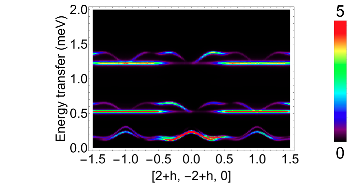
(a) $\tilde{S}^{\bot}({\bf q},\omega)$

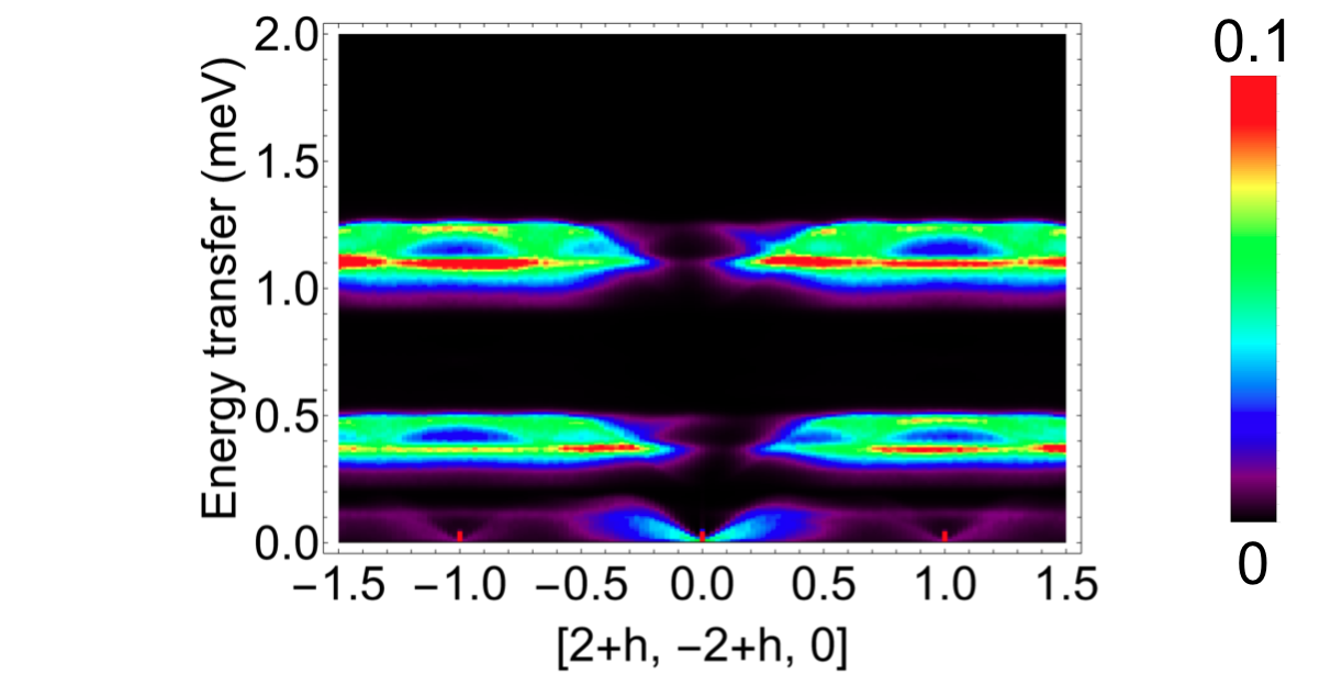
(b) $\tilde{S}^{\parallel}({\bf q},\omega)$

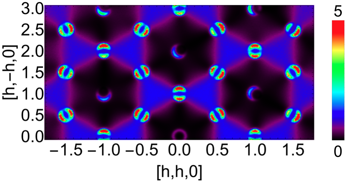
(c) $\tilde{S}^{\bot}({\bf q},\omega=0.55\text{meV})$

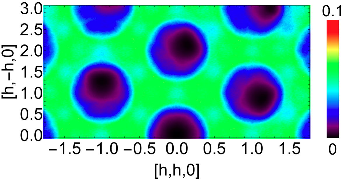
(d) $\tilde{S}^{\parallel}({\bf q},\omega=0.46\text{meV})$

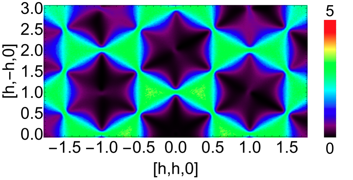
(e) $\tilde{S}^{\bot}({\bf q},\omega=0.51\text{meV})$

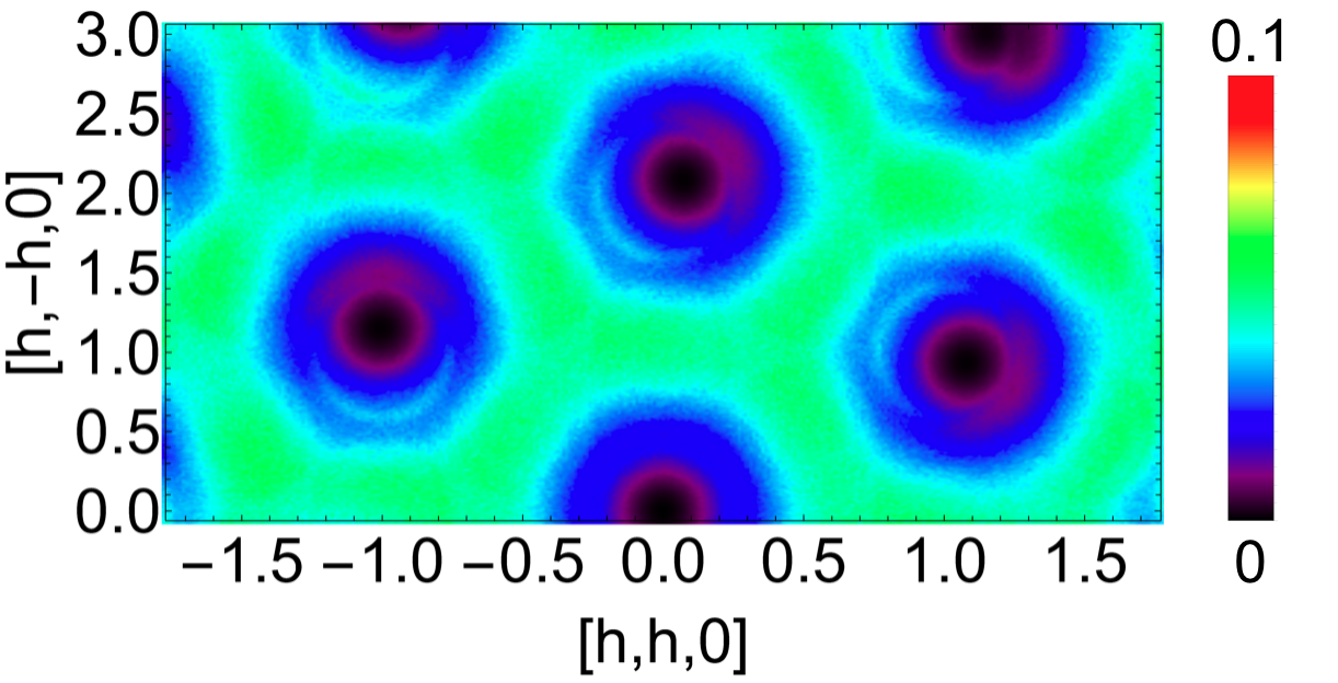
(f) $\tilde{S}^{\parallel}({\bf q},\omega=0.34\text{meV})$

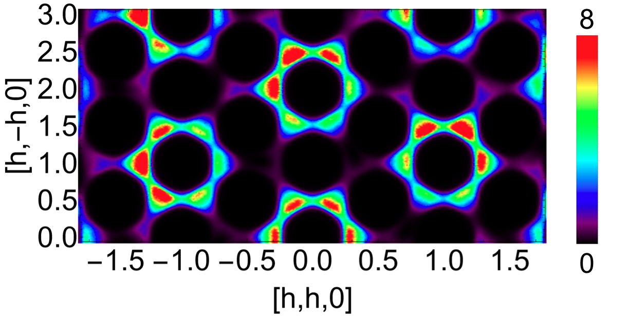
(g) $\tilde{S}^{\bot}({\bf q},\omega=0.12\text{meV})$

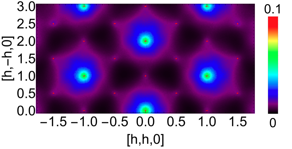
(h) $\tilde{S}^{\parallel}({\bf q},\omega=0.01\text{meV})$

Figure 19: Detail of spin dynamics at $B=2\ \text{T}$, showing the qualitatively different character of excitations in the transverse and longitudinal channels. (a) Temperature corrected transverse structure factor, $\tilde{S}^{\bot}({\bf q},\omega)$ [Eq. (22)], showing six distinct branches of spin–wave excitations. (b) Temperature corrected longitudinal structure factor, $\tilde{S}^{\parallel}({\bf q},\omega)$ [Eq. (23)], showing weakly–dispersing longitudinal spin excitations at three distinct energy scales. (c) Transverse correlations at intermediate energy, $\omega=0.55\ \text{meV}$, showing “half–moon” features overlaid on a lattice of “bow–ties” (pinch points). (d) Longitudinal correlations at $\omega=0.46\ \text{meV}$, showing a network of broad scattering. (e) Transverse correlations at $\omega=0.51\ \text{meV}$, showing sharp pinch–point features. (f) Longitudinal correlations at $\omega=0.34\ \text{meV}$, showing evolution of the network of broad scattering. (g) Transverse correlations at low energy, $\omega=0.12\ \text{meV}$, showing the ring–like feature associated with the spiral-spin liquid. (h) Longitudinal correlations at $\omega=0.01\ \text{meV}$, showing the elastic peaks associated with finite magnetisation in zone centers, and accompanying broad, diffuse scattering. All results were obtained from molecular dynamics (MD) simulation of the BBK model, Eq. (1), at $T=220\ \text{mK}$, with parameters taken from Experiment [Table 2]. System sizes are of linear dimension $L=48$ ($N=13,824$), while the energy resolution is FWHM = 0.02 meV, in absence of the Cr⁵⁺ form factor.

VI.3 Longitudinal and transverse modes at $2\ \text{T}$

In Fig. 19 we document the different types of correlation associated with transverse and longitudinal modes, at $B=2\ \text{T}$ and $T=220\ \text{mK}$. This value of field lies well within the correlated PM [Fig. 12], and the expected six bands of transverse spin–wave excitations are visible in $\tilde{S}^{\perp}({\bf q},\omega)$ [Fig. 19a]. However the magnetisation is not yet saturated [Fig. 13], and significant spectral weight can also be found in the longitudinal excitations probed by $\tilde{S}^{\parallel}({\bf q},\omega)$ [Fig. 19b]. In both cases, excitations can be divided into low–, intermediate– and high energy bands [cf. First Animation fir ], with the structure of intermediate– and high–energy correlations being broadly similar. However, while transverse excitations form sharp dispersing bands, longitudinal ones are much more diffuse in character. And, while transverse excitations show an energy gap $\Delta\approx 0.3\ \text{meV}$, longitudinal excitations are gapless.

When we examine the correlations at fixed energy, these differences become more stark. At intermediate energy, the transverse structure factor reveals characteristic “half moon” features [Fig. 19c], dispersing out of bow–tie like “pinch points” encoded on a flat band [Fig. 19e]. Both of these structures reflect the existence of a local constraint Yan et al. (2018), a point which we return to below.

Longitudinal correlations at similar energies, meanwhile, show a broad web of scattering near to the zone boundary [Fig. 19d, 19f]. And at low energies, correlations look even more different, with $\tilde{S}^{\perp}({\bf q},\omega=0.12\ \text{meV})$ showing the same “ring” of excitations near the zone boundary as the spiral spin liquid Section III [Fig. 19g], while $\tilde{S}^{\parallel}({\bf q},\omega=0.01\ \text{meV})$ is dominated by a volcano-like structure near the zone center [Fig. 19h]. Interestingly, a similar structure has been reported within the parton–phenomenology of Sonnenschein et al. Sonnenschein et al. (2019), where gapless excitations arise from low–energy particle–hole pairs spanning the Fermi surface, and is also seen in exact–diagonalization studies Shimokawa et al. (tion).

VI.4 Characterisation of pinch points and half moons

The combination of pinch–point and half–moon features observed in the spin–wave bands of the field–saturated state [Fig. 19] is a ubiquitous feature of frustrated magnets realising (or proximate to) a classical Coulombic spin liquid Robert et al. (2008); Guitteny et al. (2013); Fennell et al. (2014); Taillefumier et al. (2014); Petit et al. (2016); Rau and Gingras (2016); Udagawa et al. (2016); Benton (2016a); Mizoguchi et al. (2017); Lhotel et al. (2017); Yan et al. (2018); Mizoguchi et al. (2018), and is well–characterised in the case of the Kagome–lattice antiferromagnet Robert et al. (2008); Taillefumier et al. (2014); Yan et al. (2018). While they might at first sight appear different, pinch points and half moons have a common origin, stemming from the local constraint associated with the (proximate) spin liquid Henley (2010). In what follows, we outline how it is possible to construct a theory of these features by generalising the semi–classical analysis given in Yan et al. (2018) to the BBK lattice.

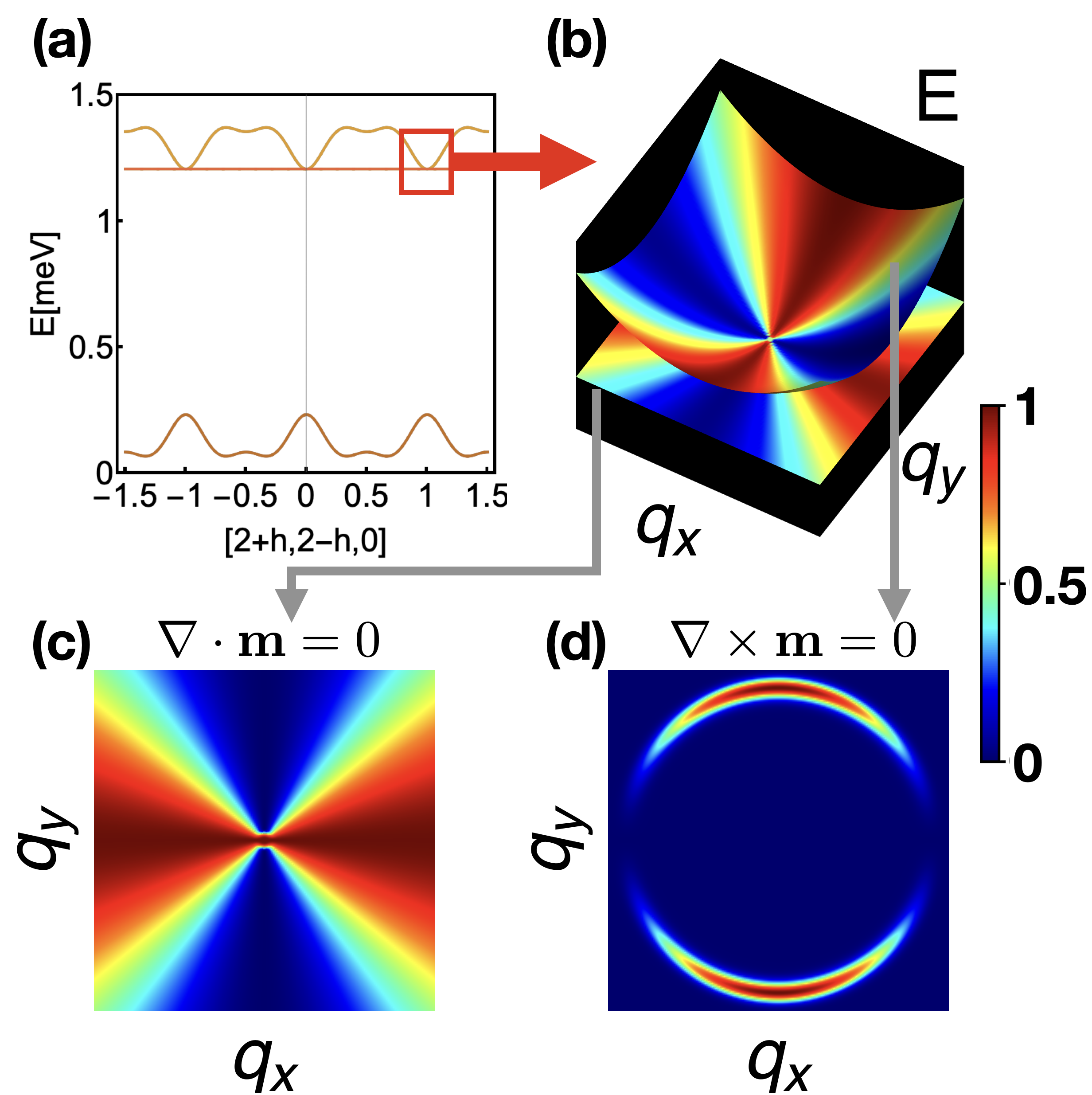
Figure 20: Schematic illustration of the pinch points and half moons coming from a single breathing–Kagome layer in applied magnetic field. (a) Spin–wave dispersion of field–saturated state. The upper pair of bands correspond to excitations satisfying either a zero–divergence or a zero–curl condition. (b) Detail of dispersion in zone center, where the upper pair of bands touch. The contribution made by each band to the equal–time structure factor $S({\bf q})$ is shown in colour. (c) Correlations at fixed energy in the flat band, showing the pinch point in the dynamical structure factor $S({\bf q},\omega)$, coming from the divergence–free condition. (d) Correlations at fixed energy in the neighbouring dispersing band, showing the pair of half moons in $S({\bf q},\omega)$, coming from the curl–free condition. Results are shown for the upper layer of the breathing bilayer Kagome (BBK) model of Ca₁₀Cr₇O₂₈ [Fig. 1, Eq. (1)], with parameters taken from experiment [Table 2], and magnetic field $B=2\ \text{T}$.

Before considering the BBK model of Ca₁₀Cr₇O₂₈, it is helpful to consider the simpler example of a Kagome lattice antiferromagnet whose magnetisation has been saturated by magnetic field, as studied in Yan et al. (2018). Here we specialise to a single breathing–Kagome (BK) layer, with parameters $J_{22}$ and $J_{31}$ taken from the BBK model of Ca₁₀Cr₇O₂₈ [Table 2]. The primitive unit cell for this BK lattice is a triangle, containing three sites, and the field–saturated state therefore supports three bands of transverse spin–wave excitations, shown in Fig. 20(a). We focus on the two upper bands of excitations, one flat, and one dispersing, which touch in zone centers [Fig. 20(b)]. What is interesting about these two magnon bands is that the eigenvectors associated with the flat band have a divergence–free character, while the eigenvectors associated with the dispersing band have a curl–free character Yan et al. (2018). And within a (semi–)classical evolution of spin configurations, these two types of excitations entirely decouple from one another Benton (2016b); Yan et al. (2018).

When it comes to evaluation of equal–time structure factors $S({\bf q})$ [Fig. 20(b)], both zero–divergence and zero–curl excitations exhibit “pinch points”, singular features resembling a “bow tie” Henley (2005). In the case of the zero–divergence excitations, these pinch points are visible in the dynamical structure factor $S({\bf q},\omega)$ when $\omega$ is tuned to the energy of the flat band [Fig. 20(c)]. Meanwhile, since the pinch points of the zero–curl excitations are inscribed on a dispersing band, they manifest as “half moons” in $S({\bf q},\omega)$ [Fig. 20(d)].

We now return to the (weakly) localised bands of excitations found at intermediate and high energies in the BBK model of Ca₁₀Cr₇O₂₈. The properties of these bands are not very different from the Kagome lattice model considered in Yan et al. (2018), with the obvious caveat that there are now two copies of each type of excitation, and so four bands in total. The fact that these “duplicate” bands are not degenerate reflects the fact that exchange interactions in the two Kagome layers of Ca₁₀Cr₇O₂₈ are not identical [Table 2], and that interlayer coupling mixes the bands associated with each layer. However, the key physics – decoupling of the curl–free and the divergence–free excitations – remains valid, and gives rise to pinch–point and half–moon features in $S({\bf q},\omega)$, [Fig. 21].

Now let us develop the mathematics of this picture. We start by constructing the long-wavelength fields that describe the transverse excitations of a polarised state, and define the vector field. We explicitly consider a single bilayer of a breathing Kagome lattice [Fig. 1], as two (breathing) Kagome lattices, for each of which the primitive unit cell is a triangle, labelling triangles in “top” and “bottom” layers of the lattice "t" and "b" respectively. We then introduce fields describing transverse spin excitations which transform with the $\mathsf{E}$ (vector) and $\mathbf{A}$ (scalar) irreps of the point group of a triangle

$${\bf m}_{\mathsf{t/b}}=\sum\limits_{i=1}^{3}S^{-}_{\mathsf{t/b,}i}{\bf u}_{i}\;,\qquad\phi_{\mathsf{t/b}}=\sum_{i=1}^{3}S^{-}_{\mathsf{t/b,}i},$$ (24)

where

$$S^{-}_{i}=S_{i}^{x}-iS_{i}^{y}$$ (25)

are spin lowering operators, and

$${\bf u}_{1}=(0,1),\ {\bf u}_{2}=(-\sqrt{3}/2,1/2),\ {\bf u}_{3}=(\sqrt{3}/2,1/2)\;,$$ (26)

are (unit) vectors pointing from the center towards the corners of each triangle. ${\bf m}_{\mathsf{t/b}}$ are the vector fields and $\phi_{\mathsf{t/b}}$ the scalar fields of interest.

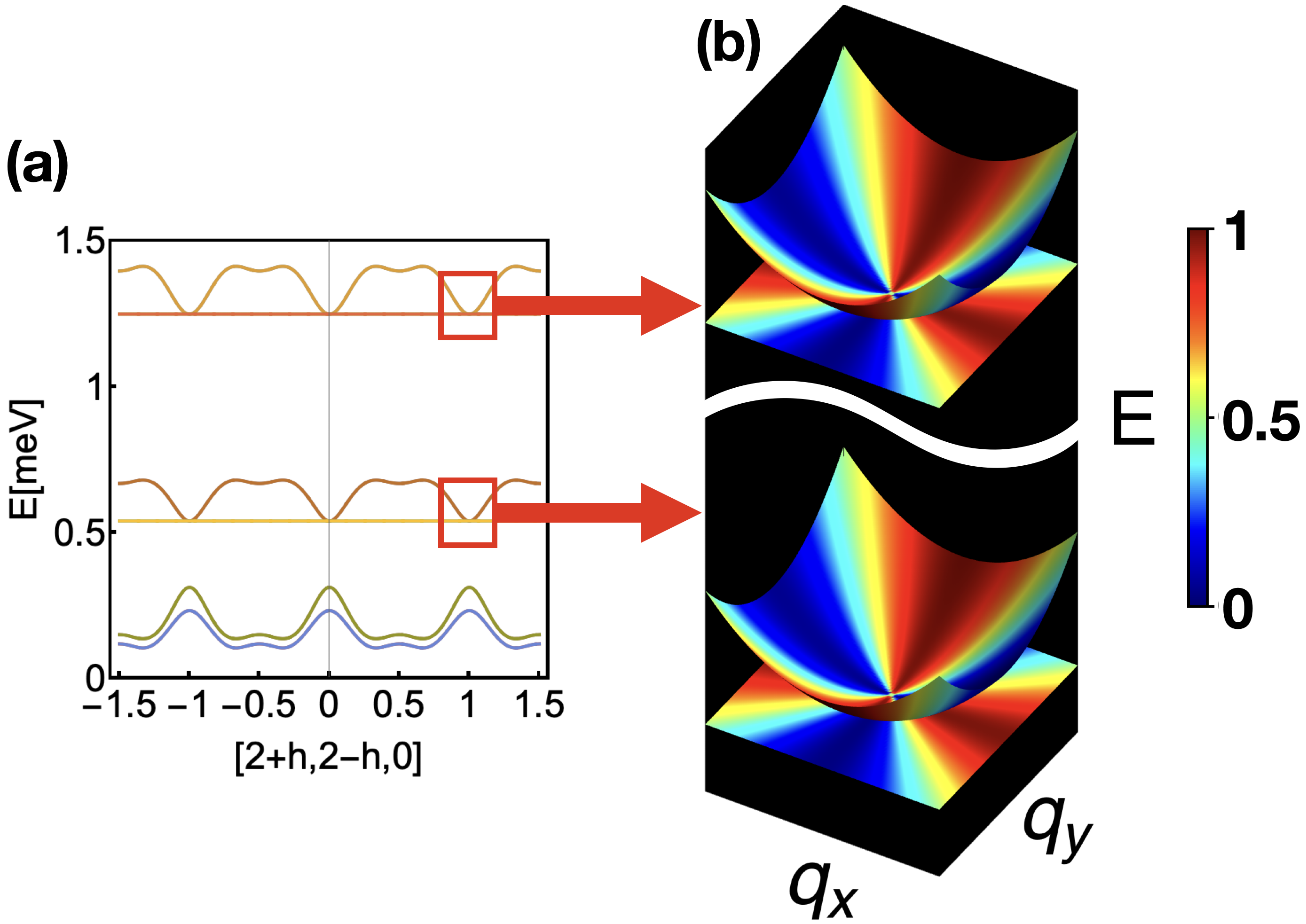
Figure 21: Schematic illustration of the relationship between flat and dispersing bands and pinch points in the bilayer—breathing Kagome (BBK) model of Ca₁₀Cr₇O₂₈. (a) Spin–wave dispersion of field–saturated state, showing pairs of bands at low, intermediate and high energy. The two dispersive bands at intermediate and high energy correspond to curl–free excitations on each layer, mixed by interlayer interactions [Eq. (35),(36)]. Meanwhile, the adjoining flat bands correspond to the divergence–free excitations on each layer, mixed by interlayer interactions [Eq. (33),(34)]. (b) Detail of the upper pairs of bands near their zone–center touching points. Pinch points are imprinted on all four bands as a consequence of the curl– and divergence–free conditions [Eq. (32),(31)]. These are visible as either pinch points or half moons in the dynamical structure factor $S({\bf q},\omega)$, as illustrated in Fig. 20. Results are shown for the BBK model Eq. (1), with parameters taken from experiment [Table 2], and magnetic field $B=2\ \text{T}$.

By evaluating the commutation relations between ${\bf m}_{\mathsf{t/b}}$ and the BBK Hamiltonian [Eq. (1)], we obtain the equations of motion (EoM) for ${\bf m}_{\mathsf{t/b}}$. Their diagonalization exhibits the dispersion relations for the bands involved, and also the corresponding eigenstates. In the long wavelength limit, they take the form

$$-i\frac{\partial}{\partial_{t}}{\bf m}_{\mathsf{t}}= -\frac{1}{4}a_{0}^{2}J_{\mathsf{t}+}{\nabla}({\nabla}\cdot{\bf m}_{\mathsf{t}})$$ (27)

$$+\left(H^{z}-3J_{\mathsf{t}+}-\frac{1}{2}J_{\text{inter}}\right){\bf m}_{\mathsf{t}}$$

$$+J_{\text{inter}}{\bf m}_{\mathsf{b}}\;,$$

$$-i\frac{\partial}{\partial_{t}}{\bf m}_{\mathsf{b}}= -\frac{1}{4}a_{0}^{2}J_{\mathsf{b}+}{\nabla}({\nabla}\cdot{\bf m}_{\mathsf{b}})$$ (28)

$$+\left(H^{z}-3J_{\mathsf{b}+}-\frac{1}{2}J_{\text{inter}}\right){\bf m}_{\mathsf{b}}$$

$$+J_{\text{inter}}{\bf m}_{\mathsf{t}}\;,$$

where we assumed a perfect bilayer Kagome lattice with lattice constant $a_{0}$ for simplicity and

$$J_{\mathsf{t}+} = \frac{1}{2}\left(J_{31}+J_{22}\right)\;,$$

$$J_{\mathsf{b}+} = \frac{1}{2}\left(J_{32}+J_{21}\right)\;,$$ (29)

$$J_{\text{inter}} = J_{0}\;.$$

We have further simplified the equations of motion by neglecting terms coupling the fields ${\bf m}_{\mathsf{t/b}}$ to the fields $\phi_{\mathsf{t/b}}$ in Eq. (27) and Eq. (28). They can be included at the cost of a more complicated description of the problem, but do not play any significant role in the long wavelength limit.

Note that the first terms on the right hand side of the EoM is curl-free. This means the EoM can be partially decoupled by introducing a Helmholtz–Hodge decomposition of the vector field

$${\bf m}_{\mathsf{t/b}}={\bf m}_{\mathsf{t/b,DF}}+{\bf m}_{\mathsf{t/b,CF}}$$ (30)

in terms of divergence–free components

$$\nabla\cdot{\bf m}_{\mathsf{t/b,DF}}=0$$ (31)

and curl–free components

$$\nabla\times{\bf m}_{\mathsf{t/b,CF}}\equiv\left(-\frac{\partial}{\partial_{y}},\frac{\partial}{\partial_{x}}\right)\cdot{\bf m}_{\mathsf{t/b,CF}}=0.$$ (32)

This leads to the decoupled EoM for divergence–free components

$$-i\frac{\partial}{\partial_{t}}{\bf m}_{\mathsf{t,DF}}= \left(H^{z}-3J_{\mathsf{t}+}-\frac{1}{2}J_{\text{inter}}\right){\bf m}_{\mathsf{t,DF}}$$ (33)

$$+J_{\text{inter}}{\bf m}_{\mathsf{b,DF}}\;,$$

$$-i\frac{\partial}{\partial_{t}}{\bf m}_{\mathsf{b,DF}}= \left(H^{z}-3J_{\mathsf{b}+}-\frac{1}{2}J_{\text{inter}}\right){\bf m}_{\mathsf{b,DF}}$$ (34)

$$+J_{\text{inter}}{\bf m}_{\mathsf{t,DF}}\;.$$

And the decoupled EoM for curl–free components are

$$-i\frac{\partial}{\partial_{t}}{\bf m}_{\mathsf{t,CF}}= -\frac{1}{4}a_{0}^{2}J_{\mathsf{t,CF}+}{\nabla}({\nabla}\cdot{\bf m}_{\mathsf{t,CF}})$$ (35)

$$+\left(H^{z}-3J_{\mathsf{t}+}-\frac{1}{2}J_{\text{inter}}\right){\bf m}_{\mathsf{t,CF}}$$

$$+J_{\text{inter}}{\bf m}_{\mathsf{b,CF}}\;,$$

$$-i\frac{\partial}{\partial_{t}}{\bf m}_{\mathsf{b,CF}}= -\frac{1}{4}a_{0}^{2}J_{\mathsf{b}+}{\nabla}({\nabla}\cdot{\bf m}_{\mathsf{b,CF}})$$ (36)

$$+\left(H^{z}-3J_{\mathsf{b}+}-\frac{1}{2}J_{\text{inter}}\right){\bf m}_{\mathsf{b,CF}}$$

$$+J_{\text{inter}}{\bf m}_{\mathsf{t,CF}}\;.$$

Let us look at the EoMs for the divergence–free components ${\bf m}_{\mathsf{b/t,DF}}$ first. We will find they are responsible for the flat bands with pinch points. The EoM for them, Eqs. (33) and (34), couple the divergence-free components between themselves, but they decouple from all the other degrees of freedom. In the absence of spatial derivatives on the right hand side of EoM, they describe a pair of flat bands, split by a gap of

$$\Delta_{\mathsf{DF}}=2\sqrt{9(J_{\mathsf{b}+}-J_{\mathsf{t}+})^{2}+4J_{\text{inter}}^{2}}\approx 0.7\ \text{meV}\;,$$ (37)

as found in MD simulation [Fig. 19a], and illustrated in Fig. 21a. Furthermore, the divergence–free condition, Eq. (31), implies that correlations of these fields show an (algebraic) singularity with the form of a “pinch point”

$$q^{\alpha}{m}_{\mathsf{DF}}^{\alpha}=0\rightarrow\langle{m}_{\mathsf{DF}}^{\alpha}({\bf q}){m}_{\mathsf{DF}}^{\beta}({\bf-q})\rangle\sim\delta^{\alpha\beta}-\frac{q^{\alpha}q^{\beta}}{{\bf q}^{2}}\;.$$ (38)

This leads to a corresponding singularity in the dynamical spin structure factor

$$S^{\perp}_{\lambda}({\bf q},\omega) \propto (1-{q^{\lambda}_{\alpha}q^{\lambda}_{\beta}}/{{\bf q}^{2}})\delta(\omega-\omega^{\lambda}({\bf q}))\;,$$ (39)

where $\omega^{\lambda}({\bf q})$ is a constant energy of the associated (flat) band. This is the origin of the bow–tie like pinch point feature seen in MD simulation results [compare Fig. 19e with Fig. 20c ].

Very similar considerations apply to the EoM for curl–free components of ${\bf m}$, Eqs. (35), (36). They are responsible for the dispersive bands with pinch points [Fig. 21b]. In zone centers, the two bands derived from these EoM are degenerate with the two flat bands derived from divergence–free components of ${\bf m}$. However the presence of a term with spatial derivative, ${\nabla}({\nabla}\cdot{\bf m}_{\mathsf{CF}})$, leads to non-flat dispersion of the bands. The gap between the flat and dispersive band opens quadratically in zone centers [Fig. 19a and Fig. 21a].

The curl–free condition is also encoded in the correlation function as a pinch point, but this time rotated by $\pi/2$ with respect to those of the divergence–free bands

$$\langle{m}_{\mathsf{CF}}^{\alpha}({\bf q}){m}_{\mathsf{CF}}^{\beta}({\bf-q})\rangle\sim\delta^{\alpha\beta}-\frac{\tilde{q}^{i}\tilde{q}^{j}}{{\bf q}^{2}}\quad{\bf\tilde{p}}=(-p_{y},p_{x})$$ (40)

Once again, the associated singularity is imprinted on the dynamical spin structure factor

$$S^{\perp}_{\lambda}({\bf q},\omega) \propto (1-\frac{\tilde{q}^{i}\tilde{q}^{j}}{{\bf q}^{2}})\delta(\omega-\omega^{\lambda}({\bf q}))\;,$$ (41)

where $\omega^{\lambda}({\bf q})$ is the energy of the associated (dispersing) bands. However, because the bands associated with zero–curl states have a finite dispersion, this singularity appears not as a pinch–point but as a pair of half moons in cross-sections at constant energy [compare Fig. 19c with Fig. 20d].

Comparing quantitative results for the BBK model [Fig. 21] with those for a single BK layer [Fig. 20], we see that interlayer coupling has relatively little effect on bands carrying pinch points and half moons. This reflects the fact that the interlayer coupling $J_{0}\approx-0.08\ \text{meV}$ is small compared with the splitting of the bands $\Delta_{\mathsf{DF}}\approx 0.7\ \text{meV}$ [Eq. (37)]. This should be contrasted with the situation at low energies, where interlayer coupling plays a crucial role in determining the effective honeycomb lattice model, Eq. (6), and thereby the spiral spin liquid ground state.

To summarise, the four bands of transverse spin excitations found in MD simulation of the BBK model at intermediate and high energy [cf. Section VI.1, VI.2, VI.3] can be understood as two sets of flat bands, satisfying a zero–divergence condition, and two sets of (weakly) dispersing bands, satisfying a zero–curl condition. Each of these bands support specific features in dynamical structure factors — pinch points and half moons — which are characteristic of the corresponding local constraint. Elsewhere, equivalent features at finite energy have been characterised as a “dynamical spin liquid” Petit et al. (2016); Benton (2016b); Lhotel et al. (2018). And it is a special feature of the BBK model of Ca₁₀Cr₇O₂₈ that the dynamical spin liquid found at intermediate and higher energies ultimately coexists with a completely different from of the spin liquid at low energy. It is the way in which this spiral spin liquid emerges as the ground state, as magnetic field is reduced, that we turn to below.

VI.5 Closing of gap to transverse excitations

Since the correlations of the spiral spin liquid [Fig. 6c] are encoded in the lowest lying transverse spin excitations of the high–field paramagnet [Fig. 19g], we can identify the onset of the spin liquid, with the closing of the gap to these excitations. In Fig. 22 we show the gap $\Delta(B)$ to the lowest lying excitations in $S^{\perp}({\bf q},\omega)$ evolves as a function of magnetic field, as found in MD simulations carried out at $T=220\ \text{mK}$. At higher values of field, where the magnetisation is (approximately) saturated, $\Delta(B)$ tracks the results of linear spin wave theory at $T=0$ [red line in Fig. 22(a)], which would extrapolate to the gap closing at $B=1.0\ \text{T}$. However for fields $B\lesssim 2\ \text{T}$, $\Delta(B)$ starts to deviate from the spin wave prediction [inset to Fig. 22(a)], finally closing for $B\gtrapprox 0.7\ \text{T}$. In Fig. 22(b) and (c), we show results for $S^{\perp}({\bf q},\omega)$ at $B=0.5\ \text{T}$, just below, and at $B=1.0\ \text{T}$, a little above, the closing of the gap. The corresponding estimates of the field at which the gap closes, form the basis of the phase boundary between correlated paramagnet and spiral spin liquid shown in Fig. 12.

VI.6 Summary of results for dynamics in field

In summary, the dynamics of the BBK model of Ca₁₀Cr₇O₂₈ in field reveals a number of interesting features. Firstly, dynamics in longitudinal and transverse channels are very different, with transverse dynamics showing a gap at high fields, while longitudinal dynamics remain gapless at all fields [Fig. 18].

Secondly, the lowest–lying transverse spin excitations in high field show the same “ring”–like (quasi–)degeneracy as the classical spin liquid in zero field [cf Fig. 11b with Fig. 19g]. We therefore associate the closing of the gap to these excitations, at a value of magnetic field which depends on temperature with the onset of the low–field spin–liquid state [Fig. 22].

Thirdly, transverse dynamics at high field also reveal flat bands at intermediate energy, which carry pinch–point correlations, resembling the “bow–tie” patterns observed in the spin liquid [Fig. 19e]. These are accompanied by half–moon motifs, inscribed on a dispersing band which intersects the flat band at zone centers [Fig. 19c].

We return to each of these features where we discuss the implication for experiments on Ca₁₀Cr₇O₂₈, below.

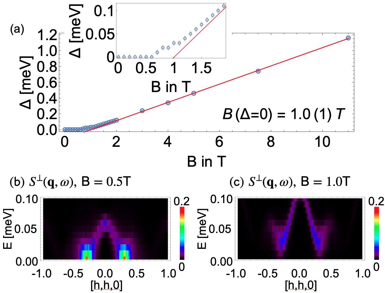
(a)

Figure 22: Evolution of gap $\Delta$ to low–lying transverse spin excitations in applied magnetic field. (a) Results for $\Delta(B)$, as found in molecular dynamics (MD) simulation at $T=220\ \text{mK}$ [cf. Fig. 18]. Red line: linear behaviour found for spin–wave excitations about the field–saturated state at $T=0$. Inset: Detail of $\Delta$ for $B\leq 2T$. (b) Detail of MD results for transverse structure factor $S_{\perp}({\bf q},\omega)$ [Eq. (21)] at $B=0.5\ \text{T}$, showing gapless spin excitations. (c) Equivalent results for $B=1.0\ \text{T}$, showing gap to transverse spin excitations. Simulations were carried out for a cluster of linear dimension L = 48 (N = 13,824), using the BBK model Eq. (1), with parameters taken from experiment [Table 2]. Error bars in (a) and pixel size in (b), (c) represent the finite-energy resolution of MD simulations, $\delta E=0.01\ \text{meV}$.

VII Application to $\text{Ca}_{10}\text{Cr}_{7}\text{O}_{28}$

In Section II.8 we identified four open questions about the BBK model of Ca₁₀Cr₇O₂₈. We now return to these, addressing each in turn, before discussing some of the features of Ca₁₀Cr₇O₂₈which still remain to be understood.

The first challenge was to connect the finite–energy and finite–temperature properties of Ca₁₀Cr₇O₂₈ with the spin–1/2 BBK model, Eq. (1). When it comes to finite–temperature properties, in the absence of magnetic field, our main results are summarised in the phase diagram, Fig. 6(a), and the associated predictions for the equal–time structure factor, Fig. 6(c,d) and Fig. 10. We find that experimental parameters [Table 2], place Ca₁₀Cr₇O₂₈ within a “spiral spin liquid” regime. This is characterised by ring–like correlations in $S({\bf q})$, and occurs for temperatures ranging from a lattice–nematic ordering transition at $T\approx 70\ \text{mK}$, to a crossover into a high–temperature paramagnet, occurring for $T\sim 500-1000\ \text{mK}$. This is consistent with experiment, where a spin liquid, characterised by ring–like structures in $S({\bf q})$, occurs in the same range of temperatures Balz et al. (2016, 2017a). And the low–temperature lattice–nematic [Section III.1], while not observed in Ca₁₀Cr₇O₂₈, is consistent with earlier simulations of an effective honeycomb lattice model Biswas and Damle (2018). Moreover, our conclusions about spin liquids at finite temperature prove to be robust for a wide range of parameters, and so are relatively insensitive to the uncertainty in estimates of exchange coupling taken from experiment Balz et al. (2016, 2017a).

Molecular Dynamics (MD) simulations give further insight into the nature of this spin liquid, through its finite–energy properties. Results for the dynamical structure factor $S({\bf q},\omega)$ are summarised in Fig. 11, in the comparison with experiment, Fig. 2, and in the two animations fir ; sec . A key feature is the separation of dynamics into three distinct time–scales; a long timescale associated with the slow, collective excitations of groups of three spins on ferromagnetically–correlated plaquettes, and intermediate and short timescales associated with qualitatively different excitations. Correlations at low energies echo the spin–liquid, with ring–like features in $S({\bf q},\omega)$, while dynamics at higher energies show a diffuse web of scattering, with bow–tie like features visible in a subset of zone centers. Ring and bow–tie features would usually be associated with qualitatively different spin–liquid states, and in this sense the BBK model appears to support different spin liquids, on different timescales, at the same time.

Experiment on Ca₁₀Cr₇O₂₈ also shows qualitatively different correlations on different time scales, with hints of rings at low energy, and bow–tie like features at intermediate and high energies Balz et al. (2016, 2017a). Where experiment and (classical) simulation differ is in the extent to which higher–energy excitations form a continuum, with MD results showing weakly–dispersing excitations at relatively well–defined energies.

The second challenge was to extend the analysis of the BBK model to finite values of magnetic field. Here, key results are summarised in the phase diagrams Fig. 3 and Fig. 12, and the associated predictions for spin dynamics, Fig. 17, Fig. 18 and Fig. 19. We find that spin–liquid correlations persist up to a temperature–dependent field $B\sim 1\ \text{T}$, but with dramatically different correlations at different energy scales, and in the transverse and longitudinal channels. At higher fields, classical simulations find a highly–correlated paramagnet, in which transverse spin excitations are gapped, but longitudinal excitations remain gapless. Meanwhile, at low temperatures, the lattice nematic gives way to a series of complex forms of order.

Once again, the phenomenology of the BBK model in field has many similarities with experiments on Ca₁₀Cr₇O₂₈. Fits to the spin wave excitations of the saturated paramagnet have already been documented Balz et al. (2016, 2017a). And the zero–field magnetic susceptibility of Ca₁₀Cr₇O₂₈ Balz et al. (2017a); Kshetrimayum et al. (2020), is also very similar to that found in the BBK model at low temperatures, with the caveat that the classical statistics of our MC simulations lead to a much stronger temperature dependence than is seen in experiment [Fig. 13]. Measurements of Ca₁₀Cr₇O₂₈ at low temperatures also exhibit a qualitative change in behaviour of $C/T$ at $B\sim 1\ \text{T}$ Balz et al. (2017a), consistent with the opening of a gap found in MD simulations. No sign has yet been seen, however, of the complex competing orders found in classical MC simulations at the lowest temperatures.

The third challenge was to identify the mechanism driving the low temperature spin liquid state. Here simulations of the BBK model offer a number of new insights. Firstly, they show a clear separation of dynamics within the spin liquid, between slow collective rotations of FM polarised triangular plaquettes, and fast excitations of individual spins [Second Animation sec ]. This confirms the validity of modelling the low–energy dynamics of Ca₁₀Cr₇O₂₈ in terms of spin–3/2 moments on a honeycomb lattice, a construction which has played an important role in existing classical Biswas and Damle (2018) and quantum Sonnenschein et al. (2019) theories of Ca₁₀Cr₇O₂₈. Secondly, the correlations found at low energy are consistent with a spiral spin liquid, while those at higher energies resemble those of a Kagome anitferromagnet [Fig. 2, Fig. 11]. And thirdly, the onset of spiral spin liquid behaviour can be identified with the closing of the gap to transverse excitations at $B\sim 1\ \text{T}$ [Fig. 22]. A key feature of this transition is the (quasi–)degeneracy of the “ring” of excitations at the bottom of the spin–wave spectrum, all of which participate in the resulting spin liquid. While the equivalent quantum theory remains an open problem, this scenario has much in common with the formation of a chiral spin liquid through the condensation of hard–core bosons in a system with a continuous, “moat”–like degeneracy Sedrakyan et al. (2015).

The fourth challenge was to identify interesting properties of the BBK model which may, as yet, be obscure in experimental data for Ca₁₀Cr₇O₂₈. Here, MD simulations reveal a number of features of the dynamics of the BBK model which it would be rewarding to look for in experiment. In particular, they suggest that the application of a magnetic field could offer new insights into the spin liquid, by separating longitudinal and transverse dynamics with dramatically different character [Fig. 18, Fig. 19]. This is something which could be probed using polarised neutron scattering. Our results also suggest that Ca₁₀Cr₇O₂₈ is a suitable system for investigating the physics of pinch points and half moons Yan et al. (2018), which play a prominent role in the excitations at finite energy. These could most easily be studied in the high–field, saturated paramagnetic state, cf. Fig. 19c.

Taken together, these results represent significant progress in understanding Ca₁₀Cr₇O₂₈. None the less, there are a number of features in experiment which remain to be understood. One is the presence of spectral weight at finite energies for wave vector ${\bf q}=0$ in the absence of magnetic field Balz et al. (2017a), something which is forbidden for a spin–rotationally invariant model like ${\cal H}_{\sf BBK}$ [Eq. (1)]. A likely explanation is the presence of anisotropic exchange interactions, including Dzyaloshinskii–Moriya (DM) terms. These are allowed by the symmetry of the lattice, and would endow the magnon bands of the field–saturated state with a topological character Romhányi . They would also contribute to the finite lifetime of excitations Chernyshev and Zhitomirsky (2015), which could help to explain their relatively broad character in experiment Balz et al. (2017a).

Another area where further investigation is merited, is the question of how the thermodynamics and spin dynamics of the BBK model of Ca₁₀Cr₇O₂₈ change once quantum statistics, and entanglement, are taken into account. Exact diagonalisation (ED), and thermal pure quantum state (TPQ) studies of the BBK model, will form the subject of a second Article Shimokawa et al. (tion). However we can already make some comparison with published results from other quantum approaches Balz et al. (2016); Kshetrimayum et al. (2020); Sonnenschein et al. (2019), which suggest that the role of quantum and thermal fluctuations in this problem may not be very different.

The biggest difference appear to arise in the zero–field ground state, where PFFRG calculations finds static correlations (characteristic “ring” in $S({\bf q},\omega=0)$) consistent with a spin liquid Balz et al. (2016). Meanwhile, tensor–network calculations report a vanishing average magnetic moment per site, coupled to a finite magnetic susceptibility, also consistent with a QSL Kshetrimayum et al. (2020). In contrast, our MC simulations show a concentration of weight in $S({\bf q})$ at the discrete set of wave vectors associated with a lattice–nematic state [Section III] and, by their nature, always exhibit a finite moment on each site. However, the ordered states found in simulation only occur at very low temperatures. And given that the model is two–dimensional, and spin excitations are (quasi–)degenerate on line–like loci, its is highly likely that quantum fluctuations would eliminate the ordered moments at the level of individual sites at zero temperature, cf. Smerald and Shannon (2010), just as thermal fluctuations do at higher temperatures. Whether the $Z_{3}$ symmetry–breaking would survive in the absence of an ordered moment is a separate, and interesting, question Mulder et al. (2010).

Even at a classical level, there are intriguing similarities in the thermodynamics, with tensor–network calculations of magnetization suggestive of phase transitions at $B\approx 0.3\ \text{T}$, $B\approx 0.8\ \text{T}$ and $B\approx 1.0\ \text{T}$ Kshetrimayum et al. (2020), scales similar to the transitions between different ordered states found in MC simulation at low temperature [Section V]. And when it comes to dynamics, it is encouraging to note the extent to which MD simulations reproduce features seen in the spinon phenomenology of Sonnenschein et al. Sonnenschein et al. (2019). In particular the “volcano” feature observed in the structure factor associated with longitudinal fluctuations $S_{\parallel}({\bf q},\omega)$ [Section VI] is very reminiscent of the low–energy cone of particle–hole excitations about the Fermi surface.

Needless to say, (semi–)classical simulations, by themselves, cannot be used to argue for the existence of spinons in Ca₁₀Cr₇O₂₈. A method with access to quantum entanglement is required Shimokawa et al. (tion). However, the congurence of experiment, simulation of the BBK model, and parton approaches does suggest that, phenomenologically, a spinon picture may not be so wide of the mark. And, as a general comment on the present state of theory of Ca₁₀Cr₇O₂₈, it is interesting to note that the picture advanced by Sonnenschein et al. Sonnenschein et al. (2019) is essentially that of a heavy Fermion superconductor Hewson (1993); Sólyom (2008); Fulde (2012), but with spinons, rather than electrons, as heavy quasi–particles.

In both heavy Fermion superconductors, and the parton phenomenology of Sonnenschein et al. Sonnenschein et al. (2019), low–energy properties are dictated by the existence of a Fermi–surface, with heavy quasiparticles that become unstable against pairing at low temperatures. An immediate implication is that the specific heat coefficent $\gamma$, and magnetic susceptibility $\chi$ are strongly enhanced, as observed in Ca₁₀Cr₇O₂₈ [Table 1]. However an important difference between the parton theory, and conventional (heavy) Fermi liquids, is that long range interactions between neutral spinons are not screened in the same way as interactions between electrons. In (2+1)D this inexorably drives $U(1)$ QSL towards a strong–coupling fixed point Lee (1989); Lee and Nagaosa (1992); Polchinski (1994); Nayak and Wilczek (1994); Altshuler et al. (1994); Kim et al. (1994); Senthil et al. (2004); Motrunich (2005), as exemplified by the $Z_{2}$ QSL ground state conjectured by Sonnenschien et al. Sonnenschein et al. (2019). And it follows that, if Ca₁₀Cr₇O₂₈ really does have (emergent) heavy Fermi quasiparticles, these should show signs of strong correlation.

A common cross–check on the degree of correlation within a heavy Fermion system is to calculate the Wilson ratio $R_{W}$, a dimensionless number formed from the (para)magnetic susceptibility $\chi_{0}$, and the linear coefficient of specific heat, $\gamma$ Sólyom (2008); Fulde (2012). By construction the Wilson ratio of a free electron gas $R_{W}=1$, while for highly—correlated electron bands, it takes on higher values. Substituting experimental parameters for Ca₁₀Cr₇O₂₈ [Table 1], we find

$$R_{W}=\frac{\pi^{2}}{\mu_{0}}\frac{\chi_{0}}{\mu_{\text{eff}}^{2}}\frac{k_{B}^{2}}{\gamma}\approx 16.2\;,$$ (42)

where details of the estimate are given in Appendix D. This value is substantially greater than the $R_{W}\approx 4$ observed for the heavy Fermion system CeCu₆ Ott (1987); Amato et al. (1987), and would place Ca₁₀Cr₇O₂₈ in a strongly–interacting Fermi–liquid regime.

We conclude the spinon phenomonlology of Ca₁₀Cr₇O₂₈  Sonnenschein et al. (2019) remains an interesting conjecture, that does not suffer from any obvious contradiction with experiment, and is therefore worthy of further investigation. And in this context it could be interesting to investigate other properties usually controlled by the Fermi surface in metals, such as (thermal) transport, and NMR $1/T_{1}$ relaxation rates. All of this, however, lies outside the scope of the present article.

VIII Conclusions

Ca₁₀Cr₇O₂₈ is a remarkable magnet, in which spin-1/2 Cr⁵⁺ ions form a bilayer breathing-kagome (BBK) lattice with complex, competing exchange interactions Balz et al. (2017b). A combination of heat-capacity, magnetization, $\mu$SR, neutron-scattering, and AC susceptibility experiments reveal Ca₁₀Cr₇O₂₈ to be a gapless quantum spin liquid (QSL), showing no sign of magnetic order down to $19\ \text{mK}$ Balz et al. (2016, 2017a). This spin liquid is charcaterised by spin fluctuations which show qualitatively different character on different timescales.

To better understand the nature and origin of the spin liquid in Ca₁₀Cr₇O₂₈, we have carried out large-scale semi-classical molecular-dynamics (MD) simulations of the minimal model of Ca₁₀Cr₇O₂₈, a Heisenberg model on the BBK lattice, with parameters taken from experiment Balz et al. (2016, 2017a). These simulations reveal a state where spins continue to fluctuate at very low temperatures, but the character of these fluctuations depends strongly on the timescale on which the dynamics are resolved, as shown in the Animations fir ; sec . This persists up to a (temperature–dependent) critical field $B_{c}\sim 1\ \text{T}$ [Fig. 12], for temperatures ranging from an ordering temperature $T\sim 70\ \text{mK}$, to a crossover into a high–temperature paramagnet for $T\sim 500\ \text{mK}$ [Fig. 3].

Within this state, we identify fluctuations at low energies with a “spiral spin liquid”, characterised by a ring of scattering in ${\bf q}$-space, and formed when the gap to a (quasi-)degenerate set of excitations closes at $B\lesssim 1\ \text{T}$ [cf. Fig. 22]. This spiral spin liquid can be described by an effective spin-3/2 Heisenberg model on a honeycomb lattice, formed by three spin-1/2 moments on the triangular plaquettes of the BBK lattice in Ca₁₀Cr₇O₂₈ [cf. Fig. 1, Fig. 4]. The FM correlations of spins within these plaquettes are evident in the collective motion resolved at low energy in MD simulation (cf. Second Animation sec ).

Meanwhile, fluctuations at higher energy inherit their character from the kagome-lattice antiferromagnet, and for $B\gtrsim 1\ \text{T}$, are characterised by sharp pinch–points in scattering Fig. 19e. These pinch points are encoded in spin fluctuations perpendicular to the applied magnetic field and can be resolved in MD simulations as collective rotations of antiferromagnetically correlated spins on shorter timescales (cf. Second Animation sec ). In the limit $B\to 0\ \text{T}$, pinch points ultimately merge with excitations in the longitudinal channel to give rise to the broader “bow–tie” features observed in inelastic neutron scattering at higher energy [cf. Fig. 2].

These simulations capture many of the features of Ca₁₀Cr₇O₂₈; correctly reproducing the value of the critical field, $B\lesssim 1\ \text{T}$ Balz et al. (2016, 2017a); providing insight into the different structures seen in inelastic neutron scattering Balz et al. (2016, 2017a); and resolving the origin of the ring features found in Pseudo-Fermion Functional Renormalisation group (PFFRG) calculations Balz et al. (2016). To the best of our knowledge, they also provide the first theoretical example of a system which behaves like different types of spin liquid on different timescales.

Given this disparity of behaviour, it is tempting to ask just how many spin liquids there are in Ca₁₀Cr₇O₂₈? Since a quantum system should have one, unique, ground state, at low temperature the answer to this question must, ultimately, be: “one”. None the less, the success of semi–classical simulations in describing experiment suggests that this one ground state must incorporate two different types of correlations; one described by effective spin-3/2 moments on a honeycomb lattice; and one corresponding to antiferromagnetic fluctuations of individual spin-1/2 moments on a bilayer breathing-kagome lattice. Unraveling the properties of this single, massively-entangled QSL, represents an exciting challenge for theory and experiment alike. And in a second paper, we will return to this in the context of quantum simulations of the BBK model of Ca₁₀Cr₇O₂₈  Shimokawa et al. (tion).

Appendix A Numerical Methods

A.1 Classical Monte Carlo

All of the results presented in this Article are based on spin configurations drawn from classical Monte Carlo simulations of ${\cal H}_{\text{\sf BBK}}$ [Eq. (1)]. Monte Carlo simulations were performed by using a local heat–bath algorithm Olive et al. (1986); Miyatake et al. (1986), in combination with parallel tempering Swendsen and Wang (1986); Earl and Deem (2005), and over–relaxation techniques Creutz (1987). Here, we chose the heat-bath algorithm, which automatically adjusts the solid angle for updated spins at their given temperatures. In this way this method is rejection free, and therefore outperforming the conventional single-spin flip Metropolis algorithm Metropolis et al. (1953) at very low-temperatures.

Within simulations, a single MC step consists of $N$ local heat–bath updates on randomly chosen sites, and two over–relaxation steps, each comprising a $\pi$–rotation of all the spins in the lattice about their local exchange fields. Simulations were performed in parallel for replicas at a range of different temperatures, with replica–exchange initiated by the parallel tempering algorithm every $10^{2}$ MC steps. Results for thermodynamic quantities were averaged over $10^{6}$ statistically independent samples, after initial $10^{6}$ MC steps for simulated annealing and $10^{6}$ MC steps for thermalisation.

A.2 Semi-Classical Molecular Dynamics

To interpret the INS data for Ca₁₀Cr₇O₂₈ Balz et al. (2016, 2017a), we rely on Molecular Dynamics (MD) simulations. These are based on the numerical integration of the Heisenberg equations of motion

$$\frac{d{\bf S}_{i}}{dt}=\frac{\mathrm{i}}{\hbar}\big{[}{\cal H}_{\sf BBK},{\bf S}_{i}\big{]}=\bigg{(}\sum_{j}J_{ij}{\bf S}_{j}-B^{z}\hat{\mathbf{z}}\bigg{)}\times{\bf S}_{i}\;,$$ (43)

where $j$ accounts for all nearest–neighbouring sites of $i$ and $J_{ij}$ is given in Table 2.

Spin configurations for MD simulation were taken from the thermal ensemble generated by classical MC simulations of ${\cal H}_{\sf BBK}$ at $T=220\ \text{mK}$, for parameters taken from experiment [cf. Table 2]. Numerical integration of Eq. (43) was then carried out using a 4^th order Runge-Kutta algorithm, as described in Press et al. (2007); Hairer et al. (1993). Simulations were performed for $N_{t}=600$ time steps, with a time–increment $\delta t$ of

$$\delta t=\frac{t_{\text{max}}}{N_{t}}=\frac{2\pi}{\omega_{\text{max}}}$$ (44)

setting a maximaum resolvable frequency of $\omega_{\text{max}}=6\ \text{meV}$.

The dynamical structure factor

$$S({\bf q},\omega)=\frac{1}{\sqrt{N_{t}}N}\sum_{i,j}^{N}\mathrm{e}^{\mathrm{i}{\bf q}({\bf r}_{i}-{\bf r}_{j})}\sum_{n}^{N_{t}}\mathrm{e}^{\mathrm{i}\omega\ n\delta t}\>\langle{\bf S}_{i}(0)\cdot{\bf S}_{j}(t)\rangle\;,$$ (45)

was calculated using Fast Fourier Transform (FFT) Frigo and Johnson (2005), and averaged over spin dynamics obtained from $500$ independent initial spin configurations. Where simulations were carried out in applied magnetic field, this was resolved in to contributions coming from transverse and longitudinal fluctuations, i.e.

$$S({\bf q},\omega)=S^{\bot}({\bf q},\omega)+S^{\parallel}({\bf q},\omega)$$ (46)

where

$$S^{\bot}({\bf q},\omega) = \frac{1}{\sqrt{N_{t}}}\sum_{n}^{N_{t}}\mathrm{e}^{\mathrm{i}\omega\ n\delta t}\>\langle{\bf S}^{\bot}_{\bf q}(t)\cdot{\bf S}^{\bot}_{\bf-q}(0)\rangle\;,$$ (47)

$${\bf S}^{\bot}_{i} = (S^{x}_{i},S^{y}_{i})\;,$$ (48)

and

$$S^{\parallel}({\bf q},\omega) = \frac{1}{\sqrt{N_{t}}}\sum_{n}^{N_{t}}\mathrm{e}^{\mathrm{i}\omega\ n\delta t}\>\langle S^{z}_{\bf q}(t)\cdot S^{z}_{\bf-q}(0)\rangle\;.$$ (49)

To avoid numerical artifacts (Gibbs phenomenon Arfken and Weber (1995)), coming from discontinuities of the finite time-window at $t=0$ and $t=t_{\text{max}}$, the time sequence of spin configurations has been multiplied by a Gaussian envelop prior to Fourier transform, imposing a maximally possible Gaussian energy resolution of FWHM = 0.02 meV, on the numerically-obtained $S({\bf q},\omega)$.

A.3 Correcting for classical statistics

The MD simulations described above inherit the classical statistics of the classical MC simulations from which spin configurations are drawn. At low temperatures, where spins are treated as classical $O(3)$ vectors, it is possible to decompose the excitations about a given ground state into $2N$ individual harmonic modes. (This approach can also be generalised to the ensemble of ground states found in classical spin liquids Shannon et al. (2010)). Each of these modes functions like a (classical) harmonic oscillator, with amplitude

$$\langle x^{2}\rangle\sim\frac{T}{\omega}$$ (50)

and at low temperatures, the spin excitations found in classical MC simulation follows this distribution of amplitudes.

MD simulations evolve spin configurations in time according to the Heisenberg equation of motion [Eq. (43)], with eigenenergies equivalent to those found in linear spin wave (LSW) approximation. However, while the harmonic excitations of a LSW theory are quantised as Bosons, with amplitude determined by a Bose factor, MD simulations inherit the classical statistics of MC simulations which, at low temperatures, are described by Eq. (50). It follows that MD simulations function in a “mixed ensemble”, with classical statistics, but semi-classical dynamics. And to obtain a valid prediction for semi–classical dynamics in the limit $T\to 0$, that can be compared directly with LSW theory at $T=0$, it is therefore necessary to “divide out” the classical statistical factor, Eq. (50).

A careful analysis of the dynamical structure factor $S_{\sf MD}({\bf q},\omega)$ found in MD simulation of a spin–1/2 moment, taking into account the mixed ensemble, leads to the result quoted as Eq. (17) of main text

$$\tilde{S}({\bf q},\omega)=\frac{1}{2}\frac{\omega}{k_{B}T}S_{\sf MD}({\bf q},\omega)\;,$$ (51)

where $\tilde{S}({\bf q},\omega)$ is the corresponding prediction for quantum (semi–classical) dynamics in the limit $T\to 0$. Details of this calculation will be reported elsewhere Remund et al. .

Appendix B Real-time animation

Here we provide technical details of the animations of MD simulation results discussed in Section IV.2 and Section IV.4. Both animations were prepared using the open-source software package “Blender” ble .

B.1 First Animation

In the First Animation fir , we show a “fly through” of spins on the breathing bilayer-kagome (BBK) lattice, for a cluster of $N=5400$ sites, at a temperature of $T=220\text{mK}$. The total number of time steps in the simulation was $N_{t}=6000$, and in order to obtain a smooth rotation of spins in the animation, the time step for each frame has been set to $\delta t\approx 0.1\ \hbar\text{meV}^{-1}$ [cf. Eq.(44)], which is of the order of a femto second. To emphasize the dynamics on different timescales, spins have been color-coded according to their speed of rotation, with red indicating fast rotation, and green denoting slow rotation.

B.2 Second Animation

In the Second Animation sec we show results taken from a single MD simulation of ${\mathcal{H}}_{\sf BBK}$, equivalent to that shown in the First Animation. However in this case, the time sequence for the spin dynamics has been separated into slow, intermediate and fast components, to emphasise the dynamics on different timescales. This is accomplished by first performing a fast Fourier transform (FFT) on the time sequence of each spin, then filtering the resulting signal in frequency space, using a digital analogue of a “band-pass” filter. The frequencies used for this band-pass filter are equivalent to energies of $0.750$–$1.500\ \text{meV}$ (fast fluctuations); $0.225$–$0.750\ \text{meV}$ (intermediate fluctuations); and $0.00$–$0.225\ \text{meV}$ (slow fluctuations). After filtering in frequency, a second FFT is used to reconstruct separate time sequences for slow, intermediate and fast fluctuations. The final result for each of these is presented in the three panels of the Second Animation.

In the second part of the Second Animation, the speed of playback for three time sequences has been adjusted, so as to match the characteristic speed of the relevant fluctuations. To accommodate this, a much longer sequence of $N_{t}=130000$ time steps has been generated from MD simulation, using a much shorter time increment of $\delta t\approx 0.035\ \hbar^{-1}\text{meV}^{-1}$. The adjustment of playback speed has been accomplished within “Blender” ble , by adjusting the number of frames included for each time sequence. Viewed in this way, the very different dynamics on different timescales is self-evident.

Appendix C Comparison with Experiment

Predictions for inelastic neutron scattering are plotted as

$$\frac{d^{2}\sigma}{d\Omega dE_{f}} \propto I({\bf q},\omega)$$ (52)

where we calculate

$$I({\bf q},\omega) = \mathcal{F}({\bf q})^{2}\sum_{\alpha,\beta}\bigg{(}\delta_{\alpha\beta}-\frac{q_{\alpha}q_{\beta}}{{\bf q}^{2}}\bigg{)}S^{\alpha\beta}({\bf q},\omega)\;.$$ (53)

Here $\mathcal{F}({\bf q})$ is the atomic form factor appropriate to a Cr⁵⁺ ion, and following Dianoux and Lander , we write

$$\mathcal{F}({\bf q})=\langle j_{0}({\bf q})\rangle+\bigg{(}1-\frac{2}{g}\bigg{)}\langle j_{2}({\bf q})\rangle\;.$$ (54)

We consider gyromagnetic ratio $g=2$, implying that $\langle j_{2}({\bf q})\rangle$ plays no role. The remaining function, $\langle j_{0}({\bf q})\rangle$ can be parameterised as

$$\langle j_{0}({\bf q})\rangle=Ae^{-a(|{\bf q}|/4\pi)^{2}}+Be^{-b(|{\bf q}|/4\pi)^{2}}+Ce^{-c(|{\bf q}|/4\pi)^{2}}+D\;,$$ (55)

where, be consistent with earlier work Balz , coefficients are taken to be

$$A =-0.2602\;,\ B=0.33655\;,\ C=0.90596\;,\ D=0.0159$$ (56)

$$a =0.03958\;,\ b=15.24915\;,\ c=3.2568\;.$$ (57)

For comparison with experiment, following [Balz et al., 2016] and [Balz et al., 2017a], MD results for $S({\bf q},\omega)$ have further been convoluted in energy with a Gaussian of FWHM = 0.2 meV.

Appendix D Estimate of Wilson Ratio

The Wilson ratio is a dimensionless ratio of the (para)magnetic susceptibility of a metal, $\chi_{0}$, to the linear coefficient of its specific heat, $\gamma$, with parameters chosen such that the ratio takes on the value one in a free electron gas. It is defined to be Sólyom (2008); Fulde (2012)

$$R_{W}=\frac{\pi^{2}}{\mu_{0}}\frac{\chi_{0}}{\mu_{\text{eff}}^{2}}\frac{k_{B}^{2}}{\gamma}\;,$$ (58)

where the effective magnetic moment

$$\mu_{\text{eff}}=\sqrt{j(j+1)}g\mu_{B}\;.$$ (59)

For comparison with experiment on Ca₁₀Cr₇O₂₈, we take

$$j=1/2\ \;\text{and}\;g=2\;.$$ (60)

The remaining parameters, in cgs units, are given by

$$k_{B} =1.381\times 10^{-16}\ \frac{\text{erg}}{\text{K}}\;,$$ (61)

$$\mu_{B} =9.274\times 10^{-21}\ \frac{\text{erg}}{\text{G}}\;,$$ (62)

$$\mu_{0} =1\ \frac{\text{G}}{\text{Oe}}\;.$$ (63)

Taking values of $\chi_{0}$ and $\gamma$ from experiment [Table 1],

$$\chi_{0}=3\ \frac{\text{emu}}{\text{mol Oe }}=3\ \frac{\text{erg}}{\text{mol Oe G}}\;,$$ (64)

and

$$\gamma=1.35\times 10^{4}\ \frac{\text{mJ}}{\text{mol }\text{K}^{2}}=1.35\times 10^{8}\ \frac{\text{erg}}{\text{mol }\text{K}^{2}}\;,$$ (65)

we obtain an estimate of the Wilson Ratio of Ca₁₀Cr₇O₂₈

$$R_{W}\approx 16.2\;.$$ (66)

For completeness, we note that taking $j=1/2$ and $g=2$ leads to two other commonly quoted expressions for the Wilson ratio

$$R_{W}=\frac{4\pi^{2}}{3\mu_{0}}\frac{\chi_{0}}{g^{2}\mu_{B}^{2}}\frac{k_{B}^{2}}{\gamma}=\frac{\pi^{2}}{3\mu_{0}}\frac{\chi_{0}}{\mu_{B}^{2}}\frac{k_{B}^{2}}{\gamma}\;.$$ (67)

It should also be noted that in some literature the units are chosen such that $\mu_{0}$ can be omitted.

References

- Anderson (1973) P. W. Anderson, Materials Research Bulletin 8, 153 (1973).
- Balents (2010) L. Balents, Nature 464, 199 (2010).
- Savary and Balents (2016) L. Savary and L. Balents, Reports on Progress in Physics 80, 016502 (2016).
- Knolle and Moessner (2019) J. Knolle and R. Moessner, Annual Review of Condensed Matter Physics 10, 451 (2019), https://doi.org/10.1146/annurev-conmatphys-031218-013401 .
- Lee (2008) P. A. Lee, Science 321, 1306 (2008), http://science.sciencemag.org/content/321/5894/1306.full.pdf .
- Shimizu et al. (2003) Y. Shimizu, K. Miyagawa, K. Kanoda, M. Maesato, and G. Saito, Phys. Rev. Lett. 91, 107001 (2003).
- Zhou et al. (2017) Y. Zhou, K. Kanoda, and T.-K. Ng, Rev. Mod. Phys. 89, 025003 (2017).
- Masutomi et al. (2004) R. Masutomi, Y. Karaki, and H. Ishimoto, Phys. Rev. Lett. 92, 025301 (2004).
- Han et al. (2012) T.-H. Han, J. S. Helton, S. Chu, D. G. Nocera, J. A. Rodriguez-Rivera, C. Broholm, and Y. S. Lee, Nature 492, 406 (2012).
- Kitaev (2006) A. Kitaev, Annals of Physics 321, 2 (2006), january Special Issue.
- Jackeli and Khaliullin (2009) G. Jackeli and G. Khaliullin, Phys. Rev. Lett. 102, 017205 (2009).
- Banerjee et al. (2016) A. Banerjee, C. A. Bridges, J. Q. Yan, A. A. Aczel, L. Li, M. B. Stone, G. E. Granroth, M. D. Lumsden, Y. Yiu, J. Knolle, S. Bhattacharjee, D. L. Kovrizhin, R. Moessner, D. A. Tennant, D. G. Mandrus, and S. E. Nagler, Nat. Mater. 15, 733 (2016).
- Baek et al. (2017) S.-H. Baek, S.-H. Do, K.-Y. Choi, Y. S. Kwon, A. U. B. Wolter, S. Nishimoto, J. van den Brink, and B. Büchner, Phys. Rev. Lett. 119, 037201 (2017).
- Winter et al. (2017) S. M. Winter, A. A. Tsirlin, M. Daghofer, J. van den Brink, Y. Singh, P. Gegenwart, and R. Valentí, Journal of Physics: Condensed Matter 29, 493002 (2017).
- Hermanns et al. (2018) M. Hermanns, I. Kimchi, and J. Knolle, Annual Review of Condensed Matter Physics 9, 17 (2018), https://doi.org/10.1146/annurev-conmatphys-033117-053934 .
- Hermele et al. (2004) M. Hermele, M. P. A. Fisher, and L. Balents, Phys. Rev. B 69, 064404 (2004).
- Banerjee et al. (2008) A. Banerjee, S. V. Isakov, K. Damle, and Y. B. Kim, Phys. Rev. Lett. 100, 047208 (2008).
- Benton et al. (2012) O. Benton, O. Sikora, and N. Shannon, Phys. Rev. B 86, 075154 (2012).
- Sibille et al. (2016) R. Sibille, E. Lhotel, M. C. Hatnean, G. Balakrishnan, B. Fåk, N. Gauthier, T. Fennell, and M. Kenzelmann, Phys. Rev. B 94, 024436 (2016).
- Benton et al. (2018) O. Benton, L. D. C. Jaubert, R. R. P. Singh, J. Oitmaa, and N. Shannon, Phys. Rev. Lett. 121, 067201 (2018).
- Balz et al. (2016) C. Balz, B. Lake, J. Reuther, H. Luetkens, R. Schonemann, T. Herrmannsdorfer, Y. Singh, A. T. M. Nazmul Islam, E. M. Wheeler, J. A. Rodriguez-Rivera, T. Guidi, G. G. Simeoni, C. Baines, and H. Ryll, Nat. Phys. 12, 942 (2016).
- Balz et al. (2017a) C. Balz, B. Lake, A. T. M. Nazmul Islam, Y. Singh, J. A. Rodriguez-Rivera, T. Guidi, E. M. Wheeler, G. G. Simeoni, and H. Ryll, Phys. Rev. B 95, 174414 (2017a).
- Sonnenschein et al. (2019) J. Sonnenschein, C. Balz, U. Tutsch, M. Lang, H. Ryll, J. A. Rodriguez-Rivera, A. T. M. N. Islam, B. Lake, and J. Reuther, Phys. Rev. B 100, 174428 (2019).
- Arcon et al. (1998) I. Arcon, B. Mirtic, and A. Kodre, Journal of the American Ceramic Society 81, 222 (1998).
- Balz et al. (2017b) C. Balz, B. Lake, M. Reehuis, A. T. M. N. Islam, O. Prokhnenko, Y. Singh, P. Pattison, and S. Tóth, Journal of Physics: Condensed Matter 29, 225802 (2017b).
- Balodhi and Singh (2017) A. Balodhi and Y. Singh, Phys. Rev. Materials 1, 024407 (2017).
- Kshetrimayum et al. (2020) A. Kshetrimayum, C. Balz, B. Lake, and J. Eisert, Annals of Physics 421, 168292 (2020).
- Biswas and Damle (2018) S. Biswas and K. Damle, Phys. Rev. B 97, 115102 (2018).
- Mulder et al. (2010) A. Mulder, R. Ganesh, L. Capriotti, and A. Paramekanti, Phys. Rev. B 81, 214419 (2010).
- Pohle et al. (2017) R. Pohle, H. Yan, and N. Shannon, “How many spin liquids are there in ca10cr7o28?” (2017), arXiv:1711.03778 [cond-mat.str-el] .
- Moessner and Chalker (1998a) R. Moessner and J. T. Chalker, Phys. Rev. B 58, 12049 (1998a).
- Shimokawa et al. (tion) T. Shimokawa, R. Pohle, and N. Shannon, (in preparation).
- (33) “Animation of spin dynamics of Ca10Cr7O28 in zero magnetic field,” Supplementary Information.
- (34) “Animation of spin dynamics of Ca10Cr7O28 in zero magnetic field, resolved into different bands of excitations,” Supplementary Information.
- Bergman et al. (2007) D. Bergman, J. Alicea, E. Gull, S. Trebst, and L. Balents, Nature Physics 3, 487 (2007).
- Okumura et al. (2010) S. Okumura, H. Kawamura, T. Okubo, and Y. Motome, Journal of the Physical Society of Japan 79, 114705 (2010).
- Benton and Shannon (2015) O. Benton and N. Shannon, Journal of the Physical Society of Japan 84, 104710 (2015).
- Seabra et al. (2016) L. Seabra, P. Sindzingre, T. Momoi, and N. Shannon, Phys. Rev. B 93, 085132 (2016).
- Buessen et al. (2018) F. L. Buessen, M. Hering, J. Reuther, and S. Trebst, Phys. Rev. Lett. 120, 057201 (2018).
- Yao et al. (2021) X.-P. Yao, J. Q. Liu, C.-J. Huang, X. Wang, and G. Chen, Frontiers of Physics 16, 53303 (2021).
- Yan et al. (2018) H. Yan, R. Pohle, and N. Shannon, Phys. Rev. B 98, 140402 (2018).
- Mizoguchi et al. (2018) T. Mizoguchi, L. D. C. Jaubert, R. Moessner, and M. Udagawa, Phys. Rev. B 98, 144446 (2018).
- Rossi et al. (2019) L. Rossi, A. Bobel, S. Wiedmann, R. Küchler, Y. Motome, K. Penc, N. Shannon, H. Ueda, and B. Bryant, Phys. Rev. Lett. 123, 027205 (2019).
- Gyepesová and Langer (2013) D. Gyepesová and V. Langer, Acta Crystallographica Section C 69, 111 (2013).
- Wang et al. (2016) Z. Wang, D. L. Quintero-Castro, S. Zherlitsyn, S. Yasin, Y. Skourski, A. T. M. N. Islam, B. Lake, J. Deisenhofer, and A. Loidl, Phys. Rev. Lett. 116, 147201 (2016).
- Cuno and Müller-Buschbaum (1989) E. Cuno and H. Müller-Buschbaum, Zeitschrift für anorganische und allgemeine Chemie 572, 95 (1989), https://onlinelibrary.wiley.com/doi/pdf/10.1002/zaac.19895720111 .
- Islam et al. (2010) A. T. M. N. Islam, D. Quintero-Castro, B. Lake, K. Siemensmeyer, K. Kiefer, Y. Skourski, and T. Herrmannsdorfer, Crystal Growth & Design, Crystal Growth & Design 10, 465 (2010).
- Quintero-Castro et al. (2010) D. L. Quintero-Castro, B. Lake, E. M. Wheeler, A. T. M. N. Islam, T. Guidi, K. C. Rule, Z. Izaola, M. Russina, K. Kiefer, and Y. Skourski, Phys. Rev. B 81, 014415 (2010).
- Ott (1987) H. Ott (Elsevier, 1987) pp. 215 – 289.
- Amato et al. (1987) A. Amato, D. Jaccard, J. Flouquet, F. Lapierre, J. L. Tholence, R. A. Fisher, S. E. Lacy, J. A. Olsen, and N. E. Phillips, Journal of Low Temperature Physics 68, 371 (1987).
- Henley (2010) C. L. Henley, Annual Review of Condensed Matter Physics 1, 179 (2010).
- Senthil and Fisher (2000) T. Senthil and M. P. A. Fisher, Phys. Rev. B 62, 7850 (2000).
- Senthil et al. (2004) T. Senthil, M. Vojta, and S. Sachdev, Phys. Rev. B 69, 035111 (2004).
- Motrunich (2005) O. I. Motrunich, Phys. Rev. B 72, 045105 (2005).
- Rastelli et al. (1979) E. Rastelli, A. Tassi, and L. Reatto, Physica B+C 97, 1 (1979).
- Fouet et al. (2001) J. Fouet, P. Sindzingre, and C. Lhuillier, The European Physical Journal B - Condensed Matter and Complex Systems 20, 241 (2001).
- Samarakoon et al. (2017) A. M. Samarakoon, A. Banerjee, S.-S. Zhang, Y. Kamiya, S. E. Nagler, D. A. Tennant, S.-H. Lee, and C. D. Batista, Phys. Rev. B 96, 134408 (2017).
- Taillefumier et al. (2017) M. Taillefumier, O. Benton, H. Yan, L. D. C. Jaubert, and N. Shannon, Phys. Rev. X 7, 041057 (2017).
- Moessner and Chalker (1998b) R. Moessner and J. T. Chalker, Phys. Rev. Lett. 80, 2929 (1998b).
- Conlon and Chalker (2010) P. H. Conlon and J. T. Chalker, Phys. Rev. B 81, 224413 (2010).
- Taillefumier et al. (2014) M. Taillefumier, J. Robert, C. L. Henley, R. Moessner, and B. Canals, Phys. Rev. B 90, 064419 (2014).
- Gilbert (2004) T. Gilbert, IEEE Transactions on Magnetics 40, 3443 (2004).
- Zhang et al. (2019) S. Zhang, H. J. Changlani, K. W. Plumb, O. Tchernyshyov, and R. Moessner, Phys. Rev. Lett. 122, 167203 (2019).
- Chern et al. (2018) G.-W. Chern, K. Barros, Z. Wang, H. Suwa, and C. D. Batista, Phys. Rev. B 97, 035120 (2018).
- (65) K. Remund, R. Pohle, Y. Akagi, J. Romhányi, and N. Shannon, “in preparation,” .
- Chalker et al. (1992) J. T. Chalker, P. C. W. Holdsworth, and E. F. Shender, Phys. Rev. Lett. 68, 855 (1992).
- Zhitomirsky (2008) M. E. Zhitomirsky, Phys. Rev. B 78, 094423 (2008).
- Robert et al. (2008) J. Robert, B. Canals, V. Simonet, and R. Ballou, Phys. Rev. Lett. 101, 117207 (2008).
- Okubo et al. (2012) T. Okubo, S. Chung, and H. Kawamura, Phys. Rev. Lett. 108, 017206 (2012).
- Garanin and Canals (1999) D. A. Garanin and B. Canals, Phys. Rev. B 59, 443 (1999).
- Guitteny et al. (2013) S. Guitteny, J. Robert, P. Bonville, J. Ollivier, C. Decorse, P. Steffens, M. Boehm, H. Mutka, I. Mirebeau, and S. Petit, Phys. Rev. Lett. 111, 087201 (2013).
- Fennell et al. (2014) T. Fennell, M. Kenzelmann, B. Roessli, H. Mutka, J. Ollivier, M. Ruminy, U. Stuhr, O. Zaharko, L. Bovo, A. Cervellino, M. K. Haas, and R. J. Cava, Phys. Rev. Lett. 112, 017203 (2014).
- Petit et al. (2016) S. Petit, E. Lhotel, B. Canals, M. Ciomaga Hatnean, J. Ollivier, H. Mutka, E. Ressouche, A. R. Wildes, M. R. Lees, and G. Balakrishnan, Nature Physics 12, 746 (2016).
- Rau and Gingras (2016) J. G. Rau and M. J. P. Gingras, Nature Communications 7, 12234 (2016).
- Udagawa et al. (2016) M. Udagawa, L. D. C. Jaubert, C. Castelnovo, and R. Moessner, Phys. Rev. B 94, 104416 (2016).
- Benton (2016a) O. Benton, Phys. Rev. B 94, 104430 (2016a).
- Mizoguchi et al. (2017) T. Mizoguchi, L. D. C. Jaubert, and M. Udagawa, Phys. Rev. Lett. 119, 077207 (2017).
- Lhotel et al. (2017) E. Lhotel, S. Petit, M. C. Hatnean, J. Ollivier, H. Mutka, E. Ressouche, M. R. Lees, and G. Balakrishnan, (2017), arXiv:1712.02418 .
- Benton (2016b) O. Benton, Phys. Rev. B 94, 104430 (2016b).
- Henley (2005) C. L. Henley, Phys. Rev. B 71, 014424 (2005).
- Lhotel et al. (2018) E. Lhotel, S. Petit, M. Ciomaga Hatnean, J. Ollivier, H. Mutka, E. Ressouche, M. R. Lees, and G. Balakrishnan, Nature Communications 9, 3786 (2018).
- Sedrakyan et al. (2015) T. A. Sedrakyan, L. I. Glazman, and A. Kamenev, Phys. Rev. Lett. 114, 037203 (2015).
- (83) J. Romhányi, “Private communication,” .
- Chernyshev and Zhitomirsky (2015) A. L. Chernyshev and M. E. Zhitomirsky, Phys. Rev. B 92, 144415 (2015).
- Smerald and Shannon (2010) A. Smerald and N. Shannon, EPL (Europhysics Letters) 92, 47005 (2010).
- Hewson (1993) A. C. Hewson, The Kondo Problem to Heavy Fermions (Cambridge University Press, 1993).
- Sólyom (2008) J. Sólyom, Fundamentals of the Physics of Solids (Springer Berlin Heidelberg, 2008).
- Fulde (2012) P. Fulde, Correlated Electrons in Quantum Matter (World Scientific, 2012).
- Lee (1989) P. A. Lee, Phys. Rev. Lett. 63, 680 (1989).
- Lee and Nagaosa (1992) P. A. Lee and N. Nagaosa, Phys. Rev. B 46, 5621 (1992).
- Polchinski (1994) J. Polchinski, Nuclear Physics B 422, 617 (1994).
- Nayak and Wilczek (1994) C. Nayak and F. Wilczek, Nuclear Physics B 417, 359 (1994).
- Altshuler et al. (1994) B. L. Altshuler, L. B. Ioffe, and A. J. Millis, Phys. Rev. B 50, 14048 (1994).
- Kim et al. (1994) Y. B. Kim, A. Furusaki, X.-G. Wen, and P. A. Lee, Phys. Rev. B 50, 17917 (1994).
- Olive et al. (1986) J. A. Olive, A. P. Young, and D. Sherrington, Phys. Rev. B 34, 6341 (1986).
- Miyatake et al. (1986) Y. Miyatake, M. Yamamoto, J. J. Kim, M. Toyonaga, and O. Nagai, Journal of Physics C: Solid State Physics 19, 2539 (1986).
- Swendsen and Wang (1986) R. H. Swendsen and J.-S. Wang, Phys. Rev. Lett. 57, 2607 (1986).
- Earl and Deem (2005) D. J. Earl and M. W. Deem, Phys. Chem. Chem. Phys. 7, 3910 (2005).
- Creutz (1987) M. Creutz, Phys. Rev. D 36, 515 (1987).
- Metropolis et al. (1953) N. Metropolis, A. W. Rosenbluth, M. N. Rosenbluth, A. H. Teller, and E. Teller, The Journal of Chemical Physics 21, 1087 (1953).
- Press et al. (2007) W. H. Press, S. A. Teukolsky, W. T. Vetterling, and B. P. Flannery, Numerical Recipes 3rd Edition: The Art of Scientific Computing, 3rd ed. (Cambridge University Press, New York, NY, USA, 2007).
- Hairer et al. (1993) E. Hairer, G. Wanner, and S. P. Nørsett, Solving Ordinary Differential Equations I – Nonstiff Problems (Springer Berlin Heidelberg, 1993).
- Frigo and Johnson (2005) M. Frigo and S. G. Johnson, Proceedings of the IEEE 93, 216 (2005), special issue on “Program Generation, Optimization, and Platform Adaptation”.
- Arfken and Weber (1995) G. B. Arfken and H. J. Weber, Mathematical Methods for Physicists – International Edition, 4th ed. (Academic Press, INC, 1995).
- Shannon et al. (2010) N. Shannon, K. Penc, and Y. Motome, Phys. Rev. B 81, 184409 (2010).
- (106) “blender,” http://www.blender.org.
- (107) A. J. Dianoux and G. Lander, “Neutron data booklet,” ISBN: 0-9704143-7-4.
- (108) C. Balz, “Private communication.” .