Nonlinear elasticity under moderate to strong compression

Abstract

The strain-energy formulation of nonlinear elasticity can be extended to the case of significant compression by modulating suitable strain energy terms by a function of relative volume. For isotropic materials this can be accomplished by the product of representations of shear, in terms of the invariants of the Seth-Hill family of strain measures, and a function of volume. The incremental shear modulus under pressure is determined by this function, but nonlinear effects are retained for large strains. Suitable functional forms can be derived from existing equations of state for moderate to strong compression. For anisotropic materials, a similar development can be made directly with strain energy terms depending directly on the Seth-Hill strain tensors. Shear aspects can be emphasised by exploiting the equivoluminal components of the strain tensors. Such formulations may be helpful for materials under the conditions prevailing in the Earth’s interior.

1 Introduction

Many applications of nonlinear elasticity are concerned with extensional environments with emphasis on shear properties, a useful review is provided by Mihai & Goriely (2017). Compressibility has commonly been neglected in the nonlinear case, but has been recognised to be significant in studies of soft tissues (e.g. Beex, 2019). In contrast, in the study of the properties of materials at high pressures the emphasis has been on the development of equations of state for the bulk modulus. Improved experimental and computational procedures mean that incremental shear properties from a compressed state have become accessible, and so a full constitutive equation is needed (Kennett, 2017). Large shears tend to be suppressed as pressure increases, but can be significant in the Earth’s lithosphere.

Many of the formulations of shear properties are based on the superposition of functions of members of the Seth-Hill strain tensors (Seth, 1964; Hill 1968) and their associated conjugate stresses, which provide extensions of Hooke’s law. The members of this suite of strain measures are characterised by the exponent on the principal stretches. We here show how standard nonlinear strain energy formulations can be adapted to carry shear properties into the compressional regime, with the aid of an auxiliary function of density modulating a deviatoric term.

For Earth materials, a semi-empirical linear relationship between the incremental shear modulus, the bulk modulus and pressure can be used to specify suitable functional forms for the auxiliary function. By this means a shear modulus distribution can be associated with existing equations of state to provide a full constitutive equation.. This strain energy formulation is simplest in the isotropic case, but can be adapted to the anisotropic case by using the full strain tensors rather than their invariants.

2 Isotropic materials under pressure

We consider a deformation from a reference state (unstressed) described by coordinates $\boldsymbol{\xi}$ to a current state described by coordinates $\mathbf{x}$. The relation between the states is provided by the deformation gradient tensor $\mathbf{F}=\partial\mathbf{x}/\partial\boldsymbol{\xi}$, and $J=\det\mathbf{F}=V/V_{0}$ is then the ratio of a volume element in the current state ($V$) to that in the reference state ($V_{0}$). We introduce a strain energy $W(\mathbf{F})$ depending on deformation, which specifies the constitutive equation for a material.

In terms of $\mathbf{F}$ and the Green strain $\mathbf{E}=\frac{1}{2}(\mathbf{F}^{T}\mathbf{F}-\mathbf{I})=\frac{1}{2}(\mathbf{C}-\mathbf{I})$, the components of the stress tensor $\boldsymbol{\sigma}$ are given by

$$J\sigma_{ij}=F_{ik}\frac{\partial W}{\partial F_{jk}}=F_{ik}F_{jl}\frac{\partial W}{\partial E_{kl}},$$ (1)

where we use the Einstein summation convention of summation over repeated suffices.

The deformation gradient $\mathbf{F}$ can be written in terms of a stretching component and a rotation in two ways

$$\mathbf{F}=\mathbf{R}\mathbf{U}=\mathbf{V}\mathbf{R}$$ (2)

where $\mathbf{U}^{2}=\mathbf{F}^{T}\mathbf{F}=\mathbf{C}$ and $\mathbf{V}^{2}=\mathbf{F}\mathbf{F}^{T}=\mathbf{B}$. The matrices $\mathbf{U}$, $\mathbf{V}$ have the same eigenvalues, the principal stretches $\lambda_{1},\lambda_{2},\lambda_{3}$, but the principal axes vary in orientation by the rotation $\mathbf{R}$.

The Seth-Hill class of strain measures take the form:

$$\mathbf{E}_{q}(\mathbf{U})=\begin{cases}\frac{1}{q}(\mathbf{U}^{q}-\mathbf{I})&\text{if}\ q\neq 0,\\ \ln{\mathbf{U}}&\text{if}\ q=0,\end{cases}$$ (3)

where $\mathbf{I}$ is the identity tensor. The Green strain is thus $\mathbf{E}_{2}$. All the members of this class of strain measures take the same form for infinitesimal deformation.

The separation between volumetric deformation and shear-type deformation, which is equivoluminal, can be achieved by working with $J$ and the normalised deformation gradient $\mathbf{F}^{*}=J^{-1/3}\mathbf{F}$, so that $\det\mathbf{F}^{*}=1$.

For an isotropic medium, the strain energy $W$ can be represented as a function of invariants of strain measures (e.g. Spencer, 1980). Useful invariants of $\mathbf{U}$, $\mathbf{V}$ are

$$J=\lambda_{1}\lambda_{2}\lambda_{3}=\det\mathbf{U},$$ (4)

a purely hydrostatic term, representing changes in volume, and the set

$$L_{q}=J^{-q/3}[\lambda_{1}^{q}+\lambda_{2}^{q}+\lambda_{3}^{q}]=J^{-q/3}\mathrm{tr}\{\mathbf{U}^{q}\},\quad q\neq 0,$$ (5)

which concentrate on the deviatoric aspects of deformation. Note that $\frac{1}{q}\{L_{q}-3\}$ corresponds to the trace of the equivoluminal part of the Seith-Hill tensors, evaluated in terms of $\mathbf{U}^{*}=J^{-1/3}\mathbf{U}$.

For an isotropic medium the principal axes of the stress tensor $\boldsymbol{\sigma}$ align with those of $\mathbf{V}$, $\mathbf{B}$ (the Eulerian triad), whereas the principal axes of $\mathbf{U}$, $\mathbf{C}$ and $\mathbf{E}$ are rotated by $\mathbf{R}$ (the Lagrangian triad). In terms of the principal stretches we can recast (1) in the form of an expression for the $r$th principal stress

$$\sigma_{r}=\frac{1}{J}\lambda_{r}\frac{\partial{W}}{\partial\lambda_{r}},\qquad\textrm{no sum on }r,$$ (6)

whilst recognising the rotation between the principal directions of the elements on the left- and right-hand sides of the equation (6).

Many of the formulations for nonlinear shear given by Mihai & Goreiley (2017) can be expressed as a linear combinations of the $L_{q}$ invariants, with constant coefficients. Under compression Kennett (2017) has shown that it is possible to associate a shear component to existing equations of state, linking pressure and volume, by introducing a deviatoric term modulated by a function of volume into the strain energy. The specific form used in Kennett (2017) was derived from that for a neo-Hookean solid in terms of $L_{2}$, but can be generalised to allow for a more complex shear behaviour.

Consider a strain energy function ${W}$ as a function of stretch invariants $J$, $\{L_{q}\}$ with two independent volume terms $\Phi(J)$ and $\Psi(J)$:

$${W}=\Phi(J)+\Psi(J)\sum_{q}a_{q}\frac{1}{q}\{L_{q}-3\},\quad\textrm{with}\ \ \sum_{q}a_{q}=1,$$ (7)

incorporating a direct volume dependence in $\Phi(J)$ and a deviatoric component in the second term. As noted above this is equivalent to an expansion in terms of equivoluminal Seth-Hill tensors.
For purely hydrostatic compression: $\lambda_{1}=\lambda_{2}=\lambda_{3}=\hat{\lambda}$, $J=\hat{\lambda}^{3}$ and $\sum_{q}a_{q}\frac{1}{q}\{L_{q}-3\}=\sum_{q}a_{q}\frac{1}{q}\{\hat{\lambda}^{-q}3\hat{\lambda}^{q}-3\}=0$,
so that the deviatoric term $\sum_{q}a_{q}\frac{1}{q}\{L_{q}-3\}\,\Psi(J)=0$.

For the strain energy (7) with both compressional and deviatoric components, the $r$th principal stress takes the form:

$$\sigma_{r}=\frac{\partial\Phi}{\partial J}+\frac{\partial\Psi}{\partial J}\sum_{q}a_{q}\frac{1}{q}\{L_{q}-3\}+\frac{1}{J}\Psi(J)\sum_{q}a_{q}J^{-q/3}\{\lambda_{r}^{q}-\textstyle{\frac{1}{3}}\displaystyle[\lambda_{1}^{q}+\lambda_{2}^{q}+\lambda_{3}^{q}]\}.$$ (8)

The full stress tensor $\boldsymbol{\sigma}$ can therefore be written as

$$\boldsymbol{\sigma}=\mathbf{R}\left\{\left[\frac{\partial\Phi}{\partial J}+\frac{\partial\Psi}{\partial J}\sum_{q}a_{q}\frac{1}{q}\{L_{q}-3\}\right]\mathbf{I}+\frac{1}{J}\Psi(J)\sum_{q}a_{q}J^{-q/3}\left\{\mathbf{U}^{q}-\textstyle{\frac{1}{3}}\displaystyle\mathrm{tr}\{\mathbf{U}^{q}\}\mathbf{I}\right\}\right\}\mathbf{R}^{T}.$$ (9)

For the purely hydrostatic case, the deviatoric terms vanish and the stress tensor reduces to

$$-p\mathbf{I}=\frac{\partial\Phi}{\partial J}\mathbf{I}.$$ (10)

The incremental elastic moduli about this hydrostatically compressed state can be extracted from the stress tensor (9) by making a first order expansion with $\lambda_{r}=\hat{\lambda}(1+e_{r})$, so that $J=\hat{\lambda}^{3}[1+\mathrm{tr}\{\mathbf{e}\}]+O(e^{2})$. In this case the $r$th principal stress takes the form

$$\sigma_{r}=-p+J\frac{\partial^{2}\Phi}{\partial J^{2}}\,\mathrm{tr}\{\mathbf{e}\}+\frac{1}{J}\Psi(J)\left(\sum_{q}qa_{q}\right)[e_{r}-\textstyle{\frac{1}{3}}\displaystyle\mathrm{tr}\{\mathbf{e}\}].$$ (11)

The representation of the principal stress in terms of the bulk modulus $K$ and shear modulus $G$ is

$$\sigma_{r}=-p+K\mathrm{tr}\{\mathbf{e}\}+2G\left(e_{r}-\textstyle{\frac{1}{3}}\displaystyle\mathrm{tr}\{\mathbf{e}\}\right),$$ (12)

and thus we identify the incremental moduli as:

$$K=J\frac{\partial^{2}\Phi(J)}{\partial J^{2}},\qquad G=\frac{1}{2J}\Psi(J)\sum_{q}qa_{q}.$$ (13)

The shear properties for incremental strain are thus determined by $\Phi(J)$, but for finite strain will be modulated by the nature of the sum over the stretch invariants. Thus allows a wide variety of behaviour to be captured. The choice of the functions of volume $\Phi(J)$ and $\Psi(J)$ depends on the desired properties under pressure.

A more general representation of incremental properties about an initial stress state in terms of the stretches $\{\lambda_{i}$} has been provided by Destrade & Ogden (2011), This treatment allows the possibility of non-hydrostatic scenario, but reduces to (12) for a state of pure compression.

In applications to Earth materials, a number of different formulations have been developed for equations of state through the strain energy term $\Phi(J)$ (see, e.g., Kennett, 2017). Formulations for shear are much less common, and the most common form employed is the Birch-Murnaghan development in terms of powers of Eulerian strain (Stixrude & Lithgow-Bertelloni, 2005). The limitations of this approach for high pressures have been well documented by Stacey & Davis (2004), who advocate instead the Keane equation of state for bulk modulus, but this does not have an associated shear modulus. Kennett (2017) has shown how the semi-empirical relation

$$G=aK-bp,$$ (14)

can be used to produce an effective representation of shear-properties under pressure. Note that with the formulation above (.10,2.13) this means that $\Psi(J)$ is related to the derivatives of $\Phi(J)$, with $\partial\Phi/\partial J$ from pressure $p$ and $\partial^{2}\Phi/\partial J^{2}$ from $K$. In terms of the bulk and shear moduli at zero pressure ($K_{0}$, $G_{0}$) and their pressure derivatives ($K^{\prime}_{0}$, $G^{\prime}_{0}$)

$$a=\frac{G_{0}}{K_{0}},\quad b=\Big{(}\frac{G_{0}}{K_{0}}\Big{)}K_{0}^{\prime}-G_{0}^{\prime}.$$ (15)

Equations (14, 15) provide a good representation of experimental results for minerals, as illustrated in Figure 1 for the isotropic properties of MgO.

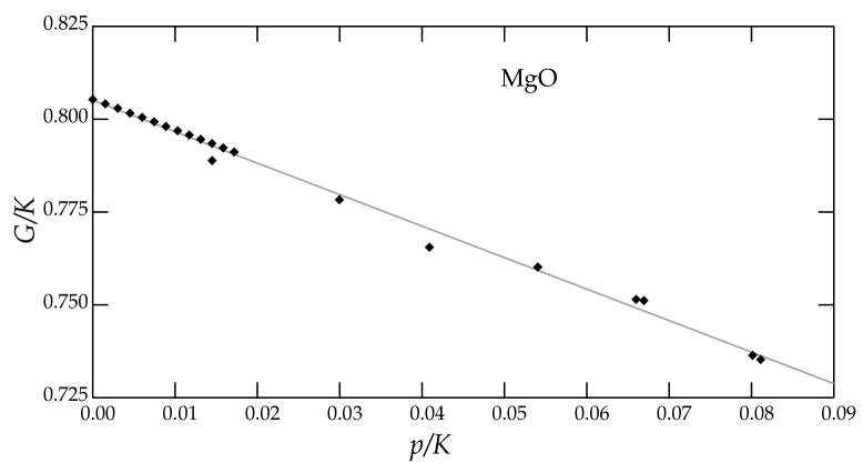
Figure 1: Illustration of the linear dependence of $G/K$ on $p/K$ to 20 GPa pressure, for the adiabatic bulk modulus $K$ of periclase (MgO) using data from Jackson & Niesler (1982), Sinogeikin & Bass (2000), and Zha et al. (2000).

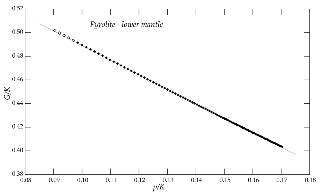
Figure 2: Illustration of the linear dependence of $G/K$ on $p/K$ for a pyrolite composition lower mantle mineral assemblage from Gréaux et al. (2019). The open symbols indicate the zone where some residual garnet may be present.

The linear relation also provides a good description of the properties of mineral assemblages. We illustrate the results for the Earth’s lower mantle using the model developed by Gréaux et al. (2019) in Figure 2. The dominant minerals are bridgmanite and ferropericlase, and some residual majorite garnet is present at the top of the lower mantle where there is a slight deviation from the linear trend. Although the linear form works well over a large range of pressures (up to 140 GPa for the lower mantle), Burakovsky et al. (2004) suggest that (14) should be modified with a slowly-varying pressure dependence for $b$ to allow a match to the expectation for infinite pressure.

The combination of the strain energy development (7) with the identification of moduli (13) and the relation (14) provides a flexible way of extending nonlinear elastic effects to a compressed state, whilst retaining complex shear behaviour for finite strains.

3 Anisotropic materials under pressure

Many natural materials such as wood and tissues show distinct anisotropy in their properties. Most minerals have significant anisotropy, and its only in aggregate that much of the Earth appears to have nearly isotropic properties. For the description of the behaviour of materials under strong compression it is therefore desirable to be able to provide a full description of the anisotropic behaviour.

In the general anisotropic situation the directions of the principal stretches do not remain constant and so their variation has to be taken into account in any formulation. Even so it is possible to express the strain energy $W$ in terms of $J$ and the normalised deformation gradient $\mathbf{F}^{*}$ as $W(\mathbf{F})=W^{*}(J,\mathbf{F}^{*})$. With this representation the Cauchy stress tensor $\boldsymbol{\sigma}$ is given by

$$\boldsymbol{\sigma}=\frac{1}{J}\mathbf{F}\frac{\partial W}{\partial\mathbf{F}}=\frac{\partial W^{*}}{\partial J}\mathbf{I}+\frac{1}{J}\left[\mathbf{F}^{*}\frac{\partial W^{*}}{\partial\mathbf{F}^{*}}-\textstyle{\frac{1}{3}}\displaystyle\mathrm{tr}\left\{\mathbf{F}^{*}\frac{\partial W^{*}}{\partial\mathbf{F}^{*}}\right\}\mathbf{I}\right].$$ (16)

Hence in asimilar way to the isotropic case above we can make a separation into pressure dependence and shear deformations.

For orthotropic materials, Latorre & Montáns (2017) have split the strain energy into an isotropic and a specifically anisotropic part. Such an approach may well be suitable for small compressions, but when we want to include strong compression we should allow for volume dependence of all the components. Building on the approach used for isotropy we look to combine a volumetric component with equivoluminal term modulated by a function of relative volume. We use the equivoluminal equivalents of the Seth-Hill measures (e.g., Miehe & Lambrecht, 2001)

$${\mathbf{E}}^{*}_{q}(\mathbf{U}^{*})=\begin{cases}\frac{1}{q}(\mathbf{U}^{*q}-\mathbf{I})&\text{if}\ q\neq 0,\\ \ln{\mathbf{U}^{*}}&\text{if}\ q=0.\end{cases}$$ (17)

and construct a strain energy function

$$W^{*}(J,\mathbf{F}^{*})=\Phi(J)+\sum_{q}S_{q}(J)W_{q}(\mathbf{E}^{*}_{q}).$$ (18)

Then in terms of the equivoluminal strain $\mathbf{E}^{*}=\mathbf{E}_{2}^{*}=\textstyle{\frac{1}{2}}\displaystyle(\mathbf{U}^{*2}-\mathbf{I})$,

$$\mathbf{F}^{*}\frac{\partial W^{*}}{\partial\mathbf{F}^{*}}=\mathbf{F}^{*}\frac{\partial}{\partial\mathbf{E}^{*}}\sum_{q}S_{q}(J)W_{q}(\mathbf{E}^{*}_{q})\mathbf{F}^{*T}=\mathbf{F}^{*}\sum_{q}\frac{\partial S_{q}(J)}{\partial\mathbf{F}^{*}}W_{q}(\mathbf{E}^{*}_{q})+\mathbf{F}^{*}\sum_{q}S_{q}(J)\frac{\partial W_{q}(\mathbf{E}^{*}_{q})}{\partial\mathbf{E}^{*}}.$$ (19)

The derivative of the functions of relative volume

$$\frac{\partial S_{q}(J)}{\partial\mathbf{F}^{*}}=\frac{\partial S_{q}(J)}{\partial J}\frac{\partial J}{\partial\mathbf{F}^{*}}=J\frac{\partial S_{q}(J)}{\partial J}\mathbf{F}^{*-T}.$$ (20)

Thus, the shear component of the Cauchy stress expression

$$\mathbf{F}^{*}\frac{\partial W^{*}}{\partial\mathbf{F}^{*}}=J\mathbf{I}\sum_{q}\frac{\partial S_{q}(J)}{\partial J}W_{q}(\mathbf{E}^{*}_{q})+\mathbf{F}^{*}\sum_{q}S_{q}(J)\frac{\partial W_{q}(\mathbf{E}^{*}_{q})}{\partial\mathbf{E}_{q}^{*}}\boldsymbol{\mathsf{P}}_{q}.$$ (21)

The fourth order projection tensor $\boldsymbol{\mathsf{P}}_{q}=\partial\mathbf{E}^{*}_{q}/\partial\mathbf{E}^{*}$ is detailed in the Appendix.

The contributions to the stress (16) from the functions $\{S_{q}(J)\}$ are purely hydrostatic, and the shear dependence comes from the choices made for $\{W_{q}(\mathbf{E}^{*})\}$. The evolution of the stress tensor under pressure and the consequent elastic properties can be evaluated by a perturbation treatment around a state of pure compression as in Section 2. As before the bulk modulus $K$ is given by $J\partial^{2}\Phi/\partial J^{2}$.

A simple form for the individual strain energy terms is quadratic:

$$W_{q}=\textstyle{\frac{1}{2}}\displaystyle\mathbf{E}_{q}:\boldsymbol{\mathsf{Z}}_{q}:\mathbf{E}_{q},$$ (22)

where $\boldsymbol{\mathsf{Z}}_{q}$ is a fourth-order stiffness tensor with 21 independent components, and $:$ denotes the double inner product, so that $\mathbf{A}:\mathbf{B}=A_{ij}B_{ji}$. With a sum of a number of Seth-Hill contributions a variety of deformation styles can be produced (e.g., Beex, 2019). In this case for hydrostatic stress $\mathbf{E}^{*}_{q}$ vanishes, and as in the treatment of isotropic elasticity in Section 2 a perturbation treatment about a hydrostatic state simplifies significantly to leave a shear contribution specified by the $S_{q}(J)$.

In this anisotropic development we have introduced separate functions of relative volume for each order of the Seth-Hill strain measures, but simplified forms may be preferable. If the anisotropic properties are consistent with increasing pressure, a suitable strain energy formulation for a material under moderate compression would be

$$W=\Phi(J)+S_{A}(J)\left[\mathbf{E}^{*}_{-1}:\boldsymbol{\mathsf{A}}:\mathbf{E}^{*}_{-1}\right],$$ (23)

in terms of the equivoluminal component of the Almansi strain ${\mathbf{E}}^{*}_{-1}=\mathbf{I}-J^{1/3}\mathbf{U}^{-1}$ (Seth-Hill element of order -1) with a purely volumetric function $S_{A}(J)$. The fourth order tensor $\boldsymbol{\mathsf{A}}$, specifies the shear properties at the rest state $J=1$. The choice of $\Phi(J)$ can be taken from formulations for equation of state, and then $S_{A}(J)$ can be associated in a similar way to the treatment of the shear modulus above.

For materials such as MgO whose anisotropy varies strongly with increasing pressure (Karki et al., 1997) we need to add an additional term to the strain energy, e.g.,

$$S_{B}(J)\left[\mathbf{E}^{*}_{-2}:\boldsymbol{\mathsf{B}}:\mathbf{E}^{*}_{-2}\right],$$ (24)

in terms of the equivoluminal Eulerian strain ${\mathbf{E}}^{*}_{-2}=\mathbf{I}-J^{2/3}\mathbf{U}^{-2}$ (Seth-Hill element of order -2) . The function $S_{B}(J)=0$ at $J=1$, and can be tuned to represent the variations in anisotropy with pressure.

4 Conclusion

We have shown how it is possible to develop formulations of nonlinear elasticity that can accommodate large shear and high compression, by the introduction of a shear function as a function of volume modulating a deviatoric term. For Earth materials, the functional dependence of the shear properties can be guided by the semi-empirical linear relation between shear modulus, bulk modulus and pressure.

For anisotropy a similar development can be made with functions of volume combined with strain energies depending on the the equivoluminal components of the Seth-Hill family of strain tensors. The flexibility of the development provides a means of representing a wide range of isotropic and anisotropic scenarios suitbale for conditions in the Earth’s interior.

The formulation developed in this work has been oriented toward situations with moderate to strong compression, but could also be used for strong expansion with a switch in the style of strain measures employed. For compression, the deviatoric component is best represented using measures depending on strain exponent $q<0$, but in tension $q>0$ is to be preferred (Beex, 2019).

Appendix

The normalised stretch tensor $\mathbf{U}^{*}$ can be written in terms of its eigenvalues, the normalised stretches $\lambda_{i}^{*}=J^{-1/3}\lambda_{i}$, and their associated orthogonal eigenvectors $\mathbf{n}_{i}$ as:

$$\mathbf{U}^{*}=\sum_{i=1}^{3}\lambda_{i}^{*}\mathbf{n}_{i}\mathbf{n}_{i},$$ (A.25)

in terms of the dyadic product of the eigenvectors. The projection tensors $\boldsymbol{\mathsf{P}}_{q}$ introduced in (19) depend on the evolution of strain (Miehe & Lambrecht, 2001; Beex, 2019) and can also be written in terms of the eigen-quantities:

$$\boldsymbol{\mathsf{P}}_{q}=2\frac{\partial\mathbf{E}^{*}_{q}}{\partial\mathbf{E}}=\sum_{i=1}^{3}d^{\{q\}}_{i}\mathbf{n}_{i}\mathbf{n}_{i}\mathbf{n}_{i}\mathbf{n}_{i}+\sum_{r=1}^{3}\sum_{j\neq i}^{3}\vartheta^{\{q\}}_{ij}\big{(}\mathbf{n}_{i}\mathbf{n}_{j}\mathbf{n}_{i}\mathbf{n}_{j}+\mathbf{n}_{i}\mathbf{n}_{j}\mathbf{n}_{j}\mathbf{n}_{i}\big{)}.$$ (A.26)

The coefficients $d_{i}$ depend on the stretches and the order of the strain element $q$

$$d^{\{q\}}_{i}=\lambda_{i}^{*(q-2)}.$$ (A.27)

For three distinct stretches,

$$\vartheta^{\{q\}}_{ij}=\frac{1}{q}\frac{\lambda_{i}^{*q}-\lambda_{j}^{*q}}{\lambda_{i}^{*2}-\lambda_{j}^{*2}}.$$ (A.28)

When two stretches are equal $\lambda^{*}_{a}=\lambda^{*}_{b}\neq\lambda^{*}_{c}$,

$$\vartheta^{\{q\}}_{ab}=\textstyle{\frac{1}{2}}\displaystyle d_{a}.$$ (A.29)

For the hydrostatic case, $\lambda^{*}_{1}=\lambda^{*}_{2}=\lambda^{*}_{3}=1$, the coefficient $\vartheta^{\{q\}}_{ij}=\frac{1}{2}$.

Second derivative projection operators can be defined in a similar way in terms of the stretches and their associated eigenvectors, but now involve sixth-order tensors (Miehe & Lambrecht, 2001; Beex, 2019).

References

- [1]
- [2] eex L.A.A. 2019. Fusing the Seth–Hill strain tensors to fit compressible elastic material responses in the nonlinear regime. Int. J. Mech. Sci. 163 105072
- [3]
- [4] urakovsky L., Preston D.L., Wang Y., 2004. Cold shear modulus and Grüneisen parameter at all densities, Solid State Commun. 132 151–156.
- [5]
- [6] estrade M., Odgen R.W., 2013. On stress-dependent elastic moduli and wave speeds, IMA J. Applied Mathematics, 78, 965–977.
- [7]
- [8] réaux S., Irifune T., Higo Y., Tange Y., Arimoto T., Liu Z., Yamada A., 2019. Sound velocity of CaSiO3 perovskite suggests the presence of basaltic crust in the Earth’s lower mantle. Nature 565 218-221.
- [9]
- [10] ill R., 1968. On constitutive inequalities for simple materials—I. J. Mech. Phys. Solids 16 229–242.
- [11]
- [12] ackson I., Niesler H., 1982. The elasticity of periclase to 3GPa and some geophysical implications. In: Akimoto, S., Manghnani, M.H. (Eds.), High-pressure Research in Geophysics, pp. 93–113, Centre of Academic Publications, Japan.
- [13]
- [14] arki B.B., Stixrude L., Clark S.J., Warren M.C., Ackland G.J., Crain J., 1997. Structure and elasticity of MgO at high pressure. American Mineralogist, 82, 51–-60.
- [15]
- [16] ennett B.L.N., 2017. Towards constitutive equations for the deep Earth. Phys. Earth Planet. Inter. 270, 40–45.
- [17]
- [18] atorre M., Montáns F.J., 2017. WYPIWYG hyperelasticity without inversion formula: application to passive ventricular myocardium. Comput. Struct. 185 47–-58.
- [19]
- [20] iehe C., Lambrecht M., 2001. Algorithms for computation of stresses and elasticity moduli in terms of Seth-Hill’s family of generalized strain tensors. Commun. Numer. Methods Eng. 17, 337–353.
- [21]
- [22] ihai L.A., Goriely A., 2017. How to characterize a nonlinear elastic material? A review on nonlinear constitutive parameters in isotropic finite elasticity. Proc. R. Soc. A 473 20170607.
- [23]
- [24] eth B.R., 1964. Generalized strain measure with application to physical problems. In: Second-Order Effects in Elasticity, Plasticity and Fluid Dynamics, Reiner M, Abir D (eds). Pergamon Press: Oxford, 162–172.
- [25]
- [26] inogeikin S.V., Bass J.D., 2000. Single-crystal elasticity of pyrope and MgO to 20 GPa by Brillouin scattering in the diamond cell. Phys. Earth Planet. Int. 120 43–-62.
- [27]
- [28] pencer A.J.M., 1980. Continuum Mechanics, Longman.
- [29]
- [30] tacey F.D., Davis P.M., 2004. High pressure equations of state with applications to the lower mantle and core. Phys. Earth Planet. Inter. 142 137–184.
- [31]
- [32] tixrude L., Lithgow-Bertelloni C., 2005. Thermodynamics of mantle minerals - I. Physical Properties. Geophys. J. Int., 162, 610–632.
- [33]
- [34] ha C.-S., Mao H.-K., Hemley R.J., 2000. Elasticity of MgO and a primary pressure scale to 55 GPa. PNAS 97 13494–-13499.