Higher-derivative Lorentz-breaking dispersion relations: a thermal description

Abstract

This paper is devoted to study the thermal aspects of a photon gas within the context of Planck-scale-modified dispersion relations. We study the spectrum of radiation and the correction to the Stefan–Boltzmann law in different cases when the Lorentz symmetry is no longer preserved. Explicitly, we examine two models within the context of CPT-even and CPT-odd sectors respectively. To do so, three distinct scenarios of the Universe are considered: the Cosmic Microwave Background (CMB), the electroweak epoch, and the inflationary era. Moreover, the equations of state in these cases turn out to display a dependence on Lorentz-breaking parameters. Finally, we also provide for both theories the analyses of the Helmholtz free energy, the mean energy, the entropy and the heat capacity.

I Introduction

Although the Lorentz invariance is a well-established symmetry of the nature, its possible violation is assumed within many contexts liberati2014astrophysical ; tasson2014we ; hees2016tests . During the last years, the Lorentz symmetry breaking and its possible implications are intensively studied in different scenarios, see f.e. maluf2019antisymmetric ; alfaro2002loop ; pospelov2012lorentz ; mavromatos2007lorentz ; carroll2001noncommutative . As it is known, the Lorentz-breaking parameters are experimentally presumed to be very tiny kostelecky2011data . Nevertheless, this does not imply that they contribute to the physical processes in a negligible manner. Moreover, the presence of Lorentz-violating (LV) higher-derivative additive terms can imply in arising of large quantum corrections collins2004lorentz ; nascimento2018renormalization .

All this clearly motivates us to investigate the higher-derivative LV terms. The first known example of such term was originally introduced by Myers and Pospelov many years ago myers2003ultraviolet . The key feature of this term is that it involves higher (third) derivatives, being proportional to a Lorentz-breaking constant vector and to a small constant parameter (treated as an inverse of some large mass scale). Furthermore, various issues related to them were studied, including its perturbative generation and dispersion relations (for a review on such terms see f.e. kostelecky2009electrodynamics . An exhaustive list of such terms with dimensions up to 6 can be found in kostelecky2019gauge ). It was argued in Ref. mariz2019quantum that a theory involving such a term can be treated consistently as a series in the above-mentioned inverse mass scale.

One of the important issues related to higher-derivative LV theories is certainly their thermodynamical aspects. Studies on the thermodynamics of LV extensions of various field theory models could provide additional information about initial stages of expansion of the Universe, whose size at these stages was compatible with characteristic scales of Lorentz symmetry breaking kostelecky2011data . The methodology for studying the thermodynamical aspects in LV theories has firstly been presented in colladay2004statistical . Since then, various applications of this procedure have been developed casana2008lorentz ; casana2009finite ; gomes2010free ; aa2020lorentz ; maluf2020thermodynamic ; reis2020thermal ; anacleto2018lorentz ; das2009relativistic ; petrov2021bouncing ; reis2021fermions . However, the higher-derivative cases have not been much explored up to now in this context.

In this paper, we follow the procedure proposed by Amelino-Camelia amelino2001testable where the starting point in the study is the LV dispersion relations rather than the Lagrangian formalism of the corresponding field models. Nevertheless, we note that in many cases it is possible to indicate at least some simplified models yielding such dispersion relations. We note that the dispersion relations that we consider in the present manuscript might possibly be used to describe some quantum gravity effects (see discussions in amelino2001testable ), or, at least, they can probably arise in some LV extensions of QED. We consider two examples, CPT-even and CPT-odd ones. In principle, our results involving thermal radiation may be confronted with experimental data as soon as they are available. In this sense, our study might help in the investigation of any trace of the Lorentz violation within cosmological scenarios concerning thermal radiation as the starting point.

II Thermodynamical aspects of CPT-even higher-derivative LV theory

Here, let us consider the higher-derivative LV theories. To study their thermodynamical aspects, we will define the dispersion relations of these theories in which are generally sufficient to obtain various related quantities such as free energy gomes2010free . Our first example is the following dispersion relation bianco2018modified :

$$E^{2}={\bf{k}}^{2}+\sigma^{4}{\bf{k}}^{6}.$$ (1)

Clearly, if we consider $\sigma\rightarrow 0$, the usual dispersion relation $E^{2}={\bf{k}}^{2}$ is recove. Physically, such a relation can arise in Horava-Lifshitz-like theories involving both $z=1$ and $z=3$ terms in the spatial sector, e.g. in a scalar field model characterized by the Lagrangian ${\cal L}=\frac{1}{2}\phi(\Box+\sigma^{4}(\nabla^{2})^{3})\phi$, in a spinor model involving terms with these values of $z$ gomes2018one , and perhaps for some degrees of freedom of a certain LV gauge theory or, a Horava-Lifshitz-like gravity model involving $z=3$ and $z=1$ terms Horava:2009uw . Let us briefly discuss the possible physical significance of these relations. It must be noted that the usual Lorentz-breaking extensions of various field theory models conside within phernomenological context – their full list is given in kostelecky2011data – have rather a different form since they involve the same orders in space and time derivatives until we choose the special form of Lorentz-breaking parameters. More so, the models involving the dispersion relations like (1) can also be regarded for studies of various physical problems; for instance, one of the most important applications of this model has been developed in deFarias:2020iqh where it was used for an investigation of gamma-ray bursts in the Lorentz-breaking context and allowed to estimate the characteristic energy of quantum gravity mass. It is easy to see that the dispersion relation in Eq. (1) gives rise to six solutions. Nevertheless, only one of them allows us to work on a positive defined real spatial momentum. In this sense, we can write the solution of Eq. (1) as being

$${\bf{k}}=\left(\frac{\sqrt[3]{\sqrt{3}\sqrt{4\sigma^{12}+27\sigma^{16}E^{4}}+9\sigma^{8}E^{2}}}{\sqrt[3]{2}\,3^{2/3}\sigma^{4}}-\frac{\sqrt[3]{\frac{2}{3}}}{\sqrt[3]{\sqrt{3}\sqrt{4\sigma^{12}+27\sigma^{16}E^{4}}+9\sigma^{8}E^{2}}}\right)^{1/2}.$$ (2)

Next, we take the advantage of using the formalism of the partition function in order to derive all relevant thermodynamic quantities i.e., Helmholtz free energy, mean energy, entropy and heat capacity. Initially, we calculate the number of accessible states of the system reif1998fundamentals ; gibbs2014elementary ; greiner2012thermodynamics ; callen1998thermodynamics . By definition, it can be represented as

$$\Omega(E)=\frac{\zeta}{(2\pi)^{3}}\int\int\mathrm{d}^{3}{\bf{x}}\,\mathrm{d}^{3}{\bf{k}},$$ (3)

where $\zeta$ is the spin multiplicity whose magnitude in the photon sector is $\zeta=2$ anacleto2018lorentz . More so, Eq. (3) can be rewritten as

$$\Omega(E)=\frac{V}{\pi^{2}}\int^{\infty}_{0}\mathrm{d}{\bf{k}}|{\bf{k}}|^{2},$$ (4)

where $V$ is the volume of the thermal reservoir and the integral measure $\mathrm{d}{\bf{k}}$ is given by

$$\mathrm{d}{\bf{k}}=\frac{\frac{\sqrt[3]{\frac{2}{3}}\left(\frac{54\sqrt{3}\sigma^{16}E^{3}}{\sqrt{4\sigma^{12}+27\sigma^{16}E^{4}}}+18\sigma^{8}E\right)}{3\left(\sqrt{3}\sqrt{4\sigma^{12}+27\sigma^{16}E^{4}}+9\sigma^{8}E^{2}\right)^{4/3}}+\frac{\frac{54\sqrt{3}\sigma^{16}E^{3}}{\sqrt{4\sigma^{12}+27\sigma^{16}E^{4}}}+18\sigma^{8}E}{3\sqrt[3]{2}3^{2/3}\sigma^{4}\left(\sqrt{3}\sqrt{4\sigma^{12}+27\sigma^{16}E^{4}}+9\sigma^{8}E^{2}\right)^{2/3}}}{2\sqrt{\frac{\sqrt[3]{\sqrt{3}\sqrt{4\sigma^{12}+27\sigma^{16}E^{4}}+9\sigma^{8}E^{2}}}{\sqrt[3]{2}3^{2/3}\sigma^{4}}-\frac{\sqrt[3]{\frac{2}{3}}}{\sqrt[3]{\sqrt{3}\sqrt{4\sigma^{12}+27\sigma^{16}E^{4}}+9\sigma^{8}E^{2}}}}}\mathrm{d}E.$$ (5)

Next, we substitute $(\ref{dr1})$ and $(\ref{vol1})$ in $(\ref{ms1})$, which yields

$$\begin{split}\Omega(\sigma)=\frac{V}{\pi^{2}}\int^{\infty}_{0}&\left(\frac{\sqrt[3]{\frac{2}{3}}\left(\frac{54\sqrt{3}\sigma^{16}E^{3}}{\sqrt{4\sigma^{12}+27\sigma^{16}E^{4}}}+18\sigma^{8}E\right)}{3\left(\sqrt{3}\sqrt{4\sigma^{12}+27\sigma^{16}E^{4}}+9\sigma^{8}E^{2}\right)^{4/3}}\right.\\ &\left.+\frac{\frac{54\sqrt{3}\sigma^{16}E^{3}}{\sqrt{4\sigma^{12}+27\sigma^{16}E^{4}}}+18\sigma^{8}E}{3\sqrt[3]{2}3^{2/3}\sigma^{4}\left(\sqrt{3}\sqrt{4\sigma^{12}+27\sigma^{16}E^{4}}+9\sigma^{8}E^{2}\right)^{2/3}}\right)\\ &\times\sqrt{\frac{\sqrt[3]{\sqrt{3}\sqrt{4\sigma^{12}+27\sigma^{16}E^{4}}+9\sigma^{8}E^{2}}}{\sqrt[3]{2}3^{2/3}\sigma^{4}}-\frac{\sqrt[3]{\frac{2}{3}}}{\sqrt[3]{\sqrt{3}\sqrt{4\sigma^{12}+27\sigma^{16}E^{4}}+9\sigma^{8}E^{2}}}}\,\mathrm{d}E,\end{split}$$ (6)

and, therefore, we can explicitly write down the partition function in a manner similar to Refs. anacleto2018lorentz ; maluf2020casimir as follows:

$$\begin{split}\mathrm{ln}\left[Z(\beta,\Gamma,\sigma)\right]=&-\frac{V}{\pi^{2}}\int^{\infty}_{0}\left(\frac{\sqrt[3]{\frac{2}{3}}\left(\frac{54\sqrt{3}\sigma^{16}E^{3}}{\sqrt{4\sigma^{12}+27\sigma^{16}E^{4}}}+18\sigma^{8}E\right)}{3\left(\sqrt{3}\sqrt{4\sigma^{12}+27\sigma^{16}E^{4}}+9\sigma^{8}E^{2}\right)^{4/3}}\right.\\ &\left.+\frac{\frac{54\sqrt{3}\sigma^{16}E^{3}}{\sqrt{4\sigma^{12}+27\sigma^{16}E^{4}}}+18\sigma^{8}E}{3\sqrt[3]{2}3^{2/3}\sigma^{4}\left(\sqrt{3}\sqrt{4\sigma^{12}+27\sigma^{16}E^{4}}+9\sigma^{8}E^{2}\right)^{2/3}}\right)\times\mathrm{ln}\left(1-e^{-\beta E}\right)\\ &\times\sqrt{\frac{\sqrt[3]{\sqrt{3}\sqrt{4\sigma^{12}+27\sigma^{16}E^{4}}+9\sigma^{8}E^{2}}}{\sqrt[3]{2}3^{2/3}\sigma^{4}}-\frac{\sqrt[3]{\frac{2}{3}}}{\sqrt[3]{\sqrt{3}\sqrt{4\sigma^{12}+27\sigma^{16}E^{4}}+9\sigma^{8}E^{2}}}}\,\mathrm{d}E,\end{split}$$ (7)

where $\beta=1/(k_{B}T)$ is the inverse of the temperature. From Eq. (7), the thermodynamic functions can be derived. It is important to mention that all our calculations will provide the values of these functions per volume $V$. The thermal functions of interest are defined as

$$\begin{split}&F(\beta,\sigma)=-\frac{1}{\beta}\mathrm{ln}\left[Z(\beta,\sigma)\right],\\ &U(\beta,\sigma)=-\frac{\partial}{\partial\beta}\mathrm{ln}\left[Z(\beta,\sigma)\right],\\ &S(\beta,\sigma)=k_{B}\beta^{2}\frac{\partial}{\partial\beta}F(\beta,\sigma),\\ &C_{V}(\beta,\sigma)=-k_{B}\beta^{2}\frac{\partial}{\partial\beta}U(\beta,\sigma).\end{split}$$ (8)

Primarily, let us focus on the mean energy

$$U(\beta,\sigma) = \frac{V}{\pi^{2}}\int^{\infty}_{0}\mathrm{d}EE\left(\frac{\sqrt[3]{\frac{2}{3}}\left(\frac{54\sqrt{3}\sigma^{16}E^{3}}{\sqrt{4\sigma^{12}+27\sigma^{16}E^{4}}}+18\sigma^{8}E\right)}{3\left(\sqrt{3}\sqrt{4\sigma^{12}+27\sigma^{16}E^{4}}+9\sigma^{8}E^{2}\right)^{4/3}}\right.$$ (9)

$$+ \left.\frac{\frac{54\sqrt{3}\sigma^{16}E^{3}}{\sqrt{4\sigma^{12}+27\sigma^{16}E^{4}}}+18\sigma^{8}E}{3\sqrt[3]{2}3^{2/3}\sigma^{4}\left(\sqrt{3}\sqrt{4\sigma^{12}+27\sigma^{16}E^{4}}+9\sigma^{8}E^{2}\right)^{2/3}}\right)\times\frac{e^{-\beta E}}{\left(1-e^{-\beta E}\right)}$$

$$\times \sqrt{\frac{\sqrt[3]{\sqrt{3}\sqrt{4\sigma^{12}+27\sigma^{16}E^{4}}+9\sigma^{8}E^{2}}}{\sqrt[3]{2}\cdot 3^{2/3}\sigma^{4}}-\frac{\sqrt[3]{\frac{2}{3}}}{\sqrt[3]{\sqrt{3}\sqrt{4\sigma^{12}+27\sigma^{16}E^{4}}+9\sigma^{8}E^{2}}}}\,$$

which implies the following spectral radiance:

$$\chi(\sigma,\nu) = \frac{h\nu}{\pi^{2}}\left(\frac{\sqrt[3]{\frac{2}{3}}\left(\frac{54\sqrt{3}\sigma^{16}(h\nu)^{3}}{\sqrt{4\sigma^{12}+27\sigma^{16}(h\nu)^{4}}}+18\sigma^{8}(h\nu)\right)}{3\left(\sqrt{3}\sqrt{4\sigma^{12}+27\sigma^{16}(h\nu)^{4}}+9\sigma^{8}(h\nu)^{2}\right)^{4/3}}\right.$$

$$+ \left.\frac{\frac{54\sqrt{3}\sigma^{16}(h\nu)^{3}}{\sqrt{4\sigma^{12}+27\sigma^{16}(h\nu)^{4}}}+18\sigma^{8}(h\nu)}{3\sqrt[3]{2}3^{2/3}\sigma^{4}\left(\sqrt{3}\sqrt{4\sigma^{12}+27\sigma^{16}(h\nu)^{4}}+9\sigma^{8}(h\nu)^{2}\right)^{2/3}}\right)\times\frac{e^{-\beta(h\nu)}}{\left(1-e^{-\beta(h\nu)}\right)}$$

$$\times \sqrt{\frac{\sqrt[3]{\sqrt{3}\sqrt{4\sigma^{12}+27\sigma^{16}(h\nu)^{4}}+9\sigma^{8}(h\nu)^{2}}}{\sqrt[3]{2}3^{2/3}\sigma^{4}}-\frac{\sqrt[3]{\frac{2}{3}}}{\sqrt[3]{\sqrt{3}\sqrt{4\sigma^{12}+27\sigma^{16}(h\nu)^{4}}+9\sigma^{8}(h\nu)^{2}}}}\,.$$

Here, $E=h\nu$ where $h$ is the well-known Planck constant and $\nu$ is the frequency. Now, let us examine how the parameter $\sigma$ affects the spectral radiance of our theory. In addition, it must be noted that, despite of showing explicitly the constants $h,k_{B}$, to obtain the following calculations, we choose them as being $h=k_{B}=1$. At the beginning, we examine how the black body spectra can be modified by the parameter $\sigma$. Moreover, we consider three different configurations of temperatures for our system, namely, CMB ($\mathrm{T}=10^{-13}$ GeV), electroweak epoch ($\mathrm{T}=10^{3}$ GeV) and inflationary era ($\mathrm{T}=10^{13}$ GeV).

The results displayed at Fig. 1 show that the only one configuration of the black body radiation took a proper place in a prominent manner (in terms of shape of the curve) – it was with the CMB temperature. Furthermore, taking into account the electroweak scenario, we see that the graphics started to increase reaching maxima peaks and, then, tended to attenuate their values until having a constant behavior. On the other hand, to the inflationary temperature, the plots show a behavior closer to Wien’s energy density distribution zettili2003quantum .

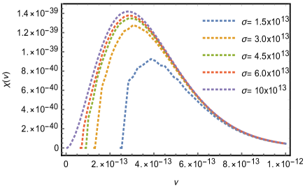
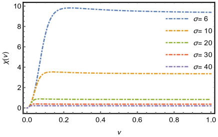
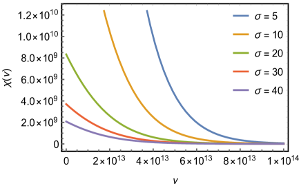
Figure 1: The plots exhibit the spectral radiance $\chi(\nu)$ changing for different values of frequency $\nu$ and the Lorentz-breaking parameter $\sigma$ (its unit is GeV^-1). The top left (dotted) is the configuration to the cosmic microwave background, i.e., $\beta=10^{13}$ GeV^-1; the top right (dot-dashed) is ascribed to the electroweak configuration, i.e., $\beta=10^{-3}$ GeV^-1; the bottom plot shows the black body radiation to the inflationary period of the Universe, i.e., $\beta=10^{-13}$ GeV^-1.

Another interesting aspect to be verified is the correction to the Stefan–Boltzmann law ascribed to the parameter $\sigma$. In order to do this, let us define the constant:

$$\tilde{\alpha}\equiv U(\beta,\sigma)\beta^{4}.$$ (11)

As it can easily be noted, the above expressions are unsolvable analytically. Thereby, the calculations will be performed numerically. Analogously, we regard the same previous configurations of temperature and the plots are exhibited in Fig. 2. For the CMB temperature, the curve exhibits a constant behavior of $\alpha$. Moreover, to the electroweak epoch, we have a decreasing function $\tilde{\alpha}$ when $\sigma$ started to increase. The inflationary era, on the other hand, shows an increasing function of $\tilde{\alpha}$ for positive changes of $\sigma$. To this latter case, for $\tilde{\alpha}<20$, the system seems to show instability. Next, we shall acquire all the remaining thermodynamic properties in what follows.

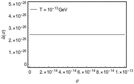
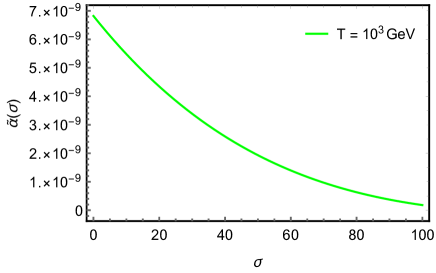
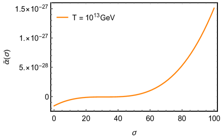
Figure 2: The figure shows the correction to the Stefan–Boltzmann law ascribed to parameter $\tilde{\alpha}$ as a function of $\sigma$ (its unit is GeV^-1) for the temperatures of cosmic microwave background (top left), electroweak scenario (top right) and the early inflationary universe (bottom).

Using the expressions above, we can first obtain the Helmholtz free energy as being

$$F(\beta,\sigma) = \frac{V}{\beta\pi^{2}}\int^{\infty}_{0}\left(\frac{\sqrt[3]{\frac{2}{3}}\left(\frac{54\sqrt{3}\sigma^{16}E^{3}}{\sqrt{4\sigma^{12}+27\sigma^{16}E^{4}}}+18\sigma^{8}E\right)}{3\left(\sqrt{3}\sqrt{4\sigma^{12}+27\sigma^{16}E^{4}}+9\sigma^{8}E^{2}\right)^{4/3}}\right.$$

$$+ \left.\frac{\frac{54\sqrt{3}\sigma^{16}E^{3}}{\sqrt{4\sigma^{12}+27\sigma^{16}E^{4}}}+18\sigma^{8}E}{3\sqrt[3]{2}3^{2/3}\sigma^{4}\left(\sqrt{3}\sqrt{4\sigma^{12}+27\sigma^{16}E^{4}}+9\sigma^{8}E^{2}\right)^{2/3}}\right)\times\mathrm{ln}\left(1-e^{-\beta E}\right)$$

$$\times \sqrt{\frac{\sqrt[3]{\sqrt{3}\sqrt{4\sigma^{12}+27\sigma^{16}E^{4}}+9\sigma^{8}E^{2}}}{\sqrt[3]{2}3^{2/3}\sigma^{4}}-\frac{\sqrt[3]{\frac{2}{3}}}{\sqrt[3]{\sqrt{3}\sqrt{4\sigma^{12}+27\sigma^{16}E^{4}}+9\sigma^{8}E^{2}}}}\,\mathrm{d}E,$$

the entropy

$$S(\beta,\sigma) = -\frac{Vk_{B}}{\pi^{2}}\int^{\infty}_{0}\left(\frac{\sqrt[3]{\frac{2}{3}}\left(\frac{54\sqrt{3}\sigma^{16}E^{3}}{\sqrt{4\sigma^{12}+27\sigma^{16}E^{4}}}+18\sigma^{8}E\right)}{3\left(\sqrt{3}\sqrt{4\sigma^{12}+27\sigma^{16}E^{4}}+9\sigma^{8}E^{2}\right)^{4/3}}\right.$$

$$+ \left.\frac{\frac{54\sqrt{3}\sigma^{16}E^{3}}{\sqrt{4\sigma^{12}+27\sigma^{16}E^{4}}}+18\sigma^{8}E}{3\sqrt[3]{2}3^{2/3}\sigma^{4}\left(\sqrt{3}\sqrt{4\sigma^{12}+27\sigma^{16}E^{4}}+9\sigma^{8}E^{2}\right)^{2/3}}\right)\times\mathrm{ln}\left(1-e^{-\beta E}\right)$$

$$\times \sqrt{\frac{\sqrt[3]{\sqrt{3}\sqrt{4\sigma^{12}+27\sigma^{16}E^{4}}+9\sigma^{8}E^{2}}}{\sqrt[3]{2}3^{2/3}\sigma^{4}}-\frac{\sqrt[3]{\frac{2}{3}}}{\sqrt[3]{\sqrt{3}\sqrt{4\sigma^{12}+27\sigma^{16}E^{4}}+9\sigma^{8}E^{2}}}}$$

$$+ \frac{V\beta k_{B}}{\pi^{2}}\int^{\infty}_{0}E\left(\frac{\sqrt[3]{\frac{2}{3}}\left(\frac{54\sqrt{3}\sigma^{16}E^{3}}{\sqrt{4\sigma^{12}+27\sigma^{16}E^{4}}}+18\sigma^{8}E\right)}{3\left(\sqrt{3}\sqrt{4\sigma^{12}+27\sigma^{16}E^{4}}+9\sigma^{8}E^{2}\right)^{4/3}}\right.$$

$$+ \left.\frac{\frac{54\sqrt{3}\sigma^{16}E^{3}}{\sqrt{4\sigma^{12}+27\sigma^{16}E^{4}}}+18\sigma^{8}E}{3\sqrt[3]{2}3^{2/3}\sigma^{4}\left(\sqrt{3}\sqrt{4\sigma^{12}+27\sigma^{16}E^{4}}+9\sigma^{8}E^{2}\right)^{2/3}}\right)\times\frac{e^{-\beta E}}{1-e^{-\beta E}}$$

$$\times \sqrt{\frac{\sqrt[3]{\sqrt{3}\sqrt{4\sigma^{12}+27\sigma^{16}E^{4}}+9\sigma^{8}E^{2}}}{\sqrt[3]{2}3^{2/3}\sigma^{4}}-\frac{\sqrt[3]{\frac{2}{3}}}{\sqrt[3]{\sqrt{3}\sqrt{4\sigma^{12}+27\sigma^{16}E^{4}}+9\sigma^{8}E^{2}}}}\,\mathrm{d}E,$$

and, lastly, the heat capacity

$$C_{V}(\beta,\sigma) = \frac{Vk_{B}\beta^{2}}{\pi^{2}}\int^{\infty}_{0}E^{2}\left(\frac{\sqrt[3]{\frac{2}{3}}\left(\frac{54\sqrt{3}\sigma^{16}E^{3}}{\sqrt{4\sigma^{12}+27\sigma^{16}E^{4}}}+18\sigma^{8}E\right)}{3\left(\sqrt{3}\sqrt{4\sigma^{12}+27\sigma^{16}E^{4}}+9\sigma^{8}E^{2}\right)^{4/3}}\right.$$

$$+ \left.\frac{\frac{54\sqrt{3}\sigma^{16}E^{3}}{\sqrt{4\sigma^{12}+27\sigma^{16}E^{4}}}+18\sigma^{8}E}{3\sqrt[3]{2}3^{2/3}\sigma^{4}\left(\sqrt{3}\sqrt{4\sigma^{12}+27\sigma^{16}E^{4}}+9\sigma^{8}E^{2}\right)^{2/3}}\right)\times\frac{e^{-2\beta E}}{(1-e^{-\beta E})^{2}}$$

$$\times \sqrt{\frac{\sqrt[3]{\sqrt{3}\sqrt{4\sigma^{12}+27\sigma^{16}E^{4}}+9\sigma^{8}E^{2}}}{\sqrt[3]{2}3^{2/3}\sigma^{4}}-\frac{\sqrt[3]{\frac{2}{3}}}{\sqrt[3]{\sqrt{3}\sqrt{4\sigma^{12}+27\sigma^{16}E^{4}}+9\sigma^{8}E^{2}}}}$$

$$+ \frac{Vk_{B}\beta^{2}}{\pi^{2}}\int^{\infty}_{0}E^{2}\left(\frac{\sqrt[3]{\frac{2}{3}}\left(\frac{54\sqrt{3}\sigma^{16}E^{3}}{\sqrt{4\sigma^{12}+27\sigma^{16}E^{4}}}+18\sigma^{8}E\right)}{3\left(\sqrt{3}\sqrt{4\sigma^{12}+27\sigma^{16}E^{4}}+9\sigma^{8}E^{2}\right)^{4/3}}\right.$$

$$+ \left.\frac{\frac{54\sqrt{3}\sigma^{16}E^{3}}{\sqrt{4\sigma^{12}+27\sigma^{16}E^{4}}}+18\sigma^{8}E}{3\sqrt[3]{2}3^{2/3}\sigma^{4}\left(\sqrt{3}\sqrt{4\sigma^{12}+27\sigma^{16}E^{4}}+9\sigma^{8}E^{2}\right)^{2/3}}\right)\times\frac{e^{-\beta E}}{1-e^{-\beta E}}$$

$$\times \sqrt{\frac{\sqrt[3]{\sqrt{3}\sqrt{4\sigma^{12}+27\sigma^{16}E^{4}}+9\sigma^{8}E^{2}}}{\sqrt[3]{2}3^{2/3}\sigma^{4}}-\frac{\sqrt[3]{\frac{2}{3}}}{\sqrt[3]{\sqrt{3}\sqrt{4\sigma^{12}+27\sigma^{16}E^{4}}+9\sigma^{8}E^{2}}}}\,\mathrm{d}E.$$

Their behaviors are shown in Figs. 5, 6, and 7 respectively. Moreover, the thermal quantities were also calculated oliveira2019thermodynamic ; oliveira2020thermodynamic ; reis2020does ; lobo2020effects ; lobo2020thermal ; amelino2017thermal into different contexts. In the context of CMB, all of them turned out to have no contribution to our calculations. For Helmholtz free energy, we obtained decreasing curves with an expressive curvature when $\sigma$ increases for both electroweak and inflationary cases. The entropy, on the other hand, showed a decreasing behavior for different values of $\sigma$ for both electroweak and inflationary cases. It is worth mentioning that such behavior does not imply an instability since the entropy is still an increasing function when it is analyzed against the temperature for fixed values of $\sigma$ – as it should be. Lastly, the heat capacity exhibited a strong increasing behavior when $\sigma$ started to change for both cases as well, i.e., the CMB and the inflationary temperatures. In principle, this fact might signalize the possibility of some phase transition at some large $\sigma$; nevertheless, this hypothesis requires further investigation.

Whenever we are dealing with the thermodynamic systems, one question naturally arises: what is the form of the equation of state when the parameter $\sigma$, which characterizes the magnitude of Lorentz symmetry breaking, is taken into account? To answer such a question, we must start with the following relation:

$$\mathrm{d}F=-S\,\mathrm{d}T-p\,\mathrm{d}V,$$ (15)

which, immediately, implies

$$p=-\left(\frac{\partial F}{\partial V}\right)_{T} = -\frac{1}{\beta\pi^{2}}\int^{\infty}_{0}\left(\frac{\sqrt[3]{\frac{2}{3}}\left(\frac{54\sqrt{3}\sigma^{16}E^{3}}{\sqrt{4\sigma^{12}+27\sigma^{16}E^{4}}}+18\sigma^{8}E\right)}{3\left(\sqrt{3}\sqrt{4\sigma^{12}+27\sigma^{16}E^{4}}+9\sigma^{8}E^{2}\right)^{4/3}}\right.$$

$$+ \left.\frac{\frac{54\sqrt{3}\sigma^{16}E^{3}}{\sqrt{4\sigma^{12}+27\sigma^{16}E^{4}}}+18\sigma^{8}E}{3\sqrt[3]{2}3^{2/3}\sigma^{4}\left(\sqrt{3}\sqrt{4\sigma^{12}+27\sigma^{16}E^{4}}+9\sigma^{8}E^{2}\right)^{2/3}}\right)\times\mathrm{ln}\left(1-e^{-\beta E}\right)$$

$$\times \sqrt{\frac{\sqrt[3]{\sqrt{3}\sqrt{4\sigma^{12}+27\sigma^{16}E^{4}}+9\sigma^{8}E^{2}}}{\sqrt[3]{2}3^{2/3}\sigma^{4}}-\frac{\sqrt[3]{\frac{2}{3}}}{\sqrt[3]{\sqrt{3}\sqrt{4\sigma^{12}+27\sigma^{16}E^{4}}+9\sigma^{8}E^{2}}}}\,\mathrm{d}E.$$

Here, we focus on the study of the behavior of pressure – which leads to the equation of states. After introducing new dimensionless variable $t=\sigma E$, we get

$$p = \frac{1}{\sigma^{3}\beta\pi^{2}}\int_{0}^{\infty}\mathrm{d}t\,\mathrm{ln}(1-e^{-\frac{\beta}{\sigma}t})F(t);$$

$$F(t) = -2^{1/6}3^{-7/6}\frac{t}{\sqrt{4+27t^{4}}}\left[(\chi(t))^{-1/3}+\frac{1}{\sqrt[3]{18}}(\chi(t))^{1/3}\right]\cdot\sqrt{\frac{(\chi(t))^{2/3}-12^{1/3}}{(\chi(t))^{1/3}}};$$

$$\chi(t) = \sqrt{3}\cdot\sqrt{4+27t^{4}}+9t^{2}.$$ (17)

With these above expressions, let us examine some limits. Initially, at the very high temperature limit, namely $\frac{\beta}{\sigma}=\frac{1}{\sigma T}\ll 1$, we perform the expansion in the Taylor series. After that, only the first two terms are considered, which yields $p=\frac{1}{\sigma^{3}\beta\pi^{2}}\frac{\beta}{\sigma}\int_{0}^{\infty}\mathrm{d}tF(t)t=\frac{c_{h}}{\sigma^{4}\pi^{2}}$, where $c_{h}=\int_{0}^{\infty}\mathrm{d}tF(t)t$, i.e., at $T\to\infty$ ($\beta\to 0$), the pressure tends to a constant. Such behavior is displayed in Fig. 3; next, at the natural limit of low Lorentz symmetry breaking or low temperature, one has $\frac{\beta}{\sigma}\gg 1$. In this case, the exponential is strongly suppressed, and one has $p=\frac{c_{l}}{\sigma^{3}\beta\pi^{2}}$, where $c_{l}=\int_{0}^{\infty}\mathrm{d}tF(t)$, i.e., the pressure grows linearly with the temperature. Thereby, its corresponding behavior is shown in Fig. 4.

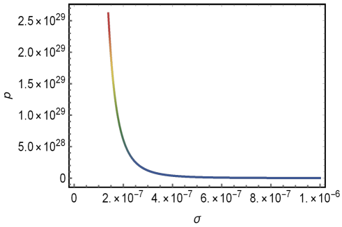
Figure 3: This figure shows the behavior of the equation of states when the high temperature limit, namely $\frac{\beta}{\sigma}\ll 1$, is taken into account.

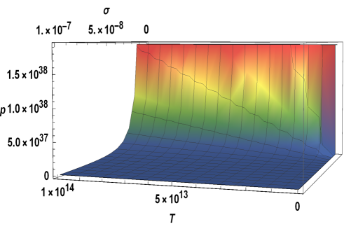
Figure 4: This figure shows the behavior of the equation of states when the low temperature limit, namely $\frac{\beta}{\sigma}\gg 1$, is taken into account.

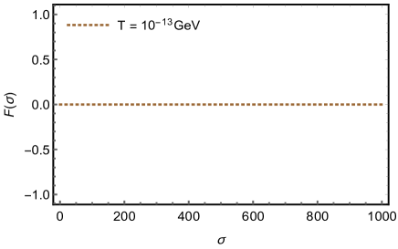
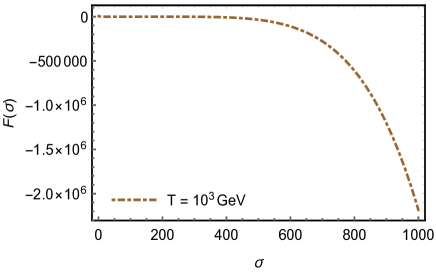
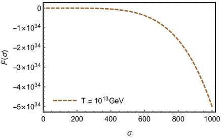
Figure 5: The figure shows the modification of the Helmholtz free energy $F(\sigma)$ due to the parameter $\sigma$ (its unit is GeV^-1) considering the temperatures of cosmic microwave background (top left), electroweak scenario (top right) and the early inflationary universe (bottom).

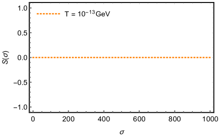
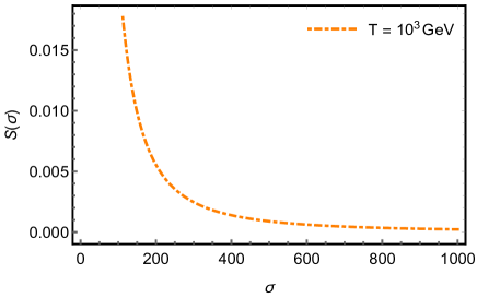
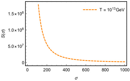
Figure 6: The plots show the modification to the entropy $S(\sigma)$ as a function of $\sigma$ (its unit is GeV^-1) considering the temperatures of cosmic microwave background (top left), electroweak scenario (top right), and the early inflationary universe (bottom).

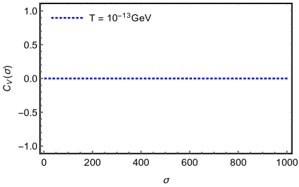
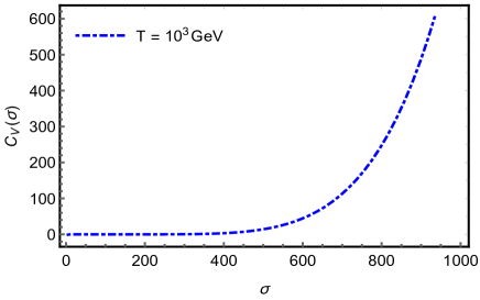
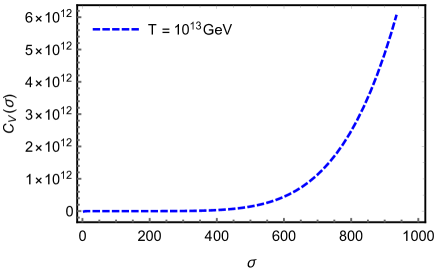
Figure 7: The plots show the modification to the heat capacity $C_{V}(\sigma)$ as a function of $\sigma$ (its unit is GeV^-1) considering the temperatures of cosmic microwave background (top left), electroweak scenario (top right), and the early inflationary universe (bottom).

III Thermodynamical aspects of CPT-odd higher-derivative LV theory

In this section, let us consider the theory described by the following dispersion relation rosati2015planck :

$$E^{2}+\alpha lE^{3}+\beta lE{\bf{k}}^{2}={\bf k}^{2}+m^{2}.$$ (18)

where $l$ is a parameter characterizing the intensity of the Lorentz symmetry breaking. It is clear that in the limit $l\rightarrow 0$, the standard massive dispersion relation $E^{2}={\bf{k}}^{2}+m^{2}$ is recovered. Such a relation, being similar to relations studied in Ref. amelino2001testable , can arise e.g. in a scalar field theory with the higher-derivative quadratic Lagrangian of the scalar field looking like ${\cal L}=\frac{1}{2}\phi(\Box+m^{2}+\rho^{\mu\nu\lambda}\partial_{\mu}\partial_{\nu}\partial_{\rho})\phi$, with $\rho^{\mu\nu\lambda}$ being a completely symmetric third-rank tensor whose only non-zero components are $\rho^{000}=\beta l$, and $\rho^{0ij}=\frac{1}{3}\alpha l\delta^{ij}$. In principle, it is natural to expect that such a relation, in the massless case, can also arise in a specific higher-derivative LV extension of QED. In particular, the dispersion relation displayed in Eq. (18) can be applied to understand how Planck-scale effects may affect translation transformations. This is relevant due to the fact that it carries the information on the distance between source and detector, and it factors in the interplay between quantum-spacetime effects and the curvature of spacetime amelino2016icecube ; rosati2015planck . In the literature, some propositions are addressed in the context of gamma-ray-burst neutrinos and photons amelino2017vacuo , and IceCube and GRB neutrinos amelino2016icecube .

Thereby, we restrict ourselves to a particular massless case, i.e., we set $m=0,\alpha=1$ and $\beta=1$. In this sense, it is convenient to rewrite Eq. (18) as

$${\bf{k}}^{2}=\frac{E^{2}+lE^{3}}{1-lE},$$ (19)

where, analogously with the previous section, the accessible states can be derived:

$$\bar{\Omega}(l)=\frac{\Gamma}{2\pi^{2}}\int^{\infty}_{0}\left(\frac{E^{2}+lE^{3}}{1-lE}\right)^{1/2}\left[\frac{(2E+3lE^{2})(1-lE)+l(E^{2}+lE^{3})}{(1-lE)^{2}}\right]\mathrm{d}E.$$ (20)

With this, we are able to write down the corresponding partition function as follows

$$\mathrm{ln}\left[\bar{Z}(\beta,l)\right]=$$

$$= -\frac{\Gamma}{\pi^{2}}\int^{\infty}_{0}\left(\frac{E^{2}+lE^{3}}{1-lE}\right)^{1/2}\left[\frac{(2E+3lE^{2})(1-lE)+l(E^{2}+lE^{3})}{(1-lE)^{2}}\right]\mathrm{ln}\left(1-e^{-\beta E}\right)\mathrm{d}E.$$

Using Eq. (III), we can obtain the thermodynamic functions per volume $\Gamma$ as well. Here, we provide the calculation of Helmholtz free energy $\bar{F}(\beta,l)$, mean energy $\bar{U}(\beta,l)$, entropy $\bar{S}(\beta,l)$, and heat capacity $\bar{C}_{V}(\beta,l)$. Let us start with the mean energy

$$\bar{U}(\beta,l)=\frac{1}{\pi^{2}}\int^{\infty}_{0}E\left(\frac{E^{2}+lE^{3}}{1-lE}\right)^{1/2}\left[\frac{(2E+3lE^{2})(1-lE)+l(E^{2}+lE^{3})}{(1-lE)^{2}}\right]\frac{e^{-\beta E}}{\left(1-e^{-\beta E}\right)}\mathrm{d}E,$$ (22)

which implies the spectral radiance given by:

$$\bar{\chi}(l,\nu) = (h\nu)\left(\frac{(h\nu)^{2}+l(h\nu)^{3}}{1-l(h\nu)}\right)^{1/2}\left[\frac{(2(h\nu)+3l(h\nu)^{2})(1-l(h\nu))+l((h\nu)^{2}+l(h\nu)^{3})}{(1-l(h\nu))^{2}}\right]\times$$ (23)

$$\times \frac{e^{-\beta(h\nu)}}{\left(1-e^{-\beta(h\nu)}\right)}.$$

The respective plots of these thermal quantities are presented in Fig. 8. Here, we show the black body radiation spectra for different values of $l$ corresponding to the Cosmic Microwave Background, electroweak epoch and inflationary era of the Universe. Moreover, the black body radiation shape is maintained for the three of them, differently what happened in our first example in the previous section. Note that when $l\rightarrow 0$, we recover the usual radiation constant of the Stefan–Boltzmann law, namely, $u_{SB}=\alpha T^{4}$. In other words, we have

$$\alpha=\frac{1}{\pi^{2}}\int^{\infty}_{0}\frac{E^{3}\,e^{-\beta E}}{\left(1-e^{-\beta E}\right)}\mathrm{d}E=\frac{\pi^{2}}{15}.$$ (24)

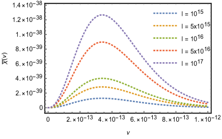
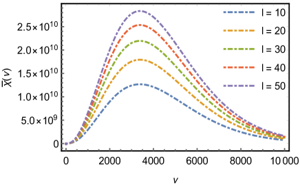
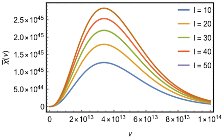
Figure 8: The plots show how the spectral radiance $\bar{\chi}(\nu)$ changes as a function of frequency $\nu$ and $l(\text{whose dimension is}\,\,m\cdot kg^{-1/2}\cdot s^{-1})$ for three different cases. The top left (dotted) is configuration to the cosmic microwave background, i.e., $\beta=10^{13}$ GeV; the top right (dot-dashed) is ascribed to the electroweak configuration, i.e., $\beta=10^{-3}$ GeV; the bottom plot shows the black body radiation to the inflationary period of the Universe, i.e., $\beta=10^{-13}$ GeV.

Furthermore, for the sake of examining how the parameter $l$ affects the correction to the Stefan–Boltzmann law, we also consider

$$\bar{\alpha}\equiv U(\beta,l)\beta^{4}.$$ (25)

The plots are exhibited in Fig. 9 taking differently into account three scenarios, i.e., the temperatures of: CMB, electroweak epoch and the early inflationary era of the universe. Furthermore, the high-energy limit $2E+3lE^{2}\gg 1-lE$ is also regarded. Here, when the CMB temperature is considered, we see a constant behavior of the curve. On the other hand, to the electroweak scenario, we obtain a monotonically increasing function as $l$ changes. Finally, in the inflationary era, we also have a stable model showing a rising behavior when $l$ increases.

In the same manner, the remaining thermodynamic functions can be explicitly computed:

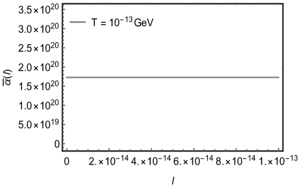
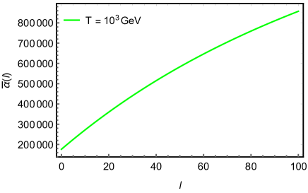
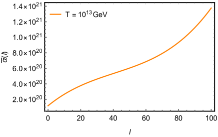
Figure 9: The figure shows the correction to the Stefan–Boltzmann law represented by parameter $\bar{\alpha}$ as a function of $l(\text{whose dimension is}\,\,m\cdot kg^{-1/2}\cdot s^{-1})$ considering the temperatures of cosmic microwave background (top left), electroweak scenario (top right), and the early inflationary universe (bottom).

$$\bar{F}(\beta,l)=\frac{1}{\pi^{2}\beta}\int^{\infty}_{0}\left(\frac{E^{2}+lE^{3}}{1-lE}\right)^{1/2}\left[\frac{(2E+3lE^{2})(1-lE)+l(E^{2}+lE^{3})}{(1-lE)^{2}}\right]\,\mathrm{ln}\left(1-e^{-\beta E}\right)\mathrm{d}E,$$ (26)

$$\begin{split}\bar{S}(\beta,l)=\frac{k_{B}}{\pi^{2}}&\int_{0}^{\infty}\left\{-\left(\frac{E^{2}+lE^{3}}{1-lE}\right)^{1/2}\left[\frac{(2E+3lE^{2})(1-lE)+l(E^{2}+lE^{3})}{(1-lE)^{2}}\right]\,\mathrm{ln}\left(1-e^{-\beta E}\right)\right.\\ &\left.+E\left(\frac{E^{2}+lE^{3}}{1-lE}\right)^{1/2}\left[\frac{(2E+3lE^{2})(1-lE)+l(E^{2}+lE^{3})}{(1-lE)^{2}}\right]\frac{\,e^{-\beta E}}{1-e^{-\beta E}}\right\}\mathrm{d}E,\end{split}$$

$$\bar{C}_{V}(\beta,l) = \frac{k_{B}\beta^{2}}{\pi^{2}}\int_{0}^{\infty}dE\times$$

$$\times \left\{E^{2}\left(\frac{E^{2}+lE^{3}}{1-lE}\right)^{1/2}\left[\frac{(2E+3lE^{2})(1-lE)+l(E^{2}+lE^{3})}{(1-lE)^{2}}\right]\frac{e^{-2\beta E}}{\left(1-e^{-\beta E}\right)^{2}}\right.$$

$$+ \left.E^{2}\left(\frac{E^{2}+lE^{3}}{1-lE}\right)^{1/2}\left[\frac{(2E+3lE^{2})(1-lE)+l(E^{2}+lE^{3})}{(1-lE)^{2}}\right]\frac{e^{-\beta E}}{1-e^{-\beta E}}\right\}.$$

Initially, we provide the analysis of the Helmholtz free energy displayed in Eq. (26); it is considered within three different scenarios of the Universe: CMB, primordial electroweak epoch, and inflationary era. All these results are demonstrated in Fig. 10, which displays a trivial contribution to the first case, and a decreasing characteristic for the latter two ones. Next, we examined the entropy which was shown in Eq. (III); we investigated such thermal function in the same different scenarios of the Universe. All these considerations were shown in Fig. 11, which exhibited the same trivial contribution to the first case, despite of showing an increase characteristic to the latter two ones. Finally, we studied the heat capacity exhibited in Eq. (III); we also examined this thermal function in the same different scenarios of the Universe. All these considerations were shown in Fig. 12, exhibiting a trivial contribution to the first case as well, and increasing curves for the next two ones.

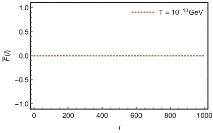
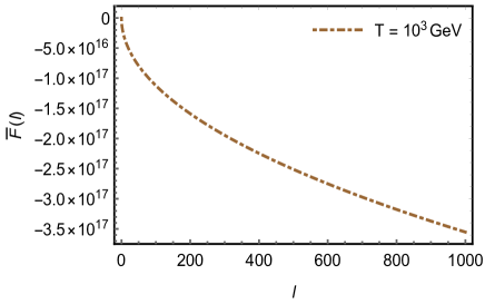
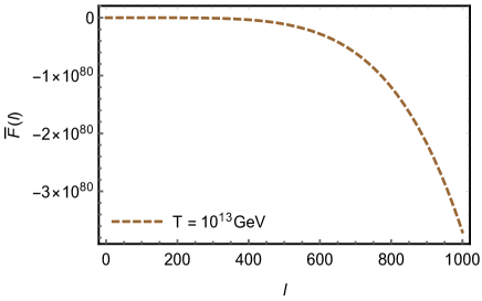
Figure 10: The figure shows the modification of the Helmholtz free energy $\bar{F}$ as a function of $l(\text{whose dimension is}\,\,m\cdot kg^{-1/2}\cdot s^{-1})$ considering the temperatures of cosmic microwave background (top left), electroweak scenario (top right), and the early inflationary universe (bottom).

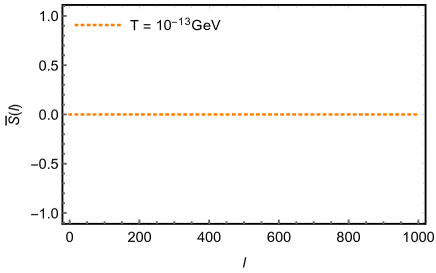
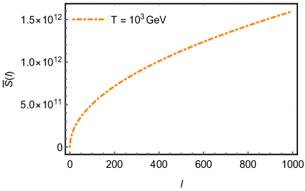
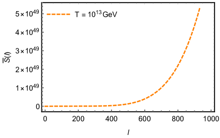
Figure 11: The figure shows the modification of the entropy $\bar{S}$ as a function of $l(\text{whose dimension is}\,\,m\cdot kg^{-1/2}\cdot s^{-1})$ considering the temperatures of cosmic microwave background (top left), electroweak scenario (top right) and the early inflationary universe (bottom).

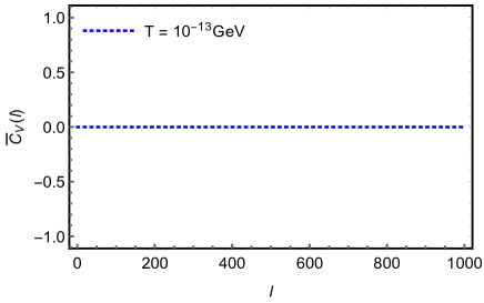
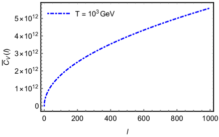
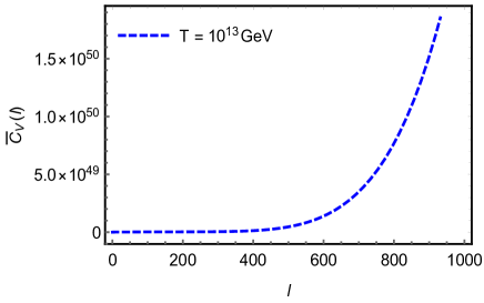
Figure 12: The figure shows the modification of the heat capacity $\bar{C}_{V}$ as a function of $l(\text{whose dimension is}\,\,m\cdot kg^{-1/2}\cdot s^{-1})$ considering the temperatures of cosmic microwave background (top left), electroweak scenario (top right) and the early inflationary universe (bottom).

Here, just as we did in the previous section, we also present the analysis of the equation of state. Moreover, since there is no analytical solution to perform our analysis, we have to consider a particular limit to obtain its magnitude as we did before. The limit that we study is $(E^{2}+lE^{3})^{1/2}/(1-lE)^{2}\ll 1$. With it, we obtain the following expression

$$p=\frac{1}{45\pi^{2}}T^{6}\left[270l^{2}\zeta(5)+4\pi^{4}\frac{l}{T}+90\frac{1}{T^{2}}\zeta(3)\right].$$ (28)

The behavior of Eq. (28) is displayed in Fig 13. Differently with what happens to the model involving $\sigma$, the dispersion relation coming from Eq. (18) has a fascinating feature: the shape exhibited to the equation of states turns out to be sensitive to the modification of the values of $l$. Furthermore, note that, if we consider $l\rightarrow 0$, we obtain

$$p=\frac{90\zeta(3)}{45\pi^{2}}T^{4}.$$ (29)

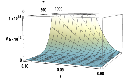
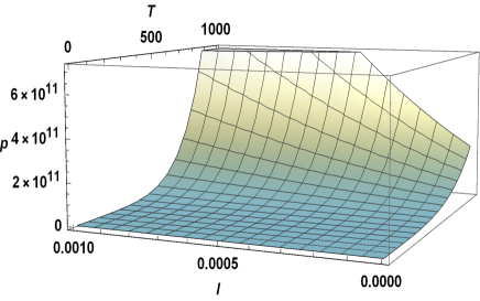
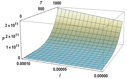
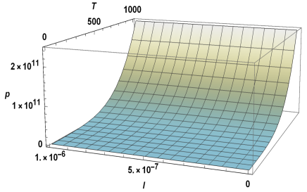
Figure 13: The figure shows the equation of states for different values of $p$, $T$, and $l(\text{whose dimension is}\,\,m\cdot kg^{-1/2}\cdot s^{-1})$.

IV Conclusion

We considered the thermodynamical aspects of two higher-derivative Lorentz-breaking theories, namely, CPT-even and CPT-odd ones. Within our study, we focused on the dispersion relations rather than the specific form of the Lagrangians. In this way, we expect that our results can be applied not only to scalar field models as we assumed, but also to specific gauge or spinor field theories.

We calculated the modification to the black body radiation spectra and to the Stefan–Boltzmann law due to the parameters $\sigma$ and $l$. For these theories, we explicitly obtained the corresponding equation of states and the thermodynamic functions as well, i.e., the mean energy, the Helmholtz free energy, the entropy, and the heat capacity. Moreover, all the calculations presented in this work were performed taking into account three different scenarios of the Universe: cosmic microwave background, electroweak epoch, and inflationary era.

Furthermore, since the heat capacity rapidly increased with the Lorentz-breaking parameters at high temperatures, perhaps one might expect a phase transition in those scenarios. Nevertheless, a further investigation in this direction might be accomplished in order to provide a proper examination. Thereby, as a further perspective, we suggest the detailed study of the whole field of Horava-Lifshitz gravity model and the possible phase transitions in our models. Another feasible continuation of this study can consist in its application to other higher-derivative Lagrangians of certain known field theories, f.e. those ones discussed in mariz2019quantum .

References

• (1) S. Liberati and L. Maccione, “Astrophysical constraints on planck scale dissipative phenomena,” Physical Review Letters, vol. 112, no. 15, p. 151301, 2014.
• (2) J. D. Tasson, “What do we know about lorentz invariance?,” Reports on Progress in Physics, vol. 77, no. 6, p. 062901, 2014.
• (3) A. Hees, Q. G. Bailey, A. Bourgoin, P.-L. Bars, C. Guerlin, L. Poncin-Lafitte, et al., “Tests of lorentz symmetry in the gravitational sector,” Universe, vol. 2, no. 4, p. 30, 2016.
• (4) R. Maluf, A. Araújo Filho, W. Cruz, and C. Almeida, “Antisymmetric tensor propagator with spontaneous lorentz violation,” EPL (Europhysics Letters), vol. 124, no. 6, p. 61001, 2019.
• (5) J. Alfaro, H. A. Morales-Tecotl, and L. F. Urrutia, “Loop quantum gravity and light propagation,” Physical Review D, vol. 65, no. 10, p. 103509, 2002.
• (6) M. Pospelov and Y. Shang, “Lorentz violation in hořava-lifshitz-type theories,” Physical Review D, vol. 85, no. 10, p. 105001, 2012.
• (7) N. E. Mavromatos, “Lorentz invariance violation from string theory,” arXiv preprint arXiv:0708.2250, 2007.
• (8) S. M. Carroll, J. A. Harvey, V. A. Kosteleckỳ, C. D. Lane, and T. Okamoto, “Noncommutative field theory and lorentz violation,” Physical Review Letters, vol. 87, no. 14, p. 141601, 2001.
• (9) V. A. Kosteleckỳ and N. Russell, “Data tables for lorentz and c p t violation,” Reviews of Modern Physics, vol. 83, no. 1, p. 11, 2011.
• (10) J. Collins, A. Perez, D. Sudarsky, L. Urrutia, and H. Vucetich, “Lorentz invariance and quantum gravity: an additional fine-tuning problem?,” Physical Review Letters, vol. 93, no. 19, p. 191301, 2004.
• (11) J. Nascimento, A. Y. Petrov, and C. M. Reyes, “Renormalization in a lorentz-violating model and higher-order operators,” The European Physical Journal C, vol. 78, no. 7, pp. 7, 578, 2018.
• (12) R. C. Myers and M. Pospelov, “Ultraviolet modifications of dispersion relations in effective field theory,” Physical Review Letters, vol. 90, no. 21, p. 211601, 2003.
• (13) V. A. Kosteleckỳ and M. Mewes, “Electrodynamics with lorentz-violating operators of arbitrary dimension,” Physical Review D, vol. 80, no. 1, p. 015020, 2009.
• (14) V. A. Kosteleckỳ and Z. Li, “Gauge field theories with lorentz-violating operators of arbitrary dimension,” Physical Review D, vol. 99, no. 5, p. 056016, 2019.
• (15) T. Mariz, J. Nascimento, A. Y. Petrov, and C. M. Reyes, “Quantum aspects of the higher-derivative lorentz-breaking extension of qed,” Physical Review D, vol. 99, no. 9, p. 096012, 2019.
• (16) D. Colladay and P. McDonald, “Statistical mechanics and lorentz violation,” Physical Review D, vol. 70, no. 12, p. 125007, 2004.
• (17) R. Casana, M. M. Ferreira Jr, and J. S. Rodrigues, “Lorentz-violating contributions of the carroll-field-jackiw model to the cmb anisotropy,” Physical Review D, vol. 78, no. 12, p. 125013, 2008.
• (18) R. Casana, M. M. Ferreira Jr, J. S. Rodrigues, and M. R. Silva, “Finite temperature behavior of the c p t-even and parity-even electrodynamics of the standard model extension,” Physical Review D, vol. 80, no. 8, p. 085026, 2009.
• (19) M. Gomes, T. Mariz, J. Nascimento, A. Petrov, A. Santos, and A. da Silva, “Free energy of lorentz-violating qed at high temperature,” Physical Review D, vol. 81, no. 4, p. 045013, 2010.
• (20) A. Araújo Filho, “Lorentz-violating scenarios in a thermal reservoir,” The European Physical Journal Plus, vol. 136, no. 4, pp. 1–14, 2021.
• (21) A. Araújo Filho and R. Maluf, “Thermodynamic properties in higher-derivative electrodynamics,” Brazilian Journal of Physics, vol. 51, no. 3, pp. 820–830, 2021.
• (22) A. Araújo Filho and J. Reis, “Thermal aspects of interacting quantum gases in lorentz-violating scenarios,” The European Physical Journal Plus, vol. 136, no. 3, pp. 1–30, 2021.
• (23) M. Anacleto, F. Brito, E. Maciel, A. Mohammadi, E. Passos, W. Santos, and J. Santos, “Lorentz-violating dimension-five operator contribution to the black body radiation,” Physics Letters B, vol. 785, pp. 191–196, 2018.
• (24) S. Das, S. Ghosh, and D. Roychowdhury, “Relativistic thermodynamics with an invariant energy scale,” Physical Review D, vol. 80, no. 12, p. 125036, 2009.
• (25) A. Y. Petrov et al., “Bouncing universe in a heat bath,” arXiv preprint arXiv:2105.05116, 2021.
• (26) J. Reis, S. Ghosh, et al., “Fermions on a torus knot,” arXiv preprint arXiv:2108.07336, 2021.
• (27) G. Amelino-Camelia, “Testable scenario for relativity with minimum length,” Physics Letters B, vol. 510, no. 1-4, pp. 255–263, 2001.
• (28) S. Bianco, V. N. Friedhoff, and E. Wilson-Ewing, “Modified dispersion relations, inflation, and scale invariance,” Physical Review D, vol. 97, no. 4, p. 046006, 2018.
• (29) M. Gomes, F. Marques, T. Mariz, J. Nascimento, A. Y. Petrov, and A. da Silva, “One-loop corrections in the z= 3 lifshitz extension of qed,” Physical Review D, vol. 98, no. 10, p. 105016, 2018.
• (30) P. Horava, “Quantum Gravity at a Lifshitz Point,” Phys. Rev. D, vol. 79, p. 084008, 2009.
• (31) K. de Farias, T. Sampaio, M. Anacleto, F. Brito, and E. Passos, “Lifshitz-scaling in CPT-even Lorentz-violating electrodynamics and GRB time delay,” Eur. Phys. J. Plus, vol. 136, no. 2, p. 257, 2021.
• (32) F. Reif, “Fundamentals of statistical and thermal physics,” 1998.
• (33) J. W. Gibbs, Elementary principles in statistical mechanics. Courier Corporation, 2014.
• (34) W. Greiner, L. Neise, and H. Stöcker, Thermodynamics and statistical mechanics. Springer Science & Business Media, 2012.
• (35) H. B. Callen, “Thermodynamics and an introduction to thermostatistics,” 1998.
• (36) R. Maluf, D. Dantas, and C. Almeida, “The casimir effect for the scalar and elko fields in a lifshitz-like field theory,” The European Physical Journal C, vol. 80, pp. 1–10, 2020.
• (37) N. Zettili, “Quantum mechanics: concepts and applications,” 2003.
• (38) R. R. Oliveira, A. A. Araújo Filho, F. C. Lima, R. V. Maluf, and C. A. Almeida, “Thermodynamic properties of an aharonov-bohm quantum ring,” The European Physical Journal Plus, vol. 134, no. 10, p. 495, 2019.
• (39) R. Oliveira and A. Araújo Filho, “Thermodynamic properties of neutral dirac particles in the presence of an electromagnetic field,” The European Physical Journal Plus, vol. 135, no. 1, p. 99, 2020.
• (40) J. Reis et al., “How does geometry affect quantum gases?,” arXiv preprint arXiv:2012.13613, 2020.
• (41) I. Lobo, V. Bezerra, J. M. Graça, L. C. Santos, and M. Ronco, “Effects of planck-scale-modified dispersion relations on the thermodynamics of charged black holes,” Physical Review D, vol. 101, no. 8, p. 084004, 2020.
• (42) I. Lobo and G. Santos, “Thermal dimensional reduction and black hole evaporation,” arXiv preprint arXiv:2009.08556, 2020.
• (43) G. Amelino-Camelia, F. Brighenti, G. Gubitosi, and G. Santos, “Thermal dimension of quantum spacetime,” Physics Letters B, vol. 767, pp. 48–52, 2017.
• (44) G. Rosati, G. Amelino-Camelia, A. Marciano, and M. Matassa, “Planck-scale-modified dispersion relations in frw spacetime,” Physical Review D, vol. 92, no. 12, p. 124042, 2015.
• (45) G. Amelino-Camelia, L. Barcaroli, G. D’Amico, N. Loret, and G. Rosati, “Icecube and grb neutrinos propagating in quantum spacetime,” Physics Letters B, vol. 761, pp. 318–325, 2016.
• (46) G. Amelino-Camelia, G. D’Amico, G. Rosati, and N. Loret, “In vacuo dispersion features for gamma-ray-burst neutrinos and photons,” Nature Astronomy, vol. 1, no. 7, pp. 1–6, 2017.