Variety of scaling laws for DNA thermal denaturation

Abstract

We discuss possible mechanisms that may impact the order of the transition between denaturated and bound DNA states and lead to changes in the scaling laws that govern conformational properties of DNA strands. To this end, we re-consider the Poland-Scheraga model and apply a polymer field theory approach to calculate entropic exponents associated with the denaturated loop distribution. We discuss in particular variants of this transition that may occur due to the properties of the solution and may affect the self- and mutual interaction of both single and double strands. We find that the effects studied significantly influence the strength of the first order transition. This is manifest in particular by the changes in the scaling laws that govern DNA loop and strand distribution. As a quantitative measure of these changes we present the values of corresponding scaling exponents. For the $d=4-\varepsilon$ case we get corresponding $\varepsilon^{4}$ expansions and evaluate the perturbation theory expansions at space dimension $d=3$ by means of resummation technique.

1 Introduction

In its native state DNA has a form of a helix that consists of two strands bound together by hydrogen bonds. During biological processes involving DNA (such as duplication or transcription) unbinding occurs, phenomenon known also as denaturation, helix-to-coil transition or DNA unzipping [1, 2, 3]. An analogue to DNA unwinding in a cell can be observed also in vitro, in solutions of purified DNA. Already in the middle 50-ies of the last century it has been observed that heating of DNA solutions above room temperature results in cooperative transition of the bound helix-structures strands to single strands. Although the mechanism of such unwinding clearly differs from the biological protein-mediated process, ongoing experimental studies of DNA alone are important steps toward understanding much more complex phenomenon that occurs in vivo in a cell [4]. The mechanism of such transition may be an external pulling force applied to one of DNA strands (mechanical unzipping), changes in the pH of the DNA contained solvent (chemical unzipping) or its heating (thermal unzipping) [1]. The scaling laws that govern this last phenomenon are the subject of analysis in our paper. It is our great honour to submit this paper to the Physica A special issue in memoriam of Dietrich Stauffer: his contribution to statistical physics in general and to studies of scaling properties of many-agent interacting systems is hard to be overestimated.

One of important experimental observations of the DNA melting curves, where the fraction of the bound pairs $\theta(T)$ is measured as a function of temperature $T$ is their abrupt behaviour [1, 5]. With an increase of $T$, $\theta(T)$ manifests a jump at certain transition temperature clearly signaling that the DNA thermal denaturation is a first order transition. Numerous theoretical approaches to represent the process of DNA thermal denaturation in a two-state Ising-like manner were developed. Here, we concentrate on the Poland-Scheraga type description, where the transition is governed by an interplay of two factors: chain binding energy and configurational entropy [2, 3, 6]. In turn, the entropy of the macromolecule in a good solvent attains a scaling form and this is how the scaling exponents that govern configurational properties of polymer macromolecules of different topology [7, 8] come into play in descriptions of DNA thermal denaturation [9, 10, 11, 12].

Similar as the Ising model suggested to describe ferromagnetism fails if one models a ferromagnet as a 1d chain [13], the Poland-Scheraga model suggested to describe the 1st order transition of DNA thermal denaturation fails (predicting the 2nd order scenario) if one models DNA strands as non-interacting random walks (RWs) [2, 3]. With a span of time (see a short overview in the next section) it became clear that an account of in- and inter-strand interactions plays crucial role and leads to correct picture of the transition. In particular the role of interactions between denaturated DNA loop and bound chain has been analyzed both numerically [14, 11] and analytically [9, 10]. Corresponding analytical calculations have been performed by field-theoretic approach in $d=4-\varepsilon$ dimensions with $\varepsilon^{2}$ accuracy [10]. Besides, it was suggested [11] that chain heterogeneity may impact the order of the transition too.

So far, the origin of such heterogeneity has been attributed to effective scaling behaviour differing from that of a self-avoiding walk (SAW). However, it is well known that depending on temperature, the asymptotic scaling behaviour of a flexible macromolecule belongs either to RW ($T=T_{\theta}$) or to SAW ($T>T_{\theta}$) universality class ($T_{\theta}$ denoting the $\theta$-point) [15]. Therefore, it is tempting to recast the heterogeneity in scaling behaviour of a single- and double-stranded chains by studying asymptotic scaling properties of mutually interacting SAWs and RWs. This is the main goal of our paper. To this end, we apply a polymer field theory to calculate entropic exponents associated with the denaturated loop distribution. Doing so, besides calculating a set of new scaling exponents that govern DNA loop and strand distribution for heterogeneous chains we also get higher precision values of the familiar exponents that have been calculated for the homogeneous case [10]. The set-up of the paper is as follows: in the next section 2 we give a short history of Poland-Scheraga model and discuss the polymer network description for DNA denaturation. There we obtain scaling relations that enable quantitative analysis of the order of DNA thermal denaturation transition in terms of co-polymer star exponents. We obtain perturbation theory expansions for the scaling exponents and evaluate them in 3d case in section 3. Conclusions and outlook are given in section 4.

2 Poland-Scheraga model and polymer network description for DNA denaturation

One of the first models to explain the DNA denaturation as the first order transition was coined in middle-sixties by Poland and Scheraga [2, 3]. Two observations lay at the core of the model: (i) the breaking of hydrogen bonds between nucleobases is an energy-demanding process, therefore the low-$T$ bound state is energetically favoured, and (ii) a high-$T$ unbound state has more configurations and hence it is favoured by entropy. Being simple enough to allow analytic and numerical treatments and at the same time capturing main peculiarities of the phenomena involved, the model gave rise to a whole direction of studies, see e.g. [6, 5, 9, 10, 11, 12, 14, 16, 17, 18, 19].

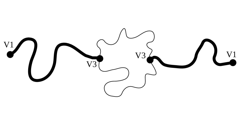
Figure 1: Model of DNA thermal denaturation we consider in this study. A double stranded macromolecule with end points $V1$ is disattached (‘unzipped’) at points $V3$. Resulting heterogeneous polymer network consists of two double strands $V1-V3$ (bound nucleobases, bold lines) and a denaturated single-stranded loop $V3-V3$ (unbound nucleobases, thin lines). Partition function of the loop attains a power-law scaling (1).

The Poland-Scheraga description, relies on a representation of the partition function ${\cal Z}$ of a polymer of $N$ segments, each segment being in two possible states (bound and unbound monomers, see Fig. 1) in a form ${\cal Z}=x_{1}^{N}$, $x_{1}$ being maximal solution of the equation suggested in [20]. In turn, this allows to get the order parameter $\theta(T)$ (average number of ordered, bound pairs in a chain) and to observe different regimes for its temperature $T$ dependence. These regimes are triggered by the loop closure exponent $c$ for a single loop, defined as

$${\cal Z}_{\rm loop}\sim\mu^{\ell}\ell^{-c},$$ (1)

where $\ell$ is loop length (number of segments) and $\mu$ is a non-universal factor. In particular, for low values of $c$, $0\leq c\leq 1$ the order parameter is continuous function of $T$ smoothly changing between 0 and 1 when $T$ decreases from $\infty$ to 0. For larger values of $c$ the order parameter either continuously vanishes at $T=T_{c}$ for $1<c\leq 2$ or disappears abruptly at $T=T_{c}$ for $c>2$. The last two types of behaviour correspond to the second and first order phase transitions.

First attempts to define exponent $c$ analytically let to $1<c<2$ and hence to the second order transition scenario. In particular, for a simplified model which considers a single denaturated loop and does not take into account interaction between bound and unbound segments (non-interacting RWs) one may obtain $c$ by enumerating walks that return to the origin leading to $c=1$, $c=3/2$ for $d=2$, $d=3$, correspondingly [3]. A more general formula $c=d\nu$, with $\nu$ being polymer end-to-end distance scaling exponent was coined by Fisher [16]. In particular, it allows to take into account excluded volume effects for each of the segments. Its prediction is $c(d=2)=3/2$, $c(d=3)\simeq 1.764$ and hence the transition still remains the second order. An interaction of a loop with the rest of the chain was taken into account in [9, 10] by making use of polymer network scaling description [7, 8]. There, the configurational properties of a homogeneous SAW polymer network with a single denaturated loop were recast in terms of the corresponding scaling exponents. The phase transition was found to be of the first order for $d=2$ and above, with $c(d=2)=2+13/32\simeq 2.41$, $c(d=3)\simeq 2.115$. Numerical simulations at $d=3$ further supported the first order scenario with $c(d=3)=2.10(4)$ [14] and $c(d=3)=2.18)6)$ [11]. Effect of possible heterogeneity was partially taken into account in [11] by assuming that entropic scaling exponents may differ for different parts of the network and introducing fit parameters to quantify such difference.

Let us find the exponent $c$, Eq. (1) that governs scaling of a denaturated loop in the simplified picture of DNA unzipping considering that the macromolecule consists of chains of two different species, as shown in Fig. 1. The loop is formed by unbound nucleobases, let us take it to be of ‘species 1’ whereas the two chains $V1-V3$, $V3-V1$ consist of bound nucleobases, ‘species 2’. In order to evaluate entropy of a single loop in a network in Fig. 1, we will make use of scaling picture for copolymer networks, as suggested in [21, 22]. In particular, the partition function (number of configurations) of a copolymer nework ${\cal G}$ made of $F_{1}$ chains of species 1 and $F_{2}$ chains of species 2 scales with a mean size of a single polymer chain $R$ as [21]:

$${\cal Z_{G}}\sim R^{\eta_{\cal G}-F_{1}\eta_{2,0}-F_{2}\eta_{0,2}},$$ (2)

with

$$\eta_{\cal G}=-d{\cal L}+\sum_{f_{1}+f_{2}\geq 1}n_{f_{1},f_{2}}\eta_{f_{1},f_{2}},$$ (3)

where $d$ is space dimension, ${\cal L}$ is the number of loops in the network, $n_{f_{1},f_{2}}$ is number of vertices where $f_{1}$ chains of species 1 and $f_{2}$ chains of species 2 meet. Exponents $\eta_{f_{1}f_{2}}$ constitute a family of copolymer star exponents [21]. Each of them describes scaling of a copolymer star of corresponding functionality, made of $f_{1}$ chains of species 1 and $f_{2}$ chains of species 2. Being universal, they depend only on space dimension $d$ and the number of chains $f_{1}$, $f_{2}$, as well as three different types of fixed points (FPs) that govern scaling behavior [15]. These FPs correspond to the cases when (i) both species 1 and 2 are mutually interacting SAWs, the so-called symmetric fixed point $S$, (ii) species 1 and 2 are mutually interacting SAWs and RWs, correspondingly, unsymmetric fixed point $U$ and (iii) both species 1 and 2 are RWs, however there is mutual avoidance interaction between species 1 and 2, fixed point $G$. By case (i) one recovers the homogeneous polymer network, whereas cases (ii) and (iii) present non-trivial examples of copolymer scaling. Therefore the scaling properties of a heterogeneous polymer network made of interacting SAWs and RWs can be reformulated in terms scaling exponents of co-polymer stars made of two interacting sets of SAWs ($\eta^{S}_{f_{1}f_{2}}$), of RWs ($\eta^{G}_{f_{1}f_{2}}$) or of a set of SAWs that interacts with RWs ($\eta^{U}_{f_{1}f_{2}}$) [24]. Field-theoretical renormalization group calculations of the above copolymer star exponents resulted in $\varepsilon=4-d$ expansions which have been obtained successively within $\varepsilon^{3}$ [21] and $\varepsilon^{4}$ [23] accuracy.

According to the above, one can distinguish four different cases that take into account heterogeneity of the network shown in Fig. 1 and consider mutual avoidance between all SAWs and RWs. In each of this cases, applying Eq. (3) we arrive at the following expressions for $\eta_{\cal G}$:

• SAW-SAW-SAW: both chains $V_{1}-V_{3}$ and $V_{3}-V_{3}$ are SAWs,

  $$\eta_{\cal G}=-d+2\eta^{S}_{12}$$ (4)

• SAW-RW-SAW: chains $V_{1}-V_{3}$ are SAWs, chains $V_{3}-V_{3}$ are RWs;

  $$\eta_{\cal G}=-d+2\eta^{U}_{12}$$ (5)

• RW-SAW-RW: chains $V_{1}-V_{3}$ are RWs, chains $V_{3}-V_{3}$ are SAWs;

  $$\eta_{\cal G}=-d+2\eta^{U}_{21}$$ (6)

• RW-RW-RW: all chains $V_{1}-V_{3}$ and $V_{3}-V_{3}$ are RWs.

  $$\eta_{\cal G}=-d+2\eta^{G}_{12}$$ (7)

In the ’symmetric’ case (i) we recover usual homogeneous polymer picture by taking into account that $\eta^{S}_{12}=\eta_{3}$, $\eta_{3}$ being scaling exponent of the homogeneous three-leg SAW star [7, 8].

With the above expressions for the heterogeneous co-polymer network exponents $\eta_{\cal G}$ at hand, it is straightforward to proceed deriving loop closure exponents for each of the cases (i)-(iv). To this end, following [9, 12] we generalize expression (2) to the case when the network is formed by chains of different sizes: $R$ for the side chains $V1-V3$ and $r$ for the loop $V3-V3$. Then the expression for the partition function reads:

$${\cal Z_{G}}\sim R^{\eta_{\cal G}-F_{1}\eta^{U}_{20}}f(r/R).$$ (8)

Here $f(x)$ is the scaling function, $F_{1}$ is the number of SAWs in the network and we have taken into account that the exponent $\eta^{U}_{02}=0$ for RWs [24]. Furthermore, considering the limit $r/R\to 0$ we apply the short-chain expansion [25] and make use of the observation that for vanishing loop size the partition function (8) should reduce to that of a single (either SAW or RW) chain, ${\cal Z}_{\rm chain}\sim R^{\eta_{\rm chain}}$ with $\eta_{\rm chain}=\eta^{U}_{02}=0$ for RW and $\eta_{\rm chain}=\eta^{U}_{20}$ for SAW [24]. This implies the power-law asymptotics for the scaling function:

$$f(x)\sim x^{y},\hskip 10.00002pt{\rm with}\hskip 10.00002pty=\eta_{\cal G}-F_{1}\eta^{U}_{20}-\eta_{\rm chain}\,.$$ (9)

Indeed, with (9) the partition function factorizes as

$${\cal Z_{G}}\sim R^{\eta_{\rm chain}}\times r^{y}\sim{\cal Z}_{\rm chain}{\cal Z}_{\rm loop}\,.$$ (10)

Comparing Eqs. (1) and (9) one arrives at the following expression for the loop closure exponent $c$:

$$c=\nu_{\rm loop}[\eta_{\rm chain}-\eta_{\cal G}+F_{1}\eta^{U}_{20}]\,,$$ (11)

where $\nu_{\rm loop}$ is the end-to-end distance scaling exponent of the loop forming chain, ${\cal Z}_{\rm loop}\sim r^{y}\sim\ell^{\nu_{\rm loop}y}$.

Combining formula (11) with the corresponding expressions for $\eta_{\cal G}$ of four different heterogeneous networks formed by mutually interacting SAWs and RWs, Eqs. (4)–(7) we arrive at the following loop closure exponents in each of these networks, in the following denoted as $c_{1}$–$c_{4}$:

SAW-SAW-SAW: $$c_{1}=\nu_{\rm SAW}(3\eta^{S}_{20}+d-2\eta^{S}_{12})\,,$$ (12)

SAW-RW-SAW: $$c_{2}=\nu_{\rm RW}(\eta^{S}_{20}+d-2\eta^{U}_{12})\,,$$ (13)

RW-SAW-RW: $$c_{3}=\nu_{\rm SAW}(2\eta^{S}_{20}+d-2\eta^{U}_{21})\,.$$ (14)

RW-RW-RW: $$c_{4}=\nu_{\rm RW}(d-2\eta^{G}_{21})\,,$$ (15)

where $\nu_{\rm RW}=1/2$ and $\nu_{\rm SAW}$ are the end-to-end mean distance exponents for RW and SAW, correspondingly. By (1), each of the above expressions govern the loop closure in the heterogeneous network and therefore defines the order of the phase transition of DNA thermal denaturation in the frames of the Poland-Scheraga model. In the following section we will evaluate these expressions for the case $d=3$.

3 $\varepsilon$-expansion and its resummation

Scaling relations (12)–(15) express exponents $c_{i}$ in terms of the familiar co-polymer star exponents $\eta_{f_{1}f_{2}}$ [21]. The latter have been calculated by means of field-theoretic renormalization group approach and are currently available in $\varepsilon=4-d$-expansion up to order $\varepsilon^{4}$ [23]. Completing these expansions by familiar $\varepsilon$-expansion for the exponent $\nu_{\rm SAW}$, see e.g. [26], one readily gets the corresponding expansions for exponents $c_{i}$:

$$c_{1}=2+1/8\,\varepsilon+{\frac{5}{256}}\,{\varepsilon}^{2}+\left(-{\frac{87}{4096}}+{\frac{3}{512}}\,\zeta\left(3\right)\right){\varepsilon}^{3}+$$

$$\left(-{\frac{3547}{262144}}+{\frac{903}{16384}}\,\zeta\left(3\right)+{\frac{1}{20480}}\,{\pi}^{4}-{\frac{1815}{2048}}\,\zeta\left(5\right)\right){\varepsilon}^{4},$$ (16)

$$c_{2} = 2+1/8\,\varepsilon+\left({\frac{17}{256}}-{\frac{21}{64}}\,\zeta\left(3\right)\right){\varepsilon}^{2}+$$ (17)

$$\left(-{\frac{63}{512}}\,\zeta\left(3\right)-{\frac{39}{4096}}\right){\varepsilon}^{3}+\Big{(}-{\frac{3015}{262144}}+$$

$${\frac{105}{16384}}\,\zeta\left(3\right)+{\frac{1185}{2048}}\,\zeta\left(5\right)-{\frac{21}{20480}}\,{\pi}^{4}\Big{)}{\varepsilon}^{4},$$

$$c_{3} = 2+3/4\,\varepsilon+\left({\frac{21}{128}}-{\frac{21}{32}}\,\zeta\left(3\right)\right){\varepsilon}^{2}+$$ (18)

$$\left({\frac{157}{2048}}-{\frac{27}{128}}\,\zeta\left(3\right)\right){\varepsilon}^{3}+\Big{(}{\frac{4125}{131072}}-{\frac{165}{1024}}\,\zeta\left(3\right)-$$

$${\frac{11}{10240}}\,{\pi}^{4}-{\frac{465}{1024}}\,\zeta\left(5\right)\Big{)}{\varepsilon}^{4},$$

$$c_{4}=2+1/2\,\varepsilon\,,$$ (19)

where $\zeta(x)$ is Riemann $\zeta$-function. Note that because of $\eta^{G}_{21}=\eta^{G}_{12}=-1$ [21] the corresponding analytic expression for $c_{4}$ is exact and contains only linear term.

Perturbative renormalization group expansions have zero radius of convergence and are asymptotic at best [26, 27]. Special resummation procedures are used to restore their convergence and to get reliable numerical estimates on their basis. Below we will make use of the Borel resummation refined by conformal mapping [28] which is known to be a powerful tool in analysis of $\varepsilon$-expansions. In general, the method is applied to the function in form of a series expansion:

$$\upsilon(x)=\sum\limits_{n=0}c_{n}x^{n},$$ (20)

with known asymptotics of the coefficients $c_{n}$:

$$\lim_{n\to\infty}c_{n}\sim n!(-a)^{n}\,.$$ (21)

The Borel sum associated with (20) is used to mitigate the factorial growth of the expansion coefficients

$$B(x)=\sum\limits_{n=0}\frac{c_{n}x^{n}}{n!}\,.$$ (22)

The resulting series is supposed to converge, in the complex $x$-plane, inside a circle of radius $1/a$ (cf. Eq. (21), where $x=-1/a$ is the singularity of $B(x)$ closest to the origin. Then using the definition of the $\Gamma$-function one can rewrite Eq. (20) as

$$\upsilon(x)=\sum\limits_{n=0}\frac{c_{n}x^{n}}{n!}\int_{0}^{\infty}dt\,e^{-t}t^{n}\,.$$ (23)

Interchanging summation and integration in Eq. (23) leads to the definition of the Borel transform of $\upsilon(x)$ as

$$\upsilon_{B}(x)=\int_{0}^{\infty}dt\,e^{-t}\upsilon(xt)\,.$$ (24)

In order to perform the integral in (24) on the whole real positive semiaxis, one has to find an analytic continuation of $B(x)$. To this end, assuming that singularities in $B(x)$ lie on the negative semiaxis with the singularity closest to the origin located at $1/a$, and that the function $B(x)$ is analytical in the complex plane excluding the part of real axis $(-\infty;-\frac{1}{a})$, one passes to new variables $\omega$ conformally mapping the cut plane onto a disk of radius 1:

$$x=\frac{4}{a}\frac{\omega}{(1-\omega)^{2}}$$ (25)

The procedure is further refined by introducing two additional fit parameters $b$ and $\alpha$. The first one is introduced substituting the factorial $n!$ in Eq. (21) by the Euler gamma-function $\Gamma(n+b+1)$ and inserting an additional factor $t^{b}$ into the integral (23). The fit parameter $\alpha$ is introduced to weaken the singularity by multiplying the expression under the integral by $(1-\omega)^{\alpha}$. The expression for the resummed function reads:

$$\upsilon_{R}(x)=\sum_{n}d_{n}(\alpha,a,b)\int_{0}^{\infty}dt\,t^{b}e^{-t}\frac{\omega^{n}(xt)}{(1-\omega(t)^{\alpha}}\ .$$ (26)

Explicit form of the coefficients $d_{n}(\alpha,a,b)$ is found on the base of known expansion coefficients $c_{n}$ in Eq. (20). In practice, procedure (26) is applied to the truncated series (20), which is known up to order $L$. Let us denote the value of the resummed truncated function at given fixed $x$ by $\upsilon_{R}^{(L)}$. Ideally, such value (that usually corresponds to certain physical observable) should not depend on resummation parameters $\alpha$ and $b$. To eliminate such dependence, for each perturbation theory order $L$ one choses optimal values of $\alpha_{opt}^{(L)},b_{opt}^{(L)}$ which satisfy condition of minimal sensitivity [29]:

$$\frac{\partial\upsilon_{R}^{(L)}(b,\alpha)}{\partial b}\arrowvert_{b_{opt}^{(L)},\alpha_{opt}^{(L)}}=\frac{\partial\upsilon_{R}^{(L)}(b,\alpha)}{\partial\alpha}\arrowvert_{b_{opt}^{(L)},\alpha_{opt}^{(L)}}=0\,.$$ (27)

In this way, a set of optimal values $(b,\alpha)^{L}$ is obtained for every perturbation theory order $L$. Out of these points one has to choose those that ensure the fastest converge by minimizing values:

$$\upsilon_{R}^{(L+1)}(b^{(L+1)},\alpha^{(L+1)})-\upsilon_{R}^{(L)}(b^{(L)},\alpha^{(L)})\,.$$ (28)

The above described procedure has been applied to obtain the results discussed below. As we have checked by explicit calculations, the resummation method described above does not lead to consistent results when directly applied to series (16)–(18) at $\varepsilon=1$. This may serve as an evidence of their Borel-nonsummability. Another obvious way to get numerical estimates of the exponents $c_{i}$ is to resum series for the exponents that enter right-hand sides of scaling relations (12)–(14) and then use these relations to evaluate $c_{i}$. The resummed values of exponents $\nu$, $\eta_{f_{1}f_{2}}$ are given in Table 1 at $d=3$ in different orders of perturbation theory. As one can see from the Table, the resummation restores convergence of the $\varepsilon$-expansion for the exponents and leads to reliable numerical estimates. As a benchmark one can use the state-of-the art estimate for the $\nu_{\rm SAW}$ exponent obtained via conformal bootstrap $\nu_{\rm SAW}(d=3)=0.5877(12)$ [30] and MC simulations $\nu_{\rm SAW}(d=3)=0.5875970(4)$ [31] which reasonably well compare with our result $0.585(3)$ as given in the Table. Note that $\varepsilon$-expansion for the $\nu_{\rm SAW}$ exponent is currently available with a record $\varepsilon^{7}$ accuracy and the most recent hypergeometric-Meijer resummation of this series lead to an estimate $\nu_{\rm SAW}(d=3)=0.58770(17)$ [32].

	$I$	$II$	$III$	$IV$
$\nu_{SAW}$	0.54(3)	0.56(2)	0.582(8)	0.585(3)
$\eta^{S}_{20}$	-0.25(6)	-0.292(4)	-0.289 (5)	-0.276(3)
$\eta^{S}_{12}$	-0.75(4)	-0.77(2)	-0.75(1)	-0.743(5)
$\eta^{U}_{12}$	-0.75(8)	-0.82(5)	-0.77(3)	-0.795(5)
$\eta^{U}_{21}$	-1.(2)	-0.9(8)	-0.95(8)	-0.98(3)

Table 1: Scaling exponents $\nu$, $\eta_{f_{1}f_{2}}$ obtained at $d=3$ by resummation of $\varepsilon$-expansion in different orders of perturbation theory.

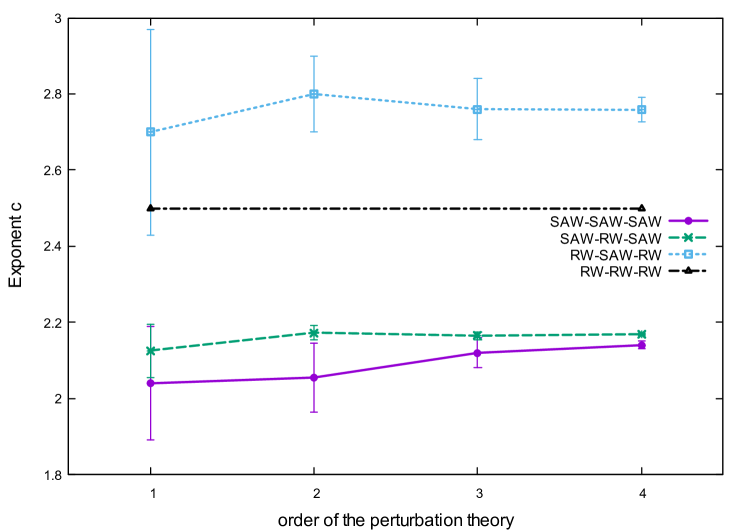
Figure 2: Loop closure exponents $c_{i}$ of the heterogeneous co-polymer network of interacting SAWs and RWs (as shown in Fig. 1) in different orders of the perturbation theory.

	$I$	$II$	$III$	$IV$
$c_{1}$ (SAW-SAW-SAW)	2.04 (15)	2.05 (9)	2.12 (4)	2.147 (9)
$c_{2}$ (SAW-RW-SAW)	2.12 (7)	2.17 (2)	2.16 (1)	2.169 (4)
$c_{3}$ (RW-SAW-RW)	2.7 (3)	2.8 (1)	2.76 (8)	2.76 (3)
$c_{4}$ (RW-RW-RW)	2.5	2.5	2.5	2.5

Table 2: Loop closure exponents $c_{i}$ (12)–(15) in different orders of perturbation theory for different combinations of interacting SAWs and RWs.

Using numerical estimates for the exponents $\nu$, $\eta_{f_{1}f_{2}}$ one can evaluate loop closure exponents $c_{i}$ in successive orders of the $\varepsilon$-expansion. The results are given in Table 2 and further displayed in Fig. 2. One observes that the numbers nicely converge with an increase of the perturbation theory order and thus provide reliable numerical estimates for the loop closure exponent in the case of heterogeneus co-polymer network. These results will be further discussed in the next section.

4 Conclusions

Influence of possible heterogeneity in entropic scaling exponents of bound and denaturated DNA strands on the loop closure exponent $c$ is manifest by an interplay of two factors. On the one hand, the number of configurations of a denaturated loop, cf. Fig. 1, is influenced by the loop self-avoidance interactions (the number is larger for the RW loop and smaller of the SAW one). On the other hand, the number of loop configurations is restricted by the side chains. Calculations presented here give a reliable way to judge about the values of exponents $c_{i}$ for different heterogeneity conditions and hence to judge about the order of DNA thermal denaturation transition. Our analysis is grounded on the field theory of co-polymer networks [21, 22]. By scaling relations (12)–(15) we connect loop closure exponents $c_{i}$ to scaling exponents $\eta_{f1f2}$ that govern entropic properties of co-polymer stars made by mutually interacting sets of SAWs and RWs. Using powerful resummation technique, we resum $\varepsilon^{4}$ expansions for these exponents and evaluate them at space dimension $d=3$. Numerical results for the exponents $c_{i}$ are listed in Table 2 and shown in Fig. 2. As one can see, the effects of heterogeneity significantly influence the strength of the first order transition (the exponent $c$ increases in comparison to the usual homogeneous SAW case).

Details of our calculations together with analysis of the 2d case will be a subject of a separate publication [33]. We acknowledge useful discussions with Maxym Dudka and Ralph Kenna. This work was supported in part by the National Academy of Sciences of Ukraine, project KPKBK 6541230.

References

- [1] R.M. Wartell, A.S. Benight, Phys. Rep. 126(2) (1985) 67.
- [2] D. Poland, H.A. Scheraga, J. Chem. Phys 45 (1966) 1456.
- [3] D. Poland, H.A. Scheraga, J. Chem. Phys. 45 (1966) 1464.
- [4] R.D. Blake et al., Bioinformatics 15 (1999) 370; R. Blossey, E. Carlon, Phys.Rev. E 68 (2003) 061911.
- [5] M. Reiter-Schad, E. Werner, J. Tegenfeldt, B. Mehlig, T. Ambjörnsson. J. Chem. Phys. 143 (2015) 115101.
- [6] D. Poland, H.A. Scheraga. Theory of Helix-Coil Transitions in Biopolymers: Statistical Mechanical Theory of Order-Disorder Transitions in Biological Macromolecules, Academic Press, Inc. (1970)
- [7] B. Duplantier, Phys. Rev. Lett. 57 (1986) 941; B. Duplantier, J. Stat. Phys. 54 (1989) 581.
- [8] L. Schaäfer, C. von Ferber, U. Lehr, B. Duplantier, Nucl. Phys. B 374 (1992) 473.
- [9] Y. Kafri, D. Mukamel, L. Peliti, Phys. Rev. Lett. 85 (2000) 4988.
- [10] Y. Kafri, D. Mukamel, L. Peliti, Eur. Phys. J B 27 (2002) 135.
- [11] M. Baiesi, E. Carlon, A.L. Stella, Phys. Rev. E 66 (2002) 021804.
- [12] E. Carlon, M. Baiesi, Phys. Rev. E 70 (2004) 066118.
- [13] E. Ising, Z. Physik 31 (1925) 253; T. Ising, R. Folk, R. Kenna, B. Berche, Yu. Holovatch, J. Phys. Stud. 21 (2017) 4001.
- [14] E. Carlon, E. Orlandini, A. L. Stella, Phys. Rev. Lett. 88 (2002) 198101.
- [15] L. Schäfer, C. Kapeller, J. Phys. (Paris) 46 (1985) 1853 (1985); Colloid Polym. Sci. 268 (1990) 995; L. Schäfer, U. Lehr, C. Kapeller, J. Phys. I1 (1991) 211.
- [16] M. Fisher, J. Chem. Phys. 45 (1966) 1469.
- [17] C. Richard, A. Guttmann, J. Stat. Phys. 115 (2004) 925.
- [18] Q. Berger, G. Giacomin, M. Khatib, Annales Henri Lebesgue 3 (2020) 299.
- [19] A. Legrand, Electron. J. Probab. 26 (2021), article no. 10, 1-43.
- [20] S. Lifson, J. Chem. Phys. 40 (1964) 3705.
- [21] C. von Ferber, Yu. Holovatch, Phys. Rev. E 56 (1997) 6370; C. von Ferber, Yu. Holovatch, Europhys. Lett. 39 (1997) 31.
- [22] C. von Ferber, Yu. Holovatch, Phys. Rev. E 59 (1999) 6914.
- [23] V. Schulte-Frohlinde, Yu. Holovatch, C. von Ferber, A. Blumen, Phys. Lett. A 328 (2004) 335.
- [24] When in the unsymmetrical fixed point , the first index in counts number of SAWs, the second one counts number of RWs.
- [25] C. von Ferber, Nucl. Phys. B 490 (1997) 511.
- [26] H.Kleinert, V.Schulte-Frohlinde. Critical Properties of -Theories. World Scientific, Singapore, 2001.
- [27] J. Zinn-Justin. Quantum Field Theory and Critical Phenomena, 3rd ed., Oxford University Press, New York, 1989.
- [28] J.C. Le Guillou, J. Zinn-Justin, Phys. Rev. B 21 (1980) 3976.
- [29] B. Delamotte, Yu. Holovatch, D. Ivaneyko, D. Mouhanna, M. Tissier, J. Stat. Mech. (2008) 03014; B. Delamotte, M. Dudka, Yu. Holovatch, D. Mouhanna, Phys. Rev. B 82 (2010) 104432.
- [30] H. Shimada, S. Hikami, J. Stat. Phys. 165 (2016) 1006.
- [31] N. Clisby, B. Dunweg, Phys. Rev. E 94 (2016) 052102.
- [32] A. M. Shalaby, preprint arXiv:2005.12714 (2020).
- [33] Yu. Honchar, C. von Ferber, Yu. Holovatch, in preparation (2021)