To $H_{0}$ or not to $H_{0}$?

Abstract

This paper investigates whether changes to late time physics can resolve the ‘Hubble tension’. It is argued that many of the claims in the literature favouring such solutions are caused by a misunderstanding of how distance ladder measurements actually work and, in particular, by the inappropriate use of a distance ladder $H_{0}$ prior. A dynamics-free inverse distance ladder shows that changes to late time physics are strongly constrained observationally and cannot resolve the discrepancy between the SH0ES data and the base $\Lambda$CDM cosmology inferred from Planck. We propose a statistically rigorous scheme to replace the use of $H_{0}$ priors.

1 Introduction

As is well known, a six parameter $\Lambda$CDM cosmology has proved to be spectacularly successful in explaining the cosmic microwave background radiation (CMB), light element abundances and a wide range of other astronomical data (e.g. Planck Collaboration et al., 2018; Efstathiou & Gratton, 2019; Mossa et al., 2020; eBOSS Collaboration et al., 2020). As noted in Planck Collaboration et al. (2018), the agreement between the base $\Lambda$CDM model and observations is so good, that many researchers have begun to focus on possible discrepancies or ‘tensions’, with the hope that the model might break to reveal new truths about our Universe. This is reasonable given that many ingredients of the model, particularly the physics describing the dark sector, remain mysterious at this time.

The discrepancy between early time and late time determinations of the Hubble constant, $H_{0}$, is probably the most serious such tension. This tension became apparent following the first results from the Planck satellite (Planck Collaboration et al., 2014) which revealed a discrepancy between the best fit base $\Lambda$CDM value of $H_{0}$ and the Cepheid-based distance ladder measurement of $H_{0}$ by the SH0ES collaboration (Riess et al., 2011). Since then, the ‘Hubble tension’ (as it has become known) has intensified: recent results from the SH0ES collaboration give $H_{0}=74.03\pm 1.42~{}\text{km}~{}\text{s}^{-1}\text{Mpc}^{-1}$ (Riess et al., 2019, hereafter R19) (udpating the results of Riess et al. (2016), hereafter R16) which differs by $4.3\sigma$ from the base $\Lambda$CDM value $H_{0}=67.44\pm 0.58~{}\text{km}~{}\text{s}^{-1}\text{Mpc}^{-1}$ inferred from the most recent analysis of Planck (Efstathiou & Gratton, 2019). To add to the conundrum, the lower value of $H_{0}$ inferred from the CMB is in very good agreement with various applications of an inverse distance ladder, irrespective of whether the sound horizon, $r_{d}$, is fixed to a value determined from the CMB or to a value inferred from primordial nucleosynthesis (e.g. Aubourg et al., 2015; Verde et al., 2017; Addison et al., 2018; Abbott et al., 2018; Macaulay et al., 2019).

Possible modifications to the base $\Lambda$CDM model that might resolve this tension have been discussed in the reviews by Knox & Millea (2020), Beenakker & Venhoek (2021) and Di Valentino et al. (2021). In broad brush, the proposed solutions fall into four categories: (i) radical departures from conventional cosmology, including departures from General Relativity; (ii) changes to the physics of the early Universe (for example adding additional relativistic species, or neutrino interactions); (iii) new physics at matter-radiation equality, or recombination, that alters the value of the sound horizon, (iv) changes to the expansion history at late times. The focus of this paper is on solutions in class (iv).

The issue of whether the tension is real is not yet fully clear (see Freedman et al., 2019; Yuan et al., 2019; Freedman et al., 2020). Despite the fact that the author is an unashamed Hubble tension skeptic (Efstathiou, 2020), I will take the SH0ES results at face value in this paper and consider whether the Hubble tension can be resolved by modifications to the $\Lambda$CDM  late time expansion history.

Figure 1 shows various measurements of $H(z)$ from baryon acoustic oscillation (BAO) experiments. The normalization of these measurements assumes the Planck value of the sound horizon

$$r_{d}=147.31\pm 0.31\ \text{Mpc}.$$ (1)

Throughout this paper we will assume that the base $\Lambda$CDM model describes accurately the physics at early times and so $r_{d}$ is fixed to Eq. (1). The sources for the observational data points are listed in the figure caption. The green line shows $H(z)$ for the best fit base $\Lambda$CDM cosmology determined from Planck and the grey bands show $1\sigma$ and $2\sigma$ ranges. The green line approaches the value $H_{0}^{P}=67.44~{}\text{km}~{}\text{s}^{-1}\text{Mpc}^{-1}$ asymptotically as $z\rightarrow 0$. As long as $r_{d}$ remains fixed, apparently the only way to reconcile the BAO data with the SH0ES value of $H_{0}$ is to modify the base $\Lambda$CDM curve. For example, the dashed line in Fig. 1 shows the relation

$$H(z) = H^{f}_{0}\bigg{[}\Omega_{m}(1+z)^{3}+\qquad\qquad\qquad\qquad$$ (2)

$$\qquad(1-\Omega_{m})\left(1+\Delta\exp(-(z/z_{c})^{\beta})\right)\bigg{]}^{1/2},\qquad$$

with parameters $H^{f}_{0}=H^{P}_{0}$, $\Omega_{m}=0.31$, $\Delta=0.30$, $z_{c}=0.1$ and $\beta=2$. With this choice of parameters, the value of $H_{0}$ matches the SH0ES value whilst matching the BAO $H(z)$ measurements at $z>0.3$.

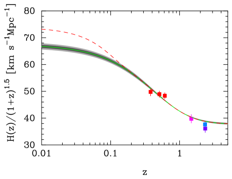
Figure 1: The evolution of the Hubble parameter with redshift. The red points  show $H(z)$ measurements in three redshift bins inferred from galaxy correlations in the Baryon Oscillation Spectroscopic Survey (BOSS) Alam et al. (2017). The purple point at $z=2.35$ shows $H(z)$ from BAO features in the cross-correlations of Ly$\alpha$ absorbers and quasars (Blomqvist et al., 2019). The blue point at $z=2.34$ shows $H(z)$ from BAO features in the correlations of Ly$\alpha$ absorbers (de Sainte Agathe et al., 2019). The magenta point at $z=1.48$ shows $H(z)$ from BAO feaures in the correlations of quasars (Hou et al., 2020). The green line shows $H(z)$ for the best-fit base $\Lambda$CDM determined from Planck and the grey bands show $1\sigma$ and $2\sigma$ ranges. The dashed line shows Eq. (2) with parameters chosen to match the SH0ES value of $H_{0}$ at $z=0$.

If the dashed curve is interpreted as a variation in the equation of state of the dark energy, then it necessarily requires a phantom equation of state, $w<-1$, at low redshifts. Alternatively, one might imagine that transference of energy between the dark matter and dark energy results in something like the dashed curve. Models of both types have been proposed as ‘solutions’ to the Hubble tension as summarized in Di Valentino et al. (2021). These ‘solutions’ are not viable because the SH0ES team does not directly measure $H_{0}$.

In fact, the SH0ES team measure the absolute peak magnitude, $M_{B}$, of Type Ia supernovae (SN), assumed to be standard candles, by calibrating the distances of SN host galaxies to local geometric distance anchors via the Cepheid period luminosity relation. The magnitude $M_{B}$ is then converted into a value of $H_{0}$ via the magnitude-redshift relation of the Pantheon SN sample (Scolnic et al., 2017) of supernovae in the redshift range $0.023<z<0.15$. All of the proposed late time ‘solutions’ to the Hubble tension reviewed in Di Valentino et al. (2021) interpret the SH0ES $H_{0}$ measurement as a measurement of the value of $H(z)$ as $z\rightarrow 0$ (often imposing a SH0ES ‘$H_{0}$ prior’) without investigating whether the ‘solution’ is consistent with the magnitude-redshift relation of Type Ia SN. It is hardly advancing our understanding if authors propose solutions to the $H_{0}$ tension that are inconsistent with the measurements that they are trying to explain.

This point was first made by Lemos et al. (2019) and more recently by Benevento et al. (2020) and by Camarena & Marra (2021), but has been comprehensively ignored in recent literature. The purpose of this paper is to show how theoretical models exploring new physics at late time should be compared with distance ladder measurements, avoiding the use of a SH0ES $H_{0}$ prior. I will adopt a ‘dynamics free’ approach to this problem and show that late time modifications of the $\Lambda$CDM expansion history cannot resolve the Hubble tension.

2 The Inverse Distance Ladder

We will write the metric of space-time as

$$ds^{2}=c^{2}dt^{2}-R^{2}(t)(dx^{2}+dy^{2}+dz^{2}),$$ (3)

adopting a spatially flat geometry consistent with the very tight experimental constraints on spatial curvature (Efstathiou & Gratton, 2020). The Hubble parameter, $H=R^{-1}dR/dt$, then fixes the luminosity distance $D_{L}(z)$ and comoving angular diameter distance $D_{M}(z)$ according to

$$D_{L}(z)=c(1+z)\int_{0}^{z}{dz^{\prime}\over H(z^{\prime})},\\ \quad D_{M}(z)={D_{L}(z)\over(1+z)}.$$ (4)

Standard candles and standard rulers can therefore be used to constrain $H(z)$ independently of any dynamics (Heavens et al., 2014; Bernal et al., 2016; Lemos et al., 2019; Aylor et al., 2019) . As long as the relations of Eq. (4) are satisfied, it does not matter whether modifications to the functional form of $H(z)$ are caused by by changes to the equation of state of dark energy or interactions between dark matter and dark energy.

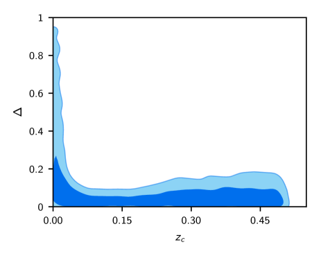
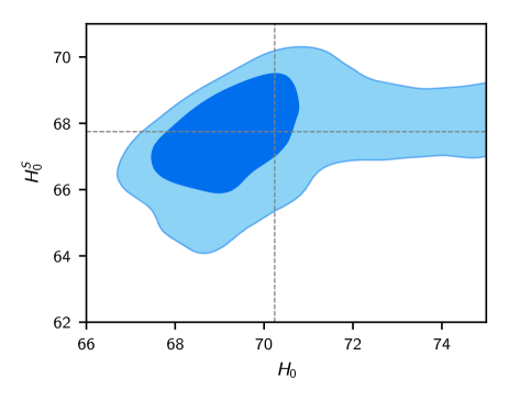
Figure 2: 68 and 95% constraints on the parameters $\Delta$ and $z_{c}$ (left hand panel) and the SH0ES-like parameter $H^{S}_{0}$ of Eq. (10b) and $H_{0}$. (right hand panel). The dashed lines in the right hand panel show the best fit values of $H^{S}_{0}$ and $H_{0}$.

A standard candle with absolute magnitude $M$ at redshift $z$ will have an apparent magnitude

$$m = M+25+5\log_{10}D_{L}(z),$$ (5a)

$$= -5a+5\log_{10}c\hat{d}_{L}(z)$$ (5b)

with $D_{L}$ in units of Mpc. In (5b), $a$ is the intercept of the magnitude-redshift relation, $5a=-(M+25-5\log_{10}H_{0})$ and $\hat{d}_{L}(z)=H_{0}D_{L}(z)/c$. The SH0ES Cepheid data allow one to calibrate the absolute magnitude $M_{B}$ of Type Ia SN. Combining the geometrical distance estimates of the maser galaxy NGC 4258 (Reid et al., 2019), detached eclipsing binaries in the Large Magellanic Cloud (Pietrzyński et al., 2019) and GAIA early data release 3 (EDR3, Lindegren et al. (2020a, b)) parallax measurements of 75 Milky Way Cepheids with HST photometry as reported in Riess et al. (2021) (hereafter R21), the SH0ES Cepheid photometry and Pantheon SN peak magnitudes give

$$M_{B}=-19.214\pm\ 0.037\ {\rm mag.}$$ (6)

(see Sect. 3). To estimate $H_{0}$, R16 determine the intercept of the Pantheon SN magnitude-redshift relation by fitting the low redshift expansion to the luminosity distance

$$\hat{d}_{l}(z)=z\left[1+(1-q_{0}){z\over 2}-{1\over 6}(1-q_{0}-3q_{0}^{2}+j_{0})z^{2}\right],$$ (7)

over the redshift range $z=0.023$ to $z=0.15$, with the deceleration and jerk parameters set to $q_{0}=-0.55$ and $j_{0}=1$ (close to the values for base $\Lambda$CDM, $q_{0}=-0.535$, $j_{0}=1$). They find

$$a_{B}=0.71273\pm 0.00176,$$ (8)

which, together with Eq. (6), gives

$$H_{0}=74.1\pm 1.3~{}\text{km}~{}\text{s}^{-1}\text{Mpc}^{-1},$$ (9)

(see Table 2). This is slightly higher than the value $H_{0}=73.2\pm 1.3~{}\text{km}~{}\text{s}^{-1}\text{Mpc}^{-1}$ quoted in R21 reflecting differences in the period ranges and photometric samples used in my analysis. These differences are unimportant for this paper. (Note, however, that the global fits to the SH0ES Cepheid data using the GAIA EDR3 parallaxes have puzzling features as discussed in Sect. 3.)

To apply the inverse distance ladder, I follow closely the analysis described in Lemos et al. (2019). $H(z)$ is parameterized by Eq. (2) and the parameters of the model are determined by fitting to Pantheon SN magnitudes and the BAO $D_{M}(z)$ and $H(z)$ measurements from the references given in the caption to Fig. 1, supplemented by the $D_{V}(z)=(D_{M}^{2}(z)cz/H(z))^{1/3}$ measurement at $z=0.106$ from Beutler et al. (2011). The free parameters of the model are $H_{0}^{f}$, $\Omega_{m}$, $\Delta$, $z_{c}$, $\beta$ and $M_{B}$ with uniform priors as listed in Table 1. To compare with the BAO results, I adopt a Gaussian prior on the sound horizon $r_{d}$ with the parameters of Eq. (1). I use the MULTINEST sampling algorithm (Feroz et al., 2009, 2011) to explore the parameter space.

Table 1: Results of applying the inverse distance ladder. The table lists the mean values of the parameters and their $1\sigma$ error. The last column lists the ranges over which a uniform prior is applied to the parameters. The parameters $H_{0}$ and $H^{S}_{0}$ are derived parameters (see Eqs. 2 and 10b). The units of $H^{f}_{0}$, $H_{0}$ and $H^{S}_{0}$ are $~{}\text{km}~{}\text{s}^{-1}\text{Mpc}^{-1}$.

parameter	fit	prior range
$H^{f}_{0}$	$68.13\pm 1.00$	$60\ \textendash\ 80$
$\Omega_{m}$	$0.306\pm 0.017$	$0.25\ \textendash\ 0.35$
$\Delta$	$0.107\pm 0.162$	$0.0\ \textendash\ 1.0$
$z_{c}$	$0.167\pm 0.091$	$0.001\ \textendash\ 0.5$
$\beta$	$2.45\pm 0.86$	$1.0\ \textendash\ 4.0$
$M_{B}$	$-19.387\pm 0.021$	$-19.0\ \textendash\ -19.5$
$H_{0}$	$70.5\pm 3.6$	–
$H^{S}_{0}$	$67.73\pm 0.97$	–

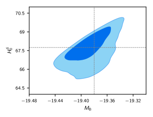
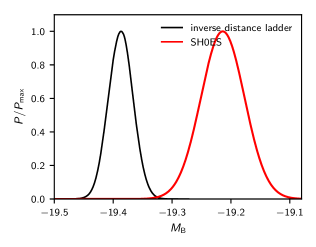
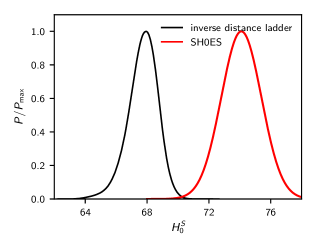
Figure 3: The left hand panel shows 68 and 95% constraints on the parameters $H_{0}^{S}$ and $M_{B}$. The dotted lines show the mean values of these parameters listed in Table 1. The midle panel shows the marginalised posterior distributions of the SN peak absolute magnitude $M_{B}$ determined from the inverse distance ladder discussed in this paper (black line) compared with the posterior distribution of $M_{B}$ determined from the SH0ES data (red line). The right hand panel shows the equivalent plot, but for the parameter $H^{S}_{0}$ instead of $M_{B}$.

The constraints on these parameters are summarized in Table 1. The left hand plot in Fig. 2 shows the $1\sigma$ and $2\sigma$ constraints on the parameters $\Delta$ and $z_{c}$. The key point here is that the parameter $\Delta$ is well constrained for values of $z_{c}\lower 2.15277pt\hbox{$\;\buildrel>\over{\sim}\;$}0.05$ because at these redshifts the form of $H(z)$ is tightly constrained by the SN magnitude-redshift relation. At lower values of $z_{c}$, the parameter $\Delta$ becomes poorly constrained by the SN magnitude-redshift relation and solutions with high values of $H_{0}$ are allowed. This reinforces the conclusions of Benevento et al. (2020) and Camarena & Marra (2021) that the SN data are insensitive to changes in the dark energy equation of state at very late times.

We can compute a derived quantity $H^{S}_{0}$ that is equivalent to the SH0ES estimate of $H_{0}$

$$a_{B} = \left(\sum_{ij}C^{-1}_{ij}(\log_{10}\hat{d}_{L}(z)-0.2m_{B}(i))\right)/\sum_{ij}C^{-1}_{ij}\qquad\qquad$$ (10a)

$$H^{S}_{0} = 10^{0.2(M_{B}+5a_{B}+25)}$$ (10b)

where $$C 0.023-0.15$$ is the covariance matrix of the Pantheon SN magnitudes and the sums in Eq. (10a) extend all SN in the Pantheon sample with redshifts in the range .

The right hand plot in Fig. 2 shows $H^{S}_{0}$ plotted against the true value of $H_{0}$. One can see the long tail extending to high values of $H_{0}$. These high values arise in solutions with $z_{c}\lower 2.15277pt\hbox{$\;\buildrel<\over{\sim}\;$}0.05$ and high values of $\Delta$ corresponding to phantom-like equations of state. However, the SH0ES analysis is oblivious to these high values of $H_{0}$. Instead, a SH0ES type analysis would infer a value close to the estimate $H^{S}_{0}$ of Eq. (10b), which is always low. For these models $H^{S}_{0}=67.75\pm 1.01~{}\text{km}~{}\text{s}^{-1}\text{Mpc}^{-1}$, discrepant with Eq. (9) by $3.9\sigma$ despite the ability of the model to mimic extreme phantom-like equations of state. It is also worth noting that the parameters $\Omega_{m}$ and $H_{0}^{S}$ are each within about $0.4\sigma$ of the base $\Lambda$CDM values inferred from Planck. There is not even a hint from these data for any phantom-like physics.

The discrepancy between the inverse distance ladder and the SH0ES data is illustrated clearly in Fig. 3. The left hand panel shows the $1\sigma$ and $2\sigma$ constraints on $H^{S}_{0}$ and $M_{B}$. The central panel shows the posterior distribution of $M_{B}$ determined from the inverse distance ladder (black line) compared with the result of Eq. (7) derived from the SH0ES data (red line). The right hand panel shows the posterior distribution of $H^{S}_{0}$ compared with Eq. (9). The SH0ES results are clearly discrepant with the inverse distance ladder. As long as the Planck value of $r_{d}$ is correct and the relations of Eq. (4) apply, modifications to the expansion history at late times cannot explain the SH0ES data.

3 Should one use a SH0ES $H_{0}$ prior?

The first draft of this paper generated a large number of comments. Many of the negative comments cited the paper by Dhawan et al. (2020) which explored a number of parametric forms for the expansion history (interpreted as modifications to the dark energy equation of state) constrained to fit the Pantheon magnitude-redshift relation. Dhawan et al. (2020) concluded that the distance ladder values of $H_{0}$ inferred for these expansion histories agreed to within about $0.5~{}\text{km}~{}\text{s}^{-1}\text{Mpc}^{-1}$ (excluding models with a sharp transition in the equation of state at very low redshift, which were not considered by Dhawan et al. (2020)). Critics of my paper have argued that the insensitivity of $H_{0}$ to variations in the expansion history found by Dhawan et al. (2020) means that it is safe to use a SH0ES $H_{0}$ prior in cosmological parameter analysis even if the Pantheon sample is excluded from the analysis. This is incorrect.

The key point is that the Pantheon SN sample is an essential part of the SH0ES distance ladder measurement of $H_{0}$. Summarising the entire SH0ES analysis in terms of one parameter, namely the value of $H_{0}$, represents a huge and lossy compression of the Cepheid+SN data. In particular, all information on the shape of the SN magnitude-redshift relation is lost. If one then imposes a SH0ES $H_{0}$ prior but ignores the Pantheon SN data, it is possible to infer evidence for phantom like dark energy as illustrated by the dotted line in Fig. 1. However, such a solution is strongly disfavoured by the Pantheon magnitude-redshift relation.

If one wants to investigate consequences of new late-time physics, a rigorous way of compare with the SH0ES results, as noted by Camarena & Marra (2021), is to drop $H_{0}$ as a parameter in favour of the SN peak absolute magnitude $M_{B}$. In other words, rather than explaining the ‘Hubble tension’ one should instead focus on the ‘supernova absolute magnitude tension’ since this is what the Cepheid calibrations are designed to measure. The goal then is to find a late time solution that brings $M_{B}$ measured from distant supernovae into agreement with the value inferred from Cepheid measurements. This necessarily involves analysing a uniformly calibrated supernova sample such as Pantheon. The following procedure is statistically rigorous:

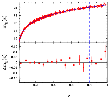
Figure 4: The upper panel shows the magnitude-redshift relation for the Pantheon sample, together with the best fit (solid line) assuming the expansion history of Eq. (12). The vertical dashed line shows the maximum redshift used in the fit. The lower panel shows maximum likelihood band averaged residuals with respect to the best fit, together with $1\sigma$ errors.

[1] If correlations between the host galaxy SN magnitudes and the magnitudes of more distant supernovae are ignored (as in the the SH0ES papers and this paper) the SH0ES Cepheid measurements can be summarized by the posterior distribution of the SN peak absolute magnitude $M^{1}_{B}$. If one wants to take into account correlations between the magnitudes of host and distant SN, the SH0ES data must be summarized in terms of a vector of distance moduli ${\boldsymbol{\mu}}$ and an associated covariance matrix as described in Appendix A.

[2] To test a theoretical model, carry as parameters an absolute magnitude $M^{1}_{B}$ for the Cepheid SN host galaxies and an absolute magnitude $M^{2}_{B}$ for the more distant SN in the Pantheon sample (taking into account correlations with the Cepheid SN magnitudes, if necessary). If the posteriors of $M^{1}_{B}$ and $M^{2}_{B}$ overlap, then one has a candidate solution to the ‘supernova absolute magnitude tension’.

[3] If there is substantial overlap between the posteriors of $M^{1}_{B}$ and $M^{2}_{B}$, one can replace these parameters by a single parameter $M_{B}$. The best fit value of $M_{B}$ for a chosen cosmology is equivalent to a best fit value of $H_{0}$.

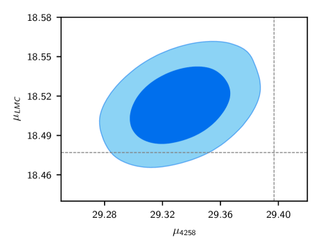
Figure 5: 68% and 95% constraints on the NGC 4258 and LMC distance moduli for the three anchor global fit summarized in column 5 of Table 2. The best fit geometrical distance moduli of (Reid et al., 2019) and (Pietrzyński et al., 2019) (which are included as priors in the global fit) are shown by the dotted lines.

Table 2: Determination of $H_{0}$ from three geometrical distance anchors (NGC 4258 maser distance, LMC detached eclipsing binaries and GAIA DR3 parallaxes to Milky Way Cepheids) using different fits to the expansion history. Column 2 gives results assuming a Gaussian prior on $a_{B}$ of $0.71273\pm 0.00176$ as in R16 and subsequent SH0ES papers. Columns 3 and 4 give results of fitting the $q_{0},j_{0}$ expansion history of Eq. (7) to the Pantheon sample for SN in the redshift range $0.023$ to $z_{\rm max}$. Column 5 shows the results of fitting Eq. (12) to the Pantheon sample over the redshift range $0.023-0.8$. The accuracy of the best fit to the Pantheon magnitude-redshift relation in this case is illustrated in Fig. 4. The units of the parameter $zp$ is $\mu$arcsec and $H_{0}$ is in units of $~{}\text{km}~{}\text{s}^{-1}\text{Mpc}^{-1}$.

parameter	$a_{B}$ prior	Eq. (7) ($z_{\rm max}=0.50$)	Eq. (7) ($z_{\rm max}=0.80$)	Eq. (12) ($z_{\rm max}=0.80$)
$M^{W}_{H}$	$-5.922\pm 0.017$	$-5.922\pm 0.017$	$-5.922\pm 0.017$	$-5.922\pm 0.017$
$b$	$-3.24\pm 0.02$	$-3.24\pm 0.02$	$-3.24\pm 0.02$	$-3.24\pm 0.02$
$Z_{w}$	$-0.22\pm 0.06$	$-0.22\pm 0.05$	$-0.22\pm 0.05$	$-0.22\pm 0.06$
$zp$	$-17.1\pm 4.8$	$-17.2\pm 4.7$	$-17.1\pm 4.7$	$-16.8\pm 4.8$
$M_{B}$	$-19.214\pm 0.037$	$-19.213\pm 0.036$	$-19.212\pm 0.037$	$-19.209\pm 0.037$
$a_{B}$	$0.71273\pm 0.00176$	$0.7174\pm 0.0028$	$0.7164\pm 0.0026$	$0.7162\pm 0.0033$
$H_{0}$	$74.1\pm 1.3$	$75.0\pm 1.3$	$74.8\pm 1.3$	$74.9\pm 1.4$

In the above procedure, there is no danger of reaching erroneous conclusions on late time physics through the innapproprate use of an $H_{0}$ prior. In addition, the Pantheon data is only used only once in testing a particular theoretical model (c.f. Camarena & Marra, 2021). Furthermore, this approach remains valid for models in which the expansion history changes at $z\lower 2.15277pt\hbox{$\;\buildrel<\over{\sim}\;$}0.05$.

What procedure should forward distance ladder measurements follow in reporting a value for $H_{0}$? It is clear that one should fit the expansion history using the Pantheon sample as part of the $H_{0}$ analysis rather than adopting fixed values for $q_{0}$ and $j_{0}$ as in R16. To illustrate this, Table 2 shows results of global fits to the SH0ES Cepheid and Pantheon SN magnitude-redshift relation combining three geometrical distance anchors, as described in Sect. 2. The Cepheid period luminosity is fitted to (see e.g. R21)

$$m^{i}_{j}=\mu_{i}+M^{W}_{H}+b(\log_{10}P_{j}-1)+Z_{w}\Delta[O/H]_{j},$$ (11)

where $m^{i}_{j}$ is the H-band Weisenheit apparent magnitude of Cepheid $j$ in galaxy $i$, $P_{j}$ is the period of Cepheid $j$ in units of days and $\Delta[O/H]_{j}$ is the metallicity assigned to Cepheid $j$ relative to Solar metallicity. As in R21 I include a constant offset $zp$ to the GAIA EDR3 parallaxes as a free parameter. Column 2 shows results assuming the R16 prior on $a_{B}$ (Eq. 8) which gives the value of $H_{0}$ quoted in Eq. (9). The next two columns show results using the ($q_{0}$, $j_{0}$) expansion of Eq. (7) which we fit to the Pantheon magnitude-redshift relation over the redshift ranges $0.023-0.5$ (column 3) and $0.023-0.8$ (column 4). The Cepheid period-luminosity parameters, and the parameter $M_{B}$ are stable across the columns, as expected since these parameters are statistically decoupled from the Pantheon magnitude-redshift relation. However, the value of the Hubble constant increases by $\sim 0.7~{}\text{km}~{}\text{s}^{-1}\text{Mpc}^{-1}$ between columns 2 and 4.

To test the sensitivity of these results to the assumed expansion history, column 5 in Table 2 shows results for the flexible parametric form:

$$H(z)=H_{0}^{f}\left[A(1+z)^{3}+B+Cz+D\ {\rm ln}(1+z)\right]^{1/2},$$ (12)

with $A$, $B$, $C$ and $D$ as free parameters (Lemos et al., 2019). The best fit SN magnitude-redshift relation is shown in Fig. 4. Equation (12) provides a very accurate fit to the Pantheon magnitude-redshift relation and is very close to the relation for the best-fit Planck base $\Lambda$CDM cosmology (as can be seen from Fig. 13 of Planck Collaboration et al. (2018)). For most purposes, it will be sufficient to quote a value of $H_{0}$ based on fits of a flexible fitting function (or a Gaussian process, see e.g. Shafieloo et al. (2012); Joudaki et al. (2018)) to the Pantheon magnitude-redshift relation. However, there remains an uncertainty in this type of forward estimation of $H_{0}$, which is difficult to quantify, if the expansion history deviates from the base $\Lambda$CDM cosmology at redshifts $z\lower 2.15277pt\hbox{$\;\buildrel<\over{\sim}\;$}0.05$ since such models are poorly constrained by the Pantheon sample (cf. Fig. 2).

It is worth mentioning a peculiar aspect of the solutions in Table 2. Efstathiou (2020) pointed out a $\sim 3\sigma$ tension between the NGC 4258 and LMC geometric distance anchors in the global fits using the R16 Cepheids. This tension becomes stronger if we include the GAIA EDR3 Cepheid parallaxes. This is illustrated in Fig. 5, which shows the constraints on the LMC and NGC 4258 distance moduli ($\mu_{\rm LMC}$ and $\mu_{4258}$) derived from the fit in column 5 of Table 2. The GAIA EDR3 and LMC anchors pull the solution towards high values of $H_{0}$, while the NGC 4258 maser anchor wants to pull the solution to lower values of $H_{0}$. The three-anchor solutions listed in Table 2 (and in R21) are therefore statistically inconsistent.

4 Conclusions and Discussion

The Hubble tension has led to a large literature in the last few years. Authors of proposed late time solutions to the Hubble tension have often imposed a SH0ES $H_{0}$ prior on the Hubble parameter at $z=0$, leading to erroneous claims of evidence for phantom dark energy, dark matter-dark energy interactions, or other exotic late-time physics. The review article by Di Valentino et al. (2021) cites many such examples.

If one wants to investigate consequences of new late-time physics, the simplest way to compare with the SH0ES results is to drop $H_{0}$ as a parameter in favour of the SN peak absolute magnitude $M_{B}$, i.e. rather than explaining the ‘Hubble tension’ one should instead focus on the ‘supernova absolute magnitude tension’. The goal then is to find a late time solution that brings $M_{B}$ into agreement with the SH0ES measurement. This necessarily involves analysing the Pantheon SN sample. If one wants to combine the SH0ES data with other astrophysical data to constrain late time physics, then one should impose a SH0ES prior on the parameter $M_{B}$ (or Cepheid calibrated distance moduli of SN host galaxies, see Appendix A) and not on the parameter $H_{0}$.

However, using the Pantheon and BAO data, the inverse distance ladder places very strong constraints on new physics at late times. The results of Table 1 show that the data are in excellent agreement with the base $\Lambda$CDM cosmology determined from Planck. BAO is now a mature field employing analysis techniques that have been tested extensively against simulations. There is no good reason to ignore these measurements. Neither is there a good reason to ignore the Pantheon SN sample, since this is an essential part of the SH0ES distance ladder. It is, therefore, unlikely that changes to the late time expansion history can resolve the ‘Hubble tension’. This conclusion is independent of any dynamics, and independent of perturbations insofar as the Planck value of $r_{d}$ is unaltered.

Data Availability

No new data were generated or analysed in support of this research.

Appendix A Including correlations between Cepheid-calibrated SN magnitudes and magnitudes of more distant SN

We denote the covariance matrix of the SN magnitudes as ${\boldsymbol{M}}$ and the covariance matrix of the host galaxy distance moduli as ${\boldsymbol{C}}$. Let $t$ denote the index of the $N_{H}$ host SN and $q$ denote the index of the $N_{P}$ more distant SN in the Pantheon sample that will link the Cepheid measurements to the Hubble flow. The predicted peak SN magnitude in a host galaxy is

$$m^{P}_{t}=\mu_{t}+M^{1}_{B},$$ (13a)

where $$\mu_{t} t z_{q}$$ is the distance modulus to galaxy . The predicted peak SN magnitude for a distant SN at redshift is

$$m^{P}_{q}=\mu(z_{q})+M^{2}_{B},$$ (13b)

where the distance modulus $\mu(z_{q})$ is fixed by an assumed cosmology and value of $H_{0}$. We would expect $M^{1}_{B}=M^{2}_{B}=M_{B}$ if Type 1a supernovae are standard candles. Let ${\boldsymbol{x}}=({\boldsymbol{m}}-{\boldsymbol{m}^{P}})$, where ${\boldsymbol{m}}$ is the data vector of SN peak magnitudes, and partition the vector ${\boldsymbol{x}}$ as (${\boldsymbol{y}}$, $\boldsymbol{w}$) where ${\boldsymbol{y}}$ describes the hosts and ${\boldsymbol{w}}$ describes the more distant SN. Let us partition the covariance matrix ${\boldsymbol{M}}$ as follows:

$${\boldsymbol{M}}^{-1}=\left(\begin{array}[]{c|c}{\boldsymbol{D}}&{\boldsymbol{E}}\\ \hline\cr{\boldsymbol{E}}^{T}&{\boldsymbol{F}}\end{array}\right),$$ (14)

where ${\boldsymbol{D}}$, ${\boldsymbol{E}}$ and ${\boldsymbol{F}}$ have dimensions $N_{H}\times N_{H}$, $N_{H}\times N_{P}$ an $N_{P}\times N_{P}$ respectively.

If correlations between host and distant SN magnitudes are negligible, the Cepheid analysis is decoupled from the analysis of the distant SN in the Pantheon sample. In this case, the Cepheid analysis can be summarized by the posterior distribution of $M^{1}_{B}$ and the likelihood of the distant SN is

$$-2\ln{\cal L}={\boldsymbol{w}}^{T}{\boldsymbol{F}}{\boldsymbol{w}}.$$ (15)

Given an assumed functional form for $D_{L}(z)$, Eq. (15) can be used to determine a probability distribution for $H_{0}$ given a distribution for $M^{1}_{B}=M^{2}_{B}=M_{B}$ . This is the approximation adopted by the SH0ES team and in the main body of this paper.

To take into account correlations between host and distant SN magnitudes, a more complex procedure is necessary. In this case, the Cepheid analysis can no longer be summarized by the posterior distribution of $M^{1}_{B}$. Instead the Cepheid analysis needs to be summarized in terms of the distance moduli for the SN hosts and a covariance matrix. It is a very good approximation to assume a Gaussian probability distribution

$$-2\ln{\cal L}=({\boldsymbol{\mu}}-{\boldsymbol{\mu}}^{m})^{T}{\boldsymbol{C}}^{-1}({\boldsymbol{\mu}}-{\boldsymbol{\mu}}^{m}),$$ (16)

where ${\boldsymbol{\mu}}^{m}$ are the mean values of the host distance moduli determined from the MCMC chains and ${\boldsymbol{C}}$ is their covariance matrix

There is, however, no need to carry the $N_{H}$ components of ${\boldsymbol{\mu}}$ as parameters, since it is possible to integrate over these variables. After some algebra, one can show that the likelihood can be written as

$$-2\ln{\cal L} = {\boldsymbol{x}}^{T}{\boldsymbol{M}}^{-1}{\boldsymbol{x}}\qquad\qquad\qquad\qquad$$

$$- [{\boldsymbol{D}}{\boldsymbol{y}}+{\boldsymbol{E}}{\boldsymbol{w}}]^{T}({\boldsymbol{C}}^{-1}+{\boldsymbol{D}})^{-1}[{\boldsymbol{D}}{\boldsymbol{y}}+{\boldsymbol{E}}{\boldsymbol{w}}],$$ (17)

where the $\mu_{t}$ in Eq. (13a) are replaced by the maximum likelihood values $\mu^{m}_{t}$.

In the limit that correlations between host and distant magnitudes can be neglected, the host component of the likelihood becomes

$$-2\ln{\cal L}={\boldsymbol{y}}^{T}{\boldsymbol{D}}[{\boldsymbol{I}}-({\boldsymbol{C}}^{-1}+{\boldsymbol{D}})^{-1}{\boldsymbol{D}}]{\boldsymbol{y}}.$$ (18)

Equation (18) reproduces the results of Table 2 to within the precision of the MCMC chains.

References

- Abbott et al. (2018) Abbott T. M. C., et al., 2018, MNRAS, 480, 3879
- Addison et al. (2018) Addison G. E., Watts D. J., Bennett C. L., Halpern M., Hinshaw G., Weiland J. L., 2018, ApJ, 853, 119
- Alam et al. (2017) Alam S., et al., 2017, MNRAS, 470, 2617
- Alestas et al. (2021) Alestas G., Kazantzidis L., Perivolaropoulos L., 2021, Phys. Rev. D, 103, 083517
- Aubourg et al. (2015) Aubourg É., et al., 2015, Phys. Rev. D, 92, 123516
- Aylor et al. (2019) Aylor K., Joy M., Knox L., Millea M., Raghunathan S., Kimmy Wu W. L., 2019, ApJ, 874, 4
- Beenakker & Venhoek (2021) Beenakker W., Venhoek D., 2021, arXiv e-prints, p. arXiv:2101.01372
- Benevento et al. (2020) Benevento G., Hu W., Raveri M., 2020, Phys. Rev. D, 101, 103517
- Bernal et al. (2016) Bernal J. L., Verde L., Riess A. G., 2016, J. Cosmology Astropart. Phys., 10, 019
- Beutler et al. (2011) Beutler F., et al., 2011, MNRAS, 416, 3017
- Blomqvist et al. (2019) Blomqvist M., et al., 2019, A&A, 629, A86
- Camarena & Marra (2021) Camarena D., Marra V., 2021, arXiv e-prints, p. arXiv:2101.08641
- Desmond et al. (2019) Desmond H., Jain B., Sakstein J., 2019, Phys. Rev. D, 100, 043537
- Dhawan et al. (2020) Dhawan S., Brout D., Scolnic D., Goobar A., Riess A. G., Miranda V., 2020, ApJ, 894, 54
- Di Valentino et al. (2021) Di Valentino E., et al., 2021, arXiv e-prints, p. arXiv:2103.01183
- Efstathiou (2020) Efstathiou G., 2020, arXiv e-prints, p. arXiv:2007.10716
- Efstathiou & Gratton (2019) Efstathiou G., Gratton S., 2019, arXiv e-prints, p. arXiv:1910.00483
- Efstathiou & Gratton (2020) Efstathiou G., Gratton S., 2020, MNRAS, 496, L91
- Feroz et al. (2009) Feroz F., Hobson M. P., Bridges M., 2009, MNRAS, 398, 1601
- Feroz et al. (2011) Feroz F., Hobson M. P., Bridges M., 2011, MultiNest: Efficient and Robust Bayesian Inference (ascl:1109.006)
- Freedman et al. (2019) Freedman W. L., et al., 2019, ApJ, 882, 34
- Freedman et al. (2020) Freedman W. L., et al., 2020, ApJ, 891, 57
- Hamuy et al. (2006) Hamuy M., et al., 2006, PASP, 118, 2
- Heavens et al. (2014) Heavens A., Jimenez R., Verde L., 2014, Physical Review Letters, 113, 241302
- Hou et al. (2020) Hou J., et al., 2020, Monthly Notices of the Royal Astronomical Society, 500, 1201–1221
- Joudaki et al. (2018) Joudaki S., Kaplinghat M., Keeley R., Kirkby D., 2018, Phys. Rev. D, 97, 123501
- Knox & Millea (2020) Knox L., Millea M., 2020, Phys. Rev. D, 101, 043533
- Krisciunas et al. (2017) Krisciunas K., et al., 2017, AJ, 154, 211
- Lemos et al. (2019) Lemos P., Lee E., Efstathiou G., Gratton S., 2019, MNRAS, 483, 4803
- Lindegren et al. (2020a) Lindegren L., et al., 2020a, arXiv e-prints, p. arXiv:2012.01742
- Lindegren et al. (2020b) Lindegren L., et al., 2020b, arXiv e-prints, p. arXiv:2012.03380
- Macaulay et al. (2019) Macaulay E., et al., 2019, MNRAS, 486, 2184
- Mossa et al. (2020) Mossa V., et al., 2020, Nature, 587, 210
- Pietrzyński et al. (2019) Pietrzyński G., et al., 2019, Nature, 567, 200
- Planck Collaboration et al. (2014) Planck Collaboration et al., 2014, A&A, 571, A16
- Planck Collaboration et al. (2018) Planck Collaboration et al., 2018, arXiv e-prints, p. arXiv:1807.06209
- Reid et al. (2019) Reid M. J., Pesce D. W., Riess A. G., 2019, arXiv e-prints, p. arXiv:1908.05625
- Riess et al. (2011) Riess A. G., et al., 2011, ApJ, 730, 119
- Riess et al. (2016) Riess A. G., et al., 2016, The Astrophysical Journal, 826, 56
- Riess et al. (2019) Riess A. G., Casertano S., Yuan W., Macri L. M., Scolnic D., 2019, The Astrophysical Journal, 876, 85
- Riess et al. (2021) Riess A. G., Casertano S., Yuan W., Bowers J. B., Macri L., Zinn J. C., Scolnic D., 2021, ApJ, 908, L6
- Scolnic et al. (2017) Scolnic D. M., et al., 2017, preprint, (arXiv:1710.00845)
- Shafieloo et al. (2012) Shafieloo A., Kim A. G., Linder E. V., 2012, Phys. Rev. D, 85, 123530
- Verde et al. (2017) Verde L., Bernal J. L., Heavens A. F., Jimenez R., 2017, MNRAS, 467, 731
- Yuan et al. (2019) Yuan W., Riess A. G., Macri L. M., Casertano S., Scolnic D. M., 2019, ApJ, 886, 61
- de Sainte Agathe et al. (2019) de Sainte Agathe V., et al., 2019, A&A, 629, A85
- eBOSS Collaboration et al. (2020) eBOSS Collaboration et al., 2020, arXiv e-prints, p. arXiv:2007.08991