Boundary effects on finite-size scaling for the 5-dimensional Ising model

Abstract

High-dimensional ($d\geq 5$) Ising systems have mean-field critical exponents. However, at the critical temperature the finite-size scaling of the susceptibility $\chi$ depends on the boundary conditions. A system with periodic boundary conditions then has $\chi\propto L^{5/2}$. Deleting the $5L^{4}$ boundary edges we receive a system with free boundary conditions and now $\chi\propto L^{2}$. In the present work we find that deleting the $L^{4}$ boundary edges along just one direction is enough to have the scaling $\chi\propto L^{2}$. It also appears that deleting $L^{3}$ boundary edges results in an intermediate scaling, here estimated to $\chi\propto L^{2.275}$. We also study how the energy and magnetisation distributions change when deleting boundary edges.

I Introduction

The 5-dimensional (5D) Ising model is well-known to have mean-field critical exponents so that, for example, $\alpha=0$, $\gamma=1$ and $\nu=1/2$. Assuming the usual finite-size scaling (FSS) rules this would imply that the susceptibility scales as $\chi\propto L^{\gamma/\nu}=L^{2}$ near the critical point $\beta_{c}$, where $L$ is the linear order of the system. However, since we are above the upper critical dimension $4$ this rule breaks down and we find instead $\chi\propto L^{d/2}=L^{5/2}$ Brezin and Zinn-Justin (1985); Binder et al. (1985); Blöte and Luijten (1997); Luijten et al. (1999), at least for periodic (cyclic) boundary conditions (PBC).

Already in Ref. Rudnick et al. (1985) was it suggested on theoretical, if non-rigorous, grounds that for free boundary conditions (FBC) the rule $\chi\propto L^{2}$ holds, for $d\geq 5$. This was ultimately settled in Ref. Camia et al. (2020) by rigorous means (under some mild assumptions), after a fruitful debate Lundow and Markström (2011, 2014); Berche et al. (2012); Flores-Sola et al. (2016). However, this only concerned the critical point $\beta_{c}$ and it is still open whether $\chi\propto L^{5/2}$ for some $L$-dependent point $\beta(L)$ Wittmann and Young (2014); Lundow and Markström (2016).

In the present work we investigate the effect of boundary conditions between FBC and PBC. We thus start with a PBC-system and delete, for example, all boundary edges along one or more, say $r$, dimensions. This means we delete $rL^{4}$ edges and, as we will see, this is enough to change the scaling behaviour of $\chi$ to that typical of an FBC-system. Other scenarios for removing boundary edges are also interesting. Deleting $rL^{3}$ edges seems to give a scaling behaviour between that of PBC and FBC, suggesting $\chi\propto L^{2.275}$. However, deleting only $rL^{2}$ edges gives a scaling behaviour indistinguishable from that of PBC.

We will study the behaviour of not only the susceptibility, but also the distribution shape (kurtosis) and the effects on the energy distribution (variance, skewness and kurtosis). However, though we have collected data for a wide range of system sizes (up to $L=95$) our investigation only takes place at the critical point.

II Definitions and details

The underlying graph is the $L\times L\times L\times L\times L$ grid graph on $N=L^{5}$ vertices but with different cases of boundary conditions, to be defined below. With each vertex $i$ we associate a spin $s_{i}=\pm 1$ and let the Hamiltonian be $\mathscr{H}=\sum_{ij}s_{i}s_{j}$. The magnetisation of a state $s=(s_{1},\ldots,s_{N})$ is $M=\sum_{i}s_{i}$, where we sum over the vertices $i$, and the energy is $E=\sum_{ij}s_{i}s_{j}$, where we sum over the edges $ij$. Their normalised forms are denoted $m=M/N$ and $U=E/N$. As usual, $\left\langle\ldots\right\rangle$ denotes the thermal-equlilibrium mean and $\mathrm{var}\!\left(\ldots\right)$ the variance. Quantities of interest to us are the susceptibility $\chi=\left\langle M^{2}\right\rangle/N$, the internal energy $\operatorname{\mathcal{U}}=\left\langle E\right\rangle/N$ and the specific heat $\operatorname{\mathcal{C}}=\mathrm{var}\!\left(E\right)/N$ (we ignore the usual $\beta^{2}$-factor). Distribution shape characteristics such as skewness and kurtosis are also of interest. Since the distribution of magnetisations is symmetric (hence skewness zero) when no external field is present, only its kurtosis is considered:

$$\operatorname{\mathcal{K}}=\frac{\left\langle M^{4}\right\rangle}{\left\langle M^{2}\right\rangle^{2}}$$ (1)

For the energy distribution its skewness is defined as

$$\operatorname{\mathcal{S}}=\frac{\left\langle(E-\langle E\rangle)^{3}\right\rangle}{\mathrm{var}\!\left(E\right)^{3/2}}$$ (2)

and its kurtosis as

$$\operatorname{\mathcal{K}}=\frac{\left\langle(E-\langle E\rangle)^{4}\right\rangle}{\mathrm{var}\!\left(E\right)^{2}}$$ (3)

Hopefully the context will make it clear whether $\operatorname{\mathcal{K}}$ is referring to energy or magnetisation kurtosis.

We have collected data for systems of linear order $L=15$, $19$, $23$, $31$, $39$, $47$, $55$, $63$, $71$, $79$, $87$ and $95$ using standard Wolff-cluster updating Wolff (1989). An expected $N$ spins were flipped between measurements of energy and magnetisations. All sampling took place at the critical point $\beta_{c}=0.11391498$ Lundow and Markström (2015). The number of sample $n_{s}$ are between $100000$ and $200000$ for $15\leq L\leq 63$ and ca $50000$ for $71\leq L\leq 95$. However, for PBC we have at least $500000$ samples for $15\leq L\leq 79$ and $50000$ for $L=87,95$. Error bars of the quantities mentioned above are estimated from bootstrap resampling of the data.

The vertices of our graph are the integer points in a 5D system, $V=\{(i_{1},\ldots,i_{5}):1\leq i_{1},\ldots,i_{5}\leq L\}$. We let $E$ denote the edges of a PBC-system, which has $5L^{5}$ edges. There are two types of edges, the bulk edges and the boundary edges. The bulk edges are those edges $e=\{i,j\}$, where $i=(i_{1},\ldots,i_{5})$ and $j=(j_{1},\ldots,j_{5})$, such that the Manhattan distance $\sum_{r=1}^{5}|i_{r}-j_{r}|$ (sum over coordinates) is $1$. The boundary edges belong to one of five sets, $D_{1},\ldots,D_{5}$. For example, the boundary edges in $D_{1}$ are on the form

$$e=\{(1,i_{2},i_{3},i_{4},i_{5}),(L,i_{2},i_{3},i_{4},i_{5})\},$$ (4)

where $1\leq i_{2},i_{3},i_{4},i_{5}\leq L$. Hence there are $L^{4}$ such edges in $D_{1}$. In general, the set $D_{r}$ has the $1$ and $L$ at coordinate $r$, for $1\leq r\leq 5$. For convenience we define $C_{r}=D_{1}\cup\ldots\cup D_{r}$, so that $|C_{r}|=rL^{4}$. Thus the FBC-system only keeps the bulk edges, $E\setminus C_{5}$, which then has cardinality $5L^{5}-5L^{4}$.

We will now define two subsets of $D_{1}$. The set of edges on the form

$$e=\{(1,i_{2},i_{3},i_{4},x),(L,i_{2},i_{3},i_{4},x)\},$$ (5)

where $1\leq x\leq r$, is denoted $B_{r}$ and contains $rL^{3}$ edges. The set of edges on the form

$$e=\{(1,i_{2},i_{3},x,y),(L,i_{2},i_{3},x,y)\},$$ (6)

where $1\leq x,y\leq r$, is denoted $A_{r}$ and contains $r^{2}L^{2}$ edges.

We have collected measurements of energy and magnetisation for the following boundary cases: $E$ (or PBC, deleting no edges), $E\setminus A_{r}$ (deleting $r^{2}L^{2}$ edges, $r=1,2,4$), $E\setminus B_{r}$ (deleting $rL^{3}$ edges, $r=1,2,4$), $E\setminus C_{r}$ (deleting $rL^{4}$ edges, $r=1,2,3,4,5$, where $r=5$ is FBC). However, for short we will usually refer to these cases as simply PBC, $A_{r}$, $B_{r}$ and $C_{r}$, with $C_{5}$ synonymous to FBC.

One could of course also consider other interesting cases by letting the parameter $r$ depend weakly on $L$, but presumably it would require rather large $L$ to tell a new scaling effect from an extra correction term. An alternative, in the cases $A_{r}$ and $B_{r}$, is to let the $x$ and $y$ be centred around $L/2$ instead of its current choice $1\leq x,y\leq r$.

III Scaling of susceptibility

As we mentioned above we have $\chi\propto L^{5/2}$ for PBC and $\chi\propto L^{2}$ for FBC ($C_{5}$). Here we will see that $\chi\propto L^{5/2}$ in the $A_{r}$-case, $\chi\propto L^{2}$ in the $C_{r}$-case, but $\chi\propto L^{2.275}$ for the inbetween case $B_{r}$.

We begin by taking our data points, $\chi/L^{a}$ versus $1/L$, and fit a line $y=c_{0}+c_{1}x$ to these, for each boundary case. Testing a range of exponents $a$ between $2$ and $5/2$ we compute the root-mean-square (RMS) of the deviation between the fitted line and the points. A minimum RMS then indicates the optimal value of $a$. This ignores any higher-order corrections but this, as we will see, appears quite acceptable. Since we know the correct values of $a$ for PBC ($a=2.5$) and FBC ($a=2$) this also gives us an indication of the error in our estimate.

In Fig. 1 we see that PBC and $A_{r}$ prefer exponents $a$ near $5/2$, with minimum at $2.475$ (PBC), $2.49$ ($A_{1}$), $2.50$ ($A_{2}$) and $2.535$ ($A_{4}$). This gives the estimate $a=2.500(25)$. Deleting a few of the points in the fit will of course give slightly different results, but within the error bar.

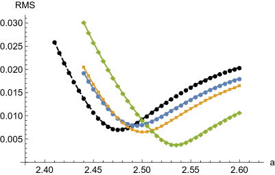
Figure 1: (Colour on-line) Root-mean-square of linear fit to points $(1/L,\chi/L^{a})$ plotted versus $a$ for PBC (black), $A_{1}$ (blue), $A_{2}$ (orange) and $A_{4}$ (green). Minimum at respectively $2.475$, $2.49$, $2.50$, $2.535$.

Continuing with the $B_{r}$-case we show RMS versus $a$ in Fig. 2. The mean of the minima centre around $2.275(10)$, where we have used $L\geq 23$ for the fitted line. It would perhaps be natural to expect the linear fit to favour the mid-point $2.25$ between $2$ and $2.5$ but this is not supported by the present data. It should be remarked that, the mean value of the minima is remarkably stable between different point sets but the individual minima vary between $2.255$ and $2.29$. Hence we suggest that the correct $a$-value is a little larger than $2.25$.

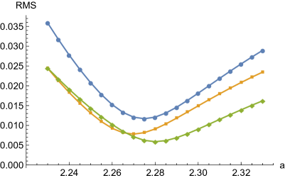
Figure 2: (Colour on-line) Root-mean-square of linear fit to points $(1/L,\chi/L^{a})$ plotted versus $a$ for $B_{1}$ (blue), $B_{2}$ (orange) and $B_{4}$ (green). Minimum at $2.275$, $2.27$, $2.28$, respectively.

Finally, the case of $C_{r}$ (thus including FBC) is shown in Fig. 3. The RMS-plots clearly prefer an exponent close to $2$. With the present linear fit, using $L\geq 19$, we find an average minimum $2.00(1)$. Trying different point sets gives almost the same average but individual minima varies between $1.97$ and $2.015$.

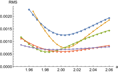
Figure 3: (Colour on-line) Root-mean-square of linear fit to points $(1/L,\chi/L^{a})$ plotted versus $a$ for $C_{1}$ (blue, values divided by 3), $C_{2}$ (orange), $C_{3}$ (green), $C_{4}$ (red) and $C_{5}$ (purple). Minimum at respectively $2.005$, $2.005$, $1.985$, $2.000$, $1.995$.

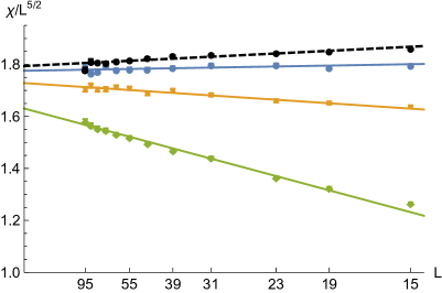
Figure 4: (Colour on-line) Normalised susceptibility $\chi/L^{5/2}$ versus $1/L$ for $L=15$, $19$, $23$, $31$, $39$, $47$, $55$, $63$, $71$, $79$, $87$ and $95$. Cases are PBC (black), $A_{1}$ (blue), $A_{2}$ (orange) and $A_{4}$ (green). Fitted lines are, respectively, $y=1.794+1.11x$, $y=1.775+0.40x$, $y=1.729-1.50x$, $y=1.630-6.0x$ where $x=1/L$.

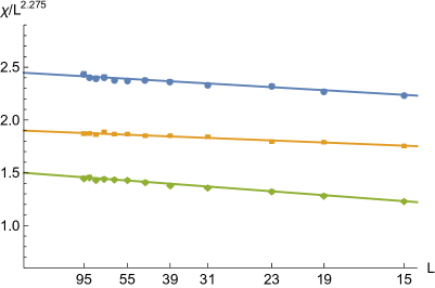
Figure 5: (Colour on-line) Normalised susceptibility $\chi/L^{2.275}$ versus $1/L$ for $L=15$, $19$, $23$, $31$, $39$, $47$, $55$, $63$, $71$, $79$, $87$ and $95$. Cases are $B_{1}$ (blue), $B_{2}$ (orange) and $B_{4}$ (green). Fitted lines are, respectively, $y=2.45-3.1x$, $y=1.90-2.2x$, $1.50-4.0x$ where $x=1/L$.

In Figs. 4, 5 and 6 we show the normalised susceptibility $\chi/L^{a}$ versus $1/L$ together with the fitted lines $y=c_{0}+c_{1}x$ from which we read the asymptotic value $c_{0}$. This very simple rule appears quite sufficient and we see no prescense of any higher-order correction terms. In fact, plotting $c_{1}=L(\chi/L^{a}-c_{0})$ versus $1/L$ is effectively constant (modulo noise, increasing with $L$). We show here only the case of $B_{r}$ in Fig. 7 but the other cases results in quite similar plots.

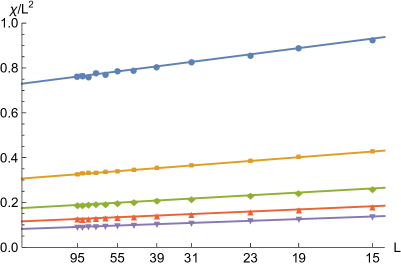
Figure 6: (Colour on-line) Normalised susceptibility $\chi/L^{2}$ versus $1/L$ for $L=15$, $19$, $23$, $31$, $39$, $47$, $55$, $63$, $71$, $79$, $87$ and $95$. Cases are (downwards) $C_{1}$ (blue), $C_{2}$ (orange), $C_{3}$ (green), $C_{4}$ (red) and $C_{5}$ (purple). Fitted lines are, respectively, $y=0.730+3.0x$, $y=0.307+1.8x$, $0.175+1.3x$, $y=0.116+1.0x$, $y=0.082+0.83x$ where $x=1/L$.

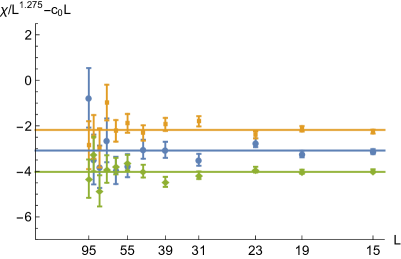
Figure 7: (Colour on-line) $L(\chi/L^{2.275}-c_{0})$ versus $1/L$ for $L=15$, $19$, $23$, $31$, $39$, $47$, $55$, $63$, $71$, $79$, $87$ and $95$. Cases are $B_{1}$ (blue), $B_{2}$ (orange) and $B_{4}$ (green). Values of $c_{0}$ are, respectively, $2.45$, $1.90$, $1.50$. Constant lines are, respectively, $y=-3.1$, $y=-2.2$, $y=-4.0$. See Fig. 5

IV Magnetisation distribution

We will here make an attempt to describe the distribution of the magnetisation. Beginning with the kurtosis $\operatorname{\mathcal{K}}$ for PBC we expect it to take the asymptotic value $\Gamma(1/4)^{4}/(8\pi^{2})\approx 2.1884$ Brezin and Zinn-Justin (1985) and for FBC we expect it to be $3$, as is characteristic for a normal distribution.

In general the mean-field density function Binder et al. (1985); Brezin and Zinn-Justin (1985)

$$f(x)=c_{0}\exp(-c_{2}x^{2}-c_{4}x^{4})$$ (7)

fits these distributions very well, except for very small systems where a correction factor is needed. Note that the case $c_{2}=0$ gives the kurtosis $2.1884$ mentioned above for all $c_{4}>0$. The distribution then is unimodal when $c_{2}>0$ giving $\operatorname{\mathcal{K}}>2.1884$ and a bimodal distribution when $c_{2}<0$ corresponding to $\operatorname{\mathcal{K}}<2.1884$. The function $f(x)$ can now be determined from the variance and the kurtosis. We will here only show the standardised form (variance $1$).

The kurtosis plotted in Fig. 8 demonstrate an interesting feature with regard to the distribution shape. Since the cases PBC and $A_{1}$ all have $\operatorname{\mathcal{K}}<2.1884$ they are thus bimodal but converge to a “flat” distribution ($c_{2}=0$). However, in the case of $A_{2}$ the kurtosis is almost constant $\approx 2.2$ for all $L$, just barely unimodal. For $A_{4}$ we are safely into unimodal territory though.

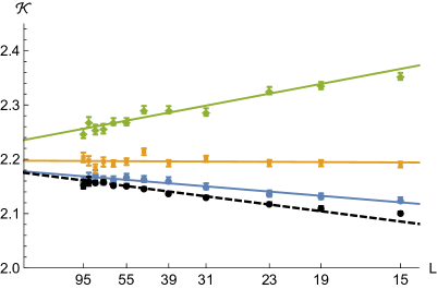
Figure 8: (Colour on-line) Magnetisation kurtosis $\operatorname{\mathcal{K}}(\beta_{c})$ versus $L$ for $L=15$, $19$, $23$, $31$, $39$, $47$, $55$, $63$, $71$, $79$, $87$ and $95$. Cases are, PBC (black, dashed curve), $A_{1}$ (blue), $A_{2}$ (orange) and $A_{4}$ (green). Lines fitted to $L\geq 19$ give asymptotic values, respectively, $2.18(1)$, $2.18(1)$, $2.20(1)$, $2.24(1)$.

In Fig. 9 we show an example of a standardised distribution in the $A_{2}$-case for $L=63$. Based on the kurtosis we find the density function $f(x)$ numerically. Here $\operatorname{\mathcal{K}}=2.1922$ which gives $f(x)=0.3213\exp(-0.004541x^{2}-0.1130x^{4})$, where $x=M/\sigma$. A Pearson goodness-of-fit test is now used to see if we should reject the hypothesis that $f(x)$ fits the magnetisation distribution. In fact we find $\chi^{2}/\mathrm{dof}\approx 0.96$ for $\mathrm{dof}=200$ and a $p$-value of $0.61$ so we choose not to reject this.

This was repeated for the other cases (three $A_{r}$) and sizes (twelve $L$) as well, using $\lceil 2n_{s}^{2/5}\rceil$ equiprobable bins (Mathematica’s default) for $n_{s}$ samples. Median $p$-value over these $36$ instances is $0.50$ with interquartile range $0.47$ and all were larger than $0.05$. The hypothesis that the distribution is described by Eq. (7) is thus not rejected for $A_{r}$ and $L\geq 15$.

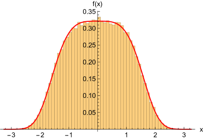
Figure 9: (Colour on-line) Standardised magnetisation distribution density for $A_{2}$-case, $L=63$. Kurtosis $\operatorname{\mathcal{K}}=2.192(6)$ gives $f(x)=0.3213\exp(-0.00445x^{2}-0.113x^{4})$ (red curve) where $x=M/\sigma$. A Pearson goodness-of-fit test is passed with $p$-value $0.61$.

Moving on to the case $B_{r}$ we show the magnetisation kurtosis in Fig. 10 and it does not appear to converge to $3$ for any of these cases. The distributions still fit Eq. (7) though. The Pearson test gave the median $p$-value $0.71$ and an interquartile range of $0.48$ and only one of the 36 instances ($r=1$, $L=55$) gave $p<0.05$. Since $5$% of the instances will fail even if the hypothesis is true we find this quite normal. We thus do not reject that Eq. (7) fits these distributions for $B_{r}$ and $L\geq 15$. In Fig. 11 we show an example of this distribution and $f(x)$ for $B_{1}$ and $L=63$.

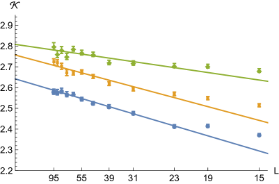
Figure 10: (Colour on-line) Magnetisation kurtosis $\operatorname{\mathcal{K}}(\beta_{c})$ versus $L$ for $L=15$, $19$, $23$, $31$, $39$, $47$, $55$, $63$, $71$, $79$, $87$ and $95$. Cases are $B_{1}$ (blue), $B_{2}$ (orange) and $B_{4}$ (green). Lines fitted to $L\geq 23$ give asymptotic values, respectively, $2.64(1)$, $2.76(1)$, $2.81(1)$.

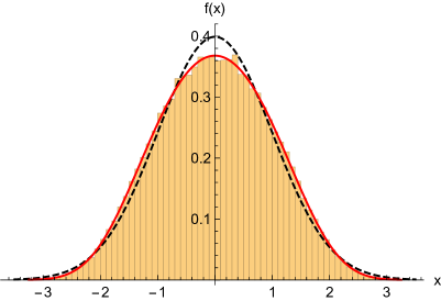
Figure 11: (Colour on-line) Standardised magnetisation distribution density for $L=63$ with edges $B_{1}$. Kurtosis $\operatorname{\mathcal{K}}=2.568(9)$ gives $f(x)=0.3680\exp(-0.327x^{2}-0.0338x^{4})$ (red curve) where $x=M/\sigma$. Dashed black curve is density of a normal distribution. A Pearson goodness-of-fit test is passed with $p$-value $0.80$.

For the $C_{r}$-case the kurtosis is close to $3$ (modulo noise) in almost all instances. Only for $r=1$ do we see a weak trend with values clearly distinct from $3$ for the smallest $L$ (no figure). We tested the hypothesis that the distribution of the magnetisation samples are Gaussian for all $r$ and $L\geq 23$. Indeed, of these $50$ instances only $4$ ($8$%) fail ($p$-value less than $0.05$) which is to be expected. The median $p$-value over the instances was $0.46$ with interquartile range $0.45$. Thus we do not reject the hypothesis.

V Scaling of energy quantities

Let us first discuss the finite-size scaling of the internal energy $\operatorname{\mathcal{U}}$. Across the different cases the data seem to agree on the common limit energy $\operatorname{\mathcal{U}}(\beta_{c})=0.6756(1)$. For PBC a very simple scaling rule $\operatorname{\mathcal{U}}_{L}=c_{0}+c_{1}/L^{5/2}$ is sufficient. For $A_{r}$ we suggest $\operatorname{\mathcal{U}}_{L}=c_{0}+c_{1}/L^{5/2}+c_{2}/L^{5}$, though the choice of the second exponent is uncertain.

At the other end of the spectrum, for FBC and $C_{r}$, the rule $\operatorname{\mathcal{U}}_{L}=c_{0}+c_{1}/L+c_{2}/L^{3/2}$ gives stable scaling, also used in Ref. Lundow and Markström (2014). For $B_{r}$ the rule $\operatorname{\mathcal{U}}_{L}=c_{0}+c_{1}/L+c_{2}/L^{5/2}$ gives stable behaviour when deleting points. These scaling rules gives the limit value $c_{0}=0.6756(1)$ above but we seem unable to provide any more digits. Needless to say, we have no theory-based support for these scaling rules. In Fig. 12 we plot the energy versus $1/L$ for all cases and sizes together with fitted curves as just described.

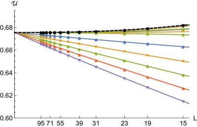
Figure 12: (Colour on-line) Energy $\operatorname{\mathcal{U}}$ versus $L$ for $L=15$, $19$, $23$, $31$, $39$, $47$, $55$, $63$, $71$, $79$, $87$ and $95$. Boundary conditions are (downwards) PBC (black, dashed curve), $A_{r}$ ($r=1,2,4$), $B_{r}$ ($r=1,2,4$) and $C_{r}$ ($r=1,\ldots,5$) The fitted curves (see text) have the common limit $0.6756(1)$, Error bars are shown but smaller than the points.

Since the specific heat is bounded for 5D systems Sokal (1979) one might expect its finite-size scaling to be similar to that of the energy. Unfortunately the scaling rules above do not seem to apply to the specific heat. In Fig. 13 we therefore plot the specific heat together with fitted 2nd degree polynomials which at least provides rough estimates of the limit values.

For PBC we estimate the limit $\operatorname{\mathcal{C}}(\beta_{c})\approx 54.0(5)$ (marginally less than in Ref. Lundow and Markström (2015)). In the $A_{r}$-case we obtain the limits $53.0(5)$, $52.0(5)$, $50.0(5)$ for $r=1,2,4$, respectively. The $B_{r}$-case gives $22.5(5)$, $19.0(5)$, $16.5(5)$ for $r=1,2,4$, respectively. Finally, the $C_{r}$-case resulted in the (probably) common estimate $12.5(5)$, though the noise is larger than the differences between the estimated limits.

In Ref. Lundow and Markström (2014) only one correction term was used with exponent $1/3$ for FBC, so that $\operatorname{\mathcal{C}}_{L}=c_{0}+c_{1}/L^{1/3}$. All $C_{r}$-instances are indeed well-fitted by this elegant rule, but this would lead to a limit of $14.7$ for $C_{5}$ (FBC), larger than the resulting limit $12.6$ for $C_{1}$. Hence, we hesitate to use this simple rule since all data suggest that the specific heat should decrease when deleting boundary edges, just like the energy does in Fig. 12.

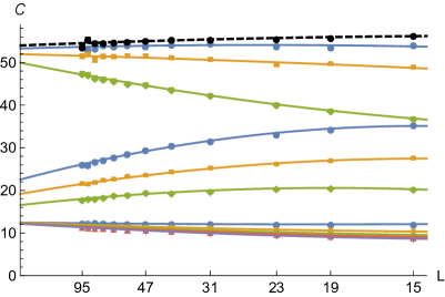
Figure 13: (Colour on-line) Specific heat $\operatorname{\mathcal{C}}$ versus $L$ for $L=15$, $19$, $23$, $31$, $39$, $47$, $55$, $63$, $71$, $79$, $87$ and $95$. Boundary conditions are (downwards at $y$-axis) PBC (black, dashed curve), $A_{r}$ ($r=1,2,4$), $B_{r}$ ($r=1,2,4$) and $C_{r}$ ($r=1,\ldots,5$). Limit values range from $54$ for PBC to $12.5$ for FBC (see text). Error bars are shown but smaller than the points.

In Fig. 14 we see the effect that the boundary has on the skewness of the energy distribution. At the top of the figure we see that PBC and $A_{r}$ are almost indistinguishable and they all agree on a common limit value of $1.023(5)$ based on fitted lines. For PBC and $A_{1}$ the skewness is effectively constant (modulo noise) over $L$. There is only a very small size-dependence for $A_{2}$ and $A_{4}$.

For $B_{r}$ the skewness has clearly separated itself from PBC. Also, the size-dependence becomes clearly nonlinear. Fitting 2nd degree polynomials to the points we estimate the limits $0.72(1)$, $0.50(1)$ and $0.31(1)$ for $r=1,2,4$ respectively (error bars from deleting one point in the fit). In the $C_{r}$-case the skewness is practically zero for all $L$ for $r=2,3,4,5$ but there is a distinct (almost) linear size-dependence for $r=1$, becoming effectively zero for $L\geq 47$.

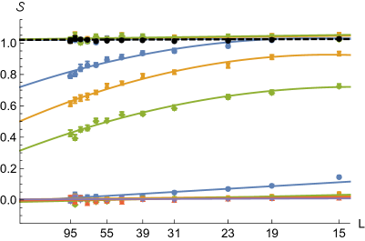
Figure 14: (Colour on-line) Energy skewness $\operatorname{\mathcal{S}}$ versus $L$ for $L=15$, $19$, $23$, $31$, $39$, $47$, $55$, $63$, $71$, $79$, $87$ and $95$. Boundary conditions are: at the top, PBC (black, dashed curve) and $A_{r}$ ($r=1,2,4$, indistinguishable); middle three, $B_{r}$ ($r=1,2,4$ downwards); at the bottom, $C_{r}$ ($r=1,\ldots,5$, with $r=1$ deviating). Limit values range from $1.02$ for PBC and $A_{r}$ to $0$ for FBC (see text for details). Error bars are shown but often smaller than the points.

The kurtosis $\operatorname{\mathcal{K}}$ of the energy distribution is shown in Fig. 15. At this point the pattern is clear. PBC and $A_{r}$ behave similarly (dashed curves in the figure), though $A_{4}$ stands out, with limit values $4.48(1)$ (PBC), $4.39(4)$ ($r=1$), $4.56(3)$ ($r=2$) and $4.46(3)$ ($r=4$), with error bars estimated by removing one point at a time from a fitted 2nd degree polynomial. Since the error bars are larger for $A_{r}$ they could in fact have a common limit value $4.48$. In Fig. 16 we show the energy distribution for PBC ($L=79$), which is quite similar to that of $A_{r}$.

For $B_{r}$ (solid curves in figure) we estimate the limits $4.43(3)$ ($r=1$), $3.93(3)$ ($r=2$) and $3.55(3)$ ($r=4$) from fitted 2nd degree polynomials. Possibly the $r=1$-case has the same limit value as PBC. The $C_{r}$-case all favour the estimate $3.00(1)$ by way of fitted lines, but there is a small size dependence for $r=1$.

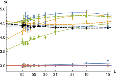
Figure 15: (Colour on-line) Energy kurtosis $\operatorname{\mathcal{K}}$ versus $L$ for $L=15$, $19$, $23$, $31$, $39$, $47$, $55$, $63$, $71$, $79$, $87$ and $95$. Boundary conditions are: at the top, PBC (black, dashed curve) and $A_{r}$ ($r=1,2,4$, (blue, orange, green; dashed curves); $B_{r}$ ($r=1,2,4$ blue, orange, green; solid curves); at the bottom, $C_{r}$ ($r=1,\ldots,5$, with $r=1$ deviating). See text for limit values. Error bars are shown but sometimes smaller than the points.

We performed a Pearson goodness-of-fit test to compare the energy distributions of $C_{r}$ to a Gaussian distribution. For $r=2,\ldots,5$, this test is passed for all $L\geq 31$, giving a median $p$-value of $0.47$ and interquartile range $0.34$ over the 36 instances. However, for $r=1$ we need $L\geq 63$ to pass the test on the 5%-level..

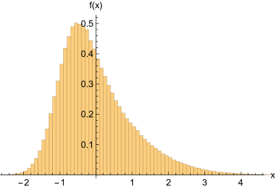
Figure 16: (Colour on-line) Standardised energy distribution density for PBC, $L=79$, $n_{s}=500000$. This instance has energy $\operatorname{\mathcal{U}}=0.6756$, specific heat $\operatorname{\mathcal{C}}=54.7$, skewness $\operatorname{\mathcal{S}}=1.03$ and kurtosis $\operatorname{\mathcal{K}}=4.44$. Note that $x=(E-\left\langle E\right\rangle)/\sqrt{\mathrm{var}\!\left(E\right)}$.

VI Conclusion

We have investigated several scenarios of deleting boundary edges from a PBC-system, where an FBC-system corresponds to deleting $5L^{4}$ edges. For example, what happens to the finite-size scaling of the susceptibility when we delete all boundary edges in only one direction, i.e., $L^{4}$ edges? Remarkably, we find that this is enough to switch the scaling behaviour to that associated with FBC. The distribution of magnetisations, essentially distributed as $c_{0}\exp(-c_{4}x^{4})$ for PBC, has also switched to Gaussian for $L\geq 23$, to the extent that it passes a Pearson goodness-of-fit test.

Deleting just $L^{2}$ boundary edges does not change the scaling behaviour significantly from that of PBC though it does increase the kurtosis slightly, making the distribution of magnetisations unimodal. However, deleting $L^{3}$ boundary edges changes the susceptibility scaling to something strictly inbetween PBC and FBC, we estimate that $\chi\propto L^{2.275}$.

We also note that all magnetisation distributions are well-fitted by the simple formula in Eq. (7), passing a Pearson test to the expected degree.

The energy-related quantities also change when deleting boundary edges, though correction-to-scaling terms give less than clear scaling rules. We suggest that deleting $rL^{4}$ edges ($C_{r}$-case) may all give the same specific heat limit value of $12.5(5)$, for $r=1,\ldots,5$. Deleting just $rL^{2}$ edges, and for that matter, $rL^{3}$ edges, gives us specific heat values inbetween PBC and FBC.

The energy skewness is essentially the same for PBC and when deleting $rL^{2}$ edges, $\operatorname{\mathcal{S}}\to 1.02$. Deleting $rL^{4}$ edges gives $\operatorname{\mathcal{S}}\to 0$. Deleting $rL^{3}$ edges gives limit values inbetween these two.

The energy kurtosis for PBC and when deleting $rL^{2}$ edges may have the same limit value, say $4.5$, but there is too much noise to say with any certainty. Deleting $rL^{4}$ puts the kurtosis close to 3 and, as we may expect, a Pearson test suggests the energy distribution is essentially Gaussian in this case, if $L$ is large enough. However, deleting $rL^{3}$ edges puts the kurtosis somewhere inbetween, possibly $r=1$ may give the same limit as PBC.

One may well wonder how this generalises to higher dimensions. For example, starting with a 6D system with periodic boundary conditions we expect the finite-size scaling $\chi\propto L^{3}$. If we delete the $L^{5}$ boundary edges along one direction, is this enough to change the scaling to $\chi\propto L^{2}$? What happens when we delete $L^{4}$, $L^{3}$, $L^{2}$ edges?