Trade-offs in learning controllers from noisy data

Abstract

In data-driven control, a central question is how to handle noisy data. In this work, we consider the problem of designing a stabilizing controller for an unknown linear system using only a finite set of noisy data collected from the system. For this problem, many recent works have considered a disturbance model based on energy-type bounds. Here, we consider an alternative more natural model where the disturbance obeys instantaneous bounds. In this case, the existing approaches, which would convert instantaneous bounds into energy-type bounds, can be overly conservative. In contrast, without any conversion step, simple arguments based on the S-procedure lead to a very effective controller design through a convex program. Specifically, the feasible set of the latter design problem is always larger, and the set of system matrices consistent with data is always smaller and decreases significantly with the number of data points. These findings and some computational aspects are examined in a number of numerical examples.

1 Introduction

Problem formulation and related work

In the last few years, there has been a renewed growing interest towards data-driven control. Data-driven control provides an alternative tool for control design whenever modeling based on first principles is difficult or impossible [22, 21] and it has been employed for robust and optimal control [2, 13], predictive control [10, 1], and control of nonlinear [23] and time-varying systems [20].

In this paper, we start from a basic control problem, that is, designing a controller by a finite set of data with $T$ samples collected from a system. Specifically, for state $x\in\mathbb{R}^{n}$, input $u\in\mathbb{R}^{m}$ and disturbance $d\in\mathbb{R}^{n}$, we apply an input sequence $\{u(0),\dots,u(T-1)\}$ to a linear time-invariant discrete-time system and measure the state sequence $\{x(0),\dots,x(T)\}$ generated as response as

$$x(i+1)=A_{\star}x(i)+B_{\star}u(i)+d(i),\quad i=0,\dots,T-1.$$ (1)

The matrices $A_{\star}$ and $B_{\star}$ are unknown and we do not have access to disturbance $d$, so data are noisy. The objective is to use the input and (noisy) state sequence to design a feedback control law $u=Kx$ to solve a stabilization problem, that is, ensuring that $A_{\star}+B_{\star}K$ has eigenvalues with magnitude strictly less than 1 (Schur stability).

Albeit basic, this problem poses many challenges. In fact, since $d$ in (1) affects the state sequence, it is impossible to uniquely reconstruct the system matrices $A_{\star}$ and $B_{\star}$ from the input and state sequences; instead, we have a set of possible matrices that could have generated the state sequence. Accordingly, the problem corresponds to a robust stabilization problem in the face of the uncertainty introduced by $d$, entailing a set of matrices to stabilize rather than a singleton. In the literature, several works have considered problems of this type, in the very same setting as here [13, 3, 4, 25], or in other settings like linear-quadratic-regulator design [15, 27, 14], robust set invariance [6], switched and nonlinear systems [11, 12, 17, 7].

In all aforementioned works, the starting point is to define a model for the disturbance. Typical choices on opposite sides of the spectrum are disturbances with known probability distributions or statistics (e.g., $d$ is assumed a white Gaussian noise [15, 27, 14]) or the so-called unknown-but-bounded models, as we consider in this paper. In unknown-but-bounded models, $d$ may be a deterministic function of time or a stochastic process and the only characteristic assumed to be known is that $d$ is contained in a given region [13, 25, 3, 4, 14, 6, 11, 17, 7]. In this setting, a natural way to describe the uncertainty is to consider instantaneous constraints for $d$ as

$$\mathcal{D}_{\textup{i}}:=\{d\in\mathbb{R}^{n}\colon|d|^{2}\leq\epsilon\}$$ (2)

where $\epsilon\geq 0$ represents our prior knowledge on $d$. This model naturally arises in many practical cases (e.g., with process load disturbances), and it has a long history in set-constrained control and set-membership identification [16, 5, 18]. As an alternative to instantaneous constraints, one can consider energy constraints on $d$ as

$$\mathcal{D}_{\textup{e}}:=\big{\{}d^{0},d^{1},\dots,d^{T-1}\in\mathbb{R}^{n}\colon\!\sum_{i=0}^{T-1}d^{i}(d^{i})^{\top}\preceq\epsilon_{\textup{e}}I\big{\}}$$ (3)

where $d^{0},d^{1},\dots,d^{T-1}$ correspond to any disturbance sequence and $\epsilon_{\textup{e}}\geq 0$ represents our prior knowledge on the disturbance sequence. This model (or similar ones involving quadratic bounds on the possible disturbance sequences) has been considered in many recent works on data-driven control [13, 25, 3, 4]. The reason for considering $\mathcal{D}_{\textup{e}}$ is essentially technical. By using $\mathcal{D}_{\textup{e}}$, the uncertainty set of system matrices consistent with data is given by a single quadratic matrix inequality and this enables deriving simple stability conditions [13, Thm. 5], or even necessary and sufficient conditions under a mild regularity property on data as in [25, Thm. 14]. From a practical viewpoint, however, this disturbance model is artificial. In fact, $\mathcal{D}_{\textup{e}}$ is typically built starting from $\mathcal{D}_{\textup{i}}$, i.e., by setting $\epsilon_{\textup{e}}=\epsilon T$; see [3, §IV], [25, Ex. 3] and [4, §VI]. As a consequence, the bound $\epsilon_{\textup{e}}=\epsilon T$ in (3) increases with $T$ and this may lead to a set of data-consistent system matrices that grows with $T$ (see Example 1) so that using larger data sets may even be detrimental, which is undesirable and counterintuitive. Among the aforementioned recent works, few considered instantaneous bounds. They were used in [11, 12] for data-driven control of switched and polynomial systems, where the problem was reduced to a nonconvex quadratic program and then relaxed to a polynomial optimization problem. Working directly with $\mathcal{D}_{\textup{i}}$ was also pursued in [4, §V] as a secondary development, by using sum-of-squares relaxations.

Paper contribution

In this paper, we investigate pros and cons of using directly an instantaneous bound instead of translating it into an energy bound. We show that working with $\mathcal{D}_{\textup{i}}$ is indeed advantageous since (i) the uncertainty set resulting from $\mathcal{D}_{\textup{i}}$ is never larger than the one resulting from $\mathcal{D}_{\textup{e}}$ with $\epsilon_{\textup{e}}=\epsilon T$; (ii) there exist simple design methods that work directly with $\mathcal{D}_{\textup{i}}$ and always return a stabilizing solution whenever the methods based on $\mathcal{D}_{\textup{e}}$ do. We also show that the extra numerical cost due to working with $\mathcal{D}_{\textup{i}}$ is quite modest up to large sets of data. Compared to [4], our method rests on simpler arguments and uses design tools purely based on linear matrix inequalities (instead of polynomial constraint qualification conditions that may be hard to assess). As an auxiliary contribution, we introduce a notion of size for matrix ellipsoids to numerically measure the uncertainty induced by $d$. This measure confirms that the uncertainty resulting from $\mathcal{D}_{\textup{i}}$ is typically order of magnitudes smaller than that resulting from $\mathcal{D}_{\textup{e}}$.

Structure

Section 2 obtains a size notion for matrix ellipsoids. In Section 3, we present the controller design problems for the energy-bound and instantaneous-bound approach, and relate them in terms of feasibility. In Section 4, we further compare the two approaches by examining the corresponding sets of dynamical matrices consistent with data. The numerical investigation in Section 5 completes the comparison, and leads to the conclusions of Section 6.

2 Preliminaries

In this section, we set up the notation and introduce a notion of size for matrix ellipsoids, which will be used in the numerical simulations of Section 5.

2.1 Notation

For a matrix $A$, $|A|$ denotes its induced 2-norm. Given two matrices $A$ and $B$, $A\otimes B$ denotes their Kronecker product. For a matrix $A=\begin{bmatrix}a_{1}&\cdots&a_{n}\end{bmatrix}\in\mathbb{R}^{m\times n}$ partitioned according to its columns, $\operatorname{vec}(A):=[a_{1}^{\top}\,\,\,\cdots\,\,\,a_{n}^{\top}]^{\top}$ denotes its vectorization. A property of vectorization is that, for matrices $A,X,B$ and $C$ of compatible dimensions, the matrix equation $AXB=C$ is equivalent to $(B^{\top}\otimes A)\operatorname{vec}(X)=\operatorname{vec}(C)$ [19, Lemma 4.3.1]. For fixed natural numbers $m$ and $n$, the inverse of the vectorization operator takes as input a vector $a=[a_{1}^{\top}\,\,\,\cdots\,\,\,a_{n}^{\top}]^{\top}\in\mathbb{R}^{mn}$ partitioned in components $a_{1},\dots,a_{n}\in\mathbb{R}^{m}$ and returns

$$\operatorname{vec}^{-1}_{m,n}(a):=\begin{bmatrix}a_{1}&\dots&a_{n}\end{bmatrix}\in\mathbb{R}^{m\times n}.$$ (4)

For matrices $A$, $B$ and $C$ of compatible dimensions, we abbreviate $ABC(AB)^{\top}$ to $AB\cdoT C[\star]^{\top}$, where the dot in the second expression clarifies unambiguously that $AB$ are the terms to be transposed.

2.2 A size notion for matrix ellipsoids

For symmetric matrices $\mathsf{P}\in\mathbb{R}^{p\times p}$, $\mathsf{Q}\in\mathbb{R}^{q\times q}$, $\mathsf{A}\in\mathbb{R}^{p\times p}$, $\mathsf{C}\in\mathbb{R}^{q\times q}$ and matrices $\mathsf{Z}_{\textup{c}}\in\mathbb{R}^{p\times q}$, $\mathsf{B}\in\mathbb{R}^{p\times q}$, we term matrix ellipsoid a set in one of the next two forms:

$$\mathcal{E}_{\textup{mat}} :=\{\mathsf{Z}\in\mathbb{R}^{p\times q}\colon(\mathsf{Z}-\mathsf{Z}_{\textup{c}})^{\top}\mathsf{P}^{-2}(\mathsf{Z}-\mathsf{Z}_{\textup{c}})\preceq\mathsf{Q}\},$$ (5a)

$$\mathcal{E}_{\textup{mat}}^{\prime} :=\{\mathsf{Z}\in\mathbb{R}^{p\times q}\colon\mathsf{Z}^{\top}\mathsf{A}\mathsf{Z}+\mathsf{Z}^{\top}\mathsf{B}+\mathsf{B}^{\top}\mathsf{Z}+\mathsf{C}\preceq 0\}$$ (5b)

where

$$\mathsf{P}\succ 0,\mathsf{Q}\succ 0\text{ ~{}and~{} }\mathsf{A}\succ 0,\mathsf{B}^{\top}\mathsf{A}^{-1}\mathsf{B}-\mathsf{C}\succ 0.$$ (6)

The constraints $\mathsf{Q}\succ 0$ and $\mathsf{B}^{\top}\mathsf{A}^{-1}\mathsf{B}-\mathsf{C}\succ 0$ ensure that $\mathcal{E}_{\textup{mat}}$ and $\mathcal{E}_{\textup{mat}}^{\prime}$ are not empty or do not reduce to a singleton; the constraints $\mathsf{P}\succ 0$ and $\mathsf{A}\succ 0$ ensure that the matrix ellipsoid is a bounded set. We stress that many sets considered in the sequel (e.g., $\mathcal{C}$ in Section 3.1 and $\overline{\mathcal{I}}$ in Section 5.1) have to be expressed in terms of these matrix ellipsoids, and that (5a) and (5b) are natural extensions of the classical ellipsoids in the Euclidean space, cf. [8, Eqs. (3.8)-(3.9)].

Standard computations reformulate $\mathcal{E}_{\textup{mat}}^{\prime}$ as

$$\mathcal{E}_{\textup{mat}}^{\prime} =\{\mathsf{Z}\in\mathbb{R}^{p\times q}\colon(\mathsf{Z}+\mathsf{A}^{-1}\mathsf{B})^{\top}\mathsf{A}(\mathsf{Z}+\mathsf{A}^{-1}\mathsf{B})$$

$$\hskip 99.58464pt-(\mathsf{B}^{\top}\mathsf{A}^{-1}\mathsf{B}-\mathsf{C})\preceq 0\}.$$ (7)

Hence, $\mathcal{E}_{\textup{mat}}$ and $\mathcal{E}_{\textup{mat}}^{\prime}$ are the same set for

$$\mathsf{Z}_{\textup{c}}=-\mathsf{A}^{-1}\mathsf{B},\,\mathsf{P}^{-2}=\mathsf{A},\,\mathsf{Q}=\mathsf{B}^{\top}\mathsf{A}^{-1}\mathsf{B}-\mathsf{C}.$$ (8)

Let us focus on $\mathcal{E}_{\textup{mat}}$ to define a size. Since $\mathsf{Q}\succ 0$, $\mathcal{E}_{\textup{mat}}$ is equivalently written as

$$\mathcal{E}_{\textup{mat}} \!=\!\{\mathsf{Z}\!\in\mathbb{R}^{p\times q}\colon\mathsf{Q}^{-1/2}(\mathsf{Z}-\mathsf{Z}_{\textup{c}})^{\top}\mathsf{P}^{-2}(\mathsf{Z}-\mathsf{Z}_{\textup{c}})\mathsf{Q}^{-1/2}\!\preceq I\}$$

$$\!=\!\{\mathsf{Z}_{\textup{c}}+\mathsf{P}\mathsf{Y}\mathsf{Q}^{1/2}\colon\mathsf{Y}\in\mathbb{R}^{p\times q},\mathsf{Y}^{\top}\mathsf{Y}\preceq I\}$$

where $\mathsf{Y}^{\top}\mathsf{Y}\preceq I$ is equivalent to $|\mathsf{Y}|\leq 1$. Then, we specify the measure space in question and the adopted measure. Given natural numbers $p$ and $q$, $\operatorname{vec}\colon\mathbb{R}^{p\times q}\to\mathbb{R}^{pq}$ is a bijection between $\mathbb{R}^{p\times q}$ and $\mathbb{R}^{pq}$ with inverse $\operatorname{vec}^{-1}_{p,q}\colon\mathbb{R}^{pq}\to\mathbb{R}^{p\times q}$. With $\mathcal{P}(\mathcal{T})$ denoting the power set of a set $\mathcal{T}$, we define the bijection $\mathcal{V}\colon\mathcal{P}(\mathbb{R}^{p\times q})\to\mathcal{P}(\mathbb{R}^{pq})$ as

$$\mathcal{V}(\mathcal{S}):=\{\operatorname{vec}(s)\colon s\in\mathcal{S}\}$$

for $\mathcal{S}\subseteq\mathbb{R}^{p\times q}$. Then, its inverse $\mathcal{V}^{-1}$ satisfies $\mathcal{V}^{-1}(\mathcal{S}_{\textup{v}})=\{\operatorname{vec}^{-1}_{p,q}(s_{\textup{v}})\colon s_{\textup{v}}\in\mathcal{S}_{\textup{v}}\}$ for $\mathcal{S}_{\textup{v}}\subseteq\mathbb{R}^{pq}$. By using standard notions in measure theory [24, §1.2, §1.4], we consider in $\mathbb{R}^{pq}$ the standard collection $\mathcal{B}_{\textup{v}}$ of Lebesgue measurable sets as $\sigma$-algebra and for $\beta_{\textup{v}}\in\mathcal{B}_{\textup{v}}$, $m(\beta_{\textup{v}})$ is the Lebesgue measure of the set $\beta_{\textup{v}}$. With $\mathcal{B}_{\textup{v}}$ and $m$, we can define a $\sigma$-algebra $\mathcal{B}$ in $\mathbb{R}^{p\times q}$ as $\mathcal{B}:=\{\mathcal{V}^{-1}(\beta_{\textup{v}})\colon\beta_{\textup{v}}\in\mathcal{B}_{\textup{v}}\}$ and then, for each $\beta\in\mathcal{B}$, a measure $\mu$ as $\mu(\beta):=m(\mathcal{V}(\beta))$. This makes $(\mathbb{R}^{p\times q},\mathcal{B},\mu)$ a measure space [24, Def. 1.4.27]. For $\mathsf{z}_{\textup{c}}:=\operatorname{vec}\mathsf{Z}_{\textup{c}}$, let

$$\begin{split}\mathcal{E}_{\textup{vec}}&:=\mathcal{V}(\mathcal{E}_{\textup{mat}})\\ &=\{\mathsf{z}_{\textup{c}}+(\mathsf{Q}^{1/2}\otimes\mathsf{P})\mathsf{y}\colon\mathsf{y}\in\mathbb{R}^{pq},|\operatorname{vec}^{-1}_{p,q}(\mathsf{y})|\leq 1\},\end{split}$$

which is closed, and thus Lebesgue measurable [24, Lemma 1.2.13]. Accordingly, $\mathcal{E}_{\textup{mat}}\!$ belongs to $\mathcal{B}$ and its measure is

$$\mu(\mathcal{E}_{\textup{mat}})=m(\mathcal{E}_{\textup{vec}})=:\operatorname{vol}(\mathcal{E}_{\textup{vec}})$$ (9)

where it is standard to identify the volume of $\mathcal{E}_{\textup{vec}}$ with its Lebesgue measure (see, e.g., [9, p. 105]). The next lemma determines $\operatorname{vol}(\mathcal{E}_{\textup{vec}})$.

Lemma 1.

Let $p$ and $q$ be given natural numbers, and let $\mathsf{Q}\in\mathbb{R}^{q\times q}$ and $\mathsf{P}\in\mathbb{R}^{p\times p}$ be symmetric positive definite matrices. Then,

$$\operatorname{vol}(\mathcal{E}_{\textup{vec}})=\beta(\det\mathsf{Q})^{\frac{p}{2}}(\det\mathsf{P})^{q}$$

where $\beta$ is a constant that depends only on $p$ and $q$.

Proof.

Let

$$\overline{\mathcal{E}}_{\textup{vec}}:=\{(\mathsf{Q}^{1/2}\otimes\mathsf{P})\mathsf{y}\colon\mathsf{y}\in\mathbb{R}^{pq},|\operatorname{vec}^{-1}_{p,q}(\mathsf{y})|\leq 1\}.$$

By translation invariance [24, Exercise 1.2.20], $m(\overline{\mathcal{E}}_{\textup{vec}})=m(\mathcal{E}_{\textup{vec}})$. The set $\{\mathsf{y}\in\mathbb{R}^{pq}\colon|\operatorname{vec}^{-1}_{p,q}(\mathsf{y})|\leq 1\}$ is closed, thus Lebesgue measurable. By [24, Exercise 1.2.21],

$$m(\overline{\mathcal{E}}_{\textup{vec}})=\det(\mathsf{Q}^{1/2}\otimes\mathsf{P})m\big{(}\{\mathsf{y}\in\mathbb{R}^{pq}\colon|\operatorname{vec}^{-1}_{p,q}(\mathsf{y})|\leq 1\}\big{)}.$$

The last term in this expression depends only on $p$ and $q$ and $\det(\mathsf{Q}^{1/2}\otimes\mathsf{P})=(\det\mathsf{Q})^{\frac{p}{2}}(\det\mathsf{P})^{q}$ by Kronecker-product properties [19, §4.2, Problem 1]. ∎

In view of (9) and Lemma 1, the set $\mathcal{E}_{\textup{mat}}$ has measure $\mu(\mathcal{E}_{\textup{mat}})=\beta(\det\mathsf{Q})^{\frac{p}{2}}(\det\mathsf{P})^{q}$. The constant $\beta$ is analogous to the proportionality constant in [8, p. 42], which is the volume of the $2$-norm unit ball. The precise expression of $\beta$ is irrelevant for our developments because we will compare only matrix ellipsoids with same $p$ and $q$. Hence, we disregard $\beta$ and define the size of $\mathcal{E}_{\textup{mat}}$ simply as

$$(\det\mathsf{Q})^{\frac{p}{2}}(\det\mathsf{P})^{q}.$$

Since the sets $\mathcal{E}_{\textup{mat}}$ and $\mathcal{E}_{\textup{mat}}^{\prime}$ are the same when the correspondences in (8) hold, their size is in that case

$$(\det\mathsf{Q})^{\frac{p}{2}}(\det\mathsf{P})^{q}\!=\!(\det(\mathsf{B}^{\top}\mathsf{A}^{-1}\mathsf{B}-\mathsf{C}))^{\frac{p}{2}}(\det(\mathsf{A}^{-1}))^{\frac{q}{2}}.$$ (10)

Both terms in this expression reduce to classical volume formulae for $\mathsf{Z}\in\mathbb{R}^{p\times 1}$ [8, p. 42].

3 Data-consistent dynamics and controller design problems

In this section we return to our original problem of designing a stabilizing controller for (1) from a finite data set. We first determine the set of system matrices consistent with the data points when the disturbance model is given by $\mathcal{D}_{\textup{i}}$ or $\mathcal{D}_{\textup{e}}$, and then formulate the corresponding control design problems. From (2), (3) and $\epsilon_{\textup{e}}=\epsilon T$ as discussed in Section 1, we have

$$\mathcal{D}_{\textup{i}}= \{d\in\mathbb{R}^{n}\colon|d|^{2}\leq\epsilon\}=\{d\in\mathbb{R}^{n}\colon dd^{\top}\preceq\epsilon I\}$$ (11a)

$$\mathcal{D}_{\textup{e}}= \Big{\{}d^{0},\dots,d^{T-1}\in\mathbb{R}^{n}\colon T\epsilon I-\sum_{i=0}^{T-1}d^{i}(d^{i})^{\top}$$

$$\hskip 2.27621pt=\left[\begin{array}[]{c|ccc}\!\!I\!&d^{0}\!\!\!&\dots\!\!\!&d^{T-1}\!\!\end{array}\right]\!\cdoT\!\begin{bmatrix}T\epsilon I&0\\ 0&-I\end{bmatrix}[\star]^{\top}\!\succeq 0\Big{\}}.$$ (11c)

For notational convenience, all data points are grouped as

$$X_{1} :=\begin{bmatrix}x(1)&x(2)&\cdots&x(T)\end{bmatrix}$$

$$X_{0} :=\begin{bmatrix}x(0)&x(1)&\cdots&x(T-1)\end{bmatrix}$$

$$U_{0} :=\begin{bmatrix}u(0)&u(1)&\cdots&u(T-1)\end{bmatrix}$$

and the set of their relevant indices $i$ is $\mathbb{I}:=\{0,\dots,T-1\}$.

3.1 Dynamics consistent with the data

We call consistent with data all the matrices $(A,B)$ that, for the selected input sequence, could have generated the measured state sequence while keeping $d$ in the bound $\mathcal{D}_{\textup{e}}$ in (11c) or $\mathcal{D}_{\textup{i}}$ in (11a), and we characterize the corresponding two sets in this section.

Based on the bound in (11c), the matrices $(A,B)$ consistent with the data points are in

$$\begin{split}&\mathcal{C}:=\Big{\{}(A,B)\colon D\in\mathbb{R}^{n\times T},X_{1}=AX_{0}+BU_{0}+D,\\ &\hskip 71.13188pt\begin{bmatrix}I&D\end{bmatrix}\begin{bmatrix}T\epsilon I&0\\ 0&-I\end{bmatrix}\begin{bmatrix}I\\ D^{\top}\end{bmatrix}\succeq 0\Big{\}},\end{split}$$ (12)

i.e., all those matrices for which some disturbance sequence satisfying the bound in (11c) could have generated the measured data. By eliminating $D$ in (12), $\mathcal{C}$ rewrites as

$$\mathcal{C}=\Big{\{}(A,B)\colon\begin{bmatrix}I&A&B\end{bmatrix}\begin{bmatrix}I&X_{1}\\ 0&-X_{0}\\ 0&-U_{0}\end{bmatrix}\cdoT\begin{bmatrix}T\epsilon I&0\\ 0&-I\end{bmatrix}[\star]^{\top}\succeq 0\Big{\}}.$$ (13)

Analogously, based on the bound in (11a), the matrices $(A,B)$ consistent with a data point $i\in\mathbb{I}$ are in

$$\begin{split}&\mathcal{C}_{i}:=\Big{\{}(A,B)\colon d\in\mathbb{R}^{n},\\ &\hskip 34.1433ptx(i+1)=Ax(i)+Bu(i)+d,\,dd^{\top}\preceq\epsilon I\Big{\}},\end{split}$$ (14)

i.e., all those matrices for which some disturbance $d$ satisfying the bound in (11a) could have generated the measured data point $i$. By eliminating $d$ in (14), $\mathcal{C}_{i}$ rewrites as

$$\mathcal{C}_{i}=\Big{\{}(A,B)\colon\begin{bmatrix}I&A&B\end{bmatrix}\begin{bmatrix}I&x(i+1)\\ 0&-x(i)\\ 0&-u(i)\end{bmatrix}\cdoT\begin{bmatrix}\epsilon I&0\\ 0&-I\end{bmatrix}[\star]^{\top}\succeq 0\Big{\}}.$$ (15)

The expression of $\mathcal{C}_{i}$ in (15) mirrors that of $\mathcal{C}$ in (13), which was the reason to write $dd^{\top}\preceq\epsilon I$ in (14) instead of the equivalent but more immediate $|d|^{2}\leq{\epsilon}$. The set of matrices $(A,B)$ consistent with all data points is then

$$\mathcal{I}:=\bigcap_{i=0}^{T-1}\mathcal{C}_{i}.$$ (16)

When neglecting the constraint $\mathsf{A}\succ 0$ in (6), both the sets $\mathcal{C}$ and $\mathcal{C}_{i}$ can be expressed in the form (5b) of matrix ellipsoids. Indeed, the inequalities constituting the sets $\mathcal{C}$ in (13) and $\mathcal{C}_{i}$ in (15) can be equivalently written as

$$\begin{bmatrix}A&B\end{bmatrix}\mathsf{A}_{j}\begin{bmatrix}A^{\top}\\ B^{\top}\end{bmatrix}+\begin{bmatrix}A&B\end{bmatrix}\mathsf{B}_{j}+\mathsf{B}_{j}^{\top}\begin{bmatrix}A^{\top}\\ B^{\top}\end{bmatrix}+\mathsf{C}_{j}\preceq 0$$ (17a)

where the matrices $$\mathsf{A}_{j},\mathsf{B}_{j} \mathsf{C}_{j} j=\mathbb{I} \mathcal{C} j=i \mathcal{C}_{i} \mathsf{Z}^{\top}=\begin{bmatrix}A&B\end{bmatrix} \mathcal{C} \mathsf{A}_{\mathbb{I}}\succ 0 \left[\begin{smallmatrix}X_{0}\\ U_{0}\end{smallmatrix}\right] \mathsf{A}_{i}\succ 0 \mathcal{C}_{i} \mathcal{I} \mathcal{C}_{i} \mathcal{I}\subseteq\mathcal{C} \mathcal{I} \mathcal{C}$$, with for and for are defined in (17b), displayed below over two columns. This corresponds to (5b) with . We note two facts. The set is not necessarily bounded. It is bounded if or, equivalently, the matrix has full row rank. This condition expresses the property that data are sufficiently rich in content, and is related to the notion of persistency of excitation [26]. On the other hand, condition for is never satisfied. However, this is irrelevant since the set of interest when dealing with instantaneous bounds is , formed by the intersection of all as in (16). We will prove below in Proposition 3 that , which guarantees that is bounded whenever is.

$$\mathsf{C}_{\mathbb{I}}:=-T\epsilon I+X_{1}X_{1}^{\top},~{}\mathsf{B}_{\mathbb{I}}:=-\begin{bmatrix}X_{0}\\ U_{0}\end{bmatrix}X_{1}^{\top},~{}\mathsf{A}_{\mathbb{I}}:=\begin{bmatrix}X_{0}\\ U_{0}\end{bmatrix}\begin{bmatrix}X_{0}\\ U_{0}\end{bmatrix}^{\top},~{}\mathsf{C}_{i}:=-\epsilon I+x(i+1)x(i+1)^{\top},~{}\mathsf{B}_{i}:=-\begin{bmatrix}x(i)\\ u(i)\end{bmatrix}x(i+1)^{\top},~{}\mathsf{A}_{i}:=\begin{bmatrix}x(i)\\ u(i)\end{bmatrix}\begin{bmatrix}x(i)\\ u(i)\end{bmatrix}^{\top}$$ (17b)

3.2 Controller design methods

We now formulate the control design problems related to the two sets $\mathcal{C}$ and $\mathcal{I}$, i.e., to the energy bound $\mathcal{D}_{\textup{e}}$ and to the instantaneous bound $\mathcal{D}_{\textup{i}}$.

The energy-bound approach solves:

find $$P\succ 0,K$$

s.t. $$(A+BK)P(A+BK)^{\top}-P\prec 0$$ (18)

$$\hskip 19.91692pt\text{ for all }(A,B)\text{ such that }(A,B)\in\mathcal{C}$$

where the condition in the second line expresses discrete-time asymptotic stability. The instantaneous-bound approach solves:

find $$P\succ 0,K$$

s.t. $$(A+BK)P(A+BK)^{\top}-P\prec 0$$ (19)

$$\hskip 19.91692pt\text{ for all }(A,B)\text{ such that }(A,B)\in\mathcal{I}.$$

Both the feasibility problems (18) and (19) correspond to robust stabilization in the face of the uncertainty introduced by $d$, which induces a set of matrices to stabilize rather than a singleton. We stress that we consider here a stabilization problem as a prototypical control problem, but our main conclusions would apply unchanged to other control problems like $\mathcal{L}_{2}$ gain minimization or $\mathcal{H}_{\infty}$ control.

By the lossless matrix S-procedure [25, Thm. 12] and Schur complement, the result [25, Thm. 13] shows that, under a mild regularity condition on data, feasibility of (18) is equivalent to feasibility of

find $$P,Y,\beta,\alpha$$

s.t. $$\left[\begin{array}[]{cccc}P-\beta I&0&0&0\\ 0&-P&-Y^{\top}&0\\ 0&-Y&0&Y\\ 0&0&Y^{\top}&P\end{array}\right]$$ (24)

$$\hskip 2.84526pt-\alpha\left[\begin{array}[]{cc}I&X_{1}\\ 0&-X_{0}\\ 0&-U_{0}\\ 0&0\end{array}\right]\left[\begin{array}[]{cc}T\epsilon I&0\\ 0&-I\end{array}\right]\left[\begin{array}[]{cc}I&X_{1}\\ 0&-X_{0}\\ 0&-U_{0}\\ 0&0\end{array}\right]^{\top}\succeq 0$$ (35)

$$\alpha\geq 0,\beta>0,P\succ 0$$

where now the decision variables appear linearly. If (24) has a solution, $K=YP^{-1}$ is a stabilizing controller for (1).

On the other hand, a tractable equivalent reformulation of (19) based on matrix ellipsoids cannot be obtained. Indeed, even in the simplest case where $n=m=1$, the set $\mathcal{I}$ is an intersection of ellipsoids and finding the ellipsoid with minimum volume containing $\mathcal{I}$ is NP-complete [8, p. 44]. Hence, finding such an ellipsoid and applying then the necessary and sufficient conditions in [25, Thm. 12] is impractical. To pursue an alternative approach, we need the next lemma, which is an immediate extension to matrices of the classic lossy S-procedure [8, §2.6.3].

Lemma 2.

Let $T_{0}$, …, $T_{\ell}\in\mathbb{R}^{(q+p)\times(q+p)}$ be symmetric matrices. If there exist nonnegative scalars $\tau_{1},\dots,\tau_{\ell}$ such that $T_{0}-\sum_{i=1}^{\ell}\tau_{i}T_{i}\succeq 0$, then $\left[\begin{smallmatrix}I\\ Z\end{smallmatrix}\right]^{\top}T_{0}\left[\begin{smallmatrix}I\\ Z\end{smallmatrix}\right]\succeq 0$ for all $Z\in\mathbb{R}^{p\times q}$ such that $\left[\begin{smallmatrix}I\\ Z\end{smallmatrix}\right]^{\top}T_{i}\left[\begin{smallmatrix}I\\ Z\end{smallmatrix}\right]\succeq 0$ for each $i=1,\dots,\ell$.

Proof.

For an arbitrary $Z$ satisfying $\left[\begin{smallmatrix}I\\ Z\end{smallmatrix}\right]^{\top}T_{i}\left[\begin{smallmatrix}I\\ Z\end{smallmatrix}\right]\succeq 0$ for each $i=1,\dots,\ell$, use the condition $T_{0}-\sum_{i=1}^{\ell}\tau_{i}T_{i}\succeq 0$ to obtain $\left[\begin{smallmatrix}I\\ Z\end{smallmatrix}\right]^{\top}T_{0}\left[\begin{smallmatrix}I\\ Z\end{smallmatrix}\right]\succeq 0$. ∎

We use the lossy matrix S-procedure in Lemma 2 and obtain a sufficient condition to guarantee feasibility of (19) in the next proposition.

Proposition 1.

Feasibility of

find $$P,Y,\beta,\tau_{0},\dots,\tau_{T-1}$$

s.t. $$\left[\begin{array}[]{@{}cccc@{}}P-\beta I&0&0&0\\ 0&-P&-Y^{\top}&0\\ 0&-Y&0&Y\\ 0&0&Y^{\top}&P\end{array}\right]$$ (40)

$$\hskip 2.84526pt-\sum_{i=0}^{T-1}\tau_{i}\left[\begin{array}[]{@{}cc@{}}I&x(i+1)\\ 0&-x(i)\\ 0&-u(i)\\ 0&0\end{array}\right]\left[\begin{array}[]{@{}cc@{}}\epsilon I&0\\ 0&-I\end{array}\right]\left[\begin{array}[]{@{}cc@{}}I&x(i+1)\\ 0&-x(i)\\ 0&-u(i)\\ 0&0\end{array}\right]^{\top}\succeq 0$$ (51)

$$\beta>0,\tau_{0}\geq 0,\dots,\tau_{T-1}\geq 0,P\succ 0,$$

implies feasibility of (19).

Proof.

Condition $(A+BK)P(A+BK)^{\top}-P\prec 0$ in (19) is equivalent to the existence of a positive scalar $\beta$ such that $(A+BK)P(A+BK)^{\top}-P\preceq-\beta I$, i.e.,

$$\begin{bmatrix}I&A&B\end{bmatrix}\cdoT\begin{bmatrix}P-\beta I&0&0\\ 0&-P&-PK^{\top}\\ 0&-KP&-KPK^{\top}\end{bmatrix}[\star]^{\top}\succeq 0.$$

By Schur complement and change of variable $Y=KP$, (3.2) is equivalent to

find $$P,K,\beta,\tau_{0},\dots,\tau_{T-1}$$

s.t. $$\left[\begin{array}[]{@{}cccc@{}}P-\beta I&0&0\\ 0&-P&-PK^{\top}\\ 0&-KP&-KPK^{\top}\\ \end{array}\right]$$

$$\hskip 2.84526pt-\sum_{i=0}^{T-1}\tau_{i}\left[\begin{array}[]{@{}cc@{}}I&x(i+1)\\ 0&-x(i)\\ 0&-u(i)\\ \end{array}\right]\left[\begin{array}[]{@{}cc@{}}\epsilon I&0\\ 0&-I\end{array}\right]\left[\begin{array}[]{@{}cc@{}}I&x(i+1)\\ 0&-x(i)\\ 0&-u(i)\\ \end{array}\right]^{\top}\succeq 0$$

$$\beta>0,\tau_{0}\geq 0,\dots,\tau_{T-1}\geq 0,P\succ 0.$$

By Lemma 2, feasibility of this problem implies feasibility of (19), which proves the statement. ∎

As in (24), the decision variables appear linearly in (3.2) and solving (3.2) yields the controller gain $K=YP^{-1}$. With respect to (24), solving (3.2) involves $T$ scalar variables $\tau_{i}$ instead of a single one $\alpha$. Having as many decision variables as the number of data points may be computationally demanding with (very) large data sets. We will further elaborate on this point later in Section 5.3.

The feasibility properties of (24) and (3.2) are related. In particular, the next proposition shows that solving (3.2) is as easy or easier than solving (24).

Proposition 2.

If (24) is feasible, (3.2) is feasible.

Proof.

Consider a feasible solution to (24) for some variables $P$, $Y$, $\beta$, $\alpha$, and note that

$$\begin{split}\begin{bmatrix}I&X_{1}\\ 0&-X_{0}\\ 0&-U_{0}\\ 0&0\end{bmatrix}\cdoT\begin{bmatrix}T\epsilon I&0\\ 0&-I\end{bmatrix}[\star]^{\top}=\sum_{i=0}^{T-1}\begin{bmatrix}I&x(i+1)\\ 0&-x(i)\\ 0&-u(i)\\ 0&0\end{bmatrix}\cdoT\begin{bmatrix}\epsilon I&0\\ 0&-I\end{bmatrix}[\star]^{\top}\end{split}.$$

Thus, the same variables $P$, $Y$, $\beta$ with $\tau_{0}=\dots=\tau_{T-1}=\alpha\geq 0$ provide a feasible solution to (3.2). ∎

In the next section, we aim at quantifying the gap in terms of feasibility. To this end, we shift the focus from the design problems (18) and (19) to the corresponding sets $\mathcal{C}$ and $\mathcal{I}$ because (18) and (19) impose the very same stability condition on $\mathcal{C}$ and $\mathcal{I}$, respectively. Hence, the smaller $\mathcal{C}$ or $\mathcal{I}$ is, the larger the feasible set [9, §4.1.1] of the design problems (18) or (19) is. Next section will actually show that $\mathcal{I}\subseteq\mathcal{C}$.

4 Comparison between energy and instantaneous bounds: Theoretical evidence

In this section, we firstly show a monotonicity property of the set $\mathcal{I}$ with respect to the number $T$ of data points, and, secondly, a relation between the sets $\mathcal{C}$ and $\mathcal{I}$.

Firstly, to illustrate monotonicity properties, we would like to highlight the dependence of $\mathcal{C}$ and $\mathcal{I}$ on the number $T$ of data points. With some notation abuse, we then write equivalently $\mathcal{C}$ or $\mathcal{C}(T)$, and $\mathcal{I}$ or $\mathcal{I}(T)$. It is immediate that

$$\mathcal{I}(T+1)\subseteq\mathcal{I}(T)$$ (52)

because $\mathcal{I}(T+1)$ contains precisely the same constraints as $\mathcal{I}(T)$ plus an additional one. This is a desirable property because we expect more data to reduce the uncertainty by providing additional information, or, in the worst case, to keep the uncertainty at the same level. On the other hand, we build the next example to show that $\mathcal{C}(T+1)\subseteq\mathcal{C}(T)$ does not hold in general.

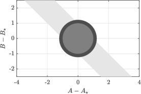
Figure 1: The sets $\mathcal{C}(1)$, $\mathcal{C}(2)$, $\mathcal{C}(3)$ defined in Example 1 correspond respectively to light, medium, dark gray.

Example 1.

Consider in (1) $A_{\star}=1/2$ and $B_{\star}=1/2$ as the unknown dynamical matrices. Assume that $x(0)=1$, $u(0)=1$, $u(1)=-1$, $u(2)=0$, $d(0)=d(1)=d(2)=0$, and that the disturbance bound is $\epsilon=1$, These sequences give $x(1)=1$, $x(2)=x(3)=0$. Define for brevity $\tilde{A}:=A-A_{\star}$ and $\tilde{B}:=B-B_{\star}$. With some computations, (13) yields for $T=1,2,3$

$$\mathcal{C}(1) =\{(A,B)\colon 1-\tilde{A}^{2}-\tilde{B}^{2}-2\tilde{A}\tilde{B}\geq 0\}$$

$$\mathcal{C}(2) =\{(A,B)\colon 2-2\tilde{B}^{2}-2\tilde{A}^{2}\geq 0\}$$

$$\mathcal{C}(3) =\{(A,B)\colon 3-2\tilde{B}^{2}-2\tilde{A}^{2}\geq 0\},$$

which are depicted in Fig. 1. The ellipsoid corresponding to $\mathcal{C}(T)$ does not always shrink with larger $T$, but more data (such as when $T$ goes from $2$ to $3$) can actually induce larger bounds in an undesirable way.

Secondly, the next proposition provides a relation between $\mathcal{C}$ and $\mathcal{I}$, which corroborates Proposition 2.

Proposition 3.

The relation $\mathcal{I}\subseteq\mathcal{C}$ holds.

Proof.

We assume that $(A,B)$ belongs to $\mathcal{I}=\bigcap_{i=0}^{T-1}\mathcal{C}_{i}$, and show that, then, $(A,B)$ belongs to $\mathcal{C}$. Let us then manipulate the left-hand side of the inequality in (13) as

$$\begin{bmatrix}I&A&B\end{bmatrix}\begin{bmatrix}I&X_{1}\\ 0&-X_{0}\\ 0&-U_{0}\end{bmatrix}\cdoT\begin{bmatrix}T\epsilon I&0\\ 0&-I\end{bmatrix}[\star]^{\top}$$

$$=\begin{bmatrix}I&A&B\end{bmatrix}\begin{bmatrix}I&x(1)&\dots&x(T)\\ 0&-x(0)&\dots&-x(T-1)\\ 0&-u(0)&\dots&-u(T-1)\end{bmatrix}\cdoT\begin{bmatrix}T\epsilon I&0\\ 0&-I\end{bmatrix}[\star]^{\top}$$

$$=\sum_{i=0}^{T-1}\Big{(}\epsilon I-(x(i+1)-Ax(i)-Bu(i))\cdoT[\star]^{\top}\Big{)}.$$

Each term of the sum is positive semidefinite since $(A,B)$ is assumed to belong to $\bigcap_{i=0}^{T-1}\mathcal{C}_{i}$, hence the whole sum is positive semidefinite. This proves that $(A,B)\in\mathcal{C}$. ∎

Proposition 3 establishes that the set $\mathcal{I}$ is contained in, or at most equal to, the set $\mathcal{C}$. We are going to show now through numerical experiments that the former set actually has size significantly smaller than the latter.

5 Comparison between energy and instantaneous bounds: Numerical evidence

In this section, we complement the theoretical results in Propositions 2 and 3 with numerical evidence showing the actual relation between $\mathcal{I}$ and $\mathcal{C}$, their dependence on $T$, and the impact of these two aspects on feasibility of the control design problems. For this comparison, we preliminarily obtain in Section 5.1 an over-approximation of $\mathcal{I}$. We note that this over-approximation, although providing insights on this comparison, does not play any role in controller design.

5.1 Overapproximation $\overline{\mathcal{I}}$ of the set $\mathcal{I}$

Whereas the size of $\mathcal{C}$ can be obtained as in Section 2.2, a measure of $\mathcal{I}:=\bigcap_{i=0}^{T-1}\mathcal{C}_{i}$ is difficult to obtain exactly. In fact, $\mathcal{I}$ is an intersection of matrix ellipsoids, and for $n=m=1$, even finding the ellipsoid of minimum volume containing $\mathcal{I}$ is NP-complete [8, p. 44]. We thus set up a convex optimization problem to obtain a computable over-approximation $\overline{\mathcal{I}}$ of $\mathcal{I}$. Considering $\overline{\mathcal{I}}$ for the comparison with $\mathcal{C}$ is relevant because, albeit being an over-approximation, its size is still (significantly) smaller than the size of $\mathcal{C}$ in all the subsequent numerical examples.

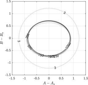
Figure 2: The ellipsoids inside the dashed lines correspond to $\mathcal{C}$ for $T=3,250,500,750,1000$, as the labels indicate. The larger $T$, the darker the dashed line.

We assume that the set $\mathcal{I}$ is bounded, cf. Section 3.1. Using the approach in [8, §3.7.2] for classical ellipsoids, we find a matrix ellipsoid $\overline{\mathcal{I}}$ that includes all $\mathcal{C}_{i}$’s through the lossy S-procedure in Lemma 2, and we minimize the size of $\overline{\mathcal{I}}$, defined in Section 2.2. We take $\overline{\mathcal{I}}$ as

$$\overline{\mathcal{I}} :=\{(A,B)\colon\big{[}\begin{array}[]{@{}c|cc@{}}I&A&B\end{array}\big{]}\begin{bmatrix}\overline{\mathsf{C}}~{}&\overline{\mathsf{B}}^{\top}\\ \overline{\mathsf{B}}~{}&\overline{\mathsf{A}}\end{bmatrix}\left[\begin{array}[]{@{}c@{}}I\\ \hline\cr\phantom{\rule{0.1pt}{10.0pt}}A^{\top}\\ B^{\top}\end{array}\right]\preceq 0\}$$

$$=\{(A,B)\colon\overline{\mathsf{C}}+\overline{\mathsf{B}}^{\top}\begin{bmatrix}A^{\top}\\ B^{\top}\end{bmatrix}+\begin{bmatrix}A&B\end{bmatrix}\overline{\mathsf{B}}+\begin{bmatrix}A&B\end{bmatrix}\overline{\mathsf{A}}\begin{bmatrix}A^{\top}\\ B^{\top}\end{bmatrix}\preceq 0\}$$

where we set $\overline{\mathsf{C}}=\overline{\mathsf{B}}^{\top}\overline{\mathsf{A}}^{-1}\overline{\mathsf{B}}-I$ (otherwise the representation of $\overline{\mathcal{I}}$ is homogeneous) and require $\overline{\mathsf{A}}\succ 0$ so that (6) holds. We impose $\mathcal{I}=\bigcap_{i=0}^{T-1}\mathcal{C}_{i}\subseteq\overline{\mathcal{I}}$ via the lossy matrix S-procedure in Lemma 2, and obtain

$$\begin{bmatrix}\overline{\mathsf{B}}^{\top}\overline{\mathsf{A}}^{-1}\overline{\mathsf{B}}\!-\!I&\,\overline{\mathsf{B}}^{\top}\\ \overline{\mathsf{B}}&\,\overline{\mathsf{A}}\end{bmatrix}-\sum_{i=0}^{T-1}\tau_{i}\begin{bmatrix}\mathsf{C}_{i}&\mathsf{B}_{i}^{\top}\\ \mathsf{B}_{i}&\mathsf{A}_{i}\end{bmatrix}\preceq 0,\tau_{i}\geq 0\text{ for }i\in\mathbb{I}$$

with $\mathsf{C}_{i}$, $\mathsf{B}_{i}$, $\mathsf{A}_{i}$ defined in (17b). Since the first inequality is nonlinear in the decision variables $\overline{\mathsf{B}}$ and $\overline{\mathsf{A}}$, we rewrite it by Schur complement as

$$\begin{bmatrix}\vspace*{1pt}-I-\sum_{i=0}^{T-1}\tau_{i}\mathsf{C}_{i}&\overline{\mathsf{B}}^{\top}-\sum_{i=0}^{T-1}\tau_{i}\mathsf{B}_{i}^{\top}&\overline{\mathsf{B}}^{\top}\\ \vspace*{1pt}\overline{\mathsf{B}}-\sum_{i=0}^{T-1}\tau_{i}\mathsf{B}_{i}&\overline{\mathsf{A}}-\sum_{i=0}^{T-1}\tau_{i}\mathsf{A}_{i}&0\\ \overline{\mathsf{B}}&0&-\overline{\mathsf{A}}\end{bmatrix}\preceq 0.$$ (53)

By (10), the size of $\overline{\mathcal{I}}$ is given by $(\det\overline{\mathsf{A}})^{-\frac{n}{2}}$ thanks to the adopted normalization. These constraints and objective function result in the optimization problem

minimize $$-\log\det\overline{\mathsf{A}}$$ (54)

subject to $$\eqref{bigContainCond},\,\overline{\mathsf{A}}\succ 0,\,\tau_{i}\geq 0\text{ for }i\in\mathbb{I}.$$

When $n=m=1$, this optimization problem boils down to that in [8, Eq. (3.15)], but (54) also captures the case of generic dimensions $n$ and $m$, as we need in the following.

5.2 A visualizable example

In this section we examine more thoroughly the system of Example 1 and show how the sizes of $\mathcal{C}$ and $\mathcal{I}$ depend on $T$ and how they compare with each other.

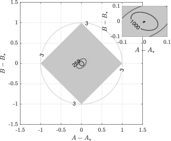
Figure 3: The shaded areas correspond to $\mathcal{I}$ and are barely visible for $T\geq 250$, as can be appreciated in the inset. The ellipsoids inside the dashed lines correspond to $\overline{\mathcal{I}}$ (we omit some labels for readability). Increasingly darker color for the areas and lines correspond to $T=3,250,500,750,1000$.

We prolong the data sequences of Example 1 by using as input and disturbance the realizations of random variables uniformly distributed in $[-2,2]$ and $[-{\epsilon},{\epsilon}]=[-1,1]$, respectively. The resulting set $\mathcal{C}$, depicted for $T=3$ in Fig. 1, is now depicted for some $T$ up to $1000$ in Fig. 2. Fig. 2 shows that the energy-based ellipsoids $\mathcal{C}$ shrink very slowly as $T$ increases, and stay approximately constant from $T=250$ on. The resulting set $\mathcal{I}$ is depicted for the same values of $T$ in Fig. 3 together with its over-approximation $\overline{\mathcal{I}}$, determined as in Section 5.1. Fig. 3 shows that the ellipsoids $\overline{\mathcal{I}}$ shrink very quickly with $T$ and, albeit only over-approximations of $\mathcal{I}$, they are significantly smaller than the ellipsoids $\mathcal{C}$. The actual sets $\mathcal{I}$, which are depicted by shaded areas, shrink even faster to the point that they are barely visible already for $T=250$.

For a clearer visualization, Fig. 4 depicts the ratio between the sizes of $\mathcal{C}$ and $\overline{\mathcal{I}}$. $\overline{\mathcal{I}}$ is smaller than $\mathcal{C}$ by more than 30 times already with approximately $200$ data points.

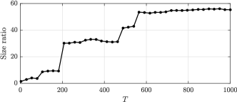
Figure 4: Ratio between the sizes of $\mathcal{C}$ and $\overline{\mathcal{I}}$, Section 5.2.

5.3 Example with third order dynamics

In this section, we delve into the considerations of Section 5.2 through a more complex example with matrices

$$A_{\star}=\begin{bmatrix}0.1274&0.1431&0.1974\\ 0.3619&0.6292&0.4153\\ 0.6972&0.1574&0.4111\end{bmatrix}\!,\,B_{\star}=\begin{bmatrix}0.6901&0.9047\\ 0.4809&0.6030\\ 0.8913&0.1478\end{bmatrix}.$$

A data set is obtained by applying the realization of a Gaussian random variable (zero mean and unit standard deviation) as input, and as disturbance the realization of a random variable distributed uniformly in $\{d\colon|d|^{2}\leq{\epsilon}\}$ with different values for ${\epsilon}$.

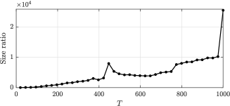
Figure 5: Ratio between the sizes of $\mathcal{C}$ and $\overline{\mathcal{I}}$, Section 5.3.

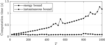
Figure 6: Computation times for controller design in (24) and (3.2).

As in the previous example, we compare the sizes of $\mathcal{C}$ and of $\overline{\mathcal{I}}$ assuming $\epsilon=0.1$. Their ratio is plotted in Fig. 5 for increasingly larger portions of data from $T=20$ up to $T=1000$. The size of $\overline{\mathcal{I}}$ is smaller than $\mathcal{C}$ by approximately two orders of magnitude already with $100$ data points. We commented after Proposition 1 that the energy-based approach (24) requires $T-1$ scalar decision variables less than the formulation in (3.2). We show numerically that the impact of these extra variables is modest even with a large number of data. The computations times to solve (24) or (3.2) are depicted in Fig. 6. The controller design in (24) has the appealing feature that the associated computation time barely changes with the number of data points whereas (3.2) exhibits a dependence on $T$ that results in a computation time that grows linearly with $T$.

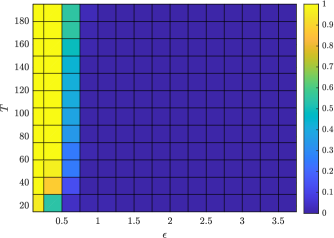
Figure 7: Energy-bound approach (24): the color represents for each disturbance bound $\epsilon$ and data length $T$ the ratio of feasible controller design problems in a batch of 100.

Finally, we examine the joint effect of the disturbance bound $\epsilon$ and of the length $T$ on both the approaches. For each value of $\epsilon$ and $T$, we solve a batch of 100 feasibility problems (24) or (3.2), count the number $n_{\textup{feas}}$ of feasible ones in that batch and display the ratio $n_{\textup{feas}}/100\in[0,1]$ in Figs. 7–8 through a color code. Yellow areas are the good ones in terms of feasibility. Fig. 7 depicts this ratio for the energy-bound approach and shows that above a threshold $\epsilon$ of approximately $0.7$, the problem (24) has no solutions regardless of the number of data. This behaviour seems consistent with what we observed in Fig. 2 about the fact that the set of consistent matrices is not reduced by larger amounts of data. Fig. 8 depicts the ratio $n_{\textup{feas}}/100$ for the instantaneous-bound approach, and shows its appealing feature of being able to withstand increasingly larger disturbance magnitudes as long as an increasingly number of data points is collected to reduce uncertainty. Comparing Figs. 5–6 with Figs. 7–8, we can conclude that the price paid in terms of computation time is negligible compared with the gain in terms of robustness.

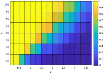
Figure 8: Instantaneous-bound approach (3.2), see caption of Fig. 7.

6 Conclusions

In this paper, we compared two different disturbance models for data-driven control design: a model $\mathcal{D}_{\textup{e}}$ considering energy bounds on the entire disturbance sequence and a model $\mathcal{D}_{\textup{i}}$ considering instantaneous bounds on the disturbance. The model $\mathcal{D}_{\textup{e}}$ leads to elegant necessary and sufficient condition for stability, and results in a design program whose number of variables depends only on the dimensions of the system to be controlled and not on the number of data points. On the other hand, the model $\mathcal{D}_{\textup{i}}$ reflects a much more natural way of describing disturbances.

We analyzed pros and cons of working directly with $\mathcal{D}_{\textup{i}}$, instead of converting it into $\mathcal{D}_{\textup{e}}$. The analysis shows that, computational considerations aside, it is in fact always preferable to work with $\mathcal{D}_{\textup{i}}$. First, $\mathcal{D}_{\textup{i}}$ results in a design program that is always feasible whenever the one associated with $\mathcal{D}_{\textup{e}}$ is feasible. Second, numerical evidence shows that the feasibility gap can be extremely large. This latter aspect has been analyzed by introducing a notion of size for the uncertainty set induced by the disturbance. Simulations show that while the uncertainty set associated with $\mathcal{D}_{\textup{e}}$ does not necessarily shrink, the one associated with $\mathcal{D}_{\textup{i}}$ often shrinks very quickly, and is many order of magnitudes smaller. As for computational considerations, working with $\mathcal{D}_{\textup{i}}$ is less advantageous because it results in a design program whose number of variables depends on the number of data points. With the exception of extremely large data sets, however, the price paid in terms of computation time appears negligible compared with the advantages offered in terms of robustness.

References

- [1] A. Allibhoy and J. Cortés. Data-based receding horizon control of linear network systems. IEEE Control Systems Letters, 5(4):1207–1212, 2021.
- [2] G. Baggio, V. Katewa, and F. Pasqualetti. Data-driven minimum-energy controls for linear systems. IEEE Control Systems Letters, 3(3):589–594, 2019.
- [3] J. Berberich, A. Romer, C. W. Scherer, and F. Allgöwer. Robust data-driven state-feedback design. In Proc. Amer. Control Conf., 2020.
- [4] J. Berberich, C. W. Scherer, and F. Allgöwer. Combining prior knowledge and data for robust controller design. arXiv preprint arXiv:2009.05253, 2020.
- [5] D. Bertsekas and J. Rhodes. Recursive state estimation for a set-membership description of uncertainty. IEEE Trans. Autom. Control, 16(2):117–128, 1971.
- [6] A. Bisoffi, C. De Persis, and P. Tesi. Controller design for robust invariance from noisy data. arXiv preprint arXiv:2007.13181, 2020.
- [7] A. Bisoffi, C. De Persis, and P. Tesi. Data-based stabilization of unknown bilinear systems with guaranteed basin of attraction. Systems & Control Letters, 145:104788, 2020.
- [8] S. Boyd, L. El Ghaoui, E. Feron, and V. Balakrishnan. Linear matrix inequalities in system and control theory, volume 15. SIAM, 1994.
- [9] S. Boyd and L. Vandenberghe. Convex optimization. Cambridge University Press, 2004.
- [10] J. Coulson, J. Lygeros, and F. Dörfler. Data-enabled predictive control: In the shallows of the DeePC. In Proc. Eur. Control Conf., pages 307–312, 2019.
- [11] T. Dai and M. Sznaier. A moments based approach to designing MIMO data driven controllers for switched systems. In Proc. IEEE Conf. on Decision and Control, 2018.
- [12] T. Dai and M. Sznaier. A semi-algebraic optimization approach to data-driven control of continuous-time nonlinear systems. IEEE Control Systems Letters, 5(2):487–492, 2021.
- [13] C. De Persis and P. Tesi. Formulas for data-driven control: Stabilization, optimality and robustness. IEEE Trans. Autom. Control, 65(3):909–924, 2020.
- [14] C. De Persis and P. Tesi. Low-complexity learning of linear quadratic regulators from noisy data. Automatica, 2021, in press.
- [15] S. Dean, H. Mania, N. Matni, B. Recht, and S. Tu. On the sample complexity of the linear quadratic regulator. Foundations of Computational Mathematics, 20:633–679, 2020.
- [16] J. Glover and F. Schweppe. Control of linear dynamic systems with set constrained disturbances. IEEE Trans. Autom. Control, 16(5):411–423, 1971.
- [17] M. Guo, C. De Persis, and P. Tesi. Data-driven stabilization of nonlinear polynomial systems with noisy data. IEEE Trans. Autom. Control, 2020. Provisionally accepted, arXiv preprint arXiv:2011.07833.
- [18] H. Hjalmarsson and L. Ljung. A discussion of “unknown-but-bounded” disturbances in system identification. In Proc. IEEE Conf. on Decision and Control, 1993.
- [19] R. A. Horn and C. R. Johnson. Topics in matrix analysis. Cambridge University Press, 1991.
- [20] B. Nortmann and T. Mylvaganam. Data-driven control of linear time-varying systems. In Proc. IEEE Conf. on Decision and Control, 2020.
- [21] B. Recht. A tour of reinforcement learning: the view from continuous control. Annual Review of Control, Robotics, and Autonomous Systems, 3:253–279, 2019.
- [22] M. Sznaier. Control oriented learning in the era of big data. IEEE Control Systems Letters, 2020, in press.
- [23] P. Tabuada and L. Fraile. Data-driven stabilization of SISO feedback linearizable systems. arXiv preprint arXiv:2003.14240, 2020.
- [24] T. Tao. An introduction to measure theory, volume 126. American Mathematical Society, 2011.
- [25] H. J. van Waarde, M. K. Camlibel, and M. Mesbahi. From noisy data to feedback controllers: non-conservative design via a matrix S-lemma. arXiv preprint arXiv:2006.00870, 2020.
- [26] J.C. Willems, P. Rapisarda, I. Markovsky, and B. De Moor. A note on persistency of excitation. Systems & Control Letters, 54(4):325–329, 2005.
- [27] A. Xue and N. Matni. Data-driven system level synthesis. arXiv preprint arXiv:2011.10674, 2020.