Resummation of terms enhanced by trilinear squark-Higgs couplings in the MSSM

Abstract

We analyze the appearance of the trilinear squark-Higgs couplings $x_{q}$ in Green functions in the Higgs sector of the MSSM and in threshold corrections to the SM. The results are constraints on maximal powers of $x_{q}$ in QCD-related loop corrections. In practice these often imply all-order resummations of leading or subleading $x_{q}$ contributions in SM-parametrized expressions. We present a variety of all-order resummation relations for $\Delta\lambda$ which include such $x_{q}$-enhanced terms and different orders in Yukawa and gauge couplings. We contrast which terms cannot be resummed.

1 Introduction

The method of effective field theory (EFT) is very useful to obtain accurate descriptions of physics effects from heavy energy scales. A prominent example is the calculation of the Higgs boson mass in supersymmetric (SUSY) models. Interestingly, the measured value ${M_{h}=(125.10\pm 0.14\,\text{GeV})}$ Aad:2015zhl ; Tanabashi:2018oca lies in the mass range that can be accommodated by SUSY models, however it typically requires a rather heavy SUSY particle spectrum. Hence many recent precision calculations of the Higgs boson mass utilized EFT methods Draper:2013oza ; Bagnaschi:2014rsa ; Vega:2015fna ; Lee:2015uza ; Bagnaschi:2017xid ; Braathen:2018htl ; Gabelmann:2018axh ; Allanach:2018fif ; Harlander:2018yhj ; Bagnaschi:2019esc ; Kramer:2019fwz ; Bahl:2019wzx including hybrid methods which combine EFT and fixed-order calculations Hahn:2013ria ; Bahl:2016brp ; Athron:2016fuq ; Staub:2017jnp ; Athron:2017fvs ; Bahl:2017aev ; Bahl:2018jom ; R.:2019irs ; Harlander:2019dge ; Bahl:2019hmm ; Kwasnitza:2020wli ; Bahl:2020tuq , see ref. Draper:2016pys ; Slavich:2020zjv for recent reviews.

In the present work we focus on the situation where the minimal supersymmetric standard model (MSSM) is regarded as the full model and matched to the standard model (SM) as the EFT. It corresponds to assuming all SUSY masses to be of the order of a common heavy scale $M_{S}$. This situation is the one of many Higgs boson mass calculations, but also of general interest.

A crucial ingredient in EFT calculations is the matching between SM and MSSM parameters. The obtained threshold corrections or decoupling coefficients stay finite in the limit $M_{S}\rightarrow\infty$, but they are in general complicated functions of all dimensionless and dimensionful parameters of the full model. The MSSM contains several parameters which can lead to significant systematic enhancements of higher-order threshold corrections. A well-known example is the ratio of the two Higgs vacuum expectation values $\tan\beta$. Higher-order threshold corrections to the bottom-quark Yukawa coupling contain terms of the form $g_{3}^{2n}(\tan\beta)^{n}$, where $g_{3}$ is the QCD gauge coupling. These corrections arise for all $n$; they can be of order $100\%$ and could spoil the convergence of perturbation theory. However, it was observed and analyzed in detail in refs. Carena:1999py ; Guasch:2003cv ; Hofer:2009xb that these corrections can be resummed at all orders. The all-order resummation only requires ingredients from one-loop calculations. Further generalizations of the analyses were presented in Noth:2008tw ; Noth:2010jy ; Marchetti:2008hw .

Here we consider similar enhancements by the trilinear squark-Higgs couplings $x_{q}$ arising in the threshold corrections for Yukawa couplings and the quartic Higgs coupling $\lambda$. The $\tan\beta$-enhancement mentioned above is strongly related to the $x_{b}$-enhancement arising in the bottom Yukawa coupling. Our analysis covers this but focuses mainly on the $x_{t}$-enhancements arising in $\lambda$, which have a high impact on MSSM Higgs boson mass predictions. First constraints on $x_{t}$-enhancements and statements on $x_{t}$-resummation have been mentioned and used in ref. Kwasnitza:2020wli . Here we give proofs of these and more general statements.

As discussed in ref. Kwasnitza:2020wli , the computation of threshold corrections allows the choice of different parametrizations: Traditionally, EFT-parametrization is most common. Here the threshold corrections are expressed as a perturbative expansion in terms of EFT parameters (in practice truncated at some finite order). In contrast, full-model parametrization means expansion in terms of full-model parameters (and truncated at some finite order). In principle both parametrizations are possible and equivalent, however after truncation at finite order they differ. The behavior of enhanced $x_{q}$-corrections depends crucially on the chosen parametrization, and the resummation can be understood via comparing full-model and EFT parametrization.

To provide a preview we compare the following three results for contributions leading in the QCD gauge coupling and $x_{t}$ (valid at sufficiently large $n$):

• diagrammatic contributions to the four-point Green function in the MSSM in full-model parametrization involve at most the following powers of $x_{t}$ (result from section 3)

  $$\Gamma_{h^{4}}\supset(y_{t}^{\text{MSSM}})^{4}(g_{3}^{\text{MSSM}})^{2n}~{}x_{t}^{\leq n}$$ (1)

• threshold corrections to the quartic Higgs coupling in full-model parametrization involve at most (see ref. Kwasnitza:2020wli and section 2)

  $$\Delta\lambda\supset(y_{t}^{\text{MSSM}})^{4}(g_{3}^{\text{MSSM}})^{2n}~{}x_{t}^{\leq 4}$$ (2)

• threshold corrections to the quartic Higgs coupling in EFT-parametrization involve at most (see ref. Kwasnitza:2020wli and section 4)

  $$\Delta\lambda\supset(y_{t}^{\text{SM}})^{4}(g_{3}^{\text{SM}})^{2n}~{}x_{t}^{\leq(n+4)}.$$ (3)

Here the full-model (and EFT) parameters are denoted by a superscript MSSM (and SM) and are renormalized in the $\overline{\text{DR}}$ (and $\overline{\text{MS}}$) scheme, respectively. We see that the results for threshold corrections in full-model parametrization are the strongest; the leading terms in EFT-parametrization can be resummed at all orders by fixed-order calculations in full-model parametrization. These and more general statements are the content of the present paper.

In section 2 we derive the strong bound on the threshold corrections in parameters of the full model, similar to eq. (2). We continue with the weaker constraint for Green functions in section 3, as in eq. (1). Furthermore, we elaborate how contributions to $\Gamma_{h^{4}}$ with highest powers in the $x_{q}$ cancel in the matching procedure and thus how eqs. (2), (1) are compatible. The discussion in section 4 gives details about the consequences of the constraint out of section 2. It is outlined what threshold corrections are required to “resum” the leading $x_{q}$ contributions at various coupling structures. We continue to present predictions for the highest power $x_{t}$ contributions, as in eq. (3), to threshold corrections at multi-loop level and show the limitations.

2 Constraints on threshold corrections $\Delta\lambda$ and $\Delta y$

As mentioned in section 1, we begin by discussing constraints on threshold corrections. In our set-up the high-scale model is fixed to be the real MSSM in the same notation as in ref. Kwasnitza:2020wli . That is, all parameters of the MSSM are denoted without a hat, $P^{\text{MSSM}}\equiv P$; most important are the MSSM gauge couplings $g_{1},g_{2},g_{3}$, the third generation top and bottom Yukawa couplings $y_{q}\in\{y_{t},y_{b}\}$, the two Higgs vacuum expectation values $v_{u},v_{d},$ ${v=(v_{u}^{2}+v_{d}^{2})^{1/2}}$ and the ratio $\tan\beta=v_{u}/v_{d}$. All MSSM parameters are defined in the $\overline{\text{DR}}$ scheme.

We consider the masses of all BSM fields to be close to one characteristic scale $M_{S}$, which we assume to be much higher than the electroweak scale. The central interactions of our analysis involve two squarks $\tilde{q}\in\{\tilde{t}_{L},\tilde{t}_{R},\tilde{b}_{L},\tilde{b}_{R}\}$ (interaction eigenstates) and one Higgs scalar $\mathcal{\phi}\in\{h,H,A,H^{\pm},G^{0},G^{\pm}\}$ (mass eigenstates). The corresponding trilinear couplings are dimensionful. Throughout the present paper we assume these couplings to be large, i.e. of the order $M_{S}$.

The Higgs sector mass eigenstates are obtained from the two Higgs doublet components by unitary matrices depending on $\beta$ and $\alpha$ at tree level. In the limit of high SUSY masses, $M_{S}\gg v$, the two mixing angles are related as $\alpha\approx\beta-\pi/2$, and the real trilinear tree-level interactions can be expressed as

$$\begin{split}\mathcal{L}^{\text{MSSM}}=&y_{t}s_{\beta}X_{t}\,G^{+}\tilde{t}^{\dagger}_{R}\tilde{b}_{L}-\frac{iy_{t}c_{\beta}Y_{t}}{\sqrt{2}}\,A\tilde{t}^{\dagger}_{R}\tilde{t}_{L}-\frac{y_{b}c_{\beta}X_{b}}{\sqrt{2}}\,h\tilde{b}^{\dagger}_{R}\tilde{b}_{L}+y_{b}s_{\beta}Y_{b}\,H^{-}\tilde{b}^{\dagger}_{R}\tilde{t}_{L}+\cdots,\end{split}$$ (4)

and 20 other analogous terms. Neglecting powers of $i$ and $\sqrt{2}$, each coupling of the relevant 24 operators $\phi\,\tilde{q}_{R}^{\phantom{\prime}}\tilde{q}^{\prime}_{L}$ is given by one of four parameter combinations

$$\quad y_{t}s_{\beta}X_{t},\qquad y_{t}s_{\beta}Y_{t}\cot{\beta},\qquad y_{b}c_{\beta}X_{b},\qquad y_{b}c_{\beta}Y_{b}\tan\beta,$$ (5)

where we explicitly factored out the quark Yukawa combinations ($y_{t}s_{\beta}$) and ($y_{b}c_{\beta}$), which correspond to the tree-level SM Yukawa couplings. In terms of fundamental MSSM parameters the coupling coefficients of interest are Espinosa:2000df

$$X_{t}=A_{t}-\mu\cot\beta, X_{b}=A_{b}-\mu\tan\beta,$$ (6a)

$$Y_{t}=A_{t}+\mu\tan\beta, Y_{b}=A_{b}+\mu\cot\beta,$$ (6b)

where $A_{t}$ and $A_{b}$ are the trilinear couplings from the soft breaking, $\mu$ is the higgsino mass term from the superpotential. The so-called squark mixing parameter $X_{q}$ also appears in the off-diagonal element of the stop- and sbottom mass matrix

$$\mathsf{M}^{2}_{t}=\begin{pmatrix}m_{t}^{2}+m_{\tilde{q}_{3}}^{2}&m_{t}X_{t}\\ m_{t}X_{t}&m_{t}^{2}+m_{\tilde{u}_{3}}^{2}\end{pmatrix}, \mathsf{M}^{2}_{b}=\begin{pmatrix}m_{b}^{2}+m_{\tilde{q}_{3}}^{2}&m_{b}X_{b}\\ m_{b}X_{b}&m_{b}^{2}+m_{\tilde{d}_{3}}^{2}\end{pmatrix},$$ (7)

where $m_{\tilde{q}_{3}}$, $m_{\tilde{u}_{3}}$ and $m_{\tilde{d}_{3}}$ are soft breaking mass terms, i.e. of order $M_{S}$. Note that $D$-terms have been neglected in the matrices. The quark masses are $m_{q}=y_{q}f_{q}(\beta)v/\sqrt{2}\in\{m_{t},m_{b}\}$ with the notation

$$f_{q}(\beta)=\begin{dcases}s_{\beta},&q=t\\ c_{\beta},&q=b\end{dcases}\,.$$ (8)

To keep the analysis transparent, we introduce the dimensionless parameters $x_{q}$ which indicate the appearance of any of the trilinear couplings in (5),

$$x_{t}\in\left\{\frac{X_{t}}{M_{S}},\frac{Y_{t}\cot\beta}{M_{S}}\right\}, x_{b}\in\left\{\frac{X_{b}}{M_{S}},\frac{Y_{b}\tan\beta}{M_{S}}\right\}$$ (9)

where the tree-level SM Yukawa coupling is split off, leading to $\cot\beta$ and $\tan\beta$ factors in connection with $Y_{t,b}$.

Next, we consider the SM as the valid EFT below the scale $M_{S}$ where all parameters are $\overline{\text{MS}}$ renormalized. We continue to use the notation as in ref. Kwasnitza:2020wli ; the parameters of the SM are denoted with a hat $P^{\text{SM}}\equiv\hat{P}$, most relevant are the quartic Higgs coupling $\hat{\lambda}$, the SM gauge couplings $\hat{g}_{1},\hat{g}_{2},\hat{g}_{3}$, the third generation quark-Yukawa couplings $\hat{y}_{q}\in\{\hat{y}_{t},\hat{y}_{b}\}$ and the Higgs VEV $\hat{v}$. In the SM the quark masses are given by $\hat{m}_{q}=\hat{y}_{q}\hat{v}/\sqrt{2}\in\{\hat{m}_{t},\hat{m}_{b}\}$. All SM parameters are defined in the $\overline{\text{MS}}$ scheme.

As we consider a large mass gap $M_{S}\gg\hat{v}$, the matching procedure results in a relation between the parameters of both models which is expanded perturbatively. The so-called threshold corrections can be written symbolically as $\Delta P=\hat{P}-P$.

The focus of the present section is on the appearance of the parametric enhancement $x_{q}^{n}$ in the threshold corrections of the Yukawa coupling $\Delta y_{q}$ and of the quartic coupling $\Delta\lambda$

$$\Delta y_{q}= \hat{y}_{q}-f_{q}(\beta)y_{q}$$ (10)

$$\Delta\lambda= \hat{\lambda}-\lambda$$ (11)

where the quartic coupling of the light Higgs $h$ in the MSSM is given by $D$-terms as ${\lambda=(g_{1}^{2}+g_{2}^{2})c^{2}_{2\beta}/4}$.

The appearance of the trilinear interaction via eqs. (5) and (7) is always accompanied with either a Yukawa coupling or a quark mass (which in turn is proportional to a Yukawa coupling). This seems to suggest that also in threshold corrections the power of $x_{q}$ is directly bounded by the power of the Yukawa couplings. However, there are two complications which might invalidate such a conclusion.

• The threshold correction in eq. (3) contains terms of the form $\hat{g}_{3}^{2}\hat{y}_{t}^{4}x_{t}^{5}$, which seem to violate the above conclusion. The origin of such terms has been analyzed in ref. Kwasnitza:2020wli and traced back to the implicit expansion of full-model parameters in terms of EFT parameters. In order to reveal the full $x_{q}$ dependence at $n$-loop, besides genuine $n$-loop diagrams also all such implicit expansions have to be inspected carefully.

• The appearance of $m_{q}x_{q}$ in the squark mass matrices might be accompanied with factors of $1/m_{q}$ from loop integrations. One could proceed in two equivalent ways to extract the full $x_{q}$ structure in this context:

  • Transit to squark mass eigenstates and expand the multi-loop Feynman integrals in powers of $x_{q}v/M_{S}$.

  • Work in the chiral basis and treat the off-diagonal element as a two-squark vertex in Feynman graphs, which can be inserted arbitrarily often. We denote such insertions as chiral squark flips. Our analysis follows this approach.

2.1 Constraints

In this section we list the constraints on threshold corrections in full-model parametrization. For a detailed discussion on the parametrization see sec. 2 of ref. Kwasnitza:2020wli . In short, threshold corrections have to be expanded in a power series in either EFT or full-model parameters. Both options are equivalent; however, if truncated at finite order ($n$-loop) a difference of higher order ($>n$-loop) remains. An important insight is that in full-model parametrization stronger bounds for the powers in $x_{q}$ exist, as can be directly seen by comparing eqs. (2) and (3).

Similar discussions on constraints can be found in the literature for $\Delta y_{b}$ , see ref. Carena:1999py ; Guasch:2003cv , and for $\Delta\lambda$, see ref. Kwasnitza:2020wli . In the latter reference, this fact has already been used to achieve an $x_{t}$-resummation for the Higgs boson mass.

Here we present generalized constraints, which include finite powers of the Yukawa couplings and which allow arbitrarily high orders in $\alpha_{s}$. Furthermore, we consider gauge-less limit for $\Delta y_{q}$ but we allow a finite power of electroweak couplings in $\Delta\lambda$.

i) Consider the threshold correction $\Delta y_{q}$ in full-model parametrization. In its leading- and subleading-QCD contributions of $\mathcal{O}(y_{q}g_{3}^{2n}+{y_{q}^{3}}g_{3}^{2n})$ for any $n\geq 0$, the power of $x_{q}$ is at most the power of the Yukawa coupling. Technically, we write the correction at these orders as

$$\Delta{y_{q}} =g_{3}^{2n}\,\left({y_{q}}P_{1,n}(x_{q})+y_{q}^{3}\,P_{3,n}(x_{q})\right)+\mathcal{O}(m/M_{S})\,.$$ (12)

The coefficients are polynomials in $x_{q}$ with indices corresponding to the coupling structures. The desired constraints are formulated as constraints on the degrees of these polynomials:

$$\deg(P_{1,n})\leq 1,$$ (13a)

$$\deg(P_{3,n})\leq 3.$$ (13b)

ii) Consider the threshold correction $\Delta\lambda$ in full-model parametrization. In its leading- and subleading-QCD contributions of $\mathcal{O}(y_{q}^{4}g_{3}^{2n}+g_{1}^{2}y_{q}^{2}g_{3}^{2n}+g_{2}^{2}y_{q}^{2}g_{3}^{2n}+y_{q}^{6}g_{3}^{2n})$ for any $n\geq 0$, the power of $x_{q}$ is at most the power of the Yukawa coupling. Technically, we write the correction at these orders as

$$\Delta\lambda =g_{3}^{2n}\,\left(y_{q}^{4}P_{4,n}(x_{q})+y_{q}^{2}g_{1}^{2}P_{2,n,g_{1}}(x_{q})+y_{q}^{2}g_{2}^{2}P_{2,n,g_{2}}(x_{q})+y_{q}^{6}P_{6,n}(x_{q})\right)+\mathcal{O}(m/M_{S})\,.$$ (14)

The coefficients are polynomials in $x_{q}$, with indices corresponding to the coupling structures, whose degrees are constrained as

$$\deg(P_{4,n}) \leq 4,$$ (15a)

$$\deg(P_{2,n,g_{1}}) \leq 2,$$ (15b)

$$\deg(P_{2,n,g_{2}}) \leq 2,$$ (15c)

$$\deg(P_{6,n}) \leq 6.$$ (15d)

2.2 Proof

In the following we prove the above constraints by performing a matching calculation between the MSSM and the SM valid below $Q=M_{S}$ with a focus on the third generation in the matter content.

The interactions of the MSSM are described by the $\overline{\text{DR}}$ renormalized fields e.g. $\Phi\in\{h,q,g^{\mu}\}$ (the light Higgs boson, left- and right-handed top quark, left- and right-handed bottom quark, gluon) . Their kinetic term is is canonically normalized.

For energy scales much below $M_{S}$ the effective theory can be described through the SM-Lagrangian. This can be expressed either by using fields in terms of which renormalized Green functions have the same normalization, or by using SM fields ${\hat{\Phi}\in\{\hat{h},\hat{q},\hat{g}^{\mu}\}}$ (Higgs boson, left- and right-handed top, left- and right-handed bottom, gluon) which are defined in the $\overline{\text{MS}}$-scheme and whose corresponding kinetic term is canonically normalized. In the following we will denote the relation between these differently normalized fields as the wave function renormalization (WFR)

$$K_{\Phi}\equiv\frac{\delta\hat{\Phi}}{\delta\Phi}.$$ (16)

We choose to neglect higher dimensional operators and include dim$\,\leq 4$ operators only. Hence, the threshold corrections are evaluated in the limit $v/M_{S}\rightarrow 0$. We make use of the advantage to set the Higgs VEVs to zero, $v,v_{u,d}\rightarrow 0$, on the Lagrangian level, which is equivalent to matching in the unbroken phase. The Green functions $\Gamma$ obtained by this procedure are denoted as

$$\Gamma_{v=0}\equiv\tilde{\Gamma}.$$ (17)

The limit is carried out such that dimensionless parameter and couplings are fixed and all SM fields become massless. Later in section 3, we discuss the contributions to $\Gamma$ obtained by taking the limit $v\rightarrow 0$ after its evaluation in the broken phase. The limit does not interchange with loop integration for IR sensitive loop functions which allows for terms with higher powers in $x_{q}$.

As usual, the KLN theorem Kinoshita:1962ur ; Lee:1964is ; Sterman:1976jh ensures that various IR-divergent contributions cancel and well defined threshold corrections remain.

The matching procedure is constructed by the simplified Green functions from eq. (17) and the corrections are determined at vanishing external momentum. In general, the matching conditions form a coupled system in an evaluation at multi-loop level. Since we are interested in threshold corrections to the Yukawa coupling ${y_{q}}$ and the quartic $\lambda$, the relevant subset of matching conditions is

$$\tilde{\Gamma}_{\bar{q}qh}^{\text{full}} =\tilde{\Gamma}_{\bar{q}qh}^{\text{eft}}, \rightarrow\hat{y}_{q},$$ (18a)

$$\tilde{\Gamma}_{\bar{q}qg^{\mu}}^{\text{full}} =\tilde{\Gamma}_{\bar{q}qg^{\mu}}^{\text{eft}}, \rightarrow\hat{g}_{3},$$ (18b)

$$\tilde{\Gamma}_{h^{4}}^{\text{full}} =\tilde{\Gamma}_{h^{4}}^{\text{eft}}, \rightarrow\hat{\lambda},$$ (18c)

$$\frac{\partial}{\partial\not{p}}\left[\tilde{\Gamma}_{\bar{q}q}^{\text{full}}\right] =\frac{\partial}{\partial\not{p}}\left[\tilde{\Gamma}_{\bar{q}q}^{\text{eft}}\right], \rightarrow K_{q},$$ (18d)

$$\frac{\partial}{\partial p^{2}}\left[\tilde{\Gamma}_{g^{\mu}g^{\nu}}^{\text{full}}\right] =\frac{\partial}{\partial p^{2}}\left[\tilde{\Gamma}_{g^{\mu}g^{\nu}}^{\text{eft}}\right], \rightarrow K_{g},$$ (18e)

$$\frac{\partial}{\partial p^{2}}\left[\tilde{\Gamma}_{h^{2}}^{\text{full}}\right] =\frac{\partial}{\partial p^{2}}\left[\tilde{\Gamma}_{h^{2}}^{\text{eft}}\right], \rightarrow K_{h}.$$ (18f)

In the eqs. (18) the arrows associate symbolically the matching condition with the corresponding parameter of the EFT. In order to study the appearances of $x_{q}$ in $\Delta P$ at the multi-loop level, we inspect the following six kinds of loop contributions in the matching condition.

1. Genuine diagrammatic contributions to $\tilde{\Gamma}^{\text{full}}$: The simplification of evaluating $\Gamma^{\text{full}}$ in the unbroken phase implies the absence of bilinear chiral-mixing terms in internal squark propagators. The only $x_{q}$ contributions arise from the trilinear vertices of two squarks and one Higgs component field $\phi\in\{h,H,A,H^{\pm},G^{0},G^{\pm}\}$. As indicated by eq. (5), each vertex carries an additional factor of the Yukawa coupling ${y_{q}}$. Therefore, every external(internal) line $\phi$ is accommodated maximally by one(two) factor(s) of the Yukawa coupling. The only Higgs interaction unrelated to Yukawa couplings, which is considered in our discussion, is the quartic $D$-term interaction $\propto g_{1,2}^{2}h^{2}\tilde{q}^{2}$.

2. Counterterm insertions in diagrammatic contributions to $\tilde{\Gamma}^{\text{full}}$: In the $\overline{\text{DR}}$-scheme, counterterms which carry powers of $x_{q}$ are associated to divergent contribution in diagrams which contain squark-Higgs interactions. Hence, diagrams with counterterm insertions can be analyzed as nested diagrammatic contributions as before.

3. $\overline{\text{DR}}$ $\rightarrow$ $\overline{\text{MS}}$ conversion in $\tilde{\Gamma}^{\text{full}}$: In order to transit from a SUSY theory defined in the $\overline{\text{DR}}$ scheme to a non-SUSY theory in the $\overline{\text{MS}}$ scheme one has to take unphysical $\epsilon$-scalars of mass $m_{\epsilon}$ in the SQCD sector into account. Their interactions are independent of the $x_{q}$ parameter. As outlined in ref. Bednyakov:2007vm ; Bednyakov:2009wt , the scheme conversion can be performed by a decoupling of $\epsilon$-scalars together with physical superpartners at the threshold scale $M_{S}\approx m_{\epsilon}$. Further details have been given in refs. Harlander:2007wh ; Jack:1994rk ; Martin:1993yx .

4. Conversion to canonically normalized fields in $\tilde{\Gamma}^{\text{eft}}$: The matching condition in eq.(18) needs to be combined with Green functions of canonically normalized fields. In order to extract unambiguously the WFR introduced in eq. (16) we write

   $$\tilde{\Gamma}^{\text{eft}}_{\Phi^{n}}=\left(K_{\Phi}\right)^{n}\tilde{\Gamma}^{\text{eft}}_{\hat{\Phi}^{n}}.$$ (19)

5. Diagrammatic contributions to $\tilde{\Gamma}^{\text{eft}}$ (with canonically normalized fields): We loop-expand the Green function in terms of effective couplings of the EFT-Lagrangian $P^{\text{eft}}\in\{\hat{y}_{q},\hat{\lambda},\hat{g}_{1,2},\hat{g}_{3}\}$

   $$\tilde{\Gamma}^{\text{eft}}_{\hat{\Phi}^{n}}\equiv\left.\tilde{\Gamma}^{\text{eft}}\right|_{0\ell}+\left.\tilde{\Gamma}^{\text{eft}}\right|_{1\ell}+\left.\tilde{\Gamma}^{\text{eft}}\right|_{2\ell}+\cdots\,.$$ (20)

6. Expansion of $\tilde{\Gamma}^{\text{eft}}$ in full-model parameters: In order to have a consistent matching for the Wilson coefficient contained in the term $\left.\tilde{\Gamma}^{\text{eft}}\right|_{0\ell}$, one has to evaluate and truncate both sides in eq. (18) in the same set of parameters. In full-model parametrization the corrections to $\left.\tilde{\Gamma}^{\text{eft}}\right|_{m\ell}$ have to be expanded in terms of full-model parameters Kwasnitza:2020wli

   $$\left.\tilde{\Gamma}^{\text{eft}}\right|_{m\ell}=\left[\left.\tilde{\Gamma}^{\text{eft}}\right|_{m\ell}\right]_{P^{\text{eft}}=P^{\text{full}}}+\left[\frac{\partial}{\partial P^{\text{eft}}}\left.\tilde{\Gamma}^{\text{eft}}\right|_{m\ell}\right]_{P^{\text{eft}}=P^{\text{full}}}\Delta P+\cdots\,.$$ (21)

   This re-expansion in terms of renormalized parameters of $\mathcal{L}^{\text{full}}$ mixes the loop orders of the perturbation theory such that a genuine contribution on the r.h.s. of eq. (21) is of $(\geq m)$-loop. The joint evaluation and truncation in one set of parameters of $\tilde{\Gamma}^{\text{eft}}$ is what we denote as double loop expansion. Note that, setting $v=0$ on the Lagrangian level results only in contributions to $\tilde{\Gamma}^{\text{eft}}$ with finite powers in EFT parameters.

Now we trace all $x_{q}$ contributions entering $\Delta P$. In the described steps, $x_{q}$ appears explicitly in the items (i), (ii), (iv) and (vi). From the arguments in (i) and (ii) we conclude for $\tilde{\Gamma}^{\text{full}}$ in the unbroken phase: indeed every factor $x_{q}$ originates from an interaction of squarks with Higgs bosons and hence is accompanied by one factor of the coupling $y_{q}$. Hence, each factor of $y_{q}$ may introduce at most one factor of $x_{q}$ and we can write

$$\left.\tilde{\Gamma}_{h\bar{q}q}^{\text{full}}\right. \supset{y_{q}}g_{3}^{2n}x_{q}^{\leq 1}+{y_{q}^{3}}g_{3}^{2n}x_{q}^{\leq 3},$$ (22a)

$$\left.\tilde{\Gamma}_{\bar{q}qg^{\mu}}^{\text{full}}\right. \supset g_{3}g_{3}^{2n}x_{q}^{\leq 0}+y_{q}^{2}g_{3}^{2n+1}x_{q}^{\leq 2},$$ (22b)

$$\left.\tilde{\Gamma}_{h^{4}}^{\text{full}}\right. \supset y_{q}^{2}g_{1,2}^{2}g_{3}^{2n}x_{q}^{\leq 2}+y_{q}^{4}g_{3}^{2n}x_{q}^{\leq 4}+{y_{q}^{6}}g_{3}^{2n}x_{q}^{\leq 6},$$ (22c)

$$\left.\frac{\partial}{\partial p^{2}}\tilde{\Gamma}^{\text{full}}_{hh}\right. \supset g_{3}^{2n}x_{q}^{\leq 0}+y_{q}^{2}g_{3}^{2n}x_{q}^{\leq 2},$$ (22d)

$$\left.\frac{\partial}{\partial p^{2}}\tilde{\Gamma}^{\text{full}}_{g^{\mu}g^{\mu}}\right. \supset g_{3}^{2n}x_{q}^{\leq 0}+y_{q}^{2}g_{3}^{2n}x_{q}^{\leq 2},$$ (22e)

$$\left.\frac{\partial}{\partial\not{p}}\tilde{\Gamma}^{\text{full}}_{\bar{q}q}\right. \supset g_{3}^{2n}x_{q}^{\leq 0}+y_{q}^{2}g_{3}^{2n}x_{q}^{\leq 2},$$ (22f)

where the first terms correspond to zero internal Higgs lines and the last term corresponds to one internal Higgs line. The notation “$\supset g_{i}^{n}x_{q}^{\leq m}$” means that at $\mathcal{O}(g_{i}^{n})$ (unsuppressed) contributions to the l.h.s. with $x_{q}^{m+1}$ (or higher) are explicitly forbidden. However, the terms on the l.h.s. of “$\supset$” may contain other coupling structures whose $x_{q}$ behavior is not specified.

The loop contributions to $\tilde{\Gamma}^{\text{eft}}$ carry implicit $x_{q}$ contributions through items (iv) and (vi). Since $\tilde{\Gamma}^{\text{eft}}$ at $m$-loop depends genuinely on the parameter shifts $\Delta P$ and on the WFR $K_{\Phi}$ at $(<m)$-loop, the evaluation of $\tilde{\Gamma}_{\Phi^{n}}^{\text{eft}}$ is intertwined. We continue by mathematical induction.

• Base step: For the threshold corrections at the lowest order we include the full-model contributions $\tilde{\Gamma}^{\text{full}}$ at 1- and 2-loop analyzed in eq. (22). Performing a direct expansion of the $\tilde{\Gamma}^{\text{eft}}$ in full-model parameters up to 2-loop results in

  $$\left.\Delta{y_{q}}\right. \supset{y_{q}}g_{3}^{2}x_{q}^{\leq 1}+{y_{q}^{3}}x_{q}^{\leq 3},$$ (23a)

  $$\left.\Delta g_{3}\right. \supset g_{3}^{3}x_{q}^{0}+g_{3}y_{q}^{2}x_{q}^{\leq 2},$$ (23b)

  $$\left.\Delta\lambda\right. \supset g_{1,2}^{2}y_{q}^{2}x_{q}^{\leq 2}+y_{q}^{4}x_{q}^{\leq 4}+y_{q}^{6}x_{q}^{\leq 6},$$ (23c)

  $$\left.K_{\Phi}\right. \supset{g_{3}^{2}}x_{q}^{0}+{y_{q}^{2}}x_{q}^{\leq 2},$$ (23d)

  for $\Phi\in\{q,g,h\}$ where relevant orders only are taken into account.

• Induction hypothesis: We assume that the $\mathcal{O}(g_{3}^{2n})$ corrections, i.e. $n$-, $(n+1)$- and $(n+2)$-loop, obtained from eqs. (18) satisfy

  $$\left.\Delta{y_{q}}\right. \supset{y_{q}}g_{3}^{2n}x_{q}^{\leq 1}+{y_{q}^{3}}g_{3}^{2n}x_{q}^{\leq 3},$$ (24a)

  $$\left.\Delta g_{3}\right. \supset g_{3}^{2n+1}x_{q}^{0}+y_{q}^{2}g_{3}^{2n+1}x_{q}^{\leq 2},$$ (24b)

  $$\left.\Delta\lambda\right. \supset g_{1,2}^{2}y_{q}^{2}g_{3}^{2n}x_{q}^{\leq 2}+y_{q}^{4}g_{3}^{2n}x_{q}^{\leq 4}+y_{q}^{6}g_{3}^{2n}x_{q}^{\leq 6},$$ (24c)

  $$\left.K_{\Phi}\right. \supset g_{3}^{2n}x_{q}^{0}+{y_{q}^{2}}g_{3}^{2n}x_{q}^{\leq 2}.$$ (24d)

  Note that the 1-loop analysis is sufficient to show that $\Delta\lambda$ is of $\mathcal{O}(g_{1,2}^{2}y_{q}^{2}g_{3}^{2n+2}x_{q}^{\leq 2})$.

• Induction step: Now we perform a matching at order $\mathcal{O}(g_{3}^{2n+2})$. The full-model corrections at this order are characterized by eq. (22) (with the replacement ${n\to n+1}$). The genuine loop contributions to $\tilde{\Gamma}^{\text{eft}}$ of item (v) above at the order $\mathcal{O}(g_{3}^{2n+2})$ do not contain $x_{q}$ explicitly but need to be combined with $K_{\Phi}$ in eq. (19) and $\Delta P$ in eq. (21) up to $\mathcal{O}(g_{3}^{2n})$ (where $\Phi\in\{q,g^{\mu},h\}$ and $P\in\{{y_{q}},g_{3},\lambda\}$). Using the constraint from the hypothesis eq. (24), the expansions in $\tilde{\Gamma}^{\text{eft}}$ entering the evaluation of the matching equations (18) can only lead to structures of higher order where each coupling $y_{q}$ is associated with at most one factor $x_{q}$. In conclusion the threshold correction can be evaluated to the same constraint as eq. (24) with the substitution $g_{3}^{2n}\to g_{3}^{2n+2}$. This finishes the induction step and therefore the proof.

2.3 Comments

• For phenomenological reasons we focused on low powers in $y_{q}$. However, the proof can be extended to orders with more Yukawa couplings. In full-model parametrization, the highest power $x_{q}$ contributions to threshold corrections $\Delta\lambda$ and $\Delta y_{q}$ are of order $\mathcal{O}(g_{3}^{2n}(y_{t}x_{t})^{n_{t}}(y_{b}x_{b})^{n_{b}})$.

• The generalized constraint is in line with the statement of ref. Noth:2008tw ; Noth:2010jy on resummation of mixed Yukawa corrections to $\Delta y_{b}$. In our notation the constraint is; there are no $\mathcal{O}(y_{b}(y_{t}^{2}A_{t}\tan\beta/M_{S})^{n})$ contributions to $\Delta y_{b}$.

• In the context of the MSSM including all three generations, the proof can be extended to soft-breaking trilinear couplings related to flavor violation. We will specify this statement in section 4.2.

• Along the lines of section 3.1 one could find an alternative proof by analyzing the contributions in the large mass expansion. In that context, eq. (71) provides the relevant constraint on the leading QCD contributions to quartic Higgs coupling and to the quark-Higgs coupling at $\mathcal{O}(y_{q}^{4}g_{3}^{2n})$ and $\mathcal{O}({y_{q}}g_{3}^{2n})$, respectively.

• One may derive similar constraints on Wilson coefficients of higher dimensional operators, for instance on $H^{6}$. At one-loop order its threshold correction contains terms $\propto y_{q}^{6}x_{q}^{6}$. By plugging in finite $v$, contributions to the $\mathcal{O}(m/M_{S})$ part of $\Delta\lambda$ in eq. (14) would be generated. Those power-suppressed contributions involve higher $x_{q}$ powers than the ones given on the dimension-4 level by the constraint on $\Delta\lambda$ in eq. (14), which could also be studied by the arguments given in the present section. For a detailed analysis of such power-suppressed terms see ref. Bagnaschi:2017xid ; the discussion involves the inspection of “hedgehog diagrams” as in ref. Hofer:2009xb .

3 Constraints on the Green functions

In this section we present the constraint on Green functions $\Gamma_{h^{4}}$ and $\Gamma_{h\bar{q}q}$ in the MSSM which is weaker than in the case for threshold corrections. In the light of a large mass splitting between the SM fields and the SUSY scale $m<M_{S}$, we analyze the structure of the Green function at leading order in the expansion parameter $m/M_{S}$.

i) In full-model parametrization unsuppressed $x_{q}$ contributions to the Green function $\Gamma_{\bar{q}qh}$ at $\mathcal{O}(g_{3}^{2n})$ and $n\geq 1$ are expanded as

$$\left.\Gamma_{\bar{q}qh}(p=0)\right|_{{y_{q}}g_{3}^{2n}} ={y_{q}}g_{3}^{2n}\,\bar{P}_{1,n}(x_{q})+\mathcal{O}(m/M_{S}).$$ (25)

The coefficients are polynomials in $x_{q}$ whose degrees are constrained as

$$\deg(\bar{P}_{1,n})\leq\begin{cases}1&\text{ for }n\leq 2,\\ n-1&\text{ for }n\geq 3.\end{cases}$$ (26)

ii) In full-model parametrization unsuppressed $x_{q}$ contributions to the Green function $\Gamma_{h^{4}}$ at $\mathcal{O}(y_{q}^{4}g_{3}^{2n})$ and $n\geq 1$ are expanded as

$$\left.\Gamma_{h^{4}}(p=0)\right|_{y_{q}^{4}g_{3}^{2n}} =y_{q}^{4}g_{3}^{2n}\bar{P}_{4,n}(x_{q})+\mathcal{O}(m/M_{S}),$$ (27)

where $\bar{P}_{4,n}$ are polynomials whose degrees are constrained as

$$\deg(\bar{P}_{4,n})\leq\begin{cases}4\text{ for }n\leq 4,\\ n\text{ for }n\geq 5.\end{cases}$$ (28)

To exemplify the $x_{q}$ contributions which are allowed by the theorem we show table 1. The constraints on Green functions in eqs. (26,28) can be compared to the constraints on threshold corrections in eqs. (13a,15a), respectively. The constraints on Green functions are weaker and allow terms with higher power of $x_{q}$ than of ${y_{q}}$.

loop order	$\Gamma_{h^{4}}$	$\Gamma_{\bar{q}qh}$
$1\ell$	$y_{q}^{4}x_{q}^{\leq 4}$	${y_{q}}g_{3}^{2}x_{q}^{\leq 1}$
$2\ell$	$y_{q}^{4}g_{3}^{2}x_{q}^{\leq 4}$	${y_{q}}g_{3}^{4}x_{q}^{\leq 1}$
$3\ell$	$y_{q}^{4}g_{3}^{4}x_{q}^{\leq 4}$	${y_{q}}g_{3}^{6}x_{q}^{\leq 2}$
$4\ell$	$y_{q}^{4}g_{3}^{6}x_{q}^{\leq 4}$	${y_{q}}g_{3}^{8}x_{q}^{\leq 3}$
$5\ell$	$y_{q}^{4}g_{3}^{8}x_{q}^{\leq 4}$	${y_{q}}g_{3}^{10}x_{q}^{\leq 4}$
$6\ell$	$y_{q}^{4}g_{3}^{10}x_{q}^{\leq 5}$	${y_{q}}g_{3}^{12}x_{q}^{\leq 5}$
$7\ell$	$y_{q}^{4}g_{3}^{12}x_{q}^{\leq 6}$	${y_{q}}g_{3}^{14}x_{q}^{\leq 6}$
⋮	⋮	⋮

Table 1: Contributions to $\Gamma_{\bar{q}qh}^{n\ell}$ and $\Gamma_{h^{4}}^{n\ell}$, which are not constrained to be vanishing by the theorem.

3.1 Proof

The proof of the theorem relies on an inspection of diagrammatic contributions which is based on a large mass expansion (LME). The strategy is to analyze a genuine multi-loop diagram and track all $x_{q}$ appearances as described in the following.

The evaluation of an arbitrary diagrammatic contribution $F$ to a Green function with the technique of LME leads to a sum of diagrams $G_{g}\equiv F/g$ with insertions $\Delta V_{g}$ stemming from the subgraph $g$

$$F =\sum_{g}G_{g}\circ\Delta V_{g}.$$ (29)

More specifically $\Delta V_{g}$ represents the Taylor expansion of the subdiagram $g$ which is 1PI in the light lines and contains all heavy internal lines.

In order to investigate the contributions to $\Delta V_{g}$ it is of advantage to introduce the notion of an effective vertex, which makes the factorization property of $\Delta V_{g}$ manifest. That is, if $g$ is an unconnected set of $k$ connected graphs, the result of its Taylor expansion factorizes symbolically as $\Delta V_{g}\supset\Delta v_{1}\times\cdots\times\Delta v_{k}$.

Effective vertex $\Delta v_{i}$

In the LME of eq. (29), the effective vertex $\Delta v_{i}$ denotes the contraction of a connected subdiagram in $g$. This contraction represents the point-like connection of light lines, which originates from a Taylor expansion in the light mass of the in- or outgoing fields and their soft momentum. This procedure can be conceived as a construction of a BRST invariant EFT below the scale $M_{S}$, where $\Delta v_{i}\equiv\Delta v_{\mathcal{O}}$ is correlated to a threshold correction of a coupling corresponding to an operator $\mathcal{O}\subset\mathcal{L}_{\text{EFT}}$ Beneke:1997zp ; Smirnov:2002pj .

In Appendix A we analyze all $\Delta v_{i}$ relevant for $\Gamma_{\bar{q}qh}$ and $\Gamma_{h^{4}}$ at leading order in the QCD coupling. After truncating the Taylor expansion at leading order in $m/M_{S}$ the result can be expressed as

$$\Delta v_{\mathcal{O}}=g_{3}^{2n}P(x_{q}),$$ (30)

where the degree of the polynomial in $x_{q}$ inside of r.h.s. depends on the fields $\phi\in\{h,t,g,c\}$ which are attached to the individual effective vertex. More specifically, in Appendix A we derive that the maximal $x_{q}$ contribution to an effective vertex can be written as

$$\Delta v_{\mathcal{O}}\supset ({y_{q}}x_{q})^{n_{h}}(x_{q}m)^{n_{d}-n_{p}}p^{n_{p}}\left(x_{q}\frac{m}{M_{S}}\right)^{n_{I}+n_{p}-n_{d}}\left[\text{const}+\mathcal{O}\left(\frac{m,p}{M_{S}}\right)\right],$$ (31)

where the indices $n_{h}$, $n_{d}$, $n_{p}$ and $n_{I}$ represent the number of Higgs lines attached by the vertex ($n_{h}$), the mass dimension ($n_{d}$), the power of momentum ($n_{p}$) and the number of chiral flips in the squark propagators ($n_{I}$). We note that eq. (31) confirms the constraints presented in section 2.1, where the threshold corrections have been expanded in full-model parameters. For our purpose, we classify the effective vertices for our discussion as:

• An infinite number of vertices with a suppression by the SUSY scale, which correspond to non-renormalizable operator in the EFT: $\Delta v\propto 1/M_{S}^{\geq 1}$ (note that because of BRST invariance, trilinear interactions of a Higgs with gluons/ghosts correspond to higher dimensional operators)

  $$\Delta v_{hgg}, \Delta v_{h\bar{c}c}, \Delta v_{q^{2}h^{2}}, \cdots.$$ (32)

• A finite number vertices which correspond to renormalizable operators which, however, have no explicit $x_{q}$ dependence, $\Delta v\propto g_{3}^{2n}x_{q}^{0}$:

  $$\Delta v_{gg}, \Delta v_{g^{3}}, \Delta v_{g^{4}}, \Delta v_{g\bar{c}c}, \Delta v_{\bar{c}c}, \Delta v_{g\bar{q}q}, \not{p}\text{~{}part of~{}}\Delta v_{\bar{q}q}, \cdots,$$ (33)

  where the dots represent interactions which do not contribute at leading orders in $g_{3}^{2n}$. In Feynman diagrams, those are denoted by a white square.

• The remaining list of effective vertices corresponds to renormalizable operators which introduce an explicit $x_{q}$ dependence. These are the three vertices

  $$\Delta v_{\bar{q}qh}\propto y_{q}g_{3}^{2n}x_{q}^{\leq 1}, m_{q}\mathbbm{1}\text{~{}part of~{}}\Delta v_{\bar{q}q}\propto g_{3}^{2n}x_{q}^{\leq 1}, \Delta v_{h^{4}}\propto g_{3}^{2n}x_{q}^{\leq 4}.$$ (34)

  In the diagrams, those effective vertices are denoted by a gray square.

Now we apply dimensional analysis to evaluate each contribution in eq. (29) which depends on $\Delta v_{i}$ and a loop integral function $I$ originating from the integral over loop momenta in $G_{g}$

$$G_{g}\circ\Delta V_{l}=\Delta v_{1}^{j_{1}}\Delta v_{2}^{j_{2}}\cdots\Delta v_{k}^{j_{k}}I(m)+\cdots\,.$$ (35)

Here each effective vertex is raised to some integer power $j_{i}$, and the only physical scale in the function $I$ is the light mass $m$. Hence, the loop integral $I(m)$ cannot induce further $M_{S}$ enhancement. In conclusion, the final $x_{q}$ dependence and the suppression of $\mathcal{O}(m/M_{S})$ in each addend in eq. (29) can be read off the product of effective vertices. Once a certain loop order and power of the couplings ${y_{q}}$ and $g_{3}^{2}$ is specified, it is a matter of inspecting all possible contributions to construct diagrams with the vertices $\Delta v_{i}$ which maximize the power of $x_{q}$ appearing at this order. In the following we present the results of this analysis.

• $\Gamma_{\bar{q}qh}$: Depending on the loop level the maximal $x_{q}$ powers originates from contributions in eq. (29) of the form

  $$\mathcal{O}({y_{q}}({g_{3}^{2}})^{n\leq 2}): q q h \propto\Delta v_{\bar{q}qh} \supset{y_{q}}g_{3}^{2n}x_{q}^{\leq 1},$$ (36)

  $$\mathcal{O}({y_{q}}({g_{3}^{2}})^{n>2}): q q h \cdots \propto g_{3}^{2}\Delta v_{\bar{q}qh}\left(\Delta v_{\bar{q}q}\right)^{n-2} \supset{y_{q}}g_{3}^{2n}x_{q}^{\leq(n-1)},$$ (37)

  which establishes the constraint out of (28).

• $\Gamma_{h^{4}}$: Depending on the loop level the maximal $x_{q}$ powers originates from contributions in eq. (29) of the form

  $$\mathcal{O}(y_{q}^{3}({g_{3}^{2}})^{n\leq 4}): h h h h \propto\Delta v_{h^{4}} \supset y_{q}^{4}g_{3}^{2n}x_{q}^{\leq 4},$$ (38)

  $$\mathcal{O}(y_{q}^{4}({g_{3}^{2}})^{n>4}): h h h h \cdots \propto y_{q}^{4}\left(\Delta v_{\bar{q}q}\right)^{n} \supset y_{q}^{4}g_{3}^{2n}x_{q}^{\leq n},$$ (39)

  which establishes the constraint out of (26).

3.2 Explicit cancellation of contributions at $\mathcal{O}(y_{q}^{4}g_{3}^{10}x_{q}^{5})$

In this section we elaborate the connection between the constraints on the Green functions and on the threshold correction. As a consistency check of both, we discuss various contributions in a matching calculation of Green functions $\Gamma_{h^{4}}$ for the threshold correction $\Delta\lambda$. We choose to work at the 6-loop order $\mathcal{O}(y_{q}^{4}g_{3}^{10})$, which provides an instructive illustration. In contrast to eq. (18) evaluated in the unbroken phase, we now consider the matching condition for Green functions at finite $v$ (but still at vanishing external momenta)

$$\Gamma_{h^{4}}^{\text{full}}=\Gamma_{h^{4}}^{\text{eft}}.$$ (40)

The constraint in eq. (28) allows ${\Gamma_{h^{4}}^{\text{full}}\supset y_{q}^{4}g_{3}^{10}x_{q}^{\leq 5}}$, i.e.  $x_{q}^{5}$ may appear in this equation. However, the stronger constraint in eq. (15a), $\Delta\lambda\supset y_{q}^{4}g_{3}^{10}x_{q}^{\leq 4}$, excludes explicitly contributions $\propto x_{q}^{5}$ in the threshold correction. Our goal in the following is to explain how these two statements are compatible.

It turns out that the main mechanism is a cancellation of such $x_{q}^{5}$ contributions in eq. (40) due to an interplay between a large mass expansion of diagrams on the l.h.s. and the double loop expansion on the r.h.s. of eq. (40) (see the discussion around eq. (21) for details on the necessary double loop expansion). We present our reasoning for both contributions in the following.

$\Gamma_{h^{4}}^{\text{full}}$ at $\mathcal{O}(y_{q}^{4}g_{3}^{10}x_{q}^{5})$

We consider the sum of 6-loop diagrams which could give rise to a contribution of $\mathcal{O}(y_{q}^{4}g_{3}^{10}x_{q}^{5})$ to the Green function in the full model. From eq. (39) we know that diagrammatic contributions with highest power in $x_{q}$ can be characterized under the LME as

$$\begin{split}i\Gamma_{h^{4}}^{\text{full}}=\sum_{\text{1PI diagrams}}\leavevmode\hbox to91.67pt{\vbox to68.28pt{\text{[drawing]}}}\overbrace{=}^{\text{LME}}&\leavevmode\hbox to91.67pt{\vbox to68.28pt{\text{[drawing]}}}(=F)\\ &+\leavevmode\hbox to91.85pt{\vbox to68.28pt{\text{[drawing]}}}(=G)\\ &+\cdots\,,\end{split} h h h h h h h h h h h h$$ (41)

where we classified the highest $x_{q}$ powers in the resulting diagrams in the following way.

• As discussed in eqs. (34) and (79), diagrams of type $F$ with “hard” loop momenta never give rise to unsuppressed higher $x_{q}$ contributions than $\mathcal{O}(y_{q}^{4}g_{3}^{10}x_{q}^{4})$

  $$F\supset y_{q}^{4}g_{3}^{10}x_{q}^{4}\left(x_{q}\frac{m}{M_{S}}\right)^{n_{I}},$$ (42)

  for some integer $n_{I}\geq 0$.

• At $\mathcal{O}(y_{q}^{4}g_{3}^{10})$ diagrams of type $G$ have one light “soft” loop momentum $k$ in the internal quark line. They are the leading-power contribution in the $x_{q}$ parameter as noted in eq. (39) and they can be schematically evaluated to

  $$G =\Delta v_{\bar{q}q}(\Delta v_{\bar{q}qh})^{4}\int_{k}f(k,m_{q})$$ (43a)

  $$\supset y_{q}^{4}g_{3}^{10}x_{q}^{\leq 5}m_{q}~{}I(m_{q},Q),$$ (43b)

  where $f(k,m_{q})$ denotes the loop integrand, the effective vertices $\Delta v_{\bar{q}qh}$ and $\Delta v_{\bar{q}q}$ carry each one factor of $\mathcal{O}(g_{3}^{2}x_{q})$ at 1-loop, respectively. The crucial difference to the diagram $F$ is that higher-power contributions as $x_{q}^{n}$, for $n>4$, do not lead to a suppression by $m/M_{S}$. Note that the two-vertex in diagram $G$ acts like a mass insertion, which corresponds to the fact that $\Delta v_{\bar{q}q}|_{x_{q}}\propto m_{q}$ (in contrast $\Delta v_{\bar{q}qh}$ is dimensionless). As can be seen by eq. (34), the 1-loop QCD enhanced contributions to the effective vertices can be decomposed as

  $$\Delta v_{\bar{q}q} =-im_{q}g_{3}^{2}\,a_{(1,1)}x_{q}+\cdots,$$ (44a)

  $$\Delta v_{\bar{q}qh} =-i{y_{q}}f_{q}(\beta)g_{3}^{2}\,a_{(1,1)}x_{q}+\cdots,$$ (44b)

  where the dots denote unsuppressed contributions with less powers in $x_{q}$ and $a_{(1,1)}$ is some coefficient independent of $\beta$. For the diagram $G$ to be dimensionless implies that the integral function $I(m_{q},Q)$ in eq. (43) has to be of negative mass dimension. However, it cannot induce any suppression by the heavy scale $M_{S}$. It only depends on light physical scales of order $m$, i.e. $I(m_{q},Q)\propto 1/m$. In sharp contrast to eq. (22) the Green function has higher power in $x_{q}$ contribution

  $$\Gamma^{\text{full}} \supset y_{q}^{4}g_{3}^{10}x_{q}^{\leq 5},$$ (45)

  which stays finite in the limit $v\rightarrow 0$. In consequence the only source of potential contributions at $\mathcal{O}(y_{q}^{4}g_{3}^{10}x_{q}^{5})$ can only stem from diagrams of type $G$ and of similar types, where a combination of effective vertices, $(\Delta v_{\bar{q}q})^{n}(\Delta v_{\bar{q}qh})^{(5-n)}$ with $1\leq n\leq 5$, are connected by an internal fermion loop.

$\Gamma_{h^{4}}^{\text{eft}}$ at $\mathcal{O}(y_{q}^{4}g_{3}^{10}x_{q}^{5})$

In this paragraph, we discuss the EFT loop contributions to the r.h.s. of eq. (40). In order to connect to the constraint on the threshold correction $\Delta\lambda$ in full-model parameters, we have to double loop expand the EFT Green function as outlined in eq. (21). The relevant contributions originate from the 1-loop diagram with an internal quark $\left.\Gamma_{h^{4}}^{\text{eft}}\right|_{1\ell}$. We write the double loop expansion of this 1-loop contribution symbolically as

$$\begin{split}\left.i\Gamma_{h^{4}}^{\text{eft}}\right|_{\hat{y}_{q}^{4}}=\left[e^{\Delta{y_{q}}\frac{\partial}{\partial\hat{y}_{q}}}\leavevmode\hbox to91.67pt{\vbox to68.28pt{\text{[drawing]}}}\right]_{\hat{y}_{q}=y_{q}f_{q}(\beta)}=&\leavevmode\hbox to91.85pt{\vbox to68.28pt{\text{[drawing]}}}(=\hat{G})\\ &+\cdots\,.\end{split} h h h h h h h h$$ (46)

If the Yukawa threshold correction $\Delta{y_{q}}$ is evaluated only at the order $g_{3}^{2}$, this operation generates a full-model parametrized expression including all orders $\mathcal{O}(y_{q}^{4}g_{3}^{2n})$. On the far r.h.s. of (46) we singled out a particular contribution, denoted as $\hat{G}$ and involving four black boxes at the vertices and one black box on a quark line. The black vertex boxes indicate that the Yukawa coupling in front of the trilinear vertex $\bar{q}qh$ is replaced by the threshold correction $\Delta{y_{q}}$ with the $x_{q}$ dependence discussed in eq. (12). The black box in the quark propagator represents a mass insertion $\Delta m_{q}=v\Delta{y_{q}}/\sqrt{2}$. Both threshold corrections $\Delta y_{q}$ and $\Delta m_{q}$ contain a term proportional to $g_{3}^{2}x_{q}$, whose coefficient coincides with $a_{(1,1)}$ in eq. (44).

The explicit contribution of the form $\hat{G}$ is evaluated as

$$\hat{G}=(-i\Delta m_{q})(-i\Delta{y_{q}})^{4}\int_{k}f(k,m_{q}),$$ (48)

where the integrand $f(k,m_{q})$ is the same as the counterpart for $G$ in eq. (43). At $\mathcal{O}(g_{3}^{2}x_{q})$ the threshold corrections $(-i\Delta y_{q})$ and $(-i\Delta m_{q})$ coincide with the effective vertices $\Delta v_{\bar{q}qh}$ and $\Delta v_{\bar{q}q}$, respectively. Thus, the overall contribution of $\mathcal{O}(y_{q}^{4}g_{3}^{10}x_{q}^{5})$ in $G$ and in $\hat{G}$ is the same. In general, all contributions to $\Gamma_{h^{4}}^{\text{eft}}$ at $\mathcal{O}(y_{q}^{4}g_{3}^{10}x_{q}^{5})$ arise from diagrams similar to $\hat{G}$, with one fermion loop and five black boxes, where at least one internal fermion propagator is dressed by a black box. All such contributions involve the factors $(\Delta m_{q})^{n}(\Delta y_{q})^{(5-n)}$ with $1\leq n\leq 5$.

There is clearly a one-to-one correspondence between such generalized terms of type $G$ and $\hat{G}$, i.e. on the l.h.s. and r.h.s.  in eq. (40). Hence the $x_{q}^{5}$ terms cancel in this equation. After this cancellation, extracting the threshold correction $\Delta\lambda$ from eq. (40) leads to a result compatible with the constraints of sec. 2.

4 Reparametrization of threshold corrections in the MSSM-SM matching

In this section we will illustrate the resummation implied by the constraints on leading $x_{q}$ contributions presented in section 2.1. As a matter of principle the threshold corrections may be expressed in parameters of the full-model or of the EFT. Evaluating matching corrections in full-model parametrization, followed by reparametrization in terms of EFT parameters, leads to the announced resummation of leading $x_{q}$ contributions to observables. We will precisely specify the structure of terms covered by the resummation and provide several applications which go beyond ref. Kwasnitza:2020wli on the Higgs boson mass correction.

4.1 What can be resummed

The structure of the matching corrections result in the form $\hat{y}_{q}=f(y_{q},g_{i})$ and $\hat{\lambda}=\bar{f}(y_{q},g_{i})$, where again full-model parameters are denoted without hat, SM parameters with hat. The functions $f$ and $\bar{f}$ are constrained by eqs. (12,14). In the calculation of the Higgs mass, the SM parameter $\hat{\lambda}$ is predicted while $\hat{y}_{q}$ is instead determined via experimental low-energy observables. One therefore needs the inverted relation for the MSSM Yukawa coupling ${y_{q}}=\frac{1}{f_{q}(\beta)}\left[\hat{y}_{q}+\Delta y^{\text{SM}}_{q}\right]$ and use it to express the threshold correction for $\hat{\lambda}$ in terms of SM couplings. Using the constraints on $x_{q}$ this leads to the following towers of terms:

$$\hat{\lambda}^{\text{SM}}\equiv\left.\hat{\lambda}\right|_{{y_{q}}=\frac{1}{f_{q}(\beta)}\left[\hat{y}_{q}+\Delta y^{\text{SM}}_{q}\right]}$$ (49)

$$\begin{split}&\supset\hat{A}\phantom{ii}\left(\propto x_{q}^{\leq m}\,\right)\\[10.76385pt] &+\hat{A}\hat{g}_{3}^{2}\left(\propto x_{q}^{\leq m}\,+\,\leavevmode\hbox to6.67pt{\vbox to6.67pt{\text{[drawing]}}}\phantom{i}k_{(m+1,1)}x_{q}^{m+1}\right)\phantom{iiiii}\leavevmode\hbox to6.67pt{\vbox to6.67pt{\text{[drawing]}}}\\[19.37494pt] &+\hat{A}\hat{g}_{3}^{4}\left(\propto x_{q}^{\leq m}\,+\leavevmode\hbox to6.67pt{\vbox to6.67pt{\text{[drawing]}}}\phantom{i}k_{(m+1,2)}x_{q}^{m+1}\phantom{ii}\leavevmode\hbox to6.67pt{\vbox to6.67pt{\text{[drawing]}}}+\phantom{i}k_{(m+2,2)}x_{q}^{m+2}\right)\\[19.37494pt] &+\hat{A}\hat{g}_{3}^{6}\left(\propto x_{q}^{\leq m}+k_{(m+1,3)}x_{q}^{m+1}\phantom{i}+k_{(m+2,3)}x_{q}^{m+2}\phantom{iii}\,+\phantom{i}k_{(m+3,3)}x_{q}^{m+3}\right)\\[6.45831pt] &+\cdots\\[6.45831pt] &+\hat{A}\hat{g}_{3}^{2l}\left(\cdots+k_{(m+l-3,l)}x_{q}^{m+l-3}+k_{(m+l-2,l)}x_{q}^{m+l-2}+\leavevmode\hbox to6.67pt{\vbox to6.67pt{\text{[drawing]}}}k_{(m+l-1,l)}x_{q}^{m+l-1}\phantom{ii}+\leavevmode\hbox to6.67pt{\vbox to6.67pt{\text{[drawing]}}}\phantom{ii}\leavevmode\hbox to6.67pt{\vbox to6.67pt{\text{[drawing]}}}k_{(m+l,l)}x_{q}^{m+l}\right),\phantom{iii}\leavevmode\hbox to6.67pt{\vbox to6.67pt{\text{[drawing]}}}\\[6.45831pt] &+\cdots\end{split}\leavevmode\hbox to4.65pt{\vbox to4.65pt{\text{[drawing]}}}$$ (50)

where $\hat{A}$ can be a combination of couplings such as $\{\hat{y}_{q}^{4},\hat{y}_{q}^{2}\hat{g}_{1}^{2},\hat{y}_{q}^{2}\hat{g}_{2}^{2},\hat{y}^{6}_{q}\}$ and $m$ represents the maximal power of $x_{q}$ terms in the corresponding full-model corrections $m\in\{4,2,2,6\}$, see constraint from eq. (14). The terms in the first column in eq. (50) arise already in full-model parametrization, while all other terms appear only in EFT-parametrization through reparametrization. The terms encircled in blue are already fixed by the first term in eq. (50) with reparametrization at leading order. The orange terms are determined by the first two lines of eq. (50) together with reparametrization at next-to-leading order.

To illustrate this resummation we show examples in table 2. In table 2, the coupling structure $\hat{A}$ and the corresponding resummation terms out of eq. (50) are specified.

loop order	$\left.\ \hat{\lambda}^{\text{SM}}\right|_{\hat{y}_{q}^{4}\hat{g}_{3}^{2l}}$	$\left.\hat{\lambda}^{\text{SM}}\right|_{\hat{g}_{1,2}^{2}\hat{y}_{q}^{2}\hat{g}_{3}^{2l}}$	$\left.\hat{\lambda}^{\text{SM}}\right|_{\hat{y}^{6}_{q}\hat{g}_{3}^{2l}}$	$\left.\hat{\lambda}^{\text{SM}}\right|_{\hat{y}_{q}^{4}\hat{g}_{3}^{2l}}$	$\cdots$
$2\ell$	$\hat{y}_{q}^{4}\hat{g}_{3}^{2}x_{q}^{5}$	$\hat{g}_{1,2}^{2}\hat{y}_{q}^{2}\hat{g}_{3}^{2}x_{q}^{3}$	-	-	$\cdots$
$3\ell$	$\hat{y}_{q}^{4}\hat{g}_{3}^{4}x_{q}^{6}$	$\hat{g}_{1,2}^{2}\hat{y}_{q}^{2}\hat{g}_{3}^{4}x_{q}^{4}$	$\hat{y}_{q}^{6}\hat{g}_{3}^{2}x_{q}^{7}$	$\hat{y}_{q}^{4}\hat{g}_{3}^{4}x_{q}^{5}$	$\cdots$
$4\ell$	$\hat{y}_{q}^{4}\hat{g}_{3}^{6}x_{q}^{7}$	$\hat{g}_{1,2}^{2}\hat{y}_{q}^{2}\hat{g}_{3}^{6}x_{q}^{5}$	$\hat{y}_{q}^{6}\hat{g}_{3}^{4}x_{q}^{8}$	$\hat{y}_{q}^{4}\hat{g}_{3}^{6}x_{q}^{6}$	$\cdots$
⋮	⋮	⋮	⋮	⋮	$\ddots$

Table 2: Contributions to $\hat{\lambda}^{\text{SM}}$ of the highest (blue) and next-to-highest (orange) power in the $x_{q}$ parameter which exist at their respective order if parametrized by SM parameters. The orange terms have been given only for the choice $\hat{A}=\hat{y}_{q}^{4}$. But corresponding structures for other terms can be given explicitly.

The statements on the resummation of $x_{q}$ can be converted into statements on the resummation of the UV parameters $A_{q}$ and $\tan\beta$. In our notation the soft-parameter $A_{q}$ is absorbed in the quantities $X_{q}$ and $Y_{q}$, see eq. (6). Therefore, the terms of highest power in $A_{q}/M_{S}$ are in one-to-one correspondence with the appearance of highest power contributions of $x_{q}$. Now we turn to the appearance of leading powers of $\tan\beta$ in our conventions. There are two mechanisms which introduce positive powers in the parameter $\tan\beta$ relevant for our discussion.

• Explicit chiral squark flips in sbottom lines introduce a factor of $\tan\beta$ through $x_{b}$.

• Additional $\tan\beta$ proportionality originates from an interaction between (down-type) quarks/squarks and (up-type) Higgs scalars proportional to the bottom Yukawa coupling and the “wrong” trigonometric functions, i.e. ${\propto y_{b}s_{\beta}\approx\hat{y}_{b}\tan\beta}$.

Despite the additional possible appearance one could follow the arguments given in section 2.2 to conclude that in full-model parametrization the (unsuppressed) maximal power of $\tan\beta$ in threshold corrections is bounded by the power of the down-type Yukawa coupling $y_{b}$, analogous to the $x_{b}$ parameter. This means that the well-known $\tan\beta$-resummation in the bottom Yukawa threshold $\Delta y_{b}^{\text{SM}}$ extends to $\hat{\lambda}^{\text{SM}}$ at orders which contain powers of the bottom Yukawa coupling.

4.2 Applications

Here we will derive all-order formulas for the resummation terms such as the ones in eq. (50).

$\hat{\lambda}^{\text{SM}}$ at $\{\hat{y}_{q}^{4}\hat{g}_{3}^{2l}x_{q}^{4+l},\hat{y}_{q}^{2}\hat{g}_{1}^{2}\hat{g}_{3}^{2l}x_{q}^{2+l},\hat{y}_{q}^{2}\hat{g}_{2}^{2}\hat{g}_{3}^{2l}x_{q}^{2+l}\}$:

We begin with the resummation of these terms, which correspond to the second and third column of table 2, corresponding to the blue terms in eq. (50) with $\hat{A}\in\{\hat{y}_{q}^{4},\hat{y}_{q}^{2}\hat{g}_{1}^{2},\hat{y}_{q}^{2}\hat{g}_{2}^{2}\}$. Ref. Kwasnitza:2020wli has used this resummation and presented 2-loop and 3-loop terms. Here we give predictions generalized to all orders in QCD contributions.

In order to achieve resummation of these terms it is sufficient to consider the highest-power $x_{q}$ terms in specific 1-loop threshold contributions allowed by the constraints in eqs. (12,14) which may be written more explicitly as

$$\Delta{y_{q}} \supset y_{q}f(\beta)g_{3}^{2}a_{(1,1)}x_{q}~{},$$ (51a)

$$\Delta\lambda \supset(y_{q}f_{q}(\beta))^{4}c_{(4,0,{y_{q}})}x_{q}^{4}+(y_{q}f_{q}(\beta))^{2}g_{1}^{2}c_{(2,0,1)}x_{q}^{2}+(y_{q}f_{q}(\beta))^{2}g_{2}^{2}c_{(2,0,2)}x_{q}^{2}~{},$$ (51b)

where $a_{(1,1)}$ is the 1-loop coefficient of the highest possible $x_{q}$ term in the threshold correction $\Delta{y_{q}}$. Similarly, the 1-loop constants $c_{(m,0,\cdots)}$ represent the coefficients of the highest powers in $x_{q}$, i.e. $m\in\{4,2,2\}$, appearing at their respective order $\{\mathcal{O}(y_{q}^{4}),\mathcal{O}(y_{q}^{2}g_{1}^{2}),\mathcal{O}(y_{q}^{2}g_{2}^{2})\}$. We note that $c_{(2,0,1)}$ and $c_{(2,0,2)}$ depend on the angle $\beta$ due to the $D$-term interaction of squarks with the SM-like Higgs boson $\tilde{q}^{2}h^{2}$. In contrast $c_{(4,0,{y_{q}})}$ and $a_{(1,1)}$ are independent of $\beta$.

Combining the threshold corrections as indicated in eq. (49), that is eliminating the MSSM coupling $y_{q}$ by the SM parameter $\hat{y}_{q}$, results in

$$\left.\hat{\lambda}^{\text{SM}}\right|_{\hat{y}_{q}^{4}\hat{g}_{3}^{2l}x_{q}^{4+l}} =\hat{y}_{q}^{4}x_{q}^{4}\frac{c_{(4,0,y_{q})}}{\left[1+\hat{g}_{3}^{2}a_{(1,1)}x_{q}\right]^{4}},$$ (52)

$$\left.\hat{\lambda}^{\text{SM}}\right|_{\hat{g}_{1,2}^{2}\hat{y}_{q}^{2}\hat{g}_{3}^{2l}x_{q}^{2+l}} =\hat{y}_{q}^{2}x_{q}^{2}\frac{\hat{g}_{1}^{2}c_{(2,0,1)}+\hat{g}_{2}^{2}c_{(2,0,2)}}{\left[1+\hat{g}_{3}^{2}a_{(1,1)}x_{q}\right]^{2}}.$$ (53)

which is the explicit formula of the resummed terms of this kind.

By considering the top sector, the discussed procedure allows for a resummation of the highest-power $x_{t}=X_{t}/M_{S}$ terms. This fact was first pointed out in ref. Kwasnitza:2020wli , and ref. Kwasnitza:2020wli predicted the 2-loop and 3-loop term at $\mathcal{O}(\hat{y}_{t}^{2}\hat{g}_{1,2}^{2}\hat{g}_{3}^{2}x_{t}^{3},\hat{y}_{t}^{2}\hat{g}_{1,2}^{2}\hat{g}_{3}^{4}x_{t}^{4})$, orders which mix electroweak and QCD corrections. During the preparation of ref. Kwasnitza:2020wli the full threshold correction at $\mathcal{O}(\hat{y}_{t}^{2}\hat{g}_{1,2}^{2}\hat{g}_{3}^{2})$ was calculated in ref. Bagnaschi:2019esc . Both results agree exactly. Furthermore, the 2-loop contribution at $\mathcal{O}(\hat{y}_{t}^{4}\hat{g}_{3}^{2}x_{t}^{5})$ was calculated first in ref. Bagnaschi:2014rsa and is correctly reproduced by eq. (52), thereby confirming our analyses.

For the bottom corrections in eq. (52), this means that the highest powers of the fundamental parameters $A_{b}/M_{S}$ and $\mu\tan\beta/M_{S}$ in $\hat{\lambda}^{\text{SM}}$ are resummed, i.e. ${\mathcal{O}(\hat{y}_{b}^{4}\hat{g}_{3}^{2l}\left(A_{b}/M_{S}\right)^{l_{1}}\left(\mu\tan\beta/M_{S}\right)^{l_{2}})}$ with $l_{1}+l_{2}=l+4$.

$\hat{\lambda}^{\text{SM}}$ at $\hat{y}_{q}^{4}\hat{g}_{3}^{2l}x_{q}^{3+l}$:

Now we focus on the terms listed in the fifth column of table 2. More specifically, we consider further contributions, which are independent of $g_{1,2}$ but otherwise contain (51) plus new terms

$$\Delta\lambda \supset(y_{q}f_{q}(\beta))^{4}c_{(4,0,{y_{q}})}x_{q}^{4}+(y_{q}f_{q}(\beta))^{4}g_{3}^{2}c_{(4,1,{y_{q}})}x_{q}^{4}~{},$$ (54a)

$$\Delta{y_{q}} \supset y_{q}f_{q}(\beta)g_{3}^{2}\left(a_{(0,1)}+a_{(1,1)}x_{q}\right)+y_{q}f_{q}(\beta)g_{3}^{4}a_{(1,2)}x_{q}~{},$$ (54b)

$$\Delta g_{3} \supset g_{3}^{3}\delta_{g_{3}}~{},$$ (54c)

where the new coefficient $a_{(0,1)}$ corresponds to a 1-loop term subleading in $x_{q}$, and the new coefficients $c_{(4,1,{y_{q}})}$ and $a_{(1,2)}$ to leading 2-loop terms. The term $g_{3}^{3}\delta_{g_{3}}$ denotes the 1-loop threshold correction for the QCD coupling. Solving the 2-loop matching equations for the SM couplings $\hat{g}_{3}$ and $\hat{y}_{q}$ without truncation resums the orange circled terms of eq. (50).

Consequently, taking into account the terms of eq. (54) in full-model parametrization allows to resum contributions which are leading and subleading in powers of $x_{q}$ into $\hat{\lambda}^{\text{SM}}$. Analogously to eq. (52), we present a closed version for the subleading $x_{q}$ contributions in terms of the coefficients $c_{(\cdots)}$, $a_{(\cdots)}$ and $\delta_{g_{3}}$.

$$\begin{split}\left.\hat{\lambda}^{\text{SM}}\right|_{\hat{y}_{q}^{4}\hat{g}_{3}^{2l}x_{q}^{3+l}}=\hat{y}_{q}^{4}\hat{g}_{3}^{2}x_{q}^{4}\frac{c_{(4,1,y_{q})}\left(1+\hat{g}_{3}^{2}a_{(1,1)}x_{q}\right)-4c_{(4,0,y_{q})}\left(a_{(0,1)}+\hat{g}_{3}^{2}\left(a_{(1,2)}-2\delta_{g_{3}}a_{(1,1)}\right)x_{q}\right)}{\left[1+\hat{g}_{3}^{2}a_{(1,1)}x_{q}\right]^{5}}.\end{split}$$ (55)

In the case of top-Yukawa contributions, the inclusion of the second and third column of table 2 was discussed and implemented in the version of the code FlexibleEFTHiggs of ref. Kwasnitza:2020wli . Actually, the code implemented all corrections in eq. (54) in full-model parametrization. Hence, we can identify here that the code of ref. Kwasnitza:2020wli automatically resums all terms in eq. (55) and thus includes all terms in the fifth column of table 2.

By the inclusion of the terms in the second, third and fifth column of table 2, ref. Kwasnitza:2020wli illustrated that for high values of the parameter $X_{t}/M_{S}$ that numerical convergence of perturbation series is improved.

$\hat{\lambda}^{\text{SM}}$ at $\hat{y}_{t}^{6}\hat{g}_{3}^{2l}x_{t}^{6+l}$:

These terms have more factors of the Yukawa couplings and their resummation corresponds to the fourth column of table 2. We focus on the top sector and more specifically on the resummation of the stop-mixing parameters $x_{t}=X_{t}/M_{S}$. In order to resum such contributions, we consider the following loop corrections in the high scale matching procedure

$$\Delta\lambda \supset(y_{t}s_{\beta})^{4}c_{(4,0,y_{t})}x_{t}^{4}+(y_{t}s_{\beta})^{6}c_{(6,0,y_{t2})}x_{t}^{6}\,,$$ (56a)

$$\Delta y_{t} \supset y_{t}s_{\beta}g_{3}^{2}a_{(1,1)}x_{t}+(y_{t}s_{\beta})^{3}a_{(2,0,y_{t})}x_{t}^{2}+(y_{t}s_{\beta})^{3}g_{3}^{2}a_{(3,1,y_{t})}x_{t}^{3}\,,$$ (56b)

where we substituted the coupling $Y_{t}\cot\beta$ by the parameters $X_{t}$ and $\mu$ which introduces a dependence on $\cot\beta$ in the new coefficients of eq. (56). Analogous to the previous paragraphs, we invert the matching relation of the Yukawa coupling. Neglecting terms of $\mathcal{O}(\hat{y}_{t}^{5})$, the expansion of the cubic equation leads to

$$\begin{split}y_{t}=&\hat{y}_{t}\frac{1}{1+\hat{g}_{3}^{2}a_{(1,1)}x_{t}}-\hat{y}_{t}^{3}\frac{a_{(2,0,y_{t})}x_{t}^{2}+\hat{g}_{3}^{2}a_{(3,1,y_{t})}x_{t}^{3}}{\left[1+\hat{g}_{3}^{2}a_{(1,1)}x_{t}\right]^{4}}+\cdots~{},\end{split}$$ (57)

where the dots denote loop contributions with lower powers of $x_{t}$. By inserting the relation in (49), one obtains the resummed contributions as

$$\left.\hat{\lambda}^{\text{SM}}\right|_{\hat{y}_{t}^{6}\hat{g}_{3}^{2l}x_{t}^{6+l}} =\hat{y}_{t}^{6}\hat{x}_{t}^{6}\frac{c_{(6,0,y_{t2})}\left(1+\hat{g}_{3}^{2}a_{(1,1)}x_{t}\right)-4c_{(4,0,y_{t})}\left(a_{(2,0,y_{t})}+\hat{g}_{3}^{2}a_{(3,1,y_{t})}x_{t}\right)}{\left[1+\hat{g}_{3}^{2}a_{(1,1)}x_{t}\right]^{7}}.$$ (58)

Now we discuss the 3-loop term of $\mathcal{O}(\hat{y}_{t}^{6}\hat{g}_{3}^{2}x_{t}^{7})$ with the highest $x_{t}$ power in the degenerate mass case. The 1-loop coefficients can be found for example in ref. Draper:2013oza ; in the limit where all SUSY masses are equal they read $c_{(4,0,y_{t})}=-\kappa/2$, $a_{(1,1)}=-\kappa 4/3$ and $a_{(2,0,y_{t})}=-\kappa/4$ with $\kappa=1/(4\pi)^{2}$. At 2-loop, $c_{(6,0,y_{t2})}$ was listed in ref. Vega:2015fna ; Kwasnitza:2020wli and $a_{(3,1,y_{t})}$ was presented in ref. Mihaila:2016lfc . At large values for $\tan\beta$, the 2-loop coefficients and the resulting 3-loop correction of interest reduce to

$$\frac{c_{(6,0,y_{t2})}}{\kappa^{2}}= -\left[1+\frac{1}{4}\left(19+96K\right)\cot^{2}\beta\right]\approx-1+\mathcal{O}\left(\cot\beta\right),$$ (59)

$$\frac{a_{(3,1,y_{t})}}{\kappa^{2}}= -\frac{1}{9}\Big{[}3\left(1+4L_{S}\right)+4\left(4+3L_{S}-18S_{2}\right)\cot^{2}\beta\Big{]}\approx-\frac{1}{3}+\mathcal{O}\left(\cot\beta,L_{S}\right),$$ (60)

$$\begin{split}\left.\hat{\lambda}^{\text{SM}}\right|_{\hat{y}_{t}^{6}\hat{g}_{3}^{2}x_{t}^{7}}=&-\kappa^{3}\hat{y}_{t}^{6}\hat{g}_{3}^{2}x_{t}^{7}\frac{2}{9}\Big{[}12\left(5+L_{S}\right)+\left(187+864K-72S_{2}+12L_{S}\right)\cot^{2}\beta\Big{]}\\ =&-\kappa^{3}\hat{y}_{t}^{6}\hat{g}_{3}^{2}x_{t}^{7}\frac{40}{3}+\mathcal{O}\left(\cot\beta,L_{S}\right),\end{split}$$ (61)

with $L_{S}=\log(Q^{2}/M_{S}^{2})$, $S_{2}=0.260434$ and $K=-0.1953256$.

The Higgs-mass calculation FlexibleEFTHiggs presented in ref. Kwasnitza:2020wli implemented all corrections from eq. (56) except for the $a_{(3,1,y_{t})}$ term, which is the leading power $x_{t}$ term to $\Delta y_{t}$ at the 2-loop order $\mathcal{O}(y_{t}^{3}g_{3}^{2})$. Therefore the resummation of eq. (58) is incomplete. To inspect the numerical impact we modified the high-scale matching relation of the FlexibleEFTHiggs code by 3-loop contributions in two versions. In the first version the matching is extended by the $a_{(3,1,y_{t})}$ term, such that this version fully contains the correct term presented in eq. (61). The second modified code is constructed such that the threshold correction $\Delta\lambda$ vanishes at $\mathcal{O}(\hat{y}_{t}^{6}\hat{g}_{3}^{2}x_{t}^{7})$ exactly.

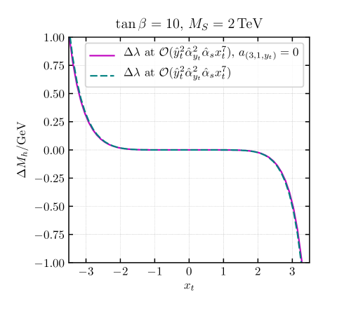
Figure 1: Impact on the Higgs mass from 3-loop threshold correction $\Delta\lambda$ from the highest power $x_{t}$ contribution at $\mathcal{O}(\hat{y}_{t}^{6}\hat{g}_{3}^{2})$. The values of the Higgs mass are obtained by the calculation implemented in ref. Kwasnitza:2020wli and its modifications.

In figure 1 we compare the Higgs mass as predicted by the unmodified FlexibleEFTHiggs calculation (with $a_{(3,1,y_{t})}=0$) and the version with the correct term from eq. (61) for a characteristic SUSY scale $M_{S}=2\,$TeV. From both calculations we subtracted the result obtained by the version where the high-scale correction $\mathcal{O}(\hat{y}_{t}^{6}\hat{g}_{3}^{2}x_{t}^{7})$ is set to zero. The dashed line thus shows the impact of the complete threshold correction eq. (61) on the Higgs mass. The solid line represents the impact of the incomplete threshold correction in the implementation of ref. Kwasnitza:2020wli , where the 2-loop coefficient $a_{(3,1,y_{t})}=0$. In the considered limit the threshold correction is important and $\Delta M_{h}\approx 500\,$MeV for $x_{t}\approx 3$. But the difference between the complete and incomplete version, i.e. of the contribution of $a_{(3,1,y_{t})}$ to the threshold correction in $\hat{\lambda}^{\text{SM}}$ is negligible.

Hence, although the Higgs mass calculation implemented in ref. Kwasnitza:2020wli does not contain a 2-loop threshold to the Yukawa matching at $\mathcal{O}(y_{t}^{3}g_{3}^{2})$, it therefore reproduces the 3-loop term $\hat{y}_{t}^{6}\hat{g}_{3}^{2}x_{t}^{7}\subset\hat{\lambda}^{\text{SM}}$ to a very good numerical precision.

$\hat{\lambda}^{\text{SM}}$ at $\hat{y}_{b}^{4}\hat{y}_{t}^{2l}(A_{t}/M_{S})^{l}(\tan\beta)^{4+l}$:

Now we discuss these mixed Yukawa expressions which are beyond the terms listed in table 2, as they do not contain any QCD coupling $g_{3}$. This analysis is in line with the resummation of $\mathcal{O}(\hat{y}_{b}(\hat{y}_{t}^{2}A_{t}\tan\beta/M_{S})^{l})$ in the MSSM bottom Yukawa coupling presented in ref. Noth:2008tw ; Noth:2010jy . Here we derive a simultaneous resummation of these terms in $\Delta y_{b}^{\text{SM}}$ and $\hat{\lambda}^{\text{SM}}$. It is sufficient in our analysis to include the following 1-loop thresholds corrections

$$\Delta\lambda \supset(y_{b}c_{\beta})^{4}c_{(4,0,y_{b})}x_{b}^{4},$$ (62a)

$$\Delta y_{b} \supset(y_{b}c_{\beta})y_{t}^{2}a_{(b,t)}x_{t}\tan\beta,$$ (62b)

where $a_{(b,t)}$ and $c_{(4,0,y_{b})}$ are independent of $x_{q}$ and $\tan\beta$. Following the reparametrization prescription of eq. (49), the included corrections to $\hat{\lambda}^{\text{SM}}$ are

$$\left.\hat{\lambda}^{\text{SM}}\right|_{\hat{y}_{b}^{4}\hat{y}_{t}^{2l}x_{t}^{l}x_{b}^{4}\tan^{l}\beta}=\hat{y}_{b}^{4}\frac{c_{(4,0,y_{b})}}{\left[1+\frac{\hat{y}_{t}^{2}}{s_{\beta}^{2}}a_{(b,t)}x_{t}\tan\beta\right]^{4}}x_{b}^{4}\,.$$ (63)

Expressed in terms of $A_{t}$ and $\tan\beta$, the terms in (63) are of $\mathcal{O}(\hat{y}_{b}^{4}\hat{y}_{t}^{2l}(A_{t}/M_{S})^{l}(\tan\beta)^{4+l})$. In consequence, eq. (63) resums terms leading in powers of $(A_{t}\tan\beta/M_{S})$.

Now we argue why no explicit multi-loop contributions to eq. (62) exist which may affect the terms in eq. (63). As discussed in the items of section 4.1, the only mechanism to introduce contributions $\propto\tan\beta$ at $\mathcal{O}(y_{b}^{4}y_{t}^{2k})$ is through the sbottom-mixing parameter $x_{b}$. In order to give rise to corrections to eq. (63), the diagrams would be of $\mathcal{O}(y_{b}^{4}x_{b}^{k+4}y_{t}^{2k}x_{t}^{k})$, for $k>1$. But as stated in section 2.3, the analysis in section 2.1 forbids such (unsuppressed) terms explicitly, because the $x_{b}$ parameter cannot appear with higher powers than $y_{b}$.

We note in passing, that the resummation covers terms as $x_{b}^{4+l}x_{t}^{l}$ but not $x_{b}^{4}x_{t}^{2l}$, where the same overall power in $x_{q}$ is distributed differently among $x_{t,b}$. Clearly, for $\tan\beta\gg x_{t}$ the resummed terms in eq. (63), at $\mathcal{O}(\hat{y}_{b}^{4}\hat{y}_{t}^{2l})$ are dominant.

Resummation of flavor violating stop-scharm-Higgs soft parameter in $\hat{\lambda}^{\text{SM}}$

As announced in the comments of section 2.3 there exist constraints for flavor-violating trilinear parameters. Now we use such a constraint to derive a resummation of stop-scharm-Higgs couplings, which are not listed in table 2 as they are not associated to the third generation only. In the style of eq. (52), we present an all-order equation of enhanced flavor violating contributions from soft-breaking $A$-terms.

The impact of mixing effects between the second and third generation of squarks onto the Higgs mass has been studied for example in refs. Heinemeyer:2004by ; Heinemeyer:2004gx ; AranaCatania:2011ak ; Arana-Catania:2014ooa at 1-loop and in ref. Goodsell:2015yca at 2-loop. It was shown that among all sources of flavor violation the trilinear chirality changing interactions can particularly contribute to the Higgs mass without being in conflict with other observables.

In this section we work in the weak basis for quarks and squarks and with mass eigenstates of the scalar Higgs sector. The interaction of interest is induced by the (real) soft SUSY-breaking trilinear coupling

$$\mathcal{L}^{\text{soft}}\supset-\frac{T_{23}^{u}s_{\beta}}{\sqrt{2}}\,h\,\tilde{c}_{L}^{\dagger}\tilde{t}_{R}^{\phantom{\dagger}}-\frac{T_{32}^{u}s_{\beta}}{\sqrt{2}}\,h\,\tilde{t}_{L}^{\dagger}\tilde{c}_{R}^{\phantom{\dagger}}+-\frac{T_{33}^{u}s_{\beta}}{\sqrt{2}}\,h\,\tilde{t}_{L}^{\dagger}\tilde{t}_{R}^{\phantom{\dagger}}+\text{h.c.}~{},$$ (64)

where we decompose the $T^{u}_{ij}$ coupling in a product of the ($i$,$j$) entries of the up-type Yukawa ($3\times 3$)-matrix $y^{u}_{ij}$ and of the $M_{S}$-enhanced matrix $A^{u}_{ij}$, i.e. $T_{ij}^{u}=y_{ij}^{u}A_{ij}^{u}$.

In the following we elaborate how a 1-loop analysis allows for the inclusion of contributions which are of highest power in $(A_{23}^{u}A_{33}^{u}/M_{S}^{2})$ in leading QCD order. We consider matching of Green functions $\Gamma_{\bar{t}th}$, $\Gamma_{\bar{t}ch}$ and $\Gamma_{h^{4}}$, where the external quarks $c$ and $t$ are the up-type quarks of the second and third generation defined in the weak basis. Analogous to eq. (10) the matching results in a relation of the Yukawa couplings in the SM and MSSM which is expanded in loops, $\hat{y}^{u}_{ij}=s_{\beta}y^{u}_{ij}+\Delta y^{u}_{ij}$. As in eq. (51), 1-loop threshold corrections for the Yukawa couplings $\hat{y}_{33}^{u}$, $\hat{y}_{23}^{u}$ and the quartic $\hat{\lambda}$ include enhancements by the trilinear parameters $A_{ij}^{u}$. We focus on 1-loop contributions which contain $A_{33}^{u}/M_{S}$ and $A_{23}^{u}/M_{S}$

$$\left.\Delta y^{u}_{33}\right|_{A^{u}_{33}} =s_{\beta}y_{33}^{u}g_{3}^{2}a_{(\tilde{t},\tilde{t})}\frac{A_{33}^{u}}{M_{S}}\supset\leavevmode\hbox to112.71pt{\vbox to64.96pt{\text{[drawing]}}}+\cdots\,, t \tilde{t}_{R} \tilde{t}_{L} t \tilde{g} h t \tilde{t}_{R} \tilde{t}_{L} t \tilde{g} h$$ (65)

$$\left.\Delta y^{u}_{23}\right|_{A^{u}_{23}} =s_{\beta}y_{23}^{u}g_{3}^{2}a_{(\tilde{t},\tilde{c})}\frac{A_{23}^{u}}{M_{S}}\supset\leavevmode\hbox to113.07pt{\vbox to64.96pt{\text{[drawing]}}}+\cdots\,, t \tilde{t}_{R} \tilde{c}_{L} c \tilde{g} h t \tilde{t}_{R} \tilde{c}_{L} c \tilde{g} h$$ (66)

$$\left.\Delta\lambda\right|_{(A_{33}^{u}A^{u}_{23})^{2}} =s_{\beta}^{4}(y^{u}_{33}\,y^{u}_{23})^{2}c_{(\tilde{t},\tilde{c})}\left(\frac{A^{u}_{33}A^{u}_{23}}{M_{S}^{2}}\right)^{2}\supset\leavevmode\hbox to112.01pt{\vbox to84.74pt{\text{[drawing]}}}+\cdots, h h \tilde{t}_{R} \tilde{t}_{L} h h \tilde{t}_{R} \tilde{c}_{L} h h \tilde{t}_{R} \tilde{t}_{L} h h \tilde{t}_{R} \tilde{c}_{L}$$ (67)

where the coefficients $a_{(...)}$ and $c_{(...)}$ are independent of $A_{ij}^{u}$ and $\beta$. Solving the matching equation for the MSSM coupling $y_{ij}^{u}$, including 1-loop corrections from eqs. (65,66), results in a power series in $(g_{3}^{2n}(A_{33}^{u},A_{23}^{u})^{n})$. In consequence, the expansion of $\Delta\lambda$ in eq. (67) in terms of SM couplings leads to a series of (unsuppressed) highest power contributions in $A_{33}^{u}$ and $A_{23}^{u}$

$$\left.\hat{\lambda}^{\text{SM}}\right|_{(\hat{y}_{33}^{u}\hat{y}_{23}^{u})^{2}\hat{g}_{3}^{2l}} =(\hat{y}_{33}^{u}\,\hat{y}_{23}^{u})^{2}\left(\frac{A_{33}^{u}A_{23}^{u}}{M_{S}^{2}}\right)^{2}\frac{c_{(\tilde{t},\tilde{c})}}{\left[1+\hat{g}_{3}^{2}a_{(\tilde{t},\tilde{t})}\frac{A_{33}^{u}}{M_{S}}\right]^{2}\left[1+\hat{g}_{3}^{2}a_{(\tilde{t},\tilde{c})}\frac{A_{23}^{u}}{M_{S}}\right]^{2}}.$$ (68)

Now we ask if there exist explicit multi-loop corrections to $\Delta\lambda$ or to $\Delta y_{ij}^{u}$ (in full-model parametrization) which modify terms in eq. (68) (EFT-parametrization). Indeed, as in all previous cases we can apply the arguments given in section 2.2 and conclude that the power of $A_{ij}$ is maximally the power of the Yukawa coupling $y_{ij}$ in the threshold correction:

In full-model parametrization, the highest power contributions to threshold corrections $\Delta\lambda$ and $\Delta y_{ij}^{u}$ are of order $\mathcal{O}(g_{3}^{2n}(y_{33}^{u}A_{33}^{u}/M_{S})^{n_{t}}(y_{23}^{u}A_{23}^{u}/M_{S})^{n_{tc}})$, for all positive integers $n$, $n_{t},n_{tc}>0$.
This means that terms in eq. (68) do not receive any corrections from higher orders and are resummed.

Similar conclusions apply for contributions to $\hat{\lambda}^{\text{SM}}$ with no $\hat{y}^{u}_{33}$ enhancement and more powers in $\hat{y}_{23}^{u}$, i.e the inclusion of 1-loop contributions $\mathcal{O}((y_{23}^{u}A_{23}^{u})^{4})$ to $\Delta\lambda$ results in a resummation of $\mathcal{O}((\hat{y}_{23}^{u})^{4}\hat{g}_{3}^{2l}(A_{23}^{u}/M_{S})^{l+4})$ in $\hat{\lambda}^{\text{SM}}$. Clearly, the discussion of the $A_{32}^{u}$ coupling is identical.

4.3 What cannot be resummed

So far we have mainly focused on the resummation of QCD-enhanced terms $\hat{g}_{3}^{2n}x_{q}^{n}$. Now we discuss, whether it is possible to resum terms $\propto\hat{y}_{q}^{2n}x_{q}^{2n}$, where the powers of $x_{q}$ are related to the powers of Yukawa couplings. Such terms are of particular interest, since at a given loop order they are of higher power in $x_{q}$ than the $g_{3}$-enhanced terms. The answer is no. As derived in section 2.2, the maximal power of $x_{q}$ (unsuppressed) in explicit contributions to threshold corrections is given by the power of Yukawa couplings $y_{q}$. Thus, the reparametrization of threshold corrections in terms of EFT couplings alone cannot completely capture highest-power terms of $\mathcal{O}((\hat{y}_{t}x_{t})^{n_{t}}(\hat{y}_{b}x_{b})^{n_{b}})$. If no other restrictions are invoked, our analysis has implications on the limits of reorganizing the perturbative expansion:

• one cannot resum $\mathcal{O}((\hat{y}_{t}x_{t})^{n_{t}}(\hat{y}_{b}x_{b})^{n_{b}})$ in corrections $\Delta y_{q}^{\text{SM}}$,

• one cannot resum $\mathcal{O}((\hat{y}_{t}x_{t})^{n_{t}}(\hat{y}_{b}x_{b})^{n_{b}})$ in corrections $\hat{\lambda}^{\text{SM}}$.

Note that the discussion around eq. (63) leads to a resummation for pure Yukawa orders unrelated to QCD, which is consistent with the given remarks.

5 Conclusions

In this paper we established all-order statements on the appearance of the parameters $x_{q}$ in MSSM Green functions and threshold corrections between MSSM and SM couplings in the context of minimal subtraction schemes $\overline{\text{DR}}$ and $\overline{\text{MS}}$. We focused particularly on the quartic Higgs coupling $\lambda$. The optimum setting for the statements is full-model parametrization, i.e. perturbative expansion in terms of MSSM couplings including, if needed, truncation of the expansion at fixed order in terms of these couplings.

In full-model parametrization our first main statements are constraints on the threshold corrections $\Delta y_{q}$ and $\Delta\lambda$, see eqs. (12) and (14), stating which powers in the $x_{q}$ parameters are forbidden. These statements generalize results from the literature focusing on constraints for powers of $\tan\beta$ in $\Delta y_{b}$ Carena:1999py ; Noth:2008 . Our second set of statements are constraints on powers of $x_{q}$ in the Green functions $\Gamma_{\bar{q}qh}$ and $\Gamma_{h^{4}}$, see eqs. (25) and (27). These constraints are weaker than the ones on threshold corrections; the higher-power $x_{q}$ contributions to the Green functions originate from an integration region where the internal loop momenta are soft. The consistency of the constraints on $\Delta\lambda$ and $\Gamma_{h^{4}}$ has been illustrated by an explicit matching calculation of $\Gamma_{h^{4}}$ in the broken phase in section 3.2. There the cancellation of powers $x_{q}^{\geq 4}$ contributions at $\mathcal{O}(y_{q}^{4}g_{3}^{10})$ was explicitly demonstrated.

We remark that the constraints presented here are specific to minimal subtraction schemes. For example, the appearance of $x_{q}^{n}$-terms in Green-functions renormalized in the on-shell scheme is different, see e.g. Noth:2008 .

One practical relevance of the threshold constraints is that they often lead to an effective resummation of (sub-)leading $x_{q}$-contributions: Many calculations are done in a context where the Yukawa couplings are fixed by low-scale parameters. This requires the full-model Yukawa coupling $y_{q}$ to be determined in terms of the EFT coupling $\hat{y}_{q}$. This procedure inverts and combines fixed-order relations and thereby generates terms of higher orders in loops and in $x_{q}$. Using the derived constraints one can prove that certain towers of terms are actually correct, i.e. “resummed” at all orders. In section 4.1 we gave a general description of the towers of the resummed terms in $x_{q}$, or in the context of related parameters such as $A_{q}$ and $\tan\beta$. As a special case we identified that the well-known $\tan\beta$-resummation in the bottom Yukawa coupling works analogously for $\hat{\lambda}$ and therefore for the Higgs mass. In section 4.2 we explored a plethora of multi-loop structures which are subject to this parameter resummation. We gave analytic expressions for all-order contributions to $\hat{\lambda}$ for the dominant parameter-enhanced terms, i.e. (sub)leading powers of $\tan\beta,~{}A_{q}$ or $x_{q}$.

Here we summarize the relevant properties why this resummation of highest power terms in the BSM parameter $x_{q}$ is possible.

• Matching in full-model parametrization: The matching of Green functions at a fixed order yields threshold corrections where each factor of $x_{q}$ is necessarily accommodated by a factor of full-model Yukawa coupling $y_{q}$.

• Decoupling of $y_{q}$ and $x_{q}$ through reparametrization: The threshold corrections are then reparametrized in terms of EFT parameters. Because of the structure of the Yukawa matching, reparametrizing decouples the maximal power of $x_{q}$ from the power in the EFT Yukawa coupling $\hat{y}_{q}$. As a result the threshold corrections contain terms of $\mathcal{O}(\hat{y}_{q}(\hat{g}_{3}^{2}x_{q})^{n})$, i.e. terms where each additional order in $g_{3}^{2}$ is accompanied by a factor of $x_{q}$.

• Correctness of the reparametrization terms with higher power in $x_{q}$: By following the arguments given in section 2.2 (or in section 3.1), one can check that such terms, which are leading or subleading in $x_{q}$, are correctly “resummed” for any $n$, even though they are generated from a fixed-order calculation via reparametrization.

Clearly, similar analyses may be carried out for other BSM parameters if similar properties apply.

6 Acknowledgments

We are grateful to Alexander Voigt for discussions on applications of our results, and to Ulrich Nierste for detailed discussions of $\tan\beta$-resummation and of refs. Carena:1999py ; Hofer:2009xb . This research was supported by the German Research Foundation (DFG) under grant number STO 876/2-2 and by the high-performance computing cluster Taurus at ZIH, TU Dresden.

Appendix A Leading contributions from LME and effective vertices

In this appendix we list the effective vertices appearing in a large mass expansion (LME) of diagrams with at least one heavy internal propagator. First, we analyze the relevant Higgs-fermion interactions which lead to non-trivial $x_{q}$ contributions. Second, we discuss gluon interactions by invoking arguments from $SU(3)_{C}$ BRST invariance. We are interested in vertices which have a non-negative mass dimension and no $v/M_{S}$-suppression. Thus, the selection of effective vertices we have to inspect is finite. We further focus on contributions with minimal powers in the Yukawa coupling and maximal powers in the QCD gauge coupling. For such contributions we inspect the highest power $x_{q}$ contributions which are unsuppressed i.e. $\propto(v/M_{S})^{0}$.

A.1 Effective vertices with fermions and the quartic interaction of Higgs bosons

The procedure of a LME naturally produces the structure of an EFT. The effective vertices arise from applying Taylor operations on one-light-particle irreducible (1LPI) diagrams. Here we carry out a dimensional analysis of the effective vertices arising in this way, with focus on the appearance of $x_{q}$. Symbolically our notation of the expressions is given as

$$\begin{split}\mathcal{T}_{\left\{m,p\right\}}\left\{\leavevmode\hbox to89.09pt{\vbox to68.28pt{\text{[drawing]}}}\right\}{=}&\leavevmode\hbox to89.09pt{\vbox to68.28pt{\text{[drawing]}}}\equiv\Delta v_{l^{4}}\supset x_{q}^{\leq j}~{},\end{split} l l l l l l l l l l l l l l l l$$ (69)

where the blob on the left-hand side denotes a 1LPI Green function with light external fields $l$ of mass scale $m$ and with external momenta $p$. The symbol $\mathcal{T}$ denotes the Taylor operator with respect to the indicated variables, which by definition acts on the Feynman integrand. On the right-hand side, $\Delta v_{l^{4}}$ represents the effective vertex, which is a power series in $1/M_{S}$. Furthermore, in eq. (69) the notation “$\Delta v\supset x_{q}^{\leq j}$” specifies that only terms with $x_{q}^{\leq j}$ appear in the effective vertex, while terms with $x_{q}^{>j}$ are absent.

As outlined in section 2, the diagrammatic contributions enhanced by the squark mixing parameter $x_{q}$ arise in two ways:

• by the trilinear coupling of the Higgs bosons with the left- and right-handed squarks in eq. (4) which is accompanied by a factor of the Yukawa coupling

• by the chirality flip vertex, induced by the off-diagonal entry in the squark-mass matrix eq. (7), which is accompanied by a factor of quark mass $m_{q}\propto m$ and the scale $M_{S}$.

At leading QCD order there are no internal vertices with a Yukawa coupling and hence no internal Higgs boson propagators. Therefore, trilinear squark-Higgs vertices are only possible at couplings with the external Higgs lines, and the number of possible $x_{q}$ enhanced trilinear vertices is bounded by the number of external Higgs lines associated with the effective vertex $\Delta v$. In stark contrast, the chirality flip vertex in the internal squark propagator could be inserted arbitrarily often at any fixed loop order. Nonetheless, dimensional analysis can be applied in order to establish a relation between the number of chirality flips and the power of the mass suppression factor $m/M_{S}$ as follows.

For the detailed analysis we fix $\Delta v$ to be an effective vertex with $n_{h}$ external Higgs boson lines of mass dimension $n_{d}$, i.e. ${\left[\Delta v\right]=\left[\text{mass}\right]^{n_{d}}}$. Furthermore, we allow for $n_{I}$ chirality flip insertions in the squark lines. For this case, the highest-power $x_{q}$ contribution to the effective vertex is given by

$$\Delta v\supset \left({y_{q}}x_{q}M_{S}\right)^{n_{h}}\left(mM_{S}x_{q}\right)^{n_{I}}\int_{k}\mathcal{T}_{\left\{m,p\right\}}f(m,p,M_{S},k)~{},$$ (70)

where the common appearances of $x_{q}$ and the Yukawa coupling, the mass $m$ and $M_{S}$ has been made explicit. The evaluation of the leading term in the Taylor expansion leads to a loop integral function which depends on the physical scale $M_{S}$ only

$$\Delta v\supset \left({y_{q}}x_{q}M_{S}\right)^{n_{h}}\left(mM_{S}x_{q}\right)^{n_{I}}p^{n_{p}}I(M_{S})\left[\text{const}+\mathcal{O}\left(\frac{m,p}{M_{S}}\right)\right],$$ (71)

$$= ({y_{q}}x_{q})^{n_{h}}(x_{q}m)^{n_{d}-n_{p}}p^{n_{p}}\left(x_{q}\frac{m}{M_{S}}\right)^{n_{I}+n_{p}-n_{d}}\left[\text{const}+\mathcal{O}\left(\frac{m,p}{M_{S}}\right)\right],$$ (72)

where $n_{p}$ represents the minimum power in the external momentum $p$ required for the effective vertex (the precise Lorentz structure of the effective vertex can be ignored and is not specified). In the last equation we used the fact that $\Delta v$ is of mass dimension $[\text{mass}]^{n_{d}}$. For ${n_{d}}>n_{I}$ the dimensional analysis does not forbid contributions to the effective vertex with positive powers in $M_{S}$.

The previous equations elucidate that for a fixed vertex function (with fixed $n_{h}$, $n_{d}$, $n_{p}$), each additional internal squark chirality flip results in an additional mass suppression factor $m/M_{S}$. For the especially interesting case $n_{p}=0$, the maximal power of $x_{q}$ without mass suppression is realized for ${n_{d}}=n_{I}$, and this maximal power is $x_{q}^{n_{d}+n_{h}}\subset\Delta v$.

Eq. (70) implies that a product of effective vertices $\Pi_{i=1}^{n}\Delta v_{i}$ behaves the same way as the expression on the r.h.s. of eq. (72), i.e. the product of effective vertices can be expressed with indices $n_{h}^{\prime}$, $n_{I}^{\prime}$ and $n_{d}^{\prime}$ obtained from the respective sum of the indices $(n_{h})_{i}$, $(n_{I})_{i}$ and $(n_{d})_{i}$ of the individual effective vertices $\Delta v_{i}$.

We note that the reasoning does not depend on the number of fermions coupled to Higgs bosons by the effective vertex $\Delta v$. Furthermore, the arguments are also independent of the specific order in the QCD coupling $g_{3}$.

In the following we list the results from analyzing diagrammatic contributions with non-negative mass dimension by this procedure. The following results thus correspond to explicit versions of eq. (72), specialized to these vertices. On the r.h.s. we always specify only the leading terms and suppress possible factors $\left[\text{const}+\mathcal{O}\left(\frac{m,p}{M_{S}}\right)\right]$. As in sec. 3 we will denote effective vertices which contain unsuppressed $x_{q}$ contributions by gray squares. In contrast, effective vertices without $x_{q}$ enhancement are represented by white squares.

(1) effective Higgs-quark vertex $$\Delta v_{\bar{q}qh}$$:

(74)

(2) effective quark propagator insertion $$\Delta v_{\bar{q}q}$$:

$$\begin{split}\leavevmode\hbox to66.13pt{\vbox to21.17pt{\text{[drawing]}}}&\equiv\Delta v_{\bar{q}q}=\Delta v_{m}+\Delta v_{\not{p}}\end{split} q q q q$$ (75)

$$\quad~{}\Delta v_{m}\supset g_{3}^{2k}\,m\,x_{q}^{\leq 1}\left(x_{q}\frac{m}{M_{S}}\right)^{n_{I}-1}$$ (76)

$$\quad~{}\Delta v_{\not{p}}\supset g_{3}^{2k}\,\not{p}\,x_{q}^{0}\left(x_{q}\frac{m}{M_{S}}\right)^{n_{I}}$$ (77)

(3) effective quartic Higgs vertex $$\Delta v_{h^{4}}$$:

(79)

(4) effective gluon-quark vertex $$\Delta v_{g\bar{q}q}$$:

$$\begin{split}\leavevmode\hbox to63pt{\vbox to37.96pt{\text{[drawing]}}}&\supset g_{3}^{2k+1}x_{q}^{0}\left[\gamma^{\mu}+\mathcal{O}\left(\frac{p^{\mu},m\gamma^{\mu}}{M_{S}}\right)\right]\left(x_{q}\frac{m}{M_{S}}\right)^{n_{I}}.\end{split} q q g q q g$$ (80)

(5) effective vertex for gluon interactions $$\Delta v_{g^{3}} \Delta v_{g^{4}} x_{q}$$ and : By covariant decomposition and dimensional analysis it follows that enhanced contributions are suppressed as

(81)

(82)

A.2 Effective vertices with gluons, ghosts and Higgs bosons

For the following effective vertices involving external gluons and Higgs bosons, we extend the reasoning by arguments based on BRST invariance and its consequences. To exemplify why this is helpful, we consider a diagrammatic contribution to the gluon propagator $\Gamma_{gg}$. Based on a Taylor expansion (at leading order) and dimensional analysis one might evaluate individual diagrams as

(83)

where the $\cal T$ denotes that the corresponding loop integrand is Taylor expanded in $m$ and $p$. The leading term in the LME absorbs UV contributions from heavy fields ($M_{S}\gg m$) in the effective vertices of light fields present in the EFT. Thus, the effective vertex can be regarded as a construction of decoupling coefficients of operators in the EFT Lagrangian of the SM which in turn is invariant under $SU(3)_{C}$ BRST transformations.

Individual diagrams indeed behave in the way shown in eq. (83). However, after the inclusion of all diagrams to $\Gamma_{gg}$ the entire contribution has to be proportional to the transverse projector $T^{\mu\nu}\propto p^{\mu}p^{\nu}-p^{2}\eta^{\mu\nu}$. Relying on the existence of a BRST invariant EFT implies transversality also after Taylor expansion, i.e. the full result in eq. (83) is independent of the $(M_{S}+m)^{2}$ term at each order,

$$\sum\limits_{\text{heavy lines}\geq 1}\leavevmode\hbox to87.47pt{\vbox to29.42pt{\text{[drawing]}}} g g \mathcal{T} g g \mathcal{T} \overset{\phantom{\text{LME}}}{\equiv}\leavevmode\hbox to60.15pt{\vbox to18.19pt{\text{[drawing]}}}\propto g_{3}^{2k}T^{\mu\nu}. g g g g$$ (84)

In the following we continue our list of effective vertices. In each case we now assume a summation over all contributing diagrams to ensure the cancellation of spurious contributions analogous to the ones on the r.h.s. in eq. (83).

(6) gluon-gluon effective vertex $$\Delta v_{gg} n_{p}\geq 2 x_{q}$$ : Having discussed the transverse structure of the effective vertex, we can link the contributions in eq. (84) to the master formula in eq. (72). In that formula the transversality now implies the momentum dependence , and as a result the appearance can be characterized as

(86)

(7) effective Higgs-gluon vertex $$\Delta v_{ggh} \Delta v_{gghh} n_{p}\geq 2$$ and : The Higgs-gluon interactions can be associated to dimension 6 (or higher) operators in the corresponding EFT and as before we obtain in eq. (72). Therefore, these effective interactions are constrained as follows,

(87)

(88)

where $$(p^{2})^{\mu\nu} M_{S}$$ represents a vertex-dependent bilinear combination of the external momenta. Importantly, both contributions are suppressed by large .

(8) effective ghost-antighost vertex $$\Delta v_{\bar{c}c} \Delta v_{\bar{c}c} p^{2} x_{q}$$: The effective vertices involving ghosts can be discussed in a similar way. Due to BRST invariance, the effective QCD ghost-antighost vertex obeys a proportionality to the squared external momentum , resulting in suppressed -enhanced contributions

(89)

(9) effective ghost-gluon vertex $$\Delta v_{g\bar{c}c}$$: This effective vertex can be directly evaluated by covariant decomposition and dimensional analysis as

(90)

There are further QCD related interactions, trilinear and quartic, involving Higgs, ghosts and gluons, which we do not list. Because of BRST invariance such interactions are associated with higher dimensional operators in the EFT and are necessarily suppressed at least by a factor of $p/M_{S}$.

In summary, using eq. (72) we have established the properties that are necessary for classification of eqs. (32,33,34):

• The crucial behavior of the effective vertices in eq. (32) is characterized by ${n_{d}<0}$. Eq. (72) implies, irrespectively of the specific $x_{q}$ appearance, that any contribution is suppressed at least by a factor of $v/M_{S}$.

• The effective vertices in eq. (33) are described by $n_{d}=n_{p}$ and $n_{h}=0$. Therefore, no positive $x_{q}$ power can originate at $\mathcal{O}((v/M_{S})^{0})$.

• The central effective vertices in eq. (34) which introduce positive powers of $x_{q}$ arise in two ways. On the one hand the two-quark vertex in eq. (76) has the property $n_{d}>n_{p}$ and on the other hand the effective vertices in eqs. (LABEL:eq:eff_vert_qqh,LABEL:eq:eff_vert_hhhh) feature $n_{h}\geq 0$ and $n_{d}=n_{p}$.

References

- (1) ATLAS, CMS collaboration, G. Aad et al., Combined Measurement of the Higgs Boson Mass in Collisions at and 8 TeV with the ATLAS and CMS Experiments, Phys. Rev. Lett. 114 (2015) 191803, [1503.07589].
- (2) Particle Data Group collaboration, M. Tanabashi et al., Review of Particle Physics, Phys. Rev. D98 (2018) 030001.
- (3) P. Draper, G. Lee and C. E. M. Wagner, Precise estimates of the Higgs mass in heavy supersymmetry, Phys. Rev. D89 (2014) 055023, [1312.5743].
- (4) E. Bagnaschi, G. F. Giudice, P. Slavich and A. Strumia, Higgs Mass and Unnatural Supersymmetry, JHEP 09 (2014) 092, [1407.4081].
- (5) J. Pardo Vega and G. Villadoro, SusyHD: Higgs mass Determination in Supersymmetry, JHEP 07 (2015) 159, [1504.05200].
- (6) G. Lee and C. E. M. Wagner, Higgs bosons in heavy supersymmetry with an intermediate mA, Phys. Rev. D92 (2015) 075032, [1508.00576].
- (7) E. Bagnaschi, J. Pardo Vega and P. Slavich, Improved determination of the Higgs mass in the MSSM with heavy superpartners, Eur. Phys. J. C77 (2017) 334, [1703.08166].
- (8) J. Braathen, M. D. Goodsell and P. Slavich, Matching renormalisable couplings: simple schemes and a plot, Eur. Phys. J. C79 (2019) 669, [1810.09388].
- (9) M. Gabelmann, M. Mühlleitner and F. Staub, Automatised matching between two scalar sectors at the one-loop level, Eur. Phys. J. C79 (2019) 163, [1810.12326].
- (10) B. C. Allanach and A. Voigt, Uncertainties in the Lightest Even Higgs Boson Mass Prediction in the Minimal Supersymmetric Standard Model: Fixed Order Versus Effective Field Theory Prediction, Eur. Phys. J. C78 (2018) 573, [1804.09410].
- (11) R. V. Harlander, J. Klappert, A. D. Ochoa Franco and A. Voigt, The light CP-even MSSM Higgs mass resummed to fourth logarithmic order, Eur. Phys. J. C78 (2018) 874, [1807.03509].
- (12) E. Bagnaschi, G. Degrassi, S. Paßehr and P. Slavich, Full two-loop QCD corrections to the Higgs mass in the MSSM with heavy superpartners, 1908.01670.
- (13) M. Krämer, B. Summ and A. Voigt, Completing the scalar and fermionic Universal One-Loop Effective Action, JHEP 01 (2020) 079, [1908.04798].
- (14) H. Bahl, I. Sobolev and G. Weiglein, Precise prediction for the mass of the light MSSM Higgs boson for the case of a heavy gluino, 1912.10002.
- (15) T. Hahn, S. Heinemeyer, W. Hollik, H. Rzehak and G. Weiglein, High-Precision Predictions for the Light CP -Even Higgs Boson Mass of the Minimal Supersymmetric Standard Model, Phys. Rev. Lett. 112 (2014) 141801, [1312.4937].
- (16) H. Bahl and W. Hollik, Precise prediction for the light MSSM Higgs boson mass combining effective field theory and fixed-order calculations, Eur. Phys. J. C76 (2016) 499, [1608.01880].
- (17) P. Athron, J.-h. Park, T. Steudtner, D. Stöckinger and A. Voigt, Precise Higgs mass calculations in (non-)minimal supersymmetry at both high and low scales, JHEP 01 (2017) 079, [1609.00371].
- (18) F. Staub and W. Porod, Improved predictions for intermediate and heavy Supersymmetry in the MSSM and beyond, 1703.03267.
- (19) P. Athron, M. Bach, D. Harries, T. Kwasnitza, J.-h. Park, D. Stöckinger et al., FlexibleSUSY 2.0: Extensions to investigate the phenomenology of SUSY and non-SUSY models, Comput. Phys. Commun. 230 (2018) 145–217, [1710.03760].
- (20) H. Bahl, S. Heinemeyer, W. Hollik and G. Weiglein, Reconciling EFT and hybrid calculations of the light MSSM Higgs-boson mass, 1706.00346.
- (21) H. Bahl and W. Hollik, Precise prediction of the MSSM Higgs boson masses for low MA, JHEP 07 (2018) 182, [1805.00867].
- (22) E. A. Reyes R. and A. R. Fazio, Comparison of the EFT Hybrid and Three-Loop Fixed-Order Calculations of the Lightest MSSM Higgs Boson Mass, Phys. Rev. D100 (2019) 115017, [1908.00693].
- (23) R. V. Harlander, J. Klappert and A. Voigt, The light CP-even MSSM Higgs mass including N3LO+N3LL QCD corrections, Eur. Phys. J. C80 (2020) 186, [1910.03595].
- (24) H. Bahl, S. Heinemeyer, W. Hollik and G. Weiglein, Theoretical uncertainties in the MSSM Higgs boson mass calculation, 1912.04199.
- (25) T. Kwasnitza, D. Stöckinger and A. Voigt, Improved MSSM Higgs mass calculation using the 3-loop FlexibleEFTHiggs approach including -resummation, 2003.04639.
- (26) H. Bahl, I. Sobolev and G. Weiglein, The light MSSM Higgs boson mass for large and complex input parameters, Eur. Phys. J. C 80 (2020) 1063, [2009.07572].
- (27) P. Draper and H. Rzehak, A Review of Higgs Mass Calculations in Supersymmetric Models, Phys. Rept. 619 (2016) 1–24, [1601.01890].
- (28) P. Slavich et al., Higgs-mass predictions in the MSSM and beyond, 2012.15629.
- (29) M. Carena, D. Garcia, U. Nierste and C. E. M. Wagner, Effective Lagrangian for the interaction in the MSSM and charged Higgs phenomenology, Nucl. Phys. B577 (2000) 88–120, [hep-ph/9912516].
- (30) J. Guasch, P. Hafliger and M. Spira, MSSM Higgs decays to bottom quark pairs revisited, Phys. Rev. D 68 (2003) 115001, [hep-ph/0305101].
- (31) L. Hofer, U. Nierste and D. Scherer, Resummation of tan-beta-enhanced supersymmetric loop corrections beyond the decoupling limit, JHEP 10 (2009) 081, [0907.5408].
- (32) D. Noth and M. Spira, Higgs Boson Couplings to Bottom Quarks: Two-Loop Supersymmetry-QCD Corrections, Phys. Rev. Lett. 101 (2008) 181801, [0808.0087].
- (33) D. Noth and M. Spira, Supersymmetric Higgs Yukawa Couplings to Bottom Quarks at next-to-next-to-leading Order, JHEP 06 (2011) 084, [1001.1935].
- (34) S. Marchetti, S. Mertens, U. Nierste and D. Stockinger, Tan(beta)-enhanced supersymmetric corrections to the anomalous magnetic moment of the muon, Phys. Rev. D 79 (2009) 013010, [0808.1530].
- (35) J. R. Espinosa and R.-J. Zhang, Complete two loop dominant corrections to the mass of the lightest CP even Higgs boson in the minimal supersymmetric standard model, Nucl. Phys. B586 (2000) 3–38, [hep-ph/0003246].
- (36) T. Kinoshita, Mass singularities of Feynman amplitudes, J. Math. Phys. 3 (1962) 650–677.
- (37) T. Lee and M. Nauenberg, Degenerate Systems and Mass Singularities, Phys. Rev. 133 (1964) B1549–B1562.
- (38) G. F. Sterman, Kinoshita’s Theorem in Yang-Mills Theories, Phys. Rev. D 14 (1976) 2123–2125.
- (39) A. V. Bednyakov, Running mass of the b-quark in QCD and SUSY QCD, Int. J. Mod. Phys. A22 (2007) 5245–5277, [0707.0650].
- (40) A. V. Bednyakov, On the two-loop decoupling corrections to tau-lepton and b-quark running masses in the MSSM, Int. J. Mod. Phys. A25 (2010) 2437–2456, [0912.4652].
- (41) R. Harlander, L. Mihaila and M. Steinhauser, Running of alpha(s) and m(b) in the MSSM, Phys. Rev. D 76 (2007) 055002, [0706.2953].
- (42) I. Jack, D. Jones, S. P. Martin, M. T. Vaughn and Y. Yamada, Decoupling of the epsilon scalar mass in softly broken supersymmetry, Phys. Rev. D 50 (1994) 5481–5483, [hep-ph/9407291].
- (43) S. P. Martin and M. T. Vaughn, Regularization dependence of running couplings in softly broken supersymmetry, Phys. Lett. B318 (1993) 331–337, [hep-ph/9308222].
- (44) M. Beneke and V. A. Smirnov, Asymptotic expansion of Feynman integrals near threshold, Nucl. Phys. B 522 (1998) 321–344, [hep-ph/9711391].
- (45) V. A. Smirnov, Applied asymptotic expansions in momenta and masses, Springer Tracts Mod. Phys. 177 (2002) 1–262.
- (46) L. Mihaila and N. Zerf, (non)decoupling effects within the top-sector of the MSSM, JHEP 05 (2017) 019, [1612.06619].
- (47) S. Heinemeyer, W. Hollik, F. Merz and S. Penaranda, Electroweak precision observables in the MSSM with nonminimal flavor violation, Eur. Phys. J. C 37 (2004) 481–493, [hep-ph/0403228].
- (48) S. Heinemeyer, W. Hollik and G. Weiglein, Electroweak precision observables in the minimal supersymmetric standard model, Phys. Rept. 425 (2006) 265–368, [hep-ph/0412214].
- (49) M. Arana-Catania, S. Heinemeyer, M. Herrero and S. Penaranda, Higgs Boson masses and B-Physics Constraints in Non-Minimal Flavor Violating SUSY scenarios, JHEP 05 (2012) 015, [1109.6232].
- (50) M. Arana-Catania, S. Heinemeyer and M. Herrero, Updated Constraints on General Squark Flavor Mixing, Phys. Rev. D 90 (2014) 075003, [1405.6960].
- (51) M. D. Goodsell, K. Nickel and F. Staub, The Higgs Mass in the MSSM at two-loop order beyond minimal flavour violation, Phys. Lett. B 758 (2016) 18–25, [1511.01904].
- (52) D. Noth, Supersymmetric precision calculations of Bottom Yukawa couplings. PhD thesis, University of Zürich, 2008.