1 Introduction

The axion, a hypothetical light particle couples to QCD and QED, drastically modifies physics at long distance scales. Especially, when its mass is dominated by the contributions from the QCD, the vacuum is chosen to eliminate the strong CP phase, thereby solving the strong CP problem in the standard model of particle physics [1, 2, 3, 4]. The existence of such a new degree of freedom is also motivated as a candidate of dark matter of the Universe [5, 6, 7]. The axion can be originated from various microscopic models, for example, as the Nambu-Goldstone particle associated with the Peccei-Quinn (PQ) symmetry [1, 2, 3, 4] and also as a part of theories of quantum gravity [8, 9, 10, 11, 12, 13, 14, 15] (see Refs. [16, 17, 18, 19, 20, 21, 22] for reviews.)

An essential feature of the axion in order to solve the strong CP problem is the shift symmetry, $a\to a+c$, which is only broken by the non-perturbative dynamics of QCD through the coupling to the instanton density in the Lagrangian. The vacuum is automatically CP conserving once this system is realized as the low energy effective theory. The shift symmetry is naturally realized as the Nambu-Goldstone mechanism of the spontaneously broken PQ symmetry. Although it sounds like a good solution to the strong CP problem, the requirement of the shift symmetry poses another question that why or how the PQ symmetry, which is anomalous to QCD, is maintained with a great accuracy in fundamental theories to UV complete the effective theory. Indeed, violation of the PQ symmetry is generally present in theories of quantum gravity [23, 24, 25, 26]. Field theoretic model building to resolve this “quality problem” has been discussed in literature. One approach is to regard the PQ symmetry as an accidental symmetry protected by some gauge symmetries [27, 28, 29][30, 31, 32][59, 60, 61, 62, 63, 64, 65]. (See also Ref. [33] and Refs. [34, 35]). Another interesting approach is to identify the axion as a part of gauge fields in larger space-time dimensions [36, 37, 12, 38].

Once the effective theory with approximate shift symmetry is realized, there is a relation between the axion mass $m_{a}$ and the decay constant $f_{a}$ as $m_{a}f_{a}\sim(100\leavevmode\nobreak\ {\rm MeV})^{2}$. The axion scenarios with this relation has a particular name, the QCD axions, and have been distinguished from other axion-like particles which do not solve the strong CP problem. Recently, however, there have been extensive discussions on the possibility of heavier axions than the QCD ones while the strong CP problem is still solved. Such a scenario is possible if there is some UV dynamics which makes the QCD get strong again at high energy. In this case, the instanton configurations with small sizes can give a large contribution to the axion mass while it is aligned to the low energy contributions since it is still the QCD effects. Examples to realize such UV strong QCD is to embed the ${\rm SU{(}}3)$ gauge group to a larger gauge group at a high energy scale [39, 40, 41, 42] and also to let gluons propagate into a small extra dimension [43, 44]. The enlarged parameter space of the QCD axions will be quite important for low energy axion phenomenology, axion cosmology, and also for axion astrophysics.

In this paper, we consider how the small instantons affect the axion potential in the current Universe, in the early Universe, and during the inflation. In particular, if the contributions from small instantons are important, CP phases in dimension six operators in the standard model effective theory cause a misalignment of the vacuum from the CP preserving one, and thus reintroduce the strong CP problem. Taking this effects into account, we discuss how large the UV contributions can be in general setups. Note that the misalignment caused by the small instantons is independent of the quality problem of the PQ symmetry as the dimension six operators to cause the problem are invariant under the PQ symmetry.

In the presence of the small instanton contributions to the axion mass, the axion abundance generated by the misalignment mechanism is modified. There are parameter regions where the axion abundance is reduced, which allows a larger axion decay constant.

The small instantons are particularly important in the models where the axion arises from a gauge field in the extra dimension such as string axions. The small instantons which stretch over the extra dimension is considered in Ref. [44] and it is found that the axion mass can be much heavier than that in the conventional scenario by many orders of magnitude. However, by considering the CP phases in the higher dimensional operators, such an enhancement of the axion mass should be avoided. We find that a consistent scenario requires the size of the extra dimension, i.e., the axion decay constant to be larger than about $10^{15-16}$ GeV where the UV contributions to the axion mass is much smaller than the conventional low energy contribution. Although the strong CP problem can be avoided, such a light axion is cosmologically severely constrained by the isocurvature of the density perturbation and the overproduction of the axion by the misalignment mechanism.

The small instanton effects, however, provides us with an interesting cosmological scenario in the extra-dimensional model. One can consider the possibility that the radius of the extra dimension during the inflation is smaller than the current size, i.e., the grand unification scale. Such a situation can be easily realized when the volume modulus (radion) is sufficiently light or if the radion is the inflaton itself. In this case, the QCD scale gets higher during the inflation and the axion field can be stabilized near the CP preserving point without introducing the isocurvature perturbations. A small displacement caused by the CP violating small instanton effects can explain the correct abundance for the axion dark matter.

2 Small instantons and CP problem

In this section, we study the small instanton contribution to the axion potential by taking account of various higher dimensional terms with CP-phases. We will see that such contributions generically shift the minimum of the QCD axion potential to a CP-violating position and thus reintroduce the strong CP problem. We discuss the relation to the quality problem of the PQ symmetry.

2.1 Aligned axion potential from small instantons

We discuss contributions to the axion potential from small instantons in general models. We are particularly interested in the contributions with the instanton sizes much smaller than the electroweak scale, and thus the vacuum expectation value of the Higgs field can be ignored. The chirality flips required to close the ’t Hooft vertex can be obtained by using the Yukawa interactions, with the coupling constants $Y_{u}$ and $Y_{d}$, and the loops of the Higgs lines as in Fig. 1.

By using the dilute instanton gas approximation [45], one can evaluate the UV contribution to the axion potential [46, 47, 48]

$$V(a)=V_{\rm QCD}(a)+\int^{1/\Lambda_{\rm SM}}_{1/\Lambda_{\rm cutoff}}{\frac{d\rho^{\prime}}{\rho^{\prime 5}}e^{-S_{\rm eff}[1/\rho^{\prime}]}\ F^{\rm(vac)}[\rho^{\prime}]\det{\frac{Y_{u}}{4\pi}}\det{\frac{Y_{d}}{4\pi}}}\cos{\left(\frac{a}{f_{a}}\right)}.$$ (1)

Here, we separated the contribution from the infrared QCD dynamics, $V_{\rm QCD}$. The integration over $\rho^{\prime}$ represents that of the size modulus of the instanton solution. The dependence of the effective action on $\rho^{\prime}$ arises from the quantum corrections which are captured by the running coupling constant, $S_{\rm eff}[1/\rho]\approx 2\pi/\alpha_{s}[1/\rho]$. The normalization of the instanton density is evaluated as $F[\rho^{\prime}]\approx 10^{-3}\left({2\pi/\alpha_{s}(1/\rho^{\prime})}\right)^{6}$ for a single instanton [49]. Depending on the behavior of the running gauge coupling, there can be a large contributions from the second term.

The IR cut-off, $\Lambda_{\rm SM}$, can be arbitrary as the dependence on $\Lambda_{\rm SM}$ is formally absorbed in $V_{\rm QCD}$. The UV cut-off, $\Lambda_{\rm cutoff}$, represents the scale above which we do not know the effective field theoretic description. If the integral is dominated by the $\rho^{\prime}\sim 1/\Lambda_{\rm cutoff}$ region, the axion potential is not calculable within the effective theory although the integral still provides an estimate. We denote the typical instanton size which provides the largest contributions to the integral as $\rho$ in the following discussions.

Figure 1: Small instanton contribution to the QCD axion by assuming that only SM fermions are involved in the dynamics. The resulting potential has a CP phase aligned to the IR QCD potential.

It is important to note that at this stage $V(a)$ and $V_{\rm QCD}(a)$ have the minimum at the same value of $a$ since there is no additional CP phase in the discussion. This aligned contributions can enhance the axion mass while the strong CP problem is solved. We denote this aligned contributions, i.e., the second term as

$$V_{\rm UV}(a)=\epsilon\chi_{0}\left(1-\cos{\frac{a}{f_{a}}}\right),$$ (2)

where $\chi_{0}$ is the topological susceptibility in QCD. The parameter $\epsilon$ represents the relative size of the UV contribution to the axion mass.

2.2 CP violation from small instantons

Any field theory involving gravity should be UV completed at a UV scale $\Lambda$, and there should be many higher dimensional terms (c.f. [23, 24, 25, 26]). Thus, in general, we expect CP violating terms originated from the UV physics, e.g.

$${\cal L}\supset C_{ud}^{ijkl}\frac{\bar{Q}_{i}u_{j}\bar{Q}_{k}d_{l}}{\Lambda^{2}}$$ (3)

where $\Lambda\gtrsim\Lambda_{\rm cutoff}$ is the energy scale generating the operator, and $C_{ud}^{ijkl}$ a dimensionless coefficient. The fields $Q$, $u$, and $d$ are quark fields in the standard model with the generation indices. Note that this term does not include the axion and do not violate the PQ symmetry. We expect

$$C_{ud}^{ijkl}=\mathcal{O}(1)+i\mathcal{O}(1),$$ (4)

since gravity is argued to break any global symmetry. (We discuss the case where $C$ has chirality suppressions, i.e., $C_{ud}\sim Y_{u}Y_{d}$ later.) Here (and hereafter) for concreteness we have implicitly assumed that a KSVZ-like axion model [50, 51], in which the quarks are not charged under the PQ symmetry, and thus (3) is allowed by the PQ symmetry. In the case of DFSZ axion [52, 53], on the other hand, this higher dimensional term is forbidden. Instead we can consider the terms such as $H_{u}Qu|H_{u}|^{2}/\Lambda^{2},(H_{u}H_{d}\Phi_{\rm PQ})^{2}/\Lambda^{2}$ with $H_{u},H_{d},\Phi_{\rm PQ}$ being the up-type, down-type and PQ Higgs fields, respectively. Our conclusions do not change qualitatively in these cases.

Let us consider the small instanton contribution involving this term via, e.g., the diagram in Fig. 2. The contribution is in general not aligned to $V_{\rm QCD}(a)$ such as

$$V_{\rm CPV}(a)\approx\frac{\left|{C_{ud}^{1111}}\right|}{(4\pi)^{2}\Lambda^{2}}\frac{y_{b}y_{s}y_{c}y_{t}}{(4\pi)^{4}}\int_{1/\Lambda_{\rm cutoff}}^{1/\Lambda_{\rm SM}}{\frac{d\rho^{\prime}}{\rho^{\prime 5}}\rho^{\prime-2}e^{-S_{\rm eff}[1/\rho^{\prime}]}F^{\rm(CPV)}(\rho^{\prime})\cos{\left(\frac{a}{f_{a}}+\arg{C}^{1111}_{ud}\right)}}.$$ (5)

where we have neglected the CKM matrix for simplicity of notation, and we have used that $C_{ud}^{1111}$ is the dominant since the SM Yukawa couplings satisfy $y_{u},y_{d}\ll y_{s},y_{c},y_{b},y_{t}$. This integral has an extra $\rho^{\prime-2}$ factor compared to the $V_{\rm UV}$ by the dimensional analysis. This makes the UV contributions more important.

Figure 2: One of the small instanton diagrams that gives a new CP phase to the axion potential.

Since the important integration region shifts to smaller $\rho^{\prime}$ than that for $V_{\rm UV}$, which we denote as $\rho$, we find

$$V_{\rm CPV}(a)\sim-\epsilon\chi_{0}\left(\frac{C}{\rho^{2}\Lambda^{2}}\right)\cos\left[\frac{a}{f_{a}}+\theta_{\rm UV}\right]$$ (6)

with

$$C\sim\frac{\left|{C^{1111}_{ud}}\right|}{y_{u}y_{d}}\sim 3\times 10^{9}\left|{C^{1111}_{ud}}\right|,\quad\theta_{\rm UV}=\arg{C^{1111}_{ud}},$$ (7)

gives a conservative estimate of the CP violating effects. The parameter $C$ can be very large but also can be of $O(1)$ if there are chirality suppressions in the higher dimensional operator. On the other hand, the phase $\theta_{\rm UV}$ is $O(1)$ in general. Throughout this paper we assume $\theta_{\rm UV}=\mathcal{O}(1)$.

The experimental constraints from the neutron electric dipole moment (EDM), $|d_{n}|\lesssim 3\times 10^{-26}e$ cm [54, 55], put an upper bound on the effective $\theta$ angle as $\left|{\bar{\theta}_{\rm QCD}}\right|\lesssim 2\times 10^{-10}$, where $\bar{\theta}_{\rm QCD}=\left\langle{a/f_{a}}\right\rangle$, through the theoretical estimates of $d_{n}=\left(1.52\pm 0.71\right)\times 10^{-16}\bar{\theta}_{\rm QCD}e\,{\rm cm}\leavevmode\nobreak\ \leavevmode\nobreak\ {\rm and}\leavevmode\nobreak\ \leavevmode\nobreak\ d_{p}=\left(-1.1\pm 1.0\right)\times 10^{-16}\bar{\theta}_{\rm QCD}e\,{\rm cm},$ [56, 57]. Future storage ring experiments have sensitivities of $|d_{p}|\approx 10^{-29}$ [58] which translates to $|\bar{\theta}_{\rm QCD}|\sim 10^{-13}$.

The condition for solving the strong CP problem can be obtained by calculating the VEV with the potential

$$V(a)=V_{\rm QCD}(a)+V_{\rm UV}(a)+V_{\rm CPV}(a).$$ (8)

This results in

$$-\left\langle{\frac{a}{f_{a}}}\right\rangle\sim C\theta_{\rm UV}\frac{\epsilon}{1+\epsilon}{(\rho\Lambda)^{-2}}\lesssim 2\times 10^{-10}.$$ (9)

In particular if $V_{\rm UV}$ dominates over the QCD potential, i.e. in the heavy axion scenario, we need

$$\rho^{-1}\lesssim 3\times 10^{-10}\Lambda\left({C\theta_{\rm UV}\over 3\times 10^{9}}\right)^{-1/2}.$$ (10)

For example, for $C\sim 3\times 10^{9}$ and $\Lambda\sim M_{\rm pl}$, the instanton scale, $\rho^{-1}$, should be smaller than $\mathcal{O}(10^{9}){\rm\,GeV}$. This condition does not depend on the size of the decay constant of the axion. The parameter region is shown in Fig.3 in $\epsilon-\rho^{-1}$ plane with $\Lambda=M_{\rm pl}.$ The region above the light gray and gray range, respectively, with $C\theta_{\rm UV}=3\times 10^{9}\leavevmode\nobreak\ {\rm and}\leavevmode\nobreak\ 1,$ are excluded due to the EDM bound. The purple region may be searched for in the future. The constraints and lines relevant to the axion dark matter will be discussed in Sec.3. From this figure, we can conclude that a heavy QCD axion, $\epsilon>1$, must accompanied with a large enough instanton size $\rho\gtrsim 10^{-10}{\rm\,GeV}^{-1}$ in the case of no chirality suppressions in the higher dimensional operators, $C\sim 3\times 10^{9}$. The constraints are milder for $C\sim 1$, but it is still important to note that heavy axions cannot be realized by UV dynamics higher than $10^{14}$ GeV. This fact is important in the discussion of the axion in the extra-dimensional model or in general string axion models.

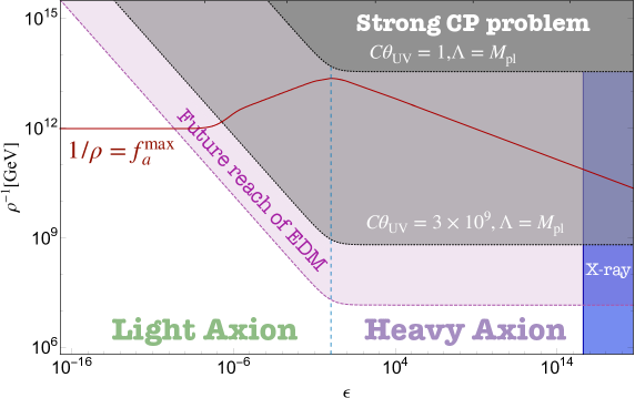
Figure 3: The parameter region of the QCD axion with aligned small instanton in $\epsilon\text{-}\rho$ plane with $\Lambda=M_{\rm pl}.$ The light gray and gray regions are excluded by the too large neutron EDM with $C\theta_{\rm UV}=3\times 10^{9}\leavevmode\nobreak\ {\rm and}\leavevmode\nobreak\ 1,$ respectively. The purple shaded range above the dashed line may be tested in future EDM searches with $C\theta_{\rm UV}=3\times 10^{9}$. On the upper frame, the maximal axion decay constant from the axion abundance is denoted (see Sec.3). The red solid line represents $1/\rho=f_{a}^{\rm max}$. The blue region is excluded by X-ray observation (by assuming dominant dark matter).

2.3 Relation to the quality problem of the PQ symmetry

The CP violation we discussed is present even when the PQ symmetry is exact (but anomalous), and thus known solutions to the quality problems may not work for the UV instantons.

The discussion is qualitatively different depending on whether $1/\rho$ is smaller or larger than the decay constant $f_{a}$. In the case of $f_{a}\ll 1/\rho$, the discussion is similar to the ordinary scenarios. In this regime, one should consider the UV contributions to the PQ breaking dynamics including the quark fields which make the PQ symmetry anomalous. For example, let us consider a model where a VEV of a scalar field $\Phi_{\rm PQ}$ breaks the PQ symmetry spontaneously. In the presence of a single pair of vector-like PQ quarks $Q_{\rm PQ}$ with an interaction

$${\cal L}\supset-y_{\Phi}\Phi_{\rm PQ}\bar{Q}_{\rm PQ}Q_{\rm PQ}$$ (11)

the potential for $\Phi_{\rm PQ}$ receives contributions from small instantons which scale as $\propto y_{\Phi}\Phi_{\rm PQ}\rho^{-3}$ or $y_{\Phi}\Phi_{\rm PQ}\rho^{-5}\Lambda^{-2}.$ The axion appears as the pseudo Nambu-Goldstone boson associated with the PQ breaking, $\langle\Phi_{\rm PQ}\rangle\sim f_{a}\ll 1/\rho$. The linear term of $\Phi_{\rm PQ}$ from the UV instanton contributes to the axion mass.

The appearance of the linear term can be avoided if $\Phi_{\rm PQ}$ is charged under some gauge symmetry like gauged $Z_{N}$ symmetry (and also we need non-trivial PQ quark contents to have color anomaly-free interaction), as in the solutions to the ordinary quality problem [27, 28, 29][30, 31, 32][59, 60, 61, 62, 63, 64, 65]. By symmetry, the small instanton contribution is suppressed as $\propto\Phi_{\rm PQ}^{N}\rho^{N-4}\leavevmode\nobreak\ {\rm or}\leavevmode\nobreak\ \Phi_{\rm PQ}^{N}\rho^{N-6}\Lambda^{-2}$, and the problem may be solved with large enough $N$. At the same time we also have the suppressed aligned contribution.

For $\left\langle{\Phi_{\rm PQ}}\right\rangle\sim f_{a}\gtrsim 1/\rho$, the problem is more serious. The reason is that the PQ field $\Phi_{\rm PQ}$ appears in the instanton through the $f_{a}$ dependence of the running gauge coupling, which means the dependence is a singular $\log{\Phi_{\rm PQ}^{N}}$ with the $Z_{N}$ gauge symmetry. This is no longer suppressed by the scales of higher dimensional terms with larger dimension for large $N$. The approach by the $Z_{N}$ symmetry does not work in this case.

In appendix A, a heavy axion model to avoid the UV problem is discussed.

Although we focused on the new CP violation in the axion models, there should be a similar CP violating effect in the case of the massless up quark solution discussed in Refs. [66, 42]. If we take into account various CP-violating higher dimensional terms, the up quark mass would receive an additional phase of $\propto(\rho\Lambda)^{-2}$. Therefore to generate the mass and preserve the vanishing strong CP phase, we need the instanton size to be large enough. One needs to check if the enough size of up-quark mass at low energy is realized in this case.

3 Axion dark matter with UV instantons

In this section, we study the cosmological abundance of the QCD axion by taking account of the small instanton.

The decay constant of the QCD axion has a window in which the axion can have a consistent cosmological history (without fine-tuning):

$$10^{8}{\rm\,GeV}\lesssim f_{a}\lesssim f_{a}^{\rm max}\simeq 10^{12}{\rm\,GeV}.$$ (12)

The lower bound comes from the duration of the neutrino burst in SN1987A [67, 68, 69, 70], the upper bound, $f_{a}^{\rm max}$, is obtained from the over production of the QCD axion in the early Universe, i.e. the axion dark matter is over abundant. The axion dark matter is realized around $f_{a}\sim f_{a}^{\rm max}$ with the initial misalignment angle $|\theta_{i}|\sim 1.$

The estimation of the abundance relies on the temperature dependence of the topological susceptibility [5, 6, 7]. (See Refs. [71, 72, 73, 74, 75] for recent lattice computations.) When the QCD axion mass becomes comparable to the Hubble parameter, the axion starts to oscillate around the potential minimum from its initial misalignment angle $\theta_{i}$. The axion number conserves and later the axion energy density behaves as dark matter. The temperature dependence of the axion mass determines when the axion starts to oscillate. The inclusion of the aligned small instanton contribution changes this temperature dependence, and the estimation of the abundance becomes non-trivial. In the following, we will estimate carefully the abundance of the axion in the presence of the small instanton.

We assume $\bar{\theta}_{\rm CP}\ll 1$ and neglect the contribution of CP violating term for a while: i.e. we use the approximation of

$$V\approx V_{\rm QCD}+V_{\rm UV}.$$ (13)

Then, the axion physical mass at the vacuum can be obtained as

$$m_{a}^{2}[\epsilon]=\frac{\chi_{0}(1+\epsilon)}{f_{a}^{2}}=m_{a}^{2}(0)(1+\epsilon).$$ (14)

The abundance formula is known for $\epsilon\gg 1$ or $\ll 1$ since we can neglect $V_{\rm QCD}$ or $V_{\rm UV}$. With only $V_{\rm UV}$ we obtain (we use the fit in Ref. [76])

$$\Omega_{a}h^{2}\approx 0.05\epsilon^{1/4}\,\bigg{(}\frac{g_{\star,\text{osc}}}{18}\bigg{)}^{-1/4}\left(\frac{\theta_{i}}{0.001}\right)^{2}\bigg{(}\frac{f_{a}}{10^{17}\,\text{GeV}}\bigg{)}^{3/2}\text{ if }\epsilon\gtrsim 1.$$ (15)

Here $g_{\star,\text{osc}}$ is the relativistic degree of freedom at the onset of oscillation.

With only $V_{\rm QCD}$ we obtain [77]

$$\Omega_{a}h^{2}\,\approx\,0.35\left(\frac{\theta_{i}}{0.001}\right)^{2}\times\begin{cases}\displaystyle\left(\frac{f_{a}}{3\times 10^{17}\,{\rm GeV}}\right)^{1.17}&f_{a}\,\lesssim\,3\times 10^{17}\,{\rm GeV\vspace{3mm}}\\ \displaystyle\left(\frac{f_{a}}{3\times 10^{17}\,{\rm GeV}}\right)^{1.54}&f_{a}\,\gtrsim\,3\times 10^{17}\,{\rm GeV}\end{cases}\text{ if }0<\epsilon\ll 1.$$ (16)

The difference of the two cases comes from the temperature dependence of the potential.

For $\epsilon\sim 1$ (more precisely $10^{-13}\text{-}10^{-6}\lesssim\epsilon\lesssim 1$ for $f_{a}=10^{8}\text{-}10^{14}{\rm\,GeV}$) , on the other hand, the abundance gets suppressed compared with $\epsilon\ll 1$ because in the presence of both terms, the time for the onset of oscillation is faster than the case of QCD potential only.

To check this we solve

$$\ddot{a}+3H\dot{a}=-\frac{\partial V}{\partial a},$$ (17)

$$\dot{s}+3Hs=0$$ (18)

with $H=\sqrt{\frac{\pi^{2}g_{\star}}{30}\frac{T^{4}}{M_{\rm pl}^{2}}}$ being the Hubble parameter in the radiation dominated Universe, $s=\frac{2\pi^{2}g_{\star s}}{45}T^{3}$ the entropy density, and $g_{\star}$ ($g_{S\star}$) the relativistic degrees of freedom (for entropy) at the cosmic temperature $T$. We evaluate the abundance parameter defined by

$$\Omega_{a}[t]\equiv\frac{\rho_{a}}{s}\frac{s_{0}}{\rho_{\rm crit}}$$ (19)

with $\rho_{a}[t]=\frac{\dot{a}^{2}}{2}+V(a),$ and $s_{0}$ and $\rho_{\rm crit}$ the current entropy density and critical density, respectively. When $T\ll T_{\rm c}$, we can easily show that this value conserves. We should also compare this with the observed dark matter abundance $\Omega_{\rm DM}h^{2}\approx 0.12$ [78].

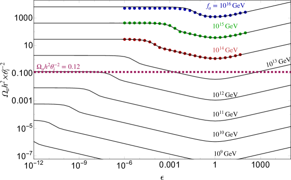
Figure 4: The resulting abundance divided by $\theta_{i}^{2}$ for the QCD axion with aligned small instanton by varying the relative instanton contribution, $\epsilon$. The data points are calculated numerically by solving the equation of motion and are for $f_{a}=10^{16,15,14}{\rm\,GeV}$ from top to bottom. The solid lines are fitted from the data and correspond to $f_{a}=10^{16,15,14,13,12,11,10,9,8}{\rm\,GeV}$ from top to bottom. The correct dark matter abundance with $\theta_{i}=1$ is denoted by the purple dotted line.

The numerical result (where we approximate the potential by the quadratic term) by varying $\epsilon$ is shown in Fig. 4 for the blue, green and red points, respectively, with $f_{a}=10^{16,15,14}{\rm\,GeV}$ from top to bottom.

For later convenience, we find a fitting formula for the abundance

$$\Omega_{a}[t\to\infty]\to\left.C_{\rm fit,1}\sqrt{\frac{\chi_{0}(1+\epsilon)}{f^{2}_{a}}}\times\frac{\sqrt{(C^{\rm fit,2}\chi(T)+\epsilon\chi_{0})/f_{a}^{2}}\theta_{i}^{2}f_{a}^{2}}{s}\frac{s_{0}}{\rho_{c}}\right|_{T=T_{\rm fit,osc}}$$ (20)

where $T_{\rm fit,osc}$ is obtained by equating $m^{\rm fit}=H$, with $m^{\rm fit}\equiv\sqrt{(C^{\rm fit,3}\chi(T)+\epsilon\chi_{0})/f_{a}^{2}}$. Here $C^{\rm fit,i}\approx\{1.03,46.2,5.35\}$ is obtained by fitting the numerical data (red points in Fig. 4) at $f_{a}=10^{14}{\rm\,GeV}.$ This formula agrees well also with the numerical results for $f_{a}=10^{15,16}{\rm\,GeV}$. We display the abundance in Fig. 4 for analytical results of smaller $f_{a}$, which requires calculation costs if we solve the equation of motion. Importantly, $10^{-13}\lesssim\epsilon\lesssim 1$, the abundance can be affected by the aligned instanton contribution, which can suppress the abundance by $\mathcal{O}(10^{-3}-1)$ for the axion with $f_{a}\gtrsim 10^{8}{\rm\,GeV}$. This suppression opens the axion window up to $f_{a}^{\rm max}[\epsilon]\lesssim 10^{13\text{-}14}{\rm\,GeV}$ with the aligned small instanton.

We overlay the maximal value of the decay constant allowed by the axion abundance as a function of $\epsilon$ in Fig. 3 (red solid line). We took $\theta_{i}=1$ in the figure. The constraints form X-ray observation are translated from Ref. [79], by assuming dominant axion dark matter (whose photon coupling is induced through the meson-axion mixing) from the misalignment mechanism in blue shaded region. The mass corresponds to $m_{a}\sim 5{\rm\,keV}$ around the boundary. The upper bound of the axion window or the natural decay constant for the axion dark matter is

$$10^{10}{\rm\,GeV}\lesssim f_{a}^{\rm max}[\epsilon]\lesssim 10^{14}{\rm\,GeV}$$ (21)

by varying $\epsilon$.

In concrete models, $\epsilon$, $\rho^{-1}$ and $f_{a}^{\rm max}$ are related. For example, in the model of Appendix A, $\rho^{-1}\sim f_{a}$. In this model, the heavy axion ($\epsilon>1$) is difficult to be the dominant dark matter from misalignment otherwise the strong CP problem exists unless $C$ has chirality suppressions. For heavy axion dark matter where we should have $f_{a}\sim 1/\rho\lesssim 10^{9}{\rm\,GeV}$ we need to consider other mechanisms to produce the correct abundance e.g. [81, 82, 83, 84, 85, 86, 87, 88, 80, 89]. This scenario needs to evade the SN1987A constraint, $f_{a}\sim 1/\rho\gtrsim 10^{8}{\rm\,GeV}$, and so the heavy axion dark matter is likely to be fully tested in the future EDM experiment.

Before ending this section, let us comment on $-1<\epsilon<0$. In this case the axion starts to oscillate towards $a/f_{a}\approx\pi$ in the early Universe and when IR contribution dominates the oscillation is around the $a\simeq 0.$ We do not consider this possibility because from phenomenological side it will cause a serious domain wall problem. If $\epsilon<-1$, it predicts $\theta_{\rm CP}=-\pi$, which is excluded from observation. In a wide class of models, we expect that the sign of the UV contributions is the same as the IR one since it is ensured by the positive path-integral measure of QCD [90].

4 Small instantons in the extra-dimension scenarios

In certain models, the integral (1) is dominated at around the UV cutoff, i.e. $\rho\sim 1/\Lambda_{\rm cutoff}.$ Once this is the case, the CP violation contribution (5) is also UV dominated, which gives

$$V_{\rm CPV}\sim-\epsilon\chi_{0}C\frac{\Lambda_{\rm cutoff}^{2}}{\Lambda^{2}}\cos\left[\frac{a}{f_{a}}+\theta_{\rm UV}\right],$$ (22)

by assuming $\Lambda_{\rm cutoff}\ll\Lambda.$

Let us first consider the case where the higher dimensional operators have no chirality suppression. In this case, $C\sim 3\times 10^{9}$ gives a large enhancement. For $\Lambda_{\rm cutoff}/\Lambda\gtrsim y_{i}$, the dominant contribution is the diagrams with multiple insertion of the higher dimensional operators. In particular with $\Lambda_{\rm cutoff}\sim\Lambda$, we obtain

$$V_{\rm CPV}\sim-\epsilon\chi_{0}C\frac{\Lambda_{\rm cutoff}^{6}}{\Lambda^{6}}\cos\left[\frac{a}{f_{a}}+\theta_{\rm UV}\right].$$ (23)

Now $C\sim 1/(y_{u}y_{d}y_{s}y_{c}y_{t}y_{b})\sim 10^{18}$ and $\theta_{\rm UV}=\mathcal{O}(1).$ To evade the EDM constraint we need

$$\epsilon C\theta_{\rm UV}\frac{\Lambda_{\rm cutoff}^{6}}{\Lambda^{6}}\lesssim 10^{-28}.$$ (24)

To be more concrete, let us study the model where the axion is originated from the gauge field in the extra dimension. The model has a nice feature to protect the PQ symmetry by the gauge invariance and the locality, and catches the essential feature of axions in string theories.

A simple realization is possible in five dimensional model with the fifth dimension compactified by an orbifold $S_{1}/Z_{2}$ [91]. The gluon lives in the fifth dimensional bulk with size $R$ and the axion is identified as the Wilson line of the fifth direction of a $\mathop{\rm U}(1)$ gauge field. The cut-off scale of the theory is identified as the 5d planck scale,

$$\Lambda_{\rm cutoff}\sim(M_{\rm pl}^{2}/R)^{1/3},$$ (25)

if there is no other interactions which gets strong below this scale. We consider the case where the quarks and the Higgs field live on the orbifold fixed point. The PQ symmetry is identified as the shift symmetry of the $A_{5}$ component of the $\mathop{\rm U}(1)_{\rm PQ}$ gauge field on the boundary. While it is protected by the gauge symmetry and locality, the mixed Chern-Simons term,

$${k\over 8\pi^{2}}\int A_{\rm U(1)_{\rm PQ}}F_{\rm SU(3)_{c}}F_{\rm SU(3)_{c}},$$ (26)

can give the anomalous coupling between the axion and the gluons. This setup provides a very simple origin of the axion (i.e. string axion). In this model, the axion has a decay constant

$$f_{a}\sim 1/R.$$ (27)

On the brane, we have “Planck scale” suppressed terms similar to (3) i.e.

$$\Lambda\sim\Lambda_{\rm cutoff}.$$ (28)

The aligned contributions is studied in Ref. [44], where the 5d instanton solution is found to contribute as

$$\chi_{\rm aligned}[R]=\epsilon[R]\chi_{0}=\Pi_{i}\left(\frac{y_{i}}{4\pi}\right)\int_{1/\Lambda_{\rm cutoff}}^{R}{\frac{d\rho^{\prime}}{\rho^{\prime 5}}e^{-S_{\rm eff}[1/\rho^{\prime}]}F^{(\rm 5D)}[\rho^{\prime}]}.$$ (29)

where

$$F^{(\rm 5D)}[\rho^{\prime}]=1.5\times 10^{-3}\left(\frac{2\pi}{\alpha_{s}(1/R)}\right)^{6},S_{\rm eff}=\left(\frac{2\pi}{\alpha^{\rm SM}_{s}(1/R)}-3\xi(R/\rho^{\prime})\frac{R}{\rho^{\prime}}+b_{0}\log\left(\frac{R}{\rho^{\prime}}\right)\right).$$ (30)

The function, $\xi$, which increases to approach to $\sim 0.35$ with $R/\rho^{\prime}\to R\Lambda_{\rm cutoff}$, can be found in [44]. The beta function coefficient, $b_{0}$, and the coupling constant, $\alpha_{s}^{\rm SM},$ are, respectively, given by

$$b_{0}=7\leavevmode\nobreak\ {\rm and}\leavevmode\nobreak\ 1/\alpha^{\rm SM}_{s}(1/R)\equiv 1/\alpha_{s,{\rm EW}}-b_{0}/(2\pi)\log{(v_{\rm EW}R)}$$ (31)

with $\alpha_{s,{\rm EW}}=0.118$ and $v_{\rm EW}=100{\rm\,GeV}.$ The suppression of $S_{\rm eff}$ at large $1/\rho^{\prime}$ makes the integral dominated around $\rho^{\prime}\sim 1/\Lambda_{\rm cutoff}.$ Here, the fundamental 5d gauge coupling, $g_{5}^{2}$, (dimension -1) is matched to the SM gauge coupling as

$$g_{5}^{2}=4\pi^{2}R\times\alpha^{\rm SM}(1/R).$$ (32)

Since the gauge interaction is from a higher dimensional term, the theory gets strong at a scale $\sim 24\pi^{3}/g_{5}^{2}$.

Considering a diagram as in Fig. 2, we obtain

$$\chi_{\rm CPV}[R]\sim\left(\frac{1}{\Lambda^{2}}\right)(y_{u}y_{d})^{-1}\left(\Pi_{i}\frac{y_{i}}{4\pi}\right)\int_{1/\Lambda_{\rm cutoff}}^{R}{\frac{d\rho^{\prime}}{\rho^{\prime 5}}\rho^{\prime-2}e^{-S_{\rm eff}[1/\rho^{\prime}]}F^{(\rm 5D)}[\rho^{\prime}]}.$$ (33)

By numerically performing this integral, we confirm the previous general argument at a good precision with $C\sim 10^{9}$ by taking the ratio of Eq. (33) to Eq. (29) with $\Lambda\sim\Lambda_{\rm cutoff}.$ In this model, however, the dominant contribution is from the term corresponding to (23).

$$\chi_{\rm CPV}[R]\sim\left(\frac{1}{16\pi^{2}\Lambda^{2}}\right)^{3}\int_{1/\Lambda_{\rm cutoff}}^{R}{\frac{d\rho^{\prime}}{\rho^{\prime 5}}\rho^{\prime-6}e^{-S_{\rm eff}[1/\rho^{\prime}]}F^{(\rm 5D)}[\rho^{\prime}]}.$$ (34)

This is again consistent with our general argument.

In the case of $\Lambda\sim\Lambda_{\rm cutoff}$, however, it is natural to assume that there are chirality suppressions for the higher dimensional terms, so that the small coupling constants, such as $y_{u}$ and $y_{d}$, are stable under the radiative corrections. Then (3) is in the form,

$$C_{ud}^{ijkl}=C_{ud}Y_{u}^{ij}Y_{d}^{kl},$$ (35)

with

$$C_{ud}\sim\mathcal{O}(1)+i\mathcal{O}(1).$$ (36)

Then we obtain

$$\chi^{\rm CS}_{\rm CPV}[R]=\left(\frac{1}{\Lambda_{\rm eff}^{2}}\right)\left(\Pi_{i}\frac{y_{i}}{4\pi}\right)\int_{1/\Lambda_{\rm cutoff}}^{R}{\frac{d\rho^{\prime}}{\rho^{\prime 5}}\rho^{\prime-2}e^{-S_{\rm eff}[1/\rho^{\prime}]}F^{(\rm 5D)}[\rho^{\prime}]}.$$ (37)

Here we introduced $\Lambda_{\rm eff}$ for a later convenience. This satisfies $\Lambda_{\rm eff}\sim\Lambda\gtrsim\Lambda_{\rm cutoff}$ and it includes $|C_{ud}|$ as well as relative numerical uncertainty compared with the integral in Eq. (29). This contribution may be suppressed compared with the aligned instanton constribution by $\left(\Lambda_{\rm cutoff}/\Lambda_{\rm eff}\right)^{2}.$

The resulting parameter region by calculating $\chi_{\rm CPV}/(\chi_{0}+\chi_{\rm aligned})$ is shown in Fig. 5 by the red solid line. The red dashed line in Fig. 5 is for the chirality-suppressed case by assuming $\Lambda_{\rm eff}=\Lambda=\Lambda_{\rm cutoff}.$ The gray (purple) region is the bound (future reach) from nucleon EDM experiments by assuming $\theta_{\rm UV}\sim 1$. Interestingly with $1/R\gtrsim 10^{15-16}{\rm\,GeV}$ we have an allowed region. This is because in this setup $g_{5}^{2}\Lambda_{\rm cutoff}\propto(M_{\rm pl}^{2}R^{2})^{1/3}\alpha^{\rm SM}_{s}(1/R)$ which makes the gauge interaction at around the cut-off weaker for smaller $R$. In this regime, the axion mass is dominated by the IR QCD contributions, and the low-energy axion physics is the same as the conventional one.

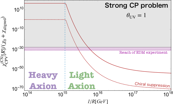
Figure 5: Allowed regions for the extra-dimension model by numerically integrating the small instanton contributions (29), (33) and (37), with $\Lambda^{3}R=M_{\rm pl}^{2}$ and $\Lambda=\Lambda_{\rm cutoff}$. The red solid (dashed) line represents $\chi_{\rm CPV}/(\chi_{0}+\chi_{\rm aligned})$ ($\chi_{\rm CPV}^{\rm CS}/(\chi_{0}+\chi_{\rm aligned})$). The EDM bound (gray region) and the future reach (purple region) is estimated by assuming $\theta_{\rm UV}\sim 1.$

5 Cosmology of extra-dimensional axions

The scenario of the axion from extra-dimension is a natural possibility for the solution of the strong CP problem. We have seen in the previous section that the radius of the extra dimension is required to be above the scale of the grand unification theory (GUT), $10^{15}\leavevmode\nobreak\ {\rm GeV}$, in order to avoid yet another strong CP problem from the UV instantons. The axion decay constant $f_{a}$ is also required to be above the GUT scale. In other words, we need the gauge coupling to be weakly coupled up to the 5d Planck scale also for solving the strong CP problem. This sounds quite natural in string theories or in general in the theory of quantum gravity, where the typical scale is the GUT or the Planck scale. However, cosmologically, it implies that the axion has an overproduction problem if we do not require a fine-tuning of the initial misalignment angle $\theta_{i}.$

In the extra-dimensional scenario, we find that there is a simple possibility to avoid the overproduction and realize the axion dark matter naturally by the help of the UV instantons. We mainly consider the case where the higher dimensional operators have chirality suppressions. The case with no chirality suppression will also be discussed later.

5.1 Natural axion dark matter

In the extra dimensional scenario, there is a modulus field, the radion, to represent the size of the extra dimension. In the current Universe, the radion field $r$ is stabilized at $\left\langle{r}\right\rangle=R$. By saying that the radion is a dynamical field, we implicitly assume that the mass, $m_{r}^{2}\equiv V^{\prime\prime}[r]$, is not extremely heavy. We will come back to the dynamics of the radion in Sec. 5.2

Then, it is possible during the inflation that $r$ is displaced from the current location. This changes the coupling of 4d gravity via

$${\cal L}\sim\Lambda^{3}r{\cal R}.$$ (38)

In the following we perform a Weyl transformation to move to the Einstein frame, so that the coefficient of the Ricci scalar is always $M_{\rm pl}^{2}.$ Instead, various potentials at the zero temperature obtain an additional factor of ${M_{\rm pl}^{4}}/{(\Lambda^{3}r)^{2}}.$ For instance the axion potential from QCD is

$$\tilde{V}_{\rm QCD}[r,a]=\tilde{\chi}_{\rm QCD}[r]\left(1-\cos{\frac{a}{f_{a}}}\right).$$ (39)

Here we use

$$\tilde{\chi}_{\rm QCD}[r]\sim\frac{M_{\rm pl}^{4}}{(\Lambda^{3}r)^{2}}(\Pi_{i}y_{i})\Lambda_{\rm QCD}[r]^{4}$$ (40)

with

$$\Lambda_{\rm QCD}[r]\approx\exp{\left(-\frac{2\pi}{b_{0}\alpha_{s}(1/r)}+\frac{2\pi}{b_{0}\alpha^{\rm SM}_{s}(1/R)}\right)}\Lambda_{\rm QCD}[R]$$ (41)

and $\Lambda_{\rm QCD}[R]\sim 400{\rm\,MeV}.$ We emphasize that

$$\alpha_{s}[1/r]=\frac{g_{5}^{2}}{4\pi^{2}r}$$ (42)

and $g_{5}^{2}$ is fixed by (32) once $\left\langle{r}\right\rangle=R$ is given. This form is a good approximation when the QCD scale, $\Lambda_{\rm QCD}[r]$, is higher than the electroweak scale. The chirality flips are supplied by the Yukawa interactions whereas the VEV of the Higgs field is induced by the chiral symmetry breaking of ${\rm SU{(}}6)\times{\rm SU{(}}6)\to{\rm SU{(}}6)$. Due to the top quark condensation, the Higgs field obtains an expectation value $\left\langle{H}\right\rangle_{r}\sim\Lambda_{\rm QCD}[r],$ with $\left\langle{}\right\rangle_{r}$ denotes the expectation value in a spatially homogeneous radion background $r$. More precisely, there could be CP-violating effect to the IR QCD contribution via not only the higher dimensional operators but also from the SM interactions through the CKM phase e.g. [56]. The latter contribution is estimated to be at most comparable to the QCD potential in Eq. (39). Although this could be important in some cases, we are particularly interested in the case that $\tilde{V}_{\rm QCD}$ is not the dominant contribution and thus the effects can be ignored in the most successful parameter region. One should keep in mind that there can be significant corrections from weak interactions when $\tilde{V}_{\rm QCD}$ is important.

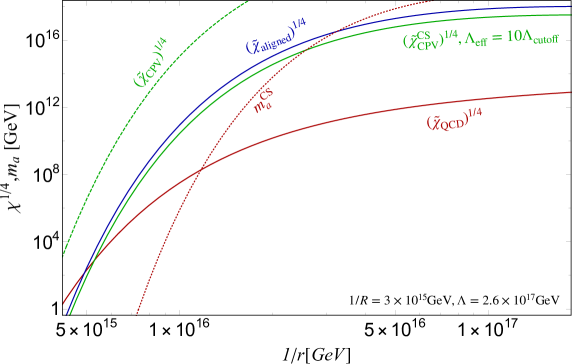
Figure 6: Various contributions and axion mass (with chiral suppressions) with a dynamical radion field, $r$. We fix $1/R=3\times 10^{15}{\rm\,GeV},\Lambda=\Lambda_{\rm cutoff}=1/10\Lambda_{\rm eff}\leavevmode\nobreak\ {\rm and}\leavevmode\nobreak\ \Lambda^{3}R=M_{\rm pl}^{2}.$

On the contrary the CP violating small instanton contribution is estimated as

$$\tilde{V}_{\rm CPV}[r,a]\approx-\tilde{\chi}^{\rm(CS)}_{\rm CPV}[r]\cos{[\frac{a}{f_{a}}+\theta_{\rm UV}]}.$$ (43)

Here,

$$\tilde{\chi}^{\rm(CS)}_{\rm CPV}[r]=\frac{M_{\rm pl}^{4}}{(\Lambda^{3}r)^{2}}\chi^{\rm(CS)}_{\rm CPV}[r].$$ (44)

Similarly we get the aligned contribution,

$$\tilde{\chi}_{\rm aligned}[r]=\frac{M_{\rm pl}^{4}}{(\Lambda^{3}r)^{2}}\chi_{\rm aligned}[r].$$ (45)

$\tilde{\chi}^{\rm(CS)}_{\rm CPV}[r],\tilde{\chi}_{\rm QCD}[r]\leavevmode\nobreak\ {\rm and}\leavevmode\nobreak\ \tilde{\chi}_{\rm aligned}[r]$ as well as $m_{a}^{\rm CS}[r]\equiv r\sqrt{\tilde{\chi}_{\rm QCD}[r]+\tilde{\chi}_{\rm aligned}[r]}$ are evaluated numerically and are shown in Fig. 6. We fix $1/R=3\times 10^{15}{\rm\,GeV}$. First, we can see that the all contributions increase with increasing $1/r$. This is because the coupling $\alpha_{s}[1/r]\propto 1/r$ increases. Thus the exponential suppressions in all instanton contributions are alleviated (see Refs. [92, 93, 91, 94, 83, 95] for stronger QCD, Ref. [96] for stronger small instanton by enhancing Yukawa couplings.). Second, the CPV contribution as well as the aligned contribution increases faster than the IR QCD contribution does. This is because the exponential suppression in $\chi_{\rm aligned}\leavevmode\nobreak\ {\rm or}\leavevmode\nobreak\ \chi^{\rm(CS)}_{\rm CPV}$, $\propto e^{-\frac{2\pi}{\alpha_{s}[1/r]}}$ is larger than that of $\chi_{\rm QCD}$, $\propto e^{-\frac{4}{7}\times\frac{2\pi}{\alpha_{s}[1/r]}}.$ (Here we neglect the second and third terms in (30) for analytic argument since they are irrelevant in the weakly coupled region to satisfy the EDM bound.) At larger $1/r$, the former increases faster.

This feature is important in our mechanism: if $r=r_{\rm inf}$ during inflation is smaller than $R$, one may obtain the UV instanton contribution dominating over the IR contribution. Furthermore, the axion mass can easily satisfy

$$m_{a}[r_{\rm inf}]\gtrsim H_{\rm inf}$$ (46)

with $H_{\rm inf}$ being the Hubble parameter during inflation. We find that the axion, then, is stabilized at a CP-violating position,

$$\theta_{r_{\rm inf}}\sim\theta_{\rm UV}\min[\chi_{\rm CPV}^{(\rm CS)}[r_{\rm inf}]/\chi_{\rm aligned}[r_{\rm inf}],1].$$ (47)

After the inflation the radion either rapidly or slowly settle into the minimum of the potential [97, 98]. In any case, since the IR QCD contribution is absent due to the finite temperature effect from inflaton decays (by assuming the SM radiation temperature is higher than the QCD scale), $\theta_{r_{\rm inf}}$ is kept intact after inflation until the temperature decreases to around the QCD scale. This means

$$\theta_{i}=\theta_{r_{\rm inf}}.$$ (48)

If the chiral suppression were absent in the higher dimensional operators, this mechanism would give the initial misalignment of order $\theta_{\rm UV}\sim 1$, and the axion would be overproduced.

On the other hand, with chirality suppressions, we find

$$\theta_{i}\sim\theta_{\rm UV}\frac{\tilde{\chi}^{\rm CS}_{\rm CPV}}{\tilde{\chi}_{\rm aligned}}\sim\theta_{\rm UV}\left(\frac{\Lambda_{\rm cutoff}}{\Lambda_{\rm eff}}\right)^{2}\sim 1\leavevmode\nobreak\ \%\times\theta_{\rm UV}\left(\frac{\Lambda_{\rm cutoff}/\Lambda_{\rm eff}}{0.1}\right)^{2}.$$ (49)

Consequently the axion dark matter can be explained by using Eq. (16) in a wide range of parameters satisfying $H_{\rm inf}\lesssim m_{a}[r_{\rm inf}]$ and UV instanton dominance. Although we need a mild tuning on $\Lambda_{\rm cutoff}/\Lambda_{\rm eff}$, $\Lambda_{\rm cutoff}/\Lambda_{\rm eff}<1$ may be needed for a weakly coupled theory.

The allowed region in Fig. 6 is consistent with the upper bound of

$$H_{\rm inf}\lesssim 6\times 10^{13}{\rm\,GeV}$$ (50)

from the constraint for the tensor-to-scalar ratio [99] for $1/r_{\rm inf}\gtrsim 10^{16}{\rm\,GeV}$. On the other hand, in the region $1/r_{\rm inf}\gg 10^{17}{\rm\,GeV}$, should be avoided since the potential energy from QCD exceeds that during the inflation.

5.2 Dynamics of $r$ and parameter regions

Let us consider the radion mass during inflation. We may take the radion nearly massless in 5d by assuming that the brane position is not strongly fixed. Since the radion kinetic term in the Einstein frame is given by (e.g. [100])

$${\cal L}=\frac{3}{4}M_{\rm pl}^{2}(\partial\log{r})^{2},$$ (51)

it couples to other fields through Planck suppressed operator with normalized kinetic terms. In any case there is a radiative induced mass after the compactification. This mass may be dominated by the bulk gauge/gravity interaction [100] $\sim{1/(16\pi^{2}R^{4}M_{\rm pl}^{2})}$, which sets the lower bound of the radion mass without a tuning:

$$m_{r}[R]\gtrsim 10^{10}{\rm\,GeV}\left(\frac{10^{15}{\rm\,GeV}}{1/R}\right)^{2}.$$ (52)

In addition the brane localized potential may give heavier mass to the radion. In the following we take $m_{r}^{2}$ arbitrary to check which mass range of the radion is consistent with the previous discussion. While we implicitly assume that the inflaton field to drive inflation is not the radion itself, it is possible to identify those two fields as we briefly mention in Sec.5.3.

During the inflation, the radion field value may be different from $R$. In general the radion would acquire a run-away potential $V_{\rm runaway}\sim\left(\frac{M_{\rm pl}^{2}}{r\Lambda^{3}}\right)^{2}H_{\rm inf}^{2}M_{\rm pl}^{2}$. This biases $r$ to a larger value. The localized radion potential on the brane may involve both inflaton and radion. This can give an interaction between the radion and inflaton. We note that there is also a contribution from the QCD instanton to the radion mass squared $\delta m_{r}^{2}[r]\sim\frac{\sqrt{\tilde{\chi}_{\rm aligned}+\tilde{\chi}_{\rm QCD}}}{M_{\rm pl}}$ which is always subdominant to the Hubble induced mass if the QCD potential is negligible compared to inflation energy density.

To be generic we consider the radion-inflaton potential in the form of

$$V=m_{r}^{2}[R]\frac{A^{2}}{2}+{C_{\rm inf}H_{\rm inf}^{2}M_{\rm pl}}A$$ (53)

where $A\equiv\sqrt{\frac{3}{2}}M_{\rm pl}\log{(r/R)}$ is the radion with the kinetic normalization. $C_{\rm inf}$ denotes the interaction strength between inflaton and $r$ in the 4D Planck unit. This should be a good description when $r_{\rm inf}$ is not too much deviated from $R$. Then we obtain

$$\frac{1}{r_{\rm inf}}=\frac{1}{R}\exp{\left(\frac{C_{\rm inf}H^{2}_{\rm inf}}{m_{r}^{2}[R]}\right)}.$$ (54)

This gives $r_{\rm inf}\ll R$ if $C_{\rm inf}>0$ and

$$H_{\rm inf}\gtrsim{C^{-1/2}_{\rm inf}}m_{r}[R].$$ (55)

By concerning Eq. (52), the inflation scale turns out to be in the range

$$H_{\rm inf}\gtrsim C_{\rm inf}^{-1/2}10^{10}{\rm\,GeV}\left(\frac{10^{15}{\rm\,GeV}}{1/R}\right)^{2}.$$ (56)

This is consistent with Eq. (50).

For $r_{\rm inf}$ much larger or smaller than $R$, the expansion in (53) is invalid. One should instead define $A$ with $R$ replaced by $r_{\rm inf}$ to conduct a similar discussion. The same lower bound on $H_{\rm inf}$ is obtained where $1/R$ is replaced by $1/r_{\rm inf}$.

Notice that we can only have $1/R\gtrsim 10^{15}{\rm\,GeV}$ to avoid the strong CP problem. From Fig.6, we find that with $1/r_{\rm inf}\sim[1.5-3]\times 10^{16}{\rm\,GeV}$ we can have (46). For larger $1/r_{\rm inf}$, the UV instanton contribution is larger than the upper bound of the inflation scale (50). Consequently we find that our mechanism works for high scale inflation.

To explain the parameter region, we display $\theta_{i}\times\left(\frac{\Lambda_{\rm cutoff}}{\Lambda_{\rm eff}}\right)^{-2}$ in the upper panel of Fig. 7 for $1/R=5\times 10^{15}{\rm\,GeV},10^{16}{\rm\,GeV}\leavevmode\nobreak\ {\rm and}\leavevmode\nobreak\ 2\times 10^{16}{\rm\,GeV}$ from left to right. Here we take $\theta_{i}=\left\langle{a/f_{a}}\right\rangle_{r}=\tilde{\chi}^{\rm CS}_{\rm CPV}/(\tilde{\chi}_{\rm aligned}+\tilde{\chi}_{\rm QCD})$. Those values are calculated by using Eqs. (29) and (37) with multiplying $M_{\rm pl}^{4}/(r\Lambda_{\rm cutoff}^{3})^{2}$ and Eq. (40). We also colored the range above $1\%$ which may account for the axion dark matter with $\Lambda_{\rm cutoff}/\Lambda_{\rm eff}\gtrsim\mathcal{O}(10)\%.$ Larger than a critical point, $\theta_{i}$ approaches to a constant irrelevant to $r_{\rm inf}$ and $1/R$ when $1/R\lesssim 10^{16}{\rm\,GeV}$. This $r_{\rm inf}$ insensitive region is what we have been focusing on. Smaller than the critical point we also have a tiny parameter region. In the lower panel we present the corresponding $\tilde{\chi}_{\rm aligned}\leavevmode\nobreak\ {\rm and}\leavevmode\nobreak\ \tilde{\chi}_{\rm QCD}$ by red solid and dashed lines respectively. We can see that $m_{a}^{\rm CS}[r_{\rm inf}]$ can be larger than $\sim 10^{10}{\rm\,GeV}$, and satisfy both (46) and (56) with $1/R\lesssim 10^{16}{\rm\,GeV}$. As a result, the parameter region for this scenario is

$$1/R\sim 10^{15}{\rm\,GeV}\text{-}10^{16}{\rm\,GeV}\leavevmode\nobreak\ {\rm and}\leavevmode\nobreak\ H_{\rm inf}\sim C_{\rm inf}^{-1/2}10^{10}{\rm\,GeV}\text{-}10^{14}{\rm\,GeV}.$$ (57)

This region may be searched for in the future EDM experiments and the measurement of the tensor-to-scalar ratio. If the scale is linked to the proton decay operator we may further have implications in the experiments searching for the proton decay (see the next section).

When $1/R\gg 2\times 10^{16}{\rm\,GeV}$, on the other hand, $\theta_{i}$ and $m^{\rm CS}_{a}[r_{\rm inf}]$ are too small for our mechanism to work. However we may have other mechanism to explain the axion dark matter. It was shown that if inflation lasts long, $\theta_{i}$ approaches to the Bunch-Davies distribution [101, 102]. In particular, when $(\tilde{\chi}_{\rm QCD}+\tilde{\chi}_{\rm aligned})^{1/4}\sim H_{\rm inf}$ we may again obtain dominant axion dark matter. However, since $m^{\rm CS}_{a}[r_{\rm inf}]\ll H_{\rm inf}$, the axion is almost massless during inflation. There is a constraint on the axion quantum fluctuation from the isocurvature of density perturbation [99], which sets an upper bound on the inflation scale:

$$H_{\rm inf}\lesssim 10^{9}{\rm\,GeV}\left(\frac{f_{a}}{10^{16}{\rm\,GeV}}\right)^{0.408}.$$ (58)

This can be satisfied with $C_{\rm inf}\gtrsim 100$. We have checked that when $1/R\lesssim 10^{17}{\rm\,GeV}$ there exists $r_{\rm inf}$ to satisfy $(\tilde{\chi}_{\rm QCD}+\tilde{\chi}_{\rm aligned})^{1/4}\sim H_{\rm inf}\sim 10^{9}{\rm\,GeV}.$ If $C_{\rm inf}$ is not extremely large, the scenario may be tested in the future CMB observation of the isocurvature perturbation.

Lastly, let us comment the case without chirality suppressions. In this case, we can still obtain the axion dark matter similar to the discussion here. However the inflation scale is extremely low with $H_{\rm inf}\ll 1{\rm\,GeV}$ (see Fig.6) and the radion mass needs to be very light, which may require certain tuning.

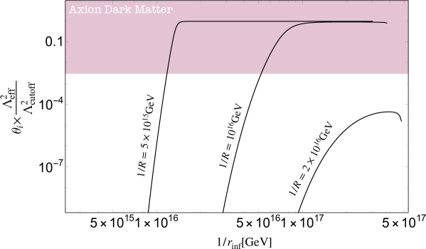
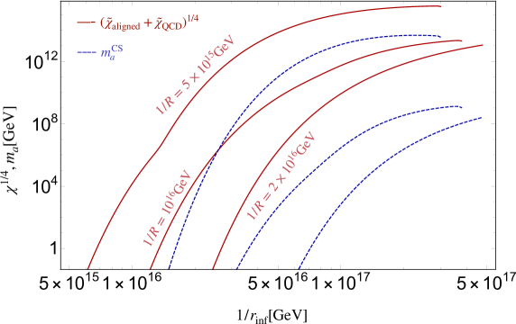
Figure 7: The resulting misalignment angle of chiral suppression scenario if axion field is set at the potential minimum at $r=r_{\rm inf}$ during inflation [upper panel]. The region can explain the dominant axion dark matter with $\Lambda_{\rm cutoff}/\Lambda_{\rm eff}\lesssim 1$ is shown in purple. The corresponding topological susceptibility^1/4 [red solid line] and axion mass [blue dashed line] neglecting CPV contribution with general $r$ are also shown [lower panel].

5.3 More unified pictures

More minimally, radion may be the inflaton. In this case it must be away from the potential minimum, $r=R$, during inflation. We need to make the radion potential flat enough at around $r\sim 1/\Lambda_{\rm cutoff}$ to drive a hilltop inflation. This is always possible if we can write down a general localized potential on a brane. In this case, if we can take the potential arbitrary flat, in principle we can have arbitrary small $H_{\rm inf}$.

An interesting question is whether we can build a GUT model broken at a scale of $1/R$. Let us consider a simple GUT gauge group in the bulk and matters are localized on a brane. We expect not too different size of small instanton contribution from that discussed in the main part since the exponential term has the exponent $S_{\rm eff}\sim 2\pi/\alpha_{s}\approx 2\pi/\alpha_{\rm GUT}\approx 8\pi^{3}R/g_{5}^{2}$ in the weakly coupled limit, with $\alpha_{\rm GUT}$ being the GUT gauge coupling constant. Therefore, if the small instanton (from GUT) is still aligned to the IR contribution, we expect the similar scenario. An interesting prediction then is the proton decay. The relevant higher dimensional operators, are suppressed by $R^{2}$. Therefore the decay constant of the axion is linked to the proton decay rate. However, the breaking of GUT may induce a small instanton with CPV to the axion potential even in the renormalizable theory (c.f. [47]). Whether the axion dark matter scenario works would depend on the detail of the GUT models.

6 Conclusions

The axion window, $10^{8}\leavevmode\nobreak\ {\rm GeV}\lesssim f_{a}\lesssim 10^{12}\leavevmode\nobreak\ {\rm GeV}$, has been discussed as the allowed region for the QCD axion models. The upper bound, $10^{12}$ GeV, is put by cosmological considerations where the misalignment of the axion value in the early Universe produces the axion energy density at later time as oscillations about the true minimum of the potential. This upper bound has given a theoretical challenge to lower the decay constant much below the scale of grand unification or quantum gravity.

The challenge should however be considered carefully. In the UV physics, there can be unknown significant contribution to the axion mass which may be aligned to the low energy QCD contributions so that the strong CP problem is still solved. Also, the UV physics may modify the axion potential in the early Universe so that the upper bound itself is not reliable.

We discussed that the UV contribution, if it is dominated by high scale physics such as the Planck scale, is severely constrained by a new CP violation caused by the combination of instantons and higher dimensional operators. Especially, in the model where the axion arises from a gauge field in the extra dimension, such as string axions, the new CP problem excludes the possibility for the UV contributions to overwhelm the ordinary low energy QCD contributions. The consistent scenario is only possible for the size of the extra dimension, i.e., the axion decay constant, to be larger than about $10^{15-16}$ GeV which is beyond the axion window.

It is however important to realize that the UV contribution can be much larger during the cosmological inflation as the size of the extra dimension can be different from the current one. By considering the enhancement of the QCD coupling during the inflation, the minimum of the axion potential is located near the current minimum in a wide range of parameters, so that a small misalignment angle is realized. Even for a large decay constant, such as $f_{a}\sim 10^{15-16}\leavevmode\nobreak\ {\rm GeV}$, axion abundance can naturally be that of dark matter of the Universe while the strong CP problem is still solved. This discussion opens up the possibility of natural string or GUT axion scenarios where inflation dynamics is tied to the size of the compactified directions. The upper bound on the axion window should not be taken so seriously in string models.

Appendix A A model of heavy axion from accidental PQ symmetry

To have a closer look of the quality problem raised here. Let us build a new kind of heavy axion model, and discuss the CP violation. Let us consider again $Z_{N}$ (gauge) symmetry to solve the ordinary quality problem and “define” the PQ symmetry. We consider $N$ fundamental quark pairs, $\bar{Q}_{\rm PQ}^{a},{Q}_{\rm PQ}^{a}$ with interaction of

$${\cal L}\supset-\Phi_{\rm PQ}\sum_{a}y_{\Phi}^{(a)}\bar{Q}^{a}_{\rm PQ}Q^{a}_{\rm PQ}.$$ (59)

Under $Z_{N}$, $\Phi_{\rm PQ}^{*},\leavevmode\nobreak\ {\rm and}\leavevmode\nobreak\ \bar{Q}_{\rm PQ}^{a}$ transform with a phase of $-2\pi/N$, $Q_{\rm PQ}$ is a singlet. The quark masses are assumed to be around the PQ scale $f_{a}$, i.e. $y^{(a)}_{\Phi}\sim 1.$ In addition, we introduce $N_{\phi}$ of fundamental colored scalars, $\phi_{i}$, around the mass scale, $m_{\phi}$. Then Eq. (1) can be denoted as the integral by parts as

$${\cal L}^{\rm(vac)}_{\rm eff} \sim\int^{1/m_{\phi}}_{1/f_{a}}{\frac{d\rho^{\prime}}{\rho^{\prime 5}}e^{-S^{(1)}_{\rm eff}[1/\rho^{\prime}]}\ F^{\rm(1)}[\rho^{\prime}]\det{\frac{Y_{u}}{4\pi}}\det{\frac{Y_{d}}{4\pi}}}\cos{\left(\frac{Na}{f_{a}}\right)}$$ (60)

$$+\int^{1/f_{a}}_{1/\Lambda_{\rm cutoff}}{\frac{d\rho^{\prime}}{\rho^{\prime 5}}\rho^{\prime N}f_{a}^{N}e^{-S^{(2)}_{\rm eff}[1/\rho^{\prime}]}\ F^{\rm(2)}[\rho^{\prime}]\det{\frac{Y_{u}}{4\pi}}\det{\frac{Y_{d}}{4\pi}}}\cos{\left(\frac{Na}{f_{a}}\right)}.$$ (61)

If the number of $\phi$, $N_{\phi}$ is large enough, the gauge coupling is no longer asymptotically free. Then we can obtain

$$\exp{[-S^{(1,2)}_{\rm eff}]}\propto\rho^{\prime b_{1,2}}$$ (62)

with $b_{1}=b_{0}-N_{\phi}/6$ and $b_{2}=b_{0}-N_{\phi}/6-2N/3$. Neglecting the $\rho^{\prime}$ dependence in $F^{(i)}[\rho^{\prime}],$ the integral may dominates around

$$\rho_{\rm case1}\sim 1/m_{\phi},\rho_{\rm case2}\sim 1/f_{a},\rho_{\rm case3}\sim 1/\Lambda_{\rm cutoff},$$ (63)

depending on $N_{\phi}\leavevmode\nobreak\ {\rm and}\leavevmode\nobreak\ N.$ The first case is not at all problematic because $S_{\rm eff}[1/\rho]\approx 2\pi/\alpha_{\rm SM}[1/\rho],$ which is around the suppressed SM contribution. The third case may induce an additional potential to axion but it can be suppressed by assuming a large $N$ as the ordinary solution to the quality problem, i.e. in this case the term is suppressed by $f_{a}^{N}/\Lambda_{\rm cutoff}^{N-4}$. This also says that with increasing $N$ the case 3 approaches to the case 2 since the integral in (61) tends to dominate at IR.

The case 2, the integral dominates at $\rho\sim 1/f_{a},$ may generate additional axion mass. Then we get the small instanton contribution as

$$\epsilon\chi_{0}\sim 10^{-23}f_{a}^{4}\times\left(\frac{2\pi}{\alpha_{s}[f_{a}]}\right)^{6}e^{-\frac{2\pi}{\alpha_{s}[f_{a}]}}.$$ (64)

with

$$e^{-\frac{2\pi}{\alpha_{s}[f_{a}]}}\sim\left(\frac{0.05{\rm\,GeV}}{m_{\phi}}\right)^{b_{0}}\left(\frac{m_{\phi}}{f_{a}}\right)^{b_{1}}.$$ (65)

If $-b_{1}+4\geq 0$, this contribution is enhanced. For instance with $N_{\phi}=60$  and $f_{a}=8\times 10^{8}$, we get $\epsilon\sim 10^{5}$ and obtain the heavy axion. Here $\alpha_{s}[f_{a}]\sim 0.12.$ We do not need to care the UV contribution since we can take $N$ large enough to suppress it. But we should make sure that before the coupling blows up, there is some UV completion appear (by integrating out which we may have another small instanton effect but again it is suppressed as long as $N$ is large). Then (8) suggests $1/\rho\sim f_{a}\lesssim 10^{10}{\rm\,GeV}$ when $\epsilon\gg 1.$ The parameter region of the axion dark matter of this model is shown by the red line in Fig. 3.

References

- [1] R. D. Peccei and H. R. Quinn, Phys. Rev. Lett. 38, 1440-1443 (1977) doi:10.1103/PhysRevLett.38.1440
- [2] R. D. Peccei and H. R. Quinn, Phys. Rev. D 16, 1791-1797 (1977) doi:10.1103/PhysRevD.16.1791
- [3] S. Weinberg, Phys. Rev. Lett. 40, 223-226 (1978) doi:10.1103/PhysRevLett.40.223
- [4] F. Wilczek, Phys. Rev. Lett. 40, 279-282 (1978) doi:10.1103/PhysRevLett.40.279
- [5] L. F. Abbott and P. Sikivie, Phys. Lett. B 120, 133-136 (1983) doi:10.1016/0370-2693(83)90638-X
- [6] J. Preskill, M. B. Wise and F. Wilczek, Phys. Lett. B 120, 127-132 (1983) doi:10.1016/0370-2693(83)90637-8
- [7] M. Dine and W. Fischler, Phys. Lett. B 120, 137-141 (1983) doi:10.1016/0370-2693(83)90639-1
- [8] E. Witten, Phys. Lett. B 149, 351-356 (1984) doi:10.1016/0370-2693(84)90422-2
- [9] P. Svrcek and E. Witten, JHEP 06, 051 (2006) doi:10.1088/1126-6708/2006/06/051 [arXiv:hep-th/0605206 [hep-th]].
- [10] J. P. Conlon, JHEP 05, 078 (2006) doi:10.1088/1126-6708/2006/05/078 [arXiv:hep-th/0602233 [hep-th]].
- [11] A. Arvanitaki, S. Dimopoulos, S. Dubovsky, N. Kaloper and J. March-Russell, Phys. Rev. D 81, 123530 (2010) doi:10.1103/PhysRevD.81.123530 [arXiv:0905.4720 [hep-th]].
- [12] B. S. Acharya, K. Bobkov and P. Kumar, JHEP 11, 105 (2010) doi:10.1007/JHEP11(2010)105 [arXiv:1004.5138 [hep-th]].
- [13] T. Higaki and T. Kobayashi, Phys. Rev. D 84, 045021 (2011) doi:10.1103/PhysRevD.84.045021 [arXiv:1106.1293 [hep-th]].
- [14] M. Cicoli, M. Goodsell and A. Ringwald, JHEP 10, 146 (2012) doi:10.1007/JHEP10(2012)146 [arXiv:1206.0819 [hep-th]].
- [15] M. Demirtas, C. Long, L. McAllister and M. Stillman, JHEP 04, 138 (2020) doi:10.1007/JHEP04(2020)138 [arXiv:1808.01282 [hep-th]].
- [16] J. Jaeckel and A. Ringwald, Ann. Rev. Nucl. Part. Sci. 60, 405-437 (2010) doi:10.1146/annurev.nucl.012809.104433 [arXiv:1002.0329 [hep-ph]].
- [17] A. Ringwald, Phys. Dark Univ. 1, 116-135 (2012) doi:10.1016/j.dark.2012.10.008 [arXiv:1210.5081 [hep-ph]].
- [18] P. Arias, D. Cadamuro, M. Goodsell, J. Jaeckel, J. Redondo and A. Ringwald, JCAP 06, 013 (2012) doi:10.1088/1475-7516/2012/06/013 [arXiv:1201.5902 [hep-ph]].
- [19] P. W. Graham, I. G. Irastorza, S. K. Lamoreaux, A. Lindner and K. A. van Bibber, Ann. Rev. Nucl. Part. Sci. 65, 485-514 (2015) doi:10.1146/annurev-nucl-102014-022120 [arXiv:1602.00039 [hep-ex]].
- [20] D. J. E. Marsh, Phys. Rept. 643, 1-79 (2016) doi:10.1016/j.physrep.2016.06.005 [arXiv:1510.07633 [astro-ph.CO]].
- [21] I. G. Irastorza and J. Redondo, Prog. Part. Nucl. Phys. 102, 89-159 (2018) doi:10.1016/j.ppnp.2018.05.003 [arXiv:1801.08127 [hep-ph]].
- [22] L. Di Luzio, M. Giannotti, E. Nardi and L. Visinelli, Phys. Rept. 870, 1-117 (2020) doi:10.1016/j.physrep.2020.06.002 [arXiv:2003.01100 [hep-ph]].
- [23] C. W. Misner and J. A. Wheeler, Annals Phys. 2, 525-603 (1957) doi:10.1016/0003-4916(57)90049-0
- [24] S. M. Barr and D. Seckel, Phys. Rev. D 46, 539-549 (1992) doi:10.1103/PhysRevD.46.539
- [25] T. Banks and N. Seiberg, Phys. Rev. D 83, 084019 (2011) doi:10.1103/PhysRevD.83.084019 [arXiv:1011.5120 [hep-th]].
- [26] J. Alvey and M. Escudero, JHEP 01, 032 (2021) doi:10.1007/JHEP01(2021)032 [arXiv:2009.03917 [hep-ph]].
- [27] E. J. Chun and A. Lukas, Phys. Lett. B 297, 298-304 (1992) doi:10.1016/0370-2693(92)91266-C [arXiv:hep-ph/9209208 [hep-ph]].
- [28] M. Bastero-Gil and S. F. King, Phys. Lett. B 423, 27-34 (1998) doi:10.1016/S0370-2693(98)00124-5 [arXiv:hep-ph/9709502 [hep-ph]].
- [29] K. S. Babu, I. Gogoladze and K. Wang, Phys. Lett. B 560, 214-222 (2003) doi:10.1016/S0370-2693(03)00411-8 [arXiv:hep-ph/0212339 [hep-ph]].
- [30] H. Fukuda, M. Ibe, M. Suzuki and T. T. Yanagida, Phys. Lett. B 771, 327-331 (2017) doi:10.1016/j.physletb.2017.05.071 [arXiv:1703.01112 [hep-ph]].
- [31] M. Duerr, K. Schmidt-Hoberg and J. Unwin, Phys. Lett. B 780, 553-556 (2018) doi:10.1016/j.physletb.2018.03.054 [arXiv:1712.01841 [hep-ph]].
- [32] Q. Bonnefoy, E. Dudas and S. Pokorski, Eur. Phys. J. C 79, no.1, 31 (2019) doi:10.1140/epjc/s10052-018-6528-z [arXiv:1804.01112 [hep-ph]].
- [33] M. Redi and R. Sato, JHEP 05, 104 (2016) doi:10.1007/JHEP05(2016)104 [arXiv:1602.05427 [hep-ph]].
- [34] L. Darmé and E. Nardi, [arXiv:2102.05055 [hep-ph]].
- [35] Y. Nakai and M. Suzuki, [arXiv:2102.01329 [hep-ph]].
- [36] H. C. Cheng and D. E. Kaplan, [arXiv:hep-ph/0103346 [hep-ph]].
- [37] K. w. Choi, Phys. Rev. Lett. 92, 101602 (2004) doi:10.1103/PhysRevLett.92.101602 [arXiv:hep-ph/0308024 [hep-ph]].
- [38] D. J. E. Marsh and W. Yin, JHEP 01, 169 (2021) doi:10.1007/JHEP01(2021)169 [arXiv:1912.08188 [hep-ph]].
- [39] P. Agrawal and K. Howe, JHEP 12, 029 (2018) doi:10.1007/JHEP12(2018)029 [arXiv:1710.04213 [hep-ph]].
- [40] C. Csáki, M. Ruhdorfer and Y. Shirman, JHEP 04, 031 (2020) doi:10.1007/JHEP04(2020)031 [arXiv:1912.02197 [hep-ph]].
- [41] T. Gherghetta and M. D. Nguyen, JHEP 12, 094 (2020) doi:10.1007/JHEP12(2020)094 [arXiv:2007.10875 [hep-ph]].
- [42] R. S. Gupta, V. V. Khoze and M. Spannowsky, [arXiv:2012.00017 [hep-ph]].
- [43] E. Poppitz and Y. Shirman, JHEP 07, 041 (2002) doi:10.1088/1126-6708/2002/07/041 [arXiv:hep-th/0204075 [hep-th]].
- [44] T. Gherghetta, V. V. Khoze, A. Pomarol and Y. Shirman, JHEP 03, 063 (2020) doi:10.1007/JHEP03(2020)063 [arXiv:2001.05610 [hep-ph]].
- [45] C. G. Callan, Jr., R. F. Dashen and D. J. Gross, Phys. Rev. D 17, 2717 (1978) doi:10.1103/PhysRevD.17.2717
- [46] B. Holdom and M. E. Peskin, Nucl. Phys. B 208, 397-412 (1982) doi:10.1016/0550-3213(82)90228-0
- [47] M. Dine and N. Seiberg, Nucl. Phys. B 273, 109-124 (1986) doi:10.1016/0550-3213(86)90043-X
- [48] J. M. Flynn and L. Randall, Nucl. Phys. B 293, 731-739 (1987) doi:10.1016/0550-3213(87)90089-7
- [49] G. ’t Hooft, Phys. Rev. D 14, 3432-3450 (1976) [erratum: Phys. Rev. D 18, 2199 (1978)] doi:10.1103/PhysRevD.14.3432
- [50] J. E. Kim, Phys. Rev. Lett. 43, 103 (1979) doi:10.1103/PhysRevLett.43.103
- [51] M. A. Shifman, A. I. Vainshtein and V. I. Zakharov, Nucl. Phys. B 166, 493-506 (1980) doi:10.1016/0550-3213(80)90209-6
- [52] M. Dine, W. Fischler and M. Srednicki, Phys. Lett. B 104, 199-202 (1981) doi:10.1016/0370-2693(81)90590-6
- [53] A. R. Zhitnitsky, Sov. J. Nucl. Phys. 31, 260 (1980)
- [54] C. A. Baker, D. D. Doyle, P. Geltenbort, K. Green, M. G. D. van der Grinten, P. G. Harris, P. Iaydjiev, S. N. Ivanov, D. J. R. May and J. M. Pendlebury, et al. Phys. Rev. Lett. 97, 131801 (2006) doi:10.1103/PhysRevLett.97.131801 [arXiv:hep-ex/0602020 [hep-ex]].
- [55] J. M. Pendlebury, S. Afach, N. J. Ayres, C. A. Baker, G. Ban, G. Bison, K. Bodek, M. Burghoff, P. Geltenbort and K. Green, et al. Phys. Rev. D 92, no.9, 092003 (2015) doi:10.1103/PhysRevD.92.092003 [arXiv:1509.04411 [hep-ex]].
- [56] M. Pospelov and A. Ritz, Annals Phys. 318, 119-169 (2005) doi:10.1016/j.aop.2005.04.002 [arXiv:hep-ph/0504231 [hep-ph]].
- [57] J. Dragos, T. Luu, A. Shindler, J. de Vries and A. Yousif, Phys. Rev. C 103, no.1, 015202 (2021) doi:10.1103/PhysRevC.103.015202 [arXiv:1902.03254 [hep-lat]].
- [58] V. Anastassopoulos, S. Andrianov, R. Baartman, M. Bai, S. Baessler, J. Benante, M. Berz, M. Blaskiewicz, T. Bowcock and K. Brown, et al. Rev. Sci. Instrum. 87, no.11, 115116 (2016) doi:10.1063/1.4967465 [arXiv:1502.04317 [physics.acc-ph]].
- [59] L. Randall, Phys. Lett. B 284, 77-80 (1992) doi:10.1016/0370-2693(92)91928-3
- [60] L. Di Luzio, E. Nardi and L. Ubaldi, Phys. Rev. Lett. 119, no.1, 011801 (2017) doi:10.1103/PhysRevLett.119.011801 [arXiv:1704.01122 [hep-ph]].
- [61] B. Lillard and T. M. P. Tait, JHEP 11, 199 (2018) doi:10.1007/JHEP11(2018)199 [arXiv:1811.03089 [hep-ph]].
- [62] H. S. Lee and W. Yin, Phys. Rev. D 99, no.1, 015041 (2019) doi:10.1103/PhysRevD.99.015041 [arXiv:1811.04039 [hep-ph]].
- [63] M. Ardu, L. Di Luzio, G. Landini, A. Strumia, D. Teresi and J. W. Wang, JHEP 11, 090 (2020) doi:10.1007/JHEP11(2020)090 [arXiv:2007.12663 [hep-ph]].
- [64] W. Yin, JHEP 10, 032 (2020) doi:10.1007/JHEP10(2020)032 [arXiv:2007.13320 [hep-ph]].
- [65] M. Yamada and T. T. Yanagida, [arXiv:2101.10350 [hep-ph]].
- [66] P. Agrawal and K. Howe, JHEP 12, 035 (2018) doi:10.1007/JHEP12(2018)035 [arXiv:1712.05803 [hep-ph]].
- [67] R. Mayle, J. R. Wilson, J. R. Ellis, K. A. Olive, D. N. Schramm and G. Steigman, Phys. Lett. B 203, 188-196 (1988) doi:10.1016/0370-2693(88)91595-X
- [68] G. Raffelt and D. Seckel, Phys. Rev. Lett. 60, 1793 (1988) doi:10.1103/PhysRevLett.60.1793
- [69] M. S. Turner, Phys. Rev. Lett. 60, 1797 (1988) doi:10.1103/PhysRevLett.60.1797
- [70] J. H. Chang, R. Essig and S. D. McDermott, JHEP 09, 051 (2018) doi:10.1007/JHEP09(2018)051 [arXiv:1803.00993 [hep-ph]].
- [71] E. Berkowitz, M. I. Buchoff and E. Rinaldi, Phys. Rev. D 92, no.3, 034507 (2015) doi:10.1103/PhysRevD.92.034507 [arXiv:1505.07455 [hep-ph]].
- [72] R. Kitano and N. Yamada, JHEP 10, 136 (2015) doi:10.1007/JHEP10(2015)136 [arXiv:1506.00370 [hep-ph]].
- [73] S. Borsanyi, M. Dierigl, Z. Fodor, S. D. Katz, S. W. Mages, D. Nogradi, J. Redondo, A. Ringwald and K. K. Szabo, Phys. Lett. B 752, 175-181 (2016) doi:10.1016/j.physletb.2015.11.020 [arXiv:1508.06917 [hep-lat]].
- [74] J. Frison, R. Kitano, H. Matsufuru, S. Mori and N. Yamada, JHEP 09, 021 (2016) doi:10.1007/JHEP09(2016)021 [arXiv:1606.07175 [hep-lat]].
- [75] S. Borsanyi, Z. Fodor, J. Guenther, K. H. Kampert, S. D. Katz, T. Kawanai, T. G. Kovacs, S. W. Mages, A. Pasztor and F. Pittler, et al. Nature 539, no.7627, 69-71 (2016) doi:10.1038/nature20115 [arXiv:1606.07494 [hep-lat]].
- [76] S. Y. Ho, F. Takahashi and W. Yin, JHEP 04, 149 (2019) doi:10.1007/JHEP04(2019)149 [arXiv:1901.01240 [hep-ph]].
- [77] G. Ballesteros, J. Redondo, A. Ringwald and C. Tamarit, JCAP 08, 001 (2017) doi:10.1088/1475-7516/2017/08/001 [arXiv:1610.01639 [hep-ph]].
- [78] N. Aghanim et al. [Planck], Astron. Astrophys. 641, A6 (2020) doi:10.1051/0004-6361/201833910 [arXiv:1807.06209 [astro-ph.CO]].
- [79] R. Essig, E. Kuflik, S. D. McDermott, T. Volansky and K. M. Zurek, JHEP 11, 193 (2013) doi:10.1007/JHEP11(2013)193 [arXiv:1309.4091 [hep-ph]].
- [80] T. Moroi and W. Yin, [arXiv:2011.09475 [hep-ph]].
- [81] R. Daido, F. Takahashi and W. Yin, JCAP 05, 044 (2017) doi:10.1088/1475-7516/2017/05/044 [arXiv:1702.03284 [hep-ph]].
- [82] R. T. Co, L. J. Hall and K. Harigaya, Phys. Rev. Lett. 120, no.21, 211602 (2018) doi:10.1103/PhysRevLett.120.211602 [arXiv:1711.10486 [hep-ph]].
- [83] R. T. Co, E. Gonzalez and K. Harigaya, JHEP 05, 163 (2019) doi:10.1007/JHEP05(2019)163 [arXiv:1812.11192 [hep-ph]].
- [84] F. Takahashi and W. Yin, JHEP 10, 120 (2019) doi:10.1007/JHEP10(2019)120 [arXiv:1908.06071 [hep-ph]].
- [85] F. Takahashi and W. Yin, JHEP 07, 095 (2019) doi:10.1007/JHEP07(2019)095 [arXiv:1903.00462 [hep-ph]].
- [86] T. Kobayashi and L. Ubaldi, JHEP 08, 147 (2019) doi:10.1007/JHEP08(2019)147 [arXiv:1907.00984 [hep-ph]].
- [87] S. Nakagawa, F. Takahashi and W. Yin, JCAP 05, 004 (2020) doi:10.1088/1475-7516/2020/05/004 [arXiv:2002.12195 [hep-ph]].
- [88] J. Huang, A. Madden, D. Racco and M. Reig, JHEP 10, 143 (2020) doi:10.1007/JHEP10(2020)143 [arXiv:2006.07379 [hep-ph]].
- [89] S. Nakagawa, F. Takahashi and M. Yamada, [arXiv:2012.13592 [hep-ph]].
- [90] C. Vafa and E. Witten, Phys. Rev. Lett. 53, 535 (1984) doi:10.1103/PhysRevLett.53.535
- [91] K. Choi, H. B. Kim and J. E. Kim, Nucl. Phys. B 490, 349-364 (1997) doi:10.1016/S0550-3213(97)00066-7 [arXiv:hep-ph/9606372 [hep-ph]].
- [92] G. R. Dvali, [arXiv:hep-ph/9505253 [hep-ph]].
- [93] T. Banks and M. Dine, Nucl. Phys. B 505, 445-460 (1997) doi:10.1016/S0550-3213(97)00413-6 [arXiv:hep-th/9608197 [hep-th]].
- [94] K. S. Jeong and F. Takahashi, Phys. Lett. B 727, 448-451 (2013) doi:10.1016/j.physletb.2013.10.061 [arXiv:1304.8131 [hep-ph]].
- [95] H. Matsui, F. Takahashi and W. Yin, JHEP 05, 154 (2020) doi:10.1007/JHEP05(2020)154 [arXiv:2001.04464 [hep-ph]].
- [96] M. A. Buen-Abad and J. Fan, JHEP 12, 161 (2019) doi:10.1007/JHEP12(2019)161 [arXiv:1911.05737 [hep-ph]].
- [97] A. D. Linde, Phys. Rev. D 53, 4129-4132 (1996) doi:10.1103/PhysRevD.53.R4129 [arXiv:hep-th/9601083 [hep-th]].
- [98] K. Nakayama, F. Takahashi and T. T. Yanagida, Phys. Rev. D 84, 123523 (2011) doi:10.1103/PhysRevD.84.123523 [arXiv:1109.2073 [hep-ph]].
- [99] Y. Akrami et al. [Planck], Astron. Astrophys. 641, A10 (2020) doi:10.1051/0004-6361/201833887 [arXiv:1807.06211 [astro-ph.CO]].
- [100] E. Ponton and E. Poppitz, JHEP 06, 019 (2001) doi:10.1088/1126-6708/2001/06/019 [arXiv:hep-ph/0105021 [hep-ph]].
- [101] P. W. Graham and A. Scherlis, Phys. Rev. D 98, no.3, 035017 (2018) doi:10.1103/PhysRevD.98.035017 [arXiv:1805.07362 [hep-ph]].
- [102] F. Takahashi, W. Yin and A. H. Guth, Phys. Rev. D 98, no.1, 015042 (2018) doi:10.1103/PhysRevD.98.015042 [arXiv:1805.08763 [hep-ph]].