The Core Mass Function in the Orion Nebula Cluster Region: What Determines the Final Stellar Masses?

Abstract

Applying dendrogram analysis to the CARMA-NRO C¹⁸O ($J$=1–0) data having an angular resolution of $\sim$ 8$\arcsec$, we identified 692 dense cores in the Orion Nebula Cluster (ONC) region. Using this core sample, we compare the core and initial stellar mass functions in the same area to quantify the step from cores to stars. About 22 % of the identified cores are gravitationally bound. The derived core mass function (CMF) for starless cores has a slope similar to Salpeter’s stellar initial mass function (IMF) for the mass range above 1 $M_{\odot}$, consistent with previous studies. Our CMF has a peak at a subsolar mass of $\sim$ 0.1 $M_{\odot}$, which is comparable to the peak mass of the IMF derived in the same area. We also find that the current star formation rate is consistent with the picture in which stars are born only from self-gravitating starless cores. However, the cores must gain additional gas from the surroundings to reproduce the current IMF (e.g., its slope and peak mass), because the core mass cannot be accreted onto the star with a 100% efficiency. Thus, the mass accretion from the surroundings may play a crucial role in determining the final stellar masses of stars.

1 Introduction

Stars are believed to form in the dense parts of molecular clouds, called dense cores (e.g., Shu et al., 1987). However, the evolution of such cores, particularly the process of star formation, is a matter of debate. There are two scenarios widely-discussed so far: competitive accretion (Bonnell & Bate, 2006) and core-collapse models (e.g., Shu et al., 1987; McKee & Tan, 2003). In the competitive accretion scenario, stellar seeds, which are formed from the local dense parts of the core, initially have low-mass of $\sim$1 $M_{\odot}$, and gain additional mass from the surroundings through the modified Bondi-Hoyle accretion. The mass function of dense cores (CMF) of the stellar seeds is likely to be different in shape from the stellar initial mass function (IMF) at least at the early evolutionary phase. (e.g., Zinnecker, 1982; Goodwin et al., 2008). In the core-collapse model, final stellar masses are largely determined by the masses of the progenitor cores. Thus, a one-to-one correspondence between the core mass and stars formed is likely to be a natural outcome. A hybrid model, the clump-fed model, has also been proposed (Wang et al., 2010), where massive cores preferentially located at the bottom of the gravitational potential tend to gain additional mass through accretion of ambient gas. The converging flow and global gravitational collapse scenarios have also been widely-discussed and attempt to explain observational characteristics of star-forming regions (Klessen et al., 1998; Klessen & Hennebelle, 2010; Vázquez-Semadeni et al., 2019; Ballesteros-Paredes et al., 2020). Recent numerical simulations have pointed out the importance of mass accretion in the evolution of dense cores (Padoan et al., 2014; Pelkonen et al., 2020) . These different scenarios lead to different CMFs. Thus, the observed characteristics of CMFs provide a key to constraining the star formation scenarios.

Many previous studies of CMFs toward nearby star-forming regions have revealed that the CMFs resemble the IMF (e.g., Motte et al., 1998; Alves et al., 2007). For example, Alves et al. (2007) identified dense cores in the Pipe Nebula based on near-infrared extinction observations, and showed that the CMF in the Pipe Nebula has a similar slope to the IMF of the Orion Nebula Cluster (ONC) but its turnover mass is somewhat larger than that of the IMF at $\sim$ 0.1 $M_{\odot}$. They suggest that if 30$-$40 % of the core mass goes into a star or stellar system forming inside, the turnover mass of the resultant IMF from the Pipe Nebula CMF would coincide with that of the IMF in the ONC region. However, very recently, Motte et al. (2018) reported a shallower CMF in the high mass star-forming region, W33, and suggested a possibility of a time-evolved CMF. This evolution is further investigated in Sanhueza et al. (2019) and Kong (2019) in infrared dark clouds (IRDCs), considering the studies of Liu et al. (2018) and Cheng et al. (2018). The effect of a time-evolved CMFs is also discussed in detail in Clark et al. (2007) and Dib et al. (2010). It is worth noting that Kroupa & Jerabkova (2019) also discussed the variations of IMFs from region to region.

In this Letter, we compare the CMF and IMF in the ONC region, using a high-angular resolution C¹⁸O ($J$=1–0) map (Kong et al., 2018). The core catalog in the whole Orion A cloud will be presented in a forthcoming paper. Our analysis presented below is the first direct comparison between the CMF and the IMF in the ONC region, in the mass range from $10^{-1}\ M_{\odot}$ to $10^{2}\ M_{\odot}$.

2 Observations and data

2.1 C¹⁸O (J=1–0) data

We use the wide-field C¹⁸O ($J$=1–0, 109.782182 GHz) data from the CARMA-NRO Orion survey, for which we obtained high-resolution ¹²CO, ¹³CO, and C¹⁸O maps of Orion A, by combining the data taken with the CARMA interferometer and the NRO 45-m single-dish telescope. See Kong et al. (2018) for more detail. The angular resolution of the maps is about 8″, corresponding to 3300 au at a distance of 414 pc (Menten et al., 2007) . The velocity resolution is $\sim$ 0.1 km s^-1. The mean noise level of the C¹⁸O map is 0.70 K ($\approx$ 1$\sigma$) in units of T_MB. Our map covers a 1 $\times$ 2 square degree area, containing OMC-1/2/3/4, L1641N, and V380 Ori. In this Letter, we use a part of the map including the OMC-1 region and the ONC region. The integrated intensity map of the region of interest is presented in Figure 1 (a).

2.2 H₂ column density data

We use the Herschel–Planck H₂ column density map to calculate the core masses. The map is constructed by Kong et al. (2018) based on the 250 $\mu$m emission map with a 16″ resolution and the dust temperature map with a 36″ resolution. We note that the angular resolution of the H₂ map is twice that of our C¹⁸O ($J$=1–0) map. We regridded the H₂ map to match the grids of the C¹⁸O ($J$=1–0) data.

2.3 Catalog of young stellar objects (YSOs)

We use the catalog of young stars in the ONC region obtained by Da Rio et al. (2012). Their catalog includes 1619 stars whose masses and ages are derived with the DM98 model (D’Antona & Mazzitelli, 1998). The spatial distribution of stars is presented in Figure 1 (b). We also used the catalog of 74 Class 0 and Class I protostars in the observed region from Herschel Orion Protostar Survey (HOPS) (Furlan et al., 2016). The catalog covers Orion A and Orion B region with the luminosity range from 0.06 $L_{\odot}$ to 607 $L_{\odot}$ It is worth noting that the completeness of the HOPS catalog is only about 50 % (Megeath et al., 2016). Therefore, we miss a significant number of true protostellar cores. However, as shown below, the number of starless cores is much larger, and the incomplete identification of protostellar cores may not influence the shape of the CMF significantly.

Figure 2 shows the distribution of the young stars identified by Da Rio et al. (2012) as a function of age. Most of the stars have inferred ages of about ¡ 2 Myr with a tail to the age distribution out to   10 Myr (see Palla & Stahler, 1999). However, as cautioned by Hartmann (2001), the various observational uncertainties can create similar age distributions even if the underlying stellar population is coeval, which makes it difficult to robustly infer the star formation rate history. The estimated star formation rate is $\sim 1.5\times 10^{-4}$ $M_{\odot}$ yr^-1 if the stars with inferred ages less than 2 Myr are considered.

3 Dense cores and CMF in the ONC region

3.1 Core Identification

First, to verify whether our C¹⁸O data can trace the dense structures reasonably well, we compare the C¹⁸O column density with the H₂ column density derived from dust emission. Figure 3 (a) indicates the correlation between the mean C¹⁸O integrated intensity and the mean H₂ column density in each projected core area. The solid line indicates the optically thin LTE emission. When $T_{\mathrm{ex}}$=20 K, the abundance ratio of C¹⁸O with respect to H₂, $X_{\mathrm{C^{18}O}}$, is calculated as 6.5$\times$10^-7. The C¹⁸O integrated intensity is roughly proportional to the Herschel–Planck H₂ column density over the range of $\lesssim 10^{23}$ cm^-2. Therefore, the C¹⁸O emission is considered to be a reliable tracer of molecular hydrogen mass, and we use the C¹⁸O emission to search for the dense structures in the molecular cloud. However, there may be some effects of the CO depletion particularly in cold ($T\lesssim 20$ K), dense ($\gtrsim 10^{5}$ cm^-3) regions. In this sense, the total number of cores identified below may be somewhat underestimated.

We applied astrodendro ver. 0.2.0 (Rosolowsky et al., 2008) to the C¹⁸O ($J$=1–0) data cube to identify the cores by using the hierarchical structures of the molecular cloud. Here, we define a leaf (the smallest structure identified by astrodendro) as a core. Then, we estimate the masses of the cores using the Herschel–Planck H₂ column density map, but we remove the contribution of the ambient gas distributed outside the cores in the position-position-velocity space.

From the CMF analysis with clumpfind, Pineda et al. (2009) pointed out that the CMF shapes sometimes depend on the parameters of clumpfind, and recommended to use the core identification methods which take into account the cloud hierarchical nature, e.g., dendrogram. Besides, recent synthetic observation studies applying dendrogram to the numerical simulation data showed that the structures identified in the PPP space are well related to the structures identified in the PPV space (Beaumont et al., 2013; Burkhart et al., 2013). Thus, we believe that our definition of dense cores is reasonable for the statistical analysis of CMFs.

In the actual identification, the three input parameters of astrodendro are set to min_delta=1.4 K ($\approx$ 2$\sigma$), min_value=1.4 K ($\approx$ 2$\sigma$), and min_npix=60 ($\approx$ 1 beam $\times$ 3 channels), following the suggestions of Rosolowsky et al. (2008). Additional selection criteria are imposed to minimize the effect of the spatially varying noise levels for the core identification: (1) the peak intensity of the leaf should be larger than $4\sigma$ at the corresponding spatial position, (2) more than three successive channels should contain more than 20 pixels ($\approx$ a map angular resolution) for each channel. In total, we identified 692 cores.

Then, we classify the cores into two groups, starless and protostellar cores, using the HOPS catalog. If a core overlaps spatially with at least one HOPS object in the sky, we classified it as a protostellar core. A core without overlapping HOPS objects is categorized as a starless core. As a result, we identified 680 starless cores and 12 protostellar cores. We note that almost all the HOPS class 0/I objects (20/21) are identified as leaves, but about half of such leaves are not satisfied with our additional condition (2). As a result, they are not classified into protostellar cores and we simply omit such cores in this Letter.

Figure 1 (a) shows the spatial distribution of starless and protostellar cores in the ONC region. The cores are distributed over the entire square box in Figure 1 (a). We calculated the core mass using the Herschel–Planck H₂ column density ($N_{\mathrm{H}_{2}}^{\rm Herschel}$) and intensity-ratio of the leaf and the trunk ($I_{\rm leaf}/I_{\rm trunk}$) (see Figure 4). We assigned the H₂ column density to each core using the intensity-ratio and calculated the core mass as $M_{\mathrm{core}}=3\times 10^{-3}\times\sum(N_{\mathrm{H}_{2}}^{\rm Herschel}(i,\,j)/10^{22}\ \mathrm{cm^{-2}})\times I_{\mathrm{leaf}}(i,\,j)/I_{\mathrm{trunk}}(i,\,j)$, where $i$ and $j$ are the indices of the cell of interest on the R.A.–Dec. plane, respectively. Figure 3 (b) shows the mass-ratio of $M_{\mathrm{core}}$, core mass, and $M_{\mathrm{projection}}$. The mass $M_{\mathrm{projection}}$ is calculated by integrating all H₂ column density contained within the projection of cores (i.e., $M_{\mathrm{projection}}=3\times 10^{-3}\times\sum(N_{\mathrm{H}_{2}}^{\rm Herschel}(i,\,j)/10^{22}\ \mathrm{cm^{-2}})$). The mean mass ratio is $\sim$ 0.29.

Using a virial analysis, we classify the starless cores into gravitationally-bound cores and unbound cores with the threshold of $\alpha_{\mathrm{vir}}$=$M_{\mathrm{vir}}/M_{\mathrm{core}}$=2 and also show their distribution in Figure 1 (a). For the virial mass $M_{\mathrm{vir}}$, we assumed a centrally condensed sphere without magnetic fields and external pressure as $M_{\mathrm{vir}}$=126($R_{\mathrm{core}}$/pc)($dV_{\mathrm{core}}$/km s^-1)².

We calculated the core radius $R_{\mathrm{core}}$ using a projected area of a core onto the plane of the sky, $A_{\mathrm{core}}$, as $R_{\mathrm{core}}=\sqrt{A_{\mathrm{core}}/\pi}$. Here, the area, $A_{\mathrm{core}}$, and velocity dispersion, $v_{\mathrm{rms}}$ which is the intensity-weighted second moment of velocity, are calculated by astrodendro. We categorized 151 starless cores, $\sim$22% of starless cores, as gravitationally-bound starless cores. We also calculated the core density as $\rho_{\mathrm{core}}$ as $\rho_{\mathrm{core}}={M_{\mathrm{core}}/(4/3)\pi R_{\mathrm{core}}^{3}}$. The mean values and standard deviations of diameters, velocity widths in FWHM, masses, densities and virial ratios of the starless cores are $0.065\pm 0.022$ pc, $0.34\pm 0.13$ km s^-1, $0.19\pm 0.42$ $M_{\odot}$, $(2.4\pm 4.6)\times 10^{4}$ cm^-3, $4.8\pm 4.1$, respectively.

4 CMFs in the ONC region

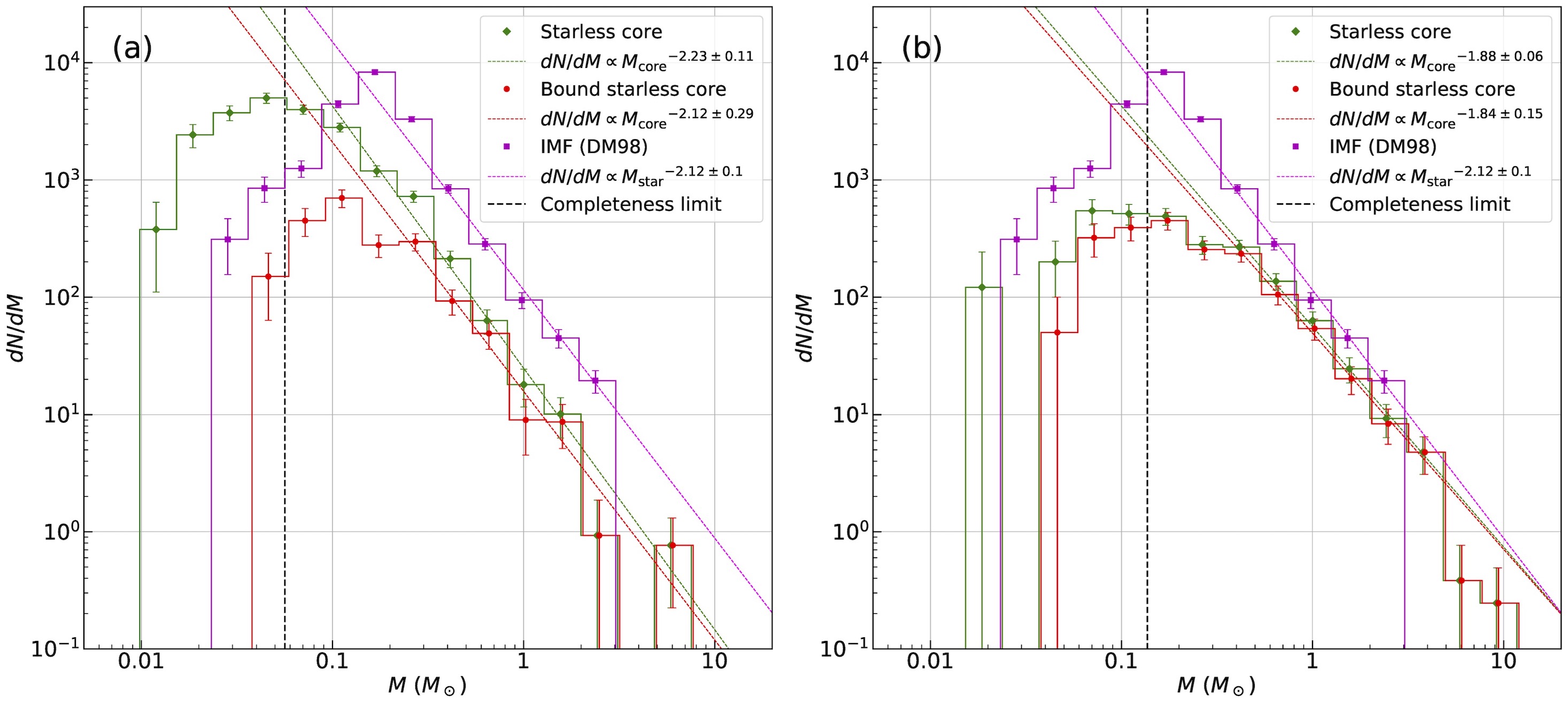
Figure 5: CMFs in the ONC region. The astrodendro’s parameters are(a) min_delta=2$\sigma$, min_value=2$\sigma$ and min_npix=60 and (b) min_delta=3$\sigma$, min_value=3$\sigma$ and min_npix=120, respectively. For comparison, we show the IMF derived by Da Rio et al. (2012) in both panels. The 90 % completeness limit is indicated with the vertical dashed lines. The error bars denote statistical errors.

Figure 5 (a) shows the CMFs toward ONC for all the starless cores and self-gravitating starless cores. For comparison, we show the stellar IMF in Figure 5. The shapes of the CMFs are similar to those of the stellar IMF. All CMFs have best-fit power-law indices of $\sim-$2 at the high-mass end. The CMFs for all starless cores and self-gravitating cores have the turnover masses of $\sim$0.05 $M_{\odot}$ (below the completeness limit) and $\sim$0.11 $M_{\odot}$, respectively, which are comparable to that of the IMF.

The results of the core identification depend on the adopted parameters of astrodendro. When we set min_delta=3$\sigma$, min_value=3$\sigma$ and min_npix=120 as the astrodendro parameters, we identified 270 starless cores and 224 bound starless cores. For comparison, we show the CMF derived with the above parameters in Figure 5 (b). The turnover masses of CMFs for starless cores and bound starless cores are $\sim$0.07 $M_{\odot}$ and $\sim$0.17 $M_{\odot}$, respectively. The differences in turnover masses of each CMF for different parameters are within 1 mass bin. Thus, we conclude that the dendrogram’s parameters do not change the turnover mass dramatically.

We calculated completeness by inserting into the map artificial cores that have a size corresponding to the beam size and FWHM line width of 3 channels (0.3 km/s). The total fluxes are calculated by assuming optically thin emission of C¹⁸O ($J$=1–0) with $T_{\mathrm{ex}}$ and $X_{\mathrm{C^{18}O}}$ derived in Figure 3 (a) and a central mass of each mass bin. We inserted one core to the data which position is random in trunks with avoiding the center overlaps observed cores. Then, we applied astrodendro to check if it is identified as a leaf. By repeating the procedure 1000 times for each mass bin, we calculated the detection probability. The 90 % completeness limits are shown as vertical dashed lines in Figure 5.

Ikeda & Kitamura (2009) derived the CMF in almost the same region using the same line C¹⁸O ($J$=1–0). They derived the turnover mass at $\sim$ 5 $M_{\odot}$, about 20 times larger than our value. They suggested that their turnover mass is an artifact of the poor angular resolution. The effect of angular resolution on the turnover mass is also discussed in Reid et al. (2010). There are two main differences between Ikeda & Kitamura (2009)’s and our analyses. One is the core identification method adopted. Ikeda & Kitamura (2009) used clumpfind algorithm (Williams et al., 1994) which tends to define a core as a structure larger than that identified with dendrogram since clumpfind algorithm allocates all pixels above a threshold to one of the cores. The more important difference is the angular resolution. In fact, applying the dendrogram to the NRO 45-m only data with 26″ resolution, Takemura et al. (2020) derived the turnover mass of about 0.5 M_⊙. This is about 5 times larger than that derived in this study. If the turnover mass depends only on the angular resolution, the artificial turnover mass obtained from the CARMA-NRO data is about 0.5/$(26/8)^{2}$ M_⊙ $\sim$ 0.05 M_⊙. On the other hand, our obtained turnover mass for the bound cores is about 0.1 M_⊙, larger than the value expected from the difference of the angular resolution (0.05 M_⊙). Thus, we believe that we constrain the true turnover mass for the bound cores reasonably well.

5 Discussion

The IMF in the ONC region is reproduced from our derived CMFs if it is assumed that (1) the star formation efficiency (SFE) of individual cores is constant over the whole mass range as discussed by Alves et al. (2007) and (2) the SFE of individual cores is 100%. However, assuming a SFE of 100% is unphysical, because mass-loss through a protostellar jet is a necessary part of the accretion process, with theoretical models, simulations and observations suggesting that $\sim 30$% of the accreting mass is lost that way (see the review by Pudritz et al., 2007). Furthermore, the feedback from outflows can also disperse part of the core mass, with the combined effect of jets and outflow feedback leading to a SFE of order 30% (e.g., Federrath et al., 2014). Thus, our results suggest that mass accretion onto the cores from a larger reservoir must be an ongoing process.

According to the standard scenario of star formation, the prestellar cores must be self-gravitating to initiate star formation. Assuming that all the self-gravitating starless cores ($\alpha_{\rm vir}<2$) form stars within a few free-fall times, we can evaluate the future star formation rate in this region. Assuming that the star formation timescale is about three times the free-fall time with the mean density of bound starless cores of 4$\times$10⁴ cm^-3, the future star formation rate is calculated to be 1$\times$10^-4 $M_{\odot}$ yr^-1. This is almost comparable to the recent star formation rate obtained in Section 2.3. Thus, our results seem to suggest that self-gravitating cores are likely to be direct progenitors of stars in the ONC region. However, we can not rule out the possibility of star formation from the gravitationally-unbound cores since the star formation rate would be only doubled even if all the starless cores form stars within a few free-fall time. Recent studies suggest that the majority of the cores are unbound (Maruta et al., 2010; Kirk et al., 2017), and such cores become gravitationally-bound or disperse eventually (Chen et al., 2020; Smullen et al., 2020).

If the accretion plays a role in determining the final stellar mass, we expect that our identified protostellar core population has a larger mean mass compared to that of the starless cores. The mean masses of starless cores and protostellar cores are $\sim$0.19 $M_{\odot}$ and $\sim$0.67 $M_{\odot}$, respectively. For protostellar core masses, we do not include the masses of protostars located inside. This larger mean mass for the protostellar cores is consistent with the idea that the starless cores gain significant gas from the surroundings during star formation. The importance of the mass accretion onto the cores is also pointed out by Dib et al. (2010).

6 Conclusions

In this Letter we have compared for the first time the CMF and IMF in the same region, which is located in the Orion Nebula Cluster. Determinations of the two functions with comparable sensitivities have revealed that the CMF has a turnover mass of $\sim$0.1 $M_{\odot}$, which is comparable to that of the IMF (see also Bontemps et al., 2001, for $\rho$ Oph). This seems to contradict the previous conclusion of a larger turnover mass of CMFs (e.g. Nutter & Ward-Thompson, 2007; Anathpindika, 2011). This difference may simply come from the difference in the angular resolutions of the observations.

To keep the slope of the CMF unchanged over time (so that the resultant IMF resembles the stellar IMF observed), the mass accretion rate onto individual cores should be proportional to $M_{\rm core}$ if the timescale of the accretion is more or less constant. The importance of the mass accretion appears to favor the competitive accretion scenario. However, according to the Bondi-Hoyle-Littleton accretion scenario the mass accretion rate is proportional to $M_{\rm core}^{2}$, and thus, the slopes of the CMFs can change with time (e.g., Goodwin et al., 2008). Numerical simulations also indicate that the actual accretion rates are significantly influenced by environments such as the global gravitational potential, and vary with time (e.g., Klessen, 2001; Girichidis et al., 2012). Our result indicates that the mass functions of the stellar seeds already resemble the IMF if the stellar seeds form by the gravitational collapse of the identified prestellar cores. Recent numerical simulations have pointed out the importance of mass accretion in the evolution of dense cores (Haugbølle et al., 2018; Padoan et al., 2014), leading to the inertial-inflow scenario. In contrast to both the core-collapse and the competitive-accretion models, the inertial-inflow model stresses the role of inertial turbulent flows in assembling the stellar mass from a large-scale mass reservoir (Padoan et al., 2020), even if the CMF and the IMF are very similar (Pelkonen et al., 2020), as found in this work.

Recent observations have detected the infall motions toward the prestellar cores (Contreras et al., 2018). A significant amount of parent core mass is likely to be blown out by the stellar feedback (e.g. Machida & Matsumoto, 2012). If the stellar feedback is important in determining the core mass, prestellar cores need to gain much more mass from the surroundings (Sanhueza et al., 2019).

Figure 1: (a) The C¹⁸O integrated intensity map and (b) the Herschel–Planck H₂ column density map toward the ONC region as a dashed rectangle. The identified C¹⁸O cores from this study and stars in the catalog of Da Rio et al. (2012) are plotted onto (a) and (b), respectively. In (a), the squares, circles, and crosses represent the protostellar cores, gravitationally bound starless cores, and unbound starless cores, respectively.

Figure 2: The histogram of the stellar age in the ONC region from Da Rio et al. (2012) with the DM98 model.

Figure 3: (a) The correlation between the mean C¹⁸O ($J$=1–0) integrated intensity and the mean Herschel–Planck H₂ column density in each projected core area. The solid line shows the best-fit function of optically thin LTE emission which is based on an abundance ratio of $X_{\mathrm{C^{18}O}}$=6.5$\times$10^-7 when $T_{\mathrm{ex}}$=20 K. (b) The relationship between the mass ratio, $M_{\mathrm{core}}/M_{\mathrm{projection}}$ and the Herschel– Planck H₂ column density.

Figure 4: Cartoon of dendrogram’s hierarchical structures of intensity focusing on a trunk and a leaf in position-velocity plane. The two arrows represent the intensity of a trunk and a leaf.

References

- Alves et al. (2007) Alves, J., Lombardi, M., & Lada, C. J. 2007, A&A, 462, L17, doi: 10.1051/0004-6361:20066389
- Anathpindika (2011) Anathpindika, S. 2011, New A, 16, 477, doi: 10.1016/j.newast.2011.03.002
- Ballesteros-Paredes et al. (2020) Ballesteros-Paredes, J., André, P., Hennebelle, P., et al. 2020, Space Sci. Rev., 216, 76, doi: 10.1007/s11214-020-00698-3
- Beaumont et al. (2013) Beaumont, C. N., Offner, S. S. R., Shetty, R., Glover, S. C. O., & Goodman, A. A. 2013, ApJ, 777, 173, doi: 10.1088/0004-637X/777/2/173
- Bonnell & Bate (2006) Bonnell, I. A., & Bate, M. R. 2006, MNRAS, 370, 488, doi: 10.1111/j.1365-2966.2006.10495.x
- Bontemps et al. (2001) Bontemps, S., André, P., Kaas, A. A., et al. 2001, A&A, 372, 173, doi: 10.1051/0004-6361:20010474
- Burkhart et al. (2013) Burkhart, B., Lazarian, A., Goodman, A., & Rosolowsky, E. 2013, ApJ, 770, 141, doi: 10.1088/0004-637X/770/2/141
- Chen et al. (2020) Chen, H. H.-H., Offner, S. S. R., Pineda, J. E., et al. 2020, arXiv e-prints, arXiv:2006.07325. https://arxiv.org/abs/2006.07325
- Cheng et al. (2018) Cheng, Y., Tan, J. C., Liu, M., et al. 2018, ApJ, 853, 160, doi: 10.3847/1538-4357/aaa3f1
- Clark et al. (2007) Clark, P. C., Klessen, R. S., & Bonnell, I. A. 2007, MNRAS, 379, 57, doi: 10.1111/j.1365-2966.2007.11896.x
- Contreras et al. (2018) Contreras, Y., Sanhueza, P., Jackson, J. M., et al. 2018, ApJ, 861, 14, doi: 10.3847/1538-4357/aac2ec
- Da Rio et al. (2012) Da Rio, N., Robberto, M., Hillenbrand, L. A., Henning, T., & Stassun, K. G. 2012, ApJ, 748, 14, doi: 10.1088/0004-637X/748/1/14
- D’Antona & Mazzitelli (1998) D’Antona, F., & Mazzitelli, I. 1998, New A, 134, 442
- Dib et al. (2010) Dib, S., Shadmehri, M., Padoan, P., et al. 2010, MNRAS, 405, 401, doi: 10.1111/j.1365-2966.2010.16451.x
- Federrath et al. (2014) Federrath, C., Schrön, M., Banerjee, R., & Klessen, R. S. 2014, ApJ, 790, 128, doi: 10.1088/0004-637X/790/2/128
- Furlan et al. (2016) Furlan, E., Fischer, W. J., Ali, B., et al. 2016, ApJS, 224, 5, doi: 10.3847/0067-0049/224/1/5
- Girichidis et al. (2012) Girichidis, P., Federrath, C., Banerjee, R., & Klessen, R. S. 2012, MNRAS, 420, 613, doi: 10.1111/j.1365-2966.2011.20073.x
- Goodwin et al. (2008) Goodwin, S. P., Nutter, D., Kroupa, P., Ward-Thompson, D., & Whitworth, A. P. 2008, A&A, 477, 823, doi: 10.1051/0004-6361:20078452
- Großschedl et al. (2018) Großschedl, J. E., Alves, J., Meingast, S., et al. 2018, A&A, 619, A106, doi: 10.1051/0004-6361/201833901
- Hartmann (2001) Hartmann, L. 2001, AJ, 121, 1030, doi: 10.1086/318770
- Haugbølle et al. (2018) Haugbølle, T., Padoan, P., & Nordlund, Å. 2018, ApJ, 854, 35, doi: 10.3847/1538-4357/aaa432
- Ikeda & Kitamura (2009) Ikeda, N., & Kitamura, Y. 2009, ApJ, 705, L95, doi: 10.1088/0004-637X/705/1/L95
- Kirk et al. (2017) Kirk, H., Friesen, R. K., Pineda, J. E., et al. 2017, ApJ, 846, 144, doi: 10.3847/1538-4357/aa8631
- Klessen (2001) Klessen, R. S. 2001, ApJ, 550, L77, doi: 10.1086/319488
- Klessen et al. (1998) Klessen, R. S., Burkert, A., & Bate, M. R. 1998, ApJ, 501, L205, doi: 10.1086/311471
- Klessen & Hennebelle (2010) Klessen, R. S., & Hennebelle, P. 2010, A&A, 520, A17, doi: 10.1051/0004-6361/200913780
- Kong (2019) Kong, S. 2019, ApJ, 873, 31, doi: 10.3847/1538-4357/aaffd5
- Kong et al. (2018) Kong, S., Arce, H. G., Feddersen, J. R., et al. 2018, ApJS, 236, 25, doi: 10.3847/1538-4365/aabafc
- Kroupa & Jerabkova (2019) Kroupa, P., & Jerabkova, T. 2019, Nature Astronomy, 3, 482, doi: 10.1038/s41550-019-0793-0
- Liu et al. (2018) Liu, M., Tan, J. C., Cheng, Y., & Kong, S. 2018, ApJ, 862, 105, doi: 10.3847/1538-4357/aacb7c
- Machida & Matsumoto (2012) Machida, M. N., & Matsumoto, T. 2012, MNRAS, 421, 588, doi: 10.1111/j.1365-2966.2011.20336.x
- Maruta et al. (2010) Maruta, H., Nakamura, F., Nishi, R., Ikeda, N., & Kitamura, Y. 2010, ApJ, 714, 680, doi: 10.1088/0004-637X/714/1/680
- McKee & Tan (2003) McKee, C. F., & Tan, J. C. 2003, ApJ, 585, 850, doi: 10.1086/346149
- Megeath et al. (2016) Megeath, S. T., Gutermuth, R., Muzerolle, J., et al. 2016, AJ, 151, 5, doi: 10.3847/0004-6256/151/1/5
- Menten et al. (2007) Menten, K. M., Reid, M. J., Forbrich, J., & Brunthaler, A. 2007, A&A, 474, 515, doi: 10.1051/0004-6361:20078247
- Motte et al. (1998) Motte, F., Andre, P., & Neri, R. 1998, A&A, 336, 150
- Motte et al. (2018) Motte, F., Nony, T., Louvet, F., et al. 2018, Nature Astronomy, 2, 478, doi: 10.1038/s41550-018-0452-x
- Nutter & Ward-Thompson (2007) Nutter, D., & Ward-Thompson, D. 2007, MNRAS, 374, 1413, doi: 10.1111/j.1365-2966.2006.11246.x
- Padoan et al. (2014) Padoan, P., Haugbølle, T., & Nordlund, Å. 2014, ApJ, 797, 32, doi: 10.1088/0004-637X/797/1/32
- Padoan et al. (2020) Padoan, P., Pan, L., Juvela, M., Haugbølle, T., & Nordlund, Å. 2020, ApJ, 900, 82, doi: 10.3847/1538-4357/abaa47
- Palla & Stahler (1999) Palla, F., & Stahler, S. W. 1999, ApJ, 525, 772, doi: 10.1086/307928
- Pelkonen et al. (2020) Pelkonen, V. M., Padoan, P., Haugbølle, T., & Nordlund, Å. 2020, arXiv e-prints, arXiv:2008.02192. https://arxiv.org/abs/2008.02192
- Pineda et al. (2009) Pineda, J. E., Rosolowsky, E. W., & Goodman, A. A. 2009, ApJ, 699, L134, doi: 10.1088/0004-637X/699/2/L134
- Pudritz et al. (2007) Pudritz, R. E., Ouyed, R., Fendt, C., & Brandenburg, A. 2007, in Protostars and Planets V, ed. B. Reipurth, D. Jewitt, & K. Keil, 277. https://arxiv.org/abs/astro-ph/0603592
- Reid et al. (2010) Reid, M. A., Wadsley, J., Petitclerc, N., & Sills, A. 2010, ApJ, 719, 561, doi: 10.1088/0004-637X/719/1/561
- Rosolowsky et al. (2008) Rosolowsky, E. W., Pineda, J. E., Kauffmann, J., & Goodman, A. A. 2008, ApJ, 679, 1338, doi: 10.1086/587685
- Sanhueza et al. (2019) Sanhueza, P., Contreras, Y., Wu, B., et al. 2019, ApJ, 886, 102, doi: 10.3847/1538-4357/ab45e9
- Shu et al. (1987) Shu, F. H., Adams, F. C., & Lizano, S. 1987, ARA&A, 25, 23, doi: 10.1146/annurev.aa.25.090187.000323
- Smullen et al. (2020) Smullen, R. A., Kratter, K. M., Offner, S. S. R., Lee, A. T., & Chen, H. H.-H. 2020, MNRAS, 497, 4517, doi: 10.1093/mnras/staa2253
- Takemura et al. (2020) Takemura, H., Nakamura, F., Ishii, S., et al. 2020, PASJ, submitted
- Vázquez-Semadeni et al. (2019) Vázquez-Semadeni, E., Palau, A., Ballesteros-Paredes, J., Gómez, G. C., & Zamora-Avilés, M. 2019, MNRAS, 490, 3061, doi: 10.1093/mnras/stz2736
- Wang et al. (2010) Wang, P., Li, Z.-Y., Abel, T., & Nakamura, F. 2010, ApJ, 709, 27, doi: 10.1088/0004-637X/709/1/27
- Williams et al. (1994) Williams, J. P., de Geus, E. J., & Blitz, L. 1994, ApJ, 428, 693, doi: 10.1086/174279
- Zinnecker (1982) Zinnecker, H. 1982, Annals of the New York Academy of Sciences, 395, 226, doi: 10.1111/j.1749-6632.1982.tb43399.x