Supplement to the paper
Cluster based inference for extremes of time series

Abstract

We continue the simulation study from section 3 of the main paper and provide additional simulation results in another model. Furthermore, we specify the variance example at the end of Section 2 by giving the concrete variance formulas. We verify three conditions of Theorem 2.3 for solutions to stochastic recurrence equations. Moreover, we state a modified version of the sliding block limit theorem from Drees and Neblung (2021) which is used for the proof of Theorem 2.3 of the main paper. Finally, we provide the proofs for equation (2.1), equation (A.4), Remark 2.2, Lemma A.2, Lemma A.9 (ii), Lemma A.10 and Lemma A.12 of the main paper.

black

, ,

To avoid confusion, we continue the section and figure numbering from the main article.

4 Further simulations.

In this section, we present additional simulation results about the finite sample performance of the projection based estimator ${\hat{\hat{p}}_{n,A}}$ and its competitors ${\hat{p}_{n,A}^{f}}$ and ${\hat{p}_{n,A}^{b}}$ of the cdf of $\Theta_{i}$. We keep the Monte Carlo setting (sample size, threshold, block length, number of Monte Carlo simulations) used in the paper.

In Section 3, among other things, the estimators are discussed in the GARCHt model for lag $i=10$, where ${\hat{\hat{p}}_{n,A}}$ performs best. Figure 3 shows the corresponding results for smaller lags, namely $i=1$ and $i=5$, respectively. Because ${\hat{\hat{p}}_{n,A}}$ and ${\hat{p}_{n,A}^{b}}$ have point mass at $0$, ${\hat{p}_{n,A}^{f}}$ typically has smallest bias among all estimators for small $|x|$, which is also reflected in the RMSE. In contrast, ${\hat{\hat{p}}_{n,A}}$ has smallest variance for most values of $x$ and this effect becomes more pronounced as the lag increases. Consequently, the projection based estimator outperforms the backward estimator, in particular as $i$ increases, and it has smallest RMSE for $|x|>0.3$ and all lags under consideration.

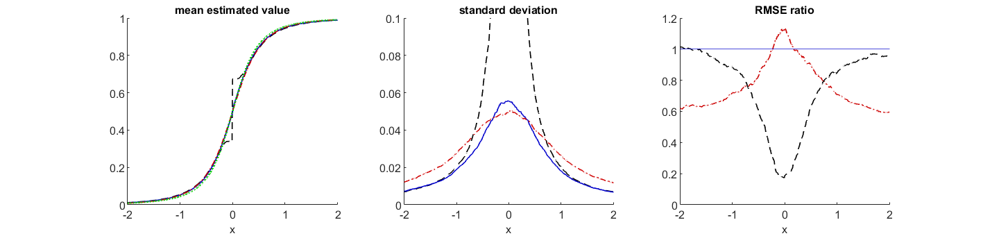
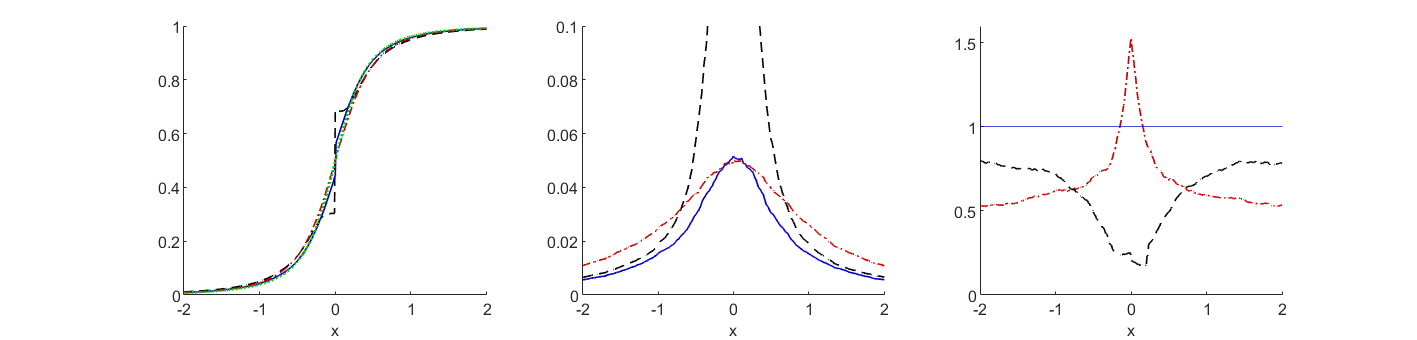
Figure 3: Mean (left), standard deviation (middle) and relative efficiency w.r.t.  ${\hat{\hat{p}}_{n,A}}$ (right), of ${\hat{\hat{p}}_{n,A}}$ (blue solid line), ${\hat{p}_{n,A}^{b}}$ (black dashed line) and ${\hat{p}_{n,A}^{f}}$ (red dashed-dotted line) in the GARCHt model for lags $i=1$ (top) and $i=5$ (bottom); the true cdf is indicated by the green dotted line.

While in the (asymmetric) SRE model (see Figure 2 in the paper for lag 1 and Figure 4 for lags $i\in\{5,10\}$) the variances of the three estimators behave similarly, the large bias, which is due to the influence of $D_{t}$, often dominates the RMSE, leading to an underperformance of ${\hat{\hat{p}}_{n,A}}$. This is particularly true for larger lags and negative $x$, while for $x>0$ and lag 10, ${\hat{\hat{p}}_{n,A}}$ has minimal RMSE.

Note that here the difference between the conditional distribution of the exceedances over the threshold $F_{|X|}^{\leftarrow}(0.95)$ and its limit distribution obscures almost all real differences between the estimators. It is thus instructive to compare, in addition, the performance of ${\hat{\hat{p}}_{n,A}}$, ${\hat{p}_{n,A}^{f}}$ and ${\hat{p}_{n,A}^{b}}$ interpreted as estimators of the pre-asymptotic cdf $P(X_{i}/|X_{0}|\leq x\mid|X_{0}|>F_{|X|}^{\leftarrow}(0.95))$ (rather than its limit $P\{\Theta_{i}\leq x\}$), like it was done in Davis et al. (2018) for the backward estimator. The corresponding plots for lag $i=1$ are shown in Figure 5. Of course, in the left plot only the true cdf has changed and the middle plot is exactly the same as in the bottom line of Figure 2, but the RMSE of the projection based estimator is much more strongly reduced than that of the forward estimators for $x$ not too close to 0. So, in this setting, ${\hat{\hat{p}}_{n,A}}$ overall performs best as an estimator of the pre-asymptotic cdf.

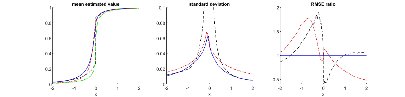
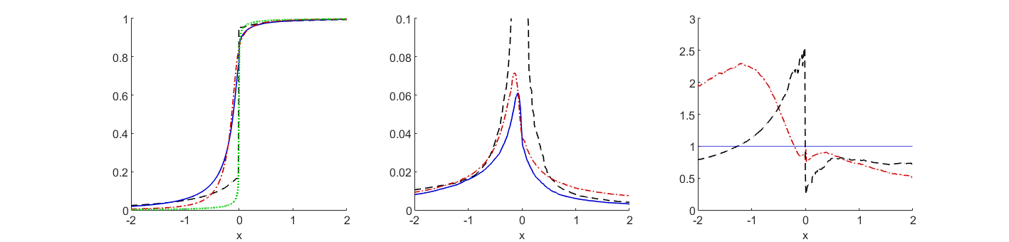
Figure 4: Mean (left), standard deviation (middle) and relative efficiency w.r.t.  ${\hat{\hat{p}}_{n,A}}$ (right), of ${\hat{\hat{p}}_{n,A}}$ (blue solid line), ${\hat{p}_{n,A}^{b}}$ (black dashed line) and ${\hat{p}_{n,A}^{f}}$ (red dashed-dotted line) in the SRE model for lags $i=5$ (top) and $i=10$ (bottom); the true cdf is indicated by the green dotted line.

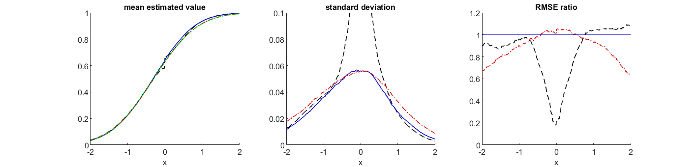
Figure 5: Mean (left), standard deviation (middle) and relative efficiency w.r.t.  ${\hat{\hat{p}}_{n,A}}$ (right), of ${\hat{\hat{p}}_{n,A}}$ (blue solid line), ${\hat{p}_{n,A}^{b}}$ (black dashed line) and ${\hat{p}_{n,A}^{f}}$ (red dashed-dotted line) as estimators of the pre-asymptotic cdf of $X_{i}/|X_{0}|$ given $|X_{0}|>F_{|X|}^{\leftarrow}(0.95)$ in the SRE model for lag $i=1$; the true cdf is indicated by the green dotted line.

In addition to the GARCHt and the SRE model, here we examine a model with trivial tail process:

• SV: Consider the stationary stochastic volatility model $X_{t}=\sigma_{t}\epsilon_{t},$ $t\in{\mathbb{Z}},$ with $\log(\sigma_{t})=0.9\log(\sigma_{t-1})+Z_{t}$ where $Z_{t}$ are i.i.d. standard normal random variables and $\epsilon_{t}$ are i.i.d. with Student’s $t_{2.6}$-distribution, independent of $(Z_{t})_{t\in Z}$. Then $(X_{t})_{t\in{\mathbb{Z}}}$ is a stationary regularly varying time series with $\alpha=2.6$ (cf. Davis et al. (2018), Section 4). Since the extremal behavior of $(X_{t})_{t\in{\mathbb{Z}}}$ is dominated by the i.i.d. heavy-tailed innovations $\epsilon_{t}$, we have $P\{\Theta_{i}=0\}=1$ for all $i\neq 0$, see Davis and Mikosch (2009).

Note that the conditions of Section 2 can only be fulfilled for the family of sets $(-\infty,x]$ if a neighborhood of 0 is omitted from the range of $x$-values. Nevertheless, here we present the results for the full range $[-2,2]$ (and lags $i\in\{1,10\}$) in Figure 6. For lag $i=1$, the projection based estimator performs best, but the loss of efficiency of the other estimators is less than 10%. In contrast, for $i=10$, the ${\hat{p}_{n,A}^{f}}$ has usually a moderately smaller RMSE than ${\hat{\hat{p}}_{n,A}}$, which in turn is preferable to ${\hat{p}_{n,A}^{b}}$ outside a tiny neighborhood of the origin.

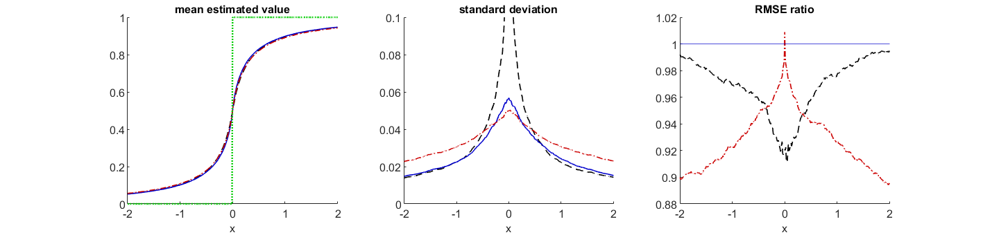
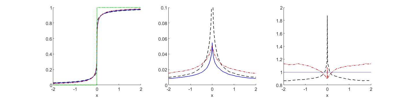
Figure 6: Mean (left), standard deviation (middle) and relative efficiency w.r.t.  ${\hat{\hat{p}}_{n,A}}$ (right), of ${\hat{\hat{p}}_{n,A}}$ (blue solid line), ${\hat{p}_{n,A}^{b}}$ (black dashed line) and ${\hat{p}_{n,A}^{f}}$ (red dashed-dotted line) in the SV model for lags $i=i$ (top) and $i=10$ (bottom); the true cdf is indicated by the green dotted line.

To sum up, usually the projection based estimator has the smallest variance, especially for larger lags. If pre-asymptotic probabilities significantly differ from the corresponding limit probabilities, ${\hat{\hat{p}}_{n,A}}$ may have a larger bias and RMSE than the forward estimator and sometimes also than the backward estimator. Overall, though, ${\hat{\hat{p}}_{n,A}}$ shows a more robust performance than both these estimators.

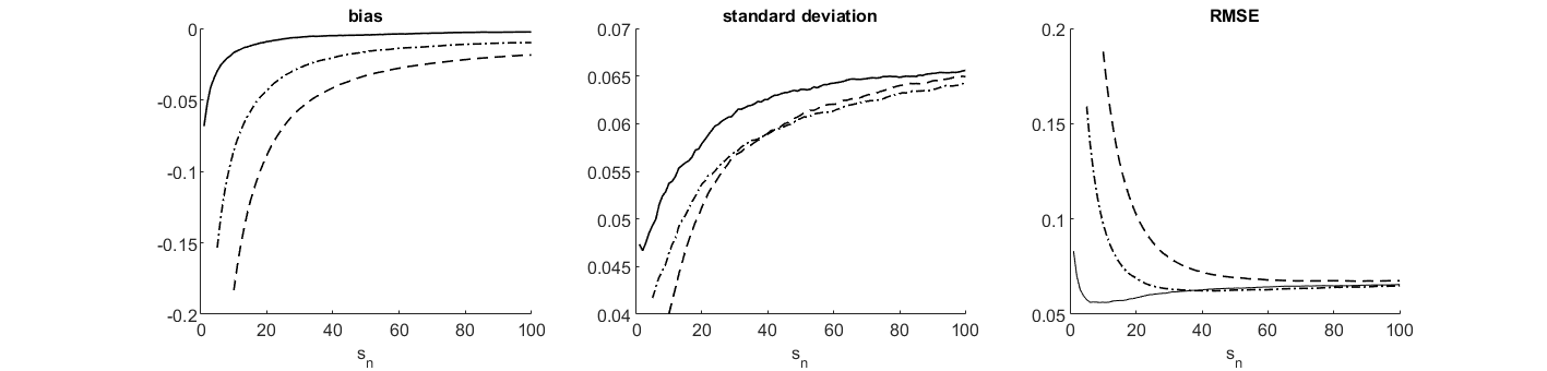
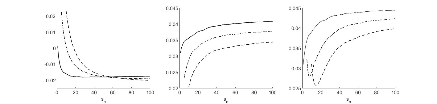
Figure 7: Bias (left), standard deviation (middle) and RMSE (right) of ${\hat{\hat{p}}_{n,A}}$ versus $s_{n}$, for lag $1$ (solid line), lag $5$ (dashed-dotted line) and lag $10$ (dashed line) with $x=0$ (top) and $x=1/2$ (bottom) in the GARCHt model.

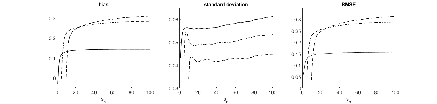
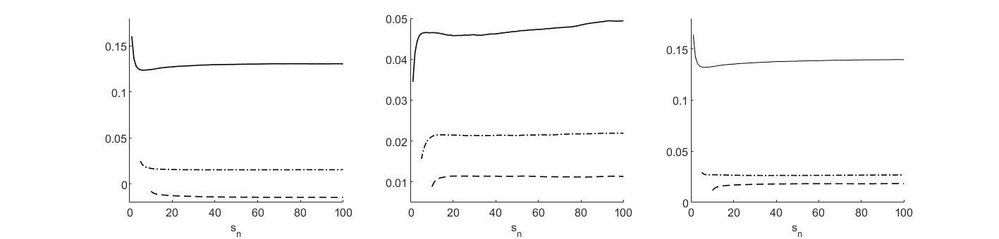
Figure 8: Bias (left), standard deviation (middle) and RMSE (right) of ${\hat{\hat{p}}_{n,A}}$ versus $s_{n}$, for lag $1$ (solid line), lag $5$ (dashed-dotted line) and lag $10$ (dashed line) with $x=0$ (top) and $x=1/2$ (bottom) in the SRE model.

Recall that in the definition of the projection based estimator one has to choose $s_{n}>i$ which determines the length of the blocks. Next, we examine the sensitivity of the estimators to changes of the block length.

If blocks are chosen too small than they do not capture the dependence structure of a typical cluster of extremes. Moreover, a point mass at 0 is introduced as an artefact of the artificial clipping of the cluster. On the other hand, if the block length is chosen too large, then almost independent clusters of large observations are compounded, which may lead to a bias and increase the variance, too.

Figure 7 shows the bias, the standard deviation and the RMSE of ${\hat{\hat{p}}_{n,A}}$ as function of $s_{n}$ for the lags $i\in\{1,5,10\}$ and $x\in\{0,0.5\}$ for the GARCHt model and Figure 8 does the same for the SRE model. For the GARCHt model, especially for larger lags, the estimator is clearly biased if $s_{n}$ is chosen too small (see top left plot in Figure 7), but for $s_{n}\geq 30$ the bias is small and the RMSE is quite stable. In the SRE model, in most cases the bias is caused by the deviation of the pre-asymptotic cdf from the limit cdf, discussed above. This negative bias happens to (partly) cancel a positive bias caused by too short a block out if $s_{n}$ is chosen small, leading to a very small RMSE. Apart from this very specific effect, the RMSE is again rather stable if $s_{n}$ is not too small. We thus recommend to choose the block length not too small (in particular for larger lags $i$), but unless an excessively large value is used, the performance of the estimator is not very sensitive to this tuning parameter.

To guide the selection of a reasonable value, a graph analogous to a Hill plot may be useful. In Figure 9, for a single a time series according to the GARCHt model, the value of ${\hat{\hat{p}}_{n,A}}$ is plotted versus $s_{n}$, for $A=(-\infty,-1]$ (left) and $A=(-\infty,1/2]$ (right). We suggest to choose $s_{n}$ in a range where the plots starts to stabilize, which in this case again leads to a value of about 30.

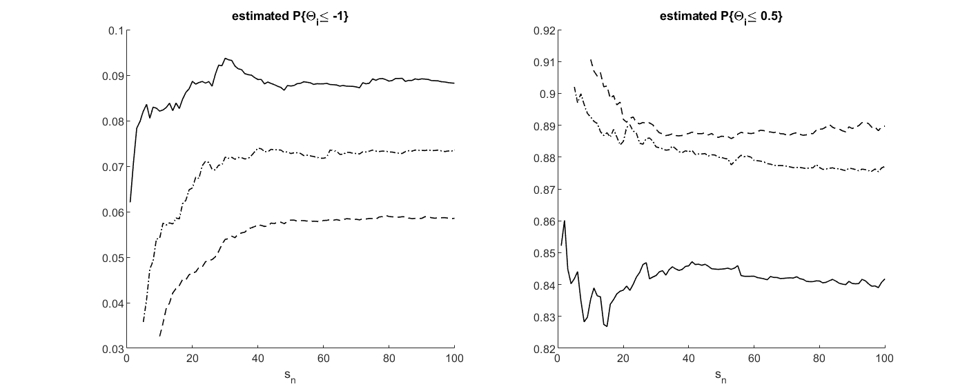
Figure 9: ${\hat{\hat{p}}_{n,A}}$ versus $s_{n}$ for a single realization of the GARCHt model for lag $1$ (solid line), lag $5$ (dashed-dotted line) and lag $10$ (dashed line) with $x=-1$ (left) and $x=0.5$ (right).

As always when the peaks-over-threshold approach is employed, all three estimators under consideration depend on the selected threshold $u_{n}$. So far, we have fixed this tuning parameter to the empirical $95\%$-quantile of $|X_{0}|$. Figure 10 displays the performance of all estimators for the cdf at $x=0.1$ in the GARCHt and the SRE model for lag 1 for different quantile levels. Unless the threshold is chosen very high, the performance of the projection based estimator and forward estimator seems quite stable. To a lesser extent, this is also true for the backward estimator, but here the performance deteriorates a bit faster. (Note that here we consider a set $A$ whose boundary $x$ is close to the origin, while the backward estimator is known to perform better for sets clearly bounded away from 0.)

To conclude, apparently the newly proposed estimator is quite insensitive to the choice of the block length, and it is not more sensitive to threshold selection than the direct forward estimator.

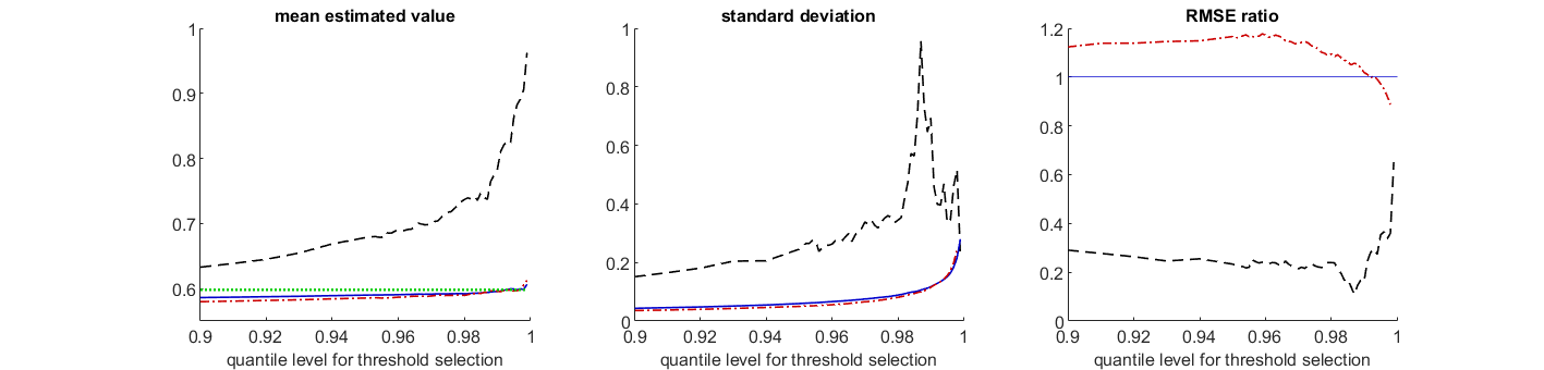
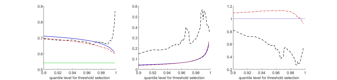
Figure 10: Mean (left), standard deviation (middle) and relative efficiency w.r.t.  ${\hat{\hat{p}}_{n,A}}$ (right) versus $F_{|X|}(u_{n})$, of ${\hat{\hat{p}}_{n,A}}$ (blue solid line), ${\hat{p}_{n,A}^{b}}$ (black dashed line) and ${\hat{p}_{n,A}^{f}}$ (red dashed-dotted line) in the GARCHt model (top) and in the SRE model (bottom) for lag $i=1$ and $x=0.1$; the true cdf is indicated by the green dotted line.

5 Example: comparison of asymptotic variances.

In this section we give further details for the calculation of the covariances in Example 2.4 of the main paper. Recall that we defined the process $W=(W_{t})_{t\in\mathbb{Z}}$ by

$$P\{W_{0}=a^{-1},W_{1}=-1,W_{t}=0,\,\forall t\notin\{0,1\}\}=p,$$ (5.1)

$$P\{W_{0}=1,W_{1}=b^{-1},W_{t}=0,\,\forall t\notin\{0,1\}\}=1-p$$ (5.2)

for some $a>1$, $b>1$ and $p=[0,1]$ and we set $\alpha=1$ and define $\Theta=(\Theta_{t})_{t\in\mathbb{Z}}$ such that $P^{\Theta}=(P^{W})^{RS}$, which results in

$$P\{\Theta\in D\} =E\left[\frac{\|W_{0}\|}{\|W_{0}\|+\|W_{1}\|}\mathds{1}_{D}\left(\frac{W}{\|W_{0}\|}\right)+\frac{\|W_{1}\|}{\|W_{0}\|+\|W_{1}\|}\mathds{1}_{D}\left(\frac{(W_{t+1})_{t\in\mathbb{Z}}}{\|W_{1}\|}\right)\right].$$ (5.3)

The specific choice $D=\{(y_{t})_{t\in\mathbb{Z}}|y_{-1}=a^{-1},y_{0}=-1,y_{t}=0\,\forall t\notin\{-1,0\}\}$ yields

$$P\{\Theta_{-1}=a^{-1},\Theta_{0}=-1,\Theta_{t}=0,\,\forall t\notin\{-1,0\}\} =p\frac{a}{a+1}.$$ (5.4)

Likewise, we obtain

$$P\{\Theta_{0}=1,\Theta_{1}=-a,\Theta_{t}=0,\,\forall t\notin\{0,1\}\}=p\frac{1}{a+1},$$ (5.5)

$$P\{\Theta_{-1}=b,\Theta_{0}=1,\Theta_{t}=0,\,\forall t\notin\{-1,0\}\}=(1-p)\frac{1}{1+b},$$ (5.6)

$$P\{\Theta_{0}=1,\Theta_{1}=b^{-1},\Theta_{t}=0,\,\forall t\notin\{0,1\}\}=(1-p)\frac{b}{1+b}.$$ (5.7)

According to Theorem 2.3, for sets $A$ such that its boundary is disjoint to $B:=\{-a,0,a^{-1},b^{-1},1,b\}$, the asymptotic variance of ${\hat{\hat{p}}_{n,A}}$ equals

$$Var\big{(}Z(A)-(p_{A}-\alpha d_{A})Z({\mathbb{R}})-\alpha^{2}d_{A}{Z_{\phi}}\big{)},$$

with $p_{A}=P\{\Theta_{i}\in A\}$ and $d_{A},Z$ and ${Z_{\phi}}$ given in Theorem 2.3 and (2.2).

Likewise, according to Davis et al. (2018), Theorem 3.1, for $A=(x,\infty)$ with $x\not\in B$, the asymptotic variance of ${\hat{p}_{n,A}^{b}}$ is given by

$$Var\big{(}\tilde{Z}(A)-p_{A}Z(\mathbb{R})+(\alpha^{2}{Z_{\phi}}-\alpha Z(\mathbb{R}))E[\log(\|\Theta_{i}\|)\mathds{1}_{A}(\Theta_{i})]\big{)}$$

where $(\tilde{Z},{Z_{\phi}},Z(\mathbb{R}))$ is a centered Gaussian process with covariance specified by the formulas in Theorem 2.3 and

$$Var(\tilde{Z}(A))=E\left[\sum_{j\in\mathbb{Z}}(\|\Theta_{j}\|^{\alpha}\wedge 1)\left(\frac{\|\Theta_{j-i}\|^{\alpha}}{\|\Theta_{j}\|^{\alpha}}\mathds{1}_{A}\left(\frac{\Theta_{j}}{\|\Theta_{j-i}\|}\right)\right)\left(\|\Theta_{-i}\|^{\alpha}\mathds{1}_{A}\left(\frac{\Theta_{0}}{\|\Theta_{-i}\|}\right)\right)\right],$$ (5.8)

$$Cov(\tilde{Z}(A),Z(\mathbb{R}))=E\left[\sum_{j\in\mathbb{Z}}(\|\Theta_{j}\|^{\alpha}\wedge 1)\left(\|\Theta_{-i}\|^{\alpha}\mathds{1}_{A}\left(\frac{\Theta_{0}}{\|\Theta_{-i}\|}\right)\right)\right]$$ (5.9)

$$Cov(\tilde{Z}(A),Z_{\phi})=E\left[\sum_{j\in\mathbb{Z}}(\|\Theta_{j}\|^{\alpha}\wedge 1)(\log(\|\Theta_{j}\|\vee 1)+\alpha^{-1})\|\Theta_{-i}\|^{\alpha}\mathds{1}_{A}\left(\frac{\Theta_{0}}{\|\Theta_{-i}\|}\right)\right].$$ (5.10)

Finally, from Davis et al. (2018), Theorem 3.1, it is known that in this setting the variance of the forward estimator ${\hat{p}_{n,A}^{f}}$ equals

$$\sum_{j\in\mathbb{Z}}E\left[(\|\Theta_{j}\|^{\alpha}\wedge 1)\left(p_{A}-\mathds{1}_{A}\left(\frac{\Theta_{j+i}}{\|\Theta_{j}\|}\right)\right)\left(p_{A}-\mathds{1}_{A}\left(\Theta_{i}\right)\right)\right].$$ (5.11)

All these expectations can be easily calculated numerically, since the spectral tail process $(\Theta_{t})_{t\in{\mathbb{Z}}}$ vanishes for $|t|>1$ and its distribution is discrete with just 4 points of mass.

Note that the asymptotic variances of the backward estimator and the projection based estimator with known $\alpha$ can be calculated likewise, by omitting all terms involving $d_{A}$ or $E[\log(\|\Theta_{i}\|)\mathds{1}_{\{\Theta_{i}\in A\}}]$.

6 Verification of (BC), (BC’) and (M) (i) for solutions to stochastic recurrence equations.

In Subsection 2.1 of the main paper we discussed stationary solutions to stochastic recurrence equations

$$X_{t}=C_{t}X_{t-1}+D_{t},\quad t\in{\mathbb{Z}},$$ (6.1)

where $C_{t}$ are random $d\times d$-matrices with non-negative entries and $D_{t}$ are $[0,\infty)^{d}$-valued random vectors so that $(C_{t},D_{t})$, $t\in{\mathbb{Z}}$ are i.i.d. The Conditions (SRE) and (SRE’) have been used to conclude the existence of a stationary regular varying solution and that $(X_{t})_{t\in\mathbb{Z}}$ is an aperiodic, positive Harris recurrent, $P^{X_{0}}$-irreducible Feller process. Recall

$$X_{t}=\Pi_{1,t}X_{0}+R_{t}$$ (6.2)

where $\Pi_{j,k}:=C_{k}\cdots C_{j}$ and $R_{t}:=\sum_{j=1}^{t}\Pi_{j+1,t}D_{j}$ are independent of $X_{0}$.

Here we give more details why Conditions (BC), (BC’) and (M) (i) are satisfied in this setting. As in the paper, $\|\cdot\|$ denotes both the Euclidean norm of a vector and the corresponding operator norm of a matrix. Recall that for all $q\in(0,\alpha)$ one has for sufficient large $m$

$$\kappa:=E(\|\Pi_{1,m}\|^{q})<1$$

and

$$E[\|\Pi_{1,k}\|^{q}]\leq c_{m}\tilde{\kappa}^{k}$$ (6.3)

for all $k\in\mathbb{N}$, some $c_{m}>0$ and $\tilde{\kappa}:=\kappa^{1/m}<1$.

Fix some $c\in(0,1]$ and let $v_{n,c}:=P\{\|X_{0}\|>cu_{n}\}$. In view of (6.2)

$$P(\|X_{k}\|>cu_{n}\mid\|X_{0}\|>cu_{n})$$ (6.4)

$$\leq\frac{1}{v_{n,c}}P\{\|X_{0}\|>cu_{n},\|R_{k}\|+\|\Pi_{1,k}X_{0}\|>cu_{n}\}$$ (6.5)

$$\leq\frac{1}{v_{n,c}}\Big{(}P\Big{\{}\|X_{0}\|>cu_{n},\|R_{k}\|>\frac{cu_{n}}{2}\Big{\}}+P\Big{\{}\|X_{0}\|>cu_{n},\|\Pi_{1,k}\|\|X_{0}\|>\frac{cu_{n}}{2}\Big{\}}\Big{)}$$ (6.6)

$$=P\Big{\{}\|R_{k}\|>\frac{cu_{n}}{2}\Big{\}}+\frac{1}{v_{n,c}}\int_{cu_{n}}^{\infty}P\Big{\{}\|\Pi_{1,k}\|>\frac{cu_{n}}{2t}\Big{\}}P^{\|X_{0}\|}(dt).$$ (6.7)

Since we assume that $C$ and $D$ only have non-negative entries, the first summand can be bounded by $P\{\|X_{k}\|>cu_{n}/2\}=v_{n,c/2}$. For the second term, the generalized Markov inequality and (6.3) yield

$$P\Big{\{}\|\Pi_{1,k}\|>\frac{cu_{n}}{2t}\Big{\}}\leq E[\|\Pi_{1,k}\|^{q}]\Big{(}\frac{2t}{cu_{n}}\Big{)}^{q}\leq c_{m}\tilde{\kappa}^{k}\Big{(}\frac{2t}{cu_{n}}\Big{)}^{q}.$$ (6.8)

Hence,

$$\frac{1}{v_{n,c}}\int_{cu_{n}}^{\infty}P\Big{\{}\|\Pi_{1,k}\|>\frac{cu_{n}}{2t}\Big{\}}P^{\|X_{0}\|}(dt)\leq 2^{q}c_{m}\tilde{\kappa}^{k}E\bigg{(}\Big{(}\frac{\|X_{0}\|}{cu_{n}}\Big{)}^{q}\Big{|}\|X_{0}\|>cu_{n}\bigg{)}$$ (6.9)

for all $k\in\mathbb{N}$. To sum up, we have shown

$$P\{\|X_{k}\|>cu_{n}\mid\|X_{0}\|>cu_{n}\}\leq v_{n,c/2}+2^{q}c_{m}\tilde{\kappa}^{k}E\bigg{(}\Big{(}\frac{\|X_{0}\|}{cu_{n}}\Big{)}^{q}\Big{|}\|X_{0}\|>cu_{n}\bigg{)}=:e_{n,c}(k)$$ (6.10)

which is (2.11) in the main paper.

Because of regular variation of $\|X_{0}\|$, $q<\alpha$ and $r_{n}v_{n}\to 0$, we have $E((\|X_{0}\|/cu_{n})^{q}\mid\|X_{0}\|>cu_{n})\to E(\|Y_{0}\|^{q})$ and $r_{n}v_{n,c/2}=r_{n}v_{n}(v_{n,c/2}/v_{n})\to 0$. Therefore

$$e_{\infty,c}(k)=\lim_{n\to\infty}e_{n,c}(k)=2^{q}c_{m}\tilde{\kappa}^{k}E(\|Y_{0}\|^{q})<\infty$$

and

$$\sum_{k=1}^{r_{n}}e_{n,c}(k) =r_{n}v_{n,c/2}+2^{q}c_{m}E\bigg{(}\Big{(}\frac{\|X_{0}\|}{cu_{n}}\Big{)}^{q}\Big{|}\|X_{0}\|>cu_{n}\bigg{)}\sum_{k=1}^{r_{n}}\tilde{\kappa}^{k}$$ (6.11)

$$\rightarrow 2^{q}c_{m}E(\|Y_{0}\|^{q})\Big{(}\frac{1}{1-\tilde{\kappa}}-1\Big{)}=\sum_{k=1}^{\infty}e_{\infty,c}(k)<\infty,$$ (6.12)

i.e. condition (BC).

Next observe that, for $p\in(0,\alpha)$, from the drift condition $E(\|X_{1}\|^{p}\mid X_{0}=y)\leq\beta\|y\|^{p}+b$, i.e. Assumption 2.1 (iii) of Kulik et al. (2019) which has been established in Subsection 2.1 with some $\beta\in(0,1)$ and some $b>0$, one may conclude by induction that $E(\|X_{k}\|^{p}\mid X_{0}=y)\leq\beta^{k}\|y\|^{p}+b/(1-\beta)$ (Douc et al. (2018), Proposition 14.1.8). For all $p,\tilde{p}>0$ such that $p+\tilde{p}<\alpha$, it follows

$$E\Big{(} \Big{(}\frac{\|X_{k}\|}{u_{n}}\Big{)}^{p}\Big{(}\frac{\|X_{0}\|}{u_{n}}\Big{)}^{\tilde{p}}\mathds{1}_{\{\|X_{k}\|>u_{n}\}}\ \Big{|}\ \|X_{0}\|>u_{n}\Big{)}$$ (6.13)

$$\leq v_{n}^{-1}\int_{u_{n}}^{\infty}u_{n}^{-(p+\tilde{p})}E(\|X_{k}\|^{p}\mid\|X_{0}\|=y)\|y\|^{\tilde{p}}\ P^{\|X_{0}\|}(\mathrm{d}y)$$ (6.14)

$$\leq\beta^{k}E\Big{(}\Big{(}\frac{\|X_{0}\|}{u_{n}}\Big{)}^{p+\tilde{p}}\ \Big{|}\ \|X_{0}\|>u_{n}\Big{)}+\frac{b}{1-\beta}u_{n}^{-p}E\Big{(}\Big{(}\frac{\|X_{0}\|}{u_{n}}\Big{)}^{\tilde{p}}\ \Big{|}\ \|X_{0}\|>u_{n}\Big{)}$$ (6.15)

$$\leq 2\beta^{k}E(\|Y_{0}\|^{p+\tilde{p}})+\frac{2b}{1-\beta}u_{n}^{-p}E(\|Y_{0}\|^{\tilde{p}})$$ (6.16)

for sufficiently large $n$.

Define $\psi(x):=\max(\log\|x\|,\mathds{1}_{[1,\infty)}(\|x\|))$, which for all $p>0$ can be bounded in absolute value by $\tilde{c}_{p}\|x\|^{p}\mathds{1}_{\{\|x\|>1\}}$ for some constant $\tilde{c}_{p}$. The uniform moment bound (6.16) readily shows that the random variables $\psi(X_{0}/u_{n})\psi(X_{k}/u_{n})/v_{n}$ are uniformly integrable, so that the definition of the tail process yields

$$e^{\prime}_{n}(k):=E(\psi(X_{0}/u_{n})\psi(X_{k}/u_{n})\mid\|X_{0}\|>u_{n})\to e^{\prime}_{\infty}(k):=E[\psi(Y_{0})\psi(Y_{k})]<\infty$$

for all $k\in\mathbb{N}$. Moreover, the representation of the forward tail process $Y_{k}=\|Y_{0}\|\Theta_{0}\Pi_{1,k}$ and (6.3) show that the $e^{\prime}_{\infty}(k)$ are summable:

$$\sum_{k=1}^{\infty}e^{\prime}_{\infty}(k)\leq\tilde{c}_{q/2}^{2}E[\|Y_{0}\|^{q}]\sum_{k=1}^{\infty}E[\|\Pi_{1,k}\|^{q}]\leq\tilde{c}_{q/2}^{2}c_{m}E[\|Y_{0}\|^{q}]\sum_{k=1}^{\infty}\tilde{\kappa}^{k}<\infty.$$

Hence, for all $\varepsilon>0$, one can find some $L\in{\mathbb{N}}$ such that $\sum_{k=L+1}^{\infty}e^{\prime}_{\infty}(k)<\varepsilon$. Using (6.16) and convergence (2.10), one may conclude for sufficiently large $L^{\prime}\geq L$

$$\limsup_{n\to\infty}\Big{|}\sum_{k=1}^{r_{n}}e^{\prime}_{n}(k)-\sum_{k=1}^{\infty}e^{\prime}_{\infty}(k)\Big{|} \leq\limsup_{n\to\infty}\Big{|}\sum_{k=1}^{L^{\prime}}e^{\prime}_{n}(k)-\sum_{k=1}^{L^{\prime}}e^{\prime}_{\infty}(k)\Big{|}+2\varepsilon=2\varepsilon.$$ (6.17)

Let $\varepsilon$ tend to 0 to obtain (BC’).

Finally, (6.16) with $p\in(\alpha(1+\delta)/(1+\zeta),\alpha)$, $\delta<\zeta$, and $\tilde{p}\in(0,\alpha-p)$ shows that the sum on the left-hand side of Condition (M) (i) can be bounded by a multiple of

$$\sum_{k=1}^{r_{n}}\Big{(}\beta^{k}E[\|Y_{0}\|^{p+\tilde{p}}]+u_{n}^{-p}E[\|Y_{0}\|^{\tilde{p}}]\Big{)}^{1/(1+\delta)}$$ (6.18)

$$\leq\sum_{k=1}^{r_{n}}(\beta^{1/(1+\delta)})^{k}(E[\|Y_{0}\|^{p+\tilde{p}}])^{1/(1+\delta)}+r_{n}u_{n}^{-p/(1+\delta)}(E[\|Y_{0}\|^{\tilde{p}}])^{1/(1+\delta)}$$ (6.19)

$$={\hbox{O}}(1),$$ (6.20)

provided $r_{n}^{1+\zeta}v_{n}$ is bounded, because $u_{n}$ is of larger order than $v_{n}^{\eta-1/\alpha}$ for all $\eta>0$.

7 Modified sliding blocks limit theorem.

In this section we present a slightly modified version of a limit theorem for unbounded functions of sliding blocks introduced by Drees and Neblung (2021) (D&N), Theorem 2.4, which is applied in the proof of Theorem 2.3 of the main paper. To this end, assume that $(X_{n,i})_{1-s_{n}\leq i\leq n+s_{n},n\in\mathbb{N}}$ is a triangular array of row-wise stationary random variables, consider a set $\mathcal{G}$ of functionals defined on vectors of arbitrary length and define $W_{n,j}:=(X_{n,j-s_{n}},...,X_{n,j+s_{n}})$ for some sequence $s_{n}$,

$$V_{n,i}(g) :=\frac{1}{b_{n}(g)}\sum_{j=1}^{r_{n}}g(W_{n,(i-1)r_{n}+j}),$$ (7.1)

$$\tilde{V}_{n,i}(g) :=\frac{1}{b_{n}(g)}\sum_{j=1}^{r_{n}-l_{n}}g(W_{n,(i-1)r_{n}+j}),$$ (7.2)

$$\bar{Z}_{n}(g) :=\frac{1}{\sqrt{p_{n}}b_{n}(g)}\sum_{j=1}^{n}\left(g(W_{n,j})-Eg(W_{n,j})\right),$$ (7.3)

$$Z_{n}(g) :=\frac{1}{\sqrt{p_{n}}}\sum_{i=1}^{\lfloor n/r_{n}\rfloor}\left(V_{n,i}(g)-EV_{n,i}(g)\right),\qquad g\in\mathcal{G},$$ (7.4)

and $p_{n}:=P\{\exists g\in\mathcal{G}:V_{n}(g)\neq 0\}$ for some suitable sequence $r_{n}={\hbox{o}}(n)$; here $V_{n}$ denotes a random variable with the same distribution as $V_{n,1}$. Moreover, we use the following conditions taken from Section 2 and Appendix A of D&N:

• $(X_{n,i})_{1\leq i\leq n}$ is stationary for all $n\in\mathbb{N}$.

• The sequences $l_{n},r_{n},s_{n}\in{\mathbb{N}}$, $p_{n}$, and $b_{n}(g)>0$, $g\in{\mathcal{G}}$, satisfy $s_{n}\leq l_{n}={\hbox{o}}(r_{n})$, $r_{n}={\hbox{o}}(n)$, $p_{n}\to 0$ and $r_{n}={\hbox{o}}\big{(}\sqrt{p_{n}}\inf_{g\in{\mathcal{G}}}b_{n}(g)\big{)}$.

• The processes $V_{n}$, $n\in{\mathbb{N}}$, are separable.

• $m_{n}\beta_{n,l_{n}-(2s_{n}+1)}^{X}\to 0$ for $m_{n}:=\lfloor n/r_{n}\rfloor$.

• There exists a function $c:{\mathcal{G}}^{2}\to{\mathbb{R}}$ such that

  $$\frac{m_{n}}{p_{n}}Cov\left(V_{n}(g),V_{n}(h)\right)\rightarrow c(g,h),\qquad\forall\,g,h\in\mathcal{G}.$$ (7.5)

• $\Delta_{n}:=V_{n}-\tilde{V}_{n}$ satisfies

  (i) $\displaystyle E\left[(\Delta_{n}(g)-E[\Delta_{n}(g)])^{2}\mathds{1}_{\left\{|\Delta_{n}(g)-E[\Delta_{n}(g)]|\leq\sqrt{p_{n}}\right\}}\right]={\hbox{o}}\left(p_{n}/m_{n}\right),\qquad\forall\,g\in\mathcal{G},$

  (ii) $\displaystyle P\left\{|\Delta_{n}(g)-E[\Delta_{n}(g)]|>\sqrt{p_{n}}\right\}={\hbox{o}}\left(1/m_{n}\right),\qquad\forall\,g\in\mathcal{G}.$

  (iii) $\displaystyle E\left[(\Delta_{n}(g)-E[\Delta_{n}(g)])\mathds{1}_{\left\{|\Delta_{n}(g)-E[\Delta_{n}(g)]|\leq\tau\sqrt{p_{n}}\right\}}\right]=\hbox{o}\left(\sqrt{p_{n}}/m_{n}\right),\qquad\forall g\in\mathcal{G}$ for some $\tau>0$.

• $\displaystyle E\left[(V_{n}(g)-E[V_{n}(g)])^{2}\mathds{1}_{\left\{|V_{n}(g)-E[V_{n}(g)]|>\epsilon\sqrt{p_{n}}\right\}}\right]={\hbox{o}}\left(p_{n}/m_{n}\right),\quad\forall\,g\in\mathcal{G},\epsilon>0.$

• There exists a semi-metric $\rho$ on $\mathcal{G}$ such that $\mathcal{G}$ is totally bounded and

  $$\lim_{\delta\downarrow 0}\limsup_{n\to\infty}\sup_{g,h\in\mathcal{G},\rho(g,h)<\delta}\frac{m_{n}}{p_{n}}E\big{[}(V_{n}(g)-V_{n}(h))^{2}\big{]}=0.$$ (7.6)

• $$\lim_{\delta\downarrow 0}\limsup_{n\to\infty}\int_{0}^{\delta}\sqrt{\log N_{[\cdot]}(\epsilon,\mathcal{G},L_{2}^{n})}\,d\epsilon=0,$$ (7.7)

  where $N_{[\cdot]}(\epsilon,\mathcal{G},L_{2}^{n})$ denotes the $\epsilon$-bracketing number of ${\mathcal{G}}$ w.r.t. $L_{2}^{n}$, i.e. the smallest number $N_{\epsilon}$ such that for each $n\in\mathbb{N}$ there exists a partition $(\mathcal{G}_{n,k}^{\epsilon})_{1\leq k\leq N_{\epsilon}}$ of $\mathcal{G}$ satisfying

  $$\frac{m_{n}}{p_{n}}E^{*}\Big{[}\sup_{g,h\in\mathcal{G}_{n,k}^{\epsilon}}(V_{n}(g)-V_{n}(h))^{2}\Big{]}\leq\epsilon^{2},\qquad\forall 1\leq k\leq N_{\epsilon}.$$ (7.8)

  (Here $E^{*}$ denotes the outer expectation.)

• Denote by $N(\epsilon,\mathcal{G},d_{n})$ the $\epsilon$-covering number of ${\mathcal{G}}$ w.r.t. the random semi-metric

  $$d_{n}(g,h)=\bigg{(}\frac{1}{p_{n}}\sum_{i=1}^{m_{n}}(V_{n,i}^{*}(g)-V_{n,i}^{*}(h))^{2}\bigg{)}^{1/2}$$ (7.9)

  with $V_{n,i}^{*}$, $1\leq i\leq m_{n}$, independent copies of $V_{n,1}$, i.e. $N(\epsilon,\mathcal{G},d_{n})$ is the smallest number of balls with respect to $d_{n}$ with radius $\epsilon$ that is needed to cover $\mathcal{G}$. We assume

  $$\lim_{\delta\downarrow 0}\limsup_{n\to\infty}P^{*}\bigg{\{}\int_{0}^{\delta}\sqrt{\log(N(\epsilon,\mathcal{G},d_{n}))}d\epsilon>\tau\bigg{\}}=0,\qquad\forall\tau>0.$$ (7.10)

Condition ($\Delta$) is always fulfilled if

$$E\left[(\Delta_{n}(g))^{2}\right]=\hbox{o}\left(p_{n}/m_{n}\right),\quad\forall g\in\mathcal{G}.$$ (7.11)

Then we can modify Theorem 2.4 of D&N as follows.

Theorem 7.1.

• Suppose the conditions (A1), (A2), (D0), (MX) and (C) are met. Moreover, assume condition (L) is satisfied and

  $$E\bigg{[}\bigg{(}\sum_{i=1}^{r_{n}}|g(W_{n,i})|\bigg{)}^{2}\bigg{]}={\hbox{O}}\bigg{(}\frac{p_{n}b_{n}^{2}(g)}{m_{n}}\bigg{)},\quad\forall\,g\in{\mathcal{G}}.$$ (7.12)

  Then the fidis of $(Z_{n}(g))_{g\in\mathcal{G}}$ and of $(\bar{Z}_{n}(g))_{g\in\mathcal{G}}$ converge to the fidis of the Gaussian process $(Z(g))_{g\in\mathcal{G}}$ defined in Theorem 2.1 of D&N.

• If, in addition, $g_{\max}=\sup_{g\in\mathcal{G}}|g|$ is measurable, $b_{n}(g)=b_{n}$ is the same for all $g\in{\mathcal{G}}$, (7.12) holds for $g=g_{\max}$ and the conditions (D1) and (D2) or the conditions (D1) and (D3) are fulfilled, then the processes $(Z_{n}(g))_{g\in\mathcal{G}}$ and $(\bar{Z}_{n}(g))_{g\in\mathcal{G}}$ converge weakly to $(Z(g))_{g\in\mathcal{G}}$ uniformly.

So, in comparison with Theorem 2.4 of D&N, basically condition (2.8) in that paper, which is the analog to (7.12) with some exponent strictly greater than 2, is replaced with the weaker condition (7.12), a weak technical condition is omitted, and as a compensation condition (L) is added.

Proof of Theorem 7.1.

The proof is basically the same as for Theorem 2.4 in D&N. We apply Theorem A.1 of D&N to the observations $X^{\prime}_{n,t}:=X_{n,t-s_{n}}$, $1\leq t\leq n^{\prime}:=n+2s_{n}$, and block lengths $s^{\prime}_{n}:=2s_{n}+1$ and $l_{n}^{\prime}:=l_{n}+s_{n}+1$ to establish fidi-convergence of $(Z_{n}(g))_{g\in\mathcal{G}}$. Only Condition ($\Delta$) must be verified, because (L) is assumed and the remaining conditions follow as in the proof of Theorem 2.1 of D&N. Since

$$E\bigg{[}\bigg{(}\sum_{i=1}^{r_{n}}|g(W_{n,i})|\Bigg{)}^{2}\bigg{]} \geq\sum_{j=1}^{\lfloor r_{n}/l_{n}\rfloor}E\bigg{[}\bigg{(}\sum_{i=1}^{l_{n}}|g(W_{n,(j-1)l_{n}+i})|\bigg{)}^{2}\bigg{]}$$ (7.13)

$$=\lfloor r_{n}/l_{n}\rfloor E\bigg{[}\bigg{(}\sum_{i=1}^{l_{n}}|g(W_{n,i})|\bigg{)}^{2}\bigg{]},$$ (7.14)

(7.12) and $l_{n}={\hbox{o}}(r_{n})$ imply

$$E(\Delta_{n}(g)^{2}) \leq\frac{1}{b_{n}^{2}(g)}E\bigg{[}\bigg{(}\sum_{i=1}^{l_{n}}|g(W_{n,i})|\bigg{)}^{2}\bigg{]}\leq\frac{1}{b_{n}^{2}(g)\lfloor r_{n}/l_{n}\rfloor}E\bigg{[}\bigg{(}\sum_{i=1}^{r_{n}}|g(W_{n,i})|\bigg{)}^{2}\bigg{]}$$ (7.15)

$$={\hbox{O}}\bigg{(}\frac{l_{n}}{r_{n}b_{n}^{2}(g)}\frac{p_{n}b_{n}^{2}(g)}{m_{n}}\bigg{)}={\hbox{o}}\bigg{(}\frac{p_{n}}{m_{n}}\bigg{)}.$$ (7.16)

Hence, equation (7.11) holds, which in turn yields ($\Delta$). Now, the convergence of the fidis of $(Z_{n}(g))_{g\in\mathcal{G}}$ follows from Theorem A.1 of D&N. Similarly,

$$E\Big{(}(\bar{Z}_{n}(g)-Z_{n}(g))^{2}\Big{)}\leq\frac{1}{p_{n}b_{n}^{2}(g)}E\bigg{[}\bigg{(}\sum_{j=r_{n}m_{n}+1}^{n-s_{n}}|g(W_{n,j})|\bigg{)}^{2}\bigg{]}={\hbox{O}}\bigg{(}\frac{1}{m_{n}}\bigg{)}\to 0,$$ (7.17)

so that the fidi-convergence of $(\bar{Z}_{n}(g))_{g\in\mathcal{G}}$ follows, too.

Part (ii) of the assertion can be concluded by the same arguments as in the proof of Theorem 2.4 of D&N. ∎

8 Proof of (2.1) and (A.4).

First we want to establish (2.1) of the paper, i.e. the convergence

$$E(g_{A}(W_{n,0})\mid\|X_{0}\|>u_{n})\to E\big{(}g_{A}(Y)\big{)}=E\Big{(}\|\Theta\|_{\alpha}^{-\alpha}\sum_{h\in{\mathbb{Z}}}\|\Theta_{h}\|^{\alpha}\mathds{1}_{A}(\Theta_{h+i}/\|\Theta_{h}\|)\Big{)}$$ (8.1)

for $g_{A}:l_{\alpha}\to[0,1]$,

$$g_{A}\big{(}(w_{h})_{h\in\mathbb{Z}}\big{)} :=\frac{\mathds{1}_{\{\|w_{0}\|>1\}}}{\sum_{h\in\mathbb{Z}}\|w_{h}\|^{\alpha}}\sum_{h\in\mathbb{Z}}\|w_{h}\|^{\alpha}\mathds{1}_{A}\Big{(}\frac{w_{h+i}}{\|w_{h}\|}\Big{)}$$ (8.2)

and $W_{n,t}:=(X_{n,t+h})_{|h|\leq s_{n}}$, $X_{n,t}:=X_{t}/u_{n}$. To this end, we define the approximating functions $g_{A}^{(m)}:l_{\alpha}\to\mathbb{R}$,

$$g_{A}^{(m)}\big{(}(w_{h})_{h\in\mathbb{Z}}\big{)} :=\frac{\mathds{1}_{\{\|w_{0}\|>1\}}}{\sum_{|h|\leq m}\|w_{h}\|^{\alpha}}\sum_{|h|\leq m}\|w_{h}\|^{\alpha}\mathds{1}_{A}\Big{(}\frac{w_{h+i}}{\|w_{h}\|}\Big{)}$$ (8.3)

for all $m\in\mathbb{N}$. As a finite sum of continuous functions, $g_{A}^{(m)}$ is $P^{(Y_{t+j})_{t\in{\mathbb{Z}}}}$-a.s. continuous for $j\in\mathbb{Z}$ if $P\{\exists h\in\mathbb{Z}:Y_{h+i}/\|Y_{h}\|\in\partial A,\|Y_{h}\|>0\}=0$ and $P\{\|Y_{j}\|=1\}=0$. While the former equality is ensured by (C$\Theta$) and Lemma A.3, the latter follows from $Y_{j}=\Theta_{j}\|Y_{0}\|$, where $\|\Theta_{j}\|$ and $\|Y_{0}\|$ are independent and $\|Y_{0}\|$ has a Pareto($\alpha$)-distribution. Here we only need the continuity for $j=0$, but below the general version is used in the proof of (A.4) for the continuity of $f$.

Since $g_{A}^{(m)}$ is bounded by $1$, the weak convergence $\mathcal{L}((X_{n,h})_{|h|\leq m})\mid\|X_{0}\|>u_{n})\to\mathcal{L}((Y_{h})_{|h|\leq m})$ defining the tail process implies

$$E\big{(}g_{A}^{(m)}(W_{n,0})\mid\|X_{0}\|>u_{n}\big{)}\to E\big{(}g_{A}^{(m)}(Y)\big{)}.$$ (8.4)

One has $g_{A}^{(m)}(w)\to g_{A}(w)$ as $m\to\infty$ for all $w=(w_{h})_{h\in\mathbb{Z}}\in l_{\alpha}$. Since $|g_{A}^{(m)}|\leq 1$ for all $m\in\mathbb{N}$, dominated convergence implies $E(g_{A}^{(m)}(Y))\to E(g_{A}(Y))$ as $m\to\infty$.

Next, we prove that the difference between $g_{A}^{(m)}(W_{n,j})$ and $g_{A}(W_{n,j})$ is asymptotically negligible for all $j\in{\mathbb{Z}}$ as $n$ and $m$ tend to $\infty$. While here this result is only needed for $j=0$, the general version is used in the proof of (A.4) below. Using (A.18) of the paper, one has for sufficiently large $n$ (such that $s_{n}\geq m+|i|+|j|$)

$$\big{|}g_{A}^{(m)}(W_{n,j})-g_{A}(W_{n,j})\big{|}$$ (8.5)

$$=\bigg{|}\frac{\sum_{|h|\leq m}\|X_{n,h+j}\|^{\alpha}\mathds{1}_{A}\Big{(}\frac{X_{h+j+i}}{\|X_{h+j}\|}\Big{)}\sum_{m<|k|\leq s_{n}}\|X_{n,k+j}\|^{\alpha}}{\sum_{|h|\leq m}\|X_{n,h+j}\|^{\alpha}\sum_{|k|\leq s_{n}}\|X_{n,k+j}\|^{\alpha}}$$ (8.6)

$$\hskip 14.22636pt-\frac{\sum_{m<|h|\leq s_{n}}\|X_{n,h+j}\|^{\alpha}\Big{(}\mathds{1}_{\{h\in H_{n}\}}\mathds{1}_{A}\Big{(}\frac{X_{h+j+i}}{\|X_{h+j}\|}\Big{)}+\mathds{1}_{\{h\in H_{n}^{C}\}}\mathds{1}_{A}(0)\Big{)}\sum_{|k|\leq m}\|X_{n,k+j}\|^{\alpha}}{\sum_{|h|\leq m}\|X_{n,h+j}\|^{\alpha}\sum_{|k|\leq s_{n}}\|X_{n,k+j}\|^{\alpha}}\bigg{|}$$ (8.7)

$$\leq 2\frac{\sum_{m<|h|\leq s_{n}}\|X_{h+j}\|^{\alpha}}{\sum_{|h|\leq s_{n}}\|X_{h+j}\|^{\alpha}}.$$ (8.8)

For $c\in(0,1)$ from (TC), Condition (BC) implies

$$E\bigg{(} \frac{\sum_{m<|h|\leq s_{n}}\|X_{h+j}\|^{\alpha}\mathds{1}_{\{\|X_{h+j}\|>cu_{n}\}}}{\sum_{|h|\leq s_{n}}\|X_{h+j}\|^{\alpha}}\,\Big{|}\,\|X_{0}\|>u_{n}\bigg{)}$$ (8.9)

$$\leq\sum_{m<|h|\leq s_{n}}P(\|X_{h+j}\|>cu_{n}\mid\|X_{0}\|>cu_{n})\frac{P(\|X_{0}\|>cu_{n})}{P(\|X_{0}\|>u_{n})}$$ (8.10)

$$\leq 4c^{-\alpha}\sum_{m<|h|\leq s_{n}}e_{n,c}(h+j)$$ (8.11)

for sufficiently large $n$, due to regular variation of $\|X_{0}\|$. Therefore,

$$E\big{(}|g_{A}^{(m)}(W_{n,j})-g_{A}(W_{n,j})|\mid\|X_{0}\|>u_{n}\big{)}$$ (8.12)

$$\leq 4c^{-\alpha}\sum_{m<|h|\leq s_{n}}e_{n,c}(h+j)+E\left(\frac{\sum_{m<|h|\leq s_{n}}\|X_{h+j}\|^{\alpha}\mathds{1}_{\{\|X_{h+j}\|\leq cu_{n}\}}}{\sum_{|h|\leq s_{n}}\|X_{h+j}\|^{\alpha}}\,\Big{|}\,\|X_{0}\|>u_{n}\right)$$ (8.13)

for sufficiently large $n\in\mathbb{N}$ and all $j\in\mathbb{Z}$. Thus, condition (BC) and (TC) yield

$$\lim_{m\to\infty}\limsup_{n\to\infty}E\big{(}|g_{A}^{(m)}(W_{n,j})-g_{A}(W_{n,j})|\mid\|X_{0}\|>u_{n}\big{)}=0.$$ (8.14)

Combine this with (8.4) and $E(g_{A}^{(m)}(Y))\to E(g_{A}(Y))$ to conclude (8.1), i.e. (2.1) of the paper.

Next we verify (A.4) of the paper, i.e.

$$E\big{(}f\big{(}W_{n,0},W_{n,j})\mid\|X_{0}\|>u_{n}\big{)}\to E\big{(}f\big{(}(Y_{t})_{t\in{\mathbb{Z}}},(Y_{t+j})_{t\in{\mathbb{Z}}}\big{)}\big{)}$$ (8.15)

for all $j\in\mathbb{Z}$, with $f$ defined as $f=f_{A,B}:l_{\alpha}\times l_{\alpha}\to[0,1]$ with

$$f\big{(} (y_{t})_{t\in\mathbb{Z}},(z_{t})_{t\in\mathbb{Z}}\big{)}:=\mathds{1}_{\{\|y_{0}\|>1\}}\mathds{1}_{\{\|z_{0}\|>1\}}$$ (8.16)

$$\hskip 85.35826pt\times\Bigg{(}\sum_{h\in\mathbb{Z}}\frac{\|z_{h}\|^{\alpha}}{\sum_{k\in\mathbb{Z}}\|z_{k}\|^{\alpha}}\mathds{1}_{A}\Big{(}\frac{z_{h+i}}{\|z_{h}\|}\Big{)}\bigg{)}\bigg{(}\sum_{l\in\mathbb{Z}}\frac{\|y_{l}\|^{\alpha}}{\sum_{k\in\mathbb{Z}}\|y_{k}\|^{\alpha}}\mathds{1}_{B}\Big{(}\frac{y_{l+i}}{\|y_{l}\|}\Big{)}\Bigg{)}.$$ (8.17)

Again we define approximating functions $f^{(m)}:l_{\alpha}\times l_{\alpha}\to\mathbb{R}$ by

$$f^{(m)}\big{(} (y_{t})_{t\in\mathbb{Z}},(z_{t})_{t\in\mathbb{Z}}\big{)}:=\mathds{1}_{\{\|y_{0}\|>1\}}\mathds{1}_{\{\|z_{0}\|>1\}}$$ (8.18)

$$\hskip 56.9055pt\times\Bigg{(}\sum_{|h|\leq m}\frac{\|z_{h}\|^{\alpha}}{\sum_{|k|\leq m}\|z_{k}\|^{\alpha}}\mathds{1}_{A}\Big{(}\frac{z_{h+i}}{\|z_{h}\|}\Big{)}\bigg{)}\bigg{(}\sum_{|l|\leq m}\frac{\|y_{l}\|^{\alpha}}{\sum_{|k|\leq m}\|y_{k}\|^{\alpha}}\mathds{1}_{B}\Big{(}\frac{y_{l+i}}{\|y_{l}\|}\Big{)}\Bigg{)},$$ (8.19)

for all $m\in\mathbb{N}$. Observe that $f^{(m)}(y,z)=g_{B}^{(m)}(y)g_{A}^{(m)}(z)$ and $f(y,z)=g_{B}(y)g_{A}(z)$, so that $f^{(m)}$ is $P^{((Y_{t})_{t\in{\mathbb{Z}}},(Y_{t+j})_{t\in{\mathbb{Z}}})}$-a.s. continuous and bounded by $1$. Thus, the definition of the tail process implies

$$E\big{(}f^{(m)}\big{(}W_{n,0},W_{n,j})\mid\|X_{0}\|>u_{n}\big{)}\to E\big{(}f^{(m)}\big{(}(Y_{t})_{t\in{\mathbb{Z}}},(Y_{t+j})_{t\in{\mathbb{Z}}}\big{)}\big{)}$$ (8.20)

for all $m\in\mathbb{N}$. Moreover,

$$\big{|} f^{(m)}(W_{n,0},W_{n,j})-f(W_{n,0},W_{n,j})\big{|}$$ (8.21)

$$\leq g_{A}^{(m)}(W_{n,0})|g_{B}^{(m)}(W_{n,j})-g_{B}(W_{n,j})|+|g_{A}^{(m)}(W_{n,0})-g_{A}(W_{n,0})|g_{B}(W_{n,j})$$ (8.22)

$$\leq|g_{B}^{(m)}(W_{n,j})-g_{B}(W_{n,j})|+|g_{A}^{(m)}(W_{n,0})-g_{A}(W_{n,0})|.$$ (8.23)

Thus, in view of (8.14), for all $j\in{\mathbb{Z}}$,

$$\lim_{m\to\infty}\limsup_{n\to\infty}E\Big{(}\big{|}f^{(m)}(W_{n,0},W_{n,j})-f(W_{n,0},W_{n,j})\big{|}\,\Big{|}\,\|X_{0}\|>u_{n}\Big{)}=0.$$

Combining this with (8.20) and $E(f^{(m)}((Y_{t})_{t\in{\mathbb{Z}}},(Y_{t+j})_{t\in{\mathbb{Z}}}))\to E(f((Y_{t})_{t\in{\mathbb{Z}}},(Y_{t+j})_{t\in{\mathbb{Z}}}))$ as $m\to\infty$, which holds due to dominated convergence and $|f^{(m)}|\leq 1$ for all $m\in\mathbb{N}$, yields (8.15), i.e. (A.4) of the paper.

9 Proof of Remark 2.2.

We start with part (a). Since $Y_{h}=\Theta_{h}\|Y_{0}\|$ and $|a+b|^{1+\delta}\leq 2^{1+\delta}(|a|^{1+\delta}+|b|^{1+\delta})$ for $a,b\in{\mathbb{R}}$ and $\delta\geq 0$, we conclude

$$E\bigg{(} \frac{\sum_{|h|\leq m}|\log\|Y_{h}\||^{1+\delta}\|Y_{h}\|^{\alpha}}{\sum_{|k|\leq m}\|Y_{k}\|^{\alpha}}\bigg{)}$$ (9.1)

$$=E\bigg{(}\frac{\sum_{|h|\leq m}|\log\|\Theta_{h}\|+\log\|Y_{0}\||^{1+\delta}\|\Theta_{h}\|^{\alpha}}{\sum_{|k|\leq m}\|\Theta_{k}\|^{\alpha}}\bigg{)}$$ (9.2)

$$\leq 2^{1+\delta}\bigg{(}E\bigg{(}\frac{\sum_{|h|\leq m}|\log\|\Theta_{h}\||^{1+\delta}\|\Theta_{h}\|^{\alpha}}{\sum_{|k|\leq m}\|\Theta_{k}\|^{\alpha}}\bigg{)}+E\bigg{(}\frac{\sum_{|h|\leq m}|\log\|Y_{0}\||^{1+\delta}\|\Theta_{h}\|^{\alpha}}{\sum_{|k|\leq m}\|\Theta_{k}\|^{\alpha}}\bigg{)}\bigg{)}$$ (9.3)

$$=2^{1+\delta}\bigg{(}E\bigg{(}\frac{\sum_{|h|\leq m}|\log\|\Theta_{h}\||^{1+\delta}\|\Theta_{h}\|^{\alpha}}{\sum_{|k|\leq m}\|\Theta_{k}\|^{\alpha}}\bigg{)}+E\big{(}|\log\|Y_{0}\||^{1+\delta}\big{)}\bigg{)}<\infty,$$ (9.4)

where in the last expression the first expectation is finite due to (M) (ii) and the second expectation, because $\log\|Y_{0}\|$ is exponentially distributed. Thus, Condition (M) (ii) implies (2.5) of the paper.

Conversely, (2.5) of the paper implies

$$E\bigg{(}\frac{\sum_{|h|\leq m}|\log\|\Theta_{h}\||^{1+\delta}\|\Theta_{h}\|^{\alpha}}{\sum_{|k|\leq m}\|\Theta_{k}\|^{\alpha}}\bigg{)}$$ (9.5)

$$\leq 2^{1+\delta}\bigg{(}E\bigg{(}\frac{\sum_{|h|\leq m}|\log\|Y_{h}\||^{1+\delta}\|Y_{h}\|^{\alpha}}{\sum_{|k|\leq m}\|Y_{k}\|^{\alpha}}\bigg{)}+E\big{(}|\log\|Y_{0}\||^{1+\delta}\big{)}\bigg{)}<\infty.$$ (9.6)

Thus, Condition (M) (ii) is equivalent to (2.5) of the main paper.

Next we turn to part (b) of Remark 2.2, which states that (M’) implies (M) (ii) and (TC). According to (a), it suffices to establish (2.5) of the paper, which follows from the definition of the tail process if we prove uniform integrability of

$$\frac{\mathds{1}_{\{\|X_{0}\|>u_{n}\}}}{v_{n}}\cdot\frac{\sum_{|h|\leq(s_{n}\wedge m)}|\log\|X_{n,h}\||^{1+\delta}\|X_{n,h}\|^{\alpha}}{\sum_{|k|\leq(s_{n}\wedge m)}\|X_{n,k}\|^{\alpha}},\quad n,m\in\mathbb{N}.$$

This, in turn, is implied by the uniform moment bound

$$\sup_{m\in\mathbb{N}}\sup_{n\in\mathbb{N}}E\bigg{(}\bigg{(}\frac{\sum_{|h|\leq(s_{n}\wedge m)}|\log\|X_{n,h}\||^{1+\delta}\|X_{n,h}\|^{\alpha}}{\sum_{|k|\leq(s_{n}\wedge m)}\|X_{n,k}\|^{\alpha}}\bigg{)}^{1+\eta}\,\Big{|}\,\|X_{0}\|>u_{n}\bigg{)}<\infty$$ (9.7)

for $\eta=(\delta^{\prime}-\delta)/(1+\delta)>0$. By Jensen’s inequality, the expectation can be bounded by

$$E\bigg{(}\frac{\sum_{|h|\leq(s_{n}\wedge m)}|\log\|X_{n,h}\||^{(1+\delta)(1+\eta)}\|X_{n,h}\|^{\alpha}}{\sum_{|k|\leq(s_{n}\wedge m)}\|X_{n,k}\|^{\alpha}}\,\Big{|}\,\|X_{0}\|>u_{n}\bigg{)}.$$ (9.8)

On the set $\{\|X_{0}\|>u_{n}\}=\{\|X_{n,0}\|>1\}$, the term in the expectation can be bounded by

$$\sup_{|h|\leq(s_{n}\wedge m)}(\log\|X_{n,h}\|)^{1+\delta^{\prime}}\mathds{1}_{\{\|X_{n,h}\|>1\}}+\sum_{|h|\leq(s_{n}\wedge m)}|\log\|X_{n,h}\||^{1+\delta^{\prime}}\|X_{n,h}\|^{\alpha}\mathds{1}_{\{\|X_{n,h}\|\leq 1\}}$$ (9.9)

$$\leq\sup_{|h|\leq s_{n}}(\log^{+}\|X_{n,h}\|)^{1+\delta^{\prime}}+\sum_{h=-s_{n}}^{s_{n}}(\log^{-}\|X_{n,h}\|)^{1+\delta^{\prime}}\|X_{n,h}\|^{\alpha}.$$ (9.10)

Thus, Conditions (M’) (i) and (ii) imply (9.7), and hence in turn condition (M) (ii).

To verify (TC) under (M’) (ii), choose $c<e^{-1}$ so that $\mathds{1}_{\{\|X_{h}\|\leq cu_{n}\}}\leq(\log^{-}(\|X_{h}\|/u_{n}))^{1+\delta^{\prime}}$. Since, for $s_{n}\geq|j|$, the denominator is at least $u_{n}^{\alpha}$, it directly follows

$$E\bigg{(}\frac{\sum_{m<|h|\leq s_{n}}\|X_{h+j}\|^{\alpha}\mathds{1}_{\{\|X_{h+j}\|\leq cu_{n}\}}}{\sum_{|h|\leq s_{n}}\|X_{h+j}\|^{\alpha}}\Big{|}\|X_{0}\|>u_{n}\bigg{)}$$ (9.11)

$$\leq\sum_{|k|\leq s_{n}+j}E\bigg{(}\Big{(}\log^{-}\frac{\|X_{k}\|}{u_{n}}\Big{)}^{1+\delta^{\prime}}\Big{(}\frac{\|X_{k}\|}{u_{n}}\Big{)}^{\alpha}\,\Big{|}\,\|X_{0}\|>u_{n}\bigg{)}.$$ (9.12)

Because $x\mapsto(\log^{-}x)^{1+\delta^{\prime}}x^{\alpha}$ is a bounded function on $(0,\infty)$ and thus the sum over $k$ with $s_{n}<|k|\leq s_{n}+j$ is bounded, Condition (M’) (ii) ensures that (TC) holds.

10 Proof of Lemma A.2.

Next, we give the proof for Lemma A.2 of the main paper. This lemma shows that the well-known anticlustering condition is implied by our condition (BC) which also restricts the size of clusters of extremes.

Lemma 10.1.

If (RV) and (BC) holds, then the so-called anticlustering condition

$$\lim_{m\to\infty}\limsup_{n\to\infty}P\Big{(}\max_{m\leq|t|\leq r_{n}}\|X_{t}\|>cu_{n}\,\Big{|}\,\|X_{0}\|>cu_{n}\Big{)}=0$$ (10.1)

is satisfied for all $c\in(0,\infty)$.

Proof.

For $c\leq 1$, the assertion is an immediate consequence of (BC):

$$\lim_{m\to\infty}\limsup_{n\to\infty}P\Big{(}\max_{m\leq|t|\leq r_{n}}\|X_{t}\|>cu_{n}\,\Big{|}\,\|X_{0}\|>cu_{n}\Big{)}$$ (10.2)

$$\leq\lim_{m\to\infty}\limsup_{n\to\infty}\sum_{m\leq|t|\leq r_{n}}P\big{(}\|X_{t}\|>cu_{n}\mid\|X_{0}\|>cu_{n}\big{)}\leq\lim_{m\to\infty}2\sum_{t=m}^{\infty}e_{\infty,c}(t)=0.$$ (10.3)

For $c>1$ and sufficiently large $n$, stationarity, regular variation and (BC) yield

$$P\big{(}\|X_{k}\|>cu_{n}\mid\|X_{0}\|>cu_{n}\big{)} \leq P\big{(}\|X_{|k|}\|>u_{n}\mid\|X_{0}\|>u_{n}\big{)}\frac{P\{\|X_{0}\|>u_{n}\}}{P\{\|X_{0}\|>cu_{n}\}}$$ (10.4)

$$\leq 2c^{\alpha}e_{n,1}(|k|)$$ (10.5)

for all $k\in\mathbb{Z}$. Thus, (BC) implies

$$\lim_{m\to\infty}\limsup_{n\to\infty}P\Big{(}\max_{m\leq|t|\leq r_{n}}\|X_{t}\|>cu_{n}\,\Big{|}\,\|X_{0}\|>cu_{n}\Big{)}$$ (10.6)

$$\leq\lim_{m\to\infty}\limsup_{n\to\infty}\sum_{m\leq|t|\leq r_{n}}P\big{(}\|X_{t}\|>cu_{n}\mid\|X_{0}\|>cu_{n}\big{)}\leq\lim_{m\to\infty}4c^{\alpha}\sum_{t=m}^{\infty}e_{\infty,1}(t)=0.$$ (10.7)

11 Proof of Lemma A.9, part (ii).

Part (i) of Lemma A.9 was already established in the main paper. Here we prove the second assertion by similar arguments. First, recall the Lemma A.9 (ii):

Lemma 11.1.

Under Conditions (RV), (S) and (M) (ii)

$$\lim_{m\to\infty}\sup_{A\in{\mathcal{A}}}|d^{(m)}_{A}-d_{A}|=0$$

with $d^{(m)}_{A}=E(f_{A}^{(m)}(Y))$ and $d_{A}$ defined in Theorem 2.3.

Proof.

In a first step we prove

$$E[f_{A}(Y)]=d_{A}.$$

Direct calculations using $Y_{h}=\Theta_{h}\|Y_{0}\|$ with $\Theta_{h}$ and $\|Y_{0}\|$ independent, $P\{\|Y_{0}\|>y\}=y^{-\alpha}\wedge 1$ yield

$$E[f_{A}(Y)]$$ (11.1)

$$=E\left[\sum_{h\in\mathbb{Z}}\left(\frac{\log(\|Y_{h}\|)\|Y_{h}\|^{\alpha}}{\|Y\|_{\alpha}^{\alpha}}-\frac{\|Y_{h}\|^{\alpha}\sum_{k\in\mathbb{Z}}\log(\|Y_{k}\|)\|Y_{k}\|^{\alpha}}{\|Y\|_{\alpha}^{2\alpha}}\right)\mathds{1}_{A}\left(\frac{Y_{h+i}}{\|Y_{h}\|}\right)\right]$$ (11.2)

$$=E\left[\sum_{h\in\mathbb{Z}}\left(\frac{\log(\|\Theta_{h}\|)\|\Theta_{h}\|^{\alpha}}{\|\Theta\|_{\alpha}^{\alpha}}+\log(\|Y_{0}\|)\frac{\|\Theta_{h}\|^{\alpha}}{\|\Theta\|_{\alpha}^{\alpha}}-\frac{\|\Theta_{h}\|^{\alpha}\sum_{k\in\mathbb{Z}}\log(\|\Theta_{k}\|)\|\Theta_{k}\|^{\alpha}}{\|\Theta\|_{\alpha}^{2\alpha}}\right.\right.$$ (11.3)

$$\hskip 113.81102pt\left.\left.-\log(\|Y_{0}\|)\frac{\|\Theta_{h}\|^{\alpha}\sum_{k\in\mathbb{Z}}\|\Theta_{k}\|^{\alpha}}{\|\Theta\|_{\alpha}^{2\alpha}}\right)\mathds{1}_{A}\left(\frac{\Theta_{h+i}}{\|\Theta_{h}\|}\right)\right]$$ (11.4)

$$=E\left[\sum_{h\in\mathbb{Z}}\frac{\|\Theta_{h}\|^{\alpha}}{\|\Theta\|_{\alpha}^{\alpha}}\left(\log(\|\Theta_{h}\|)\frac{\sum_{k\in\mathbb{Z}}\|\Theta_{k}\|^{\alpha}}{\|\Theta\|_{\alpha}^{\alpha}}-\frac{\sum_{k\in\mathbb{Z}}\log(\|\Theta_{k}\|)\|\Theta_{k}\|^{\alpha}}{\|\Theta\|_{\alpha}^{\alpha}}\right)\mathds{1}_{A}\left(\frac{\Theta_{h+i}}{\|\Theta_{h}\|}\right)\right]$$ (11.5)

$$=E\left[\sum_{h\in\mathbb{Z}}\frac{\|\Theta_{h}\|^{\alpha}}{\|\Theta\|_{\alpha}^{\alpha}}\left(-\frac{\sum_{k\in\mathbb{Z}}\log(\|\Theta_{k}\|/\|\Theta_{h}\|)(\|\Theta_{k}\|/\|\Theta_{h}\|)^{\alpha}}{\|\Theta/\|\Theta_{h}\|\|_{\alpha}^{\alpha}}\right)\mathds{1}_{A}\left(\frac{\Theta_{h+i}}{\|\Theta_{h}\|}\right)\right]$$ (11.6)

$$=E\Big{[}-\sum_{k\in\mathbb{Z}}\log(\|\Theta_{k}\|)\|\Theta_{k}\|^{\alpha}\|\Theta\|_{\alpha}^{-\alpha}\mathds{1}_{A}(\Theta_{i})\Big{]}=d_{A},$$ (11.7)

because the last two expectations can be interpreted as expectations of the same function on $l_{\alpha}$ w.r.t. $(P^{\Theta})^{RS}$ and $P^{\Theta}$, respectively, and these two distributions coincide.

The remaining part of the proof is similar to the proof of part (i) of Lemma A.9. Direct calculations show

$$|d^{(m)}(A)-d(A)|\leq E(|f_{A}^{(m)}(Y)-f_{A}(Y)|)$$ (11.8)

$$\leq E\Bigg{|}\frac{\sum_{|h|\leq m}\log(\|Y_{h}\|)\|Y_{h}\|^{\alpha}\mathds{1}_{A}\big{(}\frac{Y_{h+i}}{\|Y_{h}\|}\big{)}}{\sum_{|k|\leq m}\|Y_{k}\|^{\alpha}}-\frac{\sum_{h\in{\mathbb{Z}}}\log(\|Y_{h}\|)\|Y_{h}\|^{\alpha}\mathds{1}_{A}\big{(}\frac{Y_{h+i}}{\|Y_{h}\|}\big{)}}{\sum_{k\in{\mathbb{Z}}}\|Y_{k}\|^{\alpha}}\Bigg{|}$$ (11.9)

$$\hskip 14.22636pt+E\Bigg{|}\frac{\sum_{|h|\leq m}\|Y_{h}\|^{\alpha}\mathds{1}_{A}\big{(}\frac{Y_{h+i}}{\|Y_{h}\|}\big{)}\sum_{|k|\leq m}\log(\|Y_{k}\|)\|Y_{k}\|^{\alpha}}{(\sum_{|k|\leq m}\|Y_{k}\|^{\alpha})^{2}}$$ (11.10)

$$\hskip 142.26378pt-\frac{\sum_{h\in{\mathbb{Z}}}\|Y_{h}\|^{\alpha}\mathds{1}_{A}\big{(}\frac{Y_{h+i}}{\|Y_{h}\|}\big{)}\sum_{k\in{\mathbb{Z}}}\log(\|Y_{k}\|)\|Y_{k}\|^{\alpha}}{(\sum_{k\in{\mathbb{Z}}}\|Y_{k}\|^{\alpha})^{2}}\Bigg{|}$$ (11.11)

$$=:T_{1}^{Y}+T_{2}^{Y}.$$ (11.12)

Similar as for the bound of $T_{1}$ in the proof of part (i), we obtain

$$T_{1}^{Y} \leq E\bigg{(}\frac{\sum_{|h|\leq m}|\log\|Y_{h}\||\|Y_{h}\|^{\alpha}\sum_{|k|>m}\|Y_{k}\|^{\alpha}}{\sum_{|k|\leq m}\|Y_{k}\|^{\alpha}\sum_{k\in{\mathbb{Z}}}\|Y_{k}\|^{\alpha}}\bigg{)}+E\bigg{(}\frac{\sum_{|h|>m}|\log\|Y_{h}\||\|Y_{h}\|^{\alpha}}{\sum_{k\in\mathbb{Z}}\|Y_{k}\|^{\alpha}}\bigg{)}$$ (11.13)

$$=:T_{1,1}^{Y}+T_{1,2}^{Y}.$$ (11.14)

Applying the Hölder inequality for expectations and for sums, we can bound $T_{1,1}^{Y}$ by

$$\Bigg{(}E\bigg{(}\frac{\sum_{|h|\leq m}|\log\|Y_{h}\||^{1+\delta}\|Y_{h}\|^{\alpha}}{\sum_{|k|\leq m}\|Y_{k}\|^{\alpha}}\bigg{)}\Bigg{)}^{1/(1+\delta)}\Bigg{(}E\bigg{(}\bigg{(}\frac{\sum_{|k|>m}\|Y_{k}\|^{\alpha}}{\sum_{k\in{\mathbb{Z}}}\|Y_{k}\|^{\alpha}}\bigg{)}^{(1+\delta)/\delta}\bigg{)}\Bigg{)}^{\delta/(1+\delta)}.$$ (11.15)

According to Remark 2.2 (a), the first expectation is bounded if Condition (M) (ii) is met. The second expectation converges to $0$ as $m\to\infty$ by monotone convergence. Hence $\lim_{m\to\infty}T_{1,1}^{Y}=0$. Since (2.5) in combination with $|\log\|Y_{h}\||\leq|\log\|Y_{h}\||^{1+\delta}+1$ also implies that $T_{1,2}^{Y}<\infty$ for all $m\in{\mathbb{N}}$, monotone convergence yields $\lim_{m\to\infty}T_{1,2}^{Y}=0$, too.

By analogous arguments as used for $T_{2}$ in the proof of part (i), one can show that

$$T_{2}^{Y} \leq 2E\bigg{(}\frac{\sum_{|k|\leq m}|\log\|Y_{k}\||\|Y_{k}\|^{\alpha}\sum_{|h|>m}\|Y_{h}\|^{\alpha}}{\sum_{|k|\leq m}\|Y_{k}\|^{\alpha}\sum_{k\in{\mathbb{Z}}}\|Y_{k}\|^{\alpha}}\bigg{)}$$ (11.16)

$$\hskip 28.45274pt+E\bigg{(}\frac{\sum_{|k|>m}|\log\|Y_{k}\||\|Y_{k}\|^{\alpha}}{\sum_{k\in{\mathbb{Z}}}\|Y_{k}\|^{\alpha}}\bigg{)}+E\bigg{(}\frac{\sum_{|h|>m}\|Y_{h}\|^{\alpha}\sum_{|k|\leq m}|\log\|Y_{k}\||\|Y_{k}\|^{\alpha}}{(\sum_{k\in{\mathbb{Z}}}\|Y_{k}\|^{\alpha})^{2}}\bigg{)}$$ (11.17)

$$\leq 3T_{1,1}^{Y}+T_{1,2}^{Y},$$ (11.18)

so that $\lim_{m\to\infty}T_{2}^{Y}=0$. Since the bounds on $T_{1}^{Y}$ and $T_{2}^{Y}$ do not depend on $A$, all convergences hold uniformly in $A$, which proves assertion (ii). ∎

12 Proof of Lemma A.10.

Lemma A.10 of the main paper establishes bounds on the solutions to two optimization problems. For convenience, the lemma is restated here.

Lemma 12.1.

For $m\in{\mathbb{N}}$ and $a=(a_{1},\ldots,a_{m})\in[0,1]^{m}$ let

$$M(a) :=\frac{\sum_{k=1}^{m}a_{k}\log^{2}a_{k}}{1+\sum_{k=1}^{m}a_{k}},\qquad\tilde{M}(a):=\frac{\sum_{k=1}^{m}a_{k}|\log a_{k}|}{1+\sum_{k=1}^{m}a_{k}}$$ (12.1)

with $0\log^{i}(0):=0$ for $i\in\{1,2\}$. Then $\sup_{a\in[0,1]^{m}}M(a)={\hbox{O}}(\log^{2}m)$ and $\sup_{a\in[0,1]^{m}}\tilde{M}(a)$ $={\hbox{O}}(\log m)$ as $m\to\infty$.

Proof.

We only establish the bound on $M$, as the second assertion follows by similar arguments.

First note that $x\mapsto x\log^{2}x$ is decreasing on the interval $[{\rm e}^{-2},1]$. Thus, if $a_{h}>{\rm e}^{-2}$ for some $h\in\{1,\ldots,m\}$, then replacing $a_{h}$ by ${\rm e}^{-2}$ increases $M(a)$, i.e. any point of maximum must belong to $[0,{\rm e}^{-2}]^{m}$.

Check that the partial derivative

$$\frac{\partial}{\partial a_{h}}M(a) =\frac{\log^{2}a_{h}+2\log a_{h}}{1+\sum_{k=1}^{m}a_{k}}-\frac{\sum_{k=1}^{m}a_{k}\log^{2}a_{k}}{(1+\sum_{k=1}^{m}a_{k})^{2}}$$ (12.2)

tends to $\infty$ as $a_{h}\downarrow 0$. Hence all points of maximum $a$ must be in $(0,{\rm e}^{-2}]^{m}$ and all partial derivatives must vanish at such points. In particular, $\log^{2}a_{h}+2\log a_{h}=\log^{2}a_{1}+2\log a_{1}$ for all $h\in\{2,\ldots,m\}$, which is equivalent to $(\log(a_{h})+1)^{2}=(\log(a_{1})+1)^{2}$ and thus to $a_{h}=a_{1}$ or $a_{h}=1/({\rm e}^{2}a_{1})$. Because the second case contradicts $a_{1},a_{h}\leq{\rm e}^{-2}$, we have shown so far that all coordinates of a point of maximum must be equal.

The condition on the partial derivatives then reads as

$$\frac{\log^{2}a_{1}+2\log a_{1}}{1+ma_{1}}-\frac{ma_{1}\log^{2}a_{1}}{(1+ma_{1})^{2}}=0\quad\Leftrightarrow\quad|\log a_{1}|=2(1+ma_{1}).$$ (12.3)

This equation has a unique solution $a_{1}^{*}$. It is easily seen that $a_{1}^{*}$ is of smaller order than $m^{\delta-1}$ and of larger order than $m^{-\delta-1}$ as $m\to\infty$ for all $\delta>0$. In particular, $|\log a_{1}^{*}|\sim\log m$ and thus

$$a_{1}^{*}\sim\frac{\log m}{2m}$$ (12.4)

as $m\to\infty$. The maximum of $M$ is given by

$$M(a_{1}^{*},\ldots,a_{1}^{*})= \frac{ma_{1}^{*}\log^{2}a_{1}^{*}}{1+ma_{1}^{*}}=4ma_{1}^{*}(1+ma_{1}^{*})\sim\log^{2}m$$ (12.5)

as $m\to\infty$. ∎

13 Proof of Lemma A.12.

Lemma A.12 of the paper contains the limit behavior of the covariances between $(Z(A))_{A\in\mathcal{A}}$ and ${Z_{\phi}}$ and the variance of ${Z_{\phi}}$. The proof uses similar ideas as the proof of Lemma A.4.

Lemma 13.1.

Suppose the conditions (RV), (S), (BC), (TC), (C$\Theta$), and (BC’) are satisfied. Then

1. $$\frac{1}{r_{n}v_{n}} Var\bigg{(}\sum_{t=1}^{r_{n}}\phi(W_{n,t})\bigg{)}=\alpha^{-1}\sum_{k\in\mathbb{Z}}E\left[(1\wedge\|\Theta_{k}\|^{\alpha})(|\log(\|\Theta_{k}\|)|+2\alpha^{-1})\right],$$ (13.1)

2. $$\frac{1}{r_{n}v_{n}} Cov\bigg{(}\sum_{j=1}^{r_{n}}\phi(W_{n,j}),\sum_{t=1}^{r_{n}}g_{A}(W_{n,t})\bigg{)}$$ (13.2)

   $$=\sum_{k\in\mathbb{Z}}E\left[\sum_{h\in\mathbb{Z}}\frac{\|\Theta_{h}\|^{\alpha}}{\|\Theta\|_{\alpha}^{\alpha}}\mathds{1}_{A}\left(\frac{\Theta_{h+i}}{\|\Theta_{h}\|}\right)(1\wedge\|\Theta_{k}\|^{\alpha})(\log^{+}\|\Theta_{k}\|+\alpha^{-1})\right]$$ (13.3)

   for all $A\in\mathcal{A}$.

Proof.

Regular variation implies

$$E\big{(}\log^{+}(\|X_{n,0}\|)\log^{+}(\|X_{n,k}\|)\mid\|X_{0}\|>u_{n}\big{)} \rightarrow E[\log^{+}(Y_{0})\log^{+}(Y_{k})]$$ (13.4)

$$E\big{(}\log^{+}\|X_{n,0}\|\mid\|X_{0}\|>u_{n}\big{)} \rightarrow E[\log^{+}Y_{0}]$$ (13.5)

for all $k\in\mathbb{Z}$ (cf. Kulik and Soulier (2020), Section 2.3.3). Therefore, by stationarity we obtain

$$\frac{1}{r_{n}v_{n}}Var\bigg{(}\sum_{t=1}^{r_{n}}\phi(W_{n,t})\bigg{)}$$ (13.6)

$$=\frac{1}{v_{n}}\sum_{k=-r_{n}}^{r_{n}}\Big{(}1-\frac{|k|}{r_{n}}\Big{)}E[\phi(W_{n,0})\phi(W_{n,k})]-\frac{(r_{n}v_{n})^{2}}{r_{n}v_{n}}\left(E(\log^{+}\|X_{n,0}\|\mid\|X_{0}\|>u_{n})\right)^{2}$$ (13.7)

$$=\sum_{k=-r_{n}}^{r_{n}}\Big{(}1-\frac{|k|}{r_{n}}\Big{)}E\big{(}\log^{+}(\|X_{n,0}\|)\log^{+}(\|X_{n,k}\|)\mid\|X_{0}\|>u_{n}\big{)}+{\hbox{o}}(1)$$ (13.8)

$$\rightarrow\sum_{k\in\mathbb{Z}}E[\log^{+}(\|Y_{0}\|)\log^{+}(\|Y_{k}\|)],$$ (13.9)

where the last step follows from Pratt’s Lemma, which may be applied because of (BC’).

Check that

$$\int_{u}^{\infty}\log(y)\alpha y^{-(\alpha+1)}\,dy =u^{-\alpha}(\log u+\alpha^{-1})$$ (13.10)

$$\int_{u}^{\infty}\log^{2}(y)\alpha y^{-(\alpha+1)}\,dy =u^{-\alpha}(\log^{2}u+2\alpha^{-1}\log u+2\alpha^{-2}).$$ (13.11)

Direct calculations similar to (11.7), using $Y_{k}=\Theta_{k}\|Y_{0}\|$ with $\Theta_{k}$ and $\|Y_{0}\|$ independent and $P\{\|Y_{0}\|>y\}=y^{-\alpha}\wedge 1$ yield

$$E\left[\log^{+}(\|Y_{0}\|)\log^{+}(\|Y_{k}\|)\right]$$ (13.12)

$$=E\left[\log^{+}(\|Y_{0}\|)\log^{+}(\|\Theta_{k}\|\|Y_{0}\|)\right]$$ (13.13)

$$=E\left[\int_{1\vee\|\Theta_{k}\|^{-1}}^{\infty}\log(y)\log(\|\Theta_{k}\|y)\alpha y^{-\alpha-1}dy\right]$$ (13.14)

$$=E\Big{[}(1\vee\|\Theta_{k}\|^{-1})^{-\alpha}\big{(}\log\|\Theta_{k}\|(\log(1\vee\|\Theta_{k}\|^{-1})+\alpha^{-1})$$ (13.15)

$$\hskip 113.81102pt+\log^{2}(1\vee\|\Theta_{k}\|^{-1})+2\alpha^{-1}\log(1\vee\|\Theta_{k}\|^{-1})+2\alpha^{-2}\big{)}\Big{]}$$ (13.16)

$$=E\Big{[}(1\wedge\|\Theta_{k}\|^{\alpha})\big{(}\log\|\Theta_{k}\|(-\log(1\wedge\|\Theta_{k}\|)+\alpha^{-1})$$ (13.17)

$$\hskip 85.35826pt+\log^{2}(1\wedge\|\Theta_{k}\|)-2\alpha^{-1}\log(1\wedge\|\Theta_{k}\|)+2\alpha^{-2}\big{)}\Big{]}$$ (13.18)

$$=\alpha^{-1}E\left[(1\wedge\|\Theta_{k}\|^{\alpha})(|\log\|\Theta_{k}\||+2\alpha^{-1})\right]$$ (13.19)

for all $k\in\mathbb{Z}$, which proves assertion (i).

Next we prove

$$E\big{(}g_{A}(W_{n,0})\log^{+}\|X_{n,k}\|\,\big{|}\,\|X_{0}\|>u_{n}\big{)} \rightarrow E\big{[}g_{A}(Y)\log^{+}\|Y_{k}\|\big{]}$$ (13.20)

$$=E\bigg{[}\sum_{h\in\mathbb{Z}}\frac{\|Y_{h}\|^{\alpha}}{\|Y\|_{\alpha}^{\alpha}}\mathds{1}_{A}\Big{(}\frac{Y_{h+i}}{\|Y_{h}\|}\Big{)}\log^{+}\|Y_{k}\|\bigg{]}$$ (13.21)

for all $k\in\mathbb{Z}$, using similar techniques as in the proof of (8.1). In particular, by the same arguments and uniform integrability one obtains, for all $m\in{\mathbb{N}},k\in{\mathbb{Z}}$,

$$\lim_{n\to\infty}E\big{(}g_{A}^{(m)}(W_{n,0})\log^{+}\|X_{n,k}\|\,\big{|}\,\|X_{0}\|>u_{n}\big{)} =E\big{[}g_{A}^{(m)}(Y)\log^{+}\|Y_{k}\|\big{]},$$ (13.22)

$$\lim_{m\to\infty}E\big{[}g_{A}^{(m)}(Y)\log^{+}\|Y_{k}\|\big{]} =E\big{[}g_{A}(Y)\log^{+}\|Y_{k}\|\big{]}.$$ (13.23)

Furthermore, because $g_{A}\in[0,1]$, the Cauchy-Schwarz inequality yields

$$E \big{(}\big{|}g_{A}^{(m)}(W_{n,0})-g_{A}(W_{n,0})\big{|}\log^{+}\|X_{n,k}\|\,\big{|}\,\|X_{0}\|>u_{n}\big{)}$$ (13.24)

$$\leq\Big{[}E\big{(}\big{|}g_{A}^{(m)}(W_{n,0})-g_{A}(W_{n,0})\big{|}\,\big{|}\,\|X_{0}\|>u_{n}\big{)}E\big{(}(\log^{+}\|X_{n,k}\|)^{2}\,\big{|}\,\|X_{0}\|>u_{n}\big{)}\Big{]}^{1/2}.$$ (13.25)

Because the second expectation converges to $E[(\log^{+}\|Y_{k}\|)^{2}]$, (8.14) shows that

$$\lim_{m\to\infty}\limsup_{n\to\infty}E\big{(}\big{|}g_{A}^{(m)}(W_{n,0})-g_{A}(W_{n,0})\big{|}\log^{+}\|X_{n,k}\|\,\big{|}\,\|X_{0}\|>u_{n}\big{)}=0,$$

which, in combination with (13.22) and (13.23), yields (13.21) by standard arguments.

Now, by stationarity and Pratt’s lemma,

$$\frac{1}{r_{n}v_{n}} Cov\bigg{(}\sum_{j=1}^{r_{n}}\phi(W_{n,j}),\sum_{t=1}^{r_{n}}g_{A}(W_{n,t})\bigg{)}$$ (13.26)

$$=\sum_{k=-r_{n}}^{r_{n}}\Big{(}1-\frac{|k|}{r_{n}}\Big{)}E\Big{(}\log^{+}(\|X_{n,k}\|)g_{A}(W_{n,0})\,\Big{|}\,\|X_{0}\|>u_{n}\Big{)}+{\hbox{o}}(1)$$ (13.27)

$$\rightarrow\sum_{k\in\mathbb{Z}}E\bigg{[}\log^{+}(\|Y_{k}\|)\sum_{h\in\mathbb{Z}}\frac{\|Y_{h}\|^{\alpha}}{\|Y\|_{\alpha}^{\alpha}}\mathds{1}_{A}\Big{(}\frac{Y_{h+i}}{\|Y_{h}\|}\Big{)}\bigg{]}.$$ (13.28)

Similarly as above, we obtain

$$E\left[\sum_{h\in\mathbb{Z}}\frac{\|Y_{h}\|^{\alpha}}{\|Y\|_{\alpha}^{\alpha}}\mathds{1}_{A}\left(\frac{Y_{h+i}}{\|Y_{h}\|}\right)\log^{+}(\|Y_{k}\|)\right]$$ (13.29)

$$=E\left[\sum_{h\in\mathbb{Z}}\frac{\|\Theta_{h}\|^{\alpha}}{\|\Theta\|_{\alpha}^{\alpha}}\mathds{1}_{A}\left(\frac{\Theta_{h+i}}{\|\Theta_{h}\|}\right)\log^{+}(\|\Theta_{k}\|\|Y_{0}\|)\right]$$ (13.30)

$$=E\left[\int_{1\vee\|\Theta_{k}\|^{-1}}^{\infty}\sum_{h\in\mathbb{Z}}\frac{\|\Theta_{h}\|^{\alpha}}{\|\Theta\|_{\alpha}^{\alpha}}\mathds{1}_{A}\left(\frac{\Theta_{h+i}}{\|\Theta_{h}\|}\right)\log(\|\Theta_{k}\|y)\alpha y^{-\alpha-1}dy\right]$$ (13.31)

$$=E\left[\sum_{h\in\mathbb{Z}}\frac{\|\Theta_{h}\|^{\alpha}}{\|\Theta\|_{\alpha}^{\alpha}}\mathds{1}_{A}\left(\frac{\Theta_{h+i}}{\|\Theta_{h}\|}\right)(1\vee\|\Theta_{k}\|^{-1})^{-\alpha}\big{(}\log\|\Theta_{k}\|+\log(1\vee\|\Theta_{k}\|^{-1})+\alpha^{-1}\big{)}\right]$$ (13.32)

$$=E\left[\sum_{h\in\mathbb{Z}}\frac{\|\Theta_{h}\|^{\alpha}}{\|\Theta\|_{\alpha}^{\alpha}}\mathds{1}_{A}\left(\frac{\Theta_{h+i}}{\|\Theta_{h}\|}\right)(1\wedge\|\Theta_{k}\|^{\alpha})(\log^{+}\|\Theta_{k}\|+\alpha^{-1})\right],$$ (13.33)

which concludes the proof of assertion (ii).

∎

References

(1)
Davis et al. (2018)
Davis, R. A., Drees, H., Segers, J. and Warchoł, M.
(2018), ‘Inference on the tail process with
application to financial time series modeling’, Journal of Econometrics205(2), 508–525.
Davis and Mikosch (2009)
Davis, R. A. and Mikosch, T. (2009),
Extremes of stochastic volatility models, in ‘Handbook of Financial
Time Series’, Springer, pp. 355–364.
Douc et al. (2018)
Douc, R., Moulines, E., Priouret, P. and Soulier, P. (2018), Markov Chains, Springer.
Drees and Neblung (2021)
Drees, H. and Neblung, S. (2021),
‘Asymptotics for sliding blocks estimators of rare events’, Bernoulli .
to appear.
Kulik and Soulier (2020)
Kulik, R. and Soulier, P. (2020),
Heavy-Tailed Time Series, Springer.
Kulik et al. (2019)
Kulik, R., Soulier, P. and Wintenberger, O. (2019), ‘The tail empirical process of regularly varying
functions of geometrically ergodic Markov chains’, Stochastic
Processes and their Applications129(11), 4209–4238.