Visualizing Data Velocity using DSNE

Abstract

We present a new technique called "DSNE" which learns the velocity embeddings of low dimensional map points when given the high-dimensional data points with its velocities. The technique is a variation of Stochastic Neighbor Embedding, which uses the Euclidean distance on the unit sphere between the unit-length velocity of the point and the unit-length direction from the point to its near neighbors to define similarities, and try to match the two kinds of similarities in the high dimension space and low dimension space to find the velocity embeddings on the low dimension space. DSNE can help to visualize how the data points move in the high dimension space by presenting the movements in two or three dimensions space. It is helpful for understanding the mechanism of cell differentiation and embryo development.

Keywords Embedding  $\cdot$ Velocity  $\cdot$ Visualization

1 Introduction

Visualization of high-dimensional data movement is an import problem in many different domains. Currently, in the biological science, we can compute the velocity of the mature mRNAs by RNA velocity techniques ( La Manno et al., (2018); Bergen et al., (2020) ), and visualizing how the cell transit from one cell type to other cell type, which is very important for the cell differentiation and embryo development. Bergen et al., (2020) promote a method to represent the velocity of the high dimensional data points on the the low dimensional map, where the velocity embeddings are modeled by an intuitive probability average of the directions from the point to its $K$ nearest neighbors, which basically captures the direction of movements. We now give a more rigorous and mathematical description of this idea, and form a optimization problem to learn the direction of the velocity on the low-dimensional map by keeping the sphere Euclidean distance invariant up to scalar, where the sphere Euclidean distance is defined between the unit-length velocity of the data point and the unit-length direction from the point to its $K$ nearest neighbors, this is finished by mimicking the Stochastic Neighbor Embedding(Hinton and Roweis, (2003)).

2 Directional Stochastic Neighbor Embedding

Similar the Stochastic Neighbor Embedding(SNE), the Directional Stochastic Neighbor Embedding of the velocity starts by converting the high-dimensional Euclidean distance between the velocity with unit length and the unit-length direction from the point to its the near neighbors into conditional probabilities that represent similarities. The similarity of the point $i$ with velocity $v_{i}$ and the direction from datapoint $x_{i}$ to datapoint $x_{j}$ is the conditional probability, $p_{j|i}$, that $v_{i}$ would coincide with the direction from $x_{i}$ to datapoint $x_{j}$ in proportion to their probability density under a Gaussion centered at $0$ with the distance $||\frac{x_{j}-x_{i}}{||x_{i}-x_{i}||}-\frac{v_{i}}{||v_{i}||}||^{2}$ on the unit sphere. For nearby directions, $p_{j|i}$ is very high, whereas for opposite direction, $p_{j|i}$ will be almost infinitesimal (for reasonable values of the variance of the Gaussion, $\sigma_{x,i}$). Mathematically, the conditional probability $p_{j|i}$ is given by

$$p_{j|i}=\frac{1}{Z_{x,i}}\exp(-\beta_{x,i}||\frac{x_{j}-x_{i}}{||x_{i}-x_{i}||}-\frac{v_{i}}{||v_{i}||}||^{2})$$ (1)

where $\beta_{x,i}=\frac{1}{2\sigma_{x,i}^{2}}$ is the inverse of the Gaussion variance and $Z_{x,i}=1+\sum_{j\in neighbors\;of\;i}\exp(-\beta_{x,i}||\frac{x_{j}-x_{i}}{||x_{i}-x_{i}||}-\frac{v_{i}}{||v_{i}||}||^{2})$ is the normalization factor. The $1$ in $Z_{x,i}$ accounts for the pseudo-point $x_{i}+tv_{i}$ which is generated by moving point $x_{i}$ along the velocity direction $v_{i}$ with time $t$. We include the $p_{i|i}$ by set the $p_{i|i}=\frac{1}{Z_{x,i}}\exp(-\beta_{x,i}||\frac{(x_{i}+tv_{i})-x_{i}}{||(x_{i}+tv_{i})-x_{i}||}-\frac{v_{i}}{||v_{i}||}||^{2})=\frac{1}{Z_{x,i}}$.

Define the cosine distance $\tilde{\cos}_{x,ij}:=\langle\frac{x_{j}-x_{i}}{||x_{i}-x_{i}||},\frac{v_{i}}{||v_{i}||}\rangle$ where $\langle x,y\rangle:=x^{T}y$ is the inner product of vector $x$ and $y$, we can simplify the conditional probability into

$$p_{j|i}=\frac{1}{Z_{x,i}}\exp(-2\beta_{x,i}(1-\tilde{\cos}_{x,ij}))$$ (2)

where $Z_{x,i}=1+\sum_{j\;\in\;neighbors\;of\;i}\exp(-2\beta_{x,i}(1-\tilde{\cos}_{x,ij}))$. Note that the popular dimensional-reduction techniques, e.g., t-SNE (Laurens et al., (2008)), UMAP (Mcinnes and Healy, (2018)), they mainly focus on the preservation of the local organization structure, which implies that the velocity direction are only preserved on the local structure, so we choose the neighbors of $i$ by finding its K near neighbors under the Euclidean measure $||x_{j}-x_{i}||$ and also including the pseudo-point $x_{i}+tv_{i}$ as stated before. For the low-dimensional conterparts $y_{j}$ and $y_{i}$ with the low-dimensional velocity $w_{i}$, it is possible to compute a similar conditional probability, which we denote by $q_{j|i}$. We model the similarity of velocity embedding $w_{i}$ of $v_{i}$ with the direction from map point $y_{i}$ to map point $y_{j}$ by

$$q_{j|i}=\frac{1}{Z_{y,i}}\exp(-\beta_{y,i}||\frac{y_{j}-y_{i}}{||y_{i}-y_{i}||}-\frac{w_{i}}{||w_{i}||}||^{2})$$ (3)

where $\beta_{y,i}:=\frac{1}{2\sigma_{y,i}^{2}}$ is the inverse of the Gaussion variance and $Z_{y,i}=1+\sum_{j\in neighbors\;of\;i}\exp(-\beta_{y,i}||\frac{y_{j}-y_{i}}{||y_{j}-y_{i}||}-\frac{w_{i}}{||w_{i}||}||^{2})$ is the normalization factor. The $1$ in $Z_{y,i}$ accounts for the pseudo-point $y_{i}+tw_{i}$ which is generated by moving point $y_{i}$ along the velocity direction $w_{i}$ with time $t$. We include the $q_{i|i}$ by set the $q_{i|i}=\frac{1}{Z_{y,i}}\exp(-\beta_{y,i}||\frac{(y_{i}+tw_{i})-y_{i}}{||(y_{i}+tw_{i})-y_{i}||}-\frac{w_{i}}{||w_{i}||}||^{2})=\frac{1}{Z_{y,i}}$. Define the cosine distance $\tilde{\cos}_{y,ij}:=\langle\frac{y_{j}-y_{i}}{||y_{j}-y_{i}||},\frac{w_{i}}{||w_{i}||}\rangle$, we can simplify the conditional probability into

$$q_{j|i}=\frac{1}{Z_{y,i}}\exp(-2\beta_{y,i}(1-\tilde{\cos}_{y,ij}))$$ (4)

where $Z_{y,i}=1+\sum_{j\;\in\;neighbors\;of\;i}\exp(-2\beta_{y,i}(1-\tilde{\cos}_{y,ij}))$.

For notation simplicity, In the flowing description, we denote $\sum_{j\in neighbors\;of\;i}$ as $\sum_{j\neq i}$ and denote $\sum_{j\in\{\text{neighbors \; of \; i}\}\cup\{i\}}$ as $\sum_{j}$; $\hat{x}_{i,j}:=\frac{x_{j}-x_{i}}{||x_{j}-x_{i}||}$, $\hat{y}_{ij}:=\frac{y_{j}-y_{i}}{||y_{j}-y_{i}||}$, $\hat{v}_{i}=\frac{v_{i}}{||v_{i}||}$ and $\hat{w}_{i}=\frac{w_{i}}{||w_{i}||}$.

If the velocity map points $w_{i}$ correctly model the direction of the high-dimensional velocity $v_{i}$ in a local space, then the conditional probability $p_{j|i}$ and $q_{j|i}$ will be equal. Motivated by this observation, we aims to find a low-dimensional velocity representation that minimizes the mismatch between $p_{j|i}$ and $q_{j|i}$. A natural measure of the faithfulness with which $q_{j|i}$ model $p_{j|i}$ is the Kullback-Leibler divergence ( which is in this case equal to the cross-entropy up to an additive constant). We minimizes the sum of Kullback-Leibler divergences and the cost function $C$ is given by

$$C=\sum_{i}KL(P_{i}||Q_{i})=\sum_{i}\sum_{j}p_{j|i}\log\frac{p_{j|i}}{q_{j|i}}$$ (5)

in which $P_{i}$ represent the conditional probability distribution over the directions from the data point $x_{i}$ to its neighbor points and the pseudo-point $x_{i}+tv_{i}$ given the velocity $v_{i}$ of data point $x_{i}$, and $Q_{i}$ represent the conditional probability distribution over the directions from the map point $y_{i}$ to its neighbor map points and the pseudo-point $y_{i}+tw_{i}$ given the map velocity $w_{i}$ of point $y_{i}$, where $y_{i}$ using the same neighbors as in $P_{i}$.

It seems very reasonable of the above formulation, but when we do experiment on the simulation data, it does the wrong work on the simulation data with exact data points and velocities ( see Section 5.1.1) but work perfectly on the simulation data with exact map points and velocity embeddings ( see Section 5.1.2) ) where the data points and its velocities coming from the linear projecting of the exact map points and its velocity embeddings. So why? We now give a simple analysis of the above formulation. Since the loss function is the KL divergence, in the ideal case, we will get that $p_{j|i}=q_{j|i}$, in which case the cost $C=0$. Comparing the $p_{j|i}$ with $q_{j|i}$, we will get the following relations,

$$\begin{array}[]{lcl}p_{i|i}=q_{i,i}&\Longrightarrow&Z_{x,i}=Z_{y,i}\\ p_{j|i}=q_{j|i},\;j\neq i&\Longrightarrow&\beta_{x,i}(1-\tilde{\cos}_{x,ij})=\beta_{y,i}(1-\tilde{\cos}_{y,ij})\;\text{for }j\neq i\\ &\Longleftrightarrow&\beta_{x,i}||\hat{v}_{i}-\hat{x}_{ij}||^{2}=\beta_{y,i}||\hat{w}_{i}-\hat{y}_{ij}||^{2}\;\text{for }j\neq i\end{array}$$ (6)

The above relations imply that when we minimize the KL divergence, we will find the final solution $\hat{w}_{i}$ that satisfy the above linear relations between sphere distances of high dimension space and the low dimension space. Note that in the high dimension space, the $\{\hat{x}_{ij},\;j\in\text{ i's near neighbors }\}$ usually close to each other. This will cause the problem, since $\{||\hat{v}_{i}-\hat{x}_{ij}||^{2},\;j\in\text{ i's near neighbors }\}$ will also close to each other, so we can not faithfully determine $\hat{w}_{i}$ from these minor differences $\{||\hat{v}_{i}-\hat{x}_{ij}||^{2},\;j\in\text{ i's near neighbors }\}$. To make the the directions to the near neighbors more uniformly distributed on sphere, we now use the view from the end point of the mean direction, which is defined by $\bar{x}_{i}:=\frac{1}{\text{the number of i's neighbors}}\sum_{j\in\text{i's neighbors}}\hat{x}_{ij}$, which we will get the following directions,

$$\begin{array}[]{l}\Delta\hat{x}_{ij}=\frac{\hat{x}_{ij}-\bar{x}_{i}}{||\hat{x}_{ij}-\bar{x}_{i}||}\end{array}$$ (7)

. To get the intuition, let we think a simple example. Suppose that $x_{i}:=(0,0)$ and its $3$ near neighbors are $x_{1}=(-1,1)$, $x_{2}=(0,1)$, $x_{3}=(1,1)$, then we have the three directions from point $x_{i}$ to its there near neighbors, $\hat{x}_{i,1}=\frac{1}{\sqrt{2}}(-1,1)\approx(-0.707,0.707)$, $\hat{x}_{i,1}=(0,1)$, $\hat{x}_{i,2}=\frac{1}{\sqrt{2}}(1,1)\approx(0.707,0.707)$. Then mean direction will be $\bar{x}_{i}=\frac{1}{3}(\hat{x}_{i,1}+\hat{x}_{i,2}+\hat{x}_{i,3})=(0,\frac{1+\sqrt{2}}{3})\approx(0,0.805)$. Form the view on end point of mean direction, we will have the directions, $\Delta\hat{x}_{i,1}=\frac{\hat{x}_{i,1}-\bar{x}_{i}}{||\hat{x}_{i,1}-\bar{x}_{i}||}\approx(-0.991,0.137)$, $\Delta\hat{x}_{i,2}=(0,1)$, $\Delta\hat{x}_{i,3}\approx(0.991,-0.137)$. The directions corrected by the mean direction are more uniformly distributed on the sphere than the original directions to its neighbors. These well-separated directions on the sphere will help to locate any velocity direction on the sphere more easily.

Now we get the following representation of the current problem.

$$\begin{array}[]{l}p_{j|i}=\frac{1}{Z_{x,i}}\exp(-2\beta_{x,i}(1-\cos_{x,ij})),\;j\in\text{ i's neighbors }\\ p_{i|i}=\frac{1}{Z_{x,i}}\\ Z_{x,i}=1+\sum_{j\in\text{ i's neighbors }}\exp(-2\beta_{x,i}(1-\cos_{x,ij}))\\ \cos_{x,ij}=\langle\hat{v}_{i},\Delta\hat{x}_{ij}\rangle\\ \Delta\hat{x}_{ij}=\frac{\hat{x}_{ij}-\bar{x}_{i}}{||\hat{x}_{ij}-\bar{x}_{i}||}\\ \bar{x}_{i}=\frac{1}{\text{the number of i's neighbors}}\sum_{j\in\text{i's neighbors}}\hat{x}_{ij}\\ q_{j|i}=\frac{1}{Z_{y,i}}\exp(-2\beta_{y,i}(1-\cos_{y,ij})),\;j\in\text{ i's neighbors }\\ q_{i|i}=\frac{1}{Z_{y,i}}\\ Z_{y,i}=1+\sum_{j\in\text{ i's neighbors }}\exp(-2\beta_{y,i}(1-\cos_{y,ij}))\\ \cos_{y,ij}=\langle\hat{w}_{i},\Delta\hat{y}_{ij}\rangle\\ \Delta\hat{y}_{ij}=\frac{\hat{y}_{ij}-\bar{y}_{i}}{||\hat{y}_{ij}-\bar{y}_{i}||}\\ \bar{y}_{i}=\frac{1}{\text{the number of i's neighbors}}\sum_{j\in\text{i's neighbors}}\hat{y}_{ij}\\ C=\sum_{i}\sum_{j}p_{j|i}\log\frac{p_{j|i}}{q_{j|i}}\\ \end{array}$$ (8)

There is one problem in the above formulation, note that in the ideal case, we will have that $p_{i|i}=q_{i|i}$, so that one part of loss $p_{i|i}\log\frac{p_{i|i}}{q_{i|i}}=0$ do not contribute to the loss. While the $p_{i|i}$ will take a large part of probability mass ( $p_{i|i}=\frac{1}{Z_{x,i}}\geq p_{j|i}=\frac{\exp(-2\beta_{x,i}(1-\cos_{x,ij}))}{Z_{x,i}},\;j\neq i$), which will hinder the optimization of the loss function. To alleviate this problem, we use the following probability distribution without considering the pseudo-point $x_{i}+tv_{i}$,

$$\begin{array}[]{l}\tilde{p}_{j|i}=\frac{1}{\tilde{Z}_{x,i}}\exp(-2\beta_{x,i}(1-\cos_{x,ij})),\;j\in\text{ i's neighbors }\\ \tilde{Z}_{x,i}=\sum_{j\in\text{ i's neighbors }}\exp(-2\beta_{x,i}(1-\cos_{x,ij}))\\ \end{array}$$ (9)

to weight the error term $\log\frac{p_{j|i}}{q_{j|i}}$. We modify the loss function to the following as the loss of DSNE.

$$\begin{array}[]{l}C=\sum_{i}\sum_{j\in\text{i's neighbors}}\tilde{p}_{j|i}\log\frac{p_{j|i}}{q_{j|i}}\end{array}$$ (10)

Finally, we get the the optimization problem of DSNE as follows,

$$\begin{array}[]{l}p_{j|i}=\frac{1}{Z_{x,i}}\exp(-2\beta_{x,i}(1-\cos_{x,ij})),\;j\in\text{ i's neighbors }\\ p_{i|i}=\frac{1}{Z_{x,i}}\\ Z_{x,i}=1+\sum_{j\in\text{ i's neighbors }}\exp(-2\beta_{x,i}(1-\cos_{x,ij}))\\ \cos_{x,ij}=\langle\hat{v}_{i},\Delta\hat{x}_{ij}\rangle\\ \tilde{p}_{j|i}=\frac{1}{\tilde{Z}_{x,i}}\exp(-2\beta_{x,i}(1-\cos_{x,ij})),\;j\in\text{ i's neighbors }\\ \tilde{Z}_{x,i}=\sum_{j\in\text{ i's neighbors }}\exp(-2\beta_{x,i}(1-\cos_{x,ij}))\\ q_{j|i}=\frac{1}{Z_{y,i}}\exp(-2\beta_{y,i}(1-\cos_{y,ij}))\;j\in\text{ i's neighbors }\\ q_{i|i}=\frac{1}{Z_{y,i}}\\ Z_{y,i}=1+\sum_{j\in\text{ i's neighbors }}\exp(-2\beta_{y,i}(1-\cos_{y,ij}))\\ \cos_{y,ij}=\langle\hat{w}_{i},\Delta\hat{y}_{ij}\rangle\\ C=\sum_{i}\sum_{j\neq i}\tilde{p}_{j|i}\log\frac{p_{j|i}}{q_{j|i}}\\ \end{array}$$ (11)

The remaining parameter to be selected is the inverse of variance $\beta_{x,i}:=\frac{1}{2\sigma^{2}_{x,i}}$ of the Gaussian. It is not likely that there is a single value of $\beta_{x,i}$ that is optimal for all velocities in the dataset because the density of the data is likely to vary. In dense regions, a large value of $\beta_{x,i}$ ( a smaller value of $\sigma_{x,i}$) is usually more appropriate than in sparser regions, since it will scale the distance $\beta_{x,i}2(1-\cos_{x,ij})$ separate each other well which aids to optimization. Any particular value of $\beta_{x,i}$ includes a probability distribution, $P_{i}$, over the directions from point $x_{i}$ to its neighbor points and the pseudo-point $x_{i}+tv_{i}$. This distribution has an entropy which increase as $\beta_{x,i}$ decreases ( $\sigma_{x,i}$ increases), DSNE performs a binary search for the value of $\beta_{x,i}$ that produces a $P_{i}$ with a fixed perplexity that is specified by the user. The perplexity is defined as

$$Perp(P_{i})=2^{H(P_{i})}$$ (12)

where $H(P_{i})$ is the Shannon entropy of $P_{i}$ measured in bits

$$H(P_{i})=-\sum_{j}p_{j|i}\log_{2}p_{j|i}$$ (13)

The perplexity can be interpreted as a smooth measure of the effective number of neighbors. The performance of DSNE is relatively robust to changes in the perplexity and it prefers the lower value of perplexity, typical values are between $1$ to $6$ and the corresponding $K$ are between $6$ to $16$ which are based on the experiences on the simulation data.

The minimization of the cost function in Equation 5 is performed using a gradient descent method for $w_{i}$ and binary search for $\beta_{y,i}$. The gradient with respect to $w_{i}$ has a surprisingly simple form

$$\frac{\partial C}{\partial w_{i}}=\sum_{j\neq i}(\tilde{p}_{j|i}-q_{j|i})\frac{2\beta_{y,i}}{||w_{i}||}(-\Delta\hat{y}_{ij}+cos_{y,ij}\hat{w}_{i})$$ (14)

And the second order partial derivatives with respect to $w_{i}$ is given by

$$\begin{array}[]{ll}G_{w_{i}}&=\frac{2\beta_{y,i}}{||w_{i}||^{2}}\sum_{j\neq i}(\tilde{p}_{j|i}-q_{j|i})[\Delta\hat{y}_{ij}\hat{w}_{i}^{T}+\hat{w}_{i}\Delta\hat{y}_{ij}^{T}+\cos_{y,ij}I-3\cos_{y,ij}\hat{w}_{i}\hat{w}_{i}^{T}]\\ &\quad-\frac{4\beta_{y,i}^{2}}{||w||^{2}}\sum_{j\neq i}q_{j|i}[-\Delta\hat{y}_{ij}+cos_{y,ij}\hat{w}_{i}][(\Delta\hat{y}_{ij}-\mathbb{E}\Delta\hat{y}_{i})-\hat{w}_{i}(\cos_{y,ij}-\mathbb{E}\cos_{y,i})]^{T}\end{array}$$ (15)

where $G_{w_{i}}(k,l)=\frac{\partial C}{\partial w_{i}(k)\partial w_{i}(l)}$, $\cos_{y,ij}:=\langle\hat{w}_{i},\Delta\hat{y}_{ij}\rangle$, $\Delta\hat{y}_{ij}:=\frac{\hat{y}_{ij}-\bar{y}_{i}}{||\hat{y}_{ij}-\bar{y}_{i}||}$, $\hat{y}_{ij}:=\frac{y_{j}-y_{i}}{||y_{j}-y_{i}||}$, $\bar{y}_{i}=\frac{1}{\text{the number of i's neighbors}}\sum_{j\in\text{i's neighbors}}\hat{y}_{ij}$, $\hat{w}_{i}:=\frac{w_{i}}{||w_{i}||}$, $\mathbb{E}\Delta\hat{y}_{i}:=\sum_{k\neq i}q_{k|i}\Delta\hat{y}_{ik}$, $\mathbb{E}\cos_{y,i}:=\sum_{k\neq i}q_{k|i}\cos_{y,ik}$. Note that the Hessian matrix $G_{w_{i}}$ has a scalar $\beta_{y,i}$ which is common with the gradient $\frac{\partial C}{\partial w_{i}}$, by mimicking the Newton’s method, we can use the scaled gradient

$$g_{w_{i}}=\sum_{j\neq i}(\tilde{p}_{j|i}-q_{j|i})(-\Delta\hat{y}_{ij}+\cos_{y,ij}\hat{w}_{i})$$ (16)

to update $w_{i}$. Also note that the loss is independent of the norm of $w_{i}$, we can restrict the $w_{i}$ on the sphere with $||w_{i}||=1$, which can be finished by scaling $w_{i}$ with $w_{i}=\frac{w_{i}}{||w_{i}||}$ after each updating of $w_{i}$.

The gradient of the loss w.r.t $\beta_{y_{i}}$ is given by

$$\frac{\partial C}{\partial\beta_{y,i}}=\sum_{j\neq i}(\tilde{p}_{j|i}-q_{j|i})2(1-cos_{y,ij})$$ (17)

and the second order derivatives is given by

$$\frac{\partial^{2}C}{\partial^{2}\beta_{y,i}}=4[\sum_{j\neq i}q_{j|i}(1-cos_{y,ij})^{2}-(\sum_{j\neq i}q_{j|i}(1-cos_{y,ij}))^{2}]$$ (18)

Note that $\frac{\partial^{2}C}{\partial^{2}\beta_{y,i}}\geq 0$ by the Cauchy inequality, so the cost is a convex function about $\beta_{y,i}$, which is easy to optimize. Note that we should update $\beta_{y,i}$ toward the direction such that $p_{j|i}=q_{j|i}$ also $Z_{x,i}=Z_{y,i}$. We can use the binary search to adjust $\beta_{y,i}$ to make that the conditional distribution $Q_{i}$ has a fixed perplexity the same as $P_{i}$, which will be satisfied when $p_{j|i}=q_{j|i}$. To make a dedicate control the update of $\beta_{y,i}$, we only use the binary split rule to update $\beta_{y,i}$ when the gradient of $\beta_{y,i}$ and the $dH=H(Q_{i})-\log(Perp)$ with the different signs. The reason behind this is that when the $dH>0$, the entropy of $Q_{i}$ is too large, we should reduce the entropy hence increase the value of $\beta_{y,i}$ ( reduce the variance $\sigma_{y,i}^{2}$). This is only reasonable when we have a negative gradient, in which increasing the value of $\beta_{i}$ will reduce the current cost. The opposite site has a similar reason.

To accelerate the convergence speed, we use an adaptive momentum gradient update scheme (Jacobs, (1988)) for $w_{i}$ and update the value of $\beta_{y,i}$ using conditioned binary search method described above.

Note that this algorithm will produce the direction of the low-dimensional velocity, but ideally we want to get the velocity embedding with the norm on the low dimension space. Note that there are approximately relation $||x_{i}||/||v_{i}||\approx||y_{i}||/||w_{i}||$ which tell us $||w_{i}||\approx||y_{i}||/||x_{i}||||v_{i}||$. We use the following approximation to get the norm of $||w_{i}||$.

$$||w_{i}||=[\frac{1}{N}\sum_{j=1}^{N}\frac{||y_{j}||+d}{||x_{j}||+D}]||v_{i}||$$ (19)

where we add $d,D$ to $||y_{j}||,\;||x_{j}||$ respectvely for numerical stability.

And the final velocity embedding is given by

$$w_{i}=[\frac{1}{N}\sum_{j=1}^{N}\frac{||y_{j}||+d}{||x_{j}||+D}]||v_{i}||\hat{w}_{i}$$ (20)

Now, we give the DSNE algorithm 1 to guide the details of imagination.

Algorithm 1 DSNE: Direction Stochastic Neighbor Embedding

1:function DSNE($X$, $V$, $Y$, perlexity, $N$, $K$, $D$, $d$)

2:     Data format: data points matrix $X\in\mathbb{R}^{N\times D}$, velocities matrix $V\in\mathbb{R}^{N\times D}$, low-dimensional map points matrix $Y\in\mathbb{R}^{N\times d}$.

3:     Initializing velocity embedding matrix $W\in\mathbb{R}^{N\times d}$ with random uniform variable and normalized $W$ by row to the surface of standard ball, i.e $w_{i}:=\frac{w_{i}}{||w_{i}||},\;i=1,\ldots N$.

4:     Initializing $\text{gains}_{W}\in\mathbb{R}^{N\times d}$ with values $1$;

5:     Initializing the moment accumulate gradient $u_{W}\in\mathbb{R}^{N\times d}$ with values $0$.

6:     Initializing the $\beta_{y,i}=1,\;i=1,\ldots,N$.

7:     Search the K nearest neighbors for each $x_{i}$ with Euclidean distance $d_{ij}:=||x_{i}-x_{j}||^{2}$ which finished by the vantage point tree algorithm(Yianilos, (1993)). And store the $K$ nearest neighbor index of each data point $i$ into matrix $B\in\mathbb{R}^{N\times K}$ where $B(i,k)$ is the index of the k-th nearest neighbor of $i$.

8:     Using the nearest neighbor index $B$ to compute the $P_{j|i},i=1,\ldots,N,j\in\{i\}\cup\{B(i,k),k=1,\ldots,K\}$ where using the binary search method to compute the inverse of the variance $\beta_{x,i}$ such that the entropy $H(P_{i})$ of $P_{i}$ equals the $\log(Perplexity)$. Get the value $\tilde{p}_{j|i}=\frac{p_{j|i}}{\sum_{j\in\{B(i,k),k=1,\ldots,K\}}p_{j|i}}$. Storing the conditional probability into the matrix $\tilde{P}\in\mathbb{R}^{N\times K}$ where $\tilde{P}[i,k]=\tilde{p}_{B(i,k)|i},\;i=1,\ldots,N,\;k=1,\ldots,K$.

9:     Compute the unit-length neighbor direction $\hat{y}_{ij}:=\frac{y_{j}-y_{i}}{||y_{j}-y_{i}||},\;i=1,\ldots,N,j=B(i,k),k=1,\ldots,K$; and then compute the mean directions $\bar{y}_{i}=\frac{1}{K}\sum_{j\in\{B(i,k),k=1,\ldots,K\}}\hat{y}_{ij}$; compute the mean direction corrected direction $\Delta\hat{y}_{ij}=\frac{\hat{y}_{ij}-\bar{y}_{i}}{||\hat{y}_{ij}-\bar{y}_{i}||},\;i=1,\ldots,N,j=B(i,k),k=1,\ldots,K$, and then store them into the array $\Delta\hat{Y}\in\mathbb{R}^{N\times K\times d}$, where $\Delta\hat{Y}[i,k]=\Delta\hat{y}_{i,B(i,k)}\;i=1,\ldots,N,\;k=1,\ldots,K$.

10:     repeat

11:         $W\leftarrow$ UpateVelocityEmbedding( $\tilde{P}$, $B$, $\Delta\hat{Y}$, $\beta_{y}$, $W$, $\text{gains}_{W}$, $u_{W}$, $N$, $K$, $d$ )

12:         $\beta_{y}\leftarrow$ UpateBetaQ ( $\Delta\hat{Y}$, $B$, $\beta_{y}$, $W$, $perplexity$, $N$, $K$, $d$)

13:     until convergence

14:     Compute the the $W$ with the norm $w_{i}=[\frac{1}{N}\sum_{j=1}^{N}\frac{||y_{j}||+d}{||x_{j}||+D}]||v_{i}||w_{i},\;i=1,\ldots,N$

15:     return $W$

We update the velocity embeddings $W$ by the gradient descent method with momentum, which is given in the following algorithm 2. Note that we use the adaptive learning rate scheme described by Jacobs Jacobs, (1988), which gradually increases the learning rate in the direction in which the gradient is stable.

Algorithm 2 Updating the Velocity Embedding

1:function UpateVelocityEmbedding( $\tilde{P}$, $B$, $\Delta\hat{Y}$, $\beta_{y}$, $W$, $\text{gains}_{W}$, $u_{W}$, $N$, $K$, $d$ )

2:     Initializing the learning rate $\eta$.

3:     Initializing the momentum scalar $\gamma$.

4:     repeat

5:         Compute the scaled gradient $g_{W}\in\mathbb{R}^{N\times d}$ of $W$ with $g_{w_{i}}=\sum_{j\in\{B[i,k],k=1,\ldots,K\}}(\tilde{p}_{j|i}-q_{j|i})(-\Delta\hat{y}_{ij}+cos_{y,ij}\frac{w_{i}}{||w_{i}||})$.

6:         Update the gains of gradient with $\text{gains}_{w_{i}}=(sign(g_{w_{i}})!=sign(u_{w_{i}})?(\text{gains}_{w_{i}}+0.2):(\text{gains}_{w_{i}}*0.8),\;i=1,\ldots,N$.

7:         Update the momentum accumulated gradient $u_{w_{i}}=\gamma*u_{w_{i}}-\eta*\text{gains}_{w_{i}}*g_{w_{i}},\;i=1,\ldots,N$.

8:         Update $W$ with $w_{i}=w_{i}+u_{w_{i}},\;i=1,\ldots,N$.

9:         Normalize $W$ with unit length, i.e. $w_{i}=\frac{w_{i}}{||w_{i}||},\;i=1,\ldots,N$.

10:     until convergence

11:     return $W$

We update the inverse of Variance $\beta_{y}$ with the conditional binary search with the Algorithm 3

Algorithm 3 Updating the Inverse of Variance

1:function UpateBetaQ($\Delta\hat{Y}$, $B$, $\beta_{y}$, $W$, $perplexity$, $N$, $K$, $d$)

2:     Initializing the threshold $tol=1e-5$.

3:     for $i\leftarrow 1\ldots N$ do

4:         Initialize $\beta=\beta_{y,i}$.

5:         Initialize $\beta_{max}=DBLMAX$, i.e. the maximum of the double type.

6:         Initialize $\beta_{min}=-DBLMAX$, i.e. the minimum of the double type.

7:         repeat

8:              Compute $cos_{y,ij}$ and $q_{j|i}$ with $\beta$.

9:              Compute the scaled gradient $g_{\beta}$ of $\beta$ with $g_{\beta}=\sum_{j\in\{B[i,k],k=1,\ldots,K\}}(\tilde{p}_{j|i}-q_{j|i})2(1-\cos_{y,ij})$.

10:              Compute the entropy $H=-\sum_{j\in\{B[i,k],k=1,\ldots,K\}\cup\{i\}}q_{j|i}\log q_{j|i}$.

11:              Compute the entropy difference $dH=H-\log(perplexity)$.

12:              if ($|g_{\beta_{i}}|<tol$) || ($|dH|<tol$) || ($dH*g_{\beta_{i}}\geq 0$) then

13:                  $\beta_{y,i}=\beta$.

14:                  Break the Repeat loop

15:              else

16:                  if  $dH>0$ then

17:                       $\beta_{min}=\beta$.

18:                       if $\beta_{max}=DBLMAX$ || $\beta_{max}=-DBLMAX$ then

19:                           $\beta=2\beta$.

20:                       else

21:                           $\beta=\frac{\beta+\beta_{max}}{2}$.                        

22:                  else

23:                       $\beta_{max}=\beta$.

24:                       if ($\beta_{min}=-DBLMAX$) || ($\beta_{min}=DBLMAX$) then

25:                           $\beta=\beta/2$.

26:                       else

27:                           $\beta=\frac{\beta+\beta_{min}}{2}$.                                                        

28:         until convergence

29:         $\beta_{y,i}=\beta$.      

30:     return $\beta_{y}$

Implementation details. We only find the velocity embedding for $v_{i}$ with $||v_{i}||>0$. We use the vantage point tree C code implemented in BH-SNE (van der Maaten, (2013)) package ( https://github.com/danielfrg/tsne ).

3 Comparement with scVelo Velocity Embedding

Bergen et al., (2020) proposed the following velocity embedding.

$$\begin{array}[]{ll}w_{i}=\sum_{j\in\text{i's near neighbors}}\tilde{p}_{j|i}\hat{y}_{ij}-\bar{y}_{full,i}\end{array}$$ (21)

where $\hat{y}_{ij}=\frac{y_{j}-y_{i}}{||y_{j}-y_{i}||}$, $\bar{y}_{full,i}=\frac{1}{N}\sum_{j=1}^{N}\hat{y}_{ij}$, $\tilde{p}_{j|i}=\frac{1}{\tilde{Z}_{i}}\exp(-2\beta_{x,i}(1-\tilde{\cos}_{x,ij}))$, $\tilde{Z}_{i}=\sum_{j\in\text{i's near neighbors}}\exp(-2\beta_{x,i}(1-\tilde{\cos}_{x,ij}))$ and $\tilde{\cos}_{x,ij}=\langle v_{i},\hat{x}_{ij}\rangle$ , $\hat{x}_{ij}:=\frac{x_{j}-x_{i}}{||x_{j}-x_{i}||}$, where $i$’s near neighbors were chosen from the K nearest neighbors of $x_{i}$ under the Euclidean distance essentially, excluding the point $i$ itself, i.e. $\tilde{P}_{i|i}=0$. We termed this algorithm by the name scVeloEmbedding.

It works relative well in the experiments, although not as good as DSNE. We first make a connection between the two kinds of algorithms, And then we give some explanations why the scVeloEmbedding works well and why DSNE is a more accurate method than scVeloEmbedding.

Note that $w_{i}$ in by the equation (21) can be viewed as

$$\begin{array}[]{ll}\sum_{j\in\text{i's near neighbors}}\tilde{p}_{j|i}(w_{i}-(\hat{y}_{ij}-\bar{y}_{full,i}))=0\end{array}$$ (22)

, which is the gradient of the following loss function

$$\begin{array}[]{ll}C_{scVelo,i}:=\sum_{j\in\text{i's near neighbors}}\tilde{p}_{j|i}||w_{i}-(\hat{y}_{ij}-\bar{y}_{full,i})||^{2}\end{array}$$ (23)

This loss function is closely related to the DSNE loss function (10). To see this, we decompose the DSNE loss function as follows,

$$\begin{array}[]{ll}C_{DSNE,i}&:=\sum_{j\in\text{i's near neighbors}}\tilde{p}_{j|i}\log\frac{p_{j|i}}{q_{j|i}}\\ &=-\sum_{j\in\text{i's near neighbors}}\tilde{p}_{j|i}\log q_{j|i}-\tilde{H}\\ &=-\sum_{j\in\text{i's near neighbors}}\tilde{p}_{j|i}\log\frac{\exp(-\beta_{y,i}||\hat{w}_{i}-\Delta\hat{y}_{ij}||^{2})}{Z_{y,i}}-\tilde{H}\\ &=\beta_{y,i}\sum_{j\in\text{i's near neighbors}}\tilde{p}_{j|i}||\hat{w}_{i}-\Delta\hat{y}_{ij}||^{2}+\log Z_{y,i}-H\end{array}$$ (24)

where $\tilde{H}=-\sum_{j\in\text{i's near neighbors}}\tilde{p}_{j|i}\log p_{j|i}$ is a scaled entropy of $\tilde{P}_{i}$ do not involve with $w_{i}$, which can be viewed as a constant. If we drop out the normalization term $\log Z_{y,i}$, we will get almost the same loss function as scVeloEmbedding’s, $\sum_{j\in\text{i's near neighbors}}\tilde{p}_{j|i}||\hat{w}_{i}-\Delta\hat{y}_{ij}||^{2}$. This may be the reason why scVeloEmbedding work relatively well in practice. We note that there are several differences between DSNE and scVeloEmbedding. First, DSNE use the local average $\bar{y}_{i}$ rather than the global average direction $\bar{y}_{full,i}$, we choose the local average direction is because that the usually used dimension reduction algorithm, e.g. t-SNE, UMAP, preserve local structure better than the global structure. So the local average seems more reasonable than the global average. Second, DSNE use the unit direction $\hat{w}_{i},\;\Delta\hat{y}_{ij}$, while the scVeloEmbedding use the un-normalized direction $w_{i}$ and $\hat{y}_{ij}-\bar{y}_{full,i}$. Using the unit direction is more reasonable since we can not tell which is better $\hat{y}_{ij}-\bar{y}_{full,i}$ for different $j$ ( If $\hat{y}_{ij}$ close to the mean direction $\bar{y}_{full,i}$, it will have little norm if $\bar{y}_{full,i}$ was not near zero, so $\hat{y}_{ij}-\bar{y}_{full,i}$ will contribute little to $w_{i}$), also in the DSNE loss, the unit direction $\Delta\hat{y}_{ij}$ is comparable with the unit direction $\hat{w}_{i}$. Although these minor differences may contribute to work better, the essential difference between DSNE and scVeloEmbedding is that DSNE seek to find a linear relation between the sphere distance of velocity and the directions to near neighbors , i.e. $\beta_{x,i}||\hat{v}_{i}-\Delta\hat{x}_{ij}||^{2}=\beta_{y,i}||\hat{w}_{i}-\Delta\hat{y}_{ij}||^{2}$. If the dimension reduction algorithm will preserve the sphere distance up to a scalar in the local structure, i.e, $||\bar{x}_{i}-\Delta\hat{x}_{ij}||^{2}=\alpha||\hat{y}_{i}-\Delta\hat{y}_{ij}||^{2},\;j\in\text{i's neighbors}$, then we can figure out the direction $\hat{w}_{i}$ of velocity $v_{i}$ in the low-dimension space with the DSNE algorithm. The scVeloEmbedding relying on the probability weighting of the directions $\hat{y}_{ij}-\bar{y}_{full,i}$ is a suboptimal choice.

4 Approximate DSNE

Based the above discussion, we can use the following formula to compute the velocity embedding $w_{i}$ approximately.

$$\begin{array}[]{ll}\tilde{w}_{i}=\sum_{j\in\text{i's near neighbors}}\tilde{p}_{j|i}\Delta\hat{y}_{ij}\\ \hat{w}_{i}=\frac{\tilde{w}_{i}}{||\tilde{w}_{i}||}\\ w_{i}=[\frac{1}{N}\sum_{j=1}^{N}\frac{||y_{j}||+d}{||x_{j}||+D}]||v_{i}||\hat{w}_{i}\end{array}$$ (25)

We term this method by the name DSNE_approximate, which is implemented in dsne package. In the numerical experiment, its performance is a little better than scVeloEmbedding, while less performed as well as DSNE. For clarity, in the following experiments, we omits its numerical outputs.

5 Experiments

To evaluate the performance of DSNE, we performed experiments in on the simulated data and the Pancreas scRNA-seq data. Note that there seems no velocity embedding algorithm to be compared with (I do not do a full survey), we only compare with the simple intuitive algorithm scVeloEmbedding presented in scVelo (Bergen et al., (2020)).

5.1 Simulated Data

5.1.1 Simulated Data with Exact Velocity and Approximate Velocity Embedding.

To test the performance of DSNE and compare it with the scVeloEmbedding, we generated the simulated data with the exact velocities and then go along with the velocity with one time step one-by-one from three start points to get the data points.

1. Generate the velocity $V\in\mathbb{R}^{N\times D}$ by random sampling from the normal distribution, i,e, $V_{il}\sim\mathcal{N}(0,36),\;i=1\ldots,N;\;l=1,\ldots,D$. where we take $N=3N_{s}$;

2. Choose three start points of data points $x_{start,1}=\mathbf{0}$, $x_{start,2}=50*\mathbf{1}$. $x_{start,3}=160*\mathbf{1}$. where $\mathbf{0}$ is the zeros vector with length $D$ and $\mathbf{1}$ is the ones vector with length $D$.

3. Generate the data points $X\in\mathbb{R}^{N\times D}$ from the three starting points and moving along the velocity $v_{i}$ one by one. i.e.

   $$\begin{array}[]{l}x_{1}=x_{start,1}\\ x_{N_{s}+1}=x_{start,2}\\ x_{2N_{s}+1}=x_{start,3}\\ x_{i+1}=x_{i}+v_{i},\;i=1,\ldots,N_{s}-1\\ x_{N_{s}+i+1}=x_{N_{s}+i}+v_{N_{s}+i},\;i=1,\ldots,N_{s}-1\\ x_{2N_{s}+i+1}=x_{2N_{s}+i}+v_{2N_{s}+i},\;i=1,\ldots,N_{s}-1\end{array}$$

By changing the number of point $N=N_{s}*3$ and the dimension of $D$, we can get different sizes of data.

Note that since we have $x_{i+1}=x_{i}+v_{i},\;i=1,\ldots,N_{s}-1,N_{s}+1,\ldots,2*N_{s}-1,2*N_{s}+1,\ldots,3*N_{s}-1$, we have the reasonable guess that $y_{i+1}=y_{i}+w_{i}\;i=1,\ldots,N_{s}-1,N_{s}+1,\ldots,2*N_{s}-1,2*N_{s}+1,\ldots,3*N_{s}-1$, so we use the $w_{true,i}:=\frac{y_{i+1}-y_{i}}{||y_{i+1}-y_{i}||}$ as the true direction of velocity embeddings. With $w_{true,i}\;i=1,\ldots,N_{s}-1,N_{s}+1,\ldots,2*N_{s}-1,2*N_{s}+1,\ldots,3*N_{s}-1$, we define the following accuracy of velocity embeddings $W$,

$$accu:=\frac{1}{N-3}\sum_{i=1}^{N_{s}-1}(\langle\frac{w_{i}}{||w_{i}||},\frac{w_{true,i}}{||w_{true,i}||}\rangle+\langle\frac{w_{i+N_{s}}}{||w_{i+N_{s}}||},\frac{w_{true,i+N_{s}}}{||w_{true,i+N_{s}}||}\rangle+\langle\frac{w_{i+2N_{s}}}{||w_{i+2N_{s}}||},\frac{w_{true,i+2N_{s}}}{||w_{true,i+2N_{s}}||}\rangle)$$ (26)

We first give a small simulated data with $N=150$ and $d=30$ to check that DSNE can do the correct work and compare it with the result of scVeloEmbedding.

We set the the parameters of DSNE with learning rate $\eta=0.1$, in the first $250$ steps momentum $\gamma=0.5$ and the later steps $\gamma=0.8$, the perplexity $Perplexity=1$, $K=6$. We run BH-SNE (van der Maaten, (2013)) (https://github.com/danielfrg/tsne) with parameter $\theta=0.5,\;perplexity=20$, UMAP (Mcinnes and Healy, (2018)), to get the low-dimensional embedding $Y$, respectively. And then on these embeddings to learn the velocity embedding on the low-dimensional space with DSNE and scVeloEmbedding. The results are presented in Figure 1 ( with enlarged local parts Figure 2 and Figure 3) on the t-SNE map points; in Figure 4 ( with enlarged local parts Figure 5 and Figure 6) on the UMAP map points. On both t-SNE and UMAP map points, DSNE get a more accurate velocity embeddings than scVeloEmbeddin’s. This can be verified with the accuracy and the velocity arrows on Figure 2, e.g, on the point $36$, DSNE will put the velocity to point $37$, while the velocity embedding of scVeloEmbedding on point $36$ was point to point $40$, which is not correct. The similar phenomena were happened on some other points.

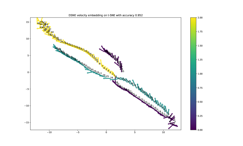
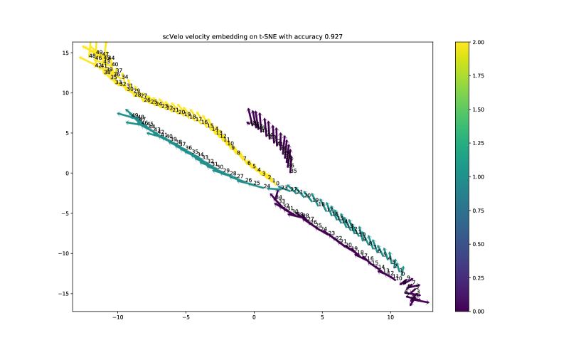
Figure 1: The toy example on the simulated data based on exact data points and velocities with $N=150$, $D=30$. The top figure shows the results of DSNE on the t-SNE map points, which has the accuracy $0.952$ of velocity embeddings compared with the approximate true direction on the t-SNE map points. The bottom figure shows the results of scVeloEmbedding on the t-SNE map points, which has the accuracy $0.927$ of velocity embeddings compared with the approximate true direction on the t-SNE map points.

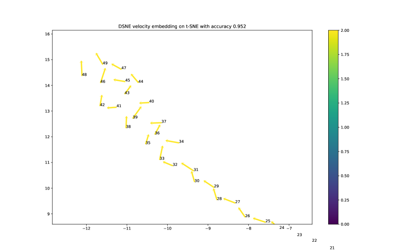
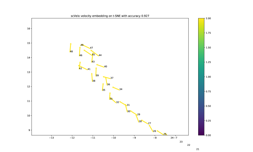
Figure 2: The enlarged plot of top left part of Figure 1

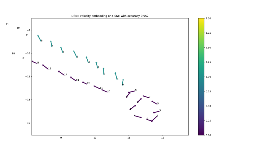
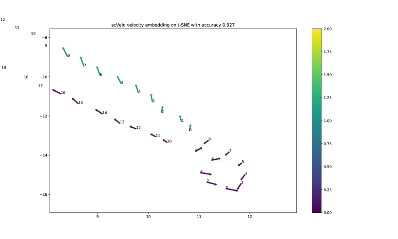
Figure 3: The enlarged plot of bottom right part of Figure 1

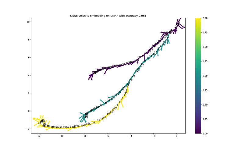
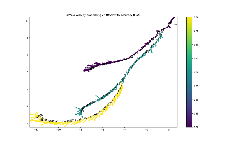
Figure 4: The toy example on the simulated data based on exact data points and velocities with $N=150$, $D=30$. The top figure shows the results of DSNE on the UMAP map points, which has the accuracy $0.961$ of velocity embeddings compared with the approximate true direction on the UMAP map points. The bottom figure shows the results of scVeloEmbedding on the UMAP map points, which has the accuracy $0.927$ of velocity embeddings direction compared with the approximate true direction on the UMAP map points. Zoom in for details.

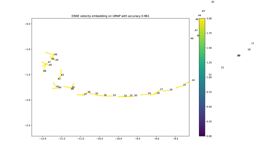
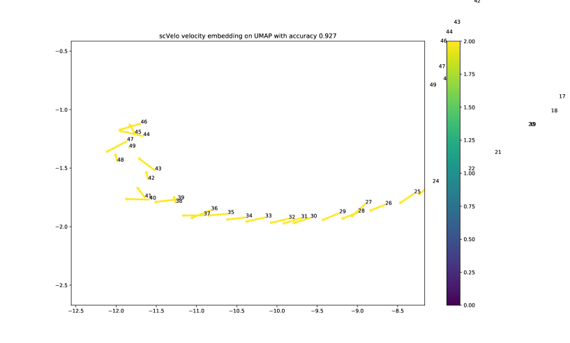
Figure 5: The enlarged plot of top left part of Figure 4

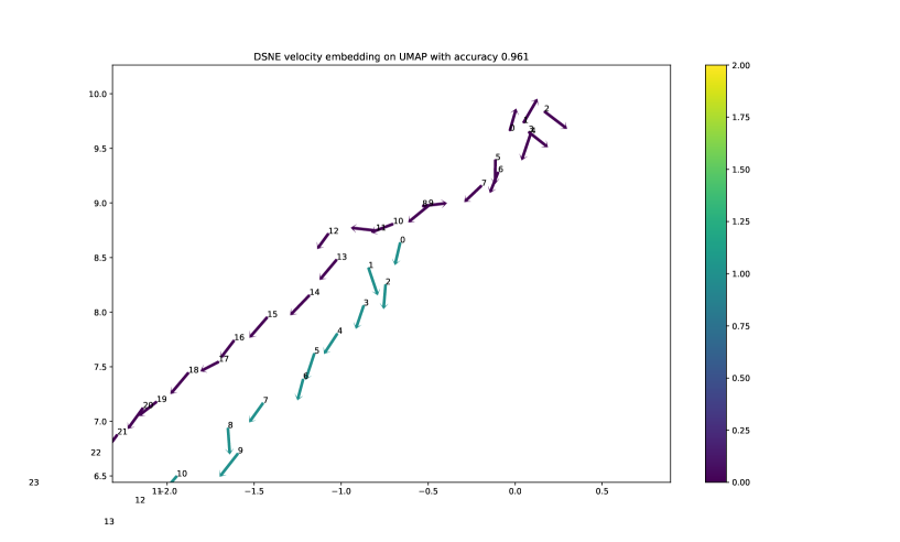
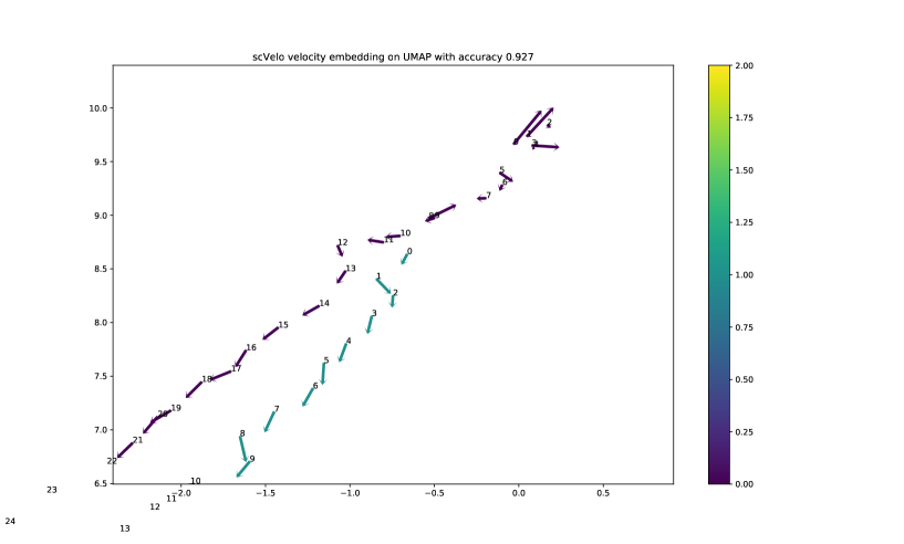
Figure 6: The enlarged plot of bottom right part of Figure 4

To more throughly test the performance of DSNE and compare with the scVeloEmbedding, we simulate the data $10$ times with different dimensions of $N,D$, and compute the low-dimension map points with BH-SNE (van der Maaten, (2013)) (https://github.com/danielfrg/tsne) with parameter $\theta=0.5,\;Perplexity=20$, UMAP (Mcinnes and Healy, (2018)), run DSNE and scVeloEmbedding on the same simulated data with same map points each time. For DSNE, we use $K=6,\;perplexity=1$ on the setting $N=150,\;D=30$ and $K=16,\;perplexity=3$ for all other settings. For scVeloEmbedding, we run it with the default parameter in the scVelo (https://github.com/theislab/scvelo) package. Finally, we output the mean and standard deviation of the accuracy in Table 1. From the table, we see that DSNE do a better work than scVeloEmbedding for all the test settings.

Table 1: Accuracy of Direction of Velocity Embeddins on the Simulation Data with Approximate Map Points and Velocity Embeddings

Dimension (Reduction Method)	Accuracy mean (std) of DSNE	Accuracy mean (std) of scVeloEmbedding
$N=150,\;D=30$  ( UMAP)	$0.965~{}(0.007)$	$0.936~{}(0.011)$
$N=150,\;D=30$   ( t-SNE )	$0.959~{}(0.006)$	$0.925~{}(0.004)$
$N=1500,\;D=10$  ( UMAP)	$0.985~{}(0.002)$	$0.944~{}(0.009)$
$N=1500,\;D=10$   ( t-SNE )	$0.982~{}(0.003)$	$0.936~{}(0.001)$
$N=1500,\;D=300$ ( UMAP)	$0.988~{}(0.002)$	$0.969~{}(0.003)$
$N=1500,\;D=300$   ( t-SNE )	$0.985~{}(0.002)$	$0.961~{}(0.002)$
$N=15000,\;D=300$  ( UMAP )	$0.988~{}(0.001)$	$0.969~{}(0.001)$
$N=15000,\;D=300$   ( t-SNE )	$0.993~{}(0.001)$	$0.981~{}(0.001)$

To get a visual feeling on the velocity embeddings, we plot the stream, grid, arrow plot of the results of DSNE and scVeloEmbedding on the UMAP map points ( see Figure 7, Figure 8, Figure 9) and on the t-SNE map points ( see Figure 10, Figure 11, Figure 12). From the UMAP stream plot (Figure 7), we see that DSNE present a well stream line along the map points. while scVeloEmbedding present over-smoothed stream lines along the map points. Also we note that UMAP is a better representation of the global structure than t-SNE map points, since each color line is a swig line in the high dimension space, t-SNE map points break the line into small pieces in the low-dimensional space, while UMAP keeps the continuous line for each color.

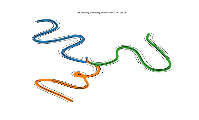
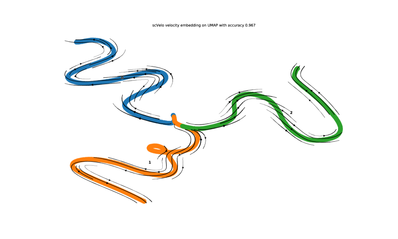
Figure 7: The stream plot of the simulated data based on exact data points and velocities with $N=1500$, $D=300$ and $d=2$. The top figure shows the stream plot of the velocity embeddings output by DSNE on the UMAP map points of the data points, which has the direction accuracy $0.987$ compared with the approximate true velocity embeddings; the bottom figure shows the stream plot of the velocity embeddings output by scVeloEmbeddings on the UMAP map points of the data points, which has the direction accuracy $0.967$. Zoom in for details.

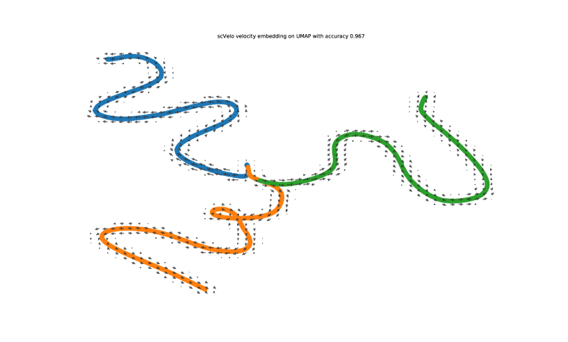
Figure 8: The grid plot of the simulated data based on exact data points and velocities with $N=1500$, $D=300$ and $d=2$. The top figure shows the grid plot of the velocity embeddings output by DSNE on the UMAP map points of the data points, which has the direction accuracy $0.987$ compared with the approximate true velocity embeddings; the bottom figure shows the grid plot of the velocity embeddings output by scVeloEmbeddings on the UMAP map points of the data points, which has the direction accuracy $0.967$. Zoom in for details.

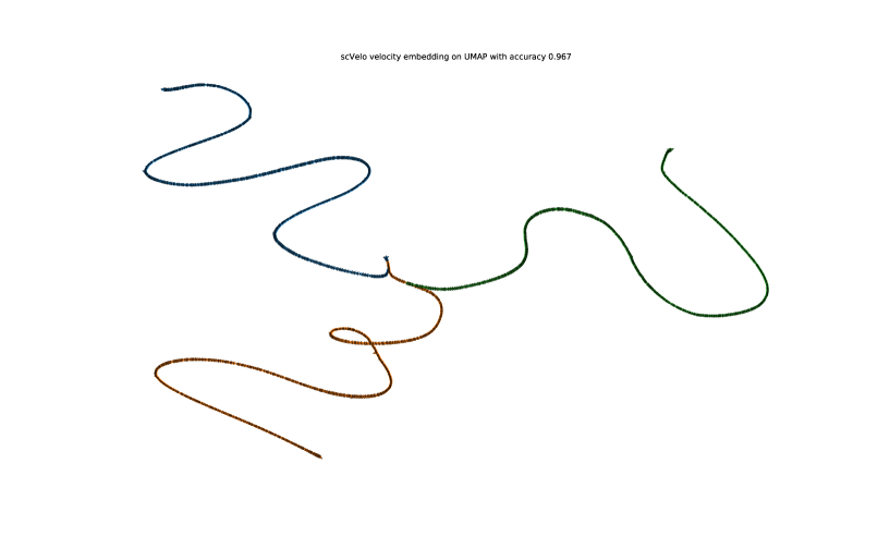
Figure 9: The arrow plot of the simulated data based on exact data points and velocities with $N=1500$, $D=300$ and $d=2$. The top figure shows the arrow plot of the velocity embeddings output by DSNE on the UMAP map points of the data points, which has the direction accuracy $0.987$ compared with the approximate true velocity embeddings; the bottom figure shows the arrow plot of the velocity embeddings output by scVeloEmbeddings on the UMAP map points of the data points, which has the direction accuracy $0.967$. Zoom in for details.

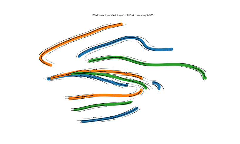
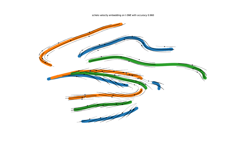
Figure 10: The stream plot of the simulated data based on exact data points and velocities with $N=1500$, $D=300$ and $d=2$. The top figure shows the stream plot of the velocity embeddings output by DSNE on the t-SNE map points of the data points, which has the direction accuracy $0.983$ compared with the approximate true velocity embeddings; the bottom figure shows the stream plot of the velocity embeddings output by scVeloEmbeddings on the t-SNE map points of the data points, which has the direction accuracy $0.960$. Zoom in for details.

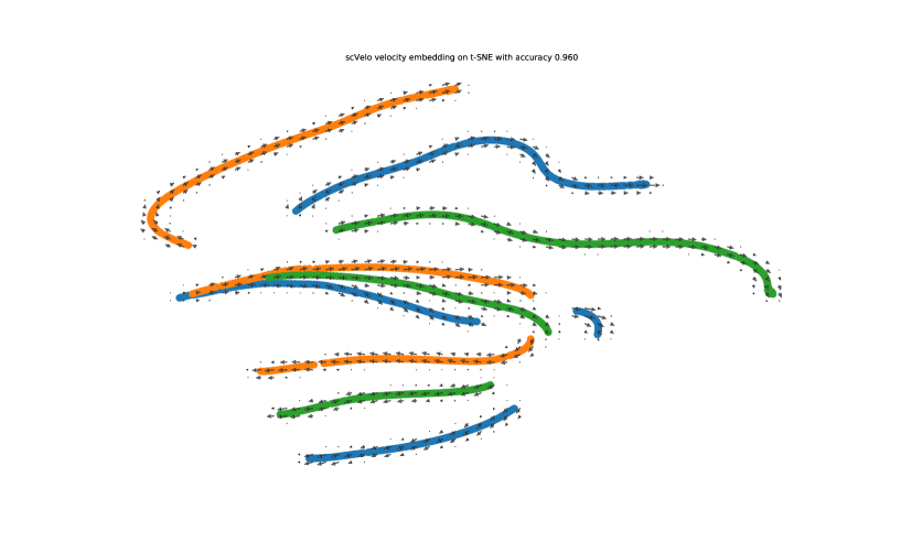
Figure 11: The grid plot of the simulated data based on exact data points and velocities with $N=1500$, $D=300$ and $d=2$. The top figure shows the grid plot of the velocity embeddings output by DSNE on the t-SNE map points of the data points, which has the direction accuracy $0.983$ compared with the approximate true velocity embeddings; the bottom figure shows the grid plot of the velocity embeddings output by scVeloEmbeddings on the t-SNE map points of the data points, which has the direction accuracy $0.960$. Zoom in for details.

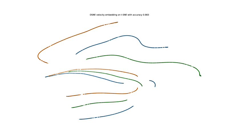
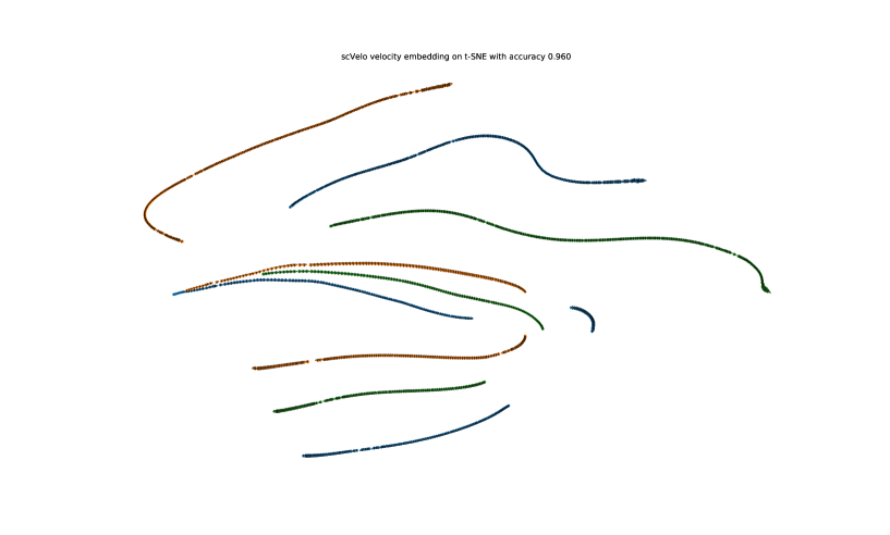
Figure 12: The arrow plot of the simulated data based on exact data points and velocities with $N=1500$, $D=300$ and $d=2$. The top figure shows the arrow plot of the velocity embeddings output by DSNE on the t-SNE map points of the data points, which has the direction accuracy $0.983$ compared with the approximate true velocity embeddings; the bottom figure shows the arrow plot of the velocity embeddings output by scVeloEmbeddings on the t-SNE map points of the data points, which has the direction accuracy $0.960$. Zoom in for details.

5.1.2 Simulation with known low dimensional velocity

To get the exact quantitive measure how the DSNE and scVeloEmbedding behave, we generate the simulation data which begin with velocity embeddings on the low dimensional space, and then moving along the velocity embedding with one time step one-by-one from three start points to get the map points. Then we linear project the map points and their velocities to the high dimensional space. By this way, we have the true velocity embeddings and map points of the corresponding high dimensional data points and velocities. We compare the velocity embeddings $W$ with the true velocity embeddings $W_{true}$ by the cosine distances, i.e, we define the accuracy of velocity embeddings $W$ with the true velocity embeddings $W_{true}$ by

$$accu:=\frac{1}{N}\sum\langle\frac{w_{i}}{||w_{i}||},\frac{w_{true,i}}{||w_{true,i}||}\rangle$$ (27)

where $accu\in[-1,1]$, the perfect accuracy is $1$ with all the velocity embeddings direction correct, $\frac{w_{i}}{||w_{i}||}=\frac{w_{true,i}}{||w_{true,i}},\;i=1,\ldots,N$; the lowest accuracy is $-1$ with all the velocity embeddings direction are the opposite of the true velocity embeddings direction, $\frac{w_{i}}{||w_{i}||}=-\frac{w_{true,i}}{||w_{true,i}||},\;i=1,\ldots,N$.

The simulate data was generated similarly as above.

1. Generate the low-dimensional velocity $W_{true}\in\mathbb{R}^{N\times D}$ by random sampling from the Normal distributions, $W_{true,il}\sim\mathcal{N}(0,36),\;i=1\ldots,N;\;l=1,\ldots,d$. where we take $N=3N_{s}$;

2. Choose there start points of map points $y_{start,1}=\mathbf{0}$, $y_{start,2}=50*\mathbf{1}$. $y_{start,3}=160*\mathbf{1}$. where $\mathbf{0}$ is the zeros vector with length $d$ and $\mathbf{1}$ is the ones vector with length $d$.

3. Generate the map points by moving from the three starting points along with the velocity embedding $w_{i}$ one by one, i.e.

   $$\begin{array}[]{l}y_{1}=y_{start,1}\\ y_{N_{s}+1}=y_{start,2}\\ y_{2N_{s}+1}=y_{start,3}\\ y_{i+1}=y_{i}+w_{true,i},\;i=1,\ldots,N_{s}-1\\ y_{N_{s}+i+1}=y_{N_{s}+i}+w_{true,i},\;i=1,\ldots,N_{s}-1\\ y_{2N_{s}+i+1}=y_{2N_{s}+i}+w_{true,i},\;i=1,\ldots,N_{s}-1\\ \end{array}$$

4. Generate the projection matrix $U\in\mathbb{R}^{d\times D}$ by random sampling from the standard normal distributions, i.e. $U_{kl}\sim\mathcal{N}(0,1),\;k=1,\ldots,d;\;l=1,\ldots,D$.

5. Projection the map points $Y$ and the true velocity embeddings $W_{true}$ by the projection matrix $U$ to get the data points $X=YU$ and velocity matrix $V=W_{true}U$.

We run the DSNE and scVeloEmbedding to learn the velocity embeddings and finally compare the accuracy defined in equation (27) to see how good the two algorithms behave. To compare the performance, we run simulation data with same $N,D$ $10$ times, run the DSNE and scveloEmbedding algorithm on the same simulated data each time. For DSNE, we select the parameter $K=16$, $perplexity=6$ for all settings. We run scVeloEmbedding with default parameters in scVelo package ($K=100$). The mean with the standard deviation of the accuracies of the $10$ times for different $N$ and $D$ are presented in Table 2. It obviously that DSNE do a better work than scVeloEmbedding on all the test settings.

Table 2: Accuracy of Direction of Velocity Embedding on the Simulation Data with Exact Map Points and Velocity Embeddings

Name	Accuracy mean (std) of DSNE	Accuracy mean (std) of scVeloEmbedding
$N=150,\;D=30$	$0.980~{}(0.011)$	$0.914~{}(0.010)$
$N=1500,\;D=10$	$0.985~{}(0.007)$	$0.965~{}(0.003)$
$N=1500,\;D=300$	$0.994~{}(0.002)$	$0.966~{}(0.007)$
$N=15000,\;D=300$	$0.995~{}(0.001)$	$0.983~{}(0.003)$

To get a feel about the velocity embedding, we plot the stream, grid, arrow picture in Figure 13, Figure 14, Figure 15, respectively. From the arrow picture ( Figure 15 ), we found that arrow length of DSNE was better presented than scVeloEmbedding’s, this verifies the effectiveness of the approximate formula (20).

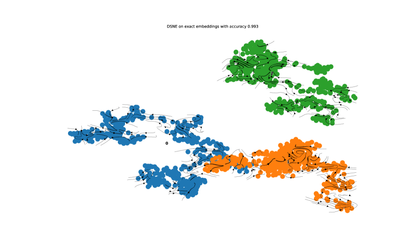
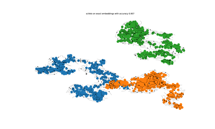
Figure 13: The stream plot of the simulated data based on exact map points and velocity embeddings with $N=1500$, $D=300$ and $d=2$. The top figure shows the stream plot of the velocity embeddings output by DSNE, which has the direction accuracy $0.993$ compared with the true velocity embeddings; the bottom figure shows the stream plot of the velocity embeddings output by scVeloEmbedding, which has the direction accuracy $0.957$. Zoom in for details.

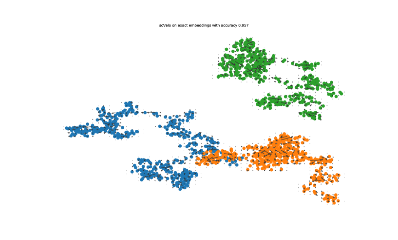
Figure 14: The grid plot of the simulated data based on exact map points and velocity embeddings with $N=1500$, $D=300$ and $d=2$. The top figure shows the stream plot of the velocity embeddings output by DSNE, which has the direction accuracy $0.993$ compared with the true velocity embeddings; the bottom figure shows the stream plot of the velocity embeddings output by scVeloEmbeddings, which has the direction accuracy $0.957$. Zoom in for details.

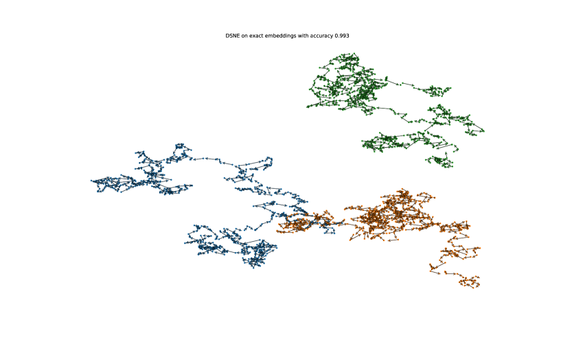
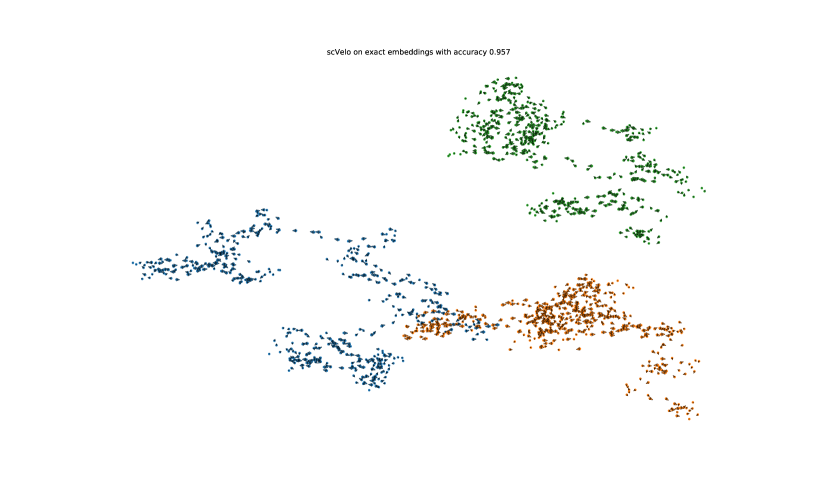
Figure 15: The arrow plot of the simulated data based on exact map points and velocity embeddings with $N=1500$, $D=300$ and $d=2$. The top figure shows the stream plot of the velocity embeddings output by DSNE, which has the direction accuracy $0.993$ compared with the true velocity embeddings; the bottom figure shows the stream plot of the velocity embeddings output by scVeloEmbeddings, which has the direction accuracy $0.957$. Zoom in for details.

5.2 scRNA-seq data: Endocrine Pancreas

The cell differentiation and embryo development is the fundamental problems in biology. RNA velocity techniques greatly aid to make a visually view how the cell trajectory presented on the low dimensional space. Here, we use the Pancreas data which was analyzed in Bergen et al., (2020) to compare DSNE with the scVeloEmbedding.

We run DSNE with parameters $K=16$, $perplexity=3$ and run scVeloEmbedding with the default parameters, which is based on the notebooks from https://github.com/theislab/scvelo_notebooks/Pancreas.ipynb. For the low dimensional map points, we use the UMAP map points and VeloViz(Atta and Fan, (2021)) map points which was based the tutorial https://github.com/JEFworks-Lab/veloviz/vignettes/pancreas.Rmd.

We plot the stream, grid, arrow plot in Fig 16, Fig 17, Fig 18 for UMAP map points, respectively; and Fig 19, Fig 20, Fig 21 for VeloViz map points, respectively.

On the UMAP stream plot (Fig 16) and grid plot ( Fig 17), we found that scVeloEmbedding seems over smooth the velocity direction to the mean direction, while DSNE reveal more details for the local moving trend on the map, which may helpful to identify some special cells in the data. For the VeloViz Plots, it occurs the similar phenomenon. Note that the VeloViz organize cell clusters on the map were different from the UMAP, and which is better representation need to be checked by the biologists.

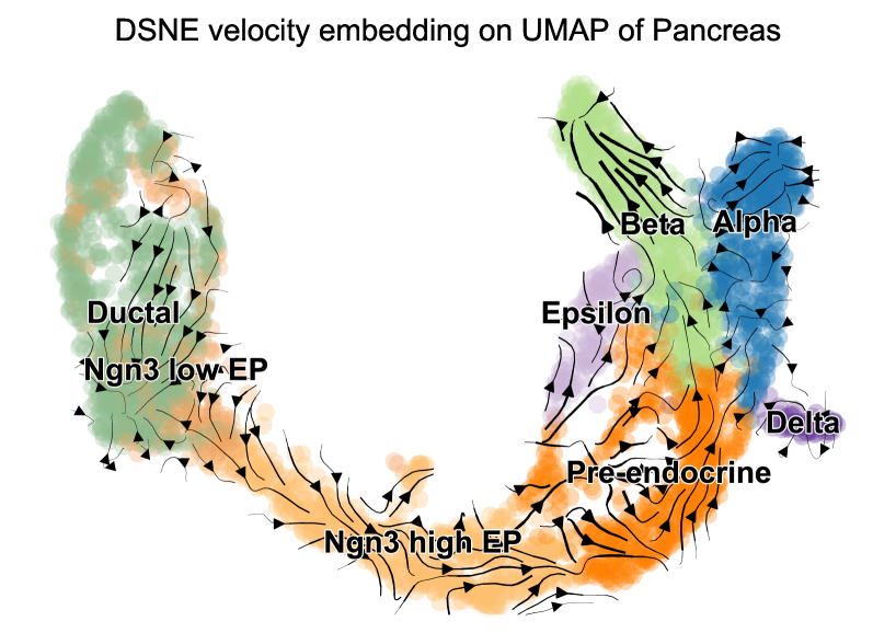
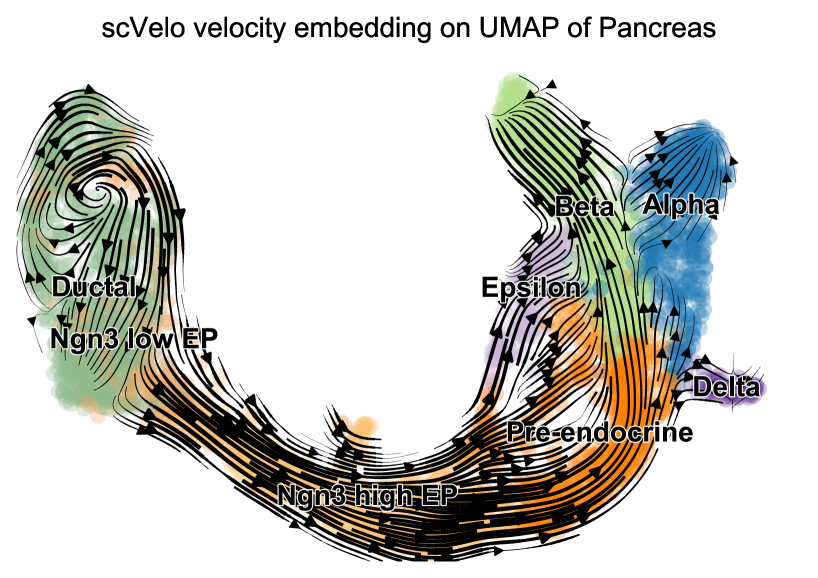
Figure 16: The stream plot of the velocity embeddings on the UMAP of the pancreas data. The top figure shows the results of DSNE and the bottom figure shows the results of scVeloEmbedding. Zoom in for details.

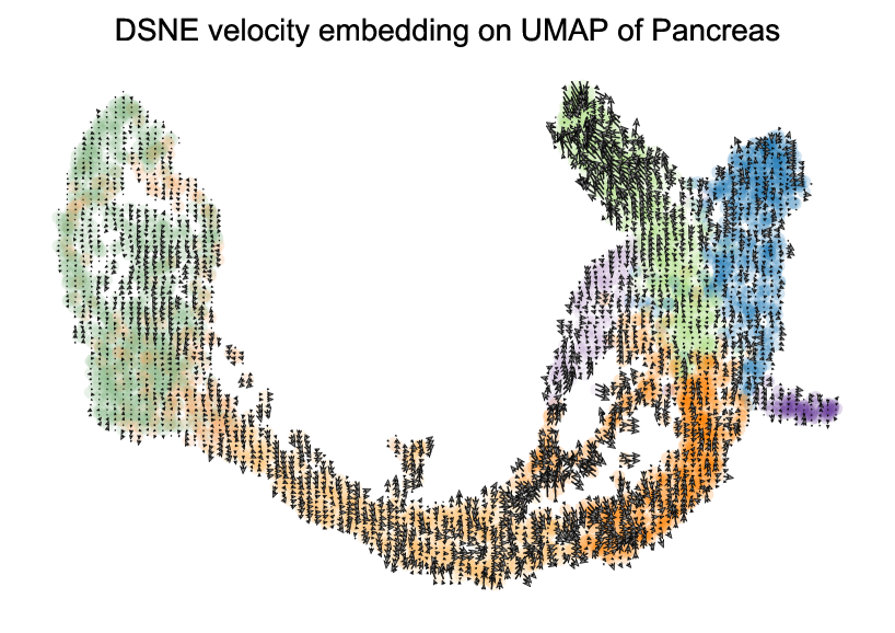
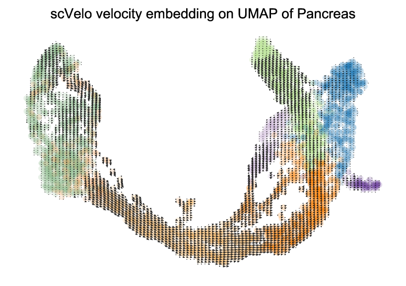
Figure 17: The grid plot of the velocity embeddings on the UMAP of the pancreas data. The top figure shows the results of DSNE and the bottom figure shows the results of scVeloEmbedding. Zoom in for details.

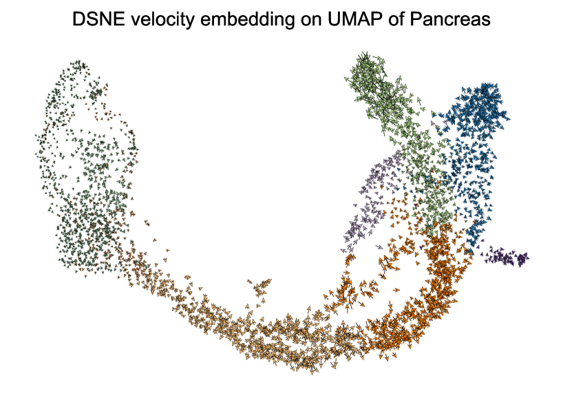
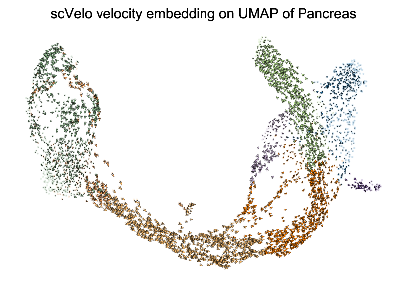
Figure 18: The arrow plot of the velocity embeddings on the UMAP of the pancreas data. The top figure shows the results of DSNE and the bottom figure shows the results of scVeloEmbedding. Zoom in for details.

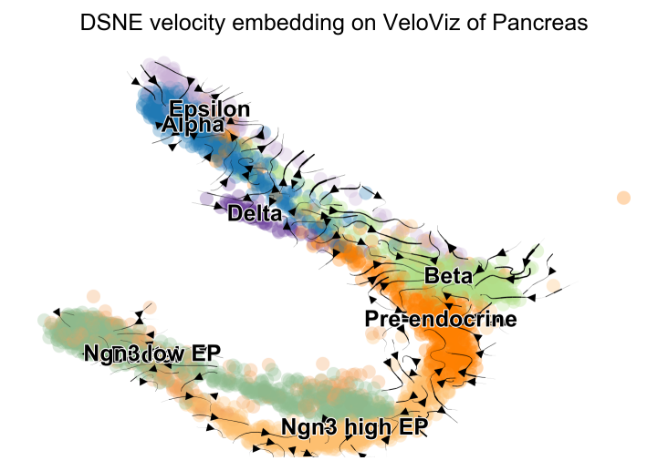
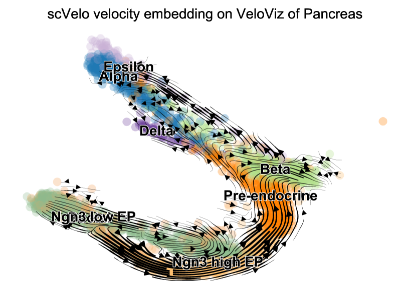
Figure 19: The stream plot of the velocity embeddings on the VeloViz map points of the pancreas data. The top figure shows the results of DSNE and the bottom figure shows the results of scVeloEmbedding. Zoom in for details.

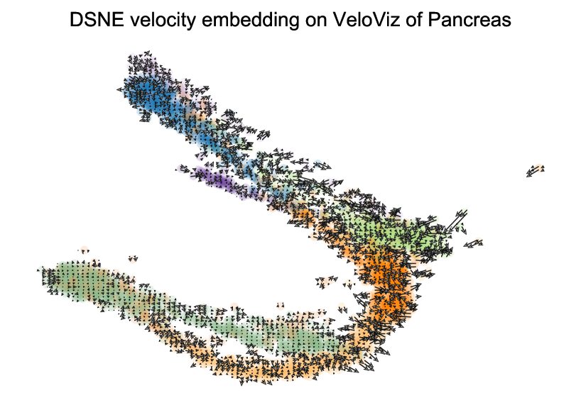
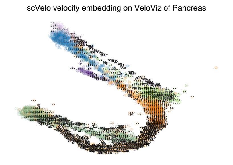
Figure 20: The grid plot of the velocity embeddings on the VeloViz map points of the pancreas data. The top figure shows the results of DSNE and the bottom figure shows the results of scVeloEmbedding. Zoom in for details.

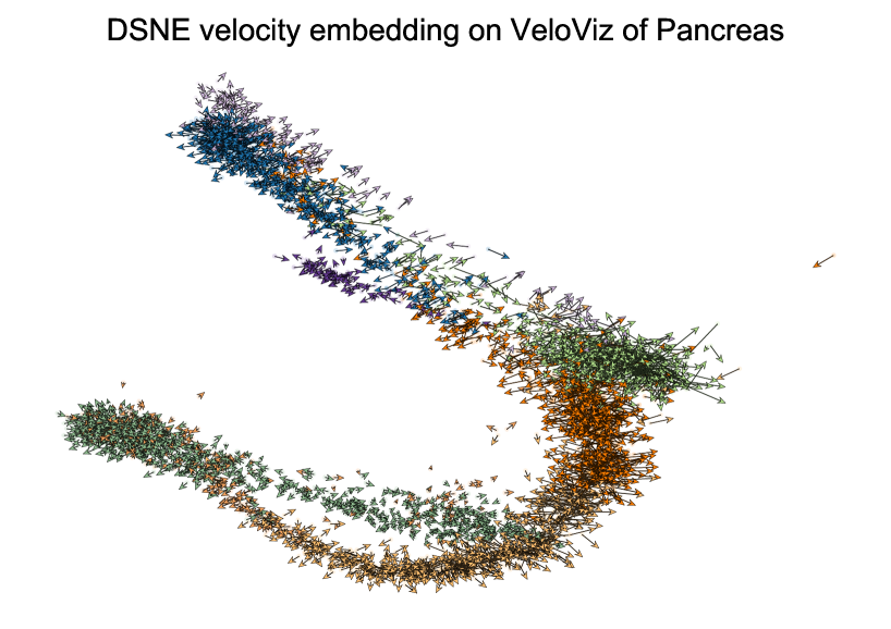
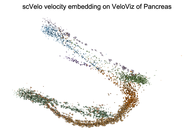
Figure 21: The arrow plot of the velocity embeddings on the VeloViz map points of the pancreas data. The top figure shows the results of DSNE and the bottom figure shows the results of scVeloEmbedding. Zoom in for details.

6 Discussion

Currently, we leaning the embedding of the velocity with known low-dimensional embedding of map points, it is more reasonable to learn the map points and the velocity embedding of the high dimensional data points and its velocities simultaneously, this need to more dedicate design of methods, since it is hard to adjust the map points and its velocity in the low dimension space to reduce the cost stably, this opens new research opportunity. Atta and Fan, (2021) recently proposed VeloViz method is the effort to that direction, which gets the low dimensional embeddings with the velocity informations comes from the probability distribution which transformed from the distance of points $x_{i}$ with velocity $v_{i}$ and $x_{j}$. It is helpful to organize the low dimensional points which contains the velocity information.

To recovery the velocity embedding on the low dimension map points, it must preserve the local direction information in the low dimensional space, e.g. $||\hat{v}_{i}-\Delta\hat{x}_{ij}||^{2}=\alpha||\hat{w}_{i}-\Delta\hat{y}_{ij}||^{2},\;j\in\text{i's neighbors}$ for some positive scalar $\alpha$. This is not specially emphasized in the dimension reduction techniques, e.g., t-SNE, UMAP, which left to the future work.

7 Conclusion

In this paper, we propose DSNE to get the low dimensional velocity embeddings when given the high dimensional data points with its velocities and the low dimensional map points. The numerical experiments show that DSNE can faithfully keep the direction of the velocity in the low dimensional space correspond to the velocity direction in the high dimensional space. It is helpful to visualize the cell trajectories in the biological science, which may aid to check how the cells move around its near neighbors, and the global structures may give us the sense the development relations of different cell subtypes. We hope that this method can help to recovery mystery of the cell differentiation and embryo development. And we also expect that you can find more usages of this method.

Appendix A. Code availability

DSNE are available as python package on https://github.com/songtingstone/dsne. Scripts to reproduce results of the primary analyses will be made available on  https://github.com/songtingstone/dsne2021. The code is learned and adapted the C implementation https://github.com/danielfrg/tsne of BH-SNE (van der Maaten, (2013)), special thanks to Laurens van der Maaten and Daniel Rodriguez.

Appendix B. Derivation of the DSNE gradient and Hessian matrix.

DSNE use the scaled KL divergence as the loss function

$$\begin{array}[]{l}C=\sum_{i}\sum_{j\in\text{i's neighbors}}\tilde{p}_{j|i}\log\frac{p_{j|i}}{q_{j|i}}\end{array}$$ (28)

where

$$\begin{array}[]{l}p_{j|i}=\frac{1}{Z_{x,i}}\exp(-2\beta_{x,i}(1-\cos_{x,ij})),\;j\in\text{ i's neighbors }\\ p_{i|i}=\frac{1}{Z_{x,i}}\\ Z_{x,i}=1+\sum_{j\in\text{ i's neighbors }}\exp(-2\beta_{x,i}(1-\cos_{x,ij}))\\ \cos_{x,ij}=\langle\hat{v}_{i},\Delta\hat{x}_{ij}\rangle\\ \tilde{p}_{j|i}=\frac{1}{\tilde{Z}_{x,i}}\exp(-2\beta_{x,i}(1-\cos_{x,ij})),\;j\in\text{ i's neighbors }\\ \tilde{p}_{i|i}=0\\ \tilde{Z}_{x,i}=\sum_{j\in\text{ i's neighbors }}\exp(-2\beta_{x,i}(1-\cos_{x,ij}))\\ q_{j|i}=\frac{1}{Z_{y,i}}\exp(-2\beta_{y,i}(1-\cos_{y,ij}))\;j\in\text{ i's neighbors }\\ q_{i|i}=\frac{1}{Z_{y,i}}\\ Z_{y,i}=1+\sum_{j\in\text{ i's neighbors }}\exp(-2\beta_{y,i}(1-\cos_{y,ij}))\\ \cos_{y,ij}=\langle\hat{w}_{i},\Delta\hat{y}_{ij}\rangle\\ \hat{w}_{i}=\frac{w}{||w||}\\ \end{array}$$ (29)

Note that $w_{i},\beta_{y,i}$ are independent of each other, so that we can separate the loss into part of $i$,

$$\begin{array}[]{l}C=\sum_{i}C_{i}\\ C_{i}=\sum_{j\in\text{i's neighbors}}\tilde{p}_{j|i}\log\frac{p_{j|i}}{q_{j|i}}\end{array}$$ (30)

To simplify the notation, we define $\hat{q}_{j|i}:=\exp(-2\beta_{y,i}(1-\cos_{y,ij}))$, so that $Z_{y,i}=1+\sum_{j\in\text{ i's neighbors }}\hat{q}_{j|i}$ and $q_{j|i}=\frac{\hat{q}_{j|i}}{Z_{y,i}}$.

The gradient of the cost function $C$ with respect to $w_{i}$ is given by

$$\begin{array}[]{ll}\frac{\partial C}{\partial w_{i}}&=\frac{\partial C_{i}}{\partial w_{i}}\\ &=\frac{\partial}{\partial w_{i}}[\sum_{j\in\text{i's neighbors}}\tilde{p}_{j|i}\log\frac{p_{j|i}}{q_{j|i}}]\\ &=\frac{\partial}{\partial w_{i}}[\sum_{j\in\text{i's neighbors}}-\tilde{p}_{j|i}\log q_{j|i}]\\ &=-\sum_{j\in\text{i's neighbors}}-\tilde{p}_{j|i}\frac{\partial}{\partial w_{i}}[\log q_{j|i}]\\ &=-\sum_{j\in\text{i's neighbors}}\tilde{p}_{j|i}\frac{\partial}{\partial w_{i}}[\log\hat{q}_{j|i}-\log Z_{y,i}]\\ &=-\sum_{j\in\text{i's neighbors}}\tilde{p}_{j|i}\frac{\partial}{\partial w_{i}}[\log\hat{q}_{j|i}]+\frac{\partial}{\partial w_{i}}\log Z_{y,i}\\ &=-\sum_{j\in\text{i's neighbors}}\tilde{p}_{j|i}\frac{\partial}{\partial w_{i}}[\log\hat{q}_{j|i}]+\frac{1}{Z_{y,i}}\frac{\partial}{\partial w_{i}}Z_{y,i}\\ &=-\sum_{j\in\text{i's neighbors}}\tilde{p}_{j|i}\frac{\partial}{\partial w_{i}}[\log\hat{q}_{j|i}]+\frac{1}{Z_{y,i}}\frac{\partial}{\partial w_{i}}[1+\sum_{j\in\text{ i's neighbors }}\hat{q}_{j|i}]\\ &=-\sum_{j\in\text{i's neighbors}}\tilde{p}_{j|i}\frac{\partial}{\partial w_{i}}[\log\hat{q}_{j|i}]+\frac{1}{Z_{y,i}}\sum_{j\in\text{ i's neighbors }}\hat{q}_{j|i}\frac{\partial}{\partial w_{i}}[\log\hat{q}_{j|i}]\\ &=-\sum_{j\in\text{i's neighbors}}\tilde{p}_{j|i}\frac{\partial}{\partial w_{i}}[\log\hat{q}_{j|i}]+\sum_{j\in\text{ i's neighbors }}q_{j|i}\frac{\partial}{\partial w_{i}}[\log\hat{q}_{j|i}]\\ &=-\sum_{j\in\text{i's neighbors}}(\tilde{p}_{j|i}-q_{j|i})\frac{\partial}{\partial w_{i}}[\log\hat{q}_{j|i}]\end{array}$$ (31)

where the sixth equality comes from the fact $\sum_{j\in\text{i's neighbors}}\tilde{p}_{j|i}=1$. Note that

$$\begin{array}[]{ll}\frac{\partial}{\partial w_{i}}[\log\hat{q}_{j|i}]&=\frac{\partial}{\partial w_{i}}[-2\beta_{y,i}(1-\cos_{y,ij})]\\ &=2\beta_{y,i}\frac{\partial}{\partial w_{i}}[\cos_{y,ij}]\\ &=2\beta_{y,i}\frac{\partial}{\partial w_{i}}\langle\frac{w_{i}}{||w_{i}||},\Delta\hat{y}_{ij}\rangle\\ &=2\beta_{y,i}[\frac{\Delta\hat{y}_{ij}}{||w_{i}||}-\langle w_{i},\Delta\hat{y}_{ij}\rangle\frac{w_{i}}{||w_{i}||^{3}}]\\ &=\frac{2\beta_{y,i}}{||w_{i}||}(\Delta\hat{y}_{ij}-cos_{y,ij}\hat{w}_{i})\end{array}$$ (32)

The gradient of the cost function $C$ with respect to $w_{i}$ is given by

$$\begin{array}[]{ll}\frac{\partial C}{\partial w_{i}}&=-\sum_{j\in\text{i's neighbors}}(\tilde{p}_{j|i}-q_{j|i})\frac{\partial}{\partial w_{i}}[\log\hat{q}_{j|i}]\\ &=-\sum_{j\in\text{i's neighbors}}(\tilde{p}_{j|i}-q_{j|i})\frac{2\beta_{y,i}}{||w_{i}||}(\Delta\hat{y}_{ij}-cos_{y,ij}\hat{w}_{i})\\ &=\sum_{j\in\text{i's neighbors}}(\tilde{p}_{j|i}-q_{j|i})\frac{2\beta_{y,i}}{||w_{i}||}(-\Delta\hat{y}_{ij}+cos_{y,ij}\hat{w}_{i})\end{array}$$ (33)

Similarly, the gradient of the cost function $C$ with respect to $\beta_{y,i}$ is given by

$$\begin{array}[]{ll}\frac{\partial C}{\partial\beta_{y,i}}&=-\sum_{j\in\text{i's neighbors}}(\tilde{p}_{j|i}-q_{j|i})\frac{\partial}{\partial\beta_{y,i}}[\log\hat{q}_{j|i}]\\ &=-\sum_{j\in\text{i's neighbors}}(\tilde{p}_{j|i}-q_{j|i})[-2(1-\cos_{y,ij})]\\ &=\sum_{j\in\text{i's neighbors}}(\tilde{p}_{j|i}-q_{j|i})2(1-\cos_{y,ij})\end{array}$$ (34)

Next we derive the second order gradient of the DSNE cost function. It basically use the same trick as in equation(31), but with a little more complex calculations.

For the second order gradient of the cost function with respect to $w_{i}$, we calculate $\frac{\partial}{\partial w_{i}}[\frac{\partial C}{\partial w_{i}}(1)]$ first, where we use $x(1)$ to denote the first element of vector $x$. Note that $\frac{\partial C}{\partial w_{i}}(1)=\sum_{j\in\text{i's neighbors}}(\tilde{p}_{j|i}-q_{j|i})\frac{2\beta_{y,i}}{||w_{i}||}(-\Delta\hat{y}_{ij}(1)+cos_{y,ij}\hat{w}_{i}(1))$. So we have

$$\begin{array}[]{ll}\frac{\partial}{\partial w_{i}}[\frac{\partial C}{\partial w_{i}}(1)]&=\frac{\partial}{\partial w_{i}}[\sum_{j\in\text{i's neighbors}}(\tilde{p}_{j|i}-q_{j|i})\frac{2\beta_{y,i}}{||w_{i}||}(-\Delta\hat{y}_{ij}(1)+cos_{y,ij}\hat{w}_{i}(1))]\\ &=\frac{\partial}{\partial w_{i}}[\sum_{j\in\text{i's neighbors}}(\tilde{p}_{j|i}-q_{j|i})\frac{2\beta_{y,i}}{||w_{i}||}(-\Delta\hat{y}_{ij}(1)+cos_{y,ij}\hat{w}_{i}(1))]\\ &=\frac{\partial}{\partial w_{i}}[\sum_{j\in\text{i's neighbors}}(\tilde{p}_{j|i}-q_{j|i})2\beta_{y,i}(-\frac{\Delta\hat{y}_{ij}(1)}{||w_{i}||}+\langle w_{i},\Delta\hat{y}_{ij}\rangle\frac{w_{i}(1)}{||w_{i}||^{3}})]\\ &=\sum_{j\in\text{i's neighbors}}(\tilde{p}_{j|i}-q_{j|i})2\beta_{y,i}\frac{\partial}{\partial w_{i}}[-\frac{\Delta\hat{y}_{ij}(1)}{||w_{i}||}+\langle w_{i},\Delta\hat{y}_{ij}\rangle\frac{w_{i}(1)}{||w_{i}||^{3}}]\\ &\quad-\sum_{j\in\text{i's neighbors}}2\beta_{y,i}(-\frac{\Delta\hat{y}_{ij}(1)}{||w_{i}||}+\langle w_{i},\Delta\hat{y}_{ij}\rangle\frac{w_{i}(1)}{||w_{i}||^{3}})\frac{\partial}{\partial w_{i}}[q_{j|i}]\\ \end{array}$$ (35)

$$\begin{array}[]{ll}&\quad\frac{\partial}{\partial w_{i}}[-\frac{\Delta\hat{y}_{ij}(1)}{||w_{i}||}+\langle w_{i},\Delta\hat{y}_{ij}\rangle\frac{w_{i}(1)}{||w_{i}||^{3}}]\\ &=\Delta\hat{y}_{ij}(1)\frac{w_{i}}{||w_{i}||^{3}}+\Delta\hat{y}_{ij}\frac{w_{i}(1)}{||w_{i}||^{3}}+\langle w_{i},\Delta\hat{y}_{ij}\rangle\frac{1}{||w_{i}||^{3}}e_{1}-3\langle w_{i},\Delta\hat{y}_{ij}\rangle w_{i}(1)\frac{w_{i}}{||w_{i}||^{5}}\\ &=\frac{1}{||w_{i}||^{2}}(\Delta\hat{y}_{ij}(1)\hat{w}_{i}+\Delta\hat{y}_{ij}\hat{w}_{i}(1)+cos_{y,ij}e_{1}-3cos_{y,ij}\hat{w}_{i}(1)\hat{w}_{i})\end{array}$$ (36)

where $e_{1}=[1,0,\ldots,0]\in\mathbb{R}^{d}$.

$$\begin{array}[]{ll}\frac{\partial}{\partial w_{i}}q_{j|i}&=\frac{\partial}{\partial w_{i}}[\frac{\hat{q}_{j|i}}{Z_{y,i}}]\\ &=Z_{y,i}^{-1}\frac{\partial}{\partial w_{i}}[\hat{q}_{j|i}]-\hat{q}_{j|i}Z_{y,i}^{-2}\frac{\partial}{\partial w_{i}}Z_{y,i}\\ &=q_{j|i}\frac{\partial}{\partial w_{i}}[\log\hat{q}_{j|i}]-q_{j|i}\sum_{k\in\text{i's neighbors}}q_{k|i}\frac{\partial}{\partial w_{i}}[\log\hat{q}_{k|i}]\\ &=q_{j|i}\frac{2\beta_{y,i}}{||w_{i}||}(\Delta\hat{y}_{ij}-cos_{y,ij}\hat{w}_{i})-q_{j|i}\sum_{k\in\text{i's neighbors}}q_{k|i}\frac{2\beta_{y,i}}{||w_{i}||}(\Delta\hat{y}_{ik}-cos_{y,ik}\hat{w}_{i})\\ &=q_{j|i}\frac{2\beta_{y,i}}{||w_{i}||}[(\Delta\hat{y}_{ij}-\sum_{k\in\text{i's neighbors}}\Delta\hat{y}_{ik})-\hat{w}_{i}(cos_{y,ij}-\sum_{k\in\text{i's neighbors}}q_{k|i}cos_{y,ik})]\end{array}$$ (37)

Combine equation (35, 36, 37) into one, we get

$$\begin{array}[]{ll}\frac{\partial}{\partial w_{i}}[\frac{\partial C}{\partial w_{i}}(1)]&=\sum_{j\in\text{i's neighbors}}(\tilde{p}_{j|i}-q_{j|i})2\beta_{y,i}\\ &\quad*\frac{1}{||w_{i}||^{2}}(\Delta\hat{y}_{ij}(1)\hat{w}_{i}+\Delta\hat{y}_{ij}\hat{w}_{i}(1)+cos_{y,ij}e_{1}-3cos_{y,ij}\hat{w}_{i}(1)\hat{w}_{i})\\ &\quad-\sum_{j\in\text{i's neighbors}}2\beta_{y,i}(-\frac{\Delta\hat{y}_{ij}(1)}{||w_{i}||}+\langle w_{i},\Delta\hat{y}_{ij}\rangle\frac{w_{i}(1)}{||w_{i}||^{3}})\\ &\quad*q_{j|i}\frac{2\beta_{y,i}}{||w_{i}||}[(\Delta\hat{y}_{ij}-\sum_{k\in\text{i's neighbors}}\Delta\hat{y}_{ik})-\hat{w}_{i}(cos_{y,ij}-\sum_{k\in\text{i's neighbors}}q_{k|i}cos_{y,ik})]\\ \end{array}$$ (38)

From the above equation, it’s easy to see that the second order gradient of cost $C$ with respect to $w_{i}$ is given by

$$\begin{array}[]{ll}\frac{\partial^{2}C}{\partial w_{i}\partial w_{i}^{T}}&=\frac{2\beta_{y,i}}{||w_{i}||^{2}}\sum_{j\in\text{i's neighbors}}(\tilde{p}_{j|i}-q_{j|i})[\Delta\hat{y}_{ij}\hat{w}_{i}^{T}+\hat{w}_{i}\Delta\hat{y}_{ij}^{T}+cos_{y,ij}I-3cos_{y,ij}\hat{w}_{i}\hat{w}_{i}^{T}]\\ &\quad-\frac{4\beta_{y,i}^{2}}{||w||^{2}}\sum_{j\in\text{i's neighbors}}q_{j|i}[-\Delta\hat{y}_{ij}+cos_{y,ij}\hat{w}_{i}][(\Delta\hat{y}_{ij}-\mathbb{E}\Delta\hat{y}_{i})-\hat{w}_{i}(cos_{y,ij}-\mathbb{E}cos_{y,i})]^{T}\\ \end{array}$$ (39)

where $\mathbb{E}\Delta\hat{y}_{i}=\sum_{k\in\text{i's neighbors}}q_{k|i}\Delta\hat{y}_{ik}$, $\mathbb{E}cos_{y,i}=\sum_{k\in\text{i's neighbors}}q_{k|i}\Delta\hat{y}_{ik}$ and $I\in\mathbb{R}^{d\times d}$ is the identity matrix.

Similarly, the second order gradient of cost $C$ with respect to $\beta_{y,i}$ is given by

$$\begin{array}[]{ll}\frac{\partial^{2}C}{\partial^{2}\beta_{y,i}}&=\frac{\partial}{\partial\beta_{y,i}}[\sum_{j\in\text{i's neighbors}}(\tilde{p}_{j|i}-q_{j|i})2(1-\cos_{y,ij})]\\ &=-\sum_{j\in\text{i's neighbors}}2(1-\cos_{y,ij})\frac{\partial}{\partial\beta_{y,i}}q_{j|i}\end{array}$$ (40)

$$\begin{array}[]{ll}\frac{\partial}{\partial\beta_{y,i}}q_{j|i}&=\frac{\partial}{\partial\beta_{y,i}}[\frac{\hat{q}_{j|i}}{Z_{y,i}}]\\ &=Z_{y,i}^{-1}\frac{\partial}{\partial\beta_{y,i}}[\hat{q}_{j|i}]-\hat{q}_{j|i}Z_{y,i}^{-2}\frac{\partial}{\partial\beta_{y,i}}Z_{y,i}\\ &=q_{j|i}\frac{\partial}{\partial\beta_{y,i}}[\log\hat{q}_{j|i}]-q_{j|i}\sum_{k\in\text{i's neighbors}}q_{k|i}\frac{\partial}{\partial\beta_{y,i}}[\log\hat{q}_{k|i}]\\ &=q_{j|i}[-2(1-\cos_{y,ij})]-q_{j|i}\sum_{k\in\text{i's neighbors}}q_{k|i}[-2(1-\cos_{y,ik})]\\ &=-q_{j|i}[2(1-\cos_{y,ij})-\sum_{k\in\text{i's neighbors}}q_{k|i}2(1-\cos_{y,ik})]\end{array}$$ (41)

Combine equation (40, 41) into one, we get the second order gradient of cost $C$ with respect to $\beta_{y,i}$,

$$\begin{array}[]{ll}\frac{\partial^{2}C}{\partial^{2}\beta_{y,i}}&=\sum_{j\in\text{i's neighbors}}2(1-\cos_{y,ij})q_{j|i}[2(1-\cos_{y,ij})-\sum_{k\in\text{i's neighbors}}q_{k|i}2(1-\cos_{y,ik})]\\ &=4[\sum_{j\in\text{i's neighbors}}q_{j|i}(1-\cos_{y,ij})^{2}-(\sum_{j\in\text{i's neighbors}}q_{j|i}(1-\cos_{y,ij}))^{2}]\end{array}$$ (42)

References

• Atta and Fan, (2021) Atta, L. and Fan, J. (2021). VeloViz: RNA-velocity informed 2d embeddings for visualizing cellular trajectories. bioRxiv.
• Bergen et al., (2020) Bergen, V., Lange, M., Peidli, S., Wolf, F. A., and Theis, F. J. (2020). Generalizing RNA velocity to transient cell states through dynamical modeling. Nature Biotechnology, 38(12):1408–1414.
• Hinton and Roweis, (2003) Hinton, G. and Roweis, S. (2003). Stochastic neighbor embedding. Advances in Neural Information Processing Systems, 15(4):833–840.
• Jacobs, (1988) Jacobs, R. A. (1988). Increased rates of convergence through learning rate adaptation. Neural Networks, 1(4):295–307.
• La Manno et al., (2018) La Manno, G., Soldatov, R., Zeisel, A., Braun, E., Hochgerner, H., Petukhov, V., Lidschreiber, K., Kastriti, M. E., Lönnerberg, P., Furlan, A., Fan, J., Borm, L. E., Liu, Z., van Bruggen, D., Guo, J., He, X., Barker, R., Sundström, E., Castelo-Branco, G., Cramer, P., Adameyko, I., Linnarsson, S., and Kharchenko, P. V. (2018). RNA velocity of single cells. Nature, 560(7719):494–498.
• Laurens et al., (2008) Laurens, Maaten, V. D., and Hinton, G. (2008). Visualizing data using t-SNE. Journal of Machine Learning Research, 9(2605):2579–2605.
• Mcinnes and Healy, (2018) Mcinnes, L. and Healy, J. (2018). UMAP: Uniform manifold approximation and projection for dimension reduction. Journal of Open Source Software, 3(29):861.
• van der Maaten, (2013) van der Maaten, L. (2013). Barnes-Hut-SNE.
• Yianilos, (1993) Yianilos, P. N. (1993). Data structures and algorithms for nearest neighbor search in general metric spaces. pages 311–321.