The spatially-resolved gas and dust connection in neutral inflows and outflows in nearby AGN

Abstract

Dusty, neutral outflows and inflows are a common feature of nearby star-forming galaxies. We characterize these flows in eight galaxies—mostly AGN—selected for their widespread Na I D signatures from the Siding Spring Southern Seyfert Spectroscopic Snapshot Survey (S7). This survey employs deep, wide field-of-view integral field spectroscopy at moderate spectral resolution ($R=7000$ at Na I D). We significantly expand the sample of sightlines in external galaxies in which the spatially-resolved relationship has been studied between cool, neutral gas properties—$N$(Na I), $W_{\mathrm{eq}}$(Na I D)—and dust—$E(B-V)$ from both stars and gas. Our sample shows strong, significant correlations of total $W_{\mathrm{eq}}$ with $E(B-V)$_⋆ and $g-i$ colour within individual galaxies; correlations with $E(B-V)$_gas are present but weaker. Regressions yield slope variations from galaxy to galaxy and intrinsic scatter $\sim$1 Å. The sample occupies regions in the space of $N$(Na I) and $W_{\mathrm{eq}}^{\mathrm{abs}}$ vs. $E(B-V)$_gas that are consistent with extrapolations from other studies to higher colour excess [$E(B-V)_{\mathrm{gas}}\sim 1$)]. For perhaps the first time in external galaxies, we detect inverse P Cygni profiles in the Na I D line, presumably due to inflowing gas. Via Doppler shifted Na I D absorption and emission lines, we find ubiquitous flows that differ from stellar rotation by $\ga$100 km s^-1 or have $|v_{abs}-v_{em}|\ga 100$ km s^-1. Inflows and outflows extend toward the edge of the detected stellar disk/FOV, together subtend 10-40% of the projected disk, and have similar mean $N$(Na I) and $W_{\mathrm{eq}}$(Na I D). Outflows are consistent with minor-axis or jet-driven flows, while inflows tend toward the projected major axis. The inflows may result from non-axisymmetric potentials, tidal motions, or halo infall.

1 INTRODUCTION

Deep, wide-field integral field spectroscopy (IFS) of individual galaxies is now widespread due to the deployment of sensitive instruments on telescopes of all sizes. A few existing surveys of galaxies with wide-field IFSs (fields of view, or FOVs, of 20″–60″) now have sample sizes $>$10² (see a summary in Appendix A of Sánchez, 2020). This cohort of surveys includes the completed Siding Spring Southern Seyfert Spectroscopic Snapshot Survey (S7; Dopita et al. 2015; Thomas et al. 2017.) The S7 data were collected with the Wide Field Spectrograph (WiFeS; Dopita et al. 2007; Dopita et al. 2010), which has moderate spectral resolution ($R=7000$ and 3000 in the red and blue, respectively) and broad wavelength coverage (350–700 nm) over a FOV of 25″$\times$38″. WiFeS is thus well-suited to line and kinematic studies of nearby galaxies, which fill a substantial portion of its FOV and are well-matched to its sensitivity (20–35% throughput) and spatial resolution (limited by the modest seeing at Siding Spring and sampled by 1″$\times$1″ spaxels).

S7 uniquely targets a large sample of AGN at velocity resolution useful for probing non-circular motions (43/100 km s^-1 in the red/blue). These non-circular motions—inflows feeding star formation and the accretion disk and outflows driven by accretion energy—are a primary focus for understanding the evolution of nuclear supermassive black holes. 3D data like IFS is the optimal tool for detecting and characterizing these motions because of its capacity to disentangle these inflow and outflow motions from, e.g., simple rotation (e.g., Rupke & Veilleux, 2013). Other IFS surveys of nearby AGN with wide-field IFSs are in progress: the CARS, MAGNUM, and MURALES surveys of 41, 73, and 37 nearby AGN, respectively (Husemann et al., 2017; Venturi et al., 2017; Balmaverde et al., 2019).

One of the most useful optical tracers of outflows and inflows in nearby galaxies is the Na I D 5890, 5896 Å resonant line. It has been used successfully to detect and parameterize ubiquitous cool, neutral outflows in dusty star-forming and luminous active galaxies at $z\la 0.5$ (e.g., Heckman et al., 2000; Rupke et al., 2005a, b, c). Long-slit and IFS observations of small samples (Martin, 2005; Shih & Rupke, 2010; Rupke & Veilleux, 2011, 2013, 2015; Rupke et al., 2017; Perna et al., 2019) show that these massive outflows are typically collimated by kiloparsec-scale disks but often extend to radii 10 kpc or greater. Stacking Sloan Digital Sky Survey (SDSS) and Mapping Nearby Galaxies at APO (MaNGA) spectra has confirmed that these outflows are dusty, common, and large-scale (out to R_e) even in normal star-forming galaxies (Chen et al., 2010; Roberts-Borsani & Saintonge, 2019; Concas et al., 2019; Roberts-Borsani et al., 2020). These studies mostly rely on blueshifted resonant absorption to characterize outflows, but also find that systemic or redshifted emission is common. The stacked, spatially-integrated emission is most prominent at the lowest values of galaxy inclination $i$, star formation rate (SFR) or star formation rate surface density ($\Sigma_{\mathrm{SFR}}$), mass, and extinction. Similarly, redshifted absorption has shown that inflows dominate at $i\ga 50^{\circ}$ (Roberts-Borsani & Saintonge, 2019).

Unlike surveys of star-forming galaxies, Na I D studies of cool, neutral gas flows in active galactic nuclei (AGN) have produced conflicting results. Some single-aperture Na I D studies of low-$z$ AGN find no evidence for Na I D outflows (Villar Martín et al., 2014; Sarzi et al., 2016; Perna et al., 2017). Others find that these outflows are present, but at similar rates and with similar properties to those in galaxies without a detected AGN (Krug et al., 2010; Roberts-Borsani & Saintonge, 2019; Nedelchev et al., 2019), suggesting that the AGN is not energetically important. However, most of these studies target AGN with luminosities below the quasar threshold ($L_{\mathrm{bol}}~{}\sim 10^{45}$ erg s^-1), and at higher luminosities the neutral outflow properties of galaxies may scale with AGN or black hole properties (Rupke & Veilleux, 2013; Rupke et al., 2017), similar to the molecular phase (e.g., Cicone et al., 2014; Lutz et al., 2020).

Table 1: Sample properties. Heliocentric redshifts are derived from stellar velocity maps in the current study (Section 2); 1$\sigma$ errors are $\delta z=0.00002$.. Spectral types (Dopita et al., 2015; Thomas et al., 2017) are SB $=$ starburst, PSB $=$ post-starburst, and Sy2 $=$ Seyfert 2. $L($[O III]$)$ is the de-reddened nuclear [O III] 5007 Å luminosity, expressed as log($L$/erg s^-1) (Dopita et al., 2015; Thomas et al., 2017). Morphology is from NED and inclination $i$ from HyperLeda. The seeing is for the S7 observations (Dopita et al., 2015; Thomas et al., 2017)

. Galaxy RA $\delta$ $z_{hel}$ Type $L($[O III]$)$ Morph $i$ Seeing NGC 1266 03:16:00.75 $-$02:25:38.5 0.00724 LINER 40.9 SB0 58^∘ 1$\aas@@fstack{\prime\prime}$0 NGC 1808 05:07:42.34 $-$37:30:47.0 0.00336 SB 39.9 SABa 83^∘ 1$\aas@@fstack{\prime\prime}$1 ESO 500-G34 10:24:31.45 $-$23:33:10.7 0.01237 SB$+$PSB$+$Sy2 41.1 SB0/a 75^∘ 1$\aas@@fstack{\prime\prime}$8 NGC 5728 14:42:23.89 $-$17:15:11.0 0.00914 Sy2 41.4 SABa 53^∘ 1$\aas@@fstack{\prime\prime}$2 ESO 339-G11 19:57:37.58 $-$37:56:08.3 0.01907 Sy2 42.2 Sb 74^∘ 1$\aas@@fstack{\prime\prime}$5 IC 5063 20:52:02.34 $-$57:04:07.6 0.01129 Sy2 41.8 SA0 51^∘ 2$\aas@@fstack{\prime\prime}$0 IC 5169 22:10:09.98 $-$36:05:19.0 0.01029 SB$+$Sy2 40.4 SAB0 84^∘ 1$\aas@@fstack{\prime\prime}$2 IC 1481 23:19:25.12 $+$05:54:22.2 0.02036 SB$+$Sy2 41.0 S? 29^∘ 1$\aas@@fstack{\prime\prime}$3

In this work we use the S7 to probe spatially-resolved properties of the cool, neutral gas in seven nearby AGN and one star-forming galaxy. In Section 2 below, we describe the properties of this subsample and our methods of data analysis. Two of these galaxies, NGC 1266 and NGC 1808, were previously known to host extensive dusty, neutral outflows based on Na I D observations (Phillips, 1993; Davis et al., 2012). As in other IFS studies, these galaxies reveal blueshifted absorption lines. However, NGC 1808 shows redshifted emission on the far side of the outflow (Phillips, 1993). Deep, targeted IFS observations of a handful of other nearby AGN have also detected spatially-resolved Na I D emission in outflowing gas (Rupke & Veilleux, 2015; Perna et al., 2019; Baron et al., 2020).

We report below in Section 2 that the wide FOV, sensitivity, and spectral resolution of the S7 data combine to reveal widespread Na I D resonant line absorption and emission in our sample. In Section 3 we quantify the close connection between the neutral gas and dust in these galaxies, and contextualize the results within the deep dataset of Galactic absorbers and the much smaller dataset of external galaxies with single-aperture Na I D and colour excess measurements. The current work expands significantly on our knowledge of this connection within external galaxy disks.

In Section 4, we compare the kinematics of these lines to those expected from simple disk rotation. We observe blue- or redshifted absorption and systemic or redshifted emission, as seen in previous studies, indicative of both inflows and outflows. For what appears to be the first time in this context, we also find numerous examples of inverse P-Cygni profiles: emission lines blueshifted from the accompanying absorption. In Section 5 we discuss the implications of these results, and summarize in Section 6.

2 DATA, ANALYSIS, AND MAPS

We selected eight galaxies from the S7 survey (Dopita et al. 2007; Dopita et al. 2010; Table 1). S7 contains WiFeS data of 131 southern active galaxies selected from Véron-Cetty & Véron (2006, 2010). The galaxies in S7 lie at $z<0.02$, $\delta<10^{\circ}$, and $|b|>20^{\circ}$. For galaxies with 20 cm radio continuum fluxes listed in the parent catalogue, $f_{\nu}\ga 20$ mJy is enforced (Shastri et al., 2019). S7 galaxies primarily have nuclear optical spectral types of Seyfert, but there are some low-ionization nuclear emission-line region (LINER) galaxies and a handful classified as star-forming. They span the range of most SDSS AGN: $L($[O III]$)\sim 10^{38}-10^{42}$ erg s^-1, or $L_{\mathrm{bol}}\sim 10^{40}-10^{44}$ erg s^-1 (Kewley et al., 2006; Lamastra et al., 2009). The galaxies in our subsample were selected for strong, widespread Na I D absorption and/or emission by visual inspection of Na I D linemaps created with QFitsView (Ott, 2012). They are by no means a representative subsample of S7, but were instead selected for their remarkable resonant-line properties.

We reduced the data with PyWiFeS (Childress et al., 2014b, a) as part of the final S7 Data Release 2 (DR2), as described in Thomas et al. (2017). We apply Voronoi binning (Cappellari & Copin, 2003, 2012) to the reduced data cubes in our subsample to enhance the signal-to-noise ratio (S/N) of the stellar continuum around Na I D. The inputs to the Voronoi binning algorithm are the median flux and variance (per dispersion element) within a 30 Å window centred on the redshifted Na I D line. We set the target S/N per Voronoi bin to 8 or more and exclude spaxels with S/N$<$0.8.

The interstellar component of the Na I D absorption and emission line can be contaminated by stellar absorption. To accurately fit this stellar component, the library of stellar spectra we use must be of comparable or better spectral resolution than the data if the intrinsic width of the observed stellar absorption lines is near the spectral resolution. The S7 data have $R=3000$ and 7000 in the blue and red, respectively; these values are constant in wavelength over the two output spectral ranges (350–570 nm and 540–700 nm). For the central regions of some of the most spatially-resolved galaxies in our data (e.g., NGC 1808), and in the outskirts of other galaxies, the stellar lines have observed widths comparable to the spectral resolution in the red part of the spectrum, where Na I D arises.

The default spectral fits to S7 DR2 (Thomas et al., 2017) use the González Delgado et al. (2005) single stellar population synthesis models to fit the stellar continuum. These models have a high dispersion (0.3 Å/pixel) but their resolution is unmeasured. The Indo-US library of empirical stellar spectra (Valdes et al., 2004) has been shown to have a constant resolution of 1.35 Å (Beifiori et al., 2011). It is beyond the scope of this paper to measure the resolution of the González Delgado et al. (2005) library, but a one-to-one comparison with the Indo-US library clearly indicates that the resolution of the latter is higher. The Indo-US resolution is 3000–4000 in the blue range of the S7 data, comparable to the data itself, but is only 4000–5000 in the red, vs. 7000 for the data.

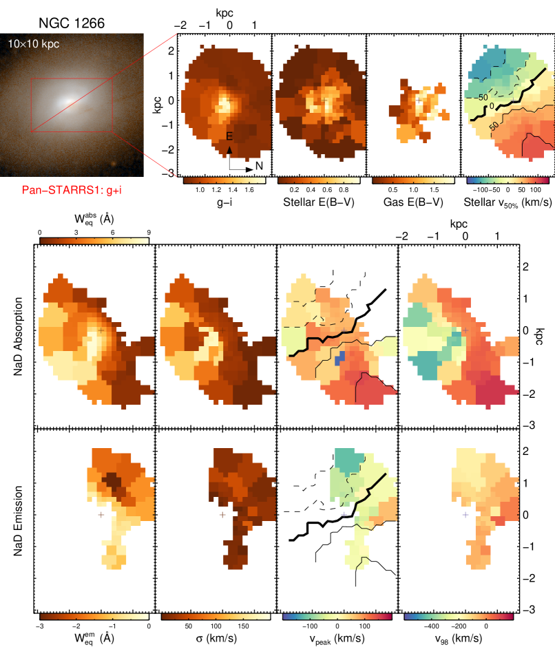
Figure 1: Images and maps of stellar and gas properties of each galaxy (Table 2 and Section 2). Top row, left: 2-colour image, with telescope and filters labeled below. The WiFeS FOV (25″$\times$38″) is outlined in red. Top row, middle and right: Maps of broadband colour, stellar colour excess, ionized gas colour excess, and stellar velocity. Spaxel sizes are 1$\aas@@fstack{\prime\prime}$0. Broadband images are rebinned to match the Voronoi tessellation of the IFS data of each galaxy to compute colours. The stellar and gas properties are derived from fits to the data. The cross marks the continuum peak used to register the images and IFS maps, and distances from the peak are shown in kpc on the left and top axis of the colour map. Lines in the rightmost panel are isovelocity contours. Middle and bottom rows: Equivalent width $W_{\mathrm{eq}}$, velocity dispersion $\sigma$, velocity at peak optical depth $v_{\mathrm{peak}}$, and maximum velocity $v_{98\%}$ of Na I D absorption and emission lines, in Å and km s^-1. We derive these quantities from one-component fits except for the absorption lines in NGC 1266 and NGC 1808, for which we use two components in some spaxels. For one-component fits, $\sigma$ has the usual Gaussian definition and $v_{98\%}\equiv v_{50\%}-2\sigma$, where $v_{50\%}=v_{\mathrm{peak}}$ is the central velocity. For two-component fits, the velocities are derived from the cumulative velocity distribution in optical depth space, as described in the text. On the $v_{\mathrm{peak}}$ map, lines are the stellar isovelocity contours. The full set is available online.

The Indo-US library contains 1273 spectra. However, we only need representative stars across the range of stellar properties. We first select spectra that have full coverage between 3465 Å and 7000 Å with any gaps in coverage smaller than 50 Å, suitable for fitting the S7 data. We also require measurements of effective temperature $T_{\mathrm{eff}}$, gravity log $g$, and metallicity [Fe/H]. This narrows the list to 1148 stars. Next, we evenly grid the resulting spectra into bins of log $g$ and [Fe/H], with log $g$ ranging from 0 to 5 in bins of 0.25 and [Fe/H] ranging from $-$1 to 0.4 in units of 0.2. This captures the bulk of the distribution of these parameters in the Indo-US catalog. We then add the tail of high-metallicity, high-temperature (and high log $g$) stars by gridding in log $T_{\mathrm{eff}}$ from 3.9 to 4.5 in units of 0.1 and over the same range in metallicity. Finally, we take one star at random from each bin and add it to our library. The final template library of 123 stars samples a wide range in stellar properties.

The native pixel dispersions out of the S7 reduction pipeline are 0.76 and 0.44 Å in the blue and red, respectively. We resample them to 0.88 Å and stitch the two spectra at 5600 Å. (The resampling and stitching routine is part of the IFSRED library; Rupke 2014a.)

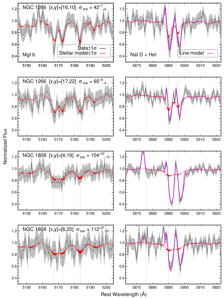
Figure 2: Four examples of inverse P Cygni profiles in our data. Each row represents a Voronoi bin in a data cube, with the bin labeled by one of its spaxels at column and row $[x,y]$, with spaxel $[1,1]$ at lower left and $[25,38]$ at upper right. Left: Region around the Mg I b stellar lines; wavelengths are in the rest frame of the stars in the given spaxel. Black lines and grey shaded regions are the data and 1$\sigma$ error. Red area is the range of models given the best-fit stellar velocity dispersion $\sigma_{\star}$ and its 1$\sigma$ error. Dashed lines locate Mg I b. Right: Region around Na I D. As at left, red area is the range of stellar models. Magenta lines show the best-fit Na I D $+$ He I 5876 Å ISM model after subtraction of the stellar model. The expected locations of Na I D and He I based on the stellar velocity at each location are shown with vertical dashed lines. In each case the Na I D emission doublet is blueshifted from the stellar velocity and the Na I D absorption is redshifted.

We then fit the entire available spectral range of the Voronoi tessellated data cubes using IFSFIT (Rupke, 2014b) and the Indo-US stellar templates. IFSFIT iteratively fits the stellar continuum and ionized gas emission lines. In each Voronoi bin, it does the following in order: masks potential interstellar features (emission lines and the Na I D doublet); fits the stellar continuum with PPXF (Cappellari & Emsellem, 2004; Cappellari, 2012); subtracts the continuum; and fits emission lines. It then repeats this process with more refined initial conditions based on the first fit.

Before performing the stellar continuum fits, we match the templates and data in spectral resolution to ensure that the fitted velocity dispersion is accurate. In the blue we convolve the template with a Gaussian for which the sigma equals the wavelength-dependent difference in resolution between the data and templates. In the red, we convolve the data to match the templates. Further fitting steps act on the unconvolved data after normalization by the continuum model. To account for residual calibration errors across the wide FOV, we include an additive 4th-order Legendre polynomial as part of the continuum model. For 5/8 galaxies, we increase the default polynomial order from 4 to 10 because of larger residuals. We assume a symmetric, Gaussian line-of-sight stellar velocity distribution ($MOMENT=2$ in the call to PPXF). We fit stellar color excess using the PPXF option to apply the Calzetti et al. (2000) reddening curve with $R_{V}=4.05$ to the continuum. Finally, in each Voronoi bin, we fit errors in the recovered stellar parameters—velocity $v_{\star}$, velocity dispersion $\sigma_{\star}$ and colour excess $E(B-V)$_⋆. To do so, we run a 100-iteration Monte Carlo simulation of the best-fit stellar continuum. Using the resulting distributions of best-fit $v_{\star}$, $\sigma_{\star}$ and $E(B-V)$_⋆, we calculate the two-sided 1$\sigma$ errors on each parameter from the 34$\%$ interval on either side of the median.

The stellar fits are of high quality. The median 1$\sigma$ errors in the stellar parameters, where the median is taken over the Voronoi bins in each data cube, range over 8–15 km s^-1 in $v_{\star}$, 8–18 km s^-1 in $\sigma_{\star}$ and 0.08–0.12 in $E(B-V)$_⋆. The velocity errors are low compared to the spectral resolution of 100 (43) km s^-1 in the red (blue). The large wavelength range of the fit ensures that numerous spectral lines—both strong and weak—strongly constrain the fit and produce an excellent match between data and model throughout the dataset. This can be seen visually in the regular appearance of the $v_{\star}$ maps (Figure 1) and in the good agreement of the data and model in the wavelength region around Mg I b (Figure 2). The Na I D and Mg I b stellar strengths are strongly correlated in most galaxies (e.g., Jeong et al., 2013). Finally, visual comparison to published stellar velocity maps show a good match in NGC 1266 (Krajnović et al., 2011), NGC 1808 (Busch et al., 2017), and NGC 5728 (Shin et al., 2019).

We choose a redshift that produces the best antisymmetry around the $v_{\star}=0$ km s^-1 contour in the maps of $v_{\star}$ (Cappellari et al., 2011). We then apply a heliocentric correction computed with the IDL routine BARYVEL (Stumpff, 1980; Landsman, 1993) These are reported in Table 1, and have 1$\sigma$ errors of $\delta z=0.00002$. In this study, all velocities for each galaxy are computed with respect to its systemic velocity.

Systematic errors in Na I D stellar fitting could arise due to choice of stellar template. Chen et al. (2010) find no significant effects on their study of Na I D in SDSS between two choices of stellar models. We tested systematic uncertainties due to template choice by choosing a different subset of the Indo-US models; this has no effect. We also compared to fits using the González Delgado et al. (2005) models; while less suited to this analysis due to the resolution mismatch (as we discuss above), they are used in the default S7 pipeline fits. Again, this change has almost no effect. The strength of the stellar Na I D feature can also increase relative to Mg I b due to [Na/Fe] abundance variations. However, this effect is seen only in massive, early-type galaxies, not in the early-type spirals like those in our sample (Jeong et al., 2013).

The deep S7 data contain a wealth of emission lines (Thomas et al., 2017). These include the usual strong lines found in the rest-frame optical and fainter lines typically found in Seyfert nuclei. In particular, He I 5876 Å lies just blueward of Na I D and can blend with the Na I D profile. We discuss this line further below.

We constrain all visible lines in each bin to have the same velocity and velocity dispersion. Before fitting, we convolve each emission-line model with the wavelength-dependent spectral resolution of the data. We assume two velocity components as a baseline in most bins; components with S/N < 2$\sigma$ are dropped and the spectrum is re-fit. A third component is added in a few bins in NGC 5728 and IC 1481. In bins where both H$\alpha$ and H$\beta$ are detected, we use the Balmer decrement to calculate colour excess $E(B-V)$_gas assuming H$\alpha$/H$\beta=3.1$, appropriate for Seyfert galaxies (Kewley et al., 2006; Thomas et al., 2018), and $R_{V}=4.05$.

Finally, we fit the Na I D absorption and emission lines following procedures outlined in previous work (Rupke et al., 2005a; Shih & Rupke, 2010; Rupke & Veilleux, 2015). We set the upper bound of the peak optical depth in the D₁ line to $\tau_{5896}=5$; best-fit values of $\tau_{5896}=5$ are considered lower limits. To avoid the inevitable degeneracy between emission and absorption line components in Voronoi bins where both arise, we first fit Na I D emission and then absorption. This likely underestimates the equivalent width ($W_{\mathrm{eq}}$) and line width $\sigma$ in both emission and absorption where both are present and overlapping. Progress in modeling resonant line features with simulations or other gas phases (e.g., Baron et al., 2020) may alleviate this difficulty. Each line model is convolved with the spectral resolution of the data before fitting. The lower limit for intrinsic linewidth $\sigma$ is set to 1 km s^-1, which is approximately the thermal value for Na atoms at 1000–6000 K. We fit one velocity component to every Na I D emission line. The emission-line flux ratio $f(5890$ Å$)/f(5896$ Å) is allowed to vary between 1 and 2. We fit one component to every absorption line except in NGC 1266 and NGC 1808, where two absorption lines are fit in the nuclear regions and small off-nuclear regions. Fits of either absorption lines or emission lines with S/N $<2$ in equivalent width are discarded. To estimate errors, we perform 200-iteration Monte Carlo simulations in each Voronoi bin. As in computing stellar errors, we calculate the two-sided 1$\sigma$ errors on each parameter from the 34$\%$ interval on either side of the median.

We fit and remove He I 5876 Å emission during continuum and emission-line fitting for all galaxies but NGC 1266 and NGC 1808. Neither has a Seyfert optical spectral type (Table 1) or low metallicity, so He emission lines are weak. NGC 1266 also has the broadest and deepest Na I D absorption and NGC 1808 has the highest S/N data. In these two cases we fit He I 5876 Å and Na I D simultaneously. We constrain He I 5876 Å to have the same velocity and linewidth as other emission lines, and its flux is determined as part of the Na I D fitting.

Example Na I D fits are shown in Figure 2. These Voronoi bins are chosen to showcase inverse P Cygni profiles, which we discuss further in Sections 4 and 5 below. They illustrate that the inverse P Cygni profiles we detect are often visible prior to stellar continuum subtraction.

Table 2: Imaging data. The image sources are PS1 = Panoramic Survey Telescope and Rapid Response System Data Release 1 (Pan-STARRS1 DR1), CGS = Carnegie-Irvine Galaxy Survey (Ho et al., 2011), SSS = SkyMapper Southern Sky Survey DR3 (Wolf et al., 2018), and ATLAS = VLT Survey Telescope (VST) ATLAS Data Release 3 (DR3; Shanks et al. 2015). Exposure times in $g$ and $i$ filters are given in s. Seeing for CGS, SSS, and ATLAS is measured by the survey; we estimate PS1 seeing from stars in the field. $i$ images are convolved to match $g$ seeing if they differ by more than 0$\aas@@fstack{\prime\prime}$1. The correction for Galactic reddening $\Delta^{g-i}_{\mathrm{Gal}}$ is given, from Schlafly & Finkbeiner (2011) as implemented at https://irsa.ipac.caltech.edu/applications/DUST/. Other colour corrections $\Delta^{g-i}_{\mathrm{other}}$ are also listed. For SSS, the colour correction is from the SkyMapper to SDSS $g$ filters based on $g-i=1.0$. For ATLAS, the correction is from Vega to AB magnitudes (Hewett et al., 2006).

Galaxy	Source	$t_{\mathrm{exp}}$	Seeing	$\Delta^{g-i}_{\mathrm{Gal}}$	$\Delta^{g-i}_{\mathrm{other}}$
NGC 1266	PS1	860/1800	1$\aas@@fstack{\prime\prime}$4	-0.16	—
NGC 18081	CGS	360/180	1$\aas@@fstack{\prime\prime}$0	-0.06	—
ESO 500-G34	PS1	654/1298	1$\aas@@fstack{\prime\prime}$2	-0.09	—
NGC 5728	PS1	638/1118	1$\aas@@fstack{\prime\prime}$2	-0.16	—
ESO 339-G11	SSS	5/100	3$\aas@@fstack{\prime\prime}$0	-0.17	0.3
IC 5063	SSS	100/100	2$\aas@@fstack{\prime\prime}$8	-0.10	0.3
IC 5169	ATLAS	100/90	0$\aas@@fstack{\prime\prime}$8	-0.03	-0.46
IC 1481	PS1	946/1920	1$\aas@@fstack{\prime\prime}$2	-0.12	—

• Filters for NGC 1808 are $B$ and $I$ rather than $g$ and $i$; quantities in this table refer to $B$ and $I$ filters.

Broad-band optical images are available from various surveys (Table 2). We use the deepest images that permit calculation of $g-i$ colour as a proxy for stellar attenuation. (The exception is NGC 1808, for which only $B-I$ colour is available.) We sky-subtract and photometrically calibrate these images as necessary, and convolve them to match the seeing of the WiFeS observations if the WiFeS seeing is worse. As in Rupke & Veilleux (2013), we register the images and data cube for each galaxy by computing the flux peak of the combined $g+i$ ($B+I$ for NGC 1808) image and an image created by stacking the data cube over all wavelengths. We compute the peaks using 2d, circular Moffat fits to the central pixels of each image with the IDL routine MPFIT2DPEAK (Markwardt, 2009). We then apply shifts to the images to align their peak to the data cube. The images, along with cutouts corresponding to the WiFeS FOV, are shown in Fig. 1. This figure also shows maps of colour, $E(B-V)$_⋆, $E(B-V)$_gas, and v_⋆.

The distributions of Na I D absorbing and emitting gas in each galaxy are shown as $W_{\mathrm{eq}}$ maps in the lower panels of Fig. 1. These panels also present the linewidth, peak velocity, and 98% velocity ($v_{98\%}$) of the cumulative velocity distribution (CVDF) of absorbing and emitting gas. As in Rupke et al. (2017), we construct the CVDF in optical depth space for absorption lines and compute velocities for which a specified percentage of the CVDF area is redshifted from that velocity. For instance, 50% of the CVDF lies blue- and redward of $v_{50\%}$, and 98% of the CVDF lies redward of $v_{98\%}$. The velocity dispersion is defined as $\sigma\equiv(v_{16\%}-v_{84\%})/2$. For the Na I D emission and single-component Na I D absorption fits, the central velocity $v_{50\%}$ equals the velocity at the peak of the CVDF, $v_{\mathrm{peak}}$ and $v_{98\%}\equiv v_{50\%}-2\sigma$.

3 Spatially resolving the cool, neutral gas and dust connection

The strong correlations between Na I D absorption and colour excess derived from gas measurements along stellar and QSO sightlines through the Milky Way’s ISM and halo have been studied for decades (Hobbs, 1974; Sembach et al., 1993; Sembach & Danks, 1994; Welty et al., 1994; Richmond et al., 1994; Munari & Zwitter, 1997; Wakker & Mathis, 2000; Welty & Hobbs, 2001; Poznanski et al., 2012; Murga et al., 2015). Na I D traces dusty, cool, neutral gas in the diffuse ISM through the disk; this gas (traced by H I, Na I, and reddening) has scale heights 0.4–0.5 kpc (Sembach & Danks, 1994). These studies find that Na I absorption $W_{\mathrm{eq}}$ and/or column density scale with $E(B-V)$_gas and/or N(H I). There is significant scatter among sightlines (Wakker & Mathis, 2000; Murga et al., 2015) due to varying ionization conditions and linewidths. High spectral resolution finds complexes of low-$\sigma$ ($\sigma<10$ km s^-1) clouds (Hobbs, 1974; Sembach et al., 1993) that may comprise a dusty and cold neutral medium of compact clouds (Werk et al., 2019; Peek & Clark, 2019). These Galactic sightlines are thus primarily sensitive to low-to-moderate column densities ($N($Na I$)\la 10^{12.5}$ cm^-2 and $N($H I$)\la 10^{20.5}$ cm^-2) and colour excess values $E(B-V)_{\mathrm{gas}}\la 0.3$. Stacking analyses increase the ranges of $E(B-V)$ probed, but $W_{\mathrm{eq}}$ still saturates at $\sim$1 Å at $E(B-V)_{\mathrm{gas}}\ga 0.2$ (Poznanski et al., 2012).

These correlations extend to external galaxies. Single-aperture studies of both infrared- and optically-selected galaxies find strong correlations between nuclear $E(B-V)$_gas and Na I D absorption-line $W_{\mathrm{eq}}$ (Veilleux et al., 1995; Chen et al., 2010). Because these sightlines trace larger projected areas, they encompass many more clouds moving at a much wider range of velocities. They thus have larger linewidths, equivalent widths, and column densities, but often covering factors well below unity (Heckman et al., 2000; Rupke et al., 2005a, b). A notable exception are the host galaxy absorbers in front of Type 1 QSOs (Baron et al., 2016), for which the background source has a small projected area as seen by the host galaxy absorber (though not perfectly point-like). These host galaxy absorbers also have equivalent widths and column densities that correlate with reddening (Baron et al., 2016).

Spatially-resolved correlations between Na I D equivalent width and continuum colour also exist in 2–3 nearby galaxies that are notably dusty and have strong neutral outflows (Shih & Rupke, 2010; Rupke & Veilleux, 2013, 2015). Resonant emission in Na I D may in turn escape along low $E(B-V)$ sightlines (Rupke & Veilleux, 2015). However, in at least one another system (NGC 5626), there is no connection between Na I D and dust attenuation (Viaene et al., 2017).

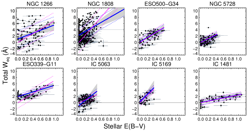
Figure 3: Total (absorption$+$emission) fitted Na I D equivalent width vs. stellar colour excess, as measured from stellar continuum fitting. The solid blue and magenta lines are linear fits to the data with intrinsic Gaussian scatter using LINMIX_ERR and MPFITEXY.

The gray area shows 2$\sigma$ deviations from the median LINMIX_ERR fit after applying the posterior distributions of slopes and intercepts to the measured dependent variables. The dashed lines show the best fit lines plus fitted scatter. Regression models are shown only for those cases where the correlation is statistically significant at the 2$\sigma$ level. Data points are shown with 1$\sigma$ errors.

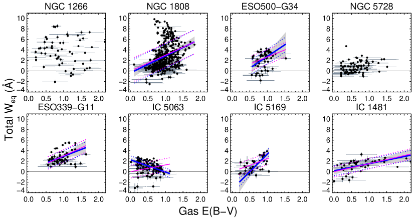
Figure 4: Total fitted Na I D equivalent width vs. colour excess, as measured from the Balmer decrement. See Fig. 3 caption for more details.

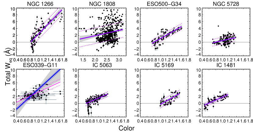
Figure 5: Total fitted Na I D equivalent width vs. $g-i$ colour ($B-I$ colour for NGC 1808 only). See Fig. 3 caption for more details.

Table 3: Fits to $W_{\mathrm{eq}}$ vs. stellar $E(B-V)$. Columns are sample size N; correlation coefficient $r_{xy}$; and regression intercept, slope, and intrinsic scatter. $p$-values are given in parentheses next to $r_{xy}$; many $p$-values are upper limits due to finite sampling of the correlation coefficient PDF. 1$\sigma$ errors are given for other quantities. The assumed model is $W_{\mathrm{eq}}=m[E(B-V)]+$$W_{\mathrm{eq}}$${}_{0}+\delta W_{\mathrm{eq}}$, where m is the constant slope in Å, $W_{\mathrm{eq}}$₀ is the equivalent width at $E(B-V)=0$ in Å, and $\delta$$W_{\mathrm{eq}}$ (in Å) is normally distributed. For each galaxy, the first row lists the results from a Bayesian regression with LINMIX_ERR. The second row is from a regression with MPFITEXY with $W_{\mathrm{eq}}$₀ fixed to zero.

Galaxy	N	$r_{xy}$	$W_{\mathrm{eq}}$0	$m$	$\delta$$W_{\mathrm{eq}}$
NGC 1266	99	0.37 (0.0001)	1.14${}_{-0.51}^{+0.51}$	4.58${}_{-1.36}^{+1.35}$	2.64${}_{-0.19}^{+0.23}$
			0.0	7.08$\pm$0.65	2.73$\pm$0.19
NGC 1808	503	0.40 (<6e-5)	2.31${}_{-0.11}^{+0.11}$	6.92${}_{-1.02}^{+1.00}$	2.15${}_{-0.07}^{+0.08}$
			0.0	13.68$\pm$2.84	3.14$\pm$0.09
ESO500-G34	73	0.77 (<6e-5)	0.15${}_{-0.24}^{+0.23}$	7.17${}_{-0.85}^{+0.94}$	1.01${}_{-0.10}^{+0.14}$
			0.0	7.50$\pm$0.49	1.29$\pm$0.11
NGC 5728	130	0.59 (<6e-5)	0.05${}_{-0.13}^{+0.15}$	5.77${}_{-1.16}^{+0.92}$	0.83${}_{-0.07}^{+0.08}$
			0.0	6.33$\pm$0.78	1.00$\pm$0.10
ESO339-G11	74	0.79 (<6e-5)	1.98${}_{-0.12}^{+0.12}$	3.67${}_{-0.49}^{+0.46}$	0.68${}_{-0.09}^{+0.12}$
			0.0	7.28$\pm$0.33	1.70$\pm$0.10
IC 5063	148	0.62 (<6e-5)	-0.90${}_{-0.64}^{+0.47}$	9.49${}_{-2.52}^{+3.44}$	0.83${}_{-0.09}^{+0.10}$
			0.0	5.29$\pm$0.53	1.16$\pm$0.06
IC 5169	47	0.78 (<6e-5)	0.30${}_{-0.22}^{+0.24}$	11.99${}_{-2.65}^{+2.93}$	0.83${}_{-0.16}^{+0.24}$
			0.0	11.55$\pm$1.37	1.09$\pm$0.16
IC 1481	59	0.74 (<6e-5)	0.05${}_{-0.17}^{+0.17}$	2.45${}_{-0.36}^{+0.37}$	0.73${}_{-0.09}^{+0.12}$
			0.0	2.49$\pm$0.20	0.84$\pm$0.07

Table 4: Fits to $W_{\mathrm{eq}}$ vs. gas $E(B-V)$. See Table 3 for more details.

Galaxy	N	$r_{xy}$	$W_{\mathrm{eq}}$0	$m$	$\delta$$W_{\mathrm{eq}}$
NGC 1266	59	-0.02 (0.5)	3.80${}_{-0.88}^{+0.91}$	-0.09${}_{-0.84}^{+0.85}$	2.60${}_{-0.22}^{+0.29}$
			0.0	3.09$\pm$0.37	3.07$\pm$0.21
NGC 1808	458	0.29 (<6e-5)	-0.37${}_{-0.56}^{+0.57}$	3.23${}_{-0.56}^{+0.55}$	2.29${}_{-0.08}^{+0.08}$
			0.0	3.02$\pm$0.11	2.25$\pm$0.09
ESO500-G34	59	0.45 (0.01)	-1.68${}_{-1.54}^{+1.67}$	4.45${}_{-1.90}^{+1.71}$	1.37${}_{-0.15}^{+0.19}$
			0.0	2.67$\pm$0.20	1.39$\pm$0.13
NGC 5728	82	0.24 (0.05)	0.04${}_{-0.40}^{+0.42}$	1.14${}_{-0.65}^{+0.64}$	1.03${}_{-0.08}^{+0.10}$
			0.0	1.30$\pm$0.17	1.02$\pm$0.12
ESO339-G11	59	0.46 (0.002)	0.36${}_{-0.78}^{+0.77}$	2.58${}_{-0.85}^{+0.89}$	1.11${}_{-0.11}^{+0.13}$
			0.0	3.02$\pm$0.21	1.20$\pm$0.11
IC 5063	140	-0.58 (<6e-5)	2.27${}_{-0.22}^{+0.21}$	-2.33${}_{-0.34}^{+0.35}$	0.75${}_{-0.06}^{+0.07}$
			0.0	1.29$\pm$0.15	1.20$\pm$0.06
IC 5169	43	0.84 (<6e-5)	-3.35${}_{-1.17}^{+0.94}$	6.69${}_{-1.26}^{+1.51}$	0.76${}_{-0.14}^{+0.18}$
			0.0	2.45$\pm$0.27	1.11$\pm$0.08
IC 1481	43	0.59 (0.0008)	0.17${}_{-0.34}^{+0.34}$	1.35${}_{-0.38}^{+0.37}$	0.92${}_{-0.12}^{+0.16}$
			0.0	1.54$\pm$0.16	0.99$\pm$0.09

Table 5: Fits to $W_{\mathrm{eq}}$ vs. $g-i$ colour. See Table 3 for more details. In this case, $(g-i)_{0}$ is the x-intercept computed from the fitted y-intercept, and the y-intercept is not fixed to zero in either regressions.

Galaxy	N	$r_{xy}$	$(g-i)_{0}$	$m$	$\delta$$W_{\mathrm{eq}}$
NGC 1266	99	0.83 (<6e-5)	0.82${}_{-0.09}^{+0.09}$	10.36${}_{-0.69}^{+0.72}$	1.53${}_{-0.11}^{+0.13}$
			0.82$\pm$0.10	10.40$\pm$0.80	1.54$\pm$0.14
NGC 1808	503	0.19 (<6e-5)	0.78${}_{-0.63}^{+0.65}$	1.56${}_{-0.37}^{+0.37}$	2.30${}_{-0.07}^{+0.08}$
			0.78$\pm$0.72	1.55$\pm$0.42	2.27$\pm$0.08
ESO500-G34	73	0.83 (<6e-5)	0.80${}_{-0.12}^{+0.12}$	5.64${}_{-0.48}^{+0.49}$	0.89${}_{-0.08}^{+0.10}$
			0.80$\pm$0.11	5.63$\pm$0.40	0.87$\pm$0.10
NGC 5728	130	0.32 (<6e-5)	0.79${}_{-0.36}^{+0.34}$	2.27${}_{-0.58}^{+0.61}$	0.98${}_{-0.06}^{+0.07}$
			0.79$\pm$0.35	2.28$\pm$0.60	0.97$\pm$0.09
ESO339-G11	74	0.93 (<6e-5)	0.59${}_{-0.23}^{+0.23}$	9.15${}_{-1.96}^{+1.92}$	0.41${}_{-0.13}^{+0.22}$
			0.33$\pm$0.56	4.64$\pm$2.77	0.90$\pm$0.24
IC 5063	148	0.74 (<6e-5)	0.63${}_{-0.09}^{+0.09}$	4.32${}_{-0.34}^{+0.34}$	0.64${}_{-0.05}^{+0.06}$
			0.64$\pm$0.09	4.36$\pm$0.32	0.72$\pm$0.08
IC 5169	47	0.68 (<6e-5)	1.04${}_{-0.30}^{+0.31}$	5.67${}_{-1.06}^{+1.04}$	1.04${}_{-0.11}^{+0.15}$
			1.05$\pm$0.25	5.68$\pm$0.85	0.99$\pm$0.10
IC 1481	59	0.85 (<6e-5)	0.58${}_{-0.10}^{+0.10}$	4.45${}_{-0.42}^{+0.44}$	0.57${}_{-0.07}^{+0.09}$
			0.59$\pm$0.09	4.49$\pm$0.40	0.57$\pm$0.06

• Filters for NGC 1808 are $B$ and $I$ rather than $g$ and $i$; quantities in this table refer to $B$ and $I$ filters.

For one well-resolved source, Rupke & Veilleux (2015) use a spatial model of dust and Na I D that separates the emission and absorption line contributions to the equivalent width in each spaxel. This sample is of larger size and our interest lies in looking for correlations with model-independent observables. Here we choose a simpler approach and use total equivalent width ($W_{\mathrm{eq}}^{\mathrm{abs}}+W_{\mathrm{eq}}^{\mathrm{em}}$) as a proxy that includes both within each Voronoi bin. However, the number of points in which both are present is a small fraction of the total and the relationships are driven by points in which one or the other is present.

Our data allow us to quantify the spatially-resolved connection between Na I D equivalent width and dust across the disks in our subsample. Fig. 3–5 display the relationship between total equivalent width ($W_{\mathrm{eq}}^{\mathrm{abs}}+W_{\mathrm{eq}}^{\mathrm{em}}$) and stellar $E(B-V)$, gas $E(B-V)$, and $g-i$ colour for each galaxy. There is significant intrinsic scatter in these plots unaccounted for by the measurement errors, so as in Rupke et al. (2017) we compute Bayesian linear regressions using LINMIX_ERR (Kelly, 2007). Based on samples of the posterior probability distribution functions (PDFs), we list the median and $p$-value for the correlation coefficient and median and 1$\sigma$ errors for intercept, slope and instrinsic scatter in Tables 3–5. Many $p$-values are upper limits due to finite sampling of the correlation coefficient PDF.

For comparison, we also compute regressions using MPFITEXY (Williams et al., 2010) and find the resulting errors in slope and intrinsic scatter using a simple 1000-sample bootstrap (Hogg et al., 2010). We enable the option to adjust the intrinsic scatter to produce $\chi_{r}\sim 1$ (Bedregal et al., 2006). Here, we also fix the y-intercept to zero for $W_{\mathrm{eq}}$ vs. $E(B-V)$ for comparison to the unfixed values in the LINMIX_ERR fits. It is unclear whether or not total $W_{\mathrm{eq}}$ should be zero at $E(B-V)=0$; Chen et al. (2010) find that $W_{\mathrm{eq}}<0$ at $E(B-V)=0$, while in Poznanski et al. (2012) the intercept is consistent with zero. For the $W_{\mathrm{eq}}$ vs. $g-i$ fit, we list the x-intercept, which should relate to the intrinsic colour of the galaxy at low colour excess.

The neutral gas and dust show statistically significant correlations throughout; $r_{xy}>0$ at the 95.5% (99.99%) level in 22/24 (18/24) fits. The significance and strengths of these correlations are highest for $W_{\mathrm{eq}}$ vs. $E(B-V)$_⋆ and $g-i$. We find a median $r_{xy}$ of 0.74 and 0.83 for $W_{\mathrm{eq}}$ with $E(B-V)$_⋆ and $g-i$, respectively, vs. 0.45 for $W_{\mathrm{eq}}$ with $E(B-V)$_gas. There is intrinsic scatter in these correlations, however, with a median value across the sample (and across fitting methods) of 1.0 Å.

The results from the two fitting methods produce very consistent results, in particular for the $g-i$ fits. Differences appear largely from fixing the y-intercept in MPFITEXY in the $E(B-V)$ fits, though in cases where the fitted intercept with LINMIX_ERR is near zero the slopes are consistent. The covariance between slope and intercept is evident in that, for any galaxy, larger best-fit slopes result from the fit (LINMIX_ERR or MPFITEXY) with smaller intercept, and vice versa. The parameter errors are typically larger from LINMIX_ERR than those from the bootstrap errors with MPFITEXY, while the fitted intrinsic scatter is in turn lower. This points to differences in how the methods (LINMIX_ERR and MPFITEXY with bootstrap errors) treat the tradeoff between parameter errors and intrinsic scatter.

When the median and standard deviation in the slope is taken over all galaxies for each type of correlation and each fitting method, the methods differ primarily in that the MPFITEXY method produces much lower variance for $W_{\mathrm{eq}}$ vs. $E(B-V)$_gas. Taking the method with the lowest variance for each type of correlation, the values for median slope and standard deviation across the 8-galaxy sample are (6.9$\pm$3.1) Å, (2.7$\pm$0.8) Å, and (4.6$\pm$2.7) Å for $W_{\mathrm{eq}}$ vs. $E(B-V)$_⋆, $E(B-V)$_gas, and $g-i$, respectively. As a physical sanity check, the ratio of the median slopes from the fits to $E(B-V)$_gas and $E(B-V)$_⋆, $m(E(B-V)_{\mathrm{gas}})/m(E(B-V)_{\star}$, is 0.39$\pm$0.07. This ratio of slopes is consistent with the average ratio of stellar to gas colour excess, $E(B-V)_{\star}/E(B-V)_{\mathrm{gas}}$, for which the canonical value is 0.44$\pm$0.03 (Calzetti et al., 2000; Kreckel et al., 2013), though this can vary from galaxy to galaxy and within galaxies (Greener et al., 2020).

For half of the sample (ESO 500-G34, ESO 339-G11, IC 5169, and IC 1481) the correlations between $W_{\mathrm{eq}}$ and dust measure ($E(B-V)$_⋆, $E(B-V)$_gas, or $g-i$) are consistently strong ($r_{xy}\ga 0.5$) and significant among all three dust measures. In other galaxies the situation is less clear. In NGC 1266, the strongest and most signficant correlation, with the lowest scatter in regression, is $W_{\mathrm{eq}}$ vs. $g-i$. The $W_{\mathrm{eq}}$ vs. $E(B-V)$_⋆ correlation is weaker and the fit has larger scatter, while $W_{\mathrm{eq}}$ and $E(B-V)$_gas show no correlation at all. NGC 1266 also has the steepest fitted slope of any galaxy in $W_{\mathrm{eq}}$ vs. colour space. In IC 5063, $W_{\mathrm{eq}}$ correlates strongly and significantly with $E(B-V)$_⋆ and colour, but has a strong anti-correlation with $E(B-V)$_gas. The colour map reflects the strong dust lane running NW to SE across the near side (NE) of the galaxy, which is also where the Na I D $W_{\mathrm{eq}}$ is highest, while $E(B-V)$_gas shows strong obscuration away from the dust lane and low obscuration in the dust lane (Figure 1$f$). NGC 1808 has weak (though significant) correlations in all three relationships but very large scatter ($r=0.2-0.4$ and $\delta W_{\mathrm{eq}}>2.3$ Å). It is the nearest and best-resolved galaxy in our sample, and the high S/N data record spatially-resolved patterns that are not best described with linear relationships. Finally, in NGC 5728 there is a region of scattered AGN light (Capetti et al., 1996) that skews the colour map, so that the stellar $E(B-V)$ correlation is strongest.

As a final sanity check, the x-intercepts of the $g-i$ fits should be consistent with observed intrinsic stellar colours. The S7 galaxies have masses $M_{\star}=10^{10-11}~{}M_{\odot}$ and lie mostly in the blue sequence or green valley. Integrated unattenuated colours from the Galaxy And Mass Assembly (GAMA) survey are in the range 0.2–0.8 for $M_{\star}=10^{10-11}~{}M_{\odot}$ blue sequence galaxies, and a bit higher for the green valley (Taylor et al., 2015). Our measured $(g-i)_{0}$ are consistent with, but fall toward the high end of, these values, with a median of 0.8 and a range of 0.3–1.0.

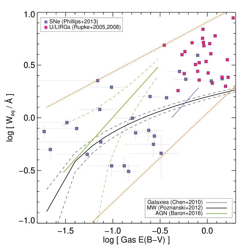
Figure 6: Na I D absorption equivalent width vs. colour excess of ionized gas in the Milky Way and external galaxies. Purple and magnenta squares show individual sightlines to supernovae (Phillips et al., 2013) and infrared-luminous galaxies (Rupke et al., 2005a, 2008). Lines show fits to the relationship between these quantities for SDSS star-forming galaxies (Chen et al., 2010, purple solid line), AGN (Baron et al., 2016, green solid line), and Milky Way sightlines to background galaxies and quasars (Poznanski et al., 2012, black solid line). Dashed lines delineate 1$\sigma$ uncertainties in the fits, while gray lines show 1$\sigma$ errors in data points. The orange dotted lines show the approximate range of the data and fits.

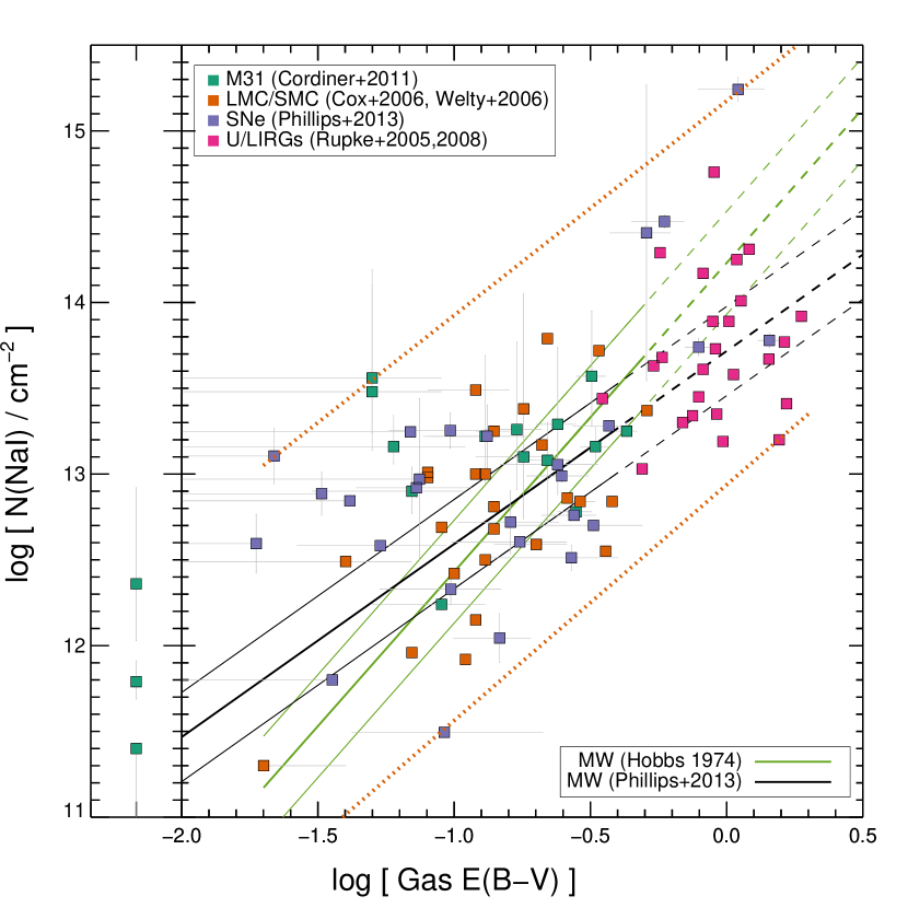
Figure 7: Na I D absorption column density vs. colour excess of ionized gas in the Milky Way and external galaxies. In addition to the sightlines through infrared-luminous galaxies (pink squares) and galaxies containing supernovae (purple) shown in Fig. 6, sightlines to bright stars in M31 (green) and the LMC/SMC (orange) are shown. Green and black lines show fits to Milky Way data $\pm$1$\sigma$ (Hobbs, 1974; Phillips et al., 2013), and dashed lines are extensions of these relationships to higher $E(B-V)$_gas. Dotted orange lines show the approximate range of the data.

To contextualize these results, we explore where our data lie in $W_{\mathrm{eq}}^{\mathrm{abs}}$ and $N$(Na I) vs. $E(B-V)$_gas space. We calculate column density as in Rupke et al. (2005a), and where the best-fit D₁ optical depth is a lower limit ($\tau_{5896}\geq 5$) we consider the column density to be a lower limit. We compare to the extensive measurements in the Milky Way, which largely probe low extinctions, and the limited set of sightlines in external galaxies that reach higher $E(B-V)$. The most recent study of MW sightlines uses both stars and background galaxies/quasars (Poznanski et al., 2012) to derive a high-precision average $W_{\mathrm{eq}}^{\mathrm{abs}}$ vs. $E(B-V)$ (Fig. 6). External galaxy sightlines (backlit by point sources like AGN/supernovae or nuclear starbursts) straddle this relationship but often lie above it by factors up to 0.6 dex, particlarly at $E(B-V)\ga 0.5$ (Rupke et al., 2005a, 2008; Chen et al., 2010; Phillips et al., 2013; Baron et al., 2016). Two fits to MW stellar measurements of $N$(Na I) and $E(B-V)$, despite being made 40 years apart, yield roughly the same result (Fig. 7). Most external galaxy measurements lie roughly in the extrapolation of these fits, with a possible tendency to scatter above rather than below them.

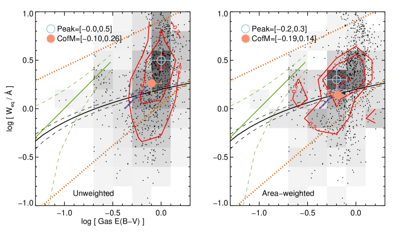
Figure 8: Na I D absorption equivalent width vs. colour excess from gas measurements in our sample, compared to MW and other external galaxy sightlines. Black circles are individual Voronoi bins. The spatial bins are binned in $W_{\mathrm{eq}}$ vs. $E(B-V)$ space and the grey shading of each bin represents the number of Voronoi bins within a plot bin. The binning on the left is unweighted, while on the right bins are first weighted by the projected area they subtend on the galaxy. Red contour lines of 0.2, 0.4, and 0.8 represent (weighted) number of spaxels in each Voronoi bin divided by the value in the peak bin. The light blue open and light red filled circles are the peak and "center-of-mass" of the binned data. The other lines are as described in Fig. 6. Our data are on average consistent with single-apertures sightlines through the Milky Way and external galaxies, though they probe to both lower and higher $W_{\mathrm{eq}}$ values for a given $E(B-V)$.

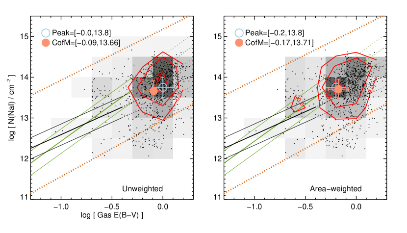
Figure 9: Na I D absorption column density vs. colour excess from gas measurements in our sample, compared to MW and other external galaxy sightlines. See Fig. 8 for more details.

To compare our data to these literature measurements, we take two approaches. First, we consider all unique Voronoi bins in our data and find the 2D histogram of these points in the relevant spaces. We then weight each Voronoi bin by its actual physical area (in kpc²) and recompute the 2D histogram. We also combine the sample to average over the variations seen in Fig. 3–5. The results are shown in Fig. 8 and 9. (The points for individual galaxies, with error bars, are shown in Appendix A.) In these figures we also mark each peak bin and the center-of-mass of each 2D histogram. We treat lower limits in column density the same as other values.

The two weightings and centroid measurements yield almost identical results in $N$(Na I) vs. $E(B-V)$ space. There is a fairly tight distribution that centers around log$[E(B-V)]=0.1$ and log($N$/cm${}^{-2})=13.7$, with a small tail to lower values in both axes. In $W_{\mathrm{eq}}^{\mathrm{abs}}$ vs. $E(B-V)$ space, the distribution centers around $E(B-V)\sim 0.1$, but it is spread out over a wide range of $W_{\mathrm{eq}}$. This is seen in a center-of-mass that is lower in $W_{\mathrm{eq}}$ than the peak by $\sim$0.2 dex. We note that the area-weighted distribution is centered at lower $W_{\mathrm{eq}}$ by 0.2 dex and lower $E(B-V)$ by 0.1 dex than the unweighted distribution, probably reflecting that larger-area Voronoi bins tend towards galaxy outskirts and thus lower $W_{\mathrm{eq}}$ and $E(B-V)$.

Our data lie for the most part in the regions delineated by fits to MW clouds and by the range of values in external galaxies. There are a significant number of low-$W_{\mathrm{eq}}$, low-$N$(Na I) points with moderate $E(B-V)$_gas values which are not present in the comparison data or fits. The reason these points do not arise in MW sightlines or external galaxy sightlines is unclear. It may have to do with the lower covering factors and/or higher $E(B-V)$_gas values present in external galaxy sightlines compared to Milky Way sightlines, as well as the remarkable spatial coverage of external galaxy disks in the current dataset compared to the other single-aperture external-galaxy probes shown here. The reason that different galaxies span different regions of these spaces is also unknown (Appendix A), though we discuss in Section 5 that it may have to do with the different range of linewidths in different systems, and thus potentially the number of clouds.

Despite these differences, the overall consistency with MW and other external galaxy sightlines is clear and sets a benchmark for future IFS studies of these relationships.

4 DUSTY INFLOWS AND OUTFLOWS

Now that we have established and contextualized the spatially-resolved connection between cool, neutral gas and dust in these galaxies, we examine the motions of the neutral gas. We find that the kinematics of Na I D absorption and emission of at least some bins in all eight galaxies show significant deviations from the largely circular motions traced by stars (Fig. 10).

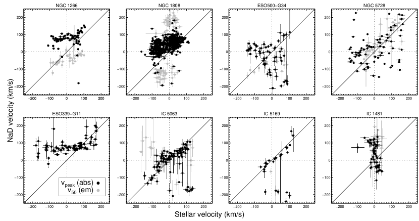
Figure 10: Na I D velocity ($v_{\mathrm{peak}}$) vs. stellar velocity. Na I D emission and absorption lines are shown as black circles and gray crosses, and error bars are 1$\sigma$. Black solid lines of equality and dashed zero-velocity lines are overplotted. Clear deviations from stellar rotation are evident in every case.

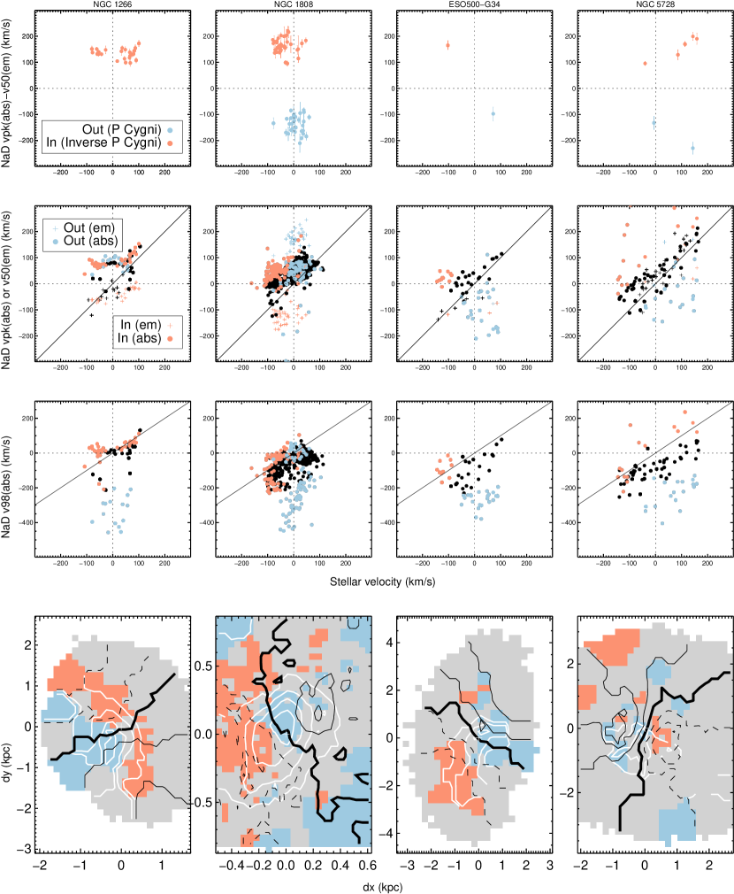
Figure 11: (Top row) Velocity difference between Na I D absorption and emission lines in each Voronoi bin vs. stellar velocity. P-Cygni profiles suggesting outflow are negative velocity differences and shown in blue; inverse P-Cygni profiles are positive and red. 1$\sigma$ errors in velocity difference are shown. (Second row) Peak or central Na I D velocity vs. stellar velocity. Crosses (circles) represent Na I D emission (absorption). Black symbols show bins that do not meet one of the criteria for inflow or outflow. Blue (red) symbols show data that meet one of the criteria for outflow (inflow); see Section 4. (Third row) Maximum Na I D absorption velocity vs. stellar velocity. (Bottom row) Maps of outflow and inflow. Gray shaded regions contain data but no detection of outflow or inflow. colour shaded regions are as described above. Black contours show stellar velocity; the solid thick contour locates $v=0$ km s^-1, and the other contours are labeled in Fig. 1. White contours show $W_{\mathrm{eq}}^{\mathrm{abs}}$; labels are in Å.

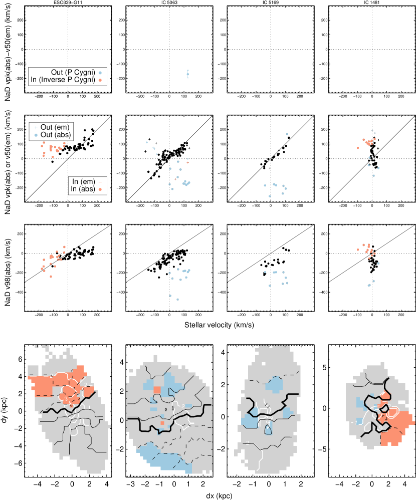
Figure 11: Continued.

We use two methods to trace these discrepant motions. The first is by measuring significant velocity differences between Na I D absorption and emission lines (i.e., P Cygni or inverse P Cygni profiles) in each Voronoi bin. This is a typical method for outflow and inflow detection in Na I D and other resonance lines. The second is to look for significant deviations of either Na I D absorption or emission from stellar motion. We use as a reference in each Voronoi bin the stellar velocity in that bin. We rely throughout on the expectation from observations (Phillips, 1993), simple models (Rubin et al., 2011; Roberts-Borsani & Saintonge, 2019), and radiative transfer calculations (Prochaska et al., 2011) that resonance absorption arises on the near side of a flow (thus showing a redshift during inflow and a blueshift during outflow) while resonance emission arises on the far side of a flow (thus showing a blueshift during inflow and a redshift during outflow). We display these velocity differences for each galaxy in the first three rows of Fig. 11.

In the first method, that of P Cygni or inverse P Cygni detection, we require a 2$\sigma$ detection of $v_{\mathrm{abs}}-v_{\mathrm{em}}<0$ for outflow or $v_{\mathrm{abs}}-v_{\mathrm{em}}>0$ for inflow. In practice, almost all of these detections have $|v_{\mathrm{abs}}-v_{\mathrm{em}}|>100$ km s^-1. Smaller offsets would make the emission and absorption blend into each other. It is possible that blending of these profiles in fact overestimates the velocity offset of these lines in integrated spectra (Prochaska et al., 2011). For these resolved data, however, emission and absorption resulting from physically distinct locations in an inflow or outflow are expected to have different kinematics, as we discuss above.

In the second method, we require the Na I D velocity in absorption or emission to differ from the stellar reference velocity by a significant amount. We choose the conservative criteria that the velocities differ from stellar in each Voronoi bin by at least 100 km s^-1 (e.g., twice the threshold in Rupke et al. 2005b) and differ from the stellar reference velocity by at least 2$\sigma$. The first criterion means a bin contains inflowing gas when $v_{\mathrm{50\%,em}}-v_{\star}<-100$ km s^-1 (blueshifted emission) or $v_{\mathrm{50\%,abs}}-v_{\star}>100$ km s^-1 (redshifted absorption) and it contains outflowing gas when $v_{\mathrm{50\%,em}}-v_{\star}>100$ km s^-1 (redshifted emission) or $v_{\mathrm{50\%,abs}}-v_{\star}<-100$ km s^-1 (blueshifted absorption). The 100 km s^-1 threshold may filter out deviations due to radial streaming motions along spiral arms (e.g., Shetty et al., 2007) or bars (Regan et al., 1999) or due to tidal motions that appear in merging systems (e.g., Rupke & Veilleux, 2013). We also allow an outflow detection if the absorption line wing is highly blueshifted ($v_{\mathrm{98\%,abs}}-v_{\star}<-200$ km s^-1), which is a robust quantity for defining outflow in starburst galaxies (e.g., Rupke & Veilleux, 2013).

These methods are largely consistent with each other; i.e., an inflow or outflow detected with the first method is typically also an outflow as defined using the second method. Examples where the methods diverge are NGC 5728, in which we observe a few apparently inflowing inverse P Cygni profiles for which the emission component is near the stellar velocity, and NGC 1808, in which we observe P Cygni profiles for which the absorption component is near the stellar velocity. In the case of NGC 1808, this is a consequence of absorption tracing the foreground disk in places where the emission traces the outflow (Phillips, 1993); the reverse could be true in NGC 5728.

We detect inflow and/or outflow in every galaxy in our sample over projected areas that are 10–40% of the stellar disk visible in the FOV, as shown in the bottom row of Fig. 11 and in Table 6. These correspond to physical areas of 1–18 kpc². We detect outflow in 7/8 systems, and inflow in 7/8 systems.

In 4/7 systems with an outflow (NGC 1266, NGC 1808, ESO 500$-$G34, IC 5169), neutral gas motions are consistent with the picture of a minor-axis flow, roughly oriented along the stellar zero-velocity contour. Two of these, NGC 1266 and NGC 1808, have prior minor-axis outflow detections in Na I D (Davis et al., 2012; Phillips, 1993). These four have the highest disk inclinations among the Na I D outflow detections.

Of the other 3/7 systems with an outflow, IC 5063 has a known radio jet that is accelerating ionized, neutral, and molecular gas along the major axis (Morganti et al., 1998, 2007, 2015). The outflowing gas we detect in Na I D is likely the dusty counterpart. In NGC 5728, there is a known ionized, minor-axis outflow (Durré & Mould, 2019; Shin et al., 2019; Shimizu et al., 2019) that is blueshifted in the NW and redshifted in the SE (corresponding to the bottom and top of our IFS maps). Some of the motions we observe may be connected with this narrow line region outflow, but not all Voronoi bins with detected outflow are consistent with this orientation. Finally, IC 1481 has an irregular morphology, low inclination, and twisted stellar isovelocity contours. Thus, determining the minor axis is difficult and the relationship between the gas kinematics and galaxy structure is unclear.

The inflow signatures we observe are spatially coherent in most cases. While the relationship between these regions and the underlying galaxy structure is not obvious in every galaxy, the inflow often lies closer to the projected major axis than the minor axis of the system. In most of these cases, the spatial footprint of the inflowing gas is largely confined to one side of the disk, with the exceptions of NGC 1266 and NGC 5728. 4/7 of the systems with inflows contain bars, and all are spirals.

Na I D emission is present in almost every galaxy in the sample, and P Cyngi or inverse P Cygni profiles show up in 5/8 systems. P Cygni profiles (blueshifted absorption and redshifted emission) are observed in spatially-resolved observations of galactic outflows in a few nearby galaxies (Phillips, 1993; Rupke & Veilleux, 2015; Perna et al., 2019; Baron et al., 2020), as well as others at high redshift (Rubin et al., 2011; Martin et al., 2013; Bordoloi et al., 2016), and are a result of radiation transfer effects in the outflow (Prochaska et al., 2011). However, to our knowledge, this is the first detection of inverse P Cygni profiles across galactic disks.

Besides the orientation of the flows, the other properties of the outflowing and inflowing gas are remarkably similar. As shown in Table 6, both flows typically extend to 50–75% of the edge of the stellar disk detected by WiFeS, as seen by comparing the maximum observed radii of the disk $R_{\mathrm{max}}^{\mathrm{disk}}$ to the maximum observed inflow and outflow radii, $R_{\mathrm{max}}^{\mathrm{out}}$ and $R_{\mathrm{max}}^{\mathrm{out}}$. The maximum inflow and outflow radii range from 1 to 6 kpc. They also are projected onto a similar areal percentage of the stellar disk, up to 25% (median 18% for inflows and 12% for outflows). The higher median value for the inflows may reflect the tendency for these flows to be closer to the major axis than to the minor axis.

There are not systematic differences across the sample in log($N($Na I$)$/cm^-2) or $W_{\mathrm{eq}}$ between the inflow and outflow regions. The area-weighted average and standard deviation of log($N($Na I$)$/cm^-2) are (13.6$\pm$0.6) and (13.5$\pm$0.6) for inflow and outflow, respectively. For $W_{\mathrm{eq}}$, the average and standard deviation are (1.9$\pm$1.8) Å and (1.6$\pm$2.9) for inflow and outflow. The luminosity- and area-weighted statistics are comparable.

Table 6: Projected radii and areas, as displayed in the bottom row of Fig. 11. Listed are the projected maximum radius of the disk $R_{\mathrm{max}}^{\mathrm{disk}}$, inflow $R_{\mathrm{max}}^{\mathrm{in}}$, and outflow $R_{\mathrm{max}}^{\mathrm{out}}$; the projected disk area $A^{\mathrm{disk}}$; and the percent of projected disk area classified as showing inflow, $A^{\mathrm{in}}$, or outflow, $A^{\mathrm{out}}$.

Galaxy	$R_{\mathrm{max}}^{\mathrm{disk}}$	$R_{\mathrm{max}}^{\mathrm{in}}$	$R_{\mathrm{max}}^{\mathrm{out}}$	$A^{\mathrm{disk}}$	$A^{\mathrm{in}}$	$A^{\mathrm{out}}$
—	kpc	kpc	kpc	kpc2	%	%
NGC 1266	2.54	2.14	1.97	13.45	25	17
NGC 1808	1.04	0.86	1.04	1.94	18	25
ESO500-G34	4.54	3.29	2.65	36.14	13	12
NGC 5728	4.04	3.18	3.72	30.16	7	9
ESO339-G11	8.53	6.24	0.00	85.89	20	0
IC 5063	4.56	3.22	3.74	39.29	1	17
IC 5169	4.55	0.00	2.49	25.38	0	10
IC 1481	5.59	5.44	2.50	62.84	24	4

5 DISCUSSION

We have detected ubiquitous and spatially-extended flows of cool, neutral gas across our S7 subsample that differ significantly from stellar motion. The correlations between gas and dust properties point to the dusty nature of these flows. We have characterized these correlations within individual galaxies and within the sample as a whole to compare to previous results and to benchmark future, larger integral-field studies of external galaxies.

The correlations between $N$(Na I D) or $W_{\mathrm{eq}}$ and $E(B-V)$ have not been extensively characterized in external galaxies, particularly at the spatially-resolved level. Thus our subsample, despite its modest size in terms of number of galaxies, represents a significant addition. The relevant observables have for decades been used to characterize the Milky Way’s ISM, so connecting these data to other galaxies is an important step.

In particular, we show that the relationship between $W_{\mathrm{eq}}$ and various dust measures is not the same from galaxy to galaxy (Fig. 3–5). The correlation between $W_{\mathrm{eq}}$ and measures of colour excess probably reflects a 3D spatial connection between neutral gas and dust. However, $W_{\mathrm{eq}}$ and $E(B-V)$ are indirect measures of the amount of gas and dust along a given line of sight. In these data, absorption lines dominate total $W_{\mathrm{eq}}$ in most spaxels, with resonant line emission biased toward low-$E(B-V)$ sightlines. Absorption-line $W_{\mathrm{eq}}$ is directly connected to column density (the curve of growth), but it is modulated by covering factor. A high $N$(Na I) line of sight with low $C_{f}$ can have the same $W_{\mathrm{eq}}$ as a line with low $N$(Na I) and high $C_{f}$. $N$(Na I) is in turn dependent on optical depth and linewidth.

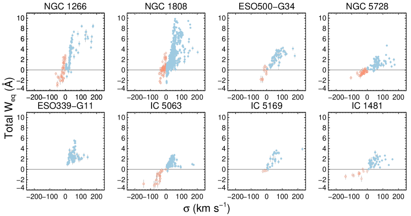
Figure 12: Total fitted Na I D equivalent width vs. velocity dispersion in each component. Spaxels with more than one component are represented by multiple points. Absorption components are shown in light blue with positive $\sigma$; emission components are shown in light red with negative $\sigma$. The median and standard deviation of correlation coefficients are 0.6$\pm$0.2 for absorption and 0.7$\pm$0.2 for emission. This illustrates that $\sigma$ is one of the primary parameters modulating equivalent width.

Based on nuclear galaxy spectra, Heckman et al. (2000) find that the depth of the Na I D profile (which they suggest depends primarily on $C_{f}$) is correlated with stellar colour and colour excess from gas measurements. They argued that increasing dust obscuration is thus directly connected to the increasing covering factor of the neutral gas. However, we do not find that equivalent width correlates strongly with either $\tau$ or $C_{f}$. The linear Pearson correlation coefficients of $W_{\mathrm{eq}}^{\mathrm{abs}}$ with $C_{f}$ and $\tau$ are $-0.1\pm 0.3$ and $0.2\pm 0.3$ (median plus or minus standard deviation). Instead, we find that total $W_{\mathrm{eq}}$ increases with increasing absorption linewidth and decreases with increasing emission linewidth in most systems (Fig. 12). The linear Pearson correlation coefficients of $W_{\mathrm{eq}}$ with $\sigma_{\mathrm{abs}}$ and $\sigma_{\mathrm{em}}$ are $0.6\pm 0.2$ and $-0.7\pm 0.2$. Thus, equivalent width, colour excess produced by dust, and total line dispersion are intimately correlated. If the correct picture is the collection of compact clouds discussed above (Section 3; Werk et al. 2019; Peek & Clark 2019), then these quantities may each scale with the number of clouds along the line of sight.

Considering all of the points within our sample, gas and dust correlations extend relationships determined from lower-$E(B-V)$ sightlines within the Milky Way and some external sightlines. In $N$(Na I D) vs. $E(B-V)$ space, they straddle correlations from Hobbs (1974) and Phillips et al. (2013) and lie in the same space as high-$E(B-V)$ infrared luminous galaxies. In $W_{\mathrm{eq}}$ vs. $E(B-V)$ space, they are on average very consistent with relationships from low-$z$ star-forming galaxies. They also largely lie within the envelope of previous single-sightline observations of infrared-luminous and star-forming galaxies at high $E(B-V)$ (Rupke et al., 2005a, 2008; Chen et al., 2010), though with more scatter to lower $W_{\mathrm{eq}}$ due to the sensitivity of our data. This in turn suggests that the dusty, neutral gas in these flows likely has similar physical conditions to gas in the disks and halos of the Milky Way and nearby star-forming galaxies. These similarities have been used to, e.g., calculate H I column densities from Na I D properties (e.g., Rupke et al., 2005a). Thus, our results lend strength to the H I column densities estimated in this way, despite the uncertainties due to ionization state and dust depletion. The mass outflow rates computed for neutral outflows—which are critical for evaluating their role as negative feedback in galaxy evolution—in turn depend on these column density estimates (e.g., Rupke et al., 2005b).

We do not claim that this sample is at all representative, either of the S7 sample as a whole or of local galaxies more generally. In particular, the subsample has been selected for its strong Na I D signatures. However, it is well-suited for characterizing the Na I D feature and its connection to dust, as well as illustrating how it can be used to detect both outflows and inflows. We also note that the signatures of these phenomena are widely-distributed across the disks of these systems and would not be well-characterized by single-aperture spectra. Thus integral-field studies of these flows, though their sample sizes are inherently limited, are critical to determining their properties and impact.

The detection of inverse P Cygni profiles in Na I D in half of these data cubes is potentially a first for external galaxy sightlines. In several of these data cubes, the signature is seen in a large number of spaxels. Sensitive, spatially-resolved observations help to uncover these, since the nuclear spectra tend to be dominated by absorption or outflow. Higher spectral resolution is key, as well ($R=7000$ at Na I D for WiFeS), since the linewidths in spaxels showing these inverse P Cygni profiles are narrow (Fig. 2) and the velocity shifts are not large ($\la$200 km s^-1; Fig. 11). Previous single-aperture studies like those with the SDSS ($R\sim 2000$ at Na I D) significantly smear and weaken these signatures, making them more difficult to interpret. Finally, moderate-resolution spectral templates (Valdes et al., 2004) yield high-quality subtraction of the stellar continuum.

Inverse P Cygni profiles in Na I D are seen in spectra of T Tauri and Herbig Ae stars (Edwards et al., 1994; Grinin et al., 1994), in which the signature is interpreted as accretion. The picture sketched by Roberts-Borsani & Saintonge (2019) in which inverse P Cygni profiles should appear in lines of sight through high-inclination disks due to infall appears to apply here. The inflow signatures we observe prefer the projected major axis and 7/8 of our disks have $i>50^{\circ}$. Presumably the same radiation transfer effects that arise in the outflow and produce P Cygni profiles can produce their inverse. Radiative transfer simulations, like those in Prochaska et al. (2011), could test this postulate.

Despite the selection bias, the frequent detection of radial motions consistent with outflow and inflow is striking. Our results are thus of a piece with the ubiquity of both inflow and outflow signatures in nearby AGN from single-aperture studies (Krug et al., 2010; Roberts-Borsani & Saintonge, 2019; Nedelchev et al., 2019). Single-aperture studies have also found that inflow dominates in edge-on systems and outflow in face-on systems (e.g., Chen et al., 2010; Roberts-Borsani & Saintonge, 2019). A similar result in our spatially-resolved study is the alignment of outflow signatures along the minor axis and the signatures of inflow that lie closer to the projected major axis. We find both signatures in many cases, rather than inflow or outflow dominating, despite 7/8 galaxies having inclination $i>50^{\circ}$.

While the disks in these galaxies may collimate an inner wind regardless of the power source, we note that NGC 5728 (Durré & Mould, 2018), IC 5063 (Morganti et al., 2007), and possibly NGC 1266 (Nyland et al., 2013) contain small-scale radio jets. In NGC 5728 (and perhaps NGC 1266), this jet is oriented roughly along the projected minor axis, but in IC 5063 it is oriented along the projected major axis. In IC 5063, we observe that the outflowing neutral gas also preferentially lies along the major axis (Fig. 11).

The inflows we observe can be caused by gravitational effects in the disks themselves, such as bars, spiral arms, or other non-axisymmetric structures. We choose a conservative criterion for defining inflow that may preclude these possibilities in some cases, but we cannot rule them out. NGC 1808 has radial streaming motions that are reflected in ionized and molecular gas (Salak et al., 2016; Busch et al., 2017). It also has a steeper gas rotation curve than the stars. The molecular gas in IC 5063 shows a steep rotation curve, as well (Morganti et al., 2015). Finally, NGC 5728 hosts a stellar bar, nuclear star-forming ring, and spiral arms, all of which produce gas dynamics different from the stars (Shimizu et al., 2019).

Undoubtedly there is some contribution from non-axisymmetric potentials to the neutral gas motions we observe. Tidal motions may also contribute in, e.g., IC 1481. However, the magnitudes of the discrepant ionized and molecular gas motions in NGC 1808, IC 5063, and NGC 5728 (of the order $\sim$100 km s^-1 or less compared to stellar rotation) are below our detection threshold if these motions were also present in neutral gas traced by Na I D. Furthermore, if we choose the ionized gas $v_{50\%}$ or the velocity at peak flux in place of stellar velocity as a reference point, we find even more widespread detection of inflow and outflow in these systems. These suggest that the motions we observe may not be dominated by inflow due to secular disk structures.

A plausible alternative is that the dusty inflows we observe at projected radii $<$10 kpc are the endpoint of inflows of cold, circumgalactic gas. Co-rotating gas is observed in Mg II absorption in extended galactic disks at a substantial fraction of the virial radius (i.e., well into the halo or circumgalactic medium; Ho et al. 2017; Zabl et al. 2019). This gas may be radially inflowing at modest velocities ($\la$60 km s^-1; Ho et al. 2019). The inflow velocities we observe are typically higher at 100–200 km s^-1, though we intentionally exclude some inflowing gas at lower velocities and are limited in sensitivity to very low-velocity gas. This high-velocity gas could represent an acceleration of these circumgalactic inflows at small radius as the gas falls down the gravitational well.

6 SUMMARY

Our understanding of dusty, neutral flows in galaxies is increasingly being informed by integral-field spectroscopy of external galaxies. We here present a new analysis of eight data cubes from the S7 survey, a large IFS survey of nearby Seyfert galaxies in the Southern hemisphere. Uniquely, these data sensitively cover a wide field of view at a relatively high spectral resolution for galaxy surveys ($R=7000$ at Na I D). These galaxies were selected for their widespread Na I D signatures, including both resonant emission and absorption.

These data enable us to characterize the spatially-resolved relationship between the cool, neutral gas (as traced by Na I D) and dust columns (as traced by stellar and gas $E(B-V)$) in these systems. While this relationship has been studied extensively in the Milky Way, it is relatively unconstrained in external galaxy sightlines and detailed spatially-resolved studies exist for only a few galaxies. We find that these eight disks are consistent with previous measurements and extrapolations at $E(B-V)\sim 1$, though the range of $W_{\mathrm{eq}}^{\mathrm{abs}}$ and $N$(Na I D) traced by individual spatial locations is much larger, particularly in $W_{\mathrm{eq}}^{\mathrm{abs}}$. Milky Way measurements of Na I D and H I have been used to estimate the mass and energetics of galactic winds from Na I D only (e.g., Rupke et al., 2005a). The consistency we measure among Milky Way and external galaxy measurements of Na I D, $W_{\mathrm{eq}}$, and $E(B-V)$ lends credence to these estimates.

Within individual galaxies, strong and significant correlations exist between total $W_{\mathrm{eq}}$ and $E(B-V)$_⋆, $E(B-V)$_gas, and/or optical colour $g-i$. The correlations of $W_{\mathrm{eq}}$ with $g-i$ and $E(B-V)$_⋆ are the strongest. The parameters of linear regressions are on average consistent with physical expectations for $E(B-V)$_⋆/$E(B-V)$_gas and for intrinsic unattenuated colours. However, the linear slopes vary from galaxy to galaxy, and in half of the sample the three dust measures show some differences in how they relate to $W_{\mathrm{eq}}$. We find that equivalent width differences within a galaxy are largely driven by velocity dispersion. If compact clouds with small dispersion make up the cool ISM of these galaxies, then the correlations between Na I D and colour excess may reflect a changing number of clouds along the line of sight.

Using Doppler shifts of both resonant emission and absorption, we find spatially coherent signatures of high-velocity non-rotational flows ($|v_{\mathrm{abs}}-v_{\mathrm{em}}|>100$ km s^-1 and/or $|v_{\mathrm{abs/em}}-v_{\star}|>100$ km s^-1) in each of these high-inclination galaxy disks (7/8 have $i>50^{\circ}$). Outflow is observed in both blueshifted absorption or redshifted emission (or perhaps both; a P Cygni profile), while inflow is observed in redshifted absorption or blueshifted emission (or both; an inverse P Cygni profile). This is consistent with recent work on large, single-aperture surveys of nearby AGN (Krug et al., 2010; Roberts-Borsani & Saintonge, 2019; Nedelchev et al., 2019). We find that the column density, equivalent width, size, and area subtended by the inflows and outflows are not substantially different on average. The outflows are consistent with minor-axis collimation and/or jet driving, while the inflows are more closely aligned with the major axes. While some of the inflow motions may reflect tidal motions or secular streaming motions due to, e.g., bar or spiral arm potentials, their relatively high velocities could also point to other mechanisms such as the endpoints of halo-scale accretion.

For perhaps the first time in external galaxies, we detect ubiquitous inverse P Cygni profiles in Na I D, which is enabled by the relatively high spectral resolution of the data and spectral libraries of correspondingly high resolution. Profiles like this are found in accreting Galactic T Tauri and Herbig Ae stars (Edwards et al., 1994; Grinin et al., 1994), and in these cases are presumably due to infall onto galactic disks (Roberts-Borsani & Saintonge, 2019).

Ongoing and future IFS surveys like MaNGA and the Hector Galaxy Survey will probe these relationships over much larger sample sizes. The present sample exemplifies the importance of IFS for probing the nature of neutral gas flows in external galaxies, suggesting that these IFS surveys are necessary for improving on single-aperture studies of the cool, neutral medium. The current sample thus serves as a bridge between studies of the Milky Way and these larger IFS surveys, which will be able to better characterize the full parameter space of Na I D strength and dust column and galaxy type.

DATA AVAILABILITY

The data underlying this paper, and fits to the data, are available online at https://cloudstor.aarnet.edu.au/plus/s/zyE9jAjHWcGb12v or https://docs.datacentral.org.au/s7/. Spectral fitting software used in the paper is available at https://github.com/drupke/ifsfit.

SUPPORTING INFORMATION

Additional Supporting Information may be found in the online version of this article:

Figure 1. Images and maps of stellar and gas properties of each galaxy.

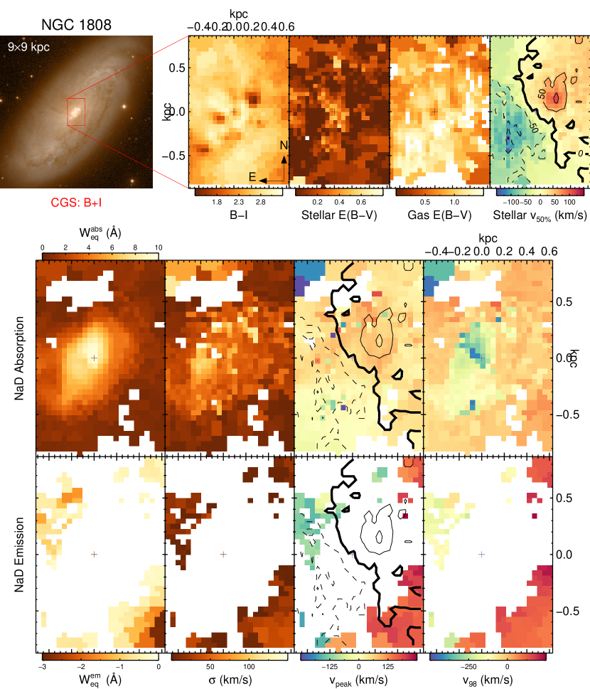
Figure 1: Continued.

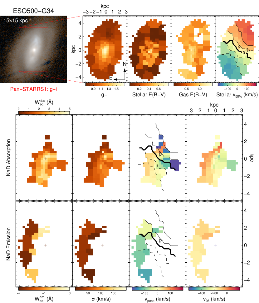
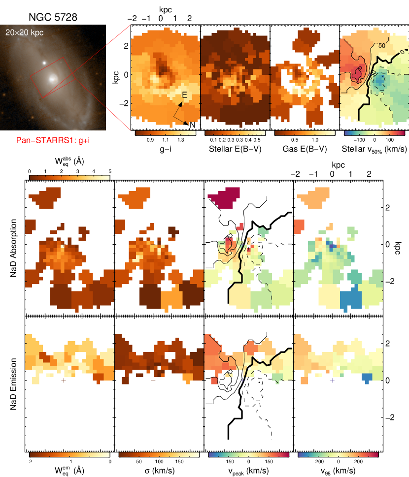
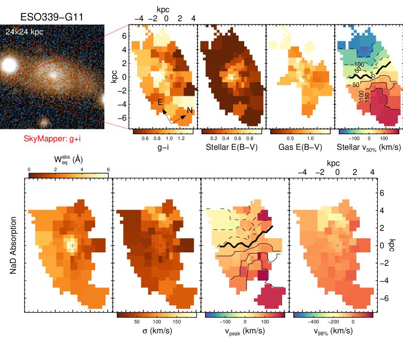
Figure 1: Continued.

Figure 1: Continued.

Figure 1: Continued.

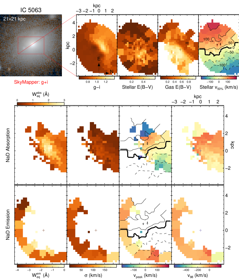
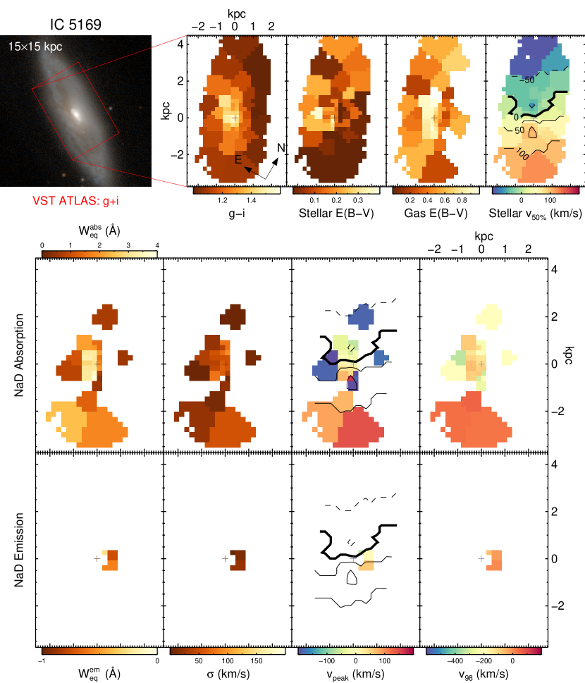
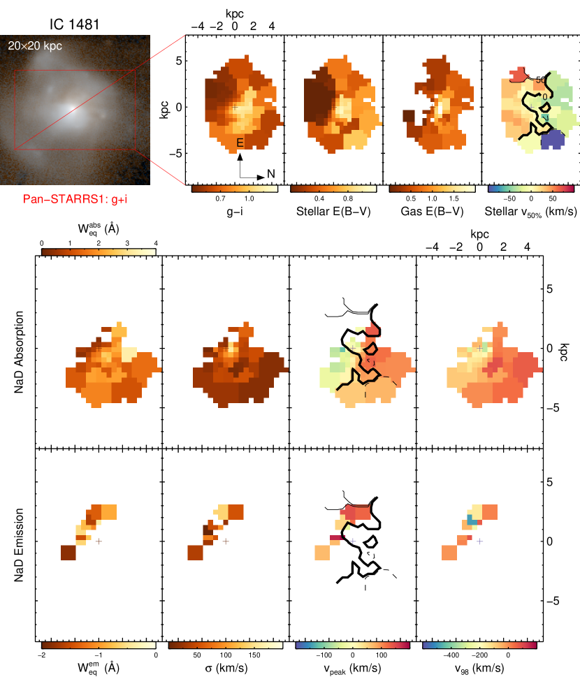
Figure 1: Continued.

Figure 1: Continued.

Figure 1: Continued.

Figure A1. Na I D absorption equivalent width vs. colour excess of the ionized gas in each galaxy, compared to MW and other external galaxy sightlines. The lines are as described in Fig. 6. Error bars are 1$\sigma$.

Figure A2. Na I D absorption column density vs. colour excess of the ionized gas in each galaxy, compared to MW and other external galaxy sightlines. The lines are as described in Fig. 7. Black filled (red open) circles represent two-component (one-component) fits. Lower limits are shown as small arrows.

Please note: Oxford University Press are not responsible for the content or functionality of any supporting materials supplied by the authors. Any queries (other than missing material) should be directed to the corresponding author for the paper.

Appendix A Column density and equivalent width vs. colour excess for individual galaxies

In Section 3, we combine measurements from individual galaxies to study $N$(Na I) and $W_{\mathrm{eq}}^{\mathrm{abs}}$ vs. gas $E(B-V)$. Plots for individual galaxies are available online.

References

- Balmaverde et al. (2019) Balmaverde B., et al., 2019, A&A, 632, A124
- Baron et al. (2016) Baron D., Stern J., Poznanski D., Netzer H., 2016, ApJ, 832, 8
- Baron et al. (2020) Baron D., Netzer H., Davies R. I., Xavier Prochaska J., 2020, MNRAS, 494, 5396
- Bedregal et al. (2006) Bedregal A. G., Aragón-Salamanca A., Merrifield M. R., 2006, MNRAS, 373, 1125
- Beifiori et al. (2011) Beifiori A., Maraston C., Thomas D., Johansson J., 2011, A&A, 531, A109
- Bordoloi et al. (2016) Bordoloi R., Rigby J. R., Tumlinson J., Bayliss M. B., Sharon K., Gladders M. G., Wuyts E., 2016, MNRAS, 458, 1891
- Busch et al. (2017) Busch G., Eckart A., Valencia-S. M., Fazeli N., Scharwächter J., Combes F., García-Burillo S., 2017, A&A, 598, A55
- Calzetti et al. (2000) Calzetti D., Armus L., Bohlin R. C., Kinney A. L., Koornneef J., Storchi-Bergmann T., 2000, ApJ, 533, 682
- Capetti et al. (1996) Capetti A., Axon D. J., Macchetto F., Sparks W. B., Boksenberg A., 1996, ApJ, 466, 169
- Cappellari (2012) Cappellari M., 2012, pPXF: Penalized Pixel-Fitting stellar kinematics extraction (ascl:1210.002)
- Cappellari & Copin (2003) Cappellari M., Copin Y., 2003, MNRAS, 342, 345
- Cappellari & Copin (2012) Cappellari M., Copin Y., 2012, Voronoi binning method (ascl:1211.006)
- Cappellari & Emsellem (2004) Cappellari M., Emsellem E., 2004, PASP, 116, 138
- Cappellari et al. (2011) Cappellari M., et al., 2011, MNRAS, 413, 813
- Chen et al. (2010) Chen Y.-M., Tremonti C. A., Heckman T. M., Kauffmann G., Weiner B. J., Brinchmann J., Wang J., 2010, AJ, 140, 445
- Childress et al. (2014a) Childress M., Vogt F., Nielsen J., Sharp R., 2014a, PyWiFeS: Wide Field Spectrograph data reduction pipeline (ascl:1402.034)
- Childress et al. (2014b) Childress M. J., Vogt F. P. A., Nielsen J., Sharp R. G., 2014b, Ap&SS, 349, 617
- Cicone et al. (2014) Cicone C., et al., 2014, A&A, 562, A21
- Concas et al. (2019) Concas A., Popesso P., Brusa M., Mainieri V., Thomas D., 2019, A&A, 622, A188
- Davis et al. (2012) Davis T. A., et al., 2012, MNRAS, 426, 1574
- Dopita et al. (2007) Dopita M., Hart J., McGregor P., Oates P., Bloxham G., Jones D., 2007, Ap&SS, 310, 255
- Dopita et al. (2010) Dopita M., et al., 2010, Ap&SS, 327, 245
- Dopita et al. (2015) Dopita M. A., et al., 2015, ApJS, 217, 12
- Durré & Mould (2018) Durré M., Mould J., 2018, ApJ, 867, 149
- Durré & Mould (2019) Durré M., Mould J., 2019, ApJ, 870, 37
- Edwards et al. (1994) Edwards S., Hartigan P., Ghandour L., Andrulis C., 1994, AJ, 108, 1056
- González Delgado et al. (2005) González Delgado R. M., Cerviño M., Martins L. P., Leitherer C., Hauschildt P. H., 2005, MNRAS, 357, 945
- Greener et al. (2020) Greener M. J., et al., 2020, MNRAS, 495, 2305
- Grinin et al. (1994) Grinin V. P., The P. S., de Winter D., Giampapa M., Rostopchina A. N., Tambovtseva L. V., van den Ancker M. E., 1994, A&A, 292, 165
- Heckman et al. (2000) Heckman T. M., Lehnert M. D., Strickland D. K., Armus L., 2000, ApJS, 129, 493
- Hewett et al. (2006) Hewett P. C., Warren S. J., Leggett S. K., Hodgkin S. T., 2006, MNRAS, 367, 454
- Ho et al. (2011) Ho L. C., Li Z.-Y., Barth A. J., Seigar M. S., Peng C. Y., 2011, ApJS, 197, 21
- Ho et al. (2017) Ho S. H., Martin C. L., Kacprzak G. G., Churchill C. W., 2017, ApJ, 835, 267
- Ho et al. (2019) Ho S. H., Martin C. L., Turner M. L., 2019, ApJ, 875, 54
- Hobbs (1974) Hobbs L. M., 1974, ApJ, 191, 381
- Hogg et al. (2010) Hogg D. W., Bovy J., Lang D., 2010, arXiv e-prints, p. arXiv:1008.4686
- Husemann et al. (2017) Husemann B., et al., 2017, The Messenger, 169, 42
- Jeong et al. (2013) Jeong H., Yi S. K., Kyeong J., Sarzi M., Sung E.-C., Oh K., 2013, ApJS, 208, 7
- Kelly (2007) Kelly B. C., 2007, ApJ, 665, 1489
- Kewley et al. (2006) Kewley L. J., Groves B., Kauffmann G., Heckman T., 2006, MNRAS, 372, 961
- Krajnović et al. (2011) Krajnović D., et al., 2011, MNRAS, 414, 2923
- Kreckel et al. (2013) Kreckel K., et al., 2013, ApJ, 771, 62
- Krug et al. (2010) Krug H. B., Rupke D. S. N., Veilleux S., 2010, ApJ, 708, 1145
- Lamastra et al. (2009) Lamastra A., Bianchi S., Matt G., Perola G. C., Barcons X., Carrera F. J., 2009, A&A, 504, 73
- Landsman (1993) Landsman W. B., 1993, in Hanisch R. J., Brissenden R. J. V., Barnes J., eds, Astronomical Society of the Pacific Conference Series Vol. 52, Astronomical Data Analysis Software and Systems II. p. 246
- Lutz et al. (2020) Lutz D., et al., 2020, A&A, 633, A134
- Markwardt (2009) Markwardt C. B., 2009, in Bohlender D. A., Durand D., Dowler P., eds, Astronomical Society of the Pacific Conference Series Vol. 411, Astronomical Data Analysis Software and Systems XVIII. p. 251 (arXiv:0902.2850)
- Martin (2005) Martin C. L., 2005, ApJ, 621, 227
- Martin et al. (2013) Martin C. L., Shapley A. E., Coil A. L., Kornei K. A., Murray N., Pancoast A., 2013, ApJ, 770, 41
- Morganti et al. (1998) Morganti R., Oosterloo T., Tsvetanov Z., 1998, AJ, 115, 915
- Morganti et al. (2007) Morganti R., Holt J., Saripalli L., Oosterloo T. A., Tadhunter C. N., 2007, A&A, 476, 735
- Morganti et al. (2015) Morganti R., Oosterloo T., Oonk J. B. R., Frieswijk W., Tadhunter C., 2015, A&A, 580, A1
- Munari & Zwitter (1997) Munari U., Zwitter T., 1997, A&A, 318, 269
- Murga et al. (2015) Murga M., Zhu G., Ménard B., Lan T.-W., 2015, MNRAS, 452, 511
- Nedelchev et al. (2019) Nedelchev B., Sarzi M., Kaviraj S., 2019, MNRAS, 486, 1608
- Nyland et al. (2013) Nyland K., et al., 2013, ApJ, 779, 173
- Ott (2012) Ott T., 2012, QFitsView: FITS file viewer (ascl:1210.019)
- Peek & Clark (2019) Peek J. E. G., Clark S. E., 2019, ApJ, 886, L13
- Perna et al. (2017) Perna M., Lanzuisi G., Brusa M., Mignoli M., Cresci G., 2017, A&A, 603, A99
- Perna et al. (2019) Perna M., Cresci G., Brusa M., Lanzuisi G., Concas A., Mainieri V., Mannucci F., Marconi A., 2019, A&A, 623, A171
- Phillips (1993) Phillips A. C., 1993, AJ, 105, 486
- Phillips et al. (2013) Phillips M. M., et al., 2013, ApJ, 779, 38
- Poznanski et al. (2012) Poznanski D., Prochaska J. X., Bloom J. S., 2012, MNRAS, 426, 1465
- Prochaska et al. (2011) Prochaska J. X., Kasen D., Rubin K., 2011, ApJ, 734, 24
- Regan et al. (1999) Regan M. W., Sheth K., Vogel S. N., 1999, ApJ, 526, 97
- Richmond et al. (1994) Richmond M. W., Treffers R. R., Filippenko A. V., Paik Y., Leibundgut B., Schulman E., Cox C. V., 1994, AJ, 107, 1022
- Roberts-Borsani & Saintonge (2019) Roberts-Borsani G. W., Saintonge A., 2019, MNRAS, 482, 4111
- Roberts-Borsani et al. (2020) Roberts-Borsani G. W., Saintonge A., Masters K. L., Stark D. V., 2020, MNRAS, 493, 3081
- Rubin et al. (2011) Rubin K. H. R., Prochaska J. X., Ménard B., Murray N., Kasen D., Koo D. C., Phillips A. C., 2011, ApJ, 728, 55
- Rupke (2014a) Rupke D. S. N., 2014a, IFSRED: Data Reduction for Integral Field Spectrographs (ascl:1409.004)
- Rupke (2014b) Rupke D. S. N., 2014b, IFSFIT: Spectral Fitting for Integral Field Spectrographs (ascl:1409.005)
- Rupke & Veilleux (2011) Rupke D. S. N., Veilleux S., 2011, ApJ, 729, L27
- Rupke & Veilleux (2013) Rupke D. S. N., Veilleux S., 2013, ApJ, 768, 75
- Rupke & Veilleux (2015) Rupke D. S. N., Veilleux S., 2015, ApJ, 801, 126
- Rupke et al. (2005a) Rupke D. S., Veilleux S., Sanders D. B., 2005a, ApJS, 160, 87
- Rupke et al. (2005b) Rupke D. S., Veilleux S., Sanders D. B., 2005b, ApJS, 160, 115
- Rupke et al. (2005c) Rupke D. S., Veilleux S., Sanders D. B., 2005c, ApJ, 632, 751
- Rupke et al. (2008) Rupke D. S. N., Veilleux S., Baker A. J., 2008, ApJ, 674, 172
- Rupke et al. (2017) Rupke D. S. N., Gültekin K., Veilleux S., 2017, ApJ, 850, 40
- Salak et al. (2016) Salak D., Nakai N., Hatakeyama T., Miyamoto Y., 2016, ApJ, 823, 68
- Sánchez (2020) Sánchez S. F., 2020, ARA&A, 58, 99
- Sarzi et al. (2016) Sarzi M., Kaviraj S., Nedelchev B., Tiffany J., Shabala S. S., Deller A. T., Middelberg E., 2016, MNRAS, 456, L25
- Schlafly & Finkbeiner (2011) Schlafly E. F., Finkbeiner D. P., 2011, ApJ, 737, 103
- Sembach & Danks (1994) Sembach K. R., Danks A. C., 1994, A&A, 289, 539
- Sembach et al. (1993) Sembach K. R., Danks A. C., Savage B. D., 1993, A&AS, 100, 107
- Shanks et al. (2015) Shanks T., et al., 2015, MNRAS, 451, 4238
- Shastri et al. (2019) Shastri P., et al., 2019, in American Institute of Physics Conference Series. p. 090003, doi:10.1063/1.5110134
- Shetty et al. (2007) Shetty R., Vogel S. N., Ostriker E. C., Teuben P. J., 2007, ApJ, 665, 1138
- Shih & Rupke (2010) Shih H.-Y., Rupke D. S. N., 2010, ApJ, 724, 1430
- Shimizu et al. (2019) Shimizu T. T., et al., 2019, MNRAS, 490, 5860
- Shin et al. (2019) Shin J., Woo J.-H., Chung A., Baek J., Cho K., Kang D., Bae H.-J., 2019, ApJ, 881, 147
- Stumpff (1980) Stumpff P., 1980, A&AS, 41, 1
- Taylor et al. (2015) Taylor E. N., et al., 2015, MNRAS, 446, 2144
- Thomas et al. (2017) Thomas A. D., et al., 2017, ApJS, 232, 11
- Thomas et al. (2018) Thomas A. D., Dopita M. A., Kewley L. J., Groves B. A., Sutherland R. S., Hopkins A. M., Blanc G. A., 2018, ApJ, 856, 89
- Valdes et al. (2004) Valdes F., Gupta R., Rose J. A., Singh H. P., Bell D. J., 2004, ApJS, 152, 251
- Veilleux et al. (1995) Veilleux S., Kim D. C., Sanders D. B., Mazzarella J. M., Soifer B. T., 1995, ApJS, 98, 171
- Venturi et al. (2017) Venturi G., Marconi A., Mingozzi M., Carniani S., Cresci G., Risaliti G., Mannucci F., 2017, Frontiers in Astronomy and Space Sciences, 4, 46
- Véron-Cetty & Véron (2006) Véron-Cetty M. P., Véron P., 2006, A&A, 455, 773
- Véron-Cetty & Véron (2010) Véron-Cetty M. P., Véron P., 2010, A&A, 518, A10
- Viaene et al. (2017) Viaene S., Sarzi M., Baes M., Fritz J., Puerari I., 2017, MNRAS, 472, 1286
- Villar Martín et al. (2014) Villar Martín M., Emonts B., Humphrey A., Cabrera Lavers A., Binette L., 2014, MNRAS, 440, 3202
- Wakker & Mathis (2000) Wakker B. P., Mathis J. S., 2000, ApJ, 544, L107
- Welty & Hobbs (2001) Welty D. E., Hobbs L. M., 2001, ApJS, 133, 345
- Welty et al. (1994) Welty D. E., Hobbs L. M., Kulkarni V. P., 1994, ApJ, 436, 152
- Werk et al. (2019) Werk J. K., et al., 2019, ApJ, 887, 89
- Williams et al. (2010) Williams M. J., Bureau M., Cappellari M., 2010, MNRAS, 409, 1330
- Wolf et al. (2018) Wolf C., et al., 2018, Publ. Astron. Soc. Australia, 35, e010
- Zabl et al. (2019) Zabl J., et al., 2019, MNRAS, 485, 1961