The formation of the Milky Way halo and its dwarf satellites: a NLTE-1D abundance analysis.
IV. Segue 1, Triangulum ii, and Coma Berenices UFDs.

Abstract

We present atmospheric parameters and abundances for chemical elements from carbon to barium in metal-poor stars in Segue 1 (seven stars), Coma Berenices (three stars), and Triangulum ii (one star) ultra-faint dwarf galaxies (UFDs). The effective temperatures rely on new photometric observations in the visible and infra-red bands, obtained with the 2.5 m telescope of the SAI MSU Caucasian observatory. Abundances of up to fourteen chemical elements were derived under the non-local thermodynamic equilibrium (NLTE) line formation, and LTE abundances were obtained for up to five more elements. For the first time we present abundance of oxygen in Seg 1 S1 and S4, silicon in ComaBer S2 and Tri ii S40, potassium in Seg 1 S1$-$S6 and ComaBer S1$-$S3, and barium in Seg 1 S7. Three stars in Segue 1, two stars in Coma Berenices, and Triangulum ii star have very low [Na/Mg] of $-1.08$ to $-1.67$ dex, which is usually attributed in the literature to an odd-even effect produced by nucleosynthesis in massive metal-free stars. We interpret this chemical property as a footprint of first stars, which is not blurred due to a small number of nucleosynthesis events that contributed to chemical abundance patterns of the sample stars. Our NLTE abundances of Sr and Ba in Coma Berenices, Segue 1, and Triangulum ii report on lower [Sr/Ba] abundance ratio in the UFDs compared to that in classical dwarf spheroidal galaxies and the Milky Way halo. However, in UFDs, just as in massive galaxies, [Sr/Ba] is not constant and it can be higher than the pure r-process ratio. We suggest a hypothesis of Sr production in metal-poor binaries at the earliest epoch of galactic evolution.

1 Introduction

Ultra-faint dwarf galaxies (UFDs) are the least luminous, oldest, most dark matter-dominated, most metal-poor, and least chemically evolved stellar systems known (for a review, see Simon, 2019; Tolstoy et al., 2009). From analyses of colour-magnitude diagrams and spectra, it is known that some faint dwarf galaxies formed their stars within a short period, less than 1 Gyr (Okamoto et al., 2008, 2012; Frebel & Bromm, 2012; Frebel et al., 2014; Venn et al., 2017). Short star formation timescale together with a low stellar mass result in a small number of nucleosynthesis events that contributed to chemical composition of long-lived stars observed today in faint dwarf galaxies (see, for example, Frebel et al., 2014).

The observed abundance patterns in individual stars contain information about properties of nucleosynthesis events and their progenitors and the efficiency of gas mixing at the early epoch of galactic formation. The more enrichment events a system encounters, the more blurred the signature of an individual event becomes. Unusual chemical element abundance ratios found in some metal-poor stars are interpreted as evidence of individual nucleosynthesis episodes. Nearby dwarf galaxies are the best places to find such stars. For example, Koch et al. (2008) reported the chemical composition of two stars in the Hercules Dwarf Spheroidal Galaxy (dSph) with high ratio of hydrostatic to explosive $\alpha$-element abundance ratios, [Mg/Ca] = 0.94 and 0.58 dex and [O/Ca] = 1.25 and $<$ 0.70 dex, respectively. A similar chemical feature, [Mg/Ca] = 0.61, was found in S119 in Draco dSph (Fulbright et al., 2004). However, for this star, Shetrone et al. (1998) found a normal [Ca/Mg] ratio of 0.12. Hansen et al. (2020) found [Mg/Ca] = 0.3 in a star in Grus ii UFD. We note the large errors of 0.20 dex and 0.26 dex for Mg and Ca abundances, respectively, found by Hansen et al. (2020). In the Milky Way (MW) halo, there are stars with high [Mg/Ca] $>0.5$ (for example, Frebel et al., 2008; Norris et al., 2013; Keller et al., 2014; Depagne et al., 2002; Cohen et al., 2008). Thus, similar chemical abundance peculiarities could be found in stars in different galaxies.

Some dwarf galaxies may have individual endemic chemical peculiarities. For example, in Hor i UFD stars, Nagasawa et al. (2018) found surprisingly low [$\alpha$/Fe] $\simeq$ 0 in contrast to typical [$\alpha$/Fe] $\sim$ 0.3 found in the literature in the majority of metal-poor (MP) stars in the MW and dwarf galaxies. Ret ii, Tuc iii, and Gru ii UFDs are known for their stars enhanced in r-process elements (Ji et al., 2016b; Hansen et al., 2017, 2020) in contrast to the extremely low neutron-capture (n-capture) element abundances found in stars in other UFDs (see, for example, Mashonkina et al., 2017b; Ji et al., 2019).

There are stars with normal chemical composition in dwarf galaxies as well. For example, in Boo ii UFD, Koch & Rich (2014) and Ji et al. (2016c) found no chemical peculiarities and abundance patterns to be similar to the normal MW halo stars for all elements except low neutron-capture element abundances.

Chemical properties of stars in different galaxies depend on the formation history of their host galaxies. To understand how different or similar the first stars in different UFDs were and how well the gas in a given UFD was mixed, it is necessary to perform a careful homogeneous abundance determination in stars in different UFDs. In the present analysis, we selected stars in the smallest UFDs known to date with individual high-resolution spectra available in the archives. The selected UFDs, namely, Segue 1, Triangulum ii, and Coma Berenices meet the criteria of Frebel & Bromm (2012) and could be recognized as surviving first galaxies.

Segue 1 (Seg 1) with M_V = $-1.5$ and half-light radius r_1/2 = 30 pc (Martin et al., 2008; Geha et al., 2009; Simon et al., 2011) is one of the smallest and faintest known UFDs, that first was thought to be a globular cluster (Belokurov et al., 2007; Niederste-Ostholt et al., 2009). Using high-resolution spectra, Frebel et al. (2014, hereafter F14) and Norris et al. (2010, hereafter N10) determined the chemical composition of Segue 1 stars. Stars in Seg 1 span a wide metallicity range of $-3.78<$ [Fe/H] $<-1.42$ and show high [$\alpha$/Fe], indicating enrichment only from massive stars. This result is in line with medium resolution observations of Vargas et al. (2013, hereafter V13).

Triangulum ii (Tri ii) has M_V = $-1.8$ and r_1/2 = 34 pc (Laevens et al., 2015; Martin et al., 2016; Kirby et al., 2017), which is very similar to Seg 1. From low-resolution observations of 13 Tri ii members, Kirby et al. (2017, hereafter K17) found that their metallicities range from $-2.86$ to $-1.40$. The two brightest stars in Tri ii were studied with high-resolution spectra (Kirby et al., 2017; Venn et al., 2017; Ji et al., 2019). Tri ii S40 with [Fe/H] = $-2.9$ shows normal [$\alpha$/Fe] of 0.3, while low [Na/Fe] from $-1.1$ (Kirby et al., 2017) to $-0.8$ (Ji et al., 2019), high [K/Fe] of 0.8, and high [Ni/Fe] of 0.5. Another star, S46, with [Fe/H] $\simeq-2$ shows low [$\alpha$/Fe] $<0$. The quality of S46 observed spectrum does not enable iron-peak element abundances measurements to reconcile whether low [$\alpha$/Fe] is caused by a prompt type  ia supernova (SN) enrichment or the stochastic sampling of a few massive SNe ii (Venn et al., 2017; Ji et al., 2019). It is worth noting that S46 is likely not a member of Tri ii, since its membership probability p = 0.04 found by McConnachie & Venn (2020) is low.

Coma Berenices (ComaBer) has M_V = $-4.1$, r_1/2 = 70 pc (Belokurov et al., 2007; Martin et al., 2008), and is thus larger than Seg 1 and Tri ii. Chemical composition of the three brightest stars with V $\simeq$ 18 mag was determined by Frebel et al. (2010, hereafter F10) from analyses of high-resolution spectra. F10 found that the metallicity spans $-2.88$ $<$ [Fe/H] $<$ $-2.31$, and that the most metal-rich star shows slightly lower [$\alpha$/Fe] abundance ratio compared to more metal-poor stars. F10 concluded that more observations of stars with [Fe/H]$>-2$ are required to understand whether the higher iron abundance of this star could be due to an onset of iron production in SN ia or stochastic mixing of few massive SNe ii. V13 increased the statistics and determined [Fe/H] and [$\alpha$/Fe] of ten stars using medium resolution spectra. Stars in the V13 stellar sample have metallicities in the range $-3.38<$ [Fe/H] $<-2.12$ and various [$\alpha$/Fe] ratios: low [$\alpha$/Fe] $\simeq$ 0 in two stars with [Fe/H] $>-2.4$ and high [$\alpha$/Fe] $\simeq$ 0.3 to 0.9 dex in eight stars with [Fe/H] $<-2.4$. V13 concluded that low [$\alpha$/Fe] ratios in two stars with the highest [Fe/H] is caused by the production of iron in SN ia.

In this study, we revisit existing data on the stars in Segue 1, Triangulum ii, and Coma Berenices UFDs and determine accurate stellar parameters and chemical abundances, using new multiband photometric observations and accurate line formation calculations, taking into account deviations from the local thermodynamic equilibrium (LTE), i. e. using the NLTE approach.

This study is performed within a project on a homogeneous NLTE abundance analysis of stars in the Galactic dwarf satellites. The studies by Mashonkina et al. (2017a, hereafter M17a) and Mashonkina et al. (2017b, hereafter M17b), where accurate stellar parameters and the NLTE abundances were presented for 59 very metal-poor (VMP, $-4<$[Fe/H]$<-2$) stars in seven dwarf spheroidal galaxies (dSphs) and in the MW halo, gave rise to the project. Further, the stellar sample was complemented by Pakhomov et al. (2019, hereafter P19). This paper employs the same method of stellar parameter and the NLTE abundance determinations as in M17a, M17b, and P19.

Photometric observations and data reduction are described in Section 2. We outline the method of stellar parameter determination in Section 3. The derived stellar abundances and the methods are presented in Section 4. The discussion of the results and our conclusions are given in Sections 5 and 6, respectively.

2 Photometric observations and data reduction

Photometric observations were carried out with Moscow State University Sternberg Astronomical Institute (SAI MSU) Caucasian Mountain Observatory (CMO) 2.5 m telescope in February to April 2017, on nights with stable extinction, which was monitored by the astroclimate site monitor of CMO (Kornilov et al., 2014).

For observations in the BVRcIc bands, we used an NBI 4k x 4k camera produced by Niels Bohr Institute, Copenhagen. The preliminary reduction procedure comprises bias subtraction, nonlinearity and flat field correction. Magnitudes were derived with the source extractor package (Bertin & Arnouts, 1996) taking into account aperture corrections. Coordinates of the objects were derived with the astrometry package (Lang et al., 2010). Extinction measurements and photometric calibrations were made using the Landolt standards (Landolt & Clem, 2013), observed on the same nights. The equations of the transformation to the standard photometric system were derived earlier using Landolt standards (Clem & Landolt, 2013).

The $JHK$ photometric data were obtained with the ASTRONIRCAM camera (Nadjip et al., 2017) in dithering mode. Depending on the seeing and exposure time, 30 to 60 frames, 30 seconds each, were observed with each filter. Nonlinearity, dark current, and flat field corrections were taken into account. Photometry was carried out in the MKO system, with a further transformation to 2MASS according to equations from Leggett et al. (2006). GSPC P264-F star from the list of MKO photometric system standards (Leggett et al., 2006) was adopted as the main standard to which bright enough stars in the field were referred and served as reference stars for each investigated object. The derived magnitudes are listed in Table 1. An error of each magnitude is within several hundredths.

In addition to Coma Berenices and Segue 1 stars, we observed four stars investigated by Mashonkina et al. (2017a), namely three stars in Ursa Major ii (UMa ii) UFD and one star in Leo iv UFD, for which available literature infrared (IR) magnitudes are either of low accuracy or missing. In total, the observations in the infrared JHK bands were performed for ComBer S1–S3, Seg 1 S1–S3, UMa ii S1–S3, and Leo iv S1 stars, while the observations in the visible ($BVRcIc$) bands were performed only for three stars in Coma Berenices. For the remaining sample stars, the literature photometric data are accurate enough and were used for $T_{\rm eff}$ determination. For example, the errors in gri magnitudes for Seg 1 S1, S2, and S3 are within 0.011 dex, which translates in errors in $T_{\rm eff}$ smaller than 20 K for any of these stars, colour, and calibration.

Table 1: Photometric magnitudes obtained with the 2.5 ­m telescope of CMO of SAI MSU together with literature data.

Star	RA	DEC	$B$	$V$	$R_{c}$	$I_{c}$	$J$	$H$	$K$
Coma Berenices:
S1	12 26 43.44	+23 57 02.6	18.920	18.164	17.678	17.197	16.514 $\pm$ 0.010	15.996 $\pm$ 0.020	15.955 $\pm$ 0.020
S2	12 26 55.45	+23 56 09.5	18.854	18.099	17.608	17.115	16.407 $\pm$ 0.020	15.885 $\pm$ 0.030	15.834 $\pm$ 0.030
S3	12 26 56.66	+23 56 11.8	18.375	17.572	17.058	16.552	15.818 $\pm$ 0.020	15.272 $\pm$ 0.020	15.213 $\pm$ 0.020
Segue 1:
S1	10 07 10.07	+16 06 23.9		18.961			17.415 $\pm$ 0.009	16.931 $\pm$ 0.010	16.813 $\pm$ 0.013
S2	10 07 02.46	+15 50 55.2		18.221			16.691 $\pm$ 0.010	16.247 $\pm$ 0.013	16.136 $\pm$ 0.019
S3	10 07 42.71	+16 01 06.8		18.391			16.913 $\pm$ 0.017	16.451 $\pm$ 0.038	16.397 $\pm$ 0.017
S4	10 07 14.6	+16 01 54.5		18.581
S5	10 06 52.3	+16 02 35.8		18.641
S6	10 06 39.3	+16 00 08.9		19.261
S7	10 08 14.4	+16 05 01.2		17.731			16.0562	15.6162	15.5422
Ursa Major ii:
S1	08 49 53.41	+63 08 21.6		18.201			16.383 $\pm$ 0.017	15.912 $\pm$ 0.013	15.860 $\pm$ 0.029
S2	08 52 33.50	+63 05 00.9		17.741			15.805 $\pm$ 0.011	15.303 $\pm$ 0.007	15.186 $\pm$ 0.016
S3	08 52 59.02	+63 05 54.4		16.851			14.744 $\pm$ 0.010	14.139 $\pm$ 0.009	14.024 $\pm$ 0.014
Leo iv:
S1	11 32 55.99	$-$00 30 27.8		19.221			17.193 $\pm$ 0.010	16.616 $\pm$ 0.009	16.494 $\pm$ 0.009
Tri ii:
S40	02 13 16.55	+36 10 45.8		17.253			15.442	14.992	14.772
${}^{1}-V$ magnitudes calculated from the $gri$ magnitudes (SDSS Photometric Catalog, Release 7, Adelman-McCarthy, 2009) and transformation of Jordi et al. (2006). ${}^{2}-$ Data from Cutri et al. (2003, 2MASS). ${}^{3}-$ Data from Lasker et al. (2008, GSC-II). The errors for individual magnitudes in the visible ($BVRcIc$) bands are within several hundredths.

3 Stellar parameters

3.1 Effective temperature

Effective temperatures ($T_{\rm eff}$) were calculated from the V$-$K and V$-$J colours using colour-$T_{\rm eff}$ relation from Alonso et al. (1999) and Ramírez & Meléndez (2005, hereafter RM05). Employing the Schlegel et al. (1998) maps, we adopted an extinction of E_B-V = 0.018, 0.030 and 0.080 for ComaBer, Seg 1, and Tri ii, respectively. The effective temperatures derived from different colours and calibrations are presented in Table 2. The new photometric observations significantly improve the accuracy of $T_{\rm eff}$ determination. For example, for ComaBer S1, the data from SDSS (Adelman-McCarthy, 2009) and 2MASS (Skrutskie et al., 2006) surveys result in T(V$-$K) = 4954 K and T(V$-$J) = 5222 K, while the magnitudes obtained in our study provide consistent T(V$-$K) = 4915 K and T(V$-$J) = 4904 K. For each of the Coma Berenices stars, the differences in $T_{\rm eff}$ between (V$-$K) and (V$-$J) colours are within 12 K.

For the other stars, $V$ magnitudes were calculated using the gri magnitudes from the SDSS Photometric Catalog, Release 7 (Adelman-McCarthy, 2009) and transformation from Jordi et al. (2006). For S1, S2, and S3 in Seg 1 UFD, perfect agreement was found between our $T_{\rm eff}$ and those determined by Simon et al. (2011, hereafter SGM11). For each star, the difference in $T_{\rm eff}$ between this study and SGM11 is within 25 K. In addition to the Seg 1 S1, S2, and S3 stars, for which accurate photometry was obtained in this study, we also study several carbon rich stars, namely, Seg 1 S4, S5, S6 stars from F14 and SGM11, and the S7 star from Norris et al. (2010). Taking into account that this study and SGM11 provide similar photometric temperatures for Segue 1 S1, S2, and S3, we adopted effective temperatures from SGM11 for the S4, S5, S6 stars. For S7, we adopted $T_{\rm eff}$ = 5000 K, which is between T(V$-$K) = 5014 K and T(V$-$J) = 4983 K and consistent with $T_{\rm eff}$ = 4960 K from Norris et al. (2010).

For Tri ii S40, our $T_{\rm eff}$ determinations are based on photometry from the literature, see Table 1 for references. Using the RM05 calibration, we calculated T(V$-$K) = 4839 K and T(V$-$J) = 4930 K and finally adopted $T_{\rm eff}$ = 4900 K.

For each of UMa ii and Leo iv stars, (V$-$K) and (V$-$J) colours with the RM05 calibration and (V$-$K) colour with A99 and RM05 calibrations provide consistent within 50 K effective temperatures. The difference between the mean photometric temperature and those of M17a does not exceed 50 K for any star. The exception is UMa ii S1, where our average $T_{\rm eff}$ is 150 K higher compared to that of M17a. For this star, we revised the atmospheric parameters by adopting $T_{\rm eff}$ = 5000 K and surface gravity of log g = 2.10 and recalculated abundances as described in Section 4.

Table 2: Effective temperatures from different colours and calibrations of Alonso et al. (1999, A99) and Ramírez & Meléndez (2005, RM05).

star	T(V$-$K)	T(V$-$K)	T(V$-$J)	final	ref.1
	A99	RM05	RM05
ComaBer S1	4910	4915	4904	4900	TS
ComaBer S2	4862	4887	4898	4875	TS
ComaBer S3	4755	4783	4796	4785	TS
Seg1 S1	5029	4990	5082	5030	TS
Seg1 S2	5123	5112	5168	5130	TS
Seg1 S3	5244	5228	5265	5250	TS
Seg1 S72	5014	4997	4983	5000	TS
Tri ii S402	4807	4839	4930	4900	TS
UMa ii S1	5041	5019	4968	5000	TS
UMa ii S2	4800	4794	4814	4780	M17a
UMa ii S3	4528	4569	4603	4560	M17a
Leo iv S1	4442	4490	4520	4530	M17a
${}^{1}-$ Indicates the reference for the adopted value of $T_{\rm eff}$,
this study (TS) or Mashonkina et al. (2017a, M17a).
${}^{2}-$ Based on photometry from the literature.

3.2 Surface gravity

Surface gravities (log g) were calculated using the well-known relation between log g, apparent magnitude, bolometric correction, distance, $T_{\rm eff}$, and the star’s mass, adopted as 0.8 M_⊙. For ComaBer and Seg 1, we adopted distances of d = 44 kpc and 23 kpc from Belokurov et al. (2007), and d = 30 kpc from Laevens et al. (2015) for Tri ii. Bolometric corrections were taken from Casagrande & VandenBerg (2014).

3.3 Microturbulent velocity

Microturbulent velocities ($\xi_{\rm t}$) were determined from lines of iron and titanium, by reducing the slope of the relation between element NLTE abundance from different lines and their equivalent widths.

3.4 Ionization equilibrium

Using photometric $T_{\rm eff}$ and distance-based log g, we checked Fe i-Fe ii, Ti i-Ti ii, and Ca i-Ca ii ionization equilibria in NLTE and LTE. See Section 4 for the method of abundance determination. The determined $T_{\rm eff}$, log g, $\xi_{\rm t}$, [Fe/H], and NLTE and LTE abundance differences from lines of neutral and ionized species ($\Delta_{\rm I-II}=\log\varepsilon_{\rm I}-\log\varepsilon_{\rm II}$) are presented in Table 3. In NLTE the abundance difference between the two ionization stages is within the abundance uncertainties. The abundance error is calculated as the dispersion in the single line measurements around the mean $\sigma=\sqrt{\Sigma(x-x_{i})^{2}/(N-1)}$, where N is a total number of lines. For $\Delta_{\rm I-II}$, the error is calculated as $\sqrt{\sigma_{I}^{2}+\sigma_{II}^{2}}$, where $\sigma_{I}^{2}$ and $\sigma_{II}^{2}$ are the dispersions in abundance from neutral and ionized species, respectively. In Seg 1 S5 and S6 lines of Fe ii and Ti i are not detected, which does not allow to check Fe i-Fe ii and Ti i-Ti ii ionization balance. The quality of spectra near the Ca ii IR triplet lines is poor due to fringes and does not allow to carry out an accurate abundance determination. However, for the Ca ii IR triplet lines in S5 and S6, we found a reasonable agreement between observed spectra and theoretical spectra calculated with calcium NLTE abundances from Ca i lines. Thus, our spectroscopic NLTE analysis supports atmospheric parameters as determined from photometry and distances.

Table 3: Atmospheric parameters and NLTE and LTE abundance difference between neutral and ionized species.

Star	$T_{\rm eff}$	log g	[Fe/H]	$\xi_{\rm t}$	Fe i-Fe ii		Ti i-Ti ii		Ca i-Ca ii
	K	SGC		km/s	LTE	NLTE	LTE	NLTE	LTE	NLTE
Coma Berenices:
S1	4900	2.00	–2.12	2.1	–0.20$\pm$0.23	0.03$\pm$0.23	–0.14$\pm$0.23	–0.01$\pm$0.26	–0.10$\pm$0.16	0.00$\pm$0.20
S2	4875	1.95	–2.52	1.8	–0.26$\pm$0.19	–0.07$\pm$0.19	–0.02$\pm$0.30	0.17$\pm$0.30	–0.10$\pm$0.20	0.00$\pm$0.20
S3	4785	1.70	–2.39	1.7	–0.14$\pm$0.18	0.05$\pm$0.18	–0.30$\pm$0.18	–0.10$\pm$0.19	–0.03$\pm$0.10	0.01$\pm$0.10
Segue 1:
S1	5030	2.91	–1.71	1.6	0.02$\pm$0.31	0.04$\pm$0.31	–0.35$\pm$0.33	–0.30$\pm$0.33
S2	5130	2.64	–2.38	1.8	0.06$\pm$0.27	0.13$\pm$0.27	–0.15$\pm$0.18	0.02$\pm$0.21
S3	5250	2.75	–2.29	1.6	–0.09$\pm$0.21	–0.01$\pm$0.21	0.00$\pm$0.25	0.20$\pm$0.29
S4	5100	2.77	–1.69	1.5	0.13$\pm$0.32	0.15$\pm$0.32	–0.12$\pm$0.18	–0.01$\pm$0.21
S5	5270	2.85	–3.56	1.6
S6	5640	3.23	–3.19	1.7
S7	5000	2.40	–3.48	1.3	–0.18$\pm$0.22	–0.03$\pm$0.22
Triangulum ii:
S40	4900	1.87	–2.77	1.9	–0.13$\pm$0.17	0.00$\pm$0.17	–0.05$\pm$0.10	0.23$\pm$0.12

3.5 Isochrones

As a sanity check, we compared the positions of the stars on $T_{\rm eff}$-log g diagram with 12 Gyr isochrones with [Fe/H] = $-3.5$, $-2.3$, and $-1.5$ from the grid of Yi et al. (2004). To calculate metallicities of the isochrones, we adopted solar metal-to-hydrogen ratio Z${}_{\odot}=0.0224$ (Grevesse et al., 1996), and [$\alpha$/Fe] = 0.6. The stars sit reasonably well on the isochrones in line with their age and stellar parameters (Fig. 1). For comparison, we plotted in Figure 1 data from M17a and P19.

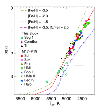
Figure 1: Investigated stars with 12 Gyr isochrones from Yi et al. (2004). The revised stellar parameters for the UMa ii S1 star are linked with the previous ones with a dash. Data from M17a and P19 are shown for comparison. The large cross indicates log g and $T_{\rm eff}$ error bars of 0.2 dex and 150 K, respectively.

3.6 Comparison with the literature

Coma Berenices. Using spectroscopic method based on the LTE analyses of the Fe i excitation and Fe i-Fe ii ionization balance, F10 derived $T_{\rm eff}$ /log g = 4700/1.3, 4600/1.4, and 4600/1.0 for S1, S2, and S3 stars, respectively. Our $T_{\rm eff}$ and log g values are higher by up to 200 K and 0.7 dex, respectively (Fig. 2), and this is understandable. Spectroscopic temperatures determined from the Fe i lines appear to be systematically lower compared with photometric $T_{\rm eff}$, by 70 to 270 K depending on $T_{\rm eff}$, as shown by Frebel et al. (2013), and LTE leads to systematically lower surface gravity determined from lines of Fe i and Fe ii  (see, for example, Mashonkina et al., 2011).

Segue 1. For S1, S2, and S3 stars, the adopted effective temperatures are consistent with those of Frebel et al. (2014) and the difference in $T_{\rm eff}$ between the two studies is within 50 K. Frebel et al. (2014) corrected their spectroscopic $T_{\rm eff}$ with an empirical relation between photometric and spectroscopic temperatures, as determined by Frebel et al. (2013). For Seg 1 S1, S2, and S3, the differences in surface gravities log g (TS) – log g (F14) = 0.36, 0.14, and 0.20, respectively. Lower log g in F14 can be explained by application of LTE analysis of Fe i and Fe ii lines for log g determination. Seg 1 S4, S5, and S6 stars are a different case. Photometric temperatures of SGM11 adopted in this study are 293 K and 214 K lower and 470 K higher, respectively, compared to those of F14. For S4, S5, and S6, the difference log g (TS) – log g (F14) = $-0.68$, $-0.45$, and 0.73, respectively, and it is mainly caused by differences in $T_{\rm eff}$.

For Seg 1 S7, its $T_{\rm eff}$ is well fixed. We adopted $T_{\rm eff}$ = 5000 K, which is consistent with photometric T(V$-$K) = 4997 K and T(V$-$J) = 4983 K values derived with the RM05 calibration and $T_{\rm eff}$ = 4960 K from Norris et al. (2010). We adopted the distance based log g = 2.40, which is 0.5 dex higher compared to that of Norris et al. (2010), derived from isochrones.

Triangulum ii. For Tri ii S40, our $T_{\rm eff}$/log g = 4900/1.87 are in agreement with 4800/1.80 derived by Venn et al. (2017), using similar methods. Parameter determinations based on Fe i and Fe ii line analysis in LTE results in lower $T_{\rm eff}$ and log g of 4720/1.35 and 4816/1.64, found by Ji et al. (2019) and Kirby et al. (2017), respectively.

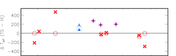
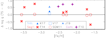
Figure 2: Comparison of the derived $T_{\rm eff}$ and log g with the literature data. See Sect. 3.6 for details.

4 Chemical abundances

4.1 Spectral observations

For ComaBer S1, S2, S3, Tri ii S40, and Seg 1 S3, observed spectra (R = 34 000) are taken from the archive of the Keck telescope (Program ID C168Hr, C222Hr, and C332Hr). Norris et al. (2010) observed Seg 1 S7 with UVES/VLT, and we took its spectrum from the ESO archive (Programme ID 383.B-0093(A)). For the remaining Seg 1 stars, we use spectra taken with MIKE/Magellan spectrograph/telescope and reduced in the original study of Frebel et al. (2014).

4.2 Method of calculation

For our sample stars, element abundances are determined using the synthetic spectrum method by fitting line profiles to high-resolution observed spectra. Theoretical spectra were calculated using the synthV_NLTE code (Tsymbal et al., 2019) integrated to the idl binmag code by O. Kochukhov. This technique allows to obtain the best fit to the observed spectrum with the NLTE effects taken into account via pre-calculated departure coefficients for a given model atmosphere.

The coupled radiative transfer and statistical equilibrium equations were solved with a revised version of the detail code (Butler & Giddings, 1985). The update was presented by Mashonkina et al. (2011).

We used classical plane-parallel model atmospheres interpolated for a given $T_{\rm eff}$, log ${g}$, and [Fe/H] from the marcs model grid (Gustafsson et al., 2008).

The full list of the investigated lines is presented in Table 4 along with gf-values, excitation energies of the lower levels, and the derived NLTE and LTE abundances for the sample stars. The line list for synthetic spectrum calculation was extracted from the Vienna Atomic Line Database (VALD, Ryabchikova et al., 2015). The isotopic splitting is taken into account for the Ca ii resonance and IR triplet lines and Ba ii lines. For the lines of Sc ii, V i, Mn i, Co i, and Ba ii we take into account their hyperfine splitting (HFS) structure, using the HFS data implemented to the VALD database by Pakhomov et al. (2019). To determine barium abundances, we assume the r-process isotopic ratio $\rm{Ba^{\rm 135}:Ba^{\rm 137}:Ba^{\rm 138}}$ = 0.26:0.20:0.54 from Arlandini et al. (1999).

Table 4: NLTE and LTE abundances from individual lines of the sample stars.

species	$\lambda$	Eexc	log gf	EW	$\log\varepsilon_{\rm NLTE}$	$\log\varepsilon_{\rm LTE}$
	Å	eV		mÅ
Seg1 S1:
Na I	5889.95	0.00	0.11	190.8	3.88	4.19
Na I	5895.92	0.00	–0.19	171.7	3.90	4.30
This table is available in its entirety in a machine-readable form in the online journal. A portion is shown here for guidance regarding its form and content.

4.3 NLTE effects

Abundances of O, Na, Mg, Al, Si, Ca, Ti, Fe, Sr, and Ba were determined using the NLTE line formation calculations with comprehensive model atoms developed and tested in our earlier studies. For mechanisms of the departures from LTE and the details of the NLTE calculations for the above chemical elements, see references in Table 5. Here we briefly describe the impact of NLTE on abundance determinations.

In atmospheres of cool metal-poor giants, NLTE may lead to significant changes in abundances and abundance ratios compared to LTE. For Mg i, Al i, Ca i, Ti i, and Fe i, NLTE leads to higher abundances, up to 0.2 dex, depending on species, atmospheric parameters, and adopted spectral lines. For O i, Na i, and K i, NLTE leads to lower abundances, up to 0.5 dex in our sample stars. For Sr ii and Ba ii in the sample stars, NLTE leads to nearly 0.1 dex higher average abundance. For Si i, Fe ii, and Ti ii, NLTE effects are negligible.

Our [Fe/H] is based on Fe ii lines, thus shifts in [El/Fe] abundance ratios due to NLTE are dominated by NLTE effects for a given element. The largest shift is found for [Na/Mg] abundance ratios, since, for Na i and Mg i, NLTE leads to changes of different signs. For more details on the impact of NLTE on abundances of the above chemical elements in the atmospheres of VMP giants see Fig. 1 in Mashonkina et al. (2017b).

Table 5: Model atoms for the NLTE calculations performed in this study.

species	reference	H i collisions
O I	Sitnova & Mashonkina (2018)	BVM19
Na I	Alexeeva et al. (2014)	BBD10
Mg I	Mashonkina (2013)	BBS12
Al I	Baumueller & Gehren (1996)	B13
Si I	Mashonkina (2020)	BYB14
K I	Neretina et al. (2020)	YVB19
Ca I-II	Mashonkina et al. (2007)	BVY17-BVG18
Ti I-II	Sitnova et al. (2016)	SYB20
Fe I-II	Mashonkina et al. (2011)	$S_{\rm H}$ = 0.5
Sr II	Belyakova & Mashonkina (1997)	$S_{\rm H}$ = 0.01
Ba II	Mashonkina et al. (1999)	BY18
BVM19 = Belyaev et al. (2019), BBD10 = Barklem et al. (2010), BBS12 = Barklem et al. (2012), B13 = Belyaev (2013), BYB14 = Belyaev et al. (2014), YBV19 = Yakovleva et al. (2019), BVY17 = Belyaev et al. (2017), BVG18 = Belyaev et al. (2018), SYB20 = Sitnova et al. (2020), BY18 = Belyaev & Yakovleva (2018), $S_{\rm H}$ is a scaling coefficient to the Drawin (1968) formula.

For C, Sc, V, Cr, Mn, Ni, Co, and Zn, we determined LTE abundances and applied the NLTE abundance corrections (differences between NLTE and LTE abundances from individual lines, $\Delta_{\rm NLTE}$ = $\log\varepsilon_{\rm NLTE}-\log\varepsilon_{\rm LTE}$) from the literature, where available.

Carbon abundances were derived from molecular CH bands in the blue spectral region at 4300-4400 Å. NLTE calculations for lines of CH molecules, as well as for other molecules in stellar atmospheres are not available. Alexeeva & Mashonkina (2015) showed that the LTE abundances from CH lines are consistent with the NLTE abundance from C i  lines in a sample of cool metal-poor stars, when using classical model atmospheres. We thus adopted the LTE abundances from CH lines.

We determined scandium abundances from lines of Sc ii. In atmospheres of cool stars, Sc ii is a majority species, and minor NLTE abundance corrections could be expected. NLTE calculations for Sc ii in the atmospheres of cool dwarf stars were presented by Zhang et al. (2008) and Zhao et al. (2016). At metallicity below [Fe/H] $\simeq-1$, the NLTE abundance corrections for Sc ii lines are slightly positive and are less than 0.05 dex. The NLTE effects for Sc ii were thus ignored.

Zinc abundances were determined from only one line, Zn i 4810 Å. To account for deviations from LTE, we applied the NLTE abundance corrections from Takeda et al. (2005). For very metal-poor (VMP) giants, $\Delta_{\rm NLTE}$ for Zn i 4810 Å ranges from $-0.02$ to 0.12 dex depending on $T_{\rm eff}$, log g, and EW. We applied $\Delta_{\rm NLTE}$ = 0.05 dex, which corresponds to lines with EW $\simeq$ 20 mÅ, as observed in our sample stars.

NLTE calculations for neutral species with ionization energy below 8 eV, such as Ti i (Bergemann, 2011), Cr i (Bergemann & Cescutti, 2010), Mn i (Bergemann & Gehren, 2008), Fe i (Mashonkina et al., 2011), and Co i (Bergemann et al., 2010) report an overionization, which leads to weakened lines and positive NLTE abundance corrections.

To determine the NLTE abundance from lines of Cr i, we adopted abundance corrections calculated with the model atom of Bergemann & Cescutti (2010) and available at the MPIA website. For the sample stars, NLTE abundance corrections for Cr i lines vary from 0.20 to 0.45 dex depending on the line and stellar parameters.

Our manganese abundances or upper limits rely on the subordinate Mn i 4783 Å and 4823 Å lines. For all sample stars, we applied the same NLTE abundance corrections of 0.3 dex as calculated by Bergemann et al. (2019) for model atmosphere with $T_{\rm eff}$/log g/[Fe/H] = 4500/1.5/$-2$.

For V i, Co i and Ni i, the literature data on NLTE effects are either missing or poor and cannot be applied for abundance correction. NLTE calculations for V i have never been performed. The statistical equilibrium calculations for Ni i in the solar atmosphere were presented by Bruls (1993) and Vieytes & Fontenla (2013), however, they did not study NLTE effects on atmospheres with different parameters and the impact of NLTE on abundance determination. NLTE calculations for Co i- ii were performed by Bergemann et al. (2010). In cool MP stars, they found large positive NLTE abundance corrections of up to 0.8 dex. For Co i 4121 Å in our sample stars, $\Delta_{\rm NLTE}$ ranges from 0.41 to 0.75 dex according to the data from the MPIA website. Observations of MP stars argue for overestimated NLTE effects in Bergemann et al. (2010). For example, in a halo giant HD 122563 with well-determined stellar parameters, we found LTE abundance difference between lines of neutral and ionized species of $\log\varepsilon$(Co i 4110,4121 Å) – $\log\varepsilon$(Co ii 3501 Å) = $-0.08$ dex (Table 6). The NLTE calculations of Bergemann et al. (2010) predict $\Delta_{\rm NLTE}=0.72$ dex and 0.69 dex for Co i 4110 Å and 4121 Å, respectively, while minor $\Delta_{\rm NLTE}$ for Co ii 3501 Å, and thus do not allow to fulfil an ionization balance. To make these estimates for HD 122563, we adopted $T_{\rm eff}$ = 4600 K, log g = 1.4, [Fe/H] = $-2.55$, and $\xi_{\rm t}$= 1.6 km s^-1 as in Mashonkina et al. (2019).

For V i, Co i and Ni i, we applied an empirical strategy to account for deviations from LTE. For a sample of VMP giants, Mashonkina et al. (2017b) found [Ni i/Fe i] $\sim$ 0, when abundances from Ni i and Fe i are taken in LTE. This argues for similar values for the NLTE abundance corrections for both Ni i and Fe i. To account for NLTE effects for Ni i, V i, and Co i, we provide the final abundance ratios as [El/Fe i]_LTE. We note that for Ni i and Co i, this strategy provides realistic results, while it underestimates NLTE effects for V i. For example, in HD 122563, V i – V ii = $-0.52$ dex in LTE (Table 6), while Fe i – Fe ii = $-0.25$ dex as determined in Mashonkina et al. (2019).

4.4 Stellar abundances

Table 6: LTE abundances of selected chemical species in HD 122563.

Species	Sc ii	V i	V ii	Co i	Co ii	Ni i	Zn i
${\rm[El/Fe]}$	0.05	–0.52	0.00	–0.09	0.02	–0.18	–0.07
$\sigma$	0.03		0.07	0.06		0.10
Nlines	3	1	3	3	1	9	1
gf from	L19	L14	W14	L15	R98	WL14,	W68
						F88
We adopted [Fe/H] = $-2.55$ from NLTE analyses of Mashonkina et al. (2019).
L19 - Lawler et al. (2019), L14 - Lawler et al. (2014), W14 - Wood et al. (2014), L15 - Lawler et al. (2015), R98 - Raassen et al. (1998), WL14 - Wood et al. (2014), F88 - Fuhr et al. (1988), W68 - Warner (1968).

The LTE and NLTE (where available) abundances of up to 18 chemical elements for the sample stars are presented in Table 4. In the Appendix, we show standard [El/Fe] versus [Fe/H] diagrams, where our results for Coma Berenices, Segue 1, and Triangulum ii are plotted together with those from M17b and P19 for the MW halo, classical dSphs Sculptor, Ursa Minor, Fornax, and Sextans, and the UFDs Boötes I, UMa ii, and Leo iv.

Element abundance patterns in the range from O to Zn are displayed in Fig. 3 for individual stars in Seg 1, Tri ii, and ComaBer UFDs. For comparison, we indicate the [El/Fe] elemental ratios, which are typical for the MW halo in the $-4<$ [Fe/H] $<-2$ regime, as derived in the literature. They are based on the NLTE abundances from M17b (Na, Mg, Al, Si, Ca, Ti), Zhao et al. (2016, K, Sc), Bergemann & Cescutti (2010, Cr), and Bergemann & Gehren (2008, Mn). Based on our LTE analysis of V ii lines in HD 122563 (Table 6), we adopted [V/Fe] = 0 for the MW halo. This is in line with a comprehensive LTE study of vanadium abundance in 255 halo stars performed by Ou et al. (2020). For [Ni/Fe], we took [Ni i/Fe i] = 0, as obtained by M17b. Abundances of Co and Zn grow toward lower metallicity in the MW halo (see, for example Cayrel et al., 2004; Takeda et al., 2005; Yong et al., 2013). Therefore, for each of [Co/Fe] and [Zn/Fe], we indicate in Fig. 3 two values of 0 and 0.5, which correspond to [Fe/H] $\sim-2$ and $\sim-4$, respectively.

Abundance ratios of the neutron-capture elements, represented by Sr and Ba, are discussed in more detail in Section 5.3.

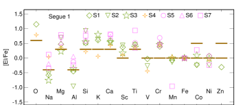
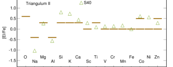
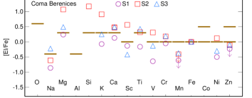
Figure 3: The NLTE element abundance patterns of stars in Seg 1 (top panel), Tri ii (middle panel), and ComaBer (bottom panel) UFDs. Mean abundance ratios for metal-poor MW halo stars are shown with dashes.

4.4.1 Segue 1 UFD

Carbon. Seg 1 S1, S2, and S3 stars have normal nearly solar [C/Fe], ranging from $-0.11$ to 0.08. Seg 1 S4 has [C/Fe] = 0.74 and gained this carbon enhancement from its companion. S5 has carbon enhancement [C/Fe] of 1 dex. The strength of CH lines decreases steeply with increasing $T_{\rm eff}$ and they become weak in S6 with $T_{\rm eff}$ = 5640 K. We estimated [C/Fe] $<1$ dex for this star. A very high [C/Fe] = 2.30 was found in S7. Our results are in agreement with earlier determinations of F14 and N10. We note that in S5, S6, and S7 with luminosity of L/L_⊙ = 1.33, 1.07, and 1.69, respectively, the carbon enhancement is caused by high carbon abundance in the gas at the epoch of their formation, but not carbon dredge-up from the stellar interiors due to stellar evolution.

$\alpha$-elements. In the most metal-rich sample stars S1 and S4, we detected the O i 7771 Å triplet lines and found high [O/Fe] = 1.15 and 0.79, respectively. This is the first measurement of oxygen abundance in Segue 1.

For each of Mg, Si, Ca, and Ti, the stars in Segue 1 reveal enhancements relative to Fe in line with the earlier conclusions of F14. However, in contrast to similar [$\alpha$/Fe] of 0.5 dex found by F14 for different elements and stars, our [$\alpha$/Fe] ranges from 0.2 to 0.9 dex depending on a star and chemical element.

Sodium and Aluminium. We found low [Na/Fe] from $-0.76$ to $-0.53$ in S1, S2, and S3 stars, which have [Fe/H] $>-2.4$, while more metal-poor S5, S6, and S7 have higher [Na/Fe] from $-0.34$ to 0.12 dex. S4 does not follow this trend, since it gained high sodium from its binary companion. This result is qualitatively in line with F14. However, due to application of NLTE, [Na/Fe] in this study are significantly lower, compared to LTE ratios of F14.

A similar behaviour is found for aluminium, with [Al/Fe] from $-0.24$ to 0.05 in stars with [Fe/H]$<-3.1$, and lower [Al/Fe] from $-0.96$ to $-0.37$ in stars with [Fe/H] $>-2.4$.

Potassium. Inspecting the spectra of Seg 1 stars, we detected the resonance line K i 7698 Å in S1, S2, S3, and S4. In S1, S2, and S3, we found high [K/Fe] of 0.61, 0.63, and 0.80, respectively, while S4 has lower [K/Fe] = 0.06. This is the first measurement of potassium in Segue 1.

Scandium and Vanadium. We found nearly solar [V/Fe] in S1, while lower [V/Fe] = $-0.26$ and $-0.44$ in S2 and S4, respectively. Seg 1 stars are enhanced in scandium with [Sc/Fe] from 0.11 in S4 to 0.43 in S2. Scandium abundance does not follow vanadium, and [Sc/V] ratio is about 0.5 dex, on average.

Iron-peak elements. In all Seg 1 stars, we found chromium abundance to be enhanced with respect to iron, with [Cr/Fe] from 0.14 to 0.69 dex. Our [Cr/Fe] ratios are higher compared to those of F14, derived in LTE.

In the majority of Seg 1 stars, manganese follows iron with [Mn/Fe] from $-0.14$ to 0.04 dex. An exception is S7, with low [Mn/Fe] = $-0.96$ dex.

Cobalt abundance follows iron within the error bars, however, [Co/Fe] slightly decreases with [Fe/H] from 0.28 dex in S5 to $-0.24$ in S1 and S2. This result is in line with F14 and [Co/Fe] of metal-poor MW halo stars (Cayrel et al., 2004; Yong et al., 2013).

In the majority of Seg 1 stars, nickel abundance follows iron within 0.1 dex, while lower [Ni/Fe] = $-0.23$ and $-0.24$ are found in S2 and S7, respectively.

An abundance of Zn is determined only in S1 and it yields [Zn/Fe] = $-0.31$.

Neutron capture elements. In five Segue 1 stars, lines of Sr and Ba stars are too weak to be detected even in the S1 star with [Fe/H] = $-1.6$, which argues for missing sources of neutron-capture element production at the early stage of Segue 1 formation. The lines of strontium and barium are detected in Seg 1 S7, and this is the first barium abundance determination in this star. Due to high carbon overabundance, the only Ba ii 4934 line available in the spectrum is blended with the CH lines, as shown in Fig. 4. The nearby lines are fitted well, and we believe that their contribution to the Ba ii 4934 line is evaluated correctly. Another star, where strontium and barium lines can be measured is S4, a carbon rich star, enhanced with neutron-capture elements as found by F14. The abundance pattern of this star follows that of the s-process. Its initial chemical composition was contaminated by its binary companion. We excluded neutron-capture element abundances of S4 from our analysis.

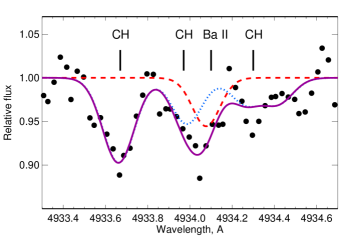
Figure 4: Ba ii 4934 line blended with CH molecular lines in the observed spectrum of Seg 1 S7 (circles). The best fit synthetic spectrum (solid line) is plotted together with spectrum calculated without carbon (dashed line) and without barium (dotted line).

4.4.2 Coma Berenices UFD

Carbon. Coma Berenices S1 and S2 with luminosities log(L/L_⊙) $<$ 2.3 show [C/Fe] = $-0.21$ and $-0.11$, while more luminous S3 with log(L/L_⊙) = 2.4 is depleted in carbon with [C/Fe] = $-0.78$. This corresponds to the carbon-normal stellar populations of dwarf spheroidal galaxies (see, for example, Fig. 7 in Jablonka et al., 2015). These ratios are slightly lower compared to those, found in F10. However, this difference does not impact on classification of ComaBer stars as carbon normal.

$\alpha$-elements. ComaBer stars are enhanced in $\alpha$-elements relative to iron. However, different elements in a given star and a given element in different stars show different [El/Fe] abundance ratios. S3 shows [$\alpha$/Fe] of 0.5 for Mg and Ca and 0.4 for Ti. S2 is extremely enhanced in magnesium and silicon with [Mg/Fe] = 1.07 and [Si/Fe] = 1.17, while calcium and titanium enhancements are lower with [Ca/Fe] = 0.48 and [Ti/Fe] = 0.32. S1 has the highest [Fe/H] = $-2.1$ and shows lower compared to S2 and S3 [$\alpha$/Fe] = 0.24 and 0.13 for Mg and Ca and [Ti/Fe] = $-0.28$. Our results are in line with F10. The possible causes of low [$\alpha$/Fe] in ComaBer S1 are discussed in Section 5.1.

Sodium is underabundant with respect to iron in all ComaBer stars. Different stars show different [Na/Fe] = $-0.86$, $-0.61$, and $-0.22$ in S1, S2, and S3, respectively. We confirm a very low sodium abundance in ComaBer S1 compared to the MW halo stars and stars in other dwarf galaxies, as found by F10. However, our NLTE [Na/Fe] are much lower than those of F10 determined in LTE.

Potassium. Inspecting the spectra of ComaBer S1, S2, and S3, we detected the resonance K i 7698 Å. We found high overabundance [K/Fe] = 0.91 in ComaBer S2. ComaBer S3 shows moderate [K/Fe] = 0.25, while lower [K/Fe] = $-0.07$ was found in ComaBer S1. This is the first measurement of potassium in ComaBer.

Scandium and Vanadium. ComaBer stars show a scatter of 1 dex in [V/Fe] and [Sc/Fe]. S2 is enhanced in Sc and V with [Sc/Fe] = 0.56 and [V/Fe] = 0.34, while S1 and S3 are depleted and show negative [Sc/Fe] and [V/Fe]. For scandium and vanadium, our results are in line with F10.

Iron-peak elements. Chromium abundance follows iron in S1, with [Cr/Fe] = $-0.05$, while S2 and S3 have higher [Cr/Fe] of 0.2 dex. For S1, our [Cr/Fe] is consistent within the error bars with those of F10, while for S2 and S3, F10 found lower [Cr/Fe] = $-0.54$ and $-0.34$ dex, respectively. This discrepancy can be partially explained with the NLTE effects.

Manganese abundances are low in ComaBer stars, with [Mn/Fe] = $-0.37$ in S3. We estimated upper limits [Mn/Fe] $<-0.61$ and $<-0.41$ for S1 and S2, respectively. Our estimations are consistent with those of F10.

ComaBer S1, S2, and S3 stars have different [Ni/Fe] of $-0.50$, 0.12, and $-0.29$, respectively. At least three lines of Ni i were adopted for abundance determination. Similar [Ni/Fe] = $-0.56$, 0.08, $-0.19$ were found by F10 in S1 S2, and S3, respectively.

In ComaBer S2, S3, and S1 zinc is underabundant with respect to iron, and [Zn/Fe] = $-0.11$, $-0.10$, and $<-0.23$ dex, respectively. Our values are close to those of F10.

Neutron capture elements. We found [Sr/Fe] = $-1.97$, $-1.82$ and $-1.63$ in ComaBer S1, S2, and S3, respectively. These values are higher compared to those of F10.

Barium abundances in ComaBer span a wide range, and [Ba/Fe] = $-2.32$, $-1.64$, and $-1.02$ in S1, S2, and S3, respectively. Our [Ba/Fe] in S1 is similar to that of F10, while for S2 and S3, we found 0.3 dex lower [Ba/Fe].

For ComaBer S3, we derived [Sr/Ba] = $-0.61$. This value is close to the empirical estimates of pure r-process ratio: [Sr/Ba]_r = $-0.44$ (Barklem et al., 2005) and $-0.38$ (Mashonkina et al., 2017b). The higher [Sr/Ba] = 0.35 was found in ComaBer S1. See Section 5.3 for a discussion of strontium and barium abundances in stars in different galaxies.

4.4.3 Triangulum ii UFD

LTE abundance analysis of Tri ii S40 star was presented by Kirby et al. (2017), Venn et al. (2017, hereafter V17), and Ji et al. (2019, hereafter J19) using different high-resolution spectra. We adopted spectral observations of K17, since they managed to measure the largest number of chemical species compared with the other two studies. When presenting our results, we focus mainly on the comparison with K17. We note that for the chemical elements in common (Na, Mg, K, Ca, Ti, Cr, Fe, and Ni) the abundance difference between different studies does not exceed 0.4 dex. Consistent within 0.1 dex abundances were found in K17 and J19, an exception is chromium, where the difference between the two studies amounts to 0.25 dex.

$\alpha$-elements. Tri ii S40 has moderate $\alpha$-enhancement with [$\alpha$/Fe] = 0.19, 0.47, and 0.09 for Mg, Ca, and Ti, respectively. Very similar [$\alpha$/Fe] ratios of 0.24, 0.40, and 0.14 were found by K17 for the same elements. K17 determined an upper limit for [Si/Fe]$<0.76$ from weak Si i 6155 Å line. We adopted Si i 4102 Å line with EW = 84.3 mÅ for abundance determination and found a high [Si/Fe] = 0.80.

Sodium and Aluminium. Tri ii S40 has very low [Na/Fe] = $-1.03$, while normal [Al/Fe] = $-0.56$. Low sodium was reported by K17, with [Na/Fe] = $-0.81$ in LTE. K17 found higher [Al/Fe] = 0.

Potassium. We found a high [K/Fe] = 0.73. This value is lower compared to [K/Fe] = 0.88 found by K17 in LTE.

Scandium and Vanadium. Tri ii S40 shows nearly normal [V/Fe] = $0.14$, while enhanced [Sc/Fe] of 0.29. These ratios are consistent within the error bars with those of K17.

Iron-peak elements. We found chromium abundance to be moderately enhanced with respect to iron, with [Cr/Fe] = 0.14, in contrast to low [Cr/Fe] = $-0.45$ found by K17 in LTE.

Tri ii S40 has a high [Co/Fe] = 0.62. This value is higher than [Co/Fe] = 0.13 found by K17 in LTE.

We found high [Ni/Fe] = 0.56, which is close to [Ni/Fe] = 0.53 found in K17.

A moderate enhancement was found for zinc, with [Zn/Fe] = 0.29. Slightly higher ratio [Zn/Fe] = 0.40 was obtained in K17.

Neutron-capture elements We found [Sr/Fe] = $-1.94$, which differs from [Sr/Fe] = $-1.51$ determined by K17. The discrepancy in abundances is caused by observed spectra employed (see the Appendix). For S40, we adopted archival spectra, reduced in a slightly different manner, compared to K17. Each of Sr ii lines is displaced at the edge of the echelle order, and the uncertainty in accounting for the scattered light can be the source of discrepancies in EWs (see the Appendix). For Sr ii 4077Å and 4215Å lines, our best-fit synthetic spectra correspond to EW = 59.6 and 45.1 mÅ, respectively, while K17 provides EW = 79.0 and 89.3 mÅ. Using the EWs from K17, we obtained a discrepancy of 0.4 dex between abundances from the two lines, while our measurements lead to similar abundances from both lines. We obtained [Ba/Fe] = $-2.07$, while lower value [Ba/Fe] = $-2.37$ was found in K17. See Section 5.3 for a discussion of strontium and barium abundances in stars in different galaxies.

Table 7: The derived element abundances in the sample stars.

Sp.	$\log\varepsilon_{\rm\odot}$	Nl	$\log\varepsilon_{\rm LTE}$	$\log\varepsilon_{\rm NLTE}$	[El/H]	[El/Fe]
Segue 1 S1
CH	8.39	1	6.79 (0.10)		–1.60	0.11
O I	8.73	1	8.33 (0.10)	8.17 (0.10)	–0.56	1.15
Na I	6.33	2	4.39 (0.04)	4.04 (0.04)	–2.29	–0.58
Mg I	7.58	2	6.34 (0.01)	6.33 (0.15)	–1.25	0.47
Al I	6.47	1	4.12 (0.10)	4.31 (0.10)	–2.16	–0.45
Si I	7.52	3	6.36 (0.12)	6.32 (0.11)	–1.20	0.51
K I	5.12	1	4.62 (0.10)	4.02 (0.10)	–1.10	0.61
Ca I	6.36	16	5.26 (0.14)	5.24 (0.15)	–1.12	0.60
Sc II	3.10	4	1.76 (0.24)	1.76 (0.24)	–1.34	0.37
Ti I	4.90	7	3.33 (0.23)	3.36 (0.24)	–1.54	0.17
Ti II	4.90	23	3.68 (0.24)	3.66 (0.25)	–1.24	0.47
V I	4.00	2	2.28 (0.05)		–1.72	–0.03
Cr I	5.65	7	3.70 (0.15)	4.33 (0.16)	–1.32	0.39
Mn I	5.37	3	3.29 (0.04)	3.59 (0.04)	–1.78	–0.07
Fe I	7.50	58	5.81 (0.25)	5.83 (0.25)	–1.67	0.04
Fe II	7.50	17	5.79 (0.18)	5.79 (0.18)	–1.71	0.00
Co I	4.92	2	3.00 (0.15)		–1.92	–0.23
Ni I	6.23	12	4.61 (0.28)		–1.62	0.07
Zn I	4.62	1	2.55 (0.10)	2.60 (0.10)	–2.02	–0.31
Segue 1 S2
CH	8.39	1	6.09 (0.10)		–2.30	0.08
Na I	6.33	2	3.94 (0.26)	3.42 (0.25)	–2.91	–0.53
Mg I	7.58	3	5.82 (0.06)	5.89 (0.16)	–1.69	0.70
Al I	6.47	1	2.78 (0.10)	3.13 (0.10)	–3.34	–0.96
Si I	7.52	2	6.08 (0.12)	6.07 (0.11)	–1.45	0.93
K I	5.12	1	3.73 (0.10)	3.37 (0.10)	–1.75	0.63
Ca I	6.36	12	4.43 (0.12)	4.49 (0.13)	–1.87	0.51
Sc II	3.10	3	1.15 (0.08)	1.15 (0.08)	–1.95	0.43
Ti I	4.90	5	2.85 (0.11)	2.99 (0.13)	–1.91	0.48
Ti II	4.90	20	3.00 (0.14)	2.97 (0.16)	–1.93	0.45
V I	4.00	1	1.42 (0.10)		–2.58	–0.26
Cr I	5.65	7	3.05 (0.20)	3.73 (0.17)	–1.92	0.46
Mn I	5.37	2	2.55 (0.10)	2.85 (0.10)	–2.52	–0.14
Fe I	7.50	74	5.18 (0.24)	5.25 (0.24)	–2.25	0.13
Fe II	7.50	11	5.12 (0.13)	5.12 (0.13)	–2.38	0.00
Co I	4.92	3	2.36 (0.19)		–2.56	–0.24
Ni I	6.23	2	3.68 (0.22)		–2.55	–0.23
Segue 1 S3
CH	8.39	1	5.99 (0.10)		–2.40	–0.11
Na I	6.33	2	3.66 (0.06)	3.28 (0.02)	–3.05	–0.76
Mg I	7.58	2	5.47 (0.02)	5.52 (0.02)	–2.06	0.23
Al I	6.47	1	3.49 (0.10)	3.81 (0.10)	–2.66	–0.37
Si I	7.52	1	5.78 (0.10)	5.78 (0.10)	–1.74	0.55
K I	5.12	1	3.90 (0.10)	3.63 (0.10)	–1.49	0.80
Ca I	6.36	12	4.53 (0.13)	4.61 (0.14)	–1.75	0.54
Sc II	3.10	3	0.98 (0.02)	0.98 (0.02)	–2.12	0.17
Ti I	4.90	6	3.01 (0.10)	3.18 (0.12)	–1.72	0.57
Ti II	4.90	18	3.01 (0.23)	2.98 (0.26)	–1.92	0.37
Cr I	5.65	6	3.11 (0.15)	3.82 (0.15)	–1.83	0.46
Mn I	5.37	2	2.77 (0.12)	3.07 (0.12)	–2.30	0.00
Fe I	7.50	63	5.12 (0.18)	5.20 (0.18)	–2.30	–0.01
Fe II	7.50	12	5.21 (0.10)	5.21 (0.10)	–2.29	0.00
Co I	4.92	1	2.64 (0.10)		–2.28	0.10
Ni I	6.23	1	3.84 (0.10)		–2.39	–0.01
Ba II	2.13	1	–1.50 (0.10)	–1.30 (0.10)	–3.43	–1.14
Segue 1 S4, CEMP-s star
CH	8.39	1	7.44 (0.10)		–0.95	0.74
O I	8.73	2	7.98 (0.09)	7.83 (0.07)	–0.90	0.79
Na I	6.33	2	5.01 (0.16)	4.68 (0.10)	–1.65	0.04
Mg I	7.58	4	6.26 (0.08)	6.25 (0.01)	–1.33	0.36
Si I	7.52	1	6.10 (0.10)	6.05 (0.10)	–1.47	0.22
K I	5.12	1	4.00 (0.10)	3.49 (0.10)	–1.63	0.06
Ca I	6.36	15	5.10 (0.16)	5.10 (0.22)	–1.26	0.43
Sc II	3.10	2	1.52 (0.37)	1.52 (0.37)	–1.58	0.11

Table 8: continued

Sp.	$\log\varepsilon_{\rm\odot}$	Nl	$\log\varepsilon_{\rm LTE}$	$\log\varepsilon_{\rm NLTE}$	[El/H]	[El/Fe]
Ti I	4.90	5	3.39 (0.18)	3.55 (0.30)	–1.35	0.34
Ti II	4.90	19	3.61 (0.16)	3.58 (0.17)	–1.32	0.37
V I	4.00	1	1.84 (0.10)		–2.16	–0.44
Cr I	5.65	5	3.77 (0.09)	4.40 (0.14)	–1.25	0.44
Mn I	5.37	3	3.42 (0.12)	3.72 (0.12)	–1.65	0.04
Fe I	7.50	55	5.78 (0.19)	5.80 (0.19)	–1.70	–0.01
Fe II	7.50	14	5.81 (0.16)	5.81 (0.16)	–1.69	0.00
Ni I	6.23	6	4.44 (0.16)		–1.79	–0.07
Segue 1 S5, CEMP-no star
CH	8.39	1	5.74 (0.10)		–2.65	0.91
Na I	6.33	2	2.55 (0.11)	2.43 (0.14)	–3.90	–0.34
Mg I	7.58	5	4.68 (0.27)	4.73 (0.24)	–2.85	0.71
Al I	6.47	2	2.21 (0.16)	2.78 (0.18)	–3.69	–0.13
Si I	7.52	1	4.61 (0.10)	4.54 (0.10)	–2.98	0.58
Ca I	6.36	2	3.47 (0.06)	3.60 (0.04)	–2.76	0.80
Ti II	4.90	9	1.76 (0.18)	1.86 (0.17)	–3.04	0.52
Cr I	5.65	2	2.11 (0.01)	2.78 (0.01)	–2.87	0.69
Fe I	7.50	15	3.78 (0.34)	3.94 (0.35)	–3.56	0.00
Ni I	6.23	2	2.58 (0.36)		–3.65	0.07
Segue 1 S6, CEMP-no star
CH	8.39	1	6.19 (0.10)		$<$–2.20	$<$ 1.00
Na I	6.33	2	3.04 (0.03)	2.94 (0.00)	–3.39	–0.20
Mg I	7.58	2	4.80 (0.17)	4.92 (0.12)	–2.66	0.53
Al I	6.47	1	2.69 (0.10)	3.33 (0.10)	–3.14	0.05
Si I	7.52	1	5.34 (0.10)	5.29 (0.10)	–2.23	0.96
Ca I	6.36	3	3.79 (0.26)	3.90 (0.23)	–2.46	0.73
Ti II	4.90	10	1.95 (0.11)	2.06 (0.10)	–2.84	0.35
Cr I	5.65	4	2.26 (0.28)	2.98 (0.23)	–2.67	0.52
Fe I	7.50	12	4.12 (0.23)	4.31 (0.24)	–3.19	–0.00
Segue 1 S7, CEMP-no star
CH	8.39	2	7.21 (0.05)		–1.18	2.30
Na I	6.33	2	3.13 (0.10)	2.97 (0.15)	–3.36	0.12
Mg I	7.58	3	4.85 (0.10)	4.89 (0.16)	–2.69	0.79
Al I	6.47	1	2.43 (0.10)	2.75 (0.10)	–3.72	–0.24
Si I	7.52	1	4.81 (0.10)	4.80 (0.10)	–2.72	0.76
Ca I	6.36	6	3.59 (0.04)	3.70 (0.05)	–2.66	0.81
Ti II	4.90	7	2.28 (0.22)	2.36 (0.22)	–2.54	0.94
Cr I	5.65	3	1.89 (0.11)	2.61 (0.18)	–3.04	0.44
Mn I	5.37	1	0.83 (0.10)	0.93 (0.10)	–4.44	–0.96
Fe I	7.50	21	3.84 (0.14)	3.99 (0.13)	–3.51	–0.03
Fe II	7.50	3	4.02 (0.04)	4.02 (0.04)	–3.48	0.00
Co I	4.92	3	1.54 (0.21)		–3.38	0.28
Ni I	6.23	4	2.33 (0.18)		–3.90	–0.24
Sr II	2.90	2	–2.12 (0.09)	–1.87 (0.05)	–4.77	–1.29
Ba II	2.13	1	–2.42 (0.10)	–2.24 (0.10)	–4.37	–0.89
Tri II S40
Na I	6.33	2	2.66 (0.07)	2.53 (0.15)	–3.80	–1.03
Mg I	7.58	2	4.98 (0.06)	5.08 (0.01)	–2.50	0.27
Al I	6.47	2	2.88 (0.00)	3.14 (0.04)	–3.33	–0.56
Si I	7.52	1	5.55 (0.10)	5.55 (0.10)	–1.97	0.80
K I	5.12	1	3.27 (0.10)	3.08 (0.10)	–2.04	0.73
Ca I	6.36	11	3.88 (0.13)	4.03 (0.12)	–2.33	0.44
Sc II	3.10	4	0.61 (0.12)	0.61 (0.12)	–2.49	0.29
Ti I	4.90	3	2.16 (0.02)	2.44 (0.04)	–2.46	0.32
Ti II	4.90	8	2.21 (0.10)	2.21 (0.11)	–2.69	0.09
V I	4.00	2	1.24 (0.01)		–2.76	0.14
Cr I	5.65	7	2.49 (0.32)	3.01 (0.28)	–2.64	0.14
Mn I	5.37	2	2.47 (0.01)	2.77 (0.01)	-2.60	0.17
Fe I	7.50	40	4.60 (0.13)	4.73 (0.14)	–2.77	0.01
Fe II	7.50	8	4.73 (0.11)	4.73 (0.11)	–2.77	0.00
Co I	4.92	1	2.64 (0.10)		–2.28	0.62
Ni I	6.23	7	3.89 (0.09)		–2.34	0.56
Zn I	4.62	1	2.09 (0.10)	2.14 (0.10)	–2.48	0.29
Sr II	2.90	2	–1.87 (0.01)	–1.82 (0.03)	–4.72	–1.94
Ba II	2.13	1	–2.94 (0.10)	–2.71 (0.10)	–4.84	–2.07

Table 9: continued

Sp.	$\log\varepsilon_{\rm\odot}$	Nl	$\log\varepsilon_{\rm LTE}$	$\log\varepsilon_{\rm NLTE}$	[El/H]	[El/Fe]
Coma Berenices S1
CH	8.39	4	6.18 (0.07)		–2.21	–0.09
Na I	6.33	2	3.54 (0.12)	3.35 (0.18)	–2.98	–0.86
Mg I	7.58	2	5.63 (0.08)	5.69 (0.07)	–1.89	0.24
K I	5.12	1	3.10 (0.10)	2.93 (0.10)	–2.19	–0.07
Ca I	6.36	16	4.29 (0.16)	4.37 (0.20)	–1.99	0.13
Sc II	3.10	4	0.85 (0.15)	0.85 (0.15)	–2.25	–0.13
Ti I	4.90	5	2.51 (0.10)	2.63 (0.09)	–2.27	–0.15
Ti II	4.90	12	2.66 (0.21)	2.62 (0.25)	–2.28	–0.16
V I	4.00	1	1.15 (0.10)		–2.85	–0.64
Cr I	5.65	3	3.10 (0.19)	3.47 (0.25)	–2.18	–0.05
Mn I	5.37	1	$<$ 2.34 (0.10)	$<$ 2.64 (0.10)	$<$ –2.73	$<$ –0.61
Fe I	7.50	33	5.29 (0.18)	5.35 (0.19)	–2.15	–0.03
Fe II	7.50	11	5.38 (0.14)	5.38 (0.14)	–2.12	0.00
Ni I	6.23	3	3.52 (0.06)		–2.71	–0.50
Zn I	4.62	1	$<$ 2.22 (0.10)	$<$ 2.27 (0.10)	$<$ –2.35	$<$ –0.23
Sr II	2.90	1	–1.44 (0.10)	–1.19 (0.10)	–4.09	–1.97
Ba II	2.13	1	–2.41 (0.10)	–2.31 (0.10)	–4.44	–2.32
Coma Berenices S2
CH	8.39	4	5.89 (0.00)		–2.50	0.02
Na I	6.33	2	3.59 (0.01)	3.20 (0.05)	–3.13	–0.61
Mg I	7.58	3	6.05 (0.02)	6.13 (0.16)	–1.45	1.07
Si I	7.52	1	6.22 (0.10)	6.17 (0.10)	–1.35	1.17
K I	5.12	1	3.92 (0.10)	3.51 (0.10)	–1.61	0.91
Ca I	6.36	13	4.26 (0.18)	4.31 (0.19)	–2.05	0.48
Sc II	3.10	3	1.14 (0.05)	1.14 (0.05)	–1.96	0.56
Ti I	4.90	7	2.67 (0.22)	2.87 (0.21)	–2.03	0.49
Ti II	4.90	13	2.69 (0.19)	2.70 (0.21)	–2.20	0.32
V I	4.00	1	1.38 (0.10)		–2.36	0.31
Cr I	5.65	3	2.93 (0.27)	3.31 (0.33)	–2.34	0.18
Mn I	5.37	1	$<$ 2.14 (0.10)	$<$ 2.44 (0.10)	$<$ –2.93	$<$ –0.41
Fe I	7.50	28	4.83 (0.12)	4.91 (0.12)	–2.59	–0.07
Fe II	7.50	5	4.98 (0.15)	4.98 (0.15)	–2.52	0.00
Ni I	6.23	5	3.68 (0.16)		–2.55	0.12
Zn I	4.62	1	1.94 (0.10)	1.99 (0.10)	–2.63	–0.11
Sr II	2.90	1	–1.55 (0.10)	–1.44 (0.10)	–4.34	–1.82
Ba II	2.13	1	–2.15 (0.10)	–2.03 (0.10)	–4.16	–1.64
Coma Berenices S3
CH	8.39	2	5.35 (0.14)		–3.04	–0.65
Na I	6.33	2	4.17 (0.10)	3.72 (0.14)	–2.61	–0.22
Mg I	7.58	3	5.59 (0.03)	5.69 (0.15)	–1.89	0.49
K I	5.12	1	3.16 (0.10)	2.98 (0.10)	–2.14	0.25
Ca I	6.36	18	4.44 (0.09)	4.47 (0.09)	–1.89	0.49
Sc II	3.10	4	0.29 (0.04)	0.29 (0.04)	–2.81	–0.42
Ti I	4.90	8	2.64 (0.10)	2.84 (0.12)	–2.06	0.32
Ti II	4.90	17	2.94 (0.15)	2.94 (0.15)	–1.96	0.43
V I	4.00	1	1.22 (0.10)		–2.55	–0.13
Cr I	5.65	3	3.01 (0.12)	3.45 (0.13)	–2.20	0.19
Mn I	5.37	1	2.31 (0.10)	2.61 (0.10)	–2.76	–0.37
Fe I	7.50	41	5.08 (0.12)	5.16 (0.12)	–2.34	0.05
Fe II	7.50	17	5.12 (0.14)	5.11 (0.13)	–2.39	0.00
Ni I	6.23	8	3.52 (0.04)		–2.71	–0.29
Zn I	4.62	1	2.08 (0.10)	2.13 (0.10)	–2.49	–0.10
Sr II	2.90	1	–1.20 (0.10)	–1.12 (0.10)	–4.02	–1.63
Ba II	2.13	4	–1.32 (0.06)	–1.28 (0.06)	–3.41	–1.02
Ursa Major II S1
Na I	6.33	2	3.26 (0.06)	3.08 (0.01)	–3.25	–0.33
Mg I	7.58	5	4.94 (0.15)	5.07 (0.27)	–2.51	0.41
Ca I	6.36	6	3.56 (0.19)	3.70 (0.19)	–2.66	0.25
Ti I	4.90	3	2.20 (0.20)	2.49 (0.21)	–2.41	0.51
Ti II	4.90	9	2.19 (0.22)	2.20 (0.22)	–2.70	0.22
Fe I	7.50	36	4.50 (0.15)	4.66 (0.15)	–2.84	0.08
Fe II	7.50	7	4.58 (0.13)	4.58 (0.13)	–2.92	0.00
Ni I	6.23	2	3.67 (0.32)		–2.56	0.44
Sr II	2.90	1	–0.95 (0.10)	–0.82 (0.10)	–3.72	–0.80
Ba II	2.13	1	–1.69 (0.10)	–1.45 (0.10)	–3.58	–0.66
Solar abundances from Lodders et al. (2009). The standard
deviations are indicated in parentheses. For V i, Co i, and Ni i,
[El/Fe] are calculated relative to Fe i in LTE.

5 Discussion

5.1 Incomplete mixing in Seg 1 and ComaBer UFDs

Segue 1.

Seg 1 stars show a wide metallicity range, from [Fe/H] = $-1.6$ to $-3.6$. They could be subdivided into two groups according to their chemical properties. The first group contains S1, S2, and S3 with [Fe/H] $>-2.4$, normal carbon abundances and [$\alpha$/Fe]. Star S4, classified as CEMP-s, gained its high carbon and n-capture element abundances from its binary companion, while its $\alpha$-elements and iron-peak elements are suitable for analysis of the chemical history in Segue 1. This star can also be added to the first group with its [Fe/H] = $-1.73$.

Another group contains carbon enhanced S5, S6, and S7 stars with [Fe/H] $<-3.1$. For Na, Al, $\alpha$-elements, these stars have higher [El/Fe] abundance ratios compared to the first group stars (see Fig. 3). Higher [Na/Fe] in more metal-poor stars is not surprising. M17b (see their Fig. 4) found nearly constant [Na/Fe] = $-0.4$ for stars with $-3<$ [Fe/H] $<-2$, while more metal poor stars show an increasing trend with decreasing [Fe/H], up to solar [Na/Fe]. However, for $\alpha$-elements, constant [$\alpha$/Fe] is expected.

In line with F14 and V13, we found all Seg 1 stars to be $\alpha$-enhanced. This argues for an absence of iron, produced in SN ia and a short timescale of star formation. We note that Seg 1 S1 and S4 have fairly high [Fe/H] of $-1.6$ and high [$\alpha$/Fe]. High star formation rate is required to achieve [Fe/H] $\simeq-1.6$ at timescale of less than 1 Gyr, before the onset of iron production in SN ia.

Different stars in Seg 1 show different abundance ratios, which argues for an incomplete mixing of the interstellar medium during the formation of these stars.

Chiaki & Tominaga (2020) investigated how the structure of Pop iii supernova ejecta affects the elemental abundance of extremely metal-poor stars and concluded that single ejecta can produce different abundance patterns of MP stars. According to stellar evolution models, the SN ejecta should be initially stratified, where heavier elements, such as Fe, are in the inner layers and lighter elements, such as C, are in the outer layers. Such a scenario is one of the hypotheses that could explain the observed splitting of Seg 1 stars into two groups (carbon enhanced, with [Fe/H] $<-3.1$ and carbon normal with [Fe/H] $>-2.4$). Accurate chemical enrichment modelling of Seg 1 is required to check this hypothesis.

From analyses of colour-magnitude diagram, coordinates, and proper motions, McConnachie & Venn (2020) found a low membership probability of p = 0.00142 and 0.00024 for Seg 1 S2 and S7, respectively. A membership of Seg 1 S3 and S6 with p = 0.30 and 0.37 is also in doubt. These probabilities were calculated for the Seg 1 structural parameters, d = 22.9 kpc, r_1/2 = 3.95 arcmins, and the eccentricity e = 0.34 (McConnachie & Venn, 2020). However, the structure of faint dwarf galaxies, especially at large radius, can be very complex, and it is known that some of these systems have extended tidal features that are not well captured by the simple parametrisation (Li et al., 2018). For example, Chiti et al. (2020) found members of Tucana ii UFD in its outer region, up to 9 half-light radii. Thus S3 and S6 at distances of 9.54 and 4.5 r_1/2 could be actually members of Seg 1. Anyway, neglecting the above stars would not change our results on the inhomogeneous gas mixing and splitting between carbon-rich and iron-rich stars.

Coma Berenices.

ComaBer stars show close [Fe/H] from $-2.6$ to $-2.1$, however, their [El/Fe] abundance patterns are different. S3 shows normal chemical composition similar to that of the VMP MW halo stars. An exception is low [Sc/Fe] = $-0.42$.

S2 is enhanced in Mg and depleted in sodium, which results in extremely low [Na/Mg] = $-1.68$, which is the lowest value known to date. Due to the high magnesium abundance, this star has high hydrostatic to explosive $\alpha$-element abundance ratios, namely high [Mg/Ca] = 0.59. Stars with high [Mg/Ca] are detected in Hercules dSph (Koch et al., 2008), Draco dSph (Fulbright et al., 2004), Grus ii UFD (Hansen et al., 2020), and the MW (Frebel et al., 2008; Norris et al., 2013; Keller et al., 2014; Depagne et al., 2002; Cohen et al., 2008). A high ratio of hydrostatic to explosive $\alpha$-elements, as observed in these stars, can be produced in SN ii with high progenitor mass (Heger & Woosley, 2010). In addition, there is a hint of inverted odd-even Z effect, namely, odd-Z elements Sc and V are enhanced with respect to their neighbouring even-Z elements Ti and Cr (see Fig. 3). We note the large errors in abundance ratios: [Sc/Ti] = 0.24$\pm 0.22$ and [V/Cr] = 0.37$\pm 0.34$, which prevents us from making a solid conclusion.

S1 shows very low [Na/Fe], it has depleted titanium, vanadium, manganese, nickel, and zinc with respect to iron, and is only moderately enhanced in $\alpha$-elements. S1 is thus enhanced in iron, but not in the other chemical elements. S1 also shows low [Na/Mg] encountered in the literature as a signature of explosions of Population iii stars (see Sect. 5.2 for the discussion and references).

From analysis of medium resolution spectra, Vargas et al. (2013) suggested that the iron excess in S1 and the lower [$\alpha$/Fe] abundance ratios compared to those of S2 and S3 are caused by an onset of iron production in SN ia. To explain low [$\alpha$/Fe] in S1, there is no need to assume an onset of ubiquitous iron production in SNe ia throughout ComBer and extended star formation. It can be explained by formation of S1 in a pocket locally enhanced by a single SN ia event (Ivans et al., 2003; Koch et al., 2008; Venn et al., 2012). Indeed, there are some prompt SN ia with a delay time of less than 500 Myr (Mannucci et al., 2006; Ruiter et al., 2010). Nucleosynthesis calculations of Kobayashi et al. (2020) for SN ia explosions of sub-Chandrasekhar white dwarfs predict [Mn,Ni,Zn/Fe] $<0$, which is similar to what is found in S1.

Another possible explanation for the lower [$\alpha$/Fe] in S1 is its formation from a pocket, where the ejecta of the most massive Type II SNe are missing. This scenario was proposed by Jablonka et al. (2015) to explain the formation of a star in Sculptor dSph, ET0381 with [Fe/H] = $-2.5$, which is poor in all elements with respect to iron. Our abundance analysis cannot solidly recognize the cause of low [$\alpha$/Fe] in S1.

Different chemical element abundance patterns of ComaBer stars argue for an incomplete gas mixing during the formation of this galaxy.

5.2 Footprints of Population iii stars in UFDs.

Despite different [Mg/Fe] and [Na/Fe] found in ComaBer S1, Seg 1 S1, S2, S3, and S5, and Tri ii S40, these stars have very similar low [Na/Mg] from $-1.3$ to $-1.0$. ComaBer S2 shows extremely low [Na/Mg] = $-1.68$, which is the lowest value found in the literature to date.

Low sodium to magnesium abundance ratio of [Na/Mg] $\simeq$ $-1.1$ dex was encountered in the literature and attributed to the odd-even effect, predicted for explosions of Population iii stars (Nomoto et al., 2006; Kobayashi et al., 2006; Tominaga et al., 2007; Heger & Woosley, 2010; Limongi & Chieffi, 2012; Nomoto et al., 2013; Takahashi et al., 2018; Curtis et al., 2019). According to the data from the Stellar Abundances for Galactic Archaeology Database (SAGA Suda et al., 2008, 2017), there are eleven VMP stars with [Na/Mg] $<-1$. Eight of them are in dwarf galaxies, while three are in the MW halo. In addition to the SAGA data, the recent study of Frebel et al. (2019) reported on strong odd-even effect in J0023+0307, with [Na/Mg] = $-1.1$. While the statistics is poor, we note that stars with odd-even effect are more frequent in dwarf galaxies compared to the MW halo.

We selected our sample stars with [Na/Mg] $\leq-1$, namely, ComaBer S1 and S2, Seg 1 S1, S2 and S3, and Tri ii S40 to compare their abundances with predictions of nucleosynthesis in individual explosions of metal-free stars (Fig. 5). It is worth noting that the selected stars do not have any similar abundance ratios except the low [Na/Mg]. M17b found low [Na/Mg] = $-1.3$ in Scl1019417 from the Sculptor dSph and UMa ii S3. In addition to the selected stars, we show in Figure 5 the abundance patterns of Scl1019417 and UMa ii S3.

We tried to fit the derived abundance patterns for elements from C to Zn with the predictions of nucleosynthesis of core-collapse supernovae (CCSNe), hypernovae (HNe), and pair-instability supernova (PISN) of Population iii stars from Tominaga et al. (2007, hereafter TUN07), Heger & Woosley (2010, hereafter HW10), and Takahashi et al. (2018, hereafter TYU18), respectively. Yields from various models of Tominaga et al. (2007) provide [Na/Mg] of $-2.19$ to $-0.19$. We selected the 25-5 and 40B models of TUN07, with [Na/Mg] of $-1.07$ and $-1.86$, respectively, which are close to those in our sample stars. Here, the first number in the designation of models indicates an initial mass of a progenitor star (M_init) and the second symbol indicates a kinetic energy of an explosion at infinity, measured in Bethe (1 B = 10⁵¹ erg), while B means a hypernova with E_k = 30 Bethe. The model of Heger & Woosley (2010) was selected using the starfit.org on-line tool for fitting the stellar element abundance patterns with nucleosynthesis yields. It has M_init = 75M_⊙, E_k = 1.5B, log(f_mix) = $-0.6$, where f_mix is an ejection factor, and predicts [Na/Mg] = $-1.1$. The selected model of TYU18 has M_init = 240M_⊙ and accounts for magnetic field and rotation (MR PISN). The yields of the selected models are plotted in Figure 5.

The only reasonable agreement was found between the predictions of the 25-5 model of TUN07 and the abundance pattern of ComaBer S1, where model predictions and determined abundance ratios are consistent for the ten chemical elements. For potassium, model predictions are 0.4 dex lower compared to the observations. This element is known to be under-produced by models (see, for example, Kobayashi et al., 2006; Kobayashi et al., 2020). The [El/Mg] ratios of Scl1019417 and UMa ii S3 are consistent with the 25-5 model. An exception is the 0.3 dex higher [Ti/Mg] in Scl1019417 and about 0.2 dex lower [Fe/Mg] compared to the model predictions. We note that abundances of potassium in Scl1019417 and UMa ii S3 are not available in M17b.

The 40B model of TUN07 predicts [Na/Mg] = $-1.86$. It was selected to fit the abundance pattern of ComaBer S2 with [Na/Mg] = $-1.68$. However, for the other elements, the model predicts 0.5 dex higher [El/Mg] compared to those observed is S2. There is nothing in common between the model and the abundance pattern of ComaBer S2 except the extremely low [Na/Mg]. This is because the model is Na-poor, while the star is Mg-enhanced.

Individual models predict various chemical element abundance ratios depending on M_init, explosion energy, and other properties of explosions. For example, there are TUN07 models predicting [Mg/Fe] = 0.20 or 1.81 dex, while the majority of these models predict [Mg/Fe] from 0.3 to 0.5 dex. At the early epoch of massive galaxies formation, many SN ii in each mass range enrich the interstellar medium, resulting in a settling of an average [Mg/Fe] of 0.3. This ratio is observed in the majority of MP stars in the MW and classical dSph galaxies. In faint galaxies, only a subset of the full SNe mass range contributes, and the final [Mg/Fe] can differ from a standard average value, depending on stochastically sampled explosions that have enriched a given galaxy. In addition, inhomogeneous mixing of gas results in different element abundance ratios in the next generation of stars. The same is true for other element abundance ratios, such as [Mg/Ca] or [Na/Mg].

Since there are model predictions of explosions of Pop iii stars, producing low [Na/Mg], we suggest them to be responsible for the low [Na/Mg] detected in MP stars. We failed to fit abundance patterns of any of our sample stars with a single nucleosynthesis event, however, we suggest that a small number of SN ii explosions including those with low [Na/Mg] contributed to the abundances found in the investigated stars.

A comparison of observed relative [El/Mg] abundance ratios with nucleosynthesis predictions should be performed with a caution. We note that our sample stars are too metal rich to be fitted with yields from only one explosion. For each selected model, its metallicity is about [Fe/H]$\simeq-3$, which is lower compared to that of the sample stars ($-2.5<$ [Fe/H] $<-2.1$). Magg et al. (2020) estimated analytically a limit for the dilution of metals produced by a single SN and recommended to account for not only element-to-element abundance ratios, but also the absolute abundance values when fitting stellar abundance patterns with nucleosynthesis yields. In their calculations, the following assumptions were adopted: the SN being alone and isolated, the explosions being spherical and well-mixed, and the surrounding medium being homogeneous. The latter assumption is not always fulfilled (see, for example Chiaki & Tominaga, 2020). We also note that to date there is no a metal-poor star, whose extensive abundance pattern is reasonably well fitted with the yields from a single nucleosynthesis episode, despite many attempts that were made (see, for example, Tominaga et al., 2007; Placco et al., 2015; Hansen et al., 2020).

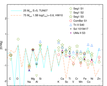
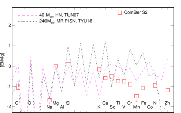
Figure 5: Top panel: Element abundance patterns [El/Mg] of the sample stars with [Na/Mg] $\simeq-1.1$ and model predictions for explosions of metal-free massive stars with M_init = 25M_⊙ (Tominaga et al., 2007, solid curve) and M_init = 75M_⊙ (Heger & Woosley, 2010, dash-dotted curve). For comparison, we show the NLTE [El/Mg] ratios of Scl1019417 and UMa ii S3 from M17b. See the legend for identification of the stars. Bottom panel: Similar plot for ComaBer S2 star with [Na/Mg] = $-1.68$. Dashed and dotted curves show [El/Mg] model predictions for CCSN with M_init = 40M_⊙ (Tominaga et al., 2007) and PISN with M_init = 240M_⊙ (Takahashi et al., 2018).

5.3 Neutron-capture elements in classical and ultra-faint dwarf galaxies

In the majority of EMP stars, n-capture elements are represented by Sr and Ba. A number of the Galactic studies reported on a large scatter of [Sr/Ba], of about 2 dex, which decreases with increasing [Ba/H] (Honda et al., 2004; François et al., 2007; Andrievsky et al., 2011). In classical dSphs, abundances of Sr and Ba at the lowest metallicity are at or below the lowest values in the MW halo, however, the [Sr/Fe] and [Ba/Fe] ratios increase toward the solar ratio as [Fe/H] increases, similarly to that for the MW halo (Cohen & Huang, 2009, 2010; Jablonka et al., 2015; Mashonkina et al., 2017b). Very low abundances of Sr and Ba were reported for the majority of UFDs (Frebel et al., 2010; Simon et al., 2010; Gilmore et al., 2013; Koch et al., 2013; Koch & Rich, 2014; Ji et al., 2016a, c; Nagasawa et al., 2018). In the UFDs, the [Sr/Fe] and [Ba/Fe] ratios do not rise with metallicity, they scatter around a mean floor level of $-1$ and $-0.7$, respectively (M17b). At the same time, the r-process-rich galaxies were discovered, such as Reticulum ii (Ji et al., 2016b; Roederer et al., 2016), Tucana iii (Hansen et al., 2017) and Grus ii (Hansen et al., 2020), providing evidence for a variety of evolution among UFDs. The origin of light neutron-capture elements in VMP stars is not well-understood yet.

In our earlier paper (M17b), it was found that VMP stars in the four classical dSphs (Sculptor, Ursa Minor, Sextans, and Fornax) and in the MW halo form very similar trends on the [Sr/Ba] versus [Ba/H] plane, namely, the data split into two branches: a horizontal one, with a nearly constant [Sr/Ba] $\sim-0.5$, and a well-defined downward trend of [Sr/Ba] with [Ba/H]. Such a behavior of [Sr/Ba] can be explained by two nucleosynthesis processes that occurred in the early Galaxy. The first process is a rapid (r-) process of neutron-capture nuclear reactions. Although astrophysical sites of the r-process are still debated (for a review, see Thielemann et al., 2017), a pure r-process [Sr/Ba]_r ratio was estimated empirically as $-0.44$ (Barklem et al., 2005) and $-0.38$ (M17b).

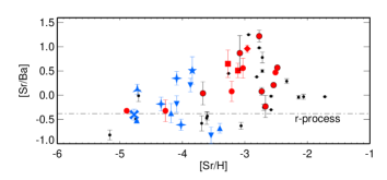
Figure 9: The NLTE [Sr/Ba] abundance ratios for stars in different galaxies. Note a steep [Sr/Ba] increase at [Sr/H] $\simeq-3$ in the MW (black symbols) and classical dSph galaxies (red symbols) and lower [Sr/H] in UFDs (blue symbols) compared to those in massive galaxies. The designations are the same as in Fig. 6.

Observations suggest that the second process operated in a different way: it had produced Sr within a single short period at the earliest epoch of galactic formation, with a negligible or absent contribution to Ba. In the MW and classical dSph galaxies, this source operated at epoch with [Sr/H]  $\simeq-3$ (see Fig. 9 in the Appendix, where [Sr/Ba] is plotted versus [Sr/H] in different galaxies using the data from M17b and this study). ”The need for a second neutron-capture process for the synthesis of the first-peak elements” was concluded also by François et al. (2007) from a tight anti-correlation of [Sr/Ba] with [Ba/H] that was obtained using high-resolution, high-S/N spectroscopy for MW halo stars. Various ideas have been proposed for the second neutron-capture process (see, for example, Nishimura et al., 2017). However, the source(s) is (are) not identified yet. We note studies of Cescutti et al. (2013) and Rizzuti et al. (2021) who use an inhomogeneous chemical evolution model for the MW halo and combine an r-process contribution with an s-process from fast-rotating massive (25 $M_{\odot}$) stars. They managed to reproduce the spread in observed [Sr/Ba] ratios taken from a collection of Frebel (2010). However, this is probably not a final solution because the used observational data set is rather inhomogeneous and the theory is tested with [Sr/Ba] versus [Fe/H], but not [Ba/H].

M17b found also that the Sr/Ba ratios in the three UFDs (Boo i, UMa ii, and Leo iv) reveal different behavior compared with that of the MW halo and classical dSphs. This result is supported by Roederer (2017); Ji et al. (2019) and Reichert et al. (2020), who found nearly 1 dex lower [Sr/Ba] in the UFDs compared with that for the MW halo stars with close [Ba/H]. The offset of [Sr/Ba] is caused by nearly 1 dex lower Sr abundances in the UFDs compared to those in massive galaxies.

In this study, we increased the statistics of homogeneous NLTE data on Sr and Ba abundances in the UFDs. Figure 6 shows the [Sr/Ba] abundance ratios for ComaBer S1, S2, S3, Seg 1 S7, and Tri ii S40 stars together with the data from M17b for the UFDs, classical dSphs, and the MW halo. Our results support the earlier findings: the [Sr/Ba] abundance ratios in the ComaBer stars, Seg 1 S7, and the Tri ii star are lower than that in the stars of close Ba abundance in the classical dSphs and MW halo. However, [Sr/Ba] in UFDS is not constant and it can be higher than the pure r-process ratio [Sr/Ba] = $-0.4$, but not as high as in massive galaxies.

While the sites of n-capture elements production are not understood, observations raise one more question. Why do smaller galaxies have lower [Sr/Ba] compared to their more massive counterparts? To explain the difference in Sr abundance between different galaxies, some studies appeal to the idea of the initial mass function (IMF) sampling (Lee et al., 2013), and the lack of the most massive stars in UFDs. Regardless of this idea, we note a correlation between [Sr/Ba] ratio and a fraction of binary stars in different dwarf galaxies.

To date, the binary fraction has been determined in a dozen dSphs (Martinez et al., 2011; Minor, 2013; Geha et al., 2013; Spencer et al., 2017; Spencer et al., 2018; Minor et al., 2019) and it spans from 0.14${}^{+0.28}_{-0.05}$ in Carina dSph to 0.78${}^{+0.09}_{-0.08}$ in Ursa Minor (UMi) dSph. The [Sr/Ba] ratio in Ursa Minor spans in wide range from close to the r-process ratio [Sr/Ba] = $-0.23\pm 0.23$, up to [Sr/Ba] = $1.22\pm 0.12$. In contrast to UMi, Carina stars show values near the r-process, [Sr/Ba] = $-0.33$ and $-0.59$ (Venn et al., 2012). Martinez et al. (2011) found a low binary fraction of less that 0.2 in Segue 1, and Seg 1 S7 has [Sr/Ba] = $-0.40$, while, in the other Seg 1 stars, Sr and Ba lines are too weak to be measured ([Sr/H] $<-4.9$ and [Ba/H] $<-4.2$, according to estimates of F14). The Reticulum ii UFD, with a boundary value of 0.5 for the binary fraction (Minor et al., 2019), misses a second source of Sr: the two most metal-poor stars ([Fe/H] $<-3$) have very low abundances of Sr and Ba, such that they cannot be measured, while the higher metallicity stars have strongly enhanced n-capture elements originated from the r-process (Ji et al., 2016b; Roederer et al., 2016). The MW and five dSphs, namely, Ursa Minor, Sextans, Sculptor, Fornax, and Draco show a binary fraction of more than 0.5 together with a wide range of [Sr/Ba], up to 1.3 dex.

Fig. 7 shows the maximal [Sr/Ba] ratios found to date in different dwarf galaxies as a function of their fraction of binaries. A linear trend is found: the larger spread in [Sr/Ba] is observed in the galaxies with the larger fraction of binaries. The data on [Sr/Ba] were taken from this study (Segue 1), M17b (Fornax, Leo iv, Sculptor, Sextans, Ursa Minor), François et al. (2016, Hercules), Ji et al. (2016b, Reticulum ii), Cohen & Huang (2009, Draco), and Venn et al. (2012, Carina).

Although the above fractions of binary stars correspond to the present time, the binary fraction in different galaxies likely differed at the earliest epoch of their formation. We suggest a hypothesis that the second source (besides the r-process) of Sr is attributed to massive metal-poor binary stars. This hypothesis can be checked in the future with high resolution observations of stars in Leo ii UFD, which has a low binary fraction of 0.3 (Spencer et al., 2017). It is worth noting that Sr has recently been directly detected in a neutron-star merger (Watson et al., 2019), which does require a binary system.

While the cause of a difference in [Sr/Ba] between UFDs and massive galaxies is not clear, this property can be used to shed light on the nature of stellar stream progenitors. Measurements of Sr and Ba abundances in a given stream could allow to figure out whether a destroyed dwarf galaxy was an UFD or a classical dSph.

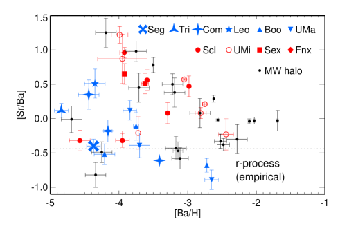
Figure 6: [Sr/Ba] NLTE abundance ratios as a function of [Ba/H]. Stars in Coma Berenices, S40 in Tri ii, and S7 in Seg 1 are shown with four-pointed stars, a three-pointed star, and a cross, respectively. For comparison, we show NLTE abundance ratios from M17b for stars in classical dSphs (circles, squares, diamonds), UFDs (stars, triangles), and the MW halo (small circles). The dashed line indicates the empirical r-process ratio for [Sr/Ba].

Figure 7: The maximal [Sr/Ba] ratios found to date in different dwarf galaxies as a function of fraction of binary stars in the galaxy. See Sect. 5.3 for details.

6 Conclusions

We revisited chemical element abundances of three stars in Coma Berenices UFD, seven stars in Segue 1 UFD, and one star in Tri ii UFD, using high resolution spectral observations from the original papers of Frebel et al. (2010), Frebel et al. (2014), Norris et al. (2010), and Kirby et al. (2017). Our study took advantage of new photometric observations in the visible and infra-red bands obtained with the 2.5 m telescope of the SAI MSU Caucasian observatory and chemical abundance determinations taking into account NLTE effects. The procedure of photometric observations and data reduction was tested, and high data accuracy for faint objects was achieved. The errors in the derived magnitudes are within 0.03 mag.

We determined atmospheric parameters and abundances for up to eighteen chemical elements from carbon to barium in the sample stars. For the first time, we present abundance determination of oxygen in Seg 1 S1 and S4, silicon in ComaBer S2 and Tri ii S40, potassium in Seg 1 S1$-$S6 and ComaBer S1$-$S3, and barium in Seg 1 S7. Our conclusions can be summarized as follows.

• In Segue 1 and Coma Berenices, different stars show different chemical element abundance patterns, which argues for stochastic star formation and incomplete gas mixing in these UFDs. This is in line with the earlier findings of Frebel et al. (2010) and Frebel et al. (2014).

• In each galaxy, we found stars with low [Na/Mg] of $-1.1$ dex. Coma Berenices S2 shows extremely low [Na/Mg] = $-1.68$, which is the lowest value known to date. We interpret this chemical property as a footprint of nucleosynthesis in Pop iii stars. This odd-even effect was not blurred due to a small number of nucleosynthesis events that contributed to chemical abundances of the sample stars.

• We increased the statistics of homogeneous data on Sr and Ba NLTE abundances in UFDs. Our results for Coma Berenices, Segue 1, and Triangulum ii stars confirm that ultra-faint dwarf galaxies are distinct from massive galaxies in Sr production: their [Sr/H] is nearly 1 dex lower, while [Ba/H] is similar (Mashonkina et al., 2017b; Ji et al., 2019). However, in UFDs, just as in massive galaxies, [Sr/Ba] is not constant and it can be higher than the pure r-process ratio, but not as high as in massive galaxies.

• We propose that the additional Sr production at the earliest epoch of galactic formation could be attributed to evolution of massive metal-poor binaries.

Acknowledgments. The authors acknowledge the support from the Program of development of M.V. Lomonosov Moscow State University (Leading Scientific School ”Physics of stars, relativistic objects and galaxies”). T.S., L.M., and P.J. are indebted to the International Space Science Institute (ISSI), Bern, Switzerland, for supporting and funding the international team ”The Pristine” and to the ”ChETEC” COST Action (CA16117), supported by COST (European Cooperation in Science and Technology). T.S. and M.N. are grateful to Foundation for the Advancement of Theoretical Physics and Mathematics ’BASIS’ for financial support (20-1-3-10-1). T.S. is grateful to K. Plotnikov for language editing support. A.F. acknowledge support from NSF grant AST-1716251 and thanks the Wissenschaftskolleg zu Berlin for their wonderful Fellow’s program and generous hospitality. This study is based on spectral observations retrieved from the Keck Observatory Archive (C168Hr), which is operated by the W. M. Keck Observatory and the NASA Exoplanet Science Institute (NExScI), under contract with the National Aeronautics and Space Administration. We made use of the StarFit database http://starfit.org/, SAGA database http://sagadatabase.jp/, the SIMBAD database, operated at CDS, Strasbourg, France; NASA/IPAC Infrared Science Archive, which is operated by the Jet Propulsion Laboratory, California Institute of Technology, under contract with the National Aeronautics and Space Administration; MARCS; and VALD databases. We also thank the referee for useful comments and suggestions.

7 Data availability

The data used in this article will be shared on request to the corresponding author.

8 Appendix

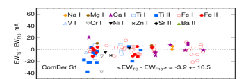
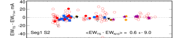
Figure 8: Differences in equivalent width (EW) between this study (TS) and the literature data. For each star, the average difference in EW between TS and the literature data is indicated.

For some stars, we adopted archival spectra, reduced in a different manner, compared to the original papers. Thus, for comparison, we measured the equivalent widths (EWs) and presented a comparison with the original papers. For EW measurements, we apply the following procedure. We fit the synthetic spectrum to the observed spectrum and measure the equivalent width of the synthetic line profile. Figure 8 shows the differences in the equivalent widths between this study and the literature data (Frebel et al., 2010; Frebel et al., 2014; Kirby et al., 2017; Norris et al., 2010). We found a reasonable agreement with the literature data, and, for each star, the average difference in equivalent widths does not exceed the standard deviation. The brighter star, the smaller the scatter in the equivalent width measurements. A large discrepancy of 38 mÅ, was found for the Ti ii 4399 Å and Cr i 4646 Å lines in ComaBer S1 star. This difference is caused by a lower signal to noise ratio in the blue spectrum region. We also note a large difference between this study and K17 found for Sr ii 4077 and 4215Å lines in Tri ii S40. Each of these lines is displaced at the edge of the echelle order, and the uncertainty in accounting for the scattered light can be the source of discrepancies in EWs. Our EWs are smaller and lead to consistent strontium abundance, while, using EWs from K17, leads to a discrepancy of 0.4 dex between the two lines.

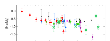
Figure 10: The NLTE chemical abundance ratios for odd-Z elements in different galaxies. Some stars have significantly lower [El/Mg] compared to the mean value.

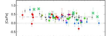
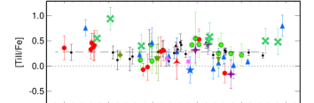
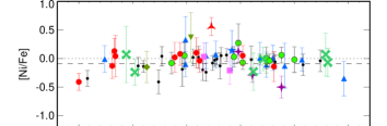
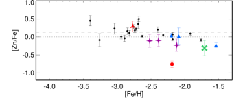
Figure 11: The NLTE chemical abundance ratios in different galaxies. Mean abundance ratios calculated for the MW halo stars are shown with dashed lines. For [Ni/Fe], LTE abundance from Ni i relative to LTE abundance from Fe i is plotted. [$\alpha$/Fe] ratios are high in all Seg 1 stars.

References

- Adelman-McCarthy (2009) Adelman-McCarthy J. K., 2009, VizieR Online Data Catalog, p. II/294
- Alexeeva & Mashonkina (2015) Alexeeva S. A., Mashonkina L. I., 2015, MNRAS, 453, 1619
- Alexeeva et al. (2014) Alexeeva S. A., Pakhomov Y. V., Mashonkina L. I., 2014, Astronomy Letters, 40, 406
- Alonso et al. (1999) Alonso A., Arribas S., Martínez-Roger C., 1999, A&AS, 140, 261
- Andrievsky et al. (2011) Andrievsky S. M., Spite F., Korotin S. A., François P., Spite M., Bonifacio P., Cayrel R., Hill V., 2011, A&A, 530, A105
- Arlandini et al. (1999) Arlandini C., Käppeler F., Wisshak K., Gallino R., Lugaro M., Busso M., Straniero O., 1999, ApJ, 525, 886
- Barklem et al. (2010) Barklem P. S., Belyaev A. K., Dickinson A. S., Gadéa F. X., 2010, A&A, 519, A20
- Barklem et al. (2012) Barklem P. S., Belyaev A. K., Spielfiedel A., Guitou M., Feautrier N., 2012, A&A, 541, A80
- Barklem et al. (2005) Barklem P. S., Christlieb N., Beers T. C., Hill V., Bessell M. S., Holmberg J., Marsteller B., Rossi S., Zickgraf F.-J., Reimers D., 2005, A&A, 439, 129
- Baumueller & Gehren (1996) Baumueller D., Gehren T., 1996, A&A, 307, 961
- Belokurov et al. (2007) Belokurov V., Zucker D. B., Evans N. W., Kleyna J. T., Koposov S., Hodgkin S. T., Irwin M. J., Gilmore G., Wilkinson M. I., Fellhauer M., Bramich D. M., 2007, ApJ, 654, 897
- Belyaev (2013) Belyaev A. K., 2013, A&A, 560, A60
- Belyaev et al. (2018) Belyaev A. K., Voronov Y. V., Gadéa F. X., 2018, ApJ, 867, 87
- Belyaev et al. (2019) Belyaev A. K., Voronov Y. V., Mitrushchenkov A., Guitou M., Feautrier N., 2019, MNRAS, 487, 5097
- Belyaev et al. (2017) Belyaev A. K., Voronov Y. V., Yakovleva S. A., Mitrushchenkov A., Guitou M., Feautrier N., 2017, ApJ, 851, 59
- Belyaev & Yakovleva (2018) Belyaev A. K., Yakovleva S. A., 2018, MNRAS, 478, 3952
- Belyaev et al. (2014) Belyaev A. K., Yakovleva S. A., Barklem P. S., 2014, A&A, 572, A103
- Belyakova & Mashonkina (1997) Belyakova E. V., Mashonkina L. I., 1997, Astronomy Reports, 41, 530
- Bergemann (2011) Bergemann M., 2011, MNRAS, 413, 2184
- Bergemann & Cescutti (2010) Bergemann M., Cescutti G., 2010, A&A, 522, A9
- Bergemann et al. (2019) Bergemann M., Gallagher A. J., Eitner P., Bautista M., Collet R., Yakovleva S. A., Mayriedl A., Plez B., Carlsson M., Leenaarts J., Belyaev A. K., Hansen C., 2019, A&A, 631, A80
- Bergemann & Gehren (2008) Bergemann M., Gehren T., 2008, A&A, 492, 823
- Bergemann et al. (2010) Bergemann M., Pickering J. C., Gehren T., 2010, MNRAS, 401, 1334
- Bertin & Arnouts (1996) Bertin E., Arnouts S., 1996, A&AS, 117, 393
- Bruls (1993) Bruls J. H. M. J., 1993, A&A, 269, 509
- Butler & Giddings (1985) Butler K., Giddings J., 1985, Newsletter on the analysis of astronomical spectra, No. 9, University of London
- Casagrande & VandenBerg (2014) Casagrande L., VandenBerg D. A., 2014, MNRAS, 444, 392
- Cayrel et al. (2004) Cayrel R., Depagne E., Spite M., Hill V., Spite F., François P., Plez B., Beers T., Primas F., Andersen J., Barbuy B., Bonifacio P., 2004, A&A, 416, 1117
- Cescutti et al. (2013) Cescutti G., Chiappini C., Hirschi R., Meynet G., Frischknecht U., 2013, A&A, 553, A51
- Chiaki & Tominaga (2020) Chiaki G., Tominaga N., 2020, arXiv e-prints, p. arXiv:2008.01259
- Chiti et al. (2020) Chiti A., Frebel A., Simon J. D., Erkal D., Chang L. J., Necib L., Ji A. P., Jerjen H., Kim D., Norris J. E., 2020, arXiv e-prints, p. arXiv:2012.02309
- Clem & Landolt (2013) Clem J. L., Landolt A. U., 2013, AJ, 146, 88
- Cohen et al. (2008) Cohen J. G., Christlieb N., McWilliam A., Shectman S., Thompson I., Melendez J., Wisotzki L., Reimers D., 2008, ApJ, 672, 320
- Cohen & Huang (2009) Cohen J. G., Huang W., 2009, ApJ, 701, 1053
- Cohen & Huang (2010) Cohen J. G., Huang W., 2010, ApJ, 719, 931
- Curtis et al. (2019) Curtis S., Ebinger K., Fröhlich C., Hempel M., Perego A., Liebendörfer M., Thielemann F.-K., 2019, ApJ, 870, 2
- Cutri et al. (2003) Cutri R. M., Skrutskie M. F., van Dyk S., Beichman C. A., Carpenter J. M., Chester T., Cambresy L., Evans T., 2003, VizieR Online Data Catalog, p. II/246
- Depagne et al. (2002) Depagne E., Hill V., Spite M., Spite F., Plez B., Beers T. C., Barbuy B., Cayrel R., Andersen J., Bonifacio P., François P., Nordström B., Primas F., 2002, A&A, 390, 187
- Drawin (1968) Drawin H. W., 1968, Zeitschrift für Physik, 211, 404
- François et al. (2007) François P., Depagne E., Hill V., Spite M., Spite F., Plez B., Beers T. C., Andersen J., James G., Barbuy B., Cayrel R., Bonifacio P., Molaro P., Nordström B., Primas F., 2007, A&A, 476, 935
- François et al. (2016) François P., Monaco L., Bonifacio P., Moni Bidin C., Geisler D., Sbordone L., 2016, A&A, 588, A7
- Frebel (2010) Frebel A., 2010, Astronomische Nachrichten, 331, 474
- Frebel & Bromm (2012) Frebel A., Bromm V., 2012, ApJ, 759, 115
- Frebel et al. (2013) Frebel A., Casey A. R., Jacobson H. R., Yu Q., 2013, ApJ, 769, 57
- Frebel et al. (2008) Frebel A., Collet R., Eriksson K., Christlieb N., Aoki W., 2008, ApJ, 684, 588
- Frebel et al. (2019) Frebel A., Ji A. P., Ezzeddine R., Hansen T. T., Chiti A., Thompson I. B., Merle T., 2019, ApJ, 871, 146
- Frebel et al. (2010) Frebel A., Simon J. D., Geha M., Willman B., 2010, ApJ, 708, 560
- Frebel et al. (2014) Frebel A., Simon J. D., Kirby E. N., 2014, ApJ, 786, 74
- Fuhr et al. (1988) Fuhr J. R., Martin G. A., Wiese W. L., 1988, Journal of Physical and Chemical Reference Data, 17
- Fulbright et al. (2004) Fulbright J. P., Rich R. M., Castro S., 2004, ApJ, 612, 447
- Geha et al. (2013) Geha M., Brown T. M., Tumlinson J., Kalirai J. S., Simon J. D., Kirby E. N., VandenBerg D. A., Muñoz R. R., Avila R. J., Guhathakurta P., Ferguson H. C., 2013, ApJ, 771, 29
- Geha et al. (2009) Geha M., Willman B., Simon J. D., Strigari L. E., Kirby E. N., Law D. R., Strader J., 2009, ApJ, 692, 1464
- Gilmore et al. (2013) Gilmore G., Norris J. E., Monaco L., Yong D., Wyse R. F. G., Geisler D., 2013, ApJ, 763, 61
- Grevesse et al. (1996) Grevesse N., Noels A., Sauval A. J., 1996, in Holt S. S., Sonneborn G., eds, Cosmic Abundances Vol. 99 of Astronomical Society of the Pacific Conference Series, Standard Abundances. p. 117
- Gustafsson et al. (2008) Gustafsson B., Edvardsson B., Eriksson K., Jørgensen U. G., Nordlund Å., Plez B., 2008, A&A, 486, 951
- Hansen et al. (2020) Hansen C. J., Koch A., Mashonkina L., Magg M., Bergemann M., Sitnova T., Gallagher A. J., Ilyin I., Caffau E., Zhang H. W., Strassmeier K. G., Klessen R. S., 2020, A&A, 643, A49
- Hansen et al. (2020) Hansen T. T., Marshall J. L., Simon J. D., Li T. S., Bernstein R. A., Pace A. B., Ferguson P., Nagasawa D. Q., Kuehn K., Carollo D., Geha M., James D., Walker A., Diehl H. T., Aguena M., Allam S., Avila S., Bertin E., 2020, ApJ, 897, 183
- Hansen et al. (2017) Hansen T. T., Simon J. D., Marshall J. L., Li T. S., Carollo D., DePoy D. L., Nagasawa D. Q., Bernstein R. A., Drlica-Wagner A., 2017, ApJ, 838, 44
- Heger & Woosley (2010) Heger A., Woosley S. E., 2010, ApJ, 724, 341
- Honda et al. (2004) Honda S., Aoki W., Kajino T., Ando H., Beers T. C., Izumiura H., Sadakane K., Takada-Hidai M., 2004, ApJ, 607, 474
- Ivans et al. (2003) Ivans I. I., Sneden C., James C. R., Preston G. W., Fulbright J. P., Höflich P. A., Carney B. W., Wheeler J. C., 2003, ApJ, 592, 906
- Jablonka et al. (2015) Jablonka P., North P., Mashonkina L., Hill V., Revaz Y., Shetrone M., Starkenburg E., Irwin M., Tolstoy E., Battaglia G., Venn K., Helmi A., Primas F., François P., 2015, A&A, 583, A67
- Ji et al. (2016a) Ji A. P., Frebel A., Ezzeddine R., Casey A. R., 2016a, ApJ, 832, L3
- Ji et al. (2016b) Ji A. P., Frebel A., Simon J. D., Chiti A., 2016b, ApJ, 830, 93
- Ji et al. (2016c) Ji A. P., Frebel A., Simon J. D., Geha M., 2016c, ApJ, 817, 41
- Ji et al. (2019) Ji A. P., Simon J. D., Frebel A., Venn K. A., Hansen T. T., 2019, ApJ, 870, 83
- Jordi et al. (2006) Jordi K., Grebel E. K., Ammon K., 2006, A&A, 460, 339
- Keller et al. (2014) Keller S. C., Bessell M. S., Frebel A., Casey A. R., Asplund M., Jacobson H. R., Lind K., Norris J. E., Yong D., Heger A., Magic Z., da Costa G. S., Schmidt B. P., Tisserand P., 2014, Nature, 506, 463
- Kirby et al. (2017) Kirby E. N., Cohen J. G., Simon J. D., Guhathakurta P., Thygesen A. O., Duggan G. E., 2017, ApJ, 838, 83
- Kobayashi et al. (2020) Kobayashi C., Leung S.-C., Nomoto K., 2020, ApJ, 895, 138
- Kobayashi et al. (2006) Kobayashi C., Umeda H., Nomoto K., Tominaga N., Ohkubo T., 2006, ApJ, 653, 1145
- Koch et al. (2013) Koch A., Feltzing S., Adén D., Matteucci F., 2013, A&A, 554, A5
- Koch et al. (2008) Koch A., Grebel E. K., Gilmore G. F., Wyse R. F. G., Kleyna J. T., Harbeck D. R., Wilkinson M. I., Evans N. W., 2008, AJ, 135, 1580
- Koch et al. (2008) Koch A., McWilliam A., Grebel E. K., Zucker D. B., Belokurov V., 2008, ApJ, 688, L13
- Koch & Rich (2014) Koch A., Rich R. M., 2014, ApJ, 794, 89
- Kornilov et al. (2014) Kornilov V., Safonov B., Kornilov M., Shatsky N., Voziakova O., Potanin S., Gorbunov I., Senik V., Cheryasov D., 2014, PASP, 126, 482
- Laevens et al. (2015) Laevens B. P. M., Martin N. F., Ibata R. A., Rix H.-W., Bernard E. J., Bell E. F., Sesar B., Ferguson A. M. N., Schlafly E. F., Slater C. T., Burgett W. S., 2015, ApJ, 802, L18
- Landolt & Clem (2013) Landolt A. U., Clem J. L., , 2013, Faint UBVRI Photometric Standard Star Fields: KPNO, NOAO Proposal
- Lang et al. (2010) Lang D., Hogg D. W., Mierle K., Blanton M., Roweis S., 2010, AJ, 139, 1782
- Lasker et al. (2008) Lasker B. M., Lattanzi M. G., McLean B. J., Bucciarelli B., Drimmel R., Garcia J., Greene G., Guglielmetti F., Hanley C., Hawkins G., Laidler V. G., 2008, AJ, 136, 735
- Lawler et al. (2019) Lawler J. E., Hala Sneden C., Nave G., Wood M. P., Cowan J. J., 2019, ApJS, 241, 21
- Lawler et al. (2015) Lawler J. E., Sneden C., Cowan J. J., 2015, ApJS, 220, 13
- Lawler et al. (2014) Lawler J. E., Wood M. P., Den Hartog E. A., Feigenson T., Sneden C., Cowan J. J., 2014, ApJS, 215, 20
- Lee et al. (2013) Lee D. M., Johnston K. V., Tumlinson J., Sen B., Simon J. D., 2013, ApJ, 774, 103
- Leggett et al. (2006) Leggett S. K., Currie M. J., Varricatt W. P., Hawarden T. G., Adamson A. J., Buckle J., Carroll T., Davies J. K., Davis C. J., Kerr T. H., Kuhn O. P., Seigar M. S., Wold T., 2006, MNRAS, 373, 781
- Li et al. (2018) Li T. S., Simon J. D., Kuehn K., Pace A. B., Erkal D., Bechtol K., Yanny B., Drlica-Wagner A., Marshall J. L., Lidman C., 2018, ApJ, 866, 22
- Limongi & Chieffi (2012) Limongi M., Chieffi A., 2012, ApJS, 199, 38
- Lodders et al. (2009) Lodders K., Palme H., Gail H.-P., 2009, Landolt Börnstein
- Magg et al. (2020) Magg M., Nordlander T., Glover S. C. O., Hansen C. J., Ishigaki M., Heger A., Klessen R. S., Kobayashi C., Nomoto K., 2020, MNRAS, 498, 3703
- Mannucci et al. (2006) Mannucci F., Della Valle M., Panagia N., 2006, MNRAS, 370, 773
- Martin et al. (2008) Martin N. F., de Jong J. T. A., Rix H.-W., 2008, ApJ, 684, 1075
- Martin et al. (2016) Martin N. F., Ibata R. A., Collins M. L. M., Rich R. M., Bell E. F., Ferguson A. M. N., Laevens B. P. M., Rix H.-W., Chapman S. C., Koch A., 2016, ApJ, 818, 40
- Martinez et al. (2011) Martinez G. D., Minor Q. E., Bullock J., Kaplinghat M., Simon J. D., Geha M., 2011, The Astrophysical Journal, 738, 55
- Mashonkina (2013) Mashonkina L., 2013, A&A, 550, A28
- Mashonkina (2020) Mashonkina L., 2020, MNRAS, 493, 6095
- Mashonkina et al. (1999) Mashonkina L., Gehren T., Bikmaev I., 1999, A&A, 343, 519
- Mashonkina et al. (2011) Mashonkina L., Gehren T., Shi J.-R., Korn A. J., Grupp F., 2011, A&A, 528, A87
- Mashonkina et al. (2017a) Mashonkina L., Jablonka P., Pakhomov Y., Sitnova T., North P., 2017a, A&A, 604, A129
- Mashonkina et al. (2017b) Mashonkina L., Jablonka P., Sitnova T., Pakhomov Y., North P., 2017b, A&A, 608, A89
- Mashonkina et al. (2007) Mashonkina L., Korn A. J., Przybilla N., 2007, A&A, 461, 261
- Mashonkina et al. (2019) Mashonkina L., Sitnova T., Yakovleva S. A., Belyaev A. K., 2019, A&A, 631, A43
- McConnachie & Venn (2020) McConnachie A. W., Venn K. A., 2020, arXiv e-prints, p. arXiv:2007.05011
- Minor (2013) Minor Q. E., 2013, ApJ, 779, 116
- Minor et al. (2019) Minor Q. E., Pace A. B., Marshall J. L., Strigari L. E., 2019, MNRAS, 487, 2961
- Nadjip et al. (2017) Nadjip A. E., Tatarnikov A. M., Toomey D. W., Shatsky N. I., Cherepashchuk A. M., Lamzin S. A., Belinski A. A., 2017, Astrophysical Bulletin, 72, 349
- Nagasawa et al. (2018) Nagasawa D. Q., Marshall J. L., Li T. S., Hansen T. T., Simon J. D., Bernstein R. A., Balbinot E., Drlica-Wagner A., Pace A. B., 2018, ApJ, 852, 99
- Neretina et al. (2020) Neretina M. D., Mashonkina L. I., Sitnova T. M., Yakovleva S. A., Belyaev A. K., 2020, Astronomy Letters, 46, 621
- Niederste-Ostholt et al. (2009) Niederste-Ostholt M., Belokurov V., Evans N. W., Gilmore G., Wyse R. F. G., Norris J. E., 2009, MNRAS, 398, 1771
- Nishimura et al. (2017) Nishimura N., Sawai H., Takiwaki T., Yamada S., Thielemann F.-K., 2017, ApJ, 836, L21
- Nomoto et al. (2013) Nomoto K., Kobayashi C., Tominaga N., 2013, ARA&A, 51, 457
- Nomoto et al. (2006) Nomoto K., Tominaga N., Umeda H., Kobayashi C., Maeda K., 2006, Nuclear Physics A, 777, 424
- Norris et al. (2010) Norris J. E., Gilmore G., Wyse R. F. G., Yong D., Frebel A., 2010, ApJ, 722, L104
- Norris et al. (2013) Norris J. E., Yong D., Bessell M. S., Christlieb N., Asplund M., Gilmore G., Wyse R. F. G., Beers T. C., Barklem P. S., Frebel A., Ryan S. G., 2013, ApJ, 762, 28
- Okamoto et al. (2008) Okamoto S., Arimoto N., Yamada Y., Onodera M., 2008, A&A, 487, 103
- Okamoto et al. (2012) Okamoto S., Arimoto N., Yamada Y., Onodera M., 2012, ApJ, 744, 96
- Ou et al. (2020) Ou X., Roederer I. U., Sneden C., Cowan J. J., Lawler J. E., Shectman S. A., Thompson I. B., 2020, ApJ, 900, 106
- Pakhomov et al. (2019) Pakhomov Y. V., Mashonkina L. I., Sitnova T. M., Jablonka P., 2019, Astronomy Letters, 45, 259
- Pakhomov et al. (2019) Pakhomov Y. V., Ryabchikova T. A., Piskunov N. E., 2019, Astronomy Reports, 63, 1010
- Placco et al. (2015) Placco V. M., Frebel A., Lee Y. S., Jacobson H. R., Beers T. C., Pena J. M., Chan C., Heger A., 2015, ApJ, 809, 136
- Raassen et al. (1998) Raassen A. J. J., Pickering J. C., Uylings P. H. M., 1998, A&AS, 130, 541
- Ramírez & Meléndez (2005) Ramírez I., Meléndez J., 2005, ApJ, 626, 465
- Reichert et al. (2020) Reichert M., Hansen C. J., Hanke M., Skúladóttir Á., Arcones A., Grebel E. K., 2020, A&A, 641, A127
- Rizzuti et al. (2021) Rizzuti F., Cescutti G., Matteucci F., Chieffi A., Hirschi R., Limongi M., Saro A., , 2021, Constraints on stellar rotation from the evolution of Sr and Ba in the Galactic halo
- Roederer (2017) Roederer I. U., 2017, ApJ, 835, 23
- Roederer et al. (2016) Roederer I. U., Mateo M., Bailey John I. I., Song Y., Bell E. F., Crane J. D., Loebman S., Nidever D. L., Olszewski E. W., Shectman S. A., Thompson I. B., Valluri M., Walker M. G., 2016, AJ, 151, 82
- Ruiter et al. (2010) Ruiter A. J., Belczynski K., Sim S. A., Hillebrand t W., Fink M., Kromer M., 2010, in Kalogera V., van der Sluys M., eds, American Institute of Physics Conference Series Vol. 1314 of American Institute of Physics Conference Series, Type Ia Supernovae and Accretion Induced Collapse. pp 233–238
- Ryabchikova et al. (2015) Ryabchikova T., Piskunov N., Kurucz R. L., Stempels H. C., Heiter U., Pakhomov Y., Barklem P. S., 2015, Phys. Scr, 90, 054005
- Schlegel et al. (1998) Schlegel D. J., Finkbeiner D. P., Davis M., 1998, ApJ, 500, 525
- Shetrone et al. (1998) Shetrone M. D., Bolte M., Stetson P. B., 1998, AJ, 115, 1888
- Simon (2019) Simon J. D., 2019, ARA&A, 57, 375
- Simon et al. (2010) Simon J. D., Frebel A., McWilliam A., Kirby E. N., Thompson I. B., 2010, ApJ, 716, 446
- Simon et al. (2011) Simon J. D., Geha M., Minor Q. E., Martinez G. D., Kirby E. N., Bullock J. S., Kaplinghat M., Strigari L. E., Willman B., Choi P. I., Tollerud E. J., Wolf J., 2011, ApJ, 733, 46
- Sitnova & Mashonkina (2018) Sitnova T. M., Mashonkina L. I., 2018, Astronomy Letters, 44, 411
- Sitnova et al. (2016) Sitnova T. M., Mashonkina L. I., Ryabchikova T. A., 2016, MNRAS, 461, 1000
- Sitnova et al. (2020) Sitnova T. M., Yakovleva S. A., Belyaev A. K., Mashonkina L. I., 2020, Astronomy Letters, 46, 0
- Skrutskie et al. (2006) Skrutskie M. F., Cutri R. M., Stiening R., Weinberg M. D., Schneider S., Carpenter J. M., Beichman C., Capps R., Chester T., Elias J., 2006, AJ, 131, 1163
- Spencer et al. (2018) Spencer M. E., Mateo M., Olszewski E. W., Walker M. G., McConnachie A. W., Kirby E. N., 2018, AJ, 156, 257
- Spencer et al. (2017) Spencer M. E., Mateo M., Walker M. G., Olszewski E. W., McConnachie A. W., Kirby E. N., Koch A., 2017, AJ, 153, 254
- Suda et al. (2017) Suda T., Hidaka J., Aoki W., Katsuta Y., Yamada S., Fujimoto M. Y., Ohtani Y., Masuyama M., Noda K., Wada K., 2017, PASJ, 69, 76
- Suda et al. (2008) Suda T., Katsuta Y., Yamada S., Suwa T., Ishizuka C., Komiya Y., Sorai K., Aikawa M., Fujimoto M. Y., 2008, PASJ, 60, 1159
- Takahashi et al. (2018) Takahashi K., Yoshida T., Umeda H., 2018, ApJ, 857, 111
- Takeda et al. (2005) Takeda Y., Hashimoto O., Taguchi H., Yoshioka K., Takada-Hidai M., Saito Y., Honda S., 2005, PASJ, 57, 751
- Thielemann et al. (2017) Thielemann F.-K., Eichler M., Panov I. V., Wehmeyer B., 2017, Annual Review of Nuclear and Particle Science, 67, 253
- Tolstoy et al. (2009) Tolstoy E., Hill V., Tosi M., 2009, ARA&A, 47, 371
- Tominaga et al. (2007) Tominaga N., Umeda H., Nomoto K., 2007, ApJ, 660, 516
- Tsymbal et al. (2019) Tsymbal V., Ryabchikova T., Sitnova T., 2019, in Romanyuk I. I., Yakunin I. A., Kudryavtsev D. O., eds, Physics of magnetic stars Vol. 518 of Astronomical Society of the Pacific Conference Series, Software for NLTE spectrum fitting. p. 247
- Vargas et al. (2013) Vargas L. C., Geha M., Kirby E. N., Simon J. D., 2013, ApJ, 767, 134
- Venn et al. (2012) Venn K. A., Shetrone M. D., Irwin M. J., Hill V., Jablonka P., Tolstoy E., Lemasle B., Divell M., Starkenburg E., Letarte B., Baldner C., Battaglia G., Helmi A., Kaufer A., Primas F., 2012, ApJ, 751, 102
- Venn et al. (2017) Venn K. A., Starkenburg E., Malo L., Martin N., Laevens B. P. M., 2017, MNRAS, 466, 3741
- Vieytes & Fontenla (2013) Vieytes M. C., Fontenla J. M., 2013, ApJ, 769, 103
- Warner (1968) Warner B., 1968, MNRAS, 140, 53
- Watson et al. (2019) Watson D., Hansen C. J., Selsing J., Koch A., Malesani D. B., Andersen A. C., Fynbo J. P. U., Arcones A., Bauswein A., Covino S., Grado A., Heintz K. E., Hunt L., Kouveliotou C., Leloudas G., Levan A. J., Mazzali P., Pian E., 2019, Nature, 574, 497
- Wood et al. (2014) Wood M. P., Lawler J. E., Den Hartog E. A., Sneden C., Cowan J. J., 2014, ApJS, 214, 18
- Wood et al. (2014) Wood M. P., Lawler J. E., Sneden C., Cowan J. J., 2014, ApJS, 211, 20
- Yakovleva et al. (2019) Yakovleva S. A., Voronov Y. V., Belyaev A. K., 2019, Optics and Spectroscopy, 127, 207
- Yi et al. (2004) Yi S. K., Demarque P., Kim Y.-C., 2004, Ap&SS, 291, 261
- Yong et al. (2013) Yong D., Norris J. E., Bessell M. S., Christlieb N., Asplund M., Beers T. C., Barklem P. S., Frebel A., Ryan S. G., 2013, ApJ, 762, 26
- Zhang et al. (2008) Zhang H. W., Gehren T., Zhao G., 2008, A&A, 481, 489
- Zhao et al. (2016) Zhao G., Mashonkina L., Yan H. L., Alexeeva S., Kobayashi C., Pakhomov Y., Shi J. R., Sitnova T., Tan K. F., Zhang H. W., Zhang J. B., Zhou Z. M., Bolte M., Chen Y. Q., Li X., Liu F., Zhai M., 2016, ApJ, 833, 225