A novel approach for the efficient modeling of material dissolution in electrochemical machining

Abstract. This work presents a novel approach to efficiently model anodic dissolution in electrochemical machining. Earlier modeling approaches employ a strict space discretization of the anodic surface that is associated with a remeshing procedure at every time step. Besides that, the presented model is formulated by means of effective material parameters. Thereby, it allows to use a constant mesh for the entire simulation and, thus, decreases the computational costs. Based on Faraday’s law of electrolysis, an effective dissolution level is introduced, which describes the ratio of a dissolved volume and its corresponding reference volume. This inner variable allows the modeling of the complex dissolution process without the necessity of computationally expensive remeshing by controlling the effective material parameters. Additionally, full coupling of the thermoelectric problem is considered and its linearization and numerical implementation are presented. The model shows good agreement with analytical and experimental validation examples by yielding realistic results. Furthermore, simulations of a pulsed electrochemical machining process yield a process signature of the surface roughness related to the specific accumulated electric charge. The numerical examples confirm the simulation’s computational efficiency and accurate modeling qualities.

Keywords: Anodic dissolution, Electrochemical machining, Finite element method

1 Introduction

In many technical systems, materials with a high mechanical and thermal strength are applied to fulfill the efficiency requirements of individual components. Especially in turbomachinery manufacturing, this poses a challenge for conventional machining processes concerning tool wear and the required geometric tolerances. Hence, processes such as electrochemical machining (ECM), in which the strength of the material does not affect the removal process, are gaining importance (Klocke, Klink et al. [2014]). In ECM, the material removal is based on the principle of electrolysis, caused by an electric current between the tool (cathode) and the workpiece (anode) (see e.g. Hamann and Vielstich [2005]). The electric current is enabled by an electrically conductive fluid called electrolyte (see Fig. 1). This removal mechanism allows an efficient machining of high strength materials such as titanium or nickel-alloys, without the occurrence of stress states within rim zones, due to the lack of mechanical and thermal energy during the process (cf. DeBarr and Oliver [1968], McGeough [1974], Bergs and Harst [2020]).

(a) Illustration ECM (Klocke, Zeis et al. [2014])

(b) Experiment ECM

Figure 1: Illustration and experiment of electrochemical machining.

A challenge in ECM is the complex tool development. ECM is an imaging machining process, where the contour of the tool defines the final shape of the workpiece. However, the local material removal rate highly depends on the electric conductivity of the electrolyte, which itself depends on multiple physical phenomena within the gap, such as the two-phase flow and the local temperature (Klocke and König [2007]). Due to multiphysical coupling (cf. van Tijum and Pajak [2008]), the resulting geometry after ECM is difficult to predict using deterministic calculations. In the past, ECM tools have been developed using heuristic experimental approaches, which employ a time-consuming iterative methodology. Experimental studies may be found in e.g. Hopenfeld and Cole [1969], Cook et al. [1973] and Datta and Landolt [1981].

The precise modeling of machining processes is a challenging topic for modern industries. Furthermore, the accurate prediction of process results enables the reduction of calculation time as well as experimental costs. Initially, Tipton [1964] presents the analytical $\mathrm{cos}\,\theta$ method to compute the equilibrium shape of the work piece. Afterwards, e.g. Hümbs [1975] extends this analytical method to account for unsteady sinking conditions. Moreover, numerous numerical models for ECM have been developed and, therefore, only a brief overview is given in the following. Walsch [1977] presents the first numerical model for the computation of the gap width in ECM. Additional physical aspects, like the effect of the grain size on the performance of ECM, are considered by e.g. Rajurkar and Hewidy [1988]. Furthermore, Hardisty et al. [1993] describe the moving boundary value problem in ECM with a two-dimensional finite element model and, further, Hardisty and Mileham [1999] also extend this model for a parabolic cathode shape. Transport mechanisms are first considered by Deconinck et al. [2012a, b, 2013], who, additionally, use the level set method to describe the anodic surface. Zeis [2015] presents a fully coupled multiphysical model of the ECM process that allows for an automated design using iterative simulations. Finally, the dissolution of multiphase materials is modeled by e.g. Kozak and Zybura-Skrabalak [2016] and Harst [2019]. For a comprehensive overview of the numerical models the reader is kindly referred to e.g. Hinduja and Kunieda [2013], Zeis [2015] and Harst [2019].

Although these approaches have proven to be applicable for the related cases, they are based on complex numerical strategies that require intensive fine-tuning, remeshing and high computational costs. To improve the performance of the simulations, we require more efficient approaches for modeling ECM. Hence, this paper presents a modeling approach for the material dissolution based on the concept of effective physical properties. Moreover, the model avoids remeshing and, thus, allows for the simulation of the entire process with one mesh. In this paper, the authors utilize a transient, electro-thermally coupled finite element formulation to accurately model the principal impacts in ECM and, further, to account for the interaction between the electric and thermal field. So far, experiments failed to prove the necessity of considering thermoelectric effects. Nevertheless, we consider a fully coupled model to maintain generality and flexibility for possible future applications. Early works related to the solution of thermoelectric problems may be found e.g. in Buist [1995] who employ the finite element method (FEM) to investigate the steady-state performance of thermoelectric devices and in Lau and Buist [1997] who study the performance of power generation in thermoelectricity. Other authors, e.g. Antonova and Looman [2005], conduct transient investigations of Peltier cooling devices using finite elements. Furthermore, Pérez-Aparicio et al. [2007] present a nonlinear fully coupled finite element formulation for steady-state thermoelectricity. In Palma et al. [2012], the formulation is extended for dynamic problems using a hyperbolic heat conduction model. Moreover, coupling of thermal and electrical fields with the mechanical field may be found in e.g. Pérez-Aparicio, Palma and Moreno-Navarro [2016] and, additionally, with the magnetic field in Pérez-Aparicio, Palma and Taylor [2016].

Outline of the work.  The effective modeling of the anodic dissolution based on Faraday’s law of electrolysis is discussed in Section 2. Thereafter, in Section 3, the governing balance equations of thermoelectricity, the constitutive laws and the corresponding weak forms are presented. Moreover, Section 4 serves to define a unit cell and to introduce a time and space discretization based on the backward Euler method and the finite element method, respectively. In Sections 5.1 - 5.3, analytical and experimental reference solutions validate the model’s performance. Next, in Section 5.4, the model’s predictive capabilities are investigated for the evolution of the surface texture in a pulsed electrochemical machining process. Finally, Section 6 provides the paper’s conclusion.

Notational conventions.  Italic characters $a$, $A$ denote scalars and zeroth-order tensors, bold-face italic characters $\bm{b}$, $\bm{B}$ denote vectors and first-order tensors and bold-face roman characters $\mathbf{c}$, $\mathbf{C}$ refer to matrices and second-order tensors. The operators ${\rm div}\left(\bullet\right)$ and ${\rm grad}\left(\bullet\right)$ define the divergence and gradient of a quantity with respect to Cartesian coordinates. The transpose of a quantity is defined by $(\bullet)^{\mathrm{T}}$. A dot $\cdot$ defines the single contraction of two tensors. The time derivative of a quantity is defined by $\dot{(\bullet)}$.

2 Homogenized description of the anodic dissolution

The anodic dissolution of an arbitrary metal atom $\mathrm{Me}$ is characterized by the oxidation reaction

$$\mathrm{Me}\longrightarrow\mathrm{Me}^{z+}+z\,\mathrm{e}^{-}$$ (1)

where $\mathrm{e}^{-}$ denotes an electron and $z$ the electrochemical valency, which describes the number of electrons which seperate during the chemical process. At the macroscopic level, Faraday’s law of electrolysis describes the related dissolved volume and reads for a multi-phase material according to Klocke and König [2007]:

$$V_{\mathrm{dis}}=\eta\,\sum_{a}\,\lambda_{a}\,\frac{M_{a}}{F\,\rho_{\textrm{\tiny V}a}\,\sum_{b}\,\nu_{b}\,z_{ab}}\,\,I\,t$$ (2)

In Eq. (2), phase $a$ is defined by the volume fraction $\lambda_{a}$, the molar mass $M_{a}$ and the volume density $\rho_{\textrm{\tiny V}a}$. The dissolution is a result of different reactions $b$ which take place with a probability described by the factor $\nu_{b}$ and an individual electrochemical valency $z_{ab}$. Furthermore, the efficiency $\eta$, Faraday’s constant $F=96485$ $\mathrm{A}\text{\,}\mathrm{s}\text{/}\mathrm{mol}$, the current $I$ and the machining time $t$ are taken into account. Based on the work of Harst [2019], we introduce the effectively dissolved volume $V_{\mathrm{eff}}$ as an experimentally detected material parameter which considers anodic gas evolution as well as additional chemical reactions. Up to now, focusing on the anodic dissolution, chemical reactions at the cathode are neglected. Thus, $V_{\mathrm{eff}}$ describes the incremental dissolved volume $\mathrm{d}V_{\mathrm{dis}}$ per incrementally flown electric charge given by $I\mathrm{d}t$. Accordingly, the infinitesimal dissolved volume per time increment reads

$$\dfrac{\mathrm{d}V_{\mathrm{dis}}}{\mathrm{d}t}=V_{\mathrm{eff}}\,I.$$ (3)

The objective of this work is the presentation of a new modeling approach for the anodic dissolution, which enables a computation of the entire process without remeshing. Hence, we define a dissolution level $d\in[0,1]$ as the ratio of the dissolved volume and the corresponding reference volume, which reads per time increment

$$\dfrac{\mathrm{d}d}{\mathrm{d}t}=\frac{\mathrm{d}V_{\mathrm{dis}}}{\mathrm{d}V\,\mathrm{d}t}=\frac{V_{\mathrm{eff}}\,I(\bm{j},d)}{\mathrm{d}V}$$ (4)

where the scalar electric current $I$ is a function of the electric current density $\bm{j}$ and the dissolution level $d$.

In analogy to damage modeling (see e.g. Brepols et al. [2017, 2020]), where the stiffness of the material degrades when damage evolves, the material parameters of the unit cell in electrochemical machining alter, when electrolyte replaces metal material. Thus, the averaged material parameters $\bar{(\bullet)}$ are defined by the mixture of the metal phases and the electrolyte in dependence of the dissolution level $d$

$$\bar{(\bullet)}=\left(1-d\right)\,\sum_{a}\lambda_{a}\,\,(\bullet)_{a}\,+\,d\,\,(\bullet)_{\mathrm{\scriptscriptstyle EL}}$$ (5)

where $(\bullet)_{a}$ denotes the parameters of phase $a$ and $(\bullet)_{\mathrm{\scriptscriptstyle EL}}$ those of the electrolyte, respectively. Moreover, the contact of metal to electrolyte is a mandatory requirement for the chemical process. We, thus, define an activation function $\mathcal{A}$:

$$\mathcal{A}\left(\bm{x},t\right)=\begin{cases}1,&\textrm{contact metal-electrolyte}\\ 0,&\mathrm{else}\end{cases}$$ (6)

The function is active at the position $\bm{x}$, i.e. equal to $1$, if at this point the material consists of a metal phase ($d<1$) and has contact with the electrolyte. Due to the process related replacement of the metal by the electrolyte, the activation function is also evolving in time.

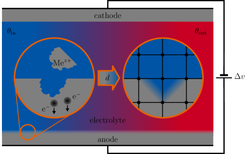
Figure 2: Illustration of anodic dissolution during ECM: chemical process (left), effective description using the dissolution level $d$ (right).

3 Electro-thermal coupling

In thermoelectricity, the constitutively independent variables are the electric potential $v$ and the absolute temperature $\theta$. In the following, all the material parameters denoted with a bar refer to the effective quantities. As described before, they are a result of the phase-electrolyte mixture and can be calculated using Equation (5). The first governing balance equation is the conservation of electric charge (cf. Jackson [1962]):

$$\dot{\rho}_{\textrm{\tiny E}}+{\rm div}\left(\bm{j}\right) =0\hskip 25.89201pt\mathrm{in}\,\,\Omega$$

$$v =\widetilde{v}\hskip 25.60747pt\mathrm{on}\,\,\Gamma_{v}$$ (7)

$$\bm{j}\cdot\bm{n} =\widetilde{j}\hskip 26.17651pt\mathrm{on}\,\,\Gamma_{j}$$

Here, the electric field strength $\bm{E}$ reads

$$\bm{E}=-{\rm grad}\left(v\right),$$ (8)

and the constitutive law of the electric displacement field $\bm{D}$ reads in accordance with the Maxwell equations

$$\bm{D}=\epsilon_{\mathrm{0}}\bar{\epsilon}_{\mathrm{r}}\,\bm{E},$$ (9)

where $\epsilon_{\mathrm{0}}$ and $\bar{\epsilon}_{\mathrm{r}}$ denote the electric constant and the effective relative permittivity, respectively. Moreover, the electric volume charge density $\rho_{\textrm{\tiny E}}$ is defined as

$$\rho_{\textrm{\tiny E}}={\rm div}\left(\bm{D}\right).$$ (10)

Furthermore, the constitutive law of the electric current density $\bm{j}$ consists of three components: the first, related to Ohm’s law $\bm{j}_{\textrm{\tiny L}}$; the second, related to the displacement current $\bm{j}_{\textrm{\tiny V}}$; the third, related to the Seebeck effect $\bm{j}_{\textrm{\tiny S}}$. Thus, the electric current density reads

$$\bm{j}\left(v,\dot{v},\theta\right)=\bm{j}_{\textrm{\tiny L}}\left(v\right)+\bm{j}_{\textrm{\tiny V}}\left(\dot{v}\right)+\bm{j}_{\textrm{\tiny S}}\left(\theta\right)$$ (11)

with the definitions

$$\bm{j}_{\textrm{\tiny L}} \mathrel{\leavevmode\resizebox{0.0pt}{0.0pt}{ $\!\!\leavevmode\resizebox{1.2pt}{0.8pt}{\raisebox{0.99025pt}{$\mathop{:}$}}\!\!=\!\!$ }}\bar{k}_{\textrm{\tiny E}}\left(-{\rm grad}\left(v\right)\right)=\bar{k}_{\textrm{\tiny E}}\,\bm{E},$$ (12)

$$\bm{j}_{\textrm{\tiny V}} \mathrel{\leavevmode\resizebox{0.0pt}{0.0pt}{ $\!\!\leavevmode\resizebox{1.2pt}{0.8pt}{\raisebox{0.99025pt}{$\mathop{:}$}}\!\!=\!\!$ }}\epsilon_{\mathrm{0}}\bar{\epsilon}_{\mathrm{r}}\left(-{\rm grad}\left(\dot{v}\right)\right)=\epsilon_{\mathrm{0}}\bar{\epsilon}_{\mathrm{r}}\,\dot{\bm{E}},$$ (13)

$$\bm{j}_{\textrm{\tiny S}} \mathrel{\leavevmode\resizebox{0.0pt}{0.0pt}{ $\!\!\leavevmode\resizebox{1.2pt}{0.8pt}{\raisebox{0.99025pt}{$\mathop{:}$}}\!\!=\!\!$ }}\bar{k}_{\textrm{\tiny E}}\bar{\alpha}\left(-{\rm grad}\left(\theta\right)\right)$$ (14)

where $\bar{k}_{\textrm{\tiny E}}$ and $\bar{\alpha}$ denote the effective quantities for the electric conductivity and for the Seebeck coefficient.

The second governing balance equation is the transient heat conduction equation:

$$\bar{\rho}_{\textrm{\tiny V}}\bar{c}_{\theta}\,\dot{\theta}+{\rm div}\left(\bm{q}\right) =\bm{j}\cdot\bm{E}+q^{\ast}\hskip 25.60747pt\mathrm{in}\,\Omega$$

$$\theta =\widetilde{\theta}\hskip 70.56284pt\mathrm{on}\,\Gamma_{\theta}$$ (15)

$$\bm{q}\cdot\bm{n} =\widetilde{q}\hskip 70.56284pt\mathrm{on}\,\Gamma_{q}$$

The term $\bm{j}\cdot\bm{E}$ describes Joule-heating and $q^{\ast}$ additional heat sources. However, additional heat evolution due to e.g. chemical reactions is currently neglected. The effective parameters $\bar{\rho}_{\textrm{\tiny V}}$ and $\bar{c}_{\theta}$ denote the volume density and the specific heat capacity. The constitutive law of the heat flux $\bm{q}$ consists of the part related to the Peltier effect $\bm{q}_{\textrm{\tiny P}}$ and the part related to Fourier’s law $\bm{q}_{\textrm{\tiny F}}$. Hence, the heat flux reads

$$\bm{q}\left(v,\dot{v},\theta\right)=\bm{q}_{\textrm{\tiny P}}\left(v,\dot{v},\theta\right)+\bm{q}_{\textrm{\tiny F}}\left(\theta\right)$$ (16)

with the definitions

$$\bm{q}_{\textrm{\tiny P}} \mathrel{\leavevmode\resizebox{0.0pt}{0.0pt}{ $\!\!\leavevmode\resizebox{1.2pt}{0.8pt}{\raisebox{0.99025pt}{$\mathop{:}$}}\!\!=\!\!$ }}\bar{\Pi}\,\bm{j},$$ (17)

$$\bm{q}_{\textrm{\tiny F}} \mathrel{\leavevmode\resizebox{0.0pt}{0.0pt}{ $\!\!\leavevmode\resizebox{1.2pt}{0.8pt}{\raisebox{0.99025pt}{$\mathop{:}$}}\!\!=\!\!$ }}\bar{k}_{\theta}\left(-{\rm grad}\left(\theta\right)\right)$$ (18)

where $\bar{\Pi}$ and $\bar{k}_{\theta}$ denote the Peltier coefficient and the thermal conductivity, both in their efficient representation. For the non-transient case, an analogous structure of the constitutive equations may be found in e.g. Pérez-Aparicio et al. [2007]. Moreover, Table 1 shows the material parameters’ SI units and definitions. By inserting the constitutive equations into the governing balance equations, multiplying with the arbitrary test functions $\delta v$ and $\delta\theta$ and employing partial integration, the weak forms $g_{v}$ and $g_{\theta}$ are obtained (cf. Pérez-Aparicio et al. [2007], non-transient):

$$g_{v}\mathrel{\leavevmode\resizebox{0.0pt}{0.0pt}{ $\!\!\leavevmode\resizebox{1.2pt}{0.8pt}{\raisebox{0.99025pt}{$\mathop{:}$}}\!\!=\!\!$ }}-\int_{\Omega}\left(\,\bm{j}+\,\bm{j}_{\textrm{\tiny V}}\right)\cdot{\rm grad}\left(\delta v\right)\mathrm{d}V+g_{\tilde{j}}=0$$ (19)

$$g_{\theta}\mathrel{\leavevmode\resizebox{0.0pt}{0.0pt}{ $\!\!\leavevmode\resizebox{1.2pt}{0.8pt}{\raisebox{0.99025pt}{$\mathop{:}$}}\!\!=\!\!$ }}\int_{\Omega}\left(\bar{\rho}_{\textrm{\tiny V}}\bar{c}_{\theta}\dot{\theta}-\bm{j}\cdot\bm{E}-q^{\ast}\right)\delta\theta\,\mathrm{d}V-\int_{\Omega}\bm{q}\cdot{\rm grad}\left(\delta\theta\right)\mathrm{d}V+g_{\tilde{q}}=0$$ (20)

The primary unknowns are the electric potential $v$ and the absolute temperature $\theta$. Furthermore, the dissolution level $d$ deals as an internal variable and, thus, influences the effective material parameters within the weak forms (19) and (20). The quantities $g_{\tilde{j}}$ and $g_{\tilde{q}}$ denote prescribed electric current densities and heat fluxes.

Table 1: Physical constants and material parameters

$\epsilon_{\mathrm{0}}$	$[$\mathrm{A}\text{\,}\mathrm{s}\text{/}\text{(}\mathrm{V}\text{\,}\mathrm{m}\text{)}$]$	Electric constant $\left(8.854\times 10^{-12}\right)$
$F$	$[$\mathrm{A}\text{\,}\mathrm{s}\text{/}\mathrm{mol}$]$	Faraday constant $\left(9.648\times 10^{4}\right)$
$a$	$[-]$	Phase $a$
$b$	$[-]$	Reaction $b$
$\alpha$	$[$\mathrm{V}\text{/}\mathrm{K}$]$	Seebeck coefficient
$\epsilon_{\mathrm{r}}$	$[-]$	Relative permittivity
$\eta$	$[-]$	Efficiency
$\lambda$	$[-]$	Volume fraction
$\nu$	$[-]$	Probability factor
$\Pi$	$[$\mathrm{V}\text{/}{\mathrm{K}}^{2}$]$	Peltier coefficient $(\Pi=\alpha\,\theta)$
$\rho_{\textrm{\tiny V}}$	$[$\mathrm{kg}\text{/}{\mathrm{m}}^{3}$]$	Volume density
$c_{\theta}$	$[$\mathrm{J}\text{/}\text{(}\mathrm{kg}\text{\,}\mathrm{K}\text{)}$]$	Specific heat capacity
$k_{\textrm{\tiny E}}$	$[$\mathrm{A}\text{/}\text{(}\mathrm{V}\text{\,}\mathrm{m}\text{)}$]$	Electric conductivity
$k_{\theta}$	$[$\mathrm{W}\text{/}\text{(}\mathrm{m}\text{\,}\mathrm{K}\text{)}$]$	Thermal conductivity
$M$	$[$\mathrm{kg}\text{/}\mathrm{mol}$]$	Molar mass
$V_{\mathrm{eff}}$	$[${\mathrm{m}}^{3}\text{/}\text{(}\mathrm{A}\text{\,}\mathrm{s}\text{)}$]$	Effectively dissolved volume
$z$	$[-]$	Electrochemical valency

4 Discretization and finite element implementation

4.1 Definition of a unit cell

As written in Eq. (4), the dissolution level per time $\mathrm{d}d/\mathrm{d}t$ describes the ratio of the related dissolved volume increment $\mathrm{d}V_{\mathrm{dis}}$ (see Eq. (3)) per volume and time increment. We employ the concept of a unit cell, and, therefore, the dissolution level $d$ defines the relative dissolved volume of a unit cell. Accordingly, the rate of the dissolution level per unit cell volume reads

$$\dot{d}=\dfrac{1}{V_{\mathrm{uc}}}\dfrac{\mathrm{d}V_{\mathrm{dis}}}{\mathrm{d}t}$$ (21)

and allows a smoother description of the chemical reaction (see Fig. 2) compared to earlier works. The size of the unit cell may be chosen arbitrarily. However, the unknowns, i.e. the volume $V_{\mathrm{uc}}$ and the scalar electric current $I$, must be computed consistently. The vector of the electric current density $\bm{j}$ must be transferred to a scalar electric current $I$, because Faraday’s law of electrolysis is formulated on a scalar basis (see Eq. (2)). Here, in the finite element framework, we define a unit cell at each integration point. The unit cell’s volume $V_{\mathrm{uc}}$ is deduced from the finite element’s volume $V_{\mathrm{el}}$ and the number of integration points $n_{\mathrm{gp}}$

$$V_{\mathrm{uc}}=\frac{V_{\mathrm{el}}}{n_{\mathrm{gp}}}.$$ (22)

Moreover, the areas of the unit cell, that enable the transformation of the three-dimensional electric current density vector to a scalar electric current, are computed analogously from the element’s areas

$$A_{\mathrm{uc}x}=\frac{A_{\mathrm{el}x}}{n_{\mathrm{gp}}},\quad A_{\mathrm{uc}y}=\frac{A_{\mathrm{el}y}}{n_{\mathrm{gp}}},\quad A_{\mathrm{uc}z}=\frac{A_{\mathrm{el}z}}{n_{\mathrm{gp}}}.$$ (23)

Fig. 3 defines the element’s areas $A_{\mathrm{el}x}$, $A_{\mathrm{el}y}$ and $A_{\mathrm{el}z}$ for an arbitrarily shaped element. They are calculated from the intersection points of the element’s edges with the $x$-, $y$- and $z$-plane. The position vector $\bm{x}_{\textrm{\tiny M}}$ in the center of the element and the normals $\bm{n}_{x}$, $\bm{n}_{y}$ and $\bm{n}_{z}$ define these planes.

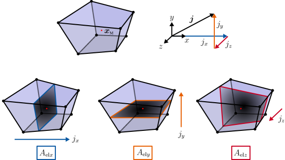
Figure 3: Definition of element areas $A_{\mathrm{el}x}$, $A_{\mathrm{el}y}$ and $A_{\mathrm{el}z}$.

Afterwards, we employ the transfer of the electric current densities and arrange the electric currents in descending order

$$\begin{Bmatrix}\|A_{\mathrm{uc}x}\,j_{x}\|\\ \|A_{\mathrm{uc}y}\,j_{y}\|\\ \|A_{\mathrm{uc}z}\,j_{z}\|\end{Bmatrix}\longmapsto\begin{Bmatrix}I_{1}\\ I_{2}\\ I_{3}\end{Bmatrix},\qquad I_{1}\geq I_{2}\geq I_{3}.$$ (24)

Finally, the evolution equation of the dissolution level $d$ is expressed in terms of $I_{1}$, $I_{2}$ and $I_{3}$. We assume that current $I_{1}$ fully contributes to the evolution of the dissolution. The reduction of $I_{2}$ and $I_{3}$ by the factor $(1-d)$ considers the dissolution level of the element (see Fig. 4) and, hence, reduces the areas of the element and the unit cell. Therefore, the dissolution rate $\dot{d}$ reads

$$\dot{d}=\frac{1}{V_{\mathrm{uc}}}\,V_{\mathrm{eff}}\left[I_{1}+(1-d)\left(I_{2}+I_{3}\right)\right]\mathcal{A}\left(\bm{x},t\right).$$ (25)

The reduction of the electric currents $I_{2}$ and $I_{3}$ aims to avoid an overestimation of the dissolution, since the electric current densities, which pass not perpendicular but parallel to the dissolved volume, just partially contribute to the dissolution (see Fig. 4).

Figure 4: Reduction of the element areas $A_{\mathrm{el}x}$, $A_{\mathrm{el}y}$ and $A_{\mathrm{el}z}$ to take the dissolution level $d$ into account. In this illustration, current $I_{1}$ is assumed in $x$-direction. The volume marked in red denotes the related dissolved volume.

4.2 Time discretization

The backward Euler method serves to obtain the time discretized expression for the dissolution rate $\dot{d}$ from Eq. (25). It reads, under the assumption that the activation function $\mathcal{A}$ is active,

$$\frac{d_{n+1}-d_{n}}{\Delta t}=\frac{1}{V_{\mathrm{uc}}}\,V_{\mathrm{eff}}\left[\left(I_{1}\right)_{n+1}+\left(1-d_{n+1}\right)\left(\left(I_{2}\right)_{n+1}+\left(I_{3}\right)_{n+1}\right)\right]$$ (26)

where $V_{\mathrm{uc}}$ and $V_{\mathrm{eff}}$ are constant over time. Rewriting Eq. (26), an explicit expression for $d_{n+1}$ is obtained

$$d_{n+1}=\frac{d_{n}+\frac{V_{\mathrm{eff}}}{V_{\mathrm{uc}}}\left(\left(I_{1}\right)_{n+1}+\left(I_{2}\right)_{n+1}+\left(I_{3}\right)_{n+1}\right)\Delta t}{1+\frac{V_{\mathrm{eff}}}{V_{\mathrm{uc}}}\left(\left(I_{2}\right)_{n+1}+\left(I_{3}\right)_{n+1}\right)\Delta t}.$$ (27)

If a value $d_{n+1}>1$ is computed, the current value of the dissolution is reset to $d_{n+1}=1$. Analogously, we discretize the time derivatives of the primary variables $v$ and $\theta$ to

$$\big{(}\,\dot{v}\,\big{)}_{n+1}=\frac{v_{n+1}-v_{n}}{\Delta t},\hskip 28.45274pt\big{(}\,\dot{\theta}\,\big{)}_{n+1}=\frac{\theta_{n+1}-\theta_{n}}{\Delta t}.$$ (28)

4.3 Finite element discretization

Considering Eq. (28), Appendix A.1 shows the linearization of the weak forms (Eqs. (19)-(20)) with respect to $v_{n+1}$ and $\theta_{n+1}$. Hereby, the effective material parameters’ dependence on temperature and dissolution is considered in a staggered approach.

We, thus, assume $\bar{(\bullet)}\mathrel{\leavevmode\resizebox{0.0pt}{0.0pt}{ $\!\!\leavevmode\resizebox{1.2pt}{0.8pt}{\raisebox{0.99025pt}{$\mathop{:}$}}\!\!=\!\!$ }}\bar{(\bullet)}\left(d_{n},\theta_{n}\right)$, where $d_{n}$ and $\theta_{n}$ denote the quantities from the previous time step $t_{n}$. Following the linearization, the problem is spatially discretized employing the finite element method. Therefore, the entire domain is subdivided and approximated by finite elements

$$\Omega\approx\bigcup\limits_{e=1}^{n_{\mathrm{el}}}\,\Omega^{e}.$$ (29)

The primary variables and their variations are approximated with standard tri-linear shape functions

$$v\left(\bm{x}\right) \approx v^{e}\left(\bm{x}\right)=\bm{N}_{v}^{e}\left(\bm{x}\right)\,\bm{v}^{e},$$

$$\theta\left(\bm{x}\right) \approx\theta^{e}\left(\bm{x}\right)=\bm{N}_{\theta}^{e}\left(\bm{x}\right)\,\bm{\theta}^{e},$$

$$\delta v\left(\bm{x}\right) \approx\delta v^{e}\left(\bm{x}\right)=\bm{N}_{v}^{e}\left(\bm{x}\right)\,\delta\bm{v}^{e},$$

$$\delta\theta\left(\bm{x}\right) \approx\delta\theta^{e}\left(\bm{x}\right)=\bm{N}_{\theta}^{e}\left(\bm{x}\right)\,\delta\bm{\theta}^{e}$$

$$\bm{x}\in\Omega^{e}$$ (30)

where $\bm{N}_{v}^{e}$ and $\bm{N}_{\theta}^{e}$ (row vectors) contain the shape function values and $\bm{v}^{e}$, $\delta\bm{v}^{e}$, $\bm{\theta}^{e}$ and $\delta\bm{\theta}^{e}$ (column vectors) the element’s nodal values. The spatial derivatives of these quantities are computed accordingly with the shape function’s derivatives that are stored in the matrices $\mathbf{B}_{v}^{e}$ and $\mathbf{B}_{\theta}^{e}$:

$${\rm grad}\left(v\left(\bm{x}\right)\right) \approx{\rm grad}\left(v\left(\bm{x}\right)\right)^{e}=\mathbf{B}_{v}^{e}\left(\bm{x}\right)\,\bm{v}^{e}, {\rm grad}\left(\delta v\left(\bm{x}\right)\right)\approx{\rm grad}\left(\delta v\left(\bm{x}\right)\right)^{e}=\mathbf{B}_{v}^{e}\left(\bm{x}\right)\,\delta\bm{v}^{e},$$

$${\rm grad}\left(\theta\left(\bm{x}\right)\right) \approx{\rm grad}\left(\theta\left(\bm{x}\right)\right)^{e}=\mathbf{B}_{\theta}^{e}\left(\bm{x}\right)\,\bm{\theta}^{e}, {\rm grad}\left(\delta\theta\left(\bm{x}\right)\right)\approx{\rm grad}\left(\delta\theta\left(\bm{x}\right)\right)^{e}=\mathbf{B}_{\theta}^{e}\left(\bm{x}\right)\,\delta\bm{\theta}^{e}\hphantom{,}$$

$$\bm{x}\in\Omega^{e}\hskip 26.46106pt$$ (31)

Afterwards, the previously derived approximations (Eqs. (30)-(31)) are inserted into the linearized weak forms (Eqs. (42)-(43)):

$$\sum_{e=1}^{n_{\mathrm{el}}}\,\delta\bm{v}^{e\mathrm{T}}\,\Big{\{}\left[\,\mathbf{k}_{vv}^{e}+\mathbf{c}_{vv}^{e}\,\right]\,\Delta\bm{v}_{n+1}^{e}+\left[\hskip 15.07996pt\mathbf{k}_{v\theta}^{e}\hskip 17.35619pt\right]\,\Delta\bm{\theta}_{n+1}^{e}\Big{\}}=\sum_{e=1}^{n_{\mathrm{el}}}\,-\,\delta\bm{v}^{e\mathrm{T}}\,\Big{\{}\,\bm{r}_{v}^{e}\,\Big{\}}$$ (32)

$$\sum_{e=1}^{n_{\mathrm{el}}}\,\delta\bm{\theta}^{e\mathrm{T}}\,\Big{\{}\left[\,\mathbf{k}_{\theta v}^{e}+\mathbf{c}_{\theta v}^{e}\,\right]\,\Delta\bm{v}_{n+1}^{e}+\left[\,\mathbf{k}_{\theta\theta}^{e}+\mathbf{c}_{\theta\theta}^{e}\,\right]\,\Delta\bm{\theta}_{n+1}^{e}\Big{\}}=\sum_{e=1}^{n_{\mathrm{el}}}\,-\,\delta\bm{\theta}^{e\mathrm{T}}\,\Big{\{}\,\bm{r}_{\theta}^{e}\,\Big{\}}$$ (33)

Here, contributions from prescribed surface electric current densities and prescribed surface heat fluxes are neglected. Appendix A.2 shows the definition of the matrices $\mathbf{k}_{vv}^{e}$, $\mathbf{k}_{v\theta}^{e}$, $\mathbf{k}_{\theta v}^{e}$, $\mathbf{k}_{\theta\theta}^{e}$, $\mathbf{c}_{vv}^{e}$, $\mathbf{c}_{\theta v}^{e}$ and $\mathbf{c}_{\theta\theta}^{e}$ and of the residual vectors $\bm{r}_{v}^{e}$ and $\bm{r}_{\theta}^{e}$. Finally, the global equation system is assembled by considering the boundary conditions and the arbitrariness of the test functions:

$$\begin{bmatrix}\mathbf{K}_{vv}+\mathbf{C}_{vv}&\mathbf{K}_{v\theta}\\ \mathbf{K}_{\theta v}+\mathbf{C}_{\theta v}&\mathbf{K}_{\theta\theta}+\mathbf{C}_{\theta\theta}\end{bmatrix}\begin{Bmatrix}\Delta\bm{v}_{n+1}\\ \Delta\bm{\theta}_{n+1}\end{Bmatrix}=-\begin{Bmatrix}\bm{R}_{v}\\ \bm{R}_{\theta}\end{Bmatrix}$$ (34)

The increments $\Delta\bm{v}_{n+1}$ and $\Delta\bm{\theta}_{n+1}$ are computed in each global Newton-Raphson iteration and the components of the tangent matrix and the residual vector are assembled according to

$$\mathbf{K}_{vv} =\text{\raisebox{-4.2679pt}{$\overset{n_{\mathrm{el}}}{\underset{e=1}{\textbf{{\LARGE{A}}}}}$}}\left(\mathbf{k}_{vv}^{e}\right),\quad\mathbf{K}_{v\theta}=\text{\raisebox{-4.2679pt}{$\overset{n_{\mathrm{el}}}{\underset{e=1}{\textbf{{\LARGE{A}}}}}$}}\left(\mathbf{k}_{v\theta}^{e}\right),\quad\mathbf{K}_{\theta v}=\text{\raisebox{-4.2679pt}{$\overset{n_{\mathrm{el}}}{\underset{e=1}{\textbf{{\LARGE{A}}}}}$}}\left(\mathbf{k}_{\theta v}^{e}\right),\quad\mathbf{K}_{\theta\theta}=\text{\raisebox{-4.2679pt}{$\overset{n_{\mathrm{el}}}{\underset{e=1}{\textbf{{\LARGE{A}}}}}$}}\left(\mathbf{k}_{\theta\theta}^{e}\right),$$

$$\mathbf{C}_{vv} =\text{\raisebox{-4.2679pt}{$\overset{n_{\mathrm{el}}}{\underset{e=1}{\textbf{{\LARGE{A}}}}}$}}\left(\mathbf{c}_{vv}^{e}\right),\quad\mathbf{C}_{\theta v}=\text{\raisebox{-4.2679pt}{$\overset{n_{\mathrm{el}}}{\underset{e=1}{\textbf{{\LARGE{A}}}}}$}}\left(\mathbf{c}_{\theta v}^{e}\right),\quad\mathbf{C}_{\theta\theta}=\text{\raisebox{-4.2679pt}{$\overset{n_{\mathrm{el}}}{\underset{e=1}{\textbf{{\LARGE{A}}}}}$}}\left(\mathbf{c}_{\theta\theta}^{e}\right),$$ (35)

$$\bm{R}_{v} =\text{\raisebox{-4.2679pt}{$\overset{n_{\mathrm{el}}}{\underset{e=1}{\textbf{{\LARGE{A}}}}}$}}\left(\bm{r}_{v}^{e}\right),\quad\bm{R}_{\theta}=\text{\raisebox{-4.2679pt}{$\overset{n_{\mathrm{el}}}{\underset{e=1}{\textbf{{\LARGE{A}}}}}$}}\left(\bm{r}_{\theta}^{e}\right).$$

For further information on the finite element method, the reader is kindly referred to the literature of e.g. Hughes [1987] and Zienkiewicz et al. [2005].

5 Numerical examples

This section presents the application of the previously developed model in numerical examples. First, we validate the model’s capabilities to accurately model material dissolution by analytical and experimental reference solutions. Then, we apply the model to exemplarily compute a so-called process signature motivated by the work of the transregional Collaborative Research Center 136 “Process Signatures”, see Brinksmeier et al. [2018].

The temperature-dependent material parameters in the following examples are approximated by cubic polynomials

$$f(\theta)=c_{0}+c_{1}\,\theta+c_{2}\,\theta^{2}+c_{3}\,\theta^{3}$$ (36)

where the absolute temperature $\theta$ is given in $[$\mathrm{K}\text{/}$]$ and the coefficients $c_{0}$, $c_{1}$, $c_{2}$ and $c_{3}$ in Table 2. The functions stem from the works of Zeis [2015] and Harst [2019] where they have been identified for a steel 42CrMo4 and an electrolyte solution with $20$ wt.-$\mathrm{\char 37\relax}\text{/}$ NaNO₃. Due to the lack of experimental data, we assume the Seebeck coefficients in the range of water and aluminum to $\alpha^{\textrm{\tiny EL}}=1\,$\mathrm{\SIUnitSymbolMicro V}\text{/}\mathrm{K}$$ and $\alpha^{\textrm{\tiny ME}}=5\,$\mathrm{\SIUnitSymbolMicro V}\text{/}\mathrm{K}$$, where the superscript $(\bullet)^{\textrm{\tiny EL}}$ indicates the reference to the electrolyte and $(\bullet)^{\textrm{\tiny ME}}$ to steel. The following examples neglect fluid mechanical effects. Moreover, we model Joule-heating in the electrolyte by defining the in- and outflow temperature of the electrolyte which is obtained from experimental investigations. The contribution from $\bm{j}\cdot\bm{E}$ is not considered in electrolyte finite elements to avoid an unphysical overheating of the electrolyte, since cooling effects due to flushing are neglected. Future work focuses on the precise modeling of the electrolyte temperature in cooperation with computational fluid dynamical simulations.

Table 2: Coefficients of material parameters

$f(\theta)$	unit	$c_{0}$	$c_{1}$	$c_{2}$	$c_{3}$
$c_{\theta}^{\textrm{\tiny EL}}$	$[$\mathrm{J}\text{/}\text{(}\mathrm{kg}\text{\,}\mathrm{K}\text{)}$]$	$8.145\times 10^{3}$	$-3.204\times 10^{1}$	$8.371\times 10^{-2}$	$-6.979\times 10^{-5}$
$c_{\theta}^{\textrm{\tiny ME}}$	$[$\mathrm{J}\text{/}\text{(}\mathrm{kg}\text{\,}\mathrm{K}\text{)}$]$	$3.554\times 10^{2}$	$2.848\times 10^{-1}$	$-5.000\times 10^{-5}$	$-$
$k_{\textrm{\tiny E}}^{\textrm{\tiny EL}}$	$[$\mathrm{A}\text{/}\text{(}\mathrm{V}\text{\,}\mathrm{m}\text{)}$]$	$-6.302\times 10^{1}$	$2.530\times 10^{-1}$	$-$	$-$
$k_{\textrm{\tiny E}}^{\textrm{\tiny ME}}$	$[$\mathrm{A}\text{/}\text{(}\mathrm{V}\text{\,}\mathrm{m}\text{)}$]$	$1.131\times 10^{7}$	$-3.710\times 10^{4}$	$6.020\times 10^{1}$	$-3.994\times 10^{-2}$
$k_{\theta}^{\textrm{\tiny EL}}$	$[$\mathrm{W}\text{/}\text{(}\mathrm{m}\text{\,}\mathrm{K}\text{)}$]$	$-8.691\times 10^{-1}$	$8.949\times 10^{-3}$	$-1.584\times 10^{-5}$	$7.975\times 10^{-9}$
$k_{\theta}^{\textrm{\tiny ME}}$	$[$\mathrm{W}\text{/}\text{(}\mathrm{m}\text{\,}\mathrm{K}\text{)}$]$	$3.651\times 10^{1}$	$4.899\times 10^{-2}$	$-1.012\times 10^{-4}$	$4.654\times 10^{-8}$
$V_{\mathrm{eff}}^{\textrm{\tiny ME}}$	$[${\mathrm{m}}^{3}\text{/}\text{(}\mathrm{A}\text{\,}\mathrm{s}\text{)}$]$	$3.650\times 10^{-11}$	$-$	$-$	$-$
$\alpha^{\textrm{\tiny EL}}$	$[$\mathrm{V}\text{/}\mathrm{K}$]$	$1.000\times 10^{-6}$	$-$	$-$	$-$
$\alpha^{\textrm{\tiny ME}}$	$[$\mathrm{V}\text{/}\mathrm{K}$]$	$5.000\times 10^{-6}$	$-$	$-$	$-$
$\epsilon_{\mathrm{r}}^{\textrm{\tiny EL}}$	$[-]$	$1.000\times 10^{0}$	$-$	$-$	$-$
$\epsilon_{\mathrm{r}}^{\textrm{\tiny ME}}$	$[-]$	$8.000\times 10^{1}$	$-$	$-$	$-$
$\rho_{\textrm{\tiny V}}^{\textrm{\tiny EL}}$	$[$\mathrm{kg}\text{/}{\mathrm{m}}^{3}$]$	$8.385\times 10^{2}$	$1.401\times 10^{0}$	$3.011\times 10^{-3}$	$3.718\times 10^{-7}$
$\rho_{\textrm{\tiny V}}^{\textrm{\tiny ME}}$	$[$\mathrm{kg}\text{/}{\mathrm{m}}^{3}$]$	$7.849\times 10^{2}$	$-6.289\times 10^{-2}$	$-4.167\times 10^{-4}$	$1.907\times 10^{-7}$

5.1 Stationary dissolution process - analytical validation

The first example considers a stationary dissolution process, i.e. the cathode’s feed rate $\dot{x}_{\mathrm{ca}}$ and the anode’s dissolution rate $\dot{x}_{\mathrm{an}}$ coincide. Fig. 5(a) shows the initial geometrical setup with $l=1\,$\mathrm{mm}\text{/}$$. A thickness of $g=0.1\,$\mathrm{mm}\text{/}$$ is assumed. Klocke and König [2007] derive the formula for the gap width $s$ in the stationary dissolution process according to

$$s=\frac{k_{\textrm{\tiny E}}^{\textrm{\tiny EL}}\left(\Delta v-\Delta v_{\mathrm{pol}}\right)V_{\mathrm{eff}}}{\dot{x}_{\mathrm{ca}}}.$$ (37)

In this example, we strive to compare the numerical results with a simple, analytical reference solution and, therefore, differing from Table 2, set the electrolyte’s electric conductivity to $k_{\textrm{\tiny E}}^{\textrm{\tiny EL}}=16\,$\mathrm{A}\text{/}\text{(}\mathrm{V}\text{\,}\mathrm{m}\text{)}$$ and the effectively dissolved volume to $V_{\mathrm{eff}}^{\textrm{\tiny ME}}=10^{-11}\,${\mathrm{m}}^{3}\text{/}\text{(}\mathrm{A}\text{\,}\mathrm{s}\text{)}$$. The applied voltage is $\Delta v=20\,$\mathrm{V}\text{/}$$, a polarization voltage $\Delta v_{\mathrm{pol}}$ is neglected and the feed rate is $\dot{x}_{\mathrm{ca}}=10^{-5}\,$\mathrm{m}\text{/}\mathrm{s}$$. With these assumptions, the stationary gap width yields $s=0.32\,$\mathrm{mm}\text{/}$$. Additionally, we apply a constant temperature distribution of $\widetilde{\theta}=323.15\,$\mathrm{K}\text{/}$$ to avoid inhomogeneous electric current density distributions due to the Seebeck effect and, thereby, ensure consistency with the one-dimensional analytical reference solution.

(a) Geometry

(b) BVP

Figure 5: Geometry and boundary value problem of the analytical reference solution for the stationary dissolution process.

Fig. 5(b) shows the boundary value problem (BVP). A constant electric potential of $\widetilde{v}_{\mathrm{an}}=20\,$\mathrm{V}\text{/}$$ is applied at $x=0\,$\mathrm{mm}\text{/}$$. To model the cathode’s feed, the electric potential at $x=1.32\,$\mathrm{mm}\text{/}$$ is time varying with an initial value of $\widetilde{v}_{\mathrm{ca}}=0\,$\mathrm{V}\text{/}$$. Under the assumption of a negligible potential drop in the metal and of a linear potential distribution in the electrolyte, we apply the theorem of intersecting lines. Thus, the function for the electric potential at $x=1.32\,$\mathrm{mm}\text{/}$$ reads

$$\widetilde{v}_{\mathrm{ca}}(t)=-\frac{\widetilde{v}_{\mathrm{an}}\,\dot{x}_{\mathrm{ca}}}{s}\,t$$ (38)

and, thereby, ensures that the theoretical position of the cathode’s surface coincides with the position of the electric potential where $v=0\,$\mathrm{V}\text{/}$$ holds (cf. Fig. 6).

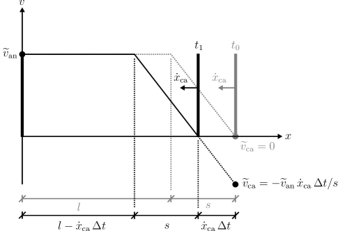
Figure 6: Applying the theorem of intersecting lines to prescribe the electric potential distribution at $t_{0}$ and $t_{1}$ to ensure that the cathode’s position and $v=0$ $\mathrm{V}\text{/}$ coincide.

This example serves to investigate different finite element discretizations. For the coarsest mesh, the workpiece consists of $10\times 10$ elements and for the finest of $80\times 80$ elements. Fig. 7 shows the contour plots of the dissolution level $d$ for a machining time of $0$ $\mathrm{s}\text{/}$, $15$ $\mathrm{s}\text{/}$ and $60$ $\mathrm{s}\text{/}$ for both, the coarsest and finest, meshes with a time increment of $\Delta t=0.01~{}$\mathrm{s}\text{/}$$. A dissolution level of $d=0$ corresponds to pure metal and of $d=1$ to pure electrolyte. The vertical white line visualizes the analytical reference solution after $15$ $\mathrm{s}\text{/}$ and $60$ $\mathrm{s}\text{/}$. The results of both meshes show good agreement with the analytical reference solution. However, the coarsest mesh overestimates the dissolution at $t=60$ $\mathrm{s}\text{/}$ by $+\,5.4~{}$\mathrm{\char 37\relax}\text{/}$$, whereas the finest mesh deviates by negligible $+\,0.3~{}$\mathrm{\char 37\relax}\text{/}$$.

(a) $t=0$ $\mathrm{s}\text{/}$

(b) $t=15$ $\mathrm{s}\text{/}$

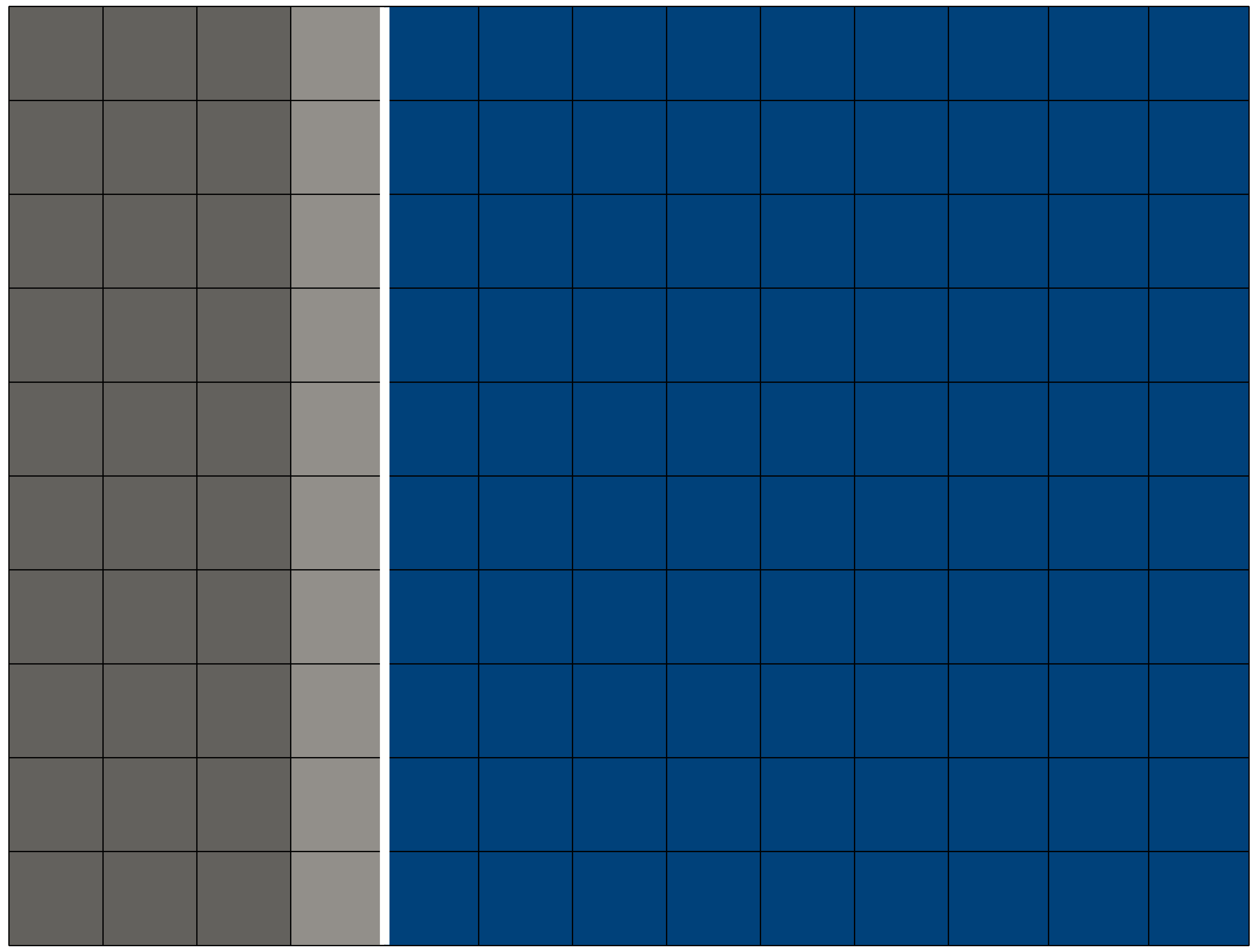
(c) $t=60$ $\mathrm{s}\text{/}$

(d) $t=0$ $\mathrm{s}\text{/}$

(e) $t=15$ $\mathrm{s}\text{/}$

(f) $t=60$ $\mathrm{s}\text{/}$

Figure 7: Dissolution level $d$ at machining times $0$ $\mathrm{s}\text{/}$, $15$ $\mathrm{s}\text{/}$ and $60$ $\mathrm{s}\text{/}$ for a coarse (7(a)-7(c)) and a fine mesh (7(d)-7(f)). The vertical white line indicates the analytical reference solution.

To investigate the influence of the mesh density and the time step size on the simulation, Fig. 8 shows the comparison of the numerically and analytically computed dissolved volume $V_{\mathrm{dis}}$ after $60$ $\mathrm{s}\text{/}$. For the time increment $\Delta t=1~{}$\mathrm{s}\text{/}$$, the coarser meshes ($10\times 10$, $20\times 20$) give results close to the analytical solution $(+\,1.6~{}$\mathrm{\char 37\relax}\text{/}$,\,+\,0.0~{}$\mathrm{\char 37\relax}\text{/}$)$, but slightly differ for smaller time steps, e.g. $\Delta t=0.01~{}$\mathrm{s}\text{/}$$ $(+\,5.4~{}$\mathrm{\char 37\relax}\text{/}$,\,+\,2.6~{}$\mathrm{\char 37\relax}\text{/}$)$. In contrast, the finer meshes ($40\times 40$, $80\times 80$) deviate strongly from the analytical solution for a large time step $\Delta t=1~{}$\mathrm{s}\text{/}$$ $(-\,16.7~{}$\mathrm{\char 37\relax}\text{/}$,\,-\,30.3~{}$\mathrm{\char 37\relax}\text{/}$)$, but converge to the analytical solution for smaller time steps, e.g. $\Delta t=0.01~{}$\mathrm{s}\text{/}$$ $(+\,1.2~{}$\mathrm{\char 37\relax}\text{/}$,\,+\,0.3~{}$\mathrm{\char 37\relax}\text{/}$)$.

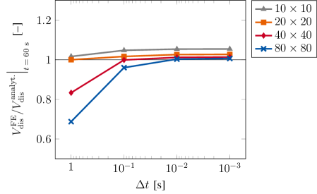
Figure 8: Comparison of dissolved volume from simulation $V_{\mathrm{dis}}^{\mathrm{FE}}$ and analytical solution $V_{\mathrm{dis}}^{\mathrm{analyt.}}$ after a machining time of $60~{}$\mathrm{s}\text{/}$$.

To analyze this result, the cut-off volume $V_{\mathrm{co}}$ is introduced that serves as error indicator. It defines the volume that is theoretically dissolved according to Faraday’s law, but which is neglected numerically when $d_{n+1}>1$ is reset to $d_{n+1}=1$. Moreover, the cut-off volume is accumulated over all time steps $t$, all elements $e$ and all integration points $i$ as follows

$$V_{\mathrm{co}}=\sum_{t=1}^{n_{\mathrm{ts}}}\sum_{e=1}^{n_{\mathrm{el}}}\sum_{i=1}^{n_{\mathrm{gp}}}\left(d_{n+1}-1\right)\,V_{\mathrm{uc}}.$$ (39)

Fig. 9 shows the cut-off volume in relation to the numerically computed dissolved volume after $60$ $\mathrm{s}\text{/}$. The finer meshes, evidently, yield a high relative error $($e.g. $80\times 80,\,\Delta t=1~{}$\mathrm{s}\text{/}$:73.3~{}$\mathrm{\char 37\relax}\text{/}$)$ when using a large time increment. However, this error decreases for all meshes when reducing the time step size.

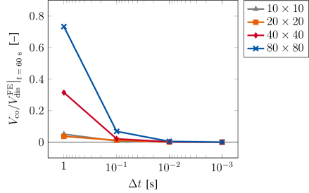
Figure 9: Relative error after a machining time of $60~{}$\mathrm{s}\text{/}$$: Cut-off volume $V_{\mathrm{co}}$ over dissolved volume $V_{\mathrm{dis}}^{\mathrm{FE}}$ for different time increments and meshes.

These findings account for the underestimation of the dissolved volume with fine meshes at large time steps in Fig. 8. Since we update the activation function $\mathcal{A}$, which enables the elements to dissolve, at the end of every time step, a fine mesh using large time steps inevitably causes an underestimation of the dissolved volume. Therefore, the cut-off volume must always be considered and a relative error of e.g. $V_{\mathrm{co}}/V_{\mathrm{dis}}^{\mathrm{FE}}\leq 1~{}$\mathrm{\char 37\relax}\text{/}$$ should be aimed for.

Moreover, we investigate the influence of distorted meshes. To this end, the simulation utilizes three different meshes, where the bottom edge of the workpiece is discretized with $80$ elements and the top edge with $10$, $20$ and $40$ elements, thus, creating a distortion in the transition area (meshes: $10\rightarrow 80$, $20\rightarrow 80$, $40\rightarrow 80$). Fig. 10 shows the dissolution level $d$ for the distorted meshes after $60$ $\mathrm{s}\text{/}$ with $\Delta t=0.01~{}$\mathrm{s}\text{/}$$. The previously defined criterion $V_{\mathrm{co}}/V_{\mathrm{dis}}^{\mathrm{FE}}\leq 1~{}$\mathrm{\char 37\relax}\text{/}$$ holds. The mesh with $10\rightarrow 80$ elements overestimates the dissolved volume by $+\,8.2~{}$\mathrm{\char 37\relax}\text{/}$$. However, the meshes with $20\rightarrow 80$ and $40\rightarrow 80$ elements converge against the correct solution, overestimating the dissolved volume by just $+\,3.6~{}$\mathrm{\char 37\relax}\text{/}$$ and $+\,3.0~{}$\mathrm{\char 37\relax}\text{/}$$. Thus, a dissolving transition zone with extremely different element sizes should be avoided, whereas, moderately distorted meshes yield good results.

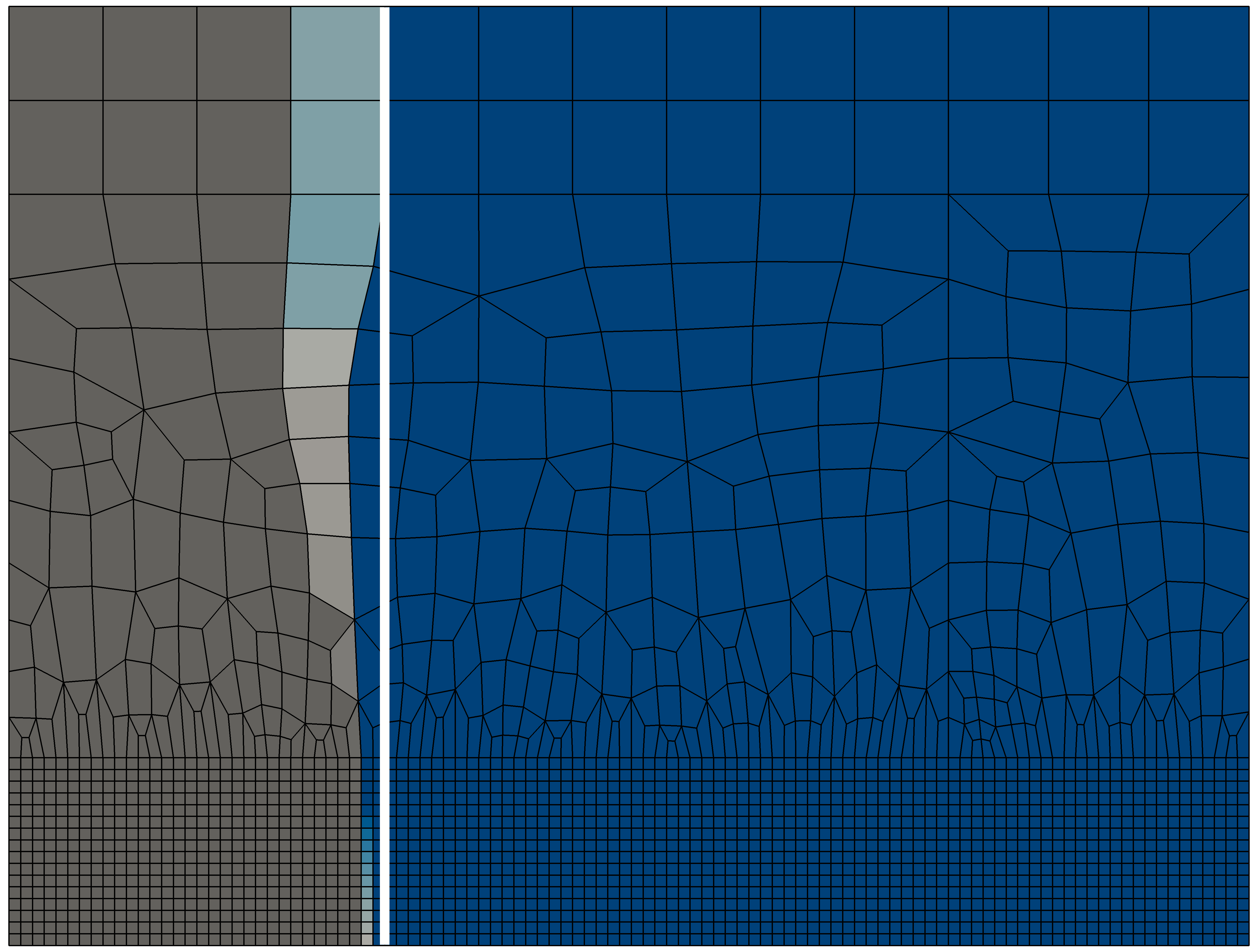
(a) Mesh $10\rightarrow 80$

(b) Mesh $20\rightarrow 80$

(c) Mesh $40\rightarrow 80$

Figure 10: Dissolution level $d$ for distorted meshes at $t=60$ $\mathrm{s}\text{/}$. The vertical white line provides the analytical reference solution.

In summary, this example proves the model’s capability to achieve reasonable results with a coarse mesh at large time steps, and, further, to accurately model material dissolution with fine meshes and time increments.

5.2 Planar specimen - experimental validation

The second example focuses on validating the model’s performance by means of the investigations of Bergs et al. [2019], who electrochemically machine a planar specimen with $l=7\,$\mathrm{mm}\text{/}$$ (Fig. 11(a)). The experiment yields an electrolyte’s inflow temperature of $\widetilde{\theta}_{\mathrm{in}}=298.15\,$\mathrm{K}\text{/}$$. Since the outflow temperature is not determined in this experiment, we assume $\widetilde{\theta}_{\mathrm{out}}=308.15\,$\mathrm{K}\text{/}$$ due to Joule heating in the electrolyte in accordance with Zeis [2015]. We prescribe the inflow temperature at $x=0\,$\mathrm{mm}\text{/}$$ and $y\in[\,-s,\,0.25\,l\,]$ and the outflow temperature at $x=l$ and $y\in[\,-s,\,0.25\,l\,]$ (Fig. 11(b)). For simplicity, we prescribe the temperature at $y\in[\,-s,\,0.25\,l\,]$ during the entire simulation to account for the movement of the electrolyte’s position. Motivated by Zeis [2015] and Harst [2019], we alter the experimental voltage of $\Delta v=15~{}$\mathrm{V}\text{/}$$ in the simulation by a global reduction of $3~{}$\mathrm{V}\text{/}$$ to take a polarization voltage $\Delta v_{\mathrm{pol}}$ at anode and cathode into account. The experimental feed rate is $\dot{x}_{\mathrm{ca}}=1~{}$\mathrm{mm}\text{/}\mathrm{min}$$. For the determination of the working gap width, we compute the electrolyte’s electric conductivity to $k_{\textrm{\tiny E}}^{\textrm{\tiny EL}}=((\widetilde{\theta}_{\mathrm{in}}+\widetilde{\theta}_{\mathrm{out}})/2)=13.7~{}$\mathrm{A}\text{/}\text{(}\mathrm{V}\text{\,}\mathrm{m}\text{)}$$ and, using Eq. (37), obtain $s=0.36~{}$\mathrm{mm}\text{/}$$. We apply the same procedure as in Section 5.1 to model the cathode’s feed and compute $\widetilde{v}_{\mathrm{ca}}(t)$ using Eq. (38). Moreover, the thickness reads $g=0.1~{}$\mathrm{mm}\text{/}$$ and the time increment is $\Delta t=0.01~{}$\mathrm{s}\text{/}$$.

(a) Geometry

(b) BVP

Figure 11: Geometry and boundary value problem of planar specimen (cf. Bergs et al. [2019]).

The simulation utilizes four different meshes starting with a coarse, structured mesh (Fig. 12(a)) followed by a successive mesh refinement in the area of interest (Fig. 12(b)).

(a) Mesh 1 (210 elements)

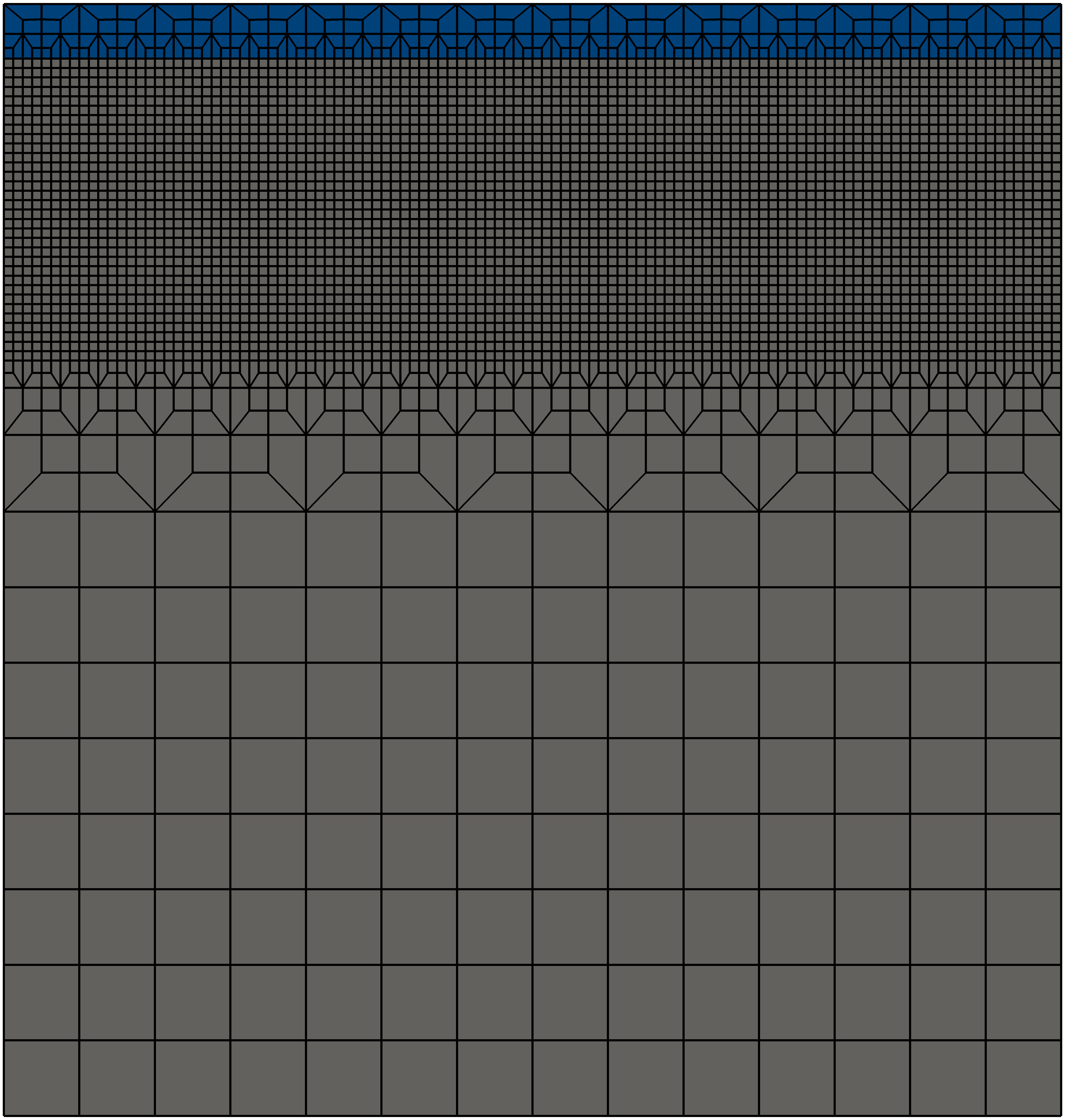
(b) Mesh 4 (4242 elements)

Figure 12: Coarsest and finest mesh for planar specimen with mesh refinement at the workpiece’s surface.

Fig. 13 shows the evolution of the dissolved volume $V_{\mathrm{dis}}$ of Mesh 1 - 4 normalized to $V_{\mathrm{ref}}=120.3~{}${\mathrm{mm}}^{3}\text{/}$$, the dissolved volume of Mesh 4 at $t=100~{}$\mathrm{s}\text{/}$$. Only marginal differences between Mesh 3 and Mesh 4 are visible and, therefore, convergence is assumed. The black boxes indicate the snapshots of the dissolution level $d$ for Mesh 4 in Fig. 15. The error indicator is $V_{\mathrm{co}}/V_{\mathrm{dis}}^{\mathrm{FE}}=0.6~{}$\mathrm{\char 37\relax}\text{/}$$ for the finest mesh.

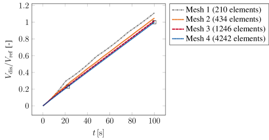
Figure 13: Evolution of dissolved volume $V_{\mathrm{dis}}$ over machining time $t$ of planar specimen for different meshes.

Furthermore, Fig. 14 shows the temperature distribution which results from the assumed boundary conditions. It increases along the working gap and, thereby, models Joule heating in the electrolyte. In experiments, the inflow-temperature usually matches the workpiece’s temperature, which differs in the simulation due to the simplified boundary conditions.

Figure 14: Distribution of temperature $\theta$ for prescribed in- and outflow temperature.

As reported in e.g. Zeis [2015], the electrolyte’s electric conductivity increases with temperature. Therefore, also the electric current density increases along the working gap. Hence, the simulation yields an increased removal of material and widening of the working gap. For a small machining depth, the anode’s surface is slightly inclined (Fig. 15(a)), but for a large machining depth, a pronounced inclination and working gap widening occurs (Fig. 15(b)). These results show satisfactory agreement with the investigations of Bergs et al. [2019]. However, Bergs et al. [2019] observe a slightly higher inclination of the machined surface than $\beta_{2}\approx 1.04$\mathrm{\SIUnitSymbolDegree}\text{/}$$ for a large machining depth. Due to the lack of detailed information about the temperature distribution in the machining gap, the numerical results may vary.

(a) Small machining depth

(b) Large machining depth

Figure 15: Dissolution level $d$ of planar specimen at different machining depths. The inclination $\beta$ of the machined surface increases with the machining depth $\left(\beta_{2}\approx 1.04$\mathrm{\SIUnitSymbolDegree}\text{/}$>\beta_{1}\approx 0.38$\mathrm{\SIUnitSymbolDegree}\text{/}$\right)$.

5.3 Curved specimen with elevation - experimental validation

This example investigates a specimen with a non-planar surface, which is curved and possesses an elevation. Thus, inhomogeneous material removal at the beginning of the ECM-process can be examined. Bergs et al. [2019] also study this geometry and the parameters read $x_{1}=0.5~{}$\mathrm{mm}\text{/}$$, $x_{2}=3~{}$\mathrm{mm}\text{/}$$, $y_{1}=0.25~{}$\mathrm{mm}\text{/}$$, $y_{2}=0.5~{}$\mathrm{mm}\text{/}$$ and $l=7~{}$\mathrm{mm}\text{/}$$ (Fig. 16(a)). A parabola defines the curvature with the vertex of the parabola at position $(1.5~{}$\mathrm{mm}\text{/}$\,|\,0.3~{}$\mathrm{mm}\text{/}$)$. The gap width $s=0.36~{}$\mathrm{mm}\text{/}$$ is adopted from Section 5.2. The remaining process parameters and boundary conditions are analogous to Section 5.2 (Fig. 16(b)).

(a) Geometry

(b) BVP

Figure 16: Geometry and boundary value problem of curved specimen with elevation (cf. Bergs et al. [2019]).

Figure 17: Mesh (6448 elements) of curved specimen with elevation.

Further, Fig. 17 shows the mesh which is employed in the simulation. The mesh possesses strong mesh refinement at the upper part of the workpiece where material dissolution occurs. The simulation yields $V_{\mathrm{co}}/V_{\mathrm{dis}}^{\mathrm{FE}}=0.7~{}$\mathrm{\char 37\relax}\text{/}$$ at the end of the simulation and, therefore, mesh density and time step size fit.

Fig. 18 shows the dissolution level $d$ after $10~{}$\mathrm{s}\text{/}$$, $25~{}$\mathrm{s}\text{/}$$, $50~{}$\mathrm{s}\text{/}$$ and $125~{}$\mathrm{s}\text{/}$$ machining time. In the initial stages of the process, increased material removal occurs at the tip of the specimen (Figs. 18(a) and 18(b)). At this position, the electric field lines increase in density and, thus, lead to a higher electric current density and removal of the elevation. As the process continues, the specimen’s curvature starts to smooth out (Fig. 18(c)) until an approximately planar surface evolves (Fig. 18(d)). To remove the curvature, we require a machining depth larger than two and a half times of the initial imperfection of the specimen. These results conform with the findings of Bergs et al. [2019].

(a) $t=10$ $\mathrm{s}\text{/}$

(b) $t=25$ $\mathrm{s}\text{/}$

(c) $t=50$ $\mathrm{s}\text{/}$

(d) $t=125$ $\mathrm{s}\text{/}$

Figure 18: Dissolution level $d$ at different machining times of curved specimen with elevation. The material removal focuses on the elevation before a level surface emerges.

The example validates the model’s capability to exactly simulate material dissolution in the electrochemical machining process.

5.4 Pulsed electrochemical machining

Finally, we apply the model to predict the evolution of the surface roughness in a electrochemical machining application with electrical pulses (PECM). Fig. 19(a) shows the exemplary setup of the PECM-process. The working gap width measures $s=51.875~{}$\mathrm{\SIUnitSymbolMicro m}\text{/}$$ and the width of the analyzed surface $w=20~{}$\mathrm{\SIUnitSymbolMicro m}\text{/}$$. We consider an idealized roughness profile with an initial peak value of $p=6.25~{}$\mathrm{\SIUnitSymbolMicro m}\text{/}$$. The remaining parameters read $h=21.875~{}$\mathrm{\SIUnitSymbolMicro m}\text{/}$$, $r=0.625~{}$\mathrm{\SIUnitSymbolMicro m}\text{/}$$, $x_{1}=2.5~{}$\mathrm{\SIUnitSymbolMicro m}\text{/}$$, $y_{1}=5~{}$\mathrm{\SIUnitSymbolMicro m}\text{/}$$ and thickness $g=1~{}$\mathrm{\SIUnitSymbolMicro m}\text{/}$$. Due to the short flow length, we neglect a temperature gradient and set the temperature to $\widetilde{\theta}=298.15~{}$\mathrm{K}\text{/}$$. The time increment is $\Delta t=0.01~{}$\mathrm{ms}\text{/}$$. We neglect the polarization voltage, define the electric potential at the cathode to $\widetilde{v}_{\mathrm{ca}}=0~{}$\mathrm{V}\text{/}$$ and apply a sawtooth cyclic loading pattern at the anode with $\widetilde{v}_{\mathrm{max}}=20~{}$\mathrm{V}\text{/}$$ and $t_{\mathrm{pulse}}=4~{}$\mathrm{ms}\text{/}$$ for the electric potential (Fig. 19(b)). This example assumes stationary electrode’s positions and, thus, precise boundary conditions for the electric potential.

(a) Geometry

(b) BVP

Figure 19: Geometry and boundary value problem of exemplary PECM setup.

Furthermore, Fig. 20 shows the mesh which exhibits strong refinement at the workpiece’s surface. The simulation yields $V_{\mathrm{co}}/V_{\mathrm{dis}}^{\mathrm{FE}}=1.5~{}$\mathrm{\char 37\relax}\text{/}$$ which is deemed reasonable, since this is an example of principle.

Figure 20: Mesh (11264 elements) for PECM with refinement at the anode’s surface.

Next, we introduce two measures for the surface roughness according to DIN EN ISO 25178-2 [2012]: First, the maximum height $Rz$ that defines the distance from the maximum peak height to the minimum pit depth

$$Rz=\|y_{\mathrm{max}}-y_{\mathrm{min}}\|.$$ (40)

Second, the arithmetical mean height $Ra$ which is computed according to

$$Ra=\frac{1}{L_{x}}\,\int_{0}^{L_{x}}\|y(x)-\bar{y}\|\,\mathrm{d}x,\hskip 22.76219pt\bar{y}=\frac{1}{L_{x}}\,\int_{0}^{L_{x}}y(x)\,\mathrm{d}x.$$ (41)

The center of each element, where the activation function is active, serves to define the surface’s roughness profile. With these discrete values, we compute the roughness values $Rz$ and $Ra$ at every time step.

“A Process Signature is based on the correlation between the internal material loads in manufacturing processes (e.g., stress, strain, temperature) and the resulting material modifications“ (Brinksmeier et al. [2018]). Here, the material load $Q/A$ is the accumulated electric charge, which passes in vertical direction, divided by the specimen’s cross section. The material modification is the evolution of the surface roughness. Other authors, e.g. Harst [2019] employ the electric field strength $\bm{E}$ as material load in ECM. Fig. 21 shows the corresponding process signature of both roughness measures $Rz$ and $Ra$ for an exemplary initial surface roughness. Starting with the initial values $Rz=6.23~{}$\mathrm{\SIUnitSymbolMicro m}\text{/}$$ and $Ra=1.70~{}$\mathrm{\SIUnitSymbolMicro m}\text{/}$$, both roughness measures decrease hyperbolically to zero. The black boxes indicate the snapshots given in Fig. 22.

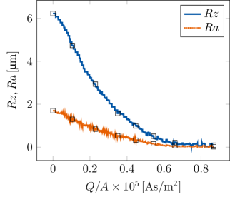
Figure 21: Process signature of surface roughness.

Fig. 22 shows the surface profile for different machining times. First, the material dissolves at the tip of the spikes (Figs. 22(b) - 22(c)). Then, the bodies of the spikes dissolve (Figs. 22(d) - 22(g)) until a level surface evolves (Fig. 22(h)).

(a) $0~{}$\mathrm{ms}\text{/}$$

(b) $5~{}$\mathrm{ms}\text{/}$$

(c) $10~{}$\mathrm{ms}\text{/}$$

(d) $15~{}$\mathrm{ms}\text{/}$$

(e) $20~{}$\mathrm{ms}\text{/}$$

(f) $25~{}$\mathrm{ms}\text{/}$$

(g) $30~{}$\mathrm{ms}\text{/}$$

(h) $40~{}$\mathrm{ms}\text{/}$$

Figure 22: Dissolution level $d$ and surface profile for different machining times in PECM.

This example proves the applicability of the model to compute process signatures that focus on the surface roughness in PECM and, additionally, to simulate a process with multiple electrical loads.

6 Conclusion

This paper presented an innovative method to efficiently model anodic dissolution in ECM, which circumvents the need for computationally expensive remeshing. At first, we define the dissolution level and the corresponding effective material parameters at integration point level. Next, we discuss the coupled problem of thermoelectricity and the numerical implementation in detail. Thereafter, numerical investigations validate the model’s performance and accuracy by analytical and experimental reference solutions. In particular, the influence of the finite element mesh density and the time step size is investigated. The model shows – even in the case of rather coarse meshes – a highly satisfactory predictability. Moreover, the comparison with experiments confirms the realistic results obtained by means of numerical simulations. Finally, the model enables the computation of a process signature of the surface roughness with multiple electrical loads. The process signature’s corresponding material modification is the evolution of the maximum and the arithmetical mean height. Additionally, the specific accumulated electric charge defines the corresponding material load. Future work includes the modeling of multiphase materials with different polarization voltages, the exact description of the moving boundary value problem and the incorporation of fluid mechanical effects.

Acknowledgements

Funding granted by the subprojects M05 - “Numerically efficient multi scale material models for processes under thermal and chemical impact” and F03 - “Processes with chemical impact” of the transregional Collaborative Research Center 136 “Process Signatures” with the project number 223500200 is gratefully acknowledged.

Appendix A Appendix

A.1 Linearization

The linearization of $g_{v}$ and $g_{\theta}$ (Eqs. (19) and (20)) about a known state $\left(\bar{v}_{n+1},\bar{\theta}_{n+1}\right)$ reads:

$$L_{g_{v}} =g_{v}\left(\bar{v}_{n+1},\,\bar{\theta}_{n+1},\,\delta v\right)$$

$$\hskip 56.9055pt+\Delta_{v}g_{v}\left(\bar{v}_{n+1},\,\bar{\theta}_{n+1},\,\delta v,\,\Delta v_{n+1}\right)$$

$$\hskip 113.81102pt+\Delta_{\theta}g_{v}\left(\bar{v}_{n+1},\,\bar{\theta}_{n+1},\,\delta v,\,\Delta\theta_{n+1}\right)\stackrel{{\scriptstyle!}}{{=}}0\qquad\forall\,\delta v$$ (42)

$$L_{g_{\theta}} =g_{\theta}\left(\bar{v}_{n+1},\,\bar{\theta}_{n+1},\,\delta\theta\right)$$

$$\hskip 56.9055pt+\Delta_{v}g_{\theta}\left(\bar{v}_{n+1},\,\bar{\theta}_{n+1},\,\delta\theta,\,\Delta v_{n+1}\right)$$

$$\hskip 113.81102pt+\Delta_{\theta}g_{\theta}\left(\bar{v}_{n+1},\,\bar{\theta}_{n+1},\,\delta\theta,\,\Delta\theta_{n+1}\right)\stackrel{{\scriptstyle!}}{{=}}0\qquad\forall\,\delta\theta$$ (43)

Furthermore, the Gâteaux-derivatives are defined as follows:

$$\Delta_{v}g_{v}\left(\bar{v}_{n+1},\,\bar{\theta}_{n+1},\,\delta v,\,\Delta v_{n+1}\right) \mathrel{\leavevmode\resizebox{0.0pt}{0.0pt}{ $\!\!\leavevmode\resizebox{1.2pt}{0.8pt}{\raisebox{0.99025pt}{$\mathop{:}$}}\!\!=\!\!$ }}\frac{{\rm d}}{{\rm d}\alpha}\Big{[}g_{v}\left(\bar{v}_{n+1}+\alpha\,\Delta v_{n+1},\,\bar{\theta}_{n+1},\,\delta v\right)\Big{]}_{\alpha=0}$$ (44)

$$\Delta_{\theta}g_{v}\left(\bar{v}_{n+1},\,\bar{\theta}_{n+1},\,\delta v,\,\Delta\theta_{n+1}\right) \mathrel{\leavevmode\resizebox{0.0pt}{0.0pt}{ $\!\!\leavevmode\resizebox{1.2pt}{0.8pt}{\raisebox{0.99025pt}{$\mathop{:}$}}\!\!=\!\!$ }}\frac{{\rm d}}{{\rm d}\alpha}\Big{[}g_{v}\left(\bar{v}_{n+1},\,\bar{\theta}_{n+1}+\alpha\,\Delta\theta_{n+1},\,\delta v\right)\Big{]}_{\alpha=0}$$ (45)

$$\Delta_{v}g_{\theta}\left(\bar{v}_{n+1},\,\bar{\theta}_{n+1},\,\delta\theta,\,\Delta v_{n+1}\right) \mathrel{\leavevmode\resizebox{0.0pt}{0.0pt}{ $\!\!\leavevmode\resizebox{1.2pt}{0.8pt}{\raisebox{0.99025pt}{$\mathop{:}$}}\!\!=\!\!$ }}\frac{{\rm d}}{{\rm d}\alpha}\Big{[}g_{\theta}\left(\bar{v}_{n+1}+\alpha\,\Delta v_{n+1},\,\bar{\theta}_{n+1},\,\delta\theta\right)\Big{]}_{\alpha=0}$$ (46)

$$\Delta_{\theta}g_{\theta}\left(\bar{v}_{n+1},\,\bar{\theta}_{n+1},\,\delta\theta,\,\Delta\theta_{n+1}\right) \mathrel{\leavevmode\resizebox{0.0pt}{0.0pt}{ $\!\!\leavevmode\resizebox{1.2pt}{0.8pt}{\raisebox{0.99025pt}{$\mathop{:}$}}\!\!=\!\!$ }}\frac{{\rm d}}{{\rm d}\alpha}\Big{[}g_{\theta}\left(\bar{v}_{n+1},\,\bar{\theta}_{n+1}+\alpha\,\Delta\theta_{n+1},\,\delta\theta\right)\Big{]}_{\alpha=0}$$ (47)

In detail, the linearization of $g_{v}$ with respect to $v_{n+1}$ reads:

$$\Delta_{v}g_{v} =\frac{{\rm d}}{{\rm d}\alpha}\bigg{[}-\int_{\Omega}\bm{j}_{\textrm{\tiny L}}\left(\bm{E}\left(\alpha\right)\right)\cdot{\rm grad}\left(\delta v\right)\mathrm{d}V$$

$$\hskip 71.13188pt-2\int_{\Omega}\bm{j}_{\textrm{\tiny V}}\left(\dot{\bm{E}}\left(\alpha\right)\right)\cdot{\rm grad}\left(\delta v\right)\mathrm{d}V\bigg{]}_{\alpha=0}$$

$$=\hskip 15.649pt\bigg{[}-\int_{\Omega}\left(\displaystyle\frac{\partial\bm{j}_{\textrm{\tiny L}}}{\partial\bm{E}}\cdot\displaystyle\frac{\partial\bm{E}}{\partial\alpha}\right)\cdot{\rm grad}\left(\delta v\right)\mathrm{d}V$$

$$\hskip 71.13188pt-2\int_{\Omega}\left(\displaystyle\frac{\partial\bm{j}_{\textrm{\tiny V}}}{\partial\dot{\bm{E}}}\cdot\displaystyle\frac{\partial\dot{\bm{E}}}{\partial\alpha}\right)\cdot{\rm grad}\left(\delta v\right)\mathrm{d}V\bigg{]}_{\alpha=0}$$

$$=\hskip 28.45274pt-\int_{\Omega}\left(\displaystyle\frac{\partial\bm{j}_{\textrm{\tiny L}}}{\partial\bm{E}}\cdot\left(-{\rm grad}\left(\Delta v_{n+1}\right)\right)\right)\cdot{\rm grad}\left(\delta v\right)\mathrm{d}V$$

$$\hskip 71.13188pt-2\int_{\Omega}\left(\displaystyle\frac{\partial\bm{j}_{\textrm{\tiny V}}}{\partial\dot{\bm{E}}}\cdot\frac{1}{\Delta t}\left(-{\rm grad}\left(\Delta v_{n+1}\right)\right)\right)\cdot{\rm grad}\left(\delta v\right)\mathrm{d}V$$ (48)

In detail, the linearization of $g_{v}$ with respect to $\theta_{n+1}$ reads:

$$\Delta_{\theta}g_{v} =\frac{{\rm d}}{{\rm d}\alpha}\bigg{[}-\int_{\Omega}\bm{j}_{\textrm{\tiny S}}\left({\rm grad}\left(\theta_{n+1}\left(\alpha\right)\right)\right)\cdot{\rm grad}\left(\delta v\right)\mathrm{d}V\bigg{]}_{\alpha=0}$$

$$=\hskip 16.5026pt\bigg{[}-\int_{\Omega}\left(\displaystyle\frac{\partial\bm{j}_{\textrm{\tiny S}}}{\partial{\rm grad}\left(\theta_{n+1}\right)}\cdot\displaystyle\frac{\partial{\rm grad}\left(\theta_{n+1}\right)}{\partial\alpha}\right)\cdot{\rm grad}\left(\delta v\right)\mathrm{d}V\bigg{]}_{\alpha=0}$$

$$=\hskip 25.32292pt-\int_{\Omega}\left(\displaystyle\frac{\partial\bm{j}_{\textrm{\tiny S}}}{\partial{\rm grad}\left(\theta_{n+1}\right)}\cdot{\rm grad}\left(\Delta\theta_{n+1}\right)\right)\cdot{\rm grad}\left(\delta v\right)\mathrm{d}V$$ (49)

In detail, the linearization of $g_{\theta}$ with respect to $v_{n+1}$ reads:

$$\Delta_{v}g_{\theta} =\frac{{\rm d}}{{\rm d}\alpha}\bigg{[}-\int_{\Omega}\bar{\Pi}\left(d_{n},\theta_{n}\right)\bm{j}_{\textrm{\tiny L}}\left(\bm{E}\left(\alpha\right)\right)\cdot{\rm grad}\left(\delta\theta\right)\mathrm{d}V$$

$$\hskip 71.13188pt-\int_{\Omega}\bar{\Pi}\left(d_{n},\theta_{n}\right)\bm{j}_{\textrm{\tiny V}}\left(\dot{\bm{E}}\left(\alpha\right)\right)\cdot{\rm grad}\left(\delta\theta\right)\mathrm{d}V$$

$$\hskip 113.81102pt-\int_{\Omega}\bm{j}_{\textrm{\tiny L}}\left(\bm{E}\left(\alpha\right)\right)\cdot\bm{E}\left(\alpha\right)\delta\theta\,\mathrm{d}V$$

$$\hskip 156.49014pt-\int_{\Omega}\bm{j}_{\textrm{\tiny V}}\left(\dot{\bm{E}}\left(\alpha\right)\right)\cdot\bm{E}\left(\alpha\right)\delta\theta\,\mathrm{d}V$$

$$\hskip 199.16928pt-\int_{\Omega}\bm{j}_{\textrm{\tiny S}}\cdot\bm{E}\left(\alpha\right)\delta\theta\,\mathrm{d}V\bigg{]}_{\alpha=0}$$

$$=\hskip 15.649pt\bigg{[}-\int_{\Omega}\left(\bar{\Pi}\left(d_{n},\theta_{n}\right)\displaystyle\frac{\partial\bm{j}_{\textrm{\tiny L}}}{\partial\bm{E}}\cdot\displaystyle\frac{\partial\bm{E}}{\partial\alpha}\right)\cdot{\rm grad}\left(\delta\theta\right)\mathrm{d}V$$

$$\hskip 71.13188pt-\int_{\Omega}\left(\bar{\Pi}\left(d_{n},\theta_{n}\right)\displaystyle\frac{\partial\bm{j}_{\textrm{\tiny V}}}{\partial\dot{\bm{E}}}\cdot\displaystyle\frac{\partial\dot{\bm{E}}}{\partial\alpha}\right)\cdot{\rm grad}\left(\delta\theta\right)\mathrm{d}V$$

$$\hskip 113.81102pt-\int_{\Omega}\left(\left(\displaystyle\frac{\partial\bm{j}_{\textrm{\tiny L}}}{\partial\bm{E}}\cdot\displaystyle\frac{\partial\bm{E}}{\partial\alpha}\right)\cdot\bm{E}\left(\alpha\right)+\bm{j}_{\textrm{\tiny L}}\left(\bm{E}\left(\alpha\right)\right)\cdot\displaystyle\frac{\partial\bm{E}}{\partial\alpha}\right)\delta\theta\,\mathrm{d}V$$

$$\hskip 156.49014pt-\int_{\Omega}\left(\left(\displaystyle\frac{\partial\bm{j}_{\textrm{\tiny V}}}{\partial\dot{\bm{E}}}\cdot\displaystyle\frac{\partial\dot{\bm{E}}}{\partial\alpha}\right)\cdot\bm{E}\left(\alpha\right)+\bm{j}_{\textrm{\tiny V}}\left(\dot{\bm{E}}\left(\alpha\right)\right)\cdot\displaystyle\frac{\partial\bm{E}}{\partial\alpha}\right)\delta\theta\,\mathrm{d}V$$

$$\hskip 199.16928pt-\int_{\Omega}\left(\bm{j}_{\textrm{\tiny S}}\cdot\displaystyle\frac{\partial\bm{E}}{\partial\alpha}\right)\delta\theta\,\mathrm{d}V\bigg{]}_{\alpha=0}$$

$$=\hskip 28.45274pt-\int_{\Omega}\left(\bar{\Pi}\left(d_{n},\theta_{n}\right)\displaystyle\frac{\partial\bm{j}_{\textrm{\tiny L}}}{\partial\bm{E}}\cdot\left(-{\rm grad}\left(\Delta v_{n+1}\right)\right)\right)\cdot{\rm grad}\left(\delta\theta\right)\mathrm{d}V$$

$$\hskip 71.13188pt-\int_{\Omega}\left(\bar{\Pi}\left(d_{n},\theta_{n}\right)\displaystyle\frac{\partial\bm{j}_{\textrm{\tiny V}}}{\partial\dot{\bm{E}}}\cdot\frac{1}{\Delta t}\left(-{\rm grad}\left(\Delta v_{n+1}\right)\right)\right)\cdot{\rm grad}\left(\delta\theta\right)\mathrm{d}V$$

$$\hskip 113.81102pt-\int_{\Omega}2\,\bm{j}_{\textrm{\tiny L}}\cdot\left(-{\rm grad}\left(\Delta v_{n+1}\right)\right)\delta\theta\,\mathrm{d}V$$

$$\hskip 156.49014pt-\int_{\Omega}\left(\displaystyle\frac{\partial\bm{j}_{\textrm{\tiny V}}}{\partial\dot{\bm{E}}}\cdot\frac{1}{\Delta t}\,\bm{E}+\bm{j}_{\textrm{\tiny V}}\right)\cdot\left(-{\rm grad}\left(\Delta v_{n+1}\right)\right)\delta\theta\,\mathrm{d}V$$

$$\hskip 199.16928pt-\int_{\Omega}\,\bm{j}_{\textrm{\tiny S}}\cdot\left(-{\rm grad}\left(\Delta v_{n+1}\right)\right)\delta\theta\,\mathrm{d}V$$ (50)

In detail, the linearization of $g_{\theta}$ with respect to $\theta_{n+1}$ reads:

$$\Delta_{\theta}g_{\theta} =\frac{{\rm d}}{{\rm d}\alpha}\bigg{[}-\int_{\Omega}\bar{\Pi}\left(d_{n},\theta_{n}\right)\bm{j}_{\textrm{\tiny S}}\left({\rm grad}\left(\theta_{n+1}\left(\alpha\right)\right)\right)\cdot{\rm grad}\left(\delta\theta\right)\mathrm{d}V$$

$$\hskip 71.13188pt-\int_{\Omega}\bm{q}_{\textrm{\tiny F}}\left({\rm grad}\left(\theta_{n+1}\left(\alpha\right)\right)\right)\cdot{\rm grad}\left(\delta\theta\right)\mathrm{d}V$$

$$\hskip 113.81102pt+\int_{\Omega}\bar{\rho}_{\textrm{\tiny V}}\bar{c}_{\theta}\,\dot{\theta}_{n+1}\left(\alpha\right)\,\delta\theta\,\mathrm{d}V$$

$$\hskip 156.49014pt-\int_{\Omega}\bm{j}_{\textrm{\tiny S}}\left({\rm grad}\left(\theta_{n+1}\left(\alpha\right)\right)\right)\cdot\bm{E}\,\delta\theta\,\mathrm{d}V\bigg{]}_{\alpha=0}$$

$$=\hskip 15.649pt\bigg{[}-\int_{\Omega}\left(\bar{\Pi}\left(d_{n},\theta_{n}\right)\displaystyle\frac{\partial\bm{j}_{\textrm{\tiny S}}}{\partial{\rm grad}\left(\theta_{n+1}\right)}\cdot\displaystyle\frac{\partial{\rm grad}\left(\theta_{n+1}\right)}{\partial\alpha}\right)\cdot{\rm grad}\left(\delta\theta\right)\mathrm{d}V$$

$$\hskip 71.13188pt-\int_{\Omega}\left(\displaystyle\frac{\partial\bm{q}_{\textrm{\tiny F}}}{\partial{\rm grad}\left(\theta_{n+1}\right)}\cdot\displaystyle\frac{\partial{\rm grad}\left(\theta_{n+1}\right)}{\partial\alpha}\right)\cdot{\rm grad}\left(\delta\theta\right)\mathrm{d}V$$

$$\hskip 113.81102pt+\int_{\Omega}\bar{\rho}_{\textrm{\tiny V}}\bar{c}_{\theta}\,\frac{1}{\Delta t}\,\Delta\theta_{n+1}\,\delta\theta\,\mathrm{d}V$$

$$\hskip 156.49014pt-\int_{\Omega}\left(\displaystyle\frac{\partial\bm{j}_{\textrm{\tiny S}}}{\partial{\rm grad}\left(\theta_{n+1}\right)}\cdot\displaystyle\frac{\partial{\rm grad}\left(\theta_{n+1}\right)}{\partial\alpha}\right)\cdot\bm{E}\,\delta\theta\,\mathrm{d}V\bigg{]}_{\alpha=0}$$

$$=\hskip 28.45274pt-\int_{\Omega}\left(\bar{\Pi}\left(d_{n},\theta_{n}\right)\displaystyle\frac{\partial\bm{j}_{\textrm{\tiny S}}}{\partial{\rm grad}\left(\theta_{n+1}\right)}\cdot{\rm grad}\left(\Delta\theta_{n+1}\right)\right)\cdot{\rm grad}\left(\delta\theta\right)\mathrm{d}V$$

$$\hskip 71.13188pt-\int_{\Omega}\left(\displaystyle\frac{\partial\bm{q}_{\textrm{\tiny F}}}{\partial{\rm grad}\left(\theta_{n+1}\right)}\cdot{\rm grad}\left(\Delta\theta_{n+1}\right)\right)\cdot{\rm grad}\left(\delta\theta\right)\mathrm{d}V$$

$$\hskip 113.81102pt+\int_{\Omega}\bar{\rho}_{\textrm{\tiny V}}\bar{c}_{\theta}\,\frac{1}{\Delta t}\,\Delta\theta_{n+1}\,\delta\theta\,\mathrm{d}V$$

$$\hskip 156.49014pt-\int_{\Omega}\left(\displaystyle\frac{\partial\bm{j}_{\textrm{\tiny S}}}{\partial{\rm grad}\left(\theta_{n+1}\right)}\cdot{\rm grad}\left(\Delta\theta_{n+1}\right)\right)\cdot\bm{E}\,\delta\theta\,\mathrm{d}V$$ (51)

In addition, the corresponding tangents in Eqs. (48) - (51) read:

$$\displaystyle\frac{\partial\bm{j}_{\textrm{\tiny L}}}{\partial\bm{E}} =\bar{k}_{\textrm{\tiny E}}\left(d_{n},\theta_{n}\right)\mathbf{I}$$ (52)

$$\displaystyle\frac{\partial\bm{j}_{\textrm{\tiny V}}}{\partial\dot{\bm{E}}} =\epsilon_{\mathrm{0}}\bar{\epsilon}_{\mathrm{r}}\,\mathbf{I}$$ (53)

$$\displaystyle\frac{\partial\bm{j}_{\textrm{\tiny S}}}{\partial{\rm grad}\left(\theta_{n+1}\right)} =-\bar{k}_{\textrm{\tiny E}}\left(d_{n},\theta_{n}\right)\,\bar{\alpha}\left(d_{n},\theta_{n}\right)\mathbf{I}$$ (54)

$$\displaystyle\frac{\partial\bm{q}_{\textrm{\tiny F}}}{\partial{\rm grad}\left(\theta_{n+1}\right)} =-\bar{k}_{\theta}\left(d_{n},\theta_{n}\right)\mathbf{I}$$ (55)

A.2 Element vectors and matrices

$$\mathbf{k}_{vv}^{e} =\hphantom{-}\int_{\Omega^{e}}\mathbf{B}_{v}^{e\mathrm{T}}\,\left(\displaystyle\frac{\partial\bm{j}_{\textrm{\tiny L}}}{\partial\bm{E}}\right)^{e}\,\mathbf{B}_{v}^{e}\,\mathrm{d}V^{e}$$ (56)

$$\mathbf{k}_{v\theta}^{e} =-\int_{\Omega^{e}}\mathbf{B}_{v}^{e\mathrm{T}}\,\left(\displaystyle\frac{\partial\bm{j}_{\textrm{\tiny S}}}{\partial{\rm grad}\left(\theta_{n+1}\right)}\right)^{e}\,\mathbf{B}_{\theta}^{e}\,\mathrm{d}V^{e}$$ (57)

$$\mathbf{k}_{\theta v}^{e} =\hphantom{-}\int_{\Omega^{e}}\bm{N}_{\theta}^{e\mathrm{T}}\,\left(2\,\bm{j}_{\textrm{\tiny L}}^{e}+\bm{j}_{\textrm{\tiny S}}^{e}\right)^{\mathrm{T}}\,\mathbf{B}_{v}^{e}+\mathbf{B}_{\theta}^{e\mathrm{T}}\,\bar{\Pi}^{e}\left(\displaystyle\frac{\partial\bm{j}_{\textrm{\tiny L}}}{\partial\bm{E}}\right)^{e}\,\mathbf{B}_{v}^{e}\,\mathrm{d}V^{e}$$ (58)

$$\mathbf{k}_{\theta\theta}^{e} =-\int_{\Omega^{e}}\bm{N}_{\theta}^{e\mathrm{T}}\,\bm{E}^{e\mathrm{T}}\,\left(\displaystyle\frac{\partial\bm{j}_{\textrm{\tiny S}}}{\partial{\rm grad}\left(\theta_{n+1}\right)}\right)^{e}\,\mathbf{B}_{\theta}^{e}\,\mathrm{d}V^{e}$$

$$\hskip 12.80373pt-\int_{\Omega^{e}}\mathbf{B}_{\theta}^{e\mathrm{T}}\,\left(\bar{\Pi}^{e}\left(\displaystyle\frac{\partial\bm{j}_{\textrm{\tiny S}}}{\partial{\rm grad}\left(\theta_{n+1}\right)}\right)^{e}+\left(\displaystyle\frac{\partial\bm{q}_{\textrm{\tiny F}}}{\partial{\rm grad}\left(\theta_{n+1}\right)}\right)^{e}\,\right)\,\mathbf{B}_{\theta}^{e}\,\mathrm{d}V^{e}$$ (59)

$$\mathbf{c}_{vv}^{e} =\hskip 4.2679pt2\int_{\Omega^{e}}\mathbf{B}_{v}^{e\mathrm{T}}\,\frac{1}{\Delta t}\left(\displaystyle\frac{\partial\bm{j}_{\textrm{\tiny V}}}{\partial\dot{\bm{E}}}\right)^{e}\,\mathbf{B}_{v}^{e}\,\mathrm{d}V^{e}$$ (60)

$$\mathbf{c}_{\theta v}^{e} =\hphantom{-}\int_{\Omega^{e}}\bm{N}_{\theta}^{e\mathrm{T}}\,\left(\frac{1}{\Delta t}\left(\displaystyle\frac{\partial\bm{j}_{\textrm{\tiny V}}}{\partial\dot{\bm{E}}}\right)^{e}\bm{E}^{e}+\,\bm{j}_{\textrm{\tiny V}}^{e}\right)^{\mathrm{T}}\,\mathbf{B}_{v}^{e}+\mathbf{B}_{\theta}^{e\mathrm{T}}\,\frac{1}{\Delta t}\,\bar{\Pi}^{e}\left(\displaystyle\frac{\partial\bm{j}_{\textrm{\tiny V}}}{\partial\dot{\bm{E}}}\right)^{e}\,\mathbf{B}_{v}^{e}\,\mathrm{d}V^{e}$$ (61)

$$\mathbf{c}_{\theta\theta}^{e} =\hphantom{-}\int_{\Omega^{e}}\bm{N}_{\theta}^{e\mathrm{T}}\,\frac{1}{\Delta t}\,\bar{\rho}_{\textrm{\tiny V}}^{\,e}\bar{c}_{\theta}^{\,e}\,\bm{N}_{\theta}^{e}\,\mathrm{d}V^{e}$$ (62)

$$\bm{r}_{v}^{e} =-\int_{\Omega^{e}}\mathbf{B}_{v}^{e\mathrm{T}}\,\left(\bm{j}^{e}+\bm{j}_{\textrm{\tiny V}}^{e}\right)\mathrm{d}V^{e}$$ (63)

$$\bm{r}_{\theta}^{e} =\hphantom{-}\int_{\Omega^{e}}\bm{N}_{\theta}^{e\mathrm{T}}\left(\bar{\rho}_{\textrm{\tiny V}}^{\,e}\bar{c}_{\theta}^{\,e}\dot{\theta}^{e}-\bm{j}^{e\mathrm{T}}\,\bm{E}^{e}-q^{\ast}\right)\mathrm{d}V^{e}-\int_{\Omega^{e}}\mathbf{B}_{v}^{e\mathrm{T}}\,\bm{q}^{e}\,\mathrm{d}V^{e}$$ (64)

References

- [1]
- Antonova and Looman [2005] Antonova, E. E. and Looman, D. C. [2005], ‘Finite elements for thermoelectric device analysis in ansys’, IEEE. ICT 2005. 24th International Conference on Thermoelectrics 2005, 215–218.
- Bergs and Harst [2020] Bergs, T. and Harst, S. [2020], ‘Development of a process signature for electrochemical machining’, CIRP Annals 69, 153 – 156.
- Bergs et al. [2019] Bergs, T., Rommes, B., Harst, S., Herrig, T. and Klink, A. [2019], ‘Influence of initial geometric deviations on the shaping accuracy during electrochemical machining’, Proceedings INSECT pp. 61–66.
- Brepols et al. [2017] Brepols, T., Wulfinghoff, S. and Reese, S. [2017], ‘Gradient-extended two-surface damage-plasticity: Micromorphic formulation and numerical aspects’, International Journal of Plasticity 97, 64 – 106.
- Brepols et al. [2020] Brepols, T., Wulfinghoff, S. and Reese, S. [2020], ‘A gradient-extended two-surface damage-plasticity model for large deformations’, International Journal of Plasticity 129, 102635.
- Brinksmeier et al. [2018] Brinksmeier, E., Reese, S., Klink, A., Langenhorst, L., Lübben, T., Meinke, M., Meyer, D., Riemer, O. and Sölter, J. [2018], ‘Underlying mechanisms for developing process signatures in manufacturing’, Nanomanufacturing and Metrology 1(4), 193–208.
- Buist [1995] Buist, R. J. [1995], Calculation of Peltier device performance, CRC Press, Inc.
- Cook et al. [1973] Cook, N. H., Foote, G. B., Jordan, P. and Kalyani, B. N. [1973], ‘Experimental studies in electro-machining’, Journal of Engineering for Industry pp. 945–950.
- Datta and Landolt [1981] Datta, M. and Landolt, D. [1981], ‘Electrochemical machining under pulsed current conditions’, Electrochimica Acta 26(7), 899 – 907.
- DeBarr and Oliver [1968] DeBarr, A. E. and Oliver, D. A. [1968], Electrochemical Machining, Macdonald & Co. Ltd, London.
- Deconinck et al. [2013] Deconinck, D., Hoogsteen, W. and Deconinck, J. [2013], ‘A temperature dependent multi-ion model for time accurate numerical simulation of the electrochemical machining process. part iii: Experimental validation’, Electrochimica Acta 103, 161 – 173.
- Deconinck et al. [2012a] Deconinck, D., Van Damme, S. and Deconinck, J. [2012a], ‘A temperature dependent multi-ion model for time accurate numerical simulation of the electrochemical machining process. part i: Theoretical basis’, Electrochimica Acta 60, 321 – 328.
- Deconinck et al. [2012b] Deconinck, D., Van Damme, S. and Deconinck, J. [2012b], ‘A temperature dependent multi-ion model for time accurate numerical simulation of the electrochemical machining process. part ii: Numerical simulation’, Electrochimica Acta 69, 120 – 127.
- Hamann and Vielstich [2005] Hamann, C. H. and Vielstich, W. [2005], Elektrochemie, Wiley-Vch Verlag & Co. KGaA.
- Hardisty and Mileham [1999] Hardisty, H. and Mileham, A. [1999], ‘Finite element computer investigation of the electrochemical machining process for a parabolically shaped moving tool eroding an arbitrarily shaped workpiece’, Proceedings of the Institution of Mechanical Engineers, Part B: Journal of Engineering Manufacture 213(8), 787–798.
- Hardisty et al. [1993] Hardisty, H., Mileham, A. R., Shirvarni, H. and Bramley, A. N. [1993], ‘A finite element simulation of the electrochemical machining process’, CIRP annals 42(1), 201–204.
- Harst [2019] Harst, S. [2019], Entwicklung einer Prozesssignatur für die elektrochemische Metallbearbeitung, Apprimus Wissenschaftsverlag.
- Hinduja and Kunieda [2013] Hinduja, S. and Kunieda, M. [2013], ‘Modelling of ecm and edm processes’, CIRP Annals 62(2), 775 – 797.
- Hopenfeld and Cole [1969] Hopenfeld, J. and Cole, R. R. [1969], ‘Prediction of the One-Dimensional Equilibrium Cutting Gap in Electrochemical Machining’, Journal of Engineering for Industry 91(3), 755–763.
- Hughes [1987] Hughes, T. J. R. [1987], The Finite Element Method: Linear Static and Dynamic Finite Element Analysis, Prentice Hall, Englewood Cliffs, NJ.
- Hümbs [1975] Hümbs, H.-J. [1975], Elektrochemisches Senken Experimentelle und analytische Untersuchung der Prozesszusammenhänge, Rheinisch-Westfälische Technische Hochschule, Aachen.
- Jackson [1962] Jackson, J. D. [1962], Classical Electrodynamics, John Wiley & Sons Ltd.
- Klocke, Klink, Veselovac, Aspinwall, Soo, Schmidt, Schilp, Levy and Kruth [2014] Klocke, F., Klink, A., Veselovac, D., Aspinwall, D. K., Soo, S. L., Schmidt, M., Schilp, J., Levy, G. and Kruth, J.-P. [2014], ‘Turbomachinery component manufacture by application of electrochemical, electro-physical and photonic processes’, CIRP Annals 63(2), 703–726.
- Klocke and König [2007] Klocke, F. and König, W. [2007], Fertigungsverfahren 3 Abtragen, Generieren und Lasermaterialbearbeitung, Springer.
- Klocke, Zeis, Herrig, Harst and Klink [2014] Klocke, F., Zeis, M., Herrig, T., Harst, S. and Klink, A. [2014], ‘Optical in situ measurements and interdisciplinary modeling of the electrochemical sinking process of inconel 718’, Procedia CIRP 24, 114 – 119.
- Kozak and Zybura-Skrabalak [2016] Kozak, J. and Zybura-Skrabalak, M. [2016], ‘Some problems of surface roughness in electrochemical machining (ecm)’, Procedia CIRP 42, 101 – 106.
- Lau and Buist [1997] Lau, P. G. and Buist, R. J. [1997], ‘Calculation of thermoelectric power generation performance using finite element analysis’, XVI ICT ’97. Proceedings ICT’97. 16th International Conference on Thermoelectrics (Cat. No.97TH8291) pp. 563–566.
- DIN EN ISO 25178-2 [2012] DIN EN ISO 25178-2 [2012], Geometrical product specifications (GPS) - surface texture: areal - part 2: terms, definitions and surface texture parameters, DIN Standard, Beuth-Verlag Berlin.
- McGeough [1974] McGeough, J. A. [1974], Principles of electrochemical machining, Chapman & Hall.
- Palma et al. [2012] Palma, R., Pérez-Aparicio, J. L. and Taylor, R. L. [2012], ‘Non-linear finite element formulation applied to thermoelectric materials under hyperbolic heat conduction model’, Computer Methods in Applied Mechanics and Engineering 213, 93–103.
- Pérez-Aparicio, Palma and Moreno-Navarro [2016] Pérez-Aparicio, J. L., Palma, R. and Moreno-Navarro, P. [2016], ‘Elasto-thermoelectric non-linear, fully coupled, and dynamic finite element analysis of pulsed thermoelectrics’, Applied Thermal Engineering 107, 398–409.
- Pérez-Aparicio, Palma and Taylor [2016] Pérez-Aparicio, J. L., Palma, R. and Taylor, R. L. [2016], ‘Multiphysics and thermodynamic formulations for equilibrium and non-equilibrium interactions: non-linear finite elements applied to multi-coupled active materials’, Archives of Computational Methods in Engineering 23(3), 535–583.
- Pérez-Aparicio et al. [2007] Pérez-Aparicio, J. L., Taylor, R. L. and Gavela, D. [2007], ‘Finite element analysis of nonlinear fully coupled thermoelectric materials’, Computational Mechanics 40(1), 35–45.
- Rajurkar and Hewidy [1988] Rajurkar, K. and Hewidy, M. [1988], ‘Effect of grain size on ecm performance’, Journal of Mechanical Working Technology 17, 315 – 324.
- Tipton [1964] Tipton, H. [1964], ‘The dynamics of electrochemical machining’, Proc. 5th Int. MTDR Conf, University of Birmingham Birmingham pp. 509–522.
- van Tijum and Pajak [2008] van Tijum, R. and Pajak, T. [2008], ‘The multiphysics approach: The electrochemical machining process’, Proceedings of the COMSOL Conference Hanover .
- Walsch [1977] Walsch, G. [1977], Elektrochemische Metallbearbeitung: die Spalt-und Oberflächenausbildung beim elektrochemischen Senken von Stählen mit Natriumnitratlösung, Dissertation, Stuttgart.
- Zeis [2015] Zeis, M. [2015], Modellierung des Abtragprozesses der elektrochemischen Senkbearbeitung von Triebwerksschaufeln, Apprimus Wissenschaftsverlag.
- Zienkiewicz et al. [2005] Zienkiewicz, O. C., Taylor, R. L. and Zhu, J. Z. [2005], The finite element method: its basis and fundamentals, Elsevier.