Chiral susceptibility in dense thermo-magnetic QCD medium within HTL approximation

Abstract

We have computed the chiral susceptibility in quark-gluon plasma in presence of finite chemical potential and weak magnetic field within hard thermal loop approximation. First we construct the massive effective quark propagator in a thermomagnetic medium. Then we obtain completely analytic expression for the chiral susceptibility in weak magnetic field approximation. In the absence of magnetic field the thermal chiral susceptibility increases in presence of finite chemical potential. The effect of thermomagnetic correction is found to be very marginal as temperature is the dominant scale in weak field approximation.

I Introduction

It has been a long standing quest of heavy ion collision community to explore the phase diagram of QCD. Several large scale experiments e.g., LHC at CERN, RHIC at BNL have been designed and performed for this purpose. Upcoming experiments at FAIR, NICA, JPARC are expected to examine the phase diagram of QCD at high baryon density. Two non-perturbative features of QCD vacuum are confinement and chiral symmetry breaking. With increasing temperature and/or baryon density the QCD vacuum undergoes a phase transition to deconfined and chiral symmetry restored phase. Besides the ongoing experiments, there are several theoretical tools e.g., lattice calculations Aoki:2006we ; Bhattacharya:2014ara , various effective models Fukushima:2003fw ; Ratti:2005jh , AdS/QCD correspondence Fang:2018axm , the functional renormalization-group method Fischer:2009wc ; Braun:2009gm to study the phase diagram of QCD. Lattice results conclusively demonstrated that the phase transition at vanishing baryon chemical potential is a crossover. The order parameter of chiral symmetry breaking is quark-antiquark condensate which vanishes above the critical temperature in the chiral limit. Chiral susceptibility is the measure of fluctuation of the order parameter. It estimates the response of the chiral condensate with the variation of current quark mass. Measurement of fluctuations is an essential tool to investigate the properties of QCD matter at extreme conditions e.g., electric charge fluctuation, quark number susceptibility can give insight to the degrees of freedom of the system. Chiral susceptibility has been studied in the framework of lattice QCD Karsch:1994hm ; Bernard:2004je ; Cheng:2006qk ; Wu:2006su ; Digal:2000ar , hard thermal loop approximation Chakraborty:2002yt , chiral perturbation theory Smilga:1995qf , NJL model Zhuang:1994dw ; Sasaki:2006ww , Dyson-Schwinger equation Blaschke:1998mp , etc.

Besides, production of magnetic field in non-central heavy ion collisions has added a new dimension to the understanding of QCD matter. This extremely strong magnetic field is created by the spectator particles in a direction perpendicular to the reaction plane. This magnetic field can have detectable consequences like Chiral Magnetic Effect (CME) Kharzeev:2013ffa ; Fukushima:2012vr . Other influences of the magnetic field on the QCD matter viz, change in EoS Bali:2011qj ; Bandyopadhyay:2017cle ; Karmakar:2019tdp ; Rath:2017fdv , modification in the transport properties Hattori:2017qih ; Tuchin:2011jw ; Hattori:2016lqx ; Kurian:2020qjr ; Kurian:2020kct ; Kurian:2018qwb ; Kurian:2018dbn , dilepton production rate Tuchin:2013ie ; Tuchin:2013bda ; Bandyopadhyay:2016fyd ; Ghosh:2018xhh ; Das:2019nzv , heavy quark potential Hasan:2017fmf ; Singh:2017nfa , damping rate of photon Ghosh:2019kmf have been studied by different groups of heavy ion collision community. The magnetic field can affect the dynamical chiral symmetry breaking. Some studies suggest that the chiral condensate increases in the presence of magnetic field. It is argued that in case of neutral spin-zero pair of fermion and antifermion, magnetic moments of both point along same direction. As a result, both magnetic moments can align along the magnetic field direction without creating any frustration in the fermion-antifermion pair Shovkovy:2012zn . This effect is linked to the increase in the phase transition temperature which is known as Magnetic Catalysis. However, several lattice studies Bali:2012zg have found the opposite nature i.e., the decrease in phase transition temperature at least for small magnetic fields. This effect has been named as Inverse Magnetic Catalysis. Also these studies revealed that the change in the chiral condensate strongly depends on the temperature and the quark mass. Recently, the chiral susceptibility was calculated using NJL model in Ref. Das:2019crc in the presence of chiral chemical potential and non-zero magnetic field. The magnetic field breaks the flavor symmetry. Hence two distinct peaks of chiral susceptibility for u and d quark have been observed at large magnetic field.

The strong magnetic field produced in heavy ion collision sharply decays with time Bzdak:2012fr ; McLerran:2013hla . However, some studies Tuchin:2013bda ; Tuchin:2013ie have shown that the presence of finite conductivity can make the strong magnetic field survive for long time. The QCD matter cools down after the collision and undergoes the chiral phase transition at around 160 MeV temperature. In this region the effect of weak magnetic field is particularly important. In this paper, we consider the magnetic field to be small and use the scale hierarchy $\sqrt{|q_{f}B|}<gT<T$. In Ref. Chakraborty:2002yt the chiral susceptibility was computed with zero chemical potential within hard thermal loop (HTL) approximation. In this paper we, considering recently obtained effective quark propagator in the presence of weak magnetic field Das:2017vfh , determine the chiral susceptibility with finite chemical potential in the QCD medium using HTL approximation.

The paper is organized as follows. In Sec. II we describe the static chiral susceptibility. We obtain the general structure of fermion self energy in presence of weak magnetic field and compute the effective propagator in Sec. III. The free chiral susceptibility is calculated in Sec. IV. We compute the HTL chiral susceptibility within weak magnetic field approximation in Sec. V. The results are described in Sec. VI. Finally, we summarize in Sec. VII.

II Definition

The chiral condensate is defined as

$$\braket{\bar{q}q} = \frac{\operatorname{\text{Tr}}[\bar{q}q\,e^{-\beta\rm{H}}]}{\operatorname{\text{Tr}}[e^{-\beta\rm{H}}]}=\frac{\partial\Omega}{\partial m_{f}},$$ (1)

where H is the Hamiltonian of the system. $\Omega=-\frac{T}{V}\ln Z$ is the thermodynamic potential where Z is the partition function of a quark-antiquark gas. Quark condensate also can be written using quark propagator as

$$\braket{\bar{q}q} = -N_{c}N_{f}\sum\!\!\!\!\!\!\!\!\!\!\int\limits_{\{P\}}\operatorname{\text{Tr}}\bigg{[}S(P)\bigg{]},$$ (2)

where $N_{c}$ and $N_{f}$ are the numbers of quark colors and flavors respectively. Susceptibility is the measure of the response of a system to small external force. Chiral susceptibility measures the response of chiral condensate to infinitesimal change of current quark mass $m_{f}$ as

$$\chi_{c} = -\frac{\partial\braket{\bar{q}q}}{\partial m_{f}}\bigg{|}_{m_{f}=0}.$$ (3)

III General structure of Fermionic two point function

Recently covariant structure of fermion self-energy has been constructed in the presence of temperature and magnetic field in Ref. Das:2017vfh . General covariant structure of fermion self energy in a weak thermomagnetic field can be written as

$$\Sigma(P) = -a\,/\!\!\!\!{P}-b\,/\!\!\!\!u-c^{\prime}\,\gamma_{5}\,/\!\!\!\!u-d^{\prime}\,\gamma_{5}\,/\!\!\!\!n,$$ (4)

where $u_{\mu}$ is four velocity of fluid. The direction of magnetic field $n_{\mu}$ can be written in terms of electromagnetic field tensor $F^{\mu\nu}$ or its dual $\tilde{F}^{\mu\nu}$ and fluid velocity $u_{\mu}$ as

$$n_{\mu}\equiv\frac{1}{2B}\epsilon_{\mu\nu\rho\lambda}\,u^{\nu}F^{\rho\lambda}=\frac{1}{B}u^{\nu}{\tilde{F}}_{\mu\nu}.$$ (5)

For simplicity we have chosen the fluid rest frame and the magnetic field along $z$-direction as

$$u^{\mu} = (1,0,0,0),$$ (6)

$$n_{\mu} = (0,0,0,1).$$ (7)

The self-energy structure functions $a$, $b$, $c^{\prime}$ and $d^{\prime}$ in Eq. (4) can be calculated using Eqs. (30), (31), (32) and (33) in Appendix A. The structure functions in the presence of weak magnetic field are calculated upto $\mathcal{O}(q_{f}B)$ for zero quark chemical potential in Ref. Das:2017vfh . The calculations are generalized for finite quark chemical potential in Ref. Bandyopadhyay:2017cle . Here, we compute the structure functions upto $\mathcal{O}(q_{f}B)^{2}$ in presence of chemical potential in Appendix A.

Following the Dyson-Schwinger equation, the effective inverse propagator of massive fermion can be written as

$$S_{\text{eff}}^{-1} = /\!\!\!\!P-m_{f}\mathbb{I}-\Sigma.$$ (8)

Using Eq. (4) the structure of the inverse propagator of massive fermion in thermomagnetic medium can be written as

$$S_{\text{eff}}^{-1}(P) = (1+a)\,/\!\!\!\!{P}+b\,/\!\!\!\!u+c^{\prime}\,\gamma_{5}\,/\!\!\!\!u+d^{\prime}\,\gamma_{5}\,/\!\!\!\!n-m_{f}\,\mathbb{I}.$$ (9)

To compute the chiral susceptibility in the presence of weak magnetic field one requires the effective fermion propagator as given in Eqs. (2) and (3). So we need to invert Eq. (9) to get the effective fermion propagator. For massless case, it is very easy to invert the effective inverse propagator to obtain the general structure of effective propagator in terms of $/\!\!\!\!P,\,/\!\!\!\!u$, $\gamma_{5}\,/\!\!\!\!u$ and  $\gamma_{5}\,/\!\!\!\!n$. To get the structure of the effective propagator in the massive case involving the Dirac matrices: $/\!\!\!\!P,\,/\!\!\!\!u$, $\gamma_{5}\,/\!\!\!\!u,\,\gamma_{5}\,/\!\!\!\!n$ and $\mathbb{I}$, we adopt the following trick used in Ref. Das:2019ehv .

Let us assume that we need to find the inverse of a matrix $M$. Now we need to choose a matrix $R$ and multiply it with $M$ to get a matrix $U$ as

$$U=MR.$$ (10)

Now we can write inverse of the matrix $M$ as

$$M^{-1}=RU^{-1}.$$ (11)

In our case we need to find the inverse of the matrix $S_{\text{eff}}^{-1}$. Now it is essential to choose $R$ in such a way that we get $U$ in Eq. (10) in a very simple form. Then it would be easy to invert the matrix $U$ and to find the inverse of our desired matrix $S_{\text{eff}}^{-1}$.

Thus we choose $R$ as

$$R = (1+a)\,/\!\!\!\!{P}+b\,/\!\!\!\!u-c^{\prime}\gamma_{5}\,/\!\!\!\!u-d^{\prime}\gamma_{5}\,/\!\!\!\!n-m_{f}\mathbb{I}.$$ (12)

From Eqs. (9) and (10), we have

$$U=S_{\text{eff}}^{-1}R = \alpha\,/\!\!\!\!P+\beta\,/\!\!\!\!u+\delta\,\gamma_{5}+\lambda\,\mathbb{I},$$ (13)

where

$$\alpha = -2(1+a)\,m_{f},$$

$$\beta = -2b\,m_{f},$$

$$\delta = 2((1+a)c^{\prime}p_{0}+bc^{\prime}+(1+a)d^{\prime}p_{3}),$$

$$\lambda = (1+a)^{2}P^{2}+b^{2}+c^{\prime 2}-d^{\prime 2}+m_{f}^{2}+2(1+a)bp_{0}.$$ (14)

We can now easily invert the matrix U to get

$$U^{-1} = \frac{1}{N^{2}}(\alpha\,/\!\!\!\!P+\beta\,/\!\!\!\!u+\delta\,\gamma_{5}-\lambda\,\mathbb{I}),$$ (15)

where

$$N^{2} = \alpha^{2}P^{2}+2\alpha\beta p_{0}+\beta^{2}+\delta^{2}-\lambda^{2}.$$ (16)

Following Eq. (11), we get the effective fermion propagator $S_{\text{eff}}$ as

$$S_{\text{eff}} = RU^{-1}=\Big{(}(1+a)\,/\!\!\!\!{P}+b\,/\!\!\!\!u-c^{\prime}\gamma_{5}\,/\!\!\!\!u-d^{\prime}\gamma_{5}\,/\!\!\!\!n-m_{f}\,\mathbb{I}\Big{)}\frac{\alpha\,/\!\!\!\!P+\beta\,/\!\!\!\!u+\delta\,\gamma_{5}-\lambda\,\mathbb{I}}{\alpha^{2}P^{2}+2\alpha\beta p_{0}+\beta^{2}+\delta^{2}-\lambda^{2}}.$$ (17)

The dispersion relation for massive fermion in weakly magnetized thermal medium can be obtained from the denominator of the effective propagator by setting it to zero.

IV Chiral susceptibility for free fermion in the presence of weak magnetic field

We consider weakly magnetized QCD medium. In the weak magnetic field limit, we work with the scale hierarchy, $\sqrt{|q_{f}B|}<m_{\mathrm{th}}\sim gT<T$. Now treating $q_{f}B$ as perturbation, the Schwinger propagator for a fermion in presence of weak magnetic field can be expanded and written up to $\mathcal{O}[(q_{f}B)^{2}]$ as Chyi:1999fc

$$S(K) = \frac{/\!\!\!\!{K}+m_{f}}{K^{2}-m_{f}^{2}}+i\gamma^{1}\gamma^{2}\frac{/\!\!\!\!{K_{\shortparallel}}+m_{f}}{(K^{2}-m_{f}^{2})^{2}}(q_{f}B)+\ 2\left[\frac{\left\{(K\cdot u)\,/\!\!\!\!{u}-(K\cdot n)\,/\!\!\!\!{n}\right\}-/\!\!\!\!{K}}{(K^{2}-m_{f}^{2})^{3}}-\frac{k_{\perp}^{2}(/\!\!\!\!{K}+m_{f})}{(K^{2}-m_{f}^{2})^{4}}\right](q_{f}B)^{2}$$ (18)

$$+ \mathcal{O}\left[(q_{f}B)^{3}\right]$$

$$= S_{0}+S_{1}+S_{2}+\mathcal{O}[(q_{f}B)^{3}].$$

We can write chiral condensate for free fermion in weak magnetic field upto $\mathcal{O}[(q_{f}B)^{2}]$ from Eq. (18) as

$$\braket{\bar{q}q}_{f} = -N_{c}N_{f}\,\sum\!\!\!\!\!\!\!\!\!\!\int\limits_{\{P\}}\operatorname{\text{Tr}}\bigg{[}S_{0}(P)+S_{1}(P)+S_{2}(P)\bigg{]},$$ (19)

$$= -4m_{f}\,N_{c}N_{f}\,\sum\!\!\!\!\!\!\!\!\!\!\int\limits_{\{P\}}\bigg{[}\frac{1}{P^{2}-m_{f}^{2}}-2\,(q_{f}B)^{2}\frac{p_{\perp}^{2}}{(P^{2}-m_{f}^{2})^{4}}\bigg{]}.$$

Using the definition in Eq. (3) the chiral susceptibility for free fermion in weak magnetic field can be calculated as

$$\chi_{c}=-\frac{\partial\braket{\bar{q}q}}{\partial m_{f}}\bigg{|}_{m_{f}=0} = 4N_{c}N_{f}\,\sum\!\!\!\!\!\!\!\!\!\!\int\limits_{\{P\}}\bigg{[}\frac{1}{P^{2}}-2\,(q_{f}B)^{2}\frac{p_{\perp}^{2}}{(P^{2})^{4}}\bigg{]}$$ (20)

$$= \frac{N_{c}N_{f}}{6}T^{2}\bigg{[}1+12\hat{\mu}^{2}-(q_{f}B)^{2}\frac{\gimel(z)}{16\pi^{4}T^{4}}\bigg{]},$$

where $\hat{\mu}=\mu/2\pi T$. $\mu$ is the quark chemical potential. The sum-integrals are calculated in Appendix B and $\gimel(z)$ is given in Eq. (80).

V HTL chiral Susceptibility in presence of weak magnetic field

Using the effective quark propagator in Eq. (17) chiral condensate $\braket{\bar{q}q}$ takes the form,

$$\braket{\bar{q}q} = -N_{c}\,N_{f}\,\sum\!\!\!\!\!\!\!\!\!\!\int\limits_{\{P\}}\,\operatorname{\text{Tr}}[S_{\text{eff}}(P)]$$ (21)

$$= 4m_{f}N_{c}\,N_{f}\,\sum\!\!\!\!\!\!\!\!\!\!\int\limits_{\{P\}}\frac{(1+a)^{2}\,P^{2}+2(1+a)\,b\,p_{0}+b^{2}+d^{\prime 2}-c^{\prime 2}-m_{f}^{2}}{\alpha^{2}P^{2}+2\alpha\beta p_{0}+\beta^{2}+\delta^{2}-\lambda^{2}}.$$

Chiral susceptibility in the massless limit can be calculated from Eq. (21) as

$$\chi_{c} = -\frac{\partial\braket{\bar{q}q}}{\partial m_{f}}\bigg{|}_{m_{f}=0}$$

$$= -4N_{c}\,N_{f}\,\sum\!\!\!\!\!\!\!\!\!\!\int\limits_{\{P\}}\frac{(1+a)^{2}\,P^{2}+2(1+a)\,b\,p_{0}+b^{2}+d^{\prime 2}-c^{\prime 2}}{4\Big{[}(1+a)c^{\prime}\,p_{0}+bc^{\prime}+(1+a)d^{\prime}\,p_{3}\Big{]}^{2}-\Big{[}(1+a)^{2}P^{2}+b^{2}+c^{\prime 2}-d^{\prime 2}+2(1+a)\,b\,p_{0}\Big{]}^{2}},$$

where the expressions of various structure functions are obtained in Appendix A. Now we expand the expression in Eq. (LABEL:cs) in the series of coupling constant $g$ and keep upto $\mathcal{O}(g)^{4}$ as

$$\chi_{c} = 4N_{c}\,N_{f}\,\sum\!\!\!\!\!\!\!\!\!\!\int\limits_{\{P\}}\,\bigg{\{}\frac{1}{P^{2}}+2m_{\text{th}}^{2}\frac{1}{P^{4}}+m_{\text{th}}^{4}\bigg{(}\frac{4}{P^{6}}+\frac{1}{p^{2}\,P^{4}}-\frac{2}{p^{2}\,P^{4}}\mathcal{T}_{p}+\frac{1}{p^{2}\,p_{0}^{2}\,P^{2}}\mathcal{T}_{p}^{2}\bigg{)}$$ (23)

$$- m^{\prime 2}_{\text{eff}}\bigg{(}\frac{2}{3P^{4}}-\frac{2p_{3}^{2}}{p^{2}P^{4}}-\frac{2}{P^{4}}\mathcal{T}_{p}+\frac{2p_{3}^{2}}{p^{2}P^{4}}\mathcal{T}_{p}\bigg{)}$$

$$- m_{\text{eff}}^{4}\bigg{(}\frac{4p_{3}^{2}}{p^{2}P^{6}}+\frac{p_{3}^{2}}{p^{4}P^{4}}-\frac{2p_{3}^{2}}{p^{4}P^{4}}\mathcal{T}_{p}+\frac{3}{p_{0}^{2}P^{4}}\mathcal{T}_{p}^{2}+\frac{p_{3}^{2}}{p^{4}P^{4}}\mathcal{T}_{p}^{2}-\frac{4p_{3}^{2}}{p^{2}p_{0}^{2}P^{4}}\mathcal{T}_{p}^{2}\bigg{)}\bigg{\}},$$

where

$$m^{2}_{\text{th}} = \frac{g^{2}C_{F}T^{2}}{8}\Big{(}1+4\hat{\mu}^{2}\Big{)},$$

$$m^{\prime 2}_{\text{eff}} = \frac{g^{2}C_{F}(q_{f}B)^{2}T}{32\,\pi\,m_{f}^{3}},$$

$$m^{2}_{\text{eff}} = 4g^{2}\,C_{F}\,\frac{q_{f}B}{16\pi^{2}}\bigg{[}-\frac{1}{4}\aleph(z)-\frac{\pi T}{2m_{f}}-\frac{\gamma_{E}}{2}\bigg{]},$$ (24)

with $\aleph(z)$ defined in Eq. (79) and $C_{F}=(N_{c}^{2}-1)/2N_{c}$ is QCD Casimir factor. Using the sum-integrals listed in Appendix B we find the expression for the chiral susceptibility as

$$\chi_{c} = \frac{N_{c}N_{f}}{6}T^{2}\bigg{[}1+12\hat{\mu}^{2}+\frac{3}{\pi^{2}}\bigg{(}\frac{\Lambda}{4\pi T}\bigg{)}^{2\epsilon}\bigg{(}\frac{1}{\epsilon}-\aleph(z)\bigg{)}\frac{m_{\text{th}}^{2}}{T^{2}}$$ (25)

$$+ \frac{1}{\pi^{2}}\bigg{(}\frac{\Lambda}{4\pi T}\bigg{)}^{2\epsilon}\bigg{(}\frac{1}{\epsilon}+\frac{4}{3}-\aleph(z)\bigg{)}\frac{m^{\prime 2}_{\text{eff}}}{T^{2}}+\frac{\gimel(z)}{32\pi^{4}}\Big{(}\pi^{2}-6\Big{)}\frac{m_{\text{th}}^{4}}{T^{4}}-\frac{\gimel(z)}{24\pi^{4}}\Big{(}\pi^{2}-6\Big{)}\frac{m_{\text{eff}}^{4}}{T^{4}}\bigg{]}.$$

We note that the logarithmic divergence comes from the thermal part. A new divergence appears in presence of the magnetic field. We renormalize the chiral susceptibility within $\overline{MS}$ renormalization scheme using the following counter term

$$\Delta\chi_{c}^{counter} = -\frac{N_{c}N_{f}}{6\pi^{2}\epsilon}\left(3m_{\text{th}}^{2}+m^{\prime 2}_{\text{eff}}\right).$$ (26)

The renormalized chiral susceptibility is given as

$$\chi_{c} = \frac{N_{c}N_{f}}{6}T^{2}\bigg{[}1+12\hat{\mu}^{2}+\frac{3}{\pi^{2}}\bigg{(}2\ln\hat{\Lambda}-2\ln 2-\aleph(z)\bigg{)}\frac{m_{\text{th}}^{2}}{T^{2}}$$ (27)

$$+ \frac{1}{3\pi^{2}}\bigg{(}4-3\aleph(z)+6\ln\hat{\Lambda}-6\ln 2\bigg{)}\frac{m^{\prime 2}_{\text{eff}}}{T^{2}}+\frac{\gimel(z)}{32\pi^{4}}\Big{(}\pi^{2}-6\Big{)}\frac{m_{\text{th}}^{4}}{T^{4}}-\frac{\gimel(z)}{24\pi^{4}}\Big{(}\pi^{2}-6\Big{)}\frac{m_{\text{eff}}^{4}}{T^{4}}\bigg{]},$$

with $\hat{\Lambda}=\Lambda/2\pi T$ and $\hat{\mu}=\mu/2\pi T$. The obtained result is completely analytic in presence of chemical potential and weak magnetic field. Here we note that the Eq. (27) consists of $\mathcal{O}[(q_{f}B)^{0}]$ and $\mathcal{O}[(q_{f}B)^{2}]$ terms. The $\mathcal{O}[(q_{f}B)^{0}]$ reproduces the thermal chiral susceptibility without chemical potential obtained in Ref. Chakraborty:2002yt . The $\mathcal{O}[(q_{f}B)^{2}]$ terms are the thermomagnetic correction to the thermal chiral susceptibility.

VI Results

We consider magnetic field dependent running coupling Ayala:2018wux as

$$\alpha_{s}(\Lambda^{2},|eB|)=\frac{\alpha_{s}(\Lambda^{2})}{1+b_{1}\alpha_{s}(\Lambda^{2})\ln\left(\frac{\Lambda^{2}}{\Lambda^{2}+|eB|}\right)},$$ (28)

where the one loop running coupling at renormalization scale reads as

$$\alpha_{s}(\Lambda^{2})=\frac{1}{b_{1}\ln\left(\Lambda^{2}/\Lambda^{2}_{\overline{\rm{MS}}}\right)},$$ (29)

with $b_{1}=\frac{11N_{c}-2N_{f}}{12\pi}$, $\Lambda_{\overline{\rm{MS}}}=204$ MeV requiring $\alpha_{s}=0.326$ at 1.5 GeV Beringer:1900zz . We choose the renormalization scale as $\Lambda=2\pi\sqrt{T^{2}+\mu^{2}/\pi^{2}}$. The following results are shown considering two light quark flavors $u$ and $d$.

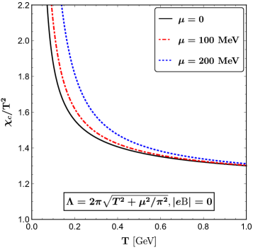
Figure 1: Variation of chiral susceptibility scaled with $T^{2}$ as a function of temperature for chemical potential 0, 100 and 200 MeV with zero magnetic field.

In Fig. 1 the chiral susceptibility scaled with temperature squared is plotted with temperature in absence of magnetic field for zero and non zero quark chemical potential. The effect of quark chemical potential is prominent in the low temperature region as can be seen from the figure. Similar plot for thermal QCD medium and zero chemical potential was obtained in Ref. Chakraborty:2002yt . For low temperature the chiral susceptibility increases rapidly for both zero and non zero chemical potential. Here we note that the increase of the chiral susceptibility in the low temperature region does not indicate the chiral phase transition. It is due to the temperature dependence of the coupling constant and for the choice of the renormalization scale Chakraborty:2002yt . At very high temperature the chiral susceptibility reaches the free value asymptotically.

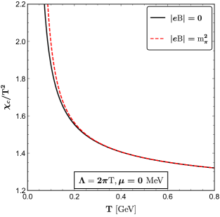
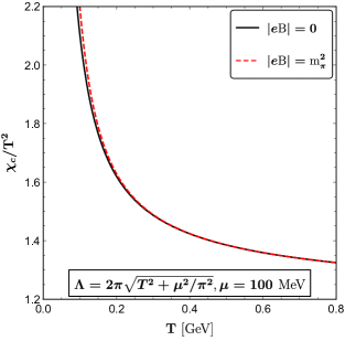
Figure 2: Variation of chiral susceptibility scaled with $T^{2}$ as a function of $T$ for magnetic field strength $|eB|=0,m_{\pi}^{2}$ with $\mu=0$ MeV (left) and $\mu=100$ MeV (right).

The variation of chiral susceptibility scaled with temperature squared for zero and finite magnetic field is plotted with temperature in Fig. 2. In the left panel of Fig. 2 we have shown the effect of weak magnetic field on the chiral susceptibility for zero quark chemical potential, whereas, the same for finite quark chemical potential is shown in the right panel. In presence of magnetic field chiral susceptibility is slightly increased than that of thermal medium in the low temperature region .Since we are working in weak magnetic field limit, the increase in susceptibility due to magnetic field is small. As temperature increases the effect of magnetic field reduces as temperature becomes the dominant scale.

It should be noted that the scale hierarchy of weakly magnetized medium is satisfied for around $T>0.14$ $GeV$ as we have considered $|eB|=m_{\pi}^{2}=0.14^{2}$ $GeV^{2}$ in Fig.2. Thus the weak field and HTL approximations are valid at high temperature.

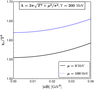
Figure 3: Scaled chiral susceptibility is plotted as a function of magnetic field strength $|eB|$ for temperature $T=0.2$ MeV and $\mu=0$ MeV and 100 MeV.

The effect of magnetic field can be seen clearly from Fig. 3 where the variation of the scaled chiral susceptibility is shown with magnetic field for fixed temperature $T=200$ MeV. Here we notice the slow increase in the chiral susceptibility with increasing magnetic field for both with and without chemical potential.

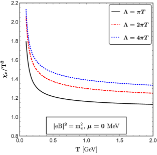
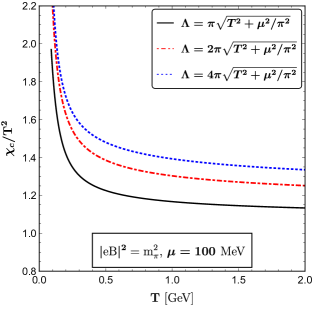
Figure 4: Variation of chiral susceptibility scaled with $T^{2}$ as a function of temperature for magnetic field strength $m_{\pi}^{2}$ for different values of renormalization scale.

In Fig. 4 the sensitivity of the chiral susceptibility with renormalization scale is shown in the presence of a constant weak magnetic field. Here chiral susceptibility scaled with $T^{2}$ is plotted with temperature for zero(left panel) and finite (right panel) chemical potential by varying renormalization scale $\Lambda$ by factor 2 around its central value $2\pi\sqrt{T^{2}+\mu^{2}/\pi^{2}}$.

Here we note that HTL approximation is valid above the phase transition temperature where the scale hierarchy $\sqrt{|q_{f}B|}<gT<T$ is maintained. We have shown the plots of chiral susceptibilities at low temperature just to show the steep increase in the plots.

VII Summary

We have investigated the effect of magnectic field on the chiral susceptibility of quark-gluon plasma within HTL approximation in presence of finite chemical potential. The general structure of effective massive fermion propagator is constructed for thermo-magnetic medium. Then the self-energy structure functions upto $\mathcal{O}[(q_{f}B)^{2}]$ in presence of chemical potential have been calculated in the weak magnetic field regime using the scale hierarchy $\sqrt{|q_{f}B|}<gT<T$. Quark condensate is computed using effective quark propagator in presence of magnetic field. Finally we obtain completely analytic expression for chiral susceptibility in hot and dense weakly magnetized QCD medium. We have subtracted the UV divergence via $\overline{MS}$ renormalization scheme. It is found that the chiral susceptibility is increased due to the presence of chemical potential as well as the background magnetic field. At high temperature the effect of magnetic field on chiral susceptibility becomes feeble.

Appendix A Structure functions

The general form of the various structure functions can be written from Eq. (4) as

$$a = \frac{1}{4}\frac{\operatorname{\text{Tr}}(\Sigma\,/\!\!\!\!P)-(P\cdot u)\operatorname{\text{Tr}}(\Sigma\,/\!\!\!\!u)}{(P\cdot u)^{2}-P^{2}},$$ (30)

$$b = \frac{1}{4}\frac{-(P\cdot u)\operatorname{\text{Tr}}(\Sigma\,/\!\!\!\!P)+P^{2}\operatorname{\text{Tr}}(\Sigma\,/\!\!\!\!u)}{(P\cdot u)^{2}-P^{2}},$$ (31)

$$c^{\prime} = -\frac{1}{4}\operatorname{\text{Tr}}(\,/\!\!\!\!u\,\Sigma\gamma_{5}),$$ (32)

$$d^{\prime} = \frac{1}{4}\operatorname{\text{Tr}}(\,/\!\!\!\!n\,\Sigma\gamma_{5}).$$ (33)

The structure functions in the presence of magnetic field depends on three Lorentz scalars

$$p_{0} = P^{\mu}u_{\mu},$$ (34)

$$p_{3} = P^{\mu}n_{\mu}=p_{z},$$ (35)

$$p_{\perp} = [-(P^{\mu}P_{\mu})^{2}+(P^{\mu}u_{\mu})^{2}-(P^{\mu}n_{\mu})^{2}]^{1/2}=(p_{1}^{2}+p_{2}^{2})^{1/2}.$$ (36)

Figure 5: Self-energy diagram for a quark in presence of background magnetic field. The double line indicates the modified quark propagator in presence of weak magnetic field.

Free quark propagator in weak magnetic field is given in Eq. (18). Now the one loop quark self-energy upto $\mathcal{O}[(q_{f}B)^{2}]$ can be written as

$$\Sigma(P) = g^{2}C_{F}\sum\!\!\!\!\!\!\!\!\!\!\int\limits_{\{K\}}\gamma_{\mu}\bigg{(}S_{0}(K)+S_{1}(K)+S_{2}(K)\bigg{)}\gamma^{\mu}\frac{1}{(K-P)^{2}}$$ (37)

$$= \Sigma_{0}+\Sigma_{1}+\Sigma_{2}.$$

From (30) structure function $a$ can be written upto $\mathcal{O}[(q_{f}B)^{2}]$ as

$$a = \frac{1}{4}\frac{\operatorname{\text{Tr}}(\Sigma_{0}\,/\!\!\!\!P)-(P\cdot u)\operatorname{\text{Tr}}(\Sigma_{0}\,/\!\!\!\!u)}{(P\cdot u)^{2}-P^{2}}+\frac{1}{4}\frac{\operatorname{\text{Tr}}(\Sigma_{2}\,/\!\!\!\!P)-(P\cdot u)\operatorname{\text{Tr}}(\Sigma_{2}\,/\!\!\!\!u)}{(P\cdot u)^{2}-P^{2}},$$ (38)

$$= a_{0}+a_{B},$$ (39)

where $a_{0}$ is purely thermal contribution $(B=0)$ and $a_{B}$ is the magnetic correction of $\mathcal{O}[(q_{f}B)^{2}]$ coming from $\Sigma_{2}$. The $\mathcal{O}[(q_{f}B)]$ corrections coming from $\Sigma_{1}$ vanish due to the trace of odd number of gamma matrices.

Similarly structure function $b$ can be written as,

$$b = \frac{1}{4}\frac{-(P\cdot u)\operatorname{\text{Tr}}(\Sigma_{0}\,/\!\!\!\!P)+P^{2}\operatorname{\text{Tr}}(\Sigma_{0}\,/\!\!\!\!u)}{(P\cdot u)^{2}-P^{2}}+\frac{1}{4}\frac{-(P\cdot u)\operatorname{\text{Tr}}(\Sigma_{2}\,/\!\!\!\!P)+P^{2}\operatorname{\text{Tr}}(\Sigma_{2}\,/\!\!\!\!u)}{(P\cdot u)^{2}-P^{2}},$$ (40)

$$= b_{0}+b_{B}.$$ (41)

The thermal part of the structure functions $a$ and $b$ can be calculated using the quark self energy diagram in Fig. 5 as Das:2017vfh

$$a_{0}(p_{0},p) = -\frac{m_{\mathrm{th}}^{2}}{p^{2}}\int\frac{d\Omega}{4\pi}\frac{p\cdot\hat{k}}{P\cdot\hat{K}},$$ (42)

$$b_{0}(p_{0},p) = \frac{m_{\mathrm{th}}^{2}}{p}\int\frac{d\Omega}{4\pi}\frac{(P\cdot u)(p\cdot\hat{k})-p^{2}}{P\cdot\hat{K}},$$ (43)

where thermal mass is given as

$$m_{\mathrm{th}}^{2} = \frac{g^{2}C_{F}T^{2}}{8}\Big{(}1+4\hat{\mu}^{2}\Big{)}$$ (44)

with $\hat{\mu}=\mu/2\pi T$ and $C_{F}=(N_{c}^{2}-1)/2N_{c}$.

Now we derive the $\mathcal{O}[(q_{f}B)^{2}]$ corrections to the structure functions $a$ and $b$. To get the expression of $a_{B}$ and $b_{B}$ we need to perform the following sum-integrations.

$$\operatorname{\text{Tr}}\big{(}{\Sigma_{2}\,/\!\!\!\!u}\big{)} = 16g^{2}C_{F}(q_{f}B)^{2}T\sum\!\!\!\!\!\!\!\!\!\!\int\limits_{\{K\}}\frac{k_{\perp}^{2}k_{0}}{(K^{2}-m_{f}^{2})^{4}\,Q^{2}}$$ (45)

$$= \frac{16}{6}g^{2}C_{F}(q_{f}B)^{2}\int\frac{k^{2}\,dk\,d\Omega}{(2\pi)^{3}}\frac{\partial^{3}}{\partial(m_{f}^{2})^{3}}\bigg{[}-\frac{k_{\perp}^{2}}{4\sqrt{k^{2}+m_{f}^{2}}}(n_{F}(\sqrt{k^{2}+m_{f}^{2}})+n_{B}(\sqrt{k^{2}+m_{f}^{2}}))\bigg{]}$$

$$\times\bigg{(}\frac{1}{p_{0}-p\cdot\hat{k}}+\frac{1}{p_{0}+p\cdot\hat{k}}\bigg{)}$$

$$= \frac{g^{2}C_{F}(q_{f}B)^{2}}{6\pi^{3}T^{2}}\Gamma(5)\frac{\partial^{3}}{\partial(y^{2})^{3}}\bigg{[}h_{5}(y)+f_{5}(y)\bigg{]}\int d\Omega\frac{\hat{k}_{\perp}^{2}}{P\cdot\hat{K}}$$

$$= \frac{g^{2}C_{F}T(q_{f}B)^{2}}{8\pi m_{f}^{3}}\int\frac{d\Omega}{4\pi}\frac{\hat{k}_{\perp}^{2}}{P\cdot\hat{K}},$$

where we have used well-known functions

$$f_{n+1}(y)=\frac{1}{\Gamma(n+1)}\int_{0}^{\infty}\frac{dx\,x^{n}}{\sqrt{x^{2}+y^{2}}}\,n_{F}\big{(}\sqrt{x^{2}+y^{2}}\big{)}$$ (46)

and

$$h_{n+1}(y)=\frac{1}{\Gamma(n+1)}\int_{0}^{\infty}\frac{dx\,x^{n}}{\sqrt{x^{2}+y^{2}}}\,n_{B}\big{(}\sqrt{x^{2}+y^{2}}\big{)},$$ (47)

which satisfy the recursion relations Bandyopadhyay:2017cle ,

$$\frac{\partial f_{n+1}}{\partial y^{2}} = -\frac{f_{n-1}}{2n},$$ (48)

$$\frac{\partial h_{n+1}}{\partial y^{2}} = -\frac{h_{n-1}}{2n}.$$ (49)

Expressions for $f_{1}(y)$ and $h_{1}(y)$ are given as

$$f_{1}(y) = \frac{\pi}{2y}+\frac{1}{2}\ln\left(\frac{y}{4\pi}\right)+\,\dotsi,$$

$$h_{1}(y) = -\frac{1}{2}\ln\left(\frac{y}{4\pi}\right)+\frac{1}{4}\aleph(z)+\,\dotsi\,,$$ (50)

where $\aleph(z)$ is defined in Eq. (76).

Now we compute the following trace as

$$\operatorname{\text{Tr}}\big{(}{\Sigma_{2}\,/\!\!\!\!P}\big{)} = X_{1}+X_{2}+X_{3}+X_{4},$$ (51)

where

$$X_{1} = -16g^{2}C_{F}(q_{f}B)^{2}\sum\!\!\!\!\!\!\!\!\!\!\int\limits_{\{K\}}\frac{k\,(p.\hat{k})}{(K^{2}-m_{f}^{2})^{3}Q^{2}}$$ (52)

$$= -8g^{2}C_{F}(q_{f}B)^{2}\int\frac{k^{2}\,dk\,d\Omega}{(2\pi)^{3}}\frac{\partial^{2}}{\partial(m_{f}^{2})^{2}}\bigg{[}\frac{k\,(p.\hat{k})}{4\,q\sqrt{k^{2}+m_{f}^{2}}}(n_{F}(\sqrt{k^{2}+m_{f}^{2}})+n_{B}(\sqrt{k^{2}+m_{f}^{2}}))\bigg{]}$$

$$\times\bigg{(}\frac{1}{p_{0}+p\cdot\hat{k}}-\frac{1}{p_{0}-p\cdot\hat{k}}\bigg{)}$$

$$= -\frac{g^{2}C_{F}(q_{f}B)^{2}}{8\pi^{3}T^{2}}\frac{\partial}{\partial y^{2}}\bigg{[}h_{1}(y)+f_{1}(y)\bigg{]}\int d\Omega\frac{p\cdot\hat{k}}{P\cdot\hat{K}}$$

$$= \frac{g^{2}C_{F}T(q_{f}B)^{2}}{8\pi m_{f}^{3}}\int\frac{d\Omega}{4\pi}\frac{p\cdot\hat{k}}{P\cdot\hat{K}}.$$

By performing similar calculations we get,

$$X_{2} = 16g^{2}C_{F}(q_{f}B)^{2}\sum\!\!\!\!\!\!\!\!\!\!\int\limits_{\{K\}}\frac{k\,\hat{k}_{3}\,p_{3}}{(K^{2}-m_{f}^{2})^{3}Q^{2}}$$ (53)

$$= -\frac{g^{2}C_{F}T(q_{f}B)^{2}}{8\pi m_{f}^{3}}\int\frac{d\Omega}{4\pi}\frac{p_{3}\,\hat{k}_{3}\,}{P\cdot\hat{K}},$$

$$X_{3} = 16g^{2}C_{F}(q_{f}B)^{2}\sum\!\!\!\!\!\!\!\!\!\!\int\limits_{\{K\}}\frac{k_{\perp}^{2}\,k_{0}\,p_{0}}{(K^{2}-m_{f}^{2})^{4}Q^{2}}$$ (54)

$$= \frac{g^{2}C_{F}T(q_{f}B)^{2}}{8\pi m_{f}^{3}}\int\frac{d\Omega}{4\pi}\frac{p_{0}\,\hat{k}_{\perp}^{2}}{P\cdot\hat{K}},$$

$$X_{4} = -16g^{2}C_{F}(q_{f}B)^{2}\sum\!\!\!\!\!\!\!\!\!\!\int\limits_{\{K\}}\frac{k_{\perp}^{2}\,k(p\cdot\hat{k})}{(K^{2}-m_{f}^{2})^{4}Q^{2}}$$ (55)

$$= -\frac{g^{2}C_{F}T(q_{f}B)^{2}}{8\pi m_{f}^{3}}\int\frac{d\Omega}{4\pi}\frac{\,\hat{k}_{\perp}^{2}(p\cdot\hat{k})}{P\cdot\hat{K}}.$$

So we obtain the expression of $a_{B}$ and $b_{B}$ as

$$a_{B} = \frac{g^{2}C_{F}T(q_{f}B)^{2}}{32\pi m_{f}^{3}}\frac{1}{p^{2}}\int\frac{d\Omega}{4\pi}\,\frac{\hat{k}_{3}^{2}\,(p\cdot\hat{k})-p_{3}\hat{k}_{3}}{P\cdot\hat{K}},$$

$$b_{B} = \frac{g^{2}C_{F}T(q_{f}B)^{2}}{32\pi m_{f}^{3}}\frac{1}{p}\int\frac{d\Omega}{4\pi}\,\,\frac{\hat{k}_{3}(P\cdot u)(\hat{p}_{3}\,-\hat{p}\cdot\hat{k}\,\hat{k}_{3})-p\,\hat{k}_{\perp}^{2}}{P\cdot\hat{K}}.$$ (56)

Other two structure functions are given as Das:2017vfh

$$c^{\prime} = -m_{\text{eff}}^{2}\int\frac{d\Omega}{4\pi}\frac{\hat{K}\cdot n}{P\cdot\hat{K}},$$

$$d^{\prime} = m_{\text{eff}}^{2}\int\frac{d\Omega}{4\pi}\frac{\hat{K}\cdot u}{P\cdot\hat{K}},$$ (57)

where the contribution comes only from $\Sigma_{1}$ term. The contributions from $\Sigma_{0}$ and $\Sigma_{2}$ vanish due the trace of odd number of gamma matrices.

Here we note that

$$m_{\text{eff}}^{2} = 4g^{2}\,C_{F}\,M_{f}^{2}(T,m_{f},q_{f}B),$$ (58)

where the thermomagnetic mass for flavor $f$ is given as

$$M_{f}^{2}(T,m_{f},q_{f}B) = \frac{q_{f}B}{16\pi^{2}}\bigg{[}-\frac{1}{4}\aleph(z)-\frac{\pi T}{2m_{f}}-\frac{\gamma_{E}}{2}\bigg{]},$$ (59)

where $\aleph(z)$ is defined in Eq. (79).

We rearrange the inverse of effective propagator in different way,

$$S_{\text{eff}}^{-1}(P) = (1+a)\,/\!\!\!\!{P}+b\,/\!\!\!\!u+c^{\prime}\,\gamma_{5}\,/\!\!\!\!u+d^{\prime}\,\gamma_{5}\,/\!\!\!\!n-m_{f}\,\mathbb{I}$$ (60)

$$= c\,p_{0}\,\gamma_{0}-dp_{i}\,\gamma_{i}+c^{\prime}\,\gamma_{5}\,/\!\!\!\!u+d^{\prime}\,\gamma_{5}\,/\!\!\!\!n-m_{f}\,\mathbb{I},$$

where

$$c = 1+(a_{0}+\frac{b_{0}}{p_{0}})+(a_{B}+\frac{b_{B}}{p_{0}})=1-a^{\prime}_{0}-a^{\prime}_{B},$$

$$d = 1+a_{0}+a_{B},$$ (61)

with

$$a_{0} = \frac{m_{\text{th}}^{2}}{p^{2}}(1-\mathcal{T}_{p}),$$

$$a^{\prime}_{0} = \frac{m_{\text{th}}^{2}}{p_{0}^{2}}\mathcal{T}_{p},$$

$$a_{B} = \frac{m^{\prime 2}_{\text{eff}}}{6p^{2}}\bigg{(}1-\frac{3\,p_{3}^{2}}{p^{2}}\bigg{)}\bigg{(}\frac{3\,p_{0}^{2}}{p^{2}}(1-\mathcal{T}_{p})-2+3\mathcal{T}_{p}\bigg{)},$$

$$a^{\prime}_{B} = \frac{m^{\prime 2}_{\text{eff}}}{2p_{0}^{2}}\bigg{(}3\,\frac{p_{0}^{2}\,p_{3}^{2}}{p^{4}}(1-\mathcal{T}_{p})+\mathcal{T}_{p}+\frac{1}{p^{2}}\bigg{(}p_{3}^{2}\,\mathcal{T}_{p}-p_{0}^{2}(1-\mathcal{T}_{p})\bigg{)}\bigg{)},$$

$$c^{\prime} = \frac{p_{3}\,m_{\text{eff}}^{2}}{p^{2}}(1-\mathcal{T}_{p}),$$

$$d^{\prime} = \frac{m_{\text{eff}}^{2}}{p_{0}}\mathcal{T}_{p}.$$ (62)

We expressed all the structure functions in terms of

$$\mathcal{T}_{p} = \int\frac{d\Omega}{4\pi}\frac{p_{0}}{p_{0}-p\cdot\hat{k}}.$$ (63)

Here we have defined

$$m^{\prime 2}_{\text{eff}} = \frac{g^{2}C_{F}(q_{f}B)^{2}T}{32\,\pi\,m_{f}^{3}}$$ (64)

with $C_{F}=(N_{c}^{2}-1)/2N_{c}$. We can see that $m^{\prime 2}_{\text{eff}}$ and $m_{\text{eff}}^{2}$ diverge when current quark mass vanishes ($m_{f}\rightarrow 0$). It is regulated by thermal mass $m_{th}$ of the fermion as discussed in Refs. Kapusta:2006pm ; Ayala:2014uua .

Appendix B Sum-integrals

The dimensionally regularized sum integrals are defined as

$$\sum\!\!\!\!\!\!\!\!\!\!\int\limits_{\{P\}} = \left(\frac{e^{\gamma_{E}}\Lambda^{2}}{4\pi}\right)^{\epsilon}T\sum\limits_{\begin{subarray}{c}p_{0}=(2n+1)\pi Ti+\mu\end{subarray}}\int\frac{d^{d-2\epsilon}p}{(2\pi)^{d-2\epsilon}},$$ (65)

where $\Lambda$ can be identified as the $\overline{MS}$ renormalization scale which also introduces the factor $\left(\frac{e^{\gamma_{E}}}{4\pi}\right)^{\epsilon}$ along with it where $\gamma_{E}$ is the Euler-Mascheroni constant.

The sum integrals are related by the following equations.

$$\sum\!\!\!\!\!\!\!\!\!\!\int\limits_{\{P\}}\frac{1}{P^{4}}=-\frac{d-2}{2}\sum\!\!\!\!\!\!\!\!\!\!\int\limits_{\{P\}}\frac{1}{p^{2}P^{2}},$$ (66)

$$\sum\!\!\!\!\!\!\!\!\!\!\int\limits_{\{P\}}\frac{1}{p^{2}P^{4}}=-\frac{d-4}{2}\sum\!\!\!\!\!\!\!\!\!\!\int\limits_{\{P\}}\frac{1}{p^{4}P^{2}}.$$ (67)

B.1 One-loop sum integrals

We list the fermionic sum-integrals as Bandyopadhyay:2017cle ; Chakraborty:2002yt

$$\sum\!\!\!\!\!\!\!\!\!\!\int\limits_{\{P\}}\frac{1}{P^{2}} = \frac{T^{2}}{24}\left(\frac{\Lambda}{4\pi T}\right)^{2\epsilon}\left[1+12\hat{\mu}^{2}\right],$$ (68)

$$\sum\!\!\!\!\!\!\!\!\!\!\int\limits_{\{P\}}\frac{1}{P^{4}} = \frac{1}{\left(4\pi\right)^{2}}\left(\frac{\Lambda}{4\pi T}\right)^{2\epsilon}\Bigg{[}\frac{1}{\epsilon}-\aleph(z)\Bigg{]},$$ (69)

$$\sum\!\!\!\!\!\!\!\!\!\!\int\limits_{\{P\}}\frac{p_{3}^{2}}{p^{2}P^{4}} = \frac{1}{3\left(4\pi\right)^{2}}\left(\frac{\Lambda}{4\pi T}\right)^{2\epsilon}\Bigg{[}\frac{1}{\epsilon}+\frac{2}{3}-\aleph(z)\Bigg{]},$$ (70)

$$\sum\!\!\!\!\!\!\!\!\!\!\int\limits_{\{P\}}\frac{1}{P^{6}} = \frac{1}{(2\pi)^{4}}\left(\frac{\Lambda}{4\pi T}\right)^{2\epsilon}\frac{\gimel(z)}{32T^{2}},$$ (71)

$$\sum\!\!\!\!\!\!\!\!\!\!\int\limits_{\{P\}}\frac{1}{p^{4}P^{2}} = -\frac{1}{(2\pi)^{4}}\left(\frac{\Lambda}{4\pi T}\right)^{2\epsilon}\frac{\gimel(z)}{4T^{2}},$$ (72)

$$\sum\!\!\!\!\!\!\!\!\!\!\int\limits_{\{P\}}\frac{1}{p^{2}P^{4}} = -\frac{1}{(2\pi)^{4}}\left(\frac{\Lambda}{4\pi T}\right)^{2\epsilon}\frac{\gimel(z)}{8T^{2}},$$ (73)

$$\sum\!\!\!\!\!\!\!\!\!\!\int\limits_{\{P\}}\frac{p_{3}^{2}}{p^{2}P^{6}} = \frac{1}{(2\pi)^{4}}\left(\frac{\Lambda}{4\pi T}\right)^{2\epsilon}\frac{\gimel(z)}{96T^{2}},$$ (74)

$$\sum\!\!\!\!\!\!\!\!\!\!\int\limits_{\{P\}}\frac{p_{3}^{2}}{p^{4}P^{4}} = -\frac{1}{(2\pi)^{4}}\left(\frac{\Lambda}{4\pi T}\right)^{2\epsilon}\frac{\gimel(z)}{24T^{2}}.$$ (75)

Here we list the frequently used functions in the sum-integrals

$$\aleph(z) \equiv \Psi(z)+\Psi(z^{*}),$$ (76)

$$\gimel(z) \equiv \frac{d^{2}}{dz^{2}}\Big{(}\Psi(z)+\Psi(z^{*})\Big{)},$$ (77)

where $z$ is a general complex number, here $z=1/2-i\hat{\mu}$. $\zeta$ and $\Psi$ denote the Riemann Zeta function and the digamma function respectively. The digamma function can be written as

$$\Psi(z)\equiv\frac{\Gamma^{\prime}(z)}{\Gamma(z)}.$$ (78)

We write the functional form of $\aleph(1/2-i\hat{\mu})$ and $\gimel(1/2-i\hat{\mu})$ for small $\hat{\mu}$ below.

$$\aleph(z) = -2\gamma_{E}-4\ln 2+14\zeta(3)\hat{\mu}^{2}-62\zeta(5)\hat{\mu}^{4}+254\zeta(7)\hat{\mu}^{6}+{\cal O}(\hat{\mu}^{8}),$$ (79)

$$\gimel(z) = -4\bigg{[}7\zeta(3)-186\zeta(5)\hat{\mu}^{2}+1905\zeta(7)\hat{\mu}^{4}-14308\zeta(9)\hat{\mu}^{6}\bigg{]}+\mathcal{O}(\hat{\mu}^{8}).$$ (80)

B.2 One-loop HTL sum integrals used in the magnetic case

We also need one-loop HTL sum integrals which involve the angular average defined earlier in Eq. (63). For brevity, henceforth we will use the notation $c=\cos\theta$ for single angular average and $c_{i}=\cos\theta_{i}$ for multiple angular averages. We list the sum integrals below:

$$\sum\!\!\!\!\!\!\!\!\!\!\int\limits_{\{P\}}\frac{1}{P^{4}}\mathcal{T}_{p} = \frac{d-4}{d-5}\sum\!\!\!\!\!\!\!\!\!\!\int\limits_{\{P\}}\frac{1}{P^{4}}$$ (81)

$$\sum\!\!\!\!\!\!\!\!\!\!\int\limits_{\{P\}}\frac{1}{p^{2}P^{4}}\mathcal{T}_{p} = \Big{(}\Delta_{1}-\frac{d-4}{2}\Delta_{2}\Big{)}\sum\!\!\!\!\!\!\!\!\!\!\int\limits_{\{P\}}\frac{1}{p^{4}P^{2}},,$$ (82)

$$\sum\!\!\!\!\!\!\!\!\!\!\int\limits_{\{P\}}\frac{p_{3}^{2}}{p^{2}P^{4}}\mathcal{T}_{p} = \bigg{(}\frac{d-4}{d-2}(1+\Delta_{0})+\frac{2}{d-2}\Delta_{3}^{\prime}\bigg{)}\Delta_{3}\sum\!\!\!\!\!\!\!\!\!\!\int\limits_{\{P\}}\frac{1}{P^{4}}$$ (83)

$$\sum\!\!\!\!\!\!\!\!\!\!\int\limits_{\{P\}}\frac{\mathcal{T}_{p}^{2}}{p^{2}p_{0}^{2}P^{2}} = \Delta_{4}\sum\!\!\!\!\!\!\!\!\!\!\int\limits_{\{P\}}\frac{1}{p^{4}P^{2}},,$$ (84)

$$\sum\!\!\!\!\!\!\!\!\!\!\int\limits_{\{P\}}\frac{p_{3}^{2}}{p^{4}P^{4}}\mathcal{T}_{p} = \Big{(}\Delta_{1}-\frac{d-4}{2}\Delta_{2}\Big{)}\Delta_{3}\sum\!\!\!\!\!\!\!\!\!\!\int\limits_{\{P\}}\frac{1}{p^{4}P^{2}},$$ (85)

$$\sum\!\!\!\!\!\!\!\!\!\!\int\limits_{\{P\}}\frac{1}{p_{0}^{2}P^{4}}\mathcal{T}_{p}^{2} = \Delta_{5}\sum\!\!\!\!\!\!\!\!\!\!\int\limits_{\{P\}}\frac{1}{p^{4}P^{2}},$$ (86)

$$\sum\!\!\!\!\!\!\!\!\!\!\int\limits_{\{P\}}\frac{p_{3}^{2}}{p^{4}P^{4}}\mathcal{T}_{p}^{2} = \Delta_{3}\Delta_{6}\sum\!\!\!\!\!\!\!\!\!\!\int\limits_{\{P\}}\frac{1}{p^{4}P^{2}},$$ (87)

$$\sum\!\!\!\!\!\!\!\!\!\!\int\limits_{\{P\}}\frac{p_{3}^{2}}{p^{2}p_{0}^{2}P^{4}}\mathcal{T}_{p}^{2} = \Delta_{3}\Delta_{5}\sum\!\!\!\!\!\!\!\!\!\!\int\limits_{\{P\}}\frac{1}{p^{4}P^{2}},$$ (88)

where $\Delta$’s are the various angular averages which we list below. The symbol $\langle\rangle_{c}$ in the angular averages depicts the standard definition used in Ref. Andersen:2002ey .

$$\Delta_{0} = \left\langle\frac{c^{2}}{1-c^{2}}\right\rangle_{c}=-\frac{1}{2\epsilon}+\mathcal{O}[\epsilon]^{3},$$ (89)

$$\Delta_{1} = \left\langle\frac{c^{6-d}-c^{2}}{(1-c^{2})^{2}}\right\rangle_{c}=\frac{1}{4\epsilon}-\frac{1}{4}+\ln 2+\epsilon\bigg{[}-\frac{3}{4}+\frac{\pi^{2}}{6}+(\ln 2)^{2}-2\ln 2\bigg{]}+\mathcal{O}[\epsilon]^{2},$$ (90)

$$\Delta_{2} = \left\langle\frac{1}{1-c^{2}}\right\rangle_{c}=-\frac{1}{2\epsilon}+1+\mathcal{O}[\epsilon],$$ (91)

$$\Delta_{3} = \left\langle c^{2}\right\rangle_{c}=\frac{1}{3}+\frac{2\epsilon}{9}+\mathcal{O}[\epsilon]^{2},$$ (92)

$$\Delta_{3}^{\prime} = \left\langle\frac{1-c^{4-d}}{(1-c^{2})^{2}}\right\rangle_{c}=-\frac{1}{4\epsilon}+\frac{1}{4}+\frac{3\epsilon}{4}-\frac{3\epsilon^{2}}{4}+\mathcal{O}[\epsilon]^{3},$$ (93)

$$\Delta_{4} = \left\langle\frac{1-c_{1}^{6-d}}{(c_{1}^{2}-c_{2}^{2})(1-c_{1}^{2})}+c_{1}\leftrightarrow c_{2}\right\rangle_{c_{1},c_{2}}=\frac{1}{12}\bigg{[}24\ln 2-\pi^{2}\bigg{]}+\mathcal{O}[\epsilon],$$ (94)

$$\Delta_{5} = \left\langle\frac{c_{1}^{6-d}-c_{1}^{2}}{(c_{1}^{2}-c_{2}^{2})(1-c_{1}^{2})^{2}}-\frac{d-4}{2}\frac{1}{(c_{1}^{2}-c_{2}^{2})(1-c_{1}^{2})}+c_{1}\leftrightarrow c_{2}\right\rangle_{c_{1},c_{2}}=\frac{1}{24}\bigg{[}6-\pi^{2}\bigg{]}+\mathcal{O}[\epsilon],$$ (95)

$$\Delta_{6} = \left\langle\frac{1-2c_{1}^{2}+c_{1}^{8-d}}{(c_{1}^{2}-c_{2}^{2})(1-c_{1}^{2})^{2}}-\frac{d-4}{2}\frac{1}{(c_{1}^{2}-c_{2}^{2})(1-c_{1}^{2})}+c_{1}\leftrightarrow c_{2}\right\rangle_{c_{1},c_{2}}=\frac{1}{8}\bigg{[}2-\pi^{2}+16\ln 2\bigg{]}+\mathcal{O}[\epsilon].$$

Using the expressions of angular averages we obtain the results of HTL sum integrals for magnetic case as

$$\sum\!\!\!\!\!\!\!\!\!\!\int\limits_{\{P\}}\frac{1}{P^{4}}\mathcal{T}_{p} = \frac{1}{2\left(4\pi\right)^{2}}\left(\frac{\Lambda}{4\pi T}\right)^{2\epsilon}\Bigg{[}\frac{1}{\epsilon}+1-\aleph(z)\Bigg{]},$$ (97)

$$\sum\!\!\!\!\!\!\!\!\!\!\int\limits_{\{P\}}\frac{1}{p^{2}P^{4}}\mathcal{T}_{p} = -\frac{1}{(2\pi)^{4}}\left(\frac{\Lambda}{4\pi T}\right)^{2\epsilon}\frac{\gimel(z)}{16T^{2}}\Big{(}-1+4\ln 2\Big{)},$$ (98)

$$\sum\!\!\!\!\!\!\!\!\!\!\int\limits_{\{P\}}\frac{p_{3}^{2}}{p^{2}P^{4}}\mathcal{T}_{p} = \frac{1}{6\left(4\pi\right)^{2}}\left(\frac{\Lambda}{4\pi T}\right)^{2\epsilon}\Bigg{[}\frac{1}{\epsilon}+\frac{5}{3}-\aleph(z)\Bigg{]},$$ (99)

$$\sum\!\!\!\!\!\!\!\!\!\!\int\limits_{\{P\}}\frac{1}{p^{2}p_{0}^{2}P^{2}}\mathcal{T}_{p}^{2} = \frac{1}{(2\pi)^{4}}\!\left(\frac{\Lambda}{4\pi T}\right)^{2\epsilon}\frac{\gimel(z)}{48T^{2}}\Big{(}\pi^{2}-24\ln 2\Big{)},$$ (100)

$$\sum\!\!\!\!\!\!\!\!\!\!\int\limits_{\{P\}}\frac{p_{3}^{2}}{p^{4}P^{4}}\mathcal{T}_{p} = -\frac{1}{(2\pi)^{4}}\left(\frac{\Lambda}{4\pi T}\right)^{2\epsilon}\frac{\gimel(z)}{48T^{2}}\Big{(}-1+4\ln 2\Big{)},$$ (101)

$$\sum\!\!\!\!\!\!\!\!\!\!\int\limits_{\{P\}}\frac{1}{p_{0}^{2}P^{4}}\mathcal{T}_{p}^{2} = \frac{1}{(2\pi)^{4}}\left(\frac{\Lambda}{4\pi T}\right)^{2\epsilon}\frac{\gimel(z)}{96T^{2}}\Big{(}\pi^{2}-6\Big{)},$$ (102)

$$\sum\!\!\!\!\!\!\!\!\!\!\int\limits_{\{P\}}\frac{p_{3}^{2}}{p^{4}P^{4}}\mathcal{T}_{p}^{2} = \frac{1}{(2\pi)^{4}}\left(\frac{\Lambda}{4\pi T}\right)^{2\epsilon}\frac{\gimel(z)}{96T^{2}}\Big{(}-2+\pi^{2}-16\ln 2\Big{)},$$ (103)

$$\sum\!\!\!\!\!\!\!\!\!\!\int\limits_{\{P\}}\frac{p_{3}^{2}}{p^{2}p_{0}^{2}P^{4}}\mathcal{T}_{p}^{2} = \frac{1}{(2\pi)^{4}}\left(\frac{\Lambda}{4\pi T}\right)^{2\epsilon}\frac{\gimel(z)}{288T^{2}}\Big{(}\pi^{2}-6\Big{)}.$$ (104)

References

• (1) Y. Aoki, G. Endrodi, Z. Fodor, S. D. Katz and K. K. Szabo, Nature 443, 675-678 (2006) doi:10.1038/nature05120 [arXiv:hep-lat/0611014 [hep-lat]].
• (2) T. Bhattacharya, M. I. Buchoff, N. H. Christ, H. T. Ding, R. Gupta, C. Jung, F. Karsch, Z. Lin, R. D. Mawhinney and G. McGlynn, et al. Phys. Rev. Lett. 113, no.8, 082001 (2014) doi:10.1103/PhysRevLett.113.082001 [arXiv:1402.5175 [hep-lat]].
• (3) K. Fukushima, Phys. Lett. B 591, 277-284 (2004) doi:10.1016/j.physletb.2004.04.027 [arXiv:hep-ph/0310121 [hep-ph]].
• (4) C. Ratti, M. A. Thaler and W. Weise, Phys. Rev. D 73, 014019 (2006) doi:10.1103/PhysRevD.73.014019 [arXiv:hep-ph/0506234 [hep-ph]].
• (5) Z. Fang, Y. L. Wu and L. Zhang, Phys. Rev. D 99, no.3, 034028 (2019) doi:10.1103/PhysRevD.99.034028 [arXiv:1810.12525 [hep-ph]].
• (6) C. S. Fischer, Phys. Rev. Lett. 103, 052003 (2009) doi:10.1103/PhysRevLett.103.052003 [arXiv:0904.2700 [hep-ph]].
• (7) J. Braun, L. M. Haas, F. Marhauser and J. M. Pawlowski, Phys. Rev. Lett. 106, 022002 (2011) doi:10.1103/PhysRevLett.106.022002 [arXiv:0908.0008 [hep-ph]].
• (8) F. Karsch and E. Laermann, Phys. Rev. D 50, 6954-6962 (1994) doi:10.1103/PhysRevD.50.6954 [arXiv:hep-lat/9406008 [hep-lat]].
• (9) C. Bernard et al. [MILC], Phys. Rev. D 71, 034504 (2005) doi:10.1103/PhysRevD.71.034504 [arXiv:hep-lat/0405029 [hep-lat]].
• (10) M. Cheng, N. H. Christ, S. Datta, J. van der Heide, C. Jung, F. Karsch, O. Kaczmarek, E. Laermann, R. D. Mawhinney and C. Miao, et al. Phys. Rev. D 74, 054507 (2006) doi:10.1103/PhysRevD.74.054507 [arXiv:hep-lat/0608013 [hep-lat]].
• (11) L. K. Wu, X. Q. Luo and H. S. Chen, Phys. Rev. D 76, 034505 (2007) doi:10.1103/PhysRevD.76.034505 [arXiv:hep-lat/0611035 [hep-lat]].
• (12) S. Digal, E. Laermann and H. Satz, Eur. Phys. J. C 18, 583-586 (2001) doi:10.1007/s100520000538 [arXiv:hep-ph/0007175 [hep-ph]].
• (13) P. Chakraborty, M. G. Mustafa and M. H. Thoma, Phys. Rev. D 67, 114004 (2003) doi:10.1103/PhysRevD.67.114004 [arXiv:hep-ph/0210159 [hep-ph]].
• (14) A. V. Smilga and J. J. M. Verbaarschot, Phys. Rev. D 54, 1087-1093 (1996) doi:10.1103/PhysRevD.54.1087 [arXiv:hep-ph/9511471 [hep-ph]].
• (15) P. Zhuang, J. Hufner and S. P. Klevansky, Nucl. Phys. A 576, 525-552 (1994) doi:10.1016/0375-9474(94)90743-9.
• (16) C. Sasaki, B. Friman and K. Redlich, Phys. Rev. D 75, 074013 (2007) doi:10.1103/PhysRevD.75.074013 [arXiv:hep-ph/0611147 [hep-ph]].
• (17) D. Blaschke, A. Holl, C. D. Roberts and S. M. Schmidt, Phys. Rev. C 58, 1758-1766 (1998) doi:10.1103/PhysRevC.58.1758 [arXiv:nucl-th/9803030 [nucl-th]].
• (18) D. E. Kharzeev, Prog. Part. Nucl. Phys. 75, 133-151 (2014) doi:10.1016/j.ppnp.2014.01.002 [arXiv:1312.3348 [hep-ph]].
• (19) K. Fukushima, Lect. Notes Phys. 871, 241-259 (2013) doi:10.1007/978-3-642-37305-3_9 [arXiv:1209.5064 [hep-ph]].
• (20) G. S. Bali, F. Bruckmann, G. Endrodi, Z. Fodor, S. D. Katz, S. Krieg, A. Schafer and K. K. Szabo, JHEP 02, 044 (2012) doi:10.1007/JHEP02(2012)044 [arXiv:1111.4956 [hep-lat]].
• (21) A. Bandyopadhyay, B. Karmakar, N. Haque and M. G. Mustafa, Phys. Rev. D 100, no.3, 034031 (2019) doi:10.1103/PhysRevD.100.034031 [arXiv:1702.02875 [hep-ph]].
• (22) B. Karmakar, R. Ghosh, A. Bandyopadhyay, N. Haque and M. G. Mustafa, Phys. Rev. D 99, no.9, 094002 (2019) doi:10.1103/PhysRevD.99.094002 [arXiv:1902.02607 [hep-ph]].
• (23) S. Rath and B. K. Patra, JHEP 12, 098 (2017) doi:10.1007/JHEP12(2017)098 [arXiv:1707.02890 [hep-th]].
• (24) K. Hattori, X. G. Huang, D. H. Rischke and D. Satow, Phys. Rev. D 96, no.9, 094009 (2017) doi:10.1103/PhysRevD.96.094009 [arXiv:1708.00515 [hep-ph]].
• (25) K. Tuchin, J. Phys. G 39, 025010 (2012) doi:10.1088/0954-3899/39/2/025010 [arXiv:1108.4394 [nucl-th]].
• (26) K. Hattori, S. Li, D. Satow and H. U. Yee, Phys. Rev. D 95, no.7, 076008 (2017) doi:10.1103/PhysRevD.95.076008 [arXiv:1610.06839 [hep-ph]].
• (27) M. Kurian, Phys. Rev. D 102, no.1, 014041 (2020) doi:10.1103/PhysRevD.102.014041 [arXiv:2005.04247 [nucl-th]].
• (28) M. Kurian, V. Chandra and S. K. Das, Phys. Rev. D 101, no.9, 094024 (2020) doi:10.1103/PhysRevD.101.094024 [arXiv:2002.03325 [nucl-th]].
• (29) M. Kurian, S. Mitra, S. Ghosh and V. Chandra, Eur. Phys. J. C 79, no.2, 134 (2019) doi:10.1140/epjc/s10052-019-6649-z [arXiv:1805.07313 [nucl-th]].
• (30) M. Kurian and V. Chandra, Phys. Rev. D 97, no.11, 116008 (2018) doi:10.1103/PhysRevD.97.116008 [arXiv:1802.07904 [nucl-th]].
• (31) K. Tuchin, Adv. High Energy Phys. 2013, 490495 (2013) doi:10.1155/2013/490495 [arXiv:1301.0099 [hep-ph]].
• (32) K. Tuchin, Phys. Rev. C 88, 024910 (2013) doi:10.1103/PhysRevC.88.024910 [arXiv:1305.0545 [nucl-th]].
• (33) A. Bandyopadhyay, C. A. Islam and M. G. Mustafa, Phys. Rev. D 94, no.11, 114034 (2016) doi:10.1103/PhysRevD.94.114034 [arXiv:1602.06769 [hep-ph]].
• (34) S. Ghosh and V. Chandra, Phys. Rev. D 98, no.7, 076006 (2018) doi:10.1103/PhysRevD.98.076006 [arXiv:1808.05176 [hep-ph]].
• (35) A. Das, N. Haque, M. G. Mustafa and P. K. Roy, Phys. Rev. D 99, no.9, 094022 (2019) doi:10.1103/PhysRevD.99.094022 [arXiv:1903.03528 [hep-ph]].
• (36) M. Hasan, B. Chatterjee and B. K. Patra, Eur. Phys. J. C 77, no.11, 767 (2017) doi:10.1140/epjc/s10052-017-5346-z [arXiv:1703.10508 [hep-ph]].
• (37) B. Singh, L. Thakur and H. Mishra, Phys. Rev. D 97, no.9, 096011 (2018) doi:10.1103/PhysRevD.97.096011 [arXiv:1711.03071 [hep-ph]].
• (38) R. Ghosh, B. Karmakar and M. G. Mustafa, Phys. Rev. D 101, no.5, 056007 (2020) doi:10.1103/PhysRevD.101.056007 [arXiv:1911.00744 [hep-ph]].
• (39) I. A. Shovkovy, Lect. Notes Phys. 871, 13-49 (2013) doi:10.1007/978-3-642-37305-3_2 [arXiv:1207.5081 [hep-ph]].
• (40) G. S. Bali, F. Bruckmann, G. Endrodi, Z. Fodor, S. D. Katz and A. Schafer, Phys. Rev. D 86, 071502 (2012) doi:10.1103/PhysRevD.86.071502 [arXiv:1206.4205 [hep-lat]].
• (41) A. Das, D. Kumar and H. Mishra, Phys. Rev. D 100, no.9, 094030 (2019) doi:10.1103/PhysRevD.100.094030 [arXiv:1907.12332 [hep-ph]].
• (42) A. Bzdak and V. Skokov, Anisotropy of photon production: initial eccentricity or magnetic field, Phys. Rev. Lett.  110, no. 19, 192301 (2013) doi:10.1103/PhysRevLett.110.192301 [arXiv:1208.5502 [hep-ph]].
• (43) L. McLerran and V. Skokov, Comments About the Electromagnetic Field in Heavy-Ion Collisions, Nucl. Phys. A 929 (2014) 184 doi:10.1016/j.nuclphysa.2014.05.008 [arXiv:1305.0774 [hep-ph]].
• (44) A. Das, A. Bandyopadhyay, P. K. Roy and M. G. Mustafa, Phys. Rev. D 97, no.3, 034024 (2018)
• (45) A. Das and N. Haque, Phys. Rev. D 101, no.7, 074033 (2020)
• (46) T. K. Chyi, C. W. Hwang, W. F. Kao, G. L. Lin, K. W. Ng and J. J. Tseng, Phys. Rev. D 62, 105014 (2000)
• (47) A. Ayala, C. A. Dominguez, S. Hernandez-Ortiz, L. A. Hernandez, M. Loewe, D. Manreza Paret and R. Zamora, Phys. Rev. D 98, no.3, 031501 (2018)
• (48) J. Beringer et al. [Particle Data Group], Phys. Rev. D 86, 010001 (2012) doi:10.1103/PhysRevD.86.010001
• (49) J. I. Kapusta and C. Gale, Finite-temperature field theory: Principles and applications,
• (50) A. Ayala, J. J. Cobos-Martínez, M. Loewe, M. E. Tejeda-Yeomans and R. Zamora, Phys. Rev. D 91, no.1, 016007 (2015) doi:10.1103/PhysRevD.91.016007 [arXiv:1410.6388 [hep-ph]].
• (51) J. O. Andersen, E. Braaten, E. Petitgirard, and M. Strickland, Phys. Rev. D 66 (2002) 085016.