Performance Analysis of Dual-Hop Relaying for THz-RF Wireless Link with Asymmetrical Fading

Abstract

Terahertz (THz) frequency bands can be promising for data transmissions between the core network and access points (AP) for next-generation wireless systems. In this paper, we analyze the performance of a dual-hop THz-RF wireless system where an AP facilitates data transmission between a core network and user equipment (UE). We consider a generalized model for the end-to-end channel with independent and not identically distributed (i.ni.d.) fading model for THz and RF links using the $\alpha$-$\mu$ distribution, the THz link with pointing errors, and asymmetrical relay position. We derive a closed-form expression of the cumulative distribution function (CDF) of the end-to-end signal to noise ratio (SNR) for the THz-RF link, which is valid for continuous values of $\mu$ for a generalized performance analysis over THz fading channels. Using the derived CDF, we analyze the performance of THz-RF relayed system using decode-and-forward (DF) protocol by deriving analytical expressions of diversity order, moments of SNR, ergodic capacity, and average BER in terms of system parameters. We also analyze the considered system with an i.i.d. model, and develop simplified performance to provide insight on the system behavior analytically under various practically relevant scenarios. Simulation and numerical analysis show significant effect of fading parameters of the THz link and a nominal effect of normalized beam-width on the performance of the relay-assisted THz-RF system.

I Introduction

Network densification is a potential technology to support the widespread proliferation of high data rate applications for a large number of devices [2, 3, 4]. This densification can be realized by adding more cell sites, including radio access networks (RAN), macro sites, small cell deployments, the cell-free architecture, and the use of novel Terahertz (THz) spectrum. The THz can provide tremendously high, unlicensed bandwidth which can be central to ubiquitous wireless communications in beyond-5G or sixth-generation (6G) networks [5, 6, 7]. Generally, the devices are connected over the radio frequency (RF) to a nearby access point (AP), which transports data to the core network through a high-speed back-haul link. The wire-line back-haul may consist of digital subscriber lines (DSL) and optical fiber. However, wire-line links might not be feasible in some adverse situations [8]. In contrast to the wireless back-haul link over the RF frequencies, THz wireless systems can be a promising alternative for high data rate transmission between the core and AP. Until the transition to a complete THz system, the communication link between a user and the AP will continue on the conventional low-frequency RF transmissions. It is desirable to evaluate the performance of a heterogeneous THz-RF link for the next generation of wireless networks.

The THz link suffers from pointing errors when there is a misalignment between transmitter and receiver antenna beams at higher frequencies besides the signal fading and significantly higher path loss. Recently, the use of THz for wireless communications is gaining research interests [9, 10, 11, 12, 13, 14, 15, 16, 17, 18, 19, 20, 21, 22, 23, 24, 25, 26, 27, 28, 29, 30]. The authors in [9] proposed a prototype of a wireless local area network at $0.34$ THz frequency band. The authors in [10] have analyzed the ergodic capacity and outage probability for a single-link THz system by deriving distribution functions for the combined effect of pointing errors[31] and $\alpha$-$\mu$ fading [32]. The $\alpha$-$\mu$ is a generalized model that includes other fading models as a particular case, and it is well studied in the RF context. Recently, the authors in [11] have derived the average bit-error-rate (BER) and the outage probability of a mixed THz-RF link with decode and forward (DF) relaying. However, derived distribution functions are valid only for integer values of the fading parameter $\mu$. Further, the short term fading is assumed to be independent and identically distributed (i.i.d) with the same parameters $\alpha$ and $\mu$ for both the THz and RF channels. The i.i.d. model might not be possible considering two technologies operating over the different spectrum. Moreover, there is no analysis available in the open literature for the average signal to noise ratio (SNR) and ergodic rate performance for the THz-RF relaying. Performance bounds on the outage probability, average SNR, ergodic rate, and average BER are desirable for real-time tuning of system parameters for efficient deployment of the THz-RF system.

In this paper, we analyze the performance of a THz-RF link with DF relaying for data transmission between the central processing unit of a core network and a user through an AP in a wireless network over $\alpha$-$\mu$ fading channels. The major contributions of the paper are as follows:

• We consider a generalized model for the end-to-end channel with independent and not identically distributed (i.ni.d.) fading model for THz and RF links, the THz link with pointing errors, and asymmetrical relay position between the source and destination.

• We derive a closed-form expression of the cumulative distribution function (CDF) for the SNR of the THz link using the combined effect of $\alpha$-$\mu$ fading and pointing errors. The derived CDF is also valid for non-integer values of $\mu$ for a generalized performance analysis over THz fading channels.

• We analyze the performance of the THz-RF relayed system by deriving analytical expressions of diversity order, moments of SNR, ergodic capacity, and average BER in terms of system parameters. The derived expressions are expressed in well-known mathematical functions, and can be evaluated using standard computational software.

• Considering the i.i.d. model of the short term fading using the same $\alpha$ and $\mu$ parameters for THz and RF links, we derive analytical expressions on the average SNR, ergodic capacity, and average BER of the relay-assisted system. The i.i.d. model simplifies the derived analytical expressions and provide insight on the system performance analytically. The average SNR and ergodic capacity performance of the THz-RF system with the i.i.d. model is accepted for presentation in the conference version of this paper [1].

• We validate the analytical results using numerical and Monte Carlo simulations. The computer simulations show a significant effect of fading parameters of the THz link and a nominal effect of normalized beam-width on the performance of the relay-assisted THz-RF system.

I-A Related Work

The THz spectrum can provide tremendously high unlicensed bandwidth, which can be a catalyst for next-generation wireless technologies. However, the path-loss in the THz band is higher due to molecular absorption of the signal at extremely small wavelengths [14, 15, 16, 17]. In [14], the authors have presented an experimental characterization of the THz channel ($300$-$320$ GHz). The effect of scattering and absorption losses on THz wavelengths in the absence of white noise were examined in [15]. Signal prorogation in the indoor environment with the blockage effects by the walls and human bodies was analyzed in [16]. A spatial modulation technique to mitigate the path-loss at THz frequencies using the properties of densely packed configurable arrays of nano-antennas was presented in [17].

In addition to the path loss, the THz transmissions undergo signal fading due to the multi-path propagation [10, 11, 12, 13, 18, 14, 15, 19, 16, 20]. The authors in [12] used the radiative transfer theory with molecular absorption to present a propagation channel model for short-distance THz transmissions. In [13], an experimental channel model in an indoor environment at $300$ GHz frequency for line-of-sight (LOS) and non-LOS scenarios was proposed. The authors in [18] have considered $m$-Nakagami fading to model a 4$\times$4 THz multiple-input multiple-output (MIMO) system. A shadowed Beaulieu-Xie (BX) fading model was suggested in [19]. The authors in [20] used advanced channel characteristics such as spherical wavefront, time-variant velocities, and space-time frequencies to model a three-dimensional non-stationary channel for millimeter-wave and THz transmissions. Recently, the generalized $\alpha$-$\mu$ and fluctuating two ray (FTR) fading models are employed for THz channels due to their tractability in performance analysis [10] [33].

As is for any communication systems, THz systems are impacted by noise, interference [21, 22, 23, 24], and pointing errors [11, 10, 25, 26]. The effect of pointing errors at higher frequencies is inevitable even with highly directional signal beams. The authors in [26] improvised antenna gains for THz frequencies under the beam misalignment error due to the movement of antennas. Significant research has recently been carried out to model the noise and interference for THz systems [21, 22, 23, 24]. A simple and novel noise model and parameters fitting algorithm for THz band considering the molecular noise behavior has been studied in [21]. An analytical model for interference in dense randomly deployed THz network was presented in [22]. The authors in [23] proposed a model for channel noise inside human tissues at the THz band considering the molecular absorption. The authors in [24] presented a noise model for intra-body system including Johnson-Nyquist, Black-body, and Doppler-shift induced noise at THz frequencies.

Relay-assisted communication is a potential technique to deal with channel fading in wireless systems [34, 35, 36]. The use of relaying at THz frequencies has recently been discussed in [27, 28, 29, 30]. Relaying for nano-scale THz transmissions was studied in [27, 28]. The outage probability of a THz-THz relaying scheme with MIMO is presented in [29]. The authors in [30] proposed a simplified hybrid precoding design for THz-MIMO communication system consisting of a two way amplify-forward (AF) relay with orthogonal frequency division multiplexing (OFDM). To this end, we should note that the free-space optical (FSO) is another high-frequency wireless system, which can be impacted by pointing errors. Hybrid RF/FSO systems have been studied in [37, 38, 39, 40, 41, 42, 43, 44]. A dual-hop RF-FSO relay system over the asymmetric links was studied in [37]. The BER performance and the capacity analysis of an AF-based dual-hop mixed RF–FSO were presented in [38]. The authors in [39] have investigated the end-to-end outage performance, where the RF and FSO links were modeled as Rayleigh and $M$-distributed, respectively. The authors in [40, 41, 42] have analyzed the FSO performance under the turbulence and pointing errors using a dual-hop transmission with a single-relay without direct transmissions. Recently, a dual-hop relaying combined with mmWave and FSO technologies was studied in [44]. It should be emphasized that the FSO system experiences entirely different fading channels (i.e., atmospheric turbulence) compared with the THz.

I-B Notations and Organization

We list the main notations in Table I. This paper is organized as follows: In Section II, we discuss the THz-RF relay system model. In Section III, we analyze the performance of relay assisted system by deriving closed-form expressions for the outage probability, moments of SNR, ergodic rate, and average BER. In Section IV, simulation results of the proposed system are presented. Finally, in Section V, we provide conclusions.

II System Model

We consider a wireless system where a user terminal lies in a highly shadowed region to the source, which precludes RF transmissions. The source can be a central processing unit of the core network of a cell-free wireless network. To facilitate transmissions, we use an AP for dual-hop relaying using the DF protocol between the source and the destination. We establish the communication of the first hop (i.e., between the source and the relay) by the THz transmission while the RF is used in the second hop (i.e., between the AP and the user). We consider the generalized $\alpha-\mu$ short-term fading for both the THz and RF links. However, we assume i.ni.d. fading by considering $\alpha_{1}$, $\mu_{1}$ and $\alpha_{2}$, $\mu_{2}$ to model the THz and RF links, respectively. We also consider pointing errors as a channel impairment for the THz link in addition to the short term fading and path loss.

In the first hop, the received signal $y_{1}$ at the relay is expressed as

$$y_{1}=h_{l,1}h_{p,1}h_{f,1}s+w_{1}$$ (1)

where $s$ is the transmitted signal in the THz band and $w_{1}$ is the additive noise with variance $\sigma_{w1}^{2}$. The terms $h_{f,1}$ and $h_{p,1}$ model the channel coefficient due to short term fading and pointing errors, respectively. The deterministic path gain $h_{l,1}$ is dependent on antenna gains, frequency, and molecular absorption coefficient as given in [10]:

$$h_{l}=\frac{c\sqrt{G_{t}G_{r}}}{4\pi fd}\exp(-\frac{1}{2}k(f,T,\psi,p)d)$$ (2)

where $c$, $f$, and $d$ respectively denote the speed of light, the transmission frequency and distance. $G_{t}$, and $G_{r}$ are the antenna gains of the transmitting antenna and receiving antenna, respectively. The term $k(f,T,\psi,p)$ is the molecular absorption coefficient depends on the temperature $T$, relative humidity $\psi$ and atmospheric pressure $p$

$$k(f,T,\psi,p)=\frac{q_{1}v(q_{2}v+q_{3})}{(q_{4}v+q_{5})^{2}+(\frac{f}{100c}-p_{1})^{2}}$$

$$+\frac{q_{6}v(q_{7}v+q_{8})}{(q_{9}v+q_{10})^{2}+(\frac{f}{100c}-p_{2})^{2}}$$

$$+c_{1}f^{3}+c_{2}f^{2}+c_{3}f+c_{4}$$ (3)

where $v=\frac{\psi}{100}\frac{p_{w}(T,p)}{p}$. The term $p_{w}(T,p)$ represents the saturated water vapor partial pressure at temperature $T$, and can be evaluated based on Buck’s equation. The values of the other parameters are given in Table II [45].

The probability distribution function (PDF) of pointing errors fading $h_{p,1}$ is given as [31]:

$$f_{h_{p,1}}(h_{p}) =\frac{\phi^{2}}{S_{0}^{\phi^{2}}}h_{p}^{\phi^{2}-1},0\leq h_{p}\leq S_{0},$$ (4)

where $S_{0}=\mbox{erf}(\upsilon)^{2}$ with $\upsilon=\sqrt{\pi/2}\ (r_{1}/\omega_{z})$ and $\omega_{z}$ is the beam-width, $\phi={\frac{\omega_{z_{\rm eq}}}{2\sigma_{s}}}$ with $\omega_{z_{\rm eq}}$ as the equivalent beam-width at the receiver, which is given as $\omega_{z_{\rm eq}}^{2}={\omega^{2}_{z}}\sqrt{\pi}\mbox{erf}(\upsilon)/(2\upsilon\exp(-\upsilon^{2}))$, and $\sigma_{s}$ is the variance of pointing errors displacement characterized by the horizontal sway and elevation [31].

The short term fading $|h_{f}|$ with the $\alpha-\mu$ distribution for the THz link is given as

$$f_{|h_{f,1}|}(x)=\frac{\alpha\mu_{1}^{\mu_{1}}}{\Omega^{\alpha_{1}\mu_{1}}_{f}\Gamma(\mu_{1})}x^{\alpha_{1}\mu_{1}-1}\exp\bigg{(}-\mu_{1}\frac{x^{\alpha_{1}}}{\Omega^{\alpha_{1}\mu_{1}}_{f}}\bigg{)}$$ (5)

where $\Omega$ is the $\alpha$-root mean value of the fading channel envelope.

Using (4) and (5), the PDF of the combined short term fading and pointing errors $|h_{pf}|=|h_{p}h_{f}|$ is given as [10]:

$$f_{|h_{fp}|}(x)=\phi S_{0}^{-\phi}\frac{\mu_{1}^{\frac{\phi}{\alpha_{1}}}x^{\phi-1}}{\Omega^{\alpha_{1}}\Gamma(\mu_{1})}\Gamma\bigg{(}\frac{\alpha_{1}\mu_{1}-\phi}{\alpha_{1}},\mu_{1}\frac{S_{0}^{-\alpha_{1}}}{\Omega^{\alpha_{1}}}x^{\alpha_{1}}\bigg{)}$$ (6)

Figure 1: Relay assisted THz-RF wireless link.

In the second hop, assuming that the signal received through the direct link is negligible, the received signal $y_{2}$ at the destination is expressed as

$$y_{2}=h_{l,2}h_{f,2}\hat{s}+w_{2}$$ (7)

where $\hat{s}$ is the decoded symbol at the relay, $h_{l,2}$ is the channel path gain of RF link, $w_{2}$ is the additive noise with variance $\sigma_{w2}^{2}$ and $h_{f,2}$ is the short-term fading with $\alpha$-$\mu$ distribution for the RF link, which is

$$f_{|h_{f,2}|}(x)=\frac{\alpha\mu_{2}^{\mu_{2}}}{\Omega^{\alpha_{2}\mu_{2}}_{f}\Gamma(\mu_{1})}x^{\alpha_{2}\mu_{2}-1}\exp\bigg{(}-\mu_{2}\frac{x^{\alpha_{2}}}{\Omega^{\alpha_{2}\mu_{2}}_{f}}\bigg{)}$$ (8)

In what follows, we use the distribution functions of channel fading and pointing errors to analyze the performance of relay-assisted THz-RF system.

TABLE I: List of Symbols

Symbol	Parameter
$(.)_{1}$	Notation for the first link
$(.)_{2}$	Notation for the second link
$\phi,S_{0}$	Pointing error parameter
$\alpha,\mu,\Omega$	Fading parameters
$y$	Received signal
$h$	Channel coefficient
$s,\hat{s}$	Transmitted signal
$w$	Additive Noise
$h_{f}$	Short term fading for RF link
$h_{p}$	Pointing error for THz link
$f(x)$	Probability distribution function
$F(x)$	Cumulative distribution function
$\gamma$	Signal to noise ratio
$\gamma^{0}$	Signal to noise ratio without fading
$\eta$	Ergodic Capacity
$P_{e}$	Probability of error
${}_{2}\tilde{F}_{1}$	Regularized Hypergeometric function
$G_{p,q}^{m,n}(.|.)$	Meijer’s G function
$\Gamma(a)$	$\int_{0}^{\infty}t^{a-1}e^{-t}dt$
$\Gamma(a,t)$	$\int_{t}^{\infty}s^{a-1}e^{-s}ds$
$\gamma(a,t)$	$\int_{0}^{t}s^{a-1}e^{-s}ds$
$Q(.)$	$\frac{1}{\sqrt{2\pi}}\int_{\gamma}^{\infty}e^{\frac{-u^{2}}{2}}du$
$\Delta(k,a)$	$\frac{a}{k}$, $\frac{a+1}{k}$, …, $\frac{a+k-1}{k}$

III Performance Analysis

In this section, we analyze the performance of the relay-assisted system. First, we derive a closed-form expression on the CDF of THz link over i.ni.d $\alpha$-$\mu$ fading channel with pointing error. Next, we use the derived PDFs and CDFs to analyze the outage probability, moments of SNR, ergodic capacity, and average BER performance of the THz-RF relay system.

To this end, we denote instantaneous SNR of the THz link as $\gamma_{1}=\gamma_{1}^{0}|h_{fp}|^{2}$ and the instantaneous SNR of RF as $\gamma_{2}=\gamma_{2}^{0}|h_{f}|^{2}$, where $\gamma_{1}^{0}=\frac{P_{t}|h_{1}|^{2}}{\sigma_{w_{1}}^{2}}$ and $\gamma_{2}^{0}=\frac{P_{r}|h_{2}|^{2}}{\sigma_{w_{2}}^{2}}$ are the SNR terms without fading for the THz and RF links, respectively. Using (6), we can represent the PDF of the THz link in terms of SNR [46]

$$f_{1}(\gamma)=\frac{A_{1}}{2\sqrt{\gamma\gamma_{1}^{0}}}\Big{(}\sqrt{{\gamma}/{\gamma_{1}^{0}}}\Big{)}^{\phi-1}\Gamma\Big{(}B_{1},C_{1}\Big{(}\sqrt{{\gamma}/{\gamma_{1}^{0}}}\Big{)}^{\alpha_{1}}\Big{)}$$ (9)

where $A_{1}$ = $\phi S_{0}^{-\phi}\frac{\mu_{1}^{\frac{\phi}{\alpha_{1}}}}{\Omega^{\alpha}_{1}\Gamma(\mu_{1})}$, $B_{1}$ = $\frac{\alpha_{1}\mu_{1}-\phi}{\alpha_{1}}$, and $C_{1}$ = $\frac{\mu_{1}}{\Omega^{\alpha}_{1}}S_{0}^{-\alpha_{1}}$.

Similarly, we can express (8) in terms of SNR for the RF link as

$$f_{2}(\gamma)=\frac{A_{2}\alpha_{2}}{2\Gamma(\mu_{2})\sqrt{\gamma\gamma_{2}^{0}}}\Big{(}\sqrt{{\gamma}/{\gamma_{2}^{0}}}\Big{)}^{(\alpha_{2}\mu_{2}-1)}\large{e}^{-B_{2}\Big{(}\sqrt{{\gamma}/{\gamma_{2}^{0}}}\Big{)}^{\alpha_{2}}}$$ (10)

where $A_{2}=\frac{\mu_{2}^{\mu_{2}}}{\Omega^{\alpha_{2}\mu_{2}}}$ and $B_{2}=\frac{\mu_{2}}{\Omega^{\alpha_{2}}}$.

Finally, the CDF of the SNR for the RF link:

$$F_{2}(\gamma)=1-\bigg{(}\frac{\Gamma\big{(}\mu_{2},B_{2}\big{(}\sqrt{{\gamma}/{\gamma_{2}^{0}}}\big{)}^{\alpha_{2}}\big{)}}{\Gamma(\mu_{2})}\bigg{)}$$ (11)

III-A Cumulative Distribution Function of THz Link

In the following, we derive a closed-form expression of the CDF for the THz Link.

Theorem 1

If $\phi$ and $S_{0}$ be the parameters of pointing errors, and $\alpha_{1}$ and $\mu_{1}$ are the fading parameters, then the CDF of the THz link is given by

$$F_{1}(\gamma)=\frac{A_{1}C_{1}^{-\frac{\phi}{\alpha_{1}}}}{\phi} \bigg{[}\gamma\bigg{(}\mu_{1},C_{1}\Big{(}\sqrt{{\gamma}/{\gamma_{1}^{0}}}\Big{)}^{\alpha_{1}}\bigg{)}+C_{1}^{\frac{\phi}{\alpha_{1}}}\Big{(}\sqrt{{\gamma}/{\gamma_{1}^{0}}}\Big{)}^{\phi}$$

$$\times\Gamma\Big{(}B_{1},C_{1}\Big{(}\sqrt{{\gamma}/{\gamma_{1}^{0}}}\Big{)}^{\alpha_{1}}\Big{)}\bigg{]}$$ (12)

Proof:

Using (9) and substituting $\big{(}\sqrt{{\gamma}/{\gamma_{1}^{0}}}\big{)}^{\alpha_{1}}=t$ , the CDF of SNR for the THz link is given by

$$F_{1}(\gamma)=\frac{A_{1}}{\alpha_{1}}\int_{0}^{\big{(}\sqrt{{\gamma}/{\gamma_{1}^{0}}}\big{)}^{\alpha_{1}}}t^{(\frac{\phi}{\alpha_{1}}-1)}\Gamma(B_{1},C_{1}t)dt$$ (13)

To solve the above integral, we use the following identity:

$$\int x^{b-1}\Gamma(s,x)\mathrm{d}x=-\frac{1}{b}\big{(}x^{b}\Gamma(s,x)+\Gamma(s+b,x)\big{)}$$ (14)

Applying the limits of (13) in the indefinite integral of (14), we get (1). ∎

It can be seen that the CDF in (1) consists of gamma and incomplete gamma functions and is applicable for continuous values of $\mu_{1}$, in contrast to [11], which is applicable only for the integer values of $\mu_{1}$. Further, the derived CDF might facilitate performance analysis in closed-forms.

Finally, we provide the distribution functions of the relay-assisted system. Since $\gamma_{1}$ and $\gamma_{2}$ are independent, the expression of end-to-end SNR with DF relaying is given as:

$$\gamma=\min(\gamma_{1},\gamma_{2})$$ (15)

Thus, the CDF and PDF of $\gamma$ can be given as [46]

$$F(\gamma)=F_{1}(\gamma)+F_{2}(\gamma)-F_{1}(\gamma)F_{2}(\gamma)$$ (16)

$$f(\gamma)=f_{1}(\gamma)+f_{2}(\gamma)-f_{1}(\gamma)F_{2}(\gamma)-F_{1}(\gamma)f_{2}(\gamma)$$ (17)

where $f_{1}(\gamma)$, $f_{2}(\gamma)$ are the PDF of the THz and RF link, respectively. Similarly, $F_{1}(\gamma)$ and $F_{2}(\gamma)$ are the CDF of the THz and RF link, respectively.

III-B Outage Probability

Outage probability is one of the important performance metrics to analyze the effect of fading channels. The outage probability $P_{\rm out}$ is defined as the probability of failing to reach an SNR threshold value $\gamma_{th}$, i.e., $P_{\rm out}=P(\gamma<\gamma_{th})$.

Corollary 1

1. An exact expression for the outage probability is $P_{\rm out}=F(\gamma_{\rm th})$, where $F(\gamma)$ is given in (16) and $\gamma_{\rm th}$ is the threshold value of SNR.

2. Asymptotically, for a low SNR regime, an expression of the outage probability is given in (III-B).

3. Asymptotically, for a high SNR regime, an expression of the outage probability is given in (20).

4. The diversity order $M$ of the THz-RF relay-assisted system is given by

   $$M=\min\bigg{\{}\frac{\alpha_{1}\mu_{1}}{2},\frac{\alpha_{2}\mu_{2}}{2},\frac{\phi}{2}\bigg{\}}$$ (18)

$$P_{\rm out}\approx 1-\frac{1}{\Gamma(\mu_{2})}e^{-B_{2}\big{(}{\gamma}/{\gamma_{2}^{(0)}}\big{)}^{\frac{\alpha_{2}}{2}}}{B_{2}^{\mu_{2}-1}\big{(}{\gamma}/{\gamma_{2}^{(0)}}\big{)}^{\frac{\alpha_{2}(\mu_{2}-1)}{2}}}+\frac{A_{1}C_{1}^{-\frac{\phi}{\alpha_{1}}}}{\phi}\frac{1}{\Gamma(\mu_{2})}e^{-B_{2}\big{(}{\gamma}/{\gamma_{2}^{(0)}}\big{)}^{\alpha_{2}/2}}{B_{2}^{\mu_{2}-1}\big{(}{\gamma}/{\gamma_{2}^{(0)}}\big{)}^{\frac{\alpha_{2}(\mu_{2}-1)}{2}}}$$

$$\bigg{[}\Big{(}\Gamma(\mu_{1})+C_{1}^{\phi/\alpha_{1}}\Big{(}{\gamma}/{\gamma_{1}^{0}}\Big{)}^{\phi/2}\Big{)}e^{-C_{1}\big{(}{\gamma}/{\gamma_{1}^{(0)}}\big{)}^{\alpha_{1}/2}}{C_{1}\big{(}{\gamma}/{\gamma_{1}^{(0)}}\big{)}^{\alpha_{1}/2}\big{)}}^{k-1}-e^{-C_{1}\big{(}{\gamma}/{\gamma_{1}^{(0)}}\big{)}^{\alpha_{1}/2}}\Gamma(\mu_{1}){C_{1}^{\mu_{1}-1}\big{(}{\gamma}/{\gamma_{1}^{(0)}}\big{)}^{\frac{\alpha_{1}(\mu_{1}-1)}{2}}}\bigg{]}$$ (19)

$${P_{out}}\approx\bigg{(}\frac{1}{\mu_{1}}-\frac{S_{0}^{\alpha_{1}\mu_{1}}\mu_{1}^{\mu_{1}}}{\Gamma(\mu_{1})B_{1}}\bigg{)}\bigg{(}\frac{\gamma}{\gamma_{1}^{0}}\bigg{)}^{\frac{\alpha_{1}\mu_{1}}{2}}+{{S_{0}^{-\phi}\mu_{1}^{\frac{\phi}{\alpha_{1}}}\frac{\Gamma(B_{1})}{\Gamma(\mu_{1})}}{}\bigg{(}\frac{\gamma}{\gamma_{1}^{0}}\bigg{)}}^{\frac{\phi}{2}}+\frac{1}{\Gamma(\mu_{2})}\bigg{(}\frac{\gamma}{\gamma_{2}^{0}}\bigg{)}^{\frac{\alpha_{2}\mu_{2}}{2}}$$ (20)

 

Proof:

Proof for part (a) is trivial. For part (b), we use the asymptotic expression of $\lim_{x\to\infty}\Gamma(a,x)=e^{-x}x^{a-1}$ [47] in (16) containing $F_{1}(\gamma)$ (see (11)) and $F_{2}(\gamma)$ (see (1)). For part (c), we use $F_{1}{(\gamma_{\rm th})}+F_{2}{(\gamma_{\rm th})}>>F_{1}{(\gamma_{\rm th})}F_{2}{(\gamma_{\rm th})}$ and $\lim_{x\to 0}\gamma(s,x)=x^{s}/s$ [47] in (16), to get (20). For part (d), the diversity order can be obtained using the exponent of SNR (i.e., dominant terms of the outage probability at high SNR) in (20). ∎

The expression of diversity order in (18) shows that the effect of pointing errors can be mitigated if the normalized beam width is adjusted sufficiently to get $\phi>\min\{\alpha_{1}\mu_{1},\alpha_{2}\mu_{2}\}$.

III-C Statistical Analysis of SNR

In this subsection, we derive the $n$th moment of SNR, which can be used to analyze other statistical parameters such as average SNR and amount of fading (AoF). The AoF is a key performance parameter to analyze the severity of channel fading.

Using (17), the $n$-th moment of SNR for the relay assisted system under the considered fading channel is given as

$$\bar{\gamma}^{(n)}=\int_{0}^{\infty}\gamma^{n}f(\gamma)d\gamma$$ (21)

In the following theorem, we derive the $n$-th moment of SNR considering the generalized i.ni.d. fading model.

$$\bar{\gamma}_{12}^{(n)}=\bar{\gamma}_{1}+\frac{A_{1}C_{1}^{-\frac{\phi+2n}{\alpha_{1}}}{\gamma_{1}^{0}}^{n}\alpha_{1}^{(\mu_{2}-\frac{1}{2})}\alpha_{2}^{(B_{1}+\frac{\phi+2n}{\alpha_{1}}-\frac{3}{2})}}{\Gamma(\mu_{2})\alpha_{1}(2\pi)^{(\frac{\alpha_{1}+\alpha_{2}-2}{2})}}G_{\alpha_{1}+2\alpha_{2},2\alpha_{1}+\alpha_{2}}^{2\alpha_{1},2\alpha_{2}}\Bigg{(}\begin{matrix}\Delta\big{(}\alpha_{2},1-(\frac{\phi+2n}{\alpha_{1}}-B_{1})\big{)},\Delta\big{(}\alpha_{2},1-(\frac{\phi+2n}{\alpha_{1}})\big{)},\Delta(\alpha_{1},1)\\ \Delta(\alpha_{1},\mu_{2}),\Delta(\alpha_{1},0),\Delta\big{(}\alpha_{2},-(\frac{\phi+2n}{\alpha_{1}})\big{)}\end{matrix}\Bigg{|}\frac{B_{2}^{\prime\alpha_{1}}\alpha_{1}^{-\alpha_{1}}}{C_{1}^{\alpha_{2}}\alpha_{2}^{-\alpha_{2}}}\Bigg{)}$$ (22)

$$\bar{\gamma}_{21}^{(n)} =\frac{A_{1}C_{1}^{\frac{-\phi}{\alpha_{1}}}\Gamma(\mu_{1})}{\phi}\bar{\gamma}_{2}+\frac{A_{1}A_{2}C_{1}^{\frac{-\phi}{\alpha_{1}}}C_{1}^{\prime}{\gamma_{2}^{0}}^{n}\alpha_{1}^{(\mu_{2}-\frac{\phi+2n}{\alpha_{2}}-\frac{1}{2})}\alpha_{2}^{(B_{1}-\frac{1}{2})}B_{2}^{-(\mu_{2}+\frac{\phi+2n}{\alpha_{2}})}}{\Gamma(\mu_{2})\phi(2\pi)^{(\frac{\alpha_{1}+\alpha_{2}-2}{2})}}G_{\alpha_{1}+\alpha_{2},2\alpha_{2}}^{2\alpha_{2},\alpha_{1}}\Bigg{(}\begin{matrix}\Delta\big{(}\alpha_{1},\alpha_{1}-(\mu_{2}+\frac{\phi+2n}{\alpha_{2}})\big{)},\Delta(\alpha_{2},1)\\ \Delta(\alpha_{2},B_{1}),\Delta(\alpha_{2},0)\end{matrix}\Bigg{|}\frac{C_{1}^{\prime\alpha_{2}}\alpha_{1}^{\alpha_{1}}}{B_{2}^{\alpha_{1}}\alpha_{2}^{\alpha_{2}}}\Bigg{)}$$

$$+\frac{A_{1}A_{2}C_{1}^{\frac{-\phi}{\alpha_{1}}}{\gamma_{2}^{0}}^{n}\alpha_{1}^{(\mu_{2}+\frac{2n}{\alpha_{2}}-\frac{1}{2})}\alpha_{2}^{(\mu_{2}-1)}B_{2}^{-(\mu_{2}+\frac{2n}{\alpha_{2}})}}{\Gamma(\mu_{2})\phi(2\pi)^{(\frac{\alpha_{1}+\alpha_{2}-2}{2})}}G_{\alpha_{1}+\alpha_{2},2\alpha_{2}}^{2\alpha_{2},\alpha_{1}}\Bigg{(}\begin{matrix}\Delta\big{(}\alpha_{1},\alpha_{1}-(\mu_{2}+\frac{2n}{\alpha_{2}})\big{)},\Delta(\alpha_{2},1)\\ \Delta(\alpha_{2},\mu_{1}),\Delta(\alpha_{2},0)\end{matrix}\Bigg{|}\frac{C_{1}^{\prime\alpha_{2}}\alpha_{1}^{\alpha_{1}}}{B_{2}^{\alpha_{1}}\alpha_{2}^{\alpha_{2}}}\Bigg{)}$$ (23)

 

Theorem 2

Let $\phi$ and $S_{0}$ be the parameters of pointing errors of the THz link. If $\alpha_{1}$, $\mu_{1}$ and $\alpha_{2}$, $\mu_{2}$ are the fading parameters of THz and RF links, respectively, then the $n$-th moment of SNR of the relay assisted THz-RF link is given as:

$$\bar{\gamma}^{(n)}=\bar{\gamma}_{1}^{(n)}+\bar{\gamma}_{2}^{(n)}-\bar{\gamma}_{12}^{(n)}-\bar{\gamma}_{21}^{(n)}$$ (24)

where

$$\bar{\gamma}_{1}^{(n)}=\frac{A_{1}C_{1}^{-(\frac{\phi+2n}{\alpha_{1}})}{\gamma_{1}^{0}}^{n}\Gamma(\frac{\alpha_{1}B_{1}+\phi+2n}{\alpha_{1}})}{2n+\phi},\bar{\gamma}_{2}^{(n)}=\frac{B_{2}^{-\frac{2n}{\alpha_{2}}}{\gamma_{2}^{0}}^{n}\Gamma(\frac{2n}{\alpha_{2}}+\mu_{2})}{\Gamma(\mu_{2})},$$ (25)

$\bar{\gamma}_{12}^{(n)}$, and $\bar{\gamma}_{21}^{(n)}$ are given in (22) and (III-C), respectively.

Proof:

The proof is presented in Appendix A. ∎

It should be noted that $\bar{\gamma}_{1}^{(n)}$ and $\bar{\gamma}_{2}^{(n)}$ are the $n$-th moment of SNR for the THz and RF links, respectively. In the following Lemma 1, we describe a special case of Theorem 2 by considering the i.i.d model where short-term fading between source to relay and relay to destinations is identical.

Lemma 1

Let $\phi$ and $S_{0}$ be the parameters of pointing errors, and $\alpha$, $\mu$ be the fading parameters, then the $n$-th moment of SNR of the relay assisted THz-RF link is given as

$$\bar{\gamma}^{(n)}=\bar{\gamma}_{1}^{(n)}+\bar{\gamma}_{2}^{(n)}-\bar{\gamma}_{12}^{(n)}-\bar{\gamma}_{21}^{(n)}$$ (26)

where

$$\bar{\gamma}_{1}^{(n)}=\frac{A_{1}C_{1}^{-(\frac{\phi+2n}{\alpha})}{\gamma_{1}^{0}}^{n}\Gamma(\frac{\alpha B_{1}+\phi+2n}{\alpha})}{2n+\phi},\bar{\gamma}_{2}^{(n)}=\frac{B_{2}^{-\frac{2n}{\alpha}}\gamma_{2}^{0}\Gamma(\frac{2n}{\alpha}+\mu)}{\Gamma(\mu)}$$ (27)

$$\bar{\gamma}_{12}^{(n)}=\bar{\gamma}_{1}^{(n)}-\frac{1}{(\phi+2n)\Gamma(\mu)}\bigg{[}A_{1}B_{2}^{\prime-\frac{\phi+2n}{\alpha}}{\gamma_{1}^{0}}^{n}\bigg{(}\Gamma(B_{1})\Gamma\left(\frac{\alpha\mu+\phi+2n}{\alpha}\right)$$

$$+B_{2}^{\prime-B_{1}}C_{1}^{B_{1}}\Gamma\left(\frac{\alpha(B_{1}+\mu)+\phi+2n}{\alpha}\right)$$

$$\times\bigg{(}\frac{\alpha~{}_{2}\tilde{F}_{1}\big{[}\frac{\alpha B_{1}+\phi+2n}{\alpha},\frac{\alpha(B_{1}+\mu)+\phi+2n}{\alpha},\frac{\alpha B_{1}+\alpha+\phi+2n}{\alpha},-\frac{C_{1}}{B_{2}^{\prime}}\big{]}}{\alpha B_{1}+\phi+2n}$$

$$-\Gamma(B_{1})~{}_{2}\tilde{F}_{1}\bigg{[}B_{1},\frac{\alpha(B_{1}+\mu)+\phi+2n}{\alpha},1+B_{1},-\frac{C_{1}}{B_{2}^{\prime}}\bigg{]}\bigg{)}\bigg{)}\bigg{]}$$ (28)

$$\bar{\gamma}_{21}^{(n)}=\frac{A_{1}C_{1}^{\frac{-\phi}{\alpha}}\Gamma(\mu)\bar{\gamma}_{2}^{(n)}}{\phi}+\frac{1}{\phi\Gamma(\mu)}\bigg{[}\alpha A_{1}A_{2}C_{1}^{-\frac{\phi}{\alpha}}C_{1}^{\prime-\frac{\alpha\mu+\alpha+2n}{\alpha}}{\gamma_{2}^{0}}^{n}$$

$$\times\bigg{(}-\frac{\Gamma(1+\frac{2n}{\alpha}+2\mu)~{}_{2}\tilde{F}_{1}\big{[}1+\frac{2n}{\alpha}+\mu,1+\frac{2n}{\alpha}+2\mu,2+\frac{2n}{\alpha}+\mu,-\frac{B_{2}}{C_{1}^{\prime}}\big{]}}{\alpha\mu+\alpha+2n}$$

$$+(\alpha\mu+\alpha+\phi+2n)^{-1}\Gamma\Big{(}\frac{\alpha(\mu+B_{1}+1)+\phi+2n}{\alpha}\Big{)}$$

$$\times{{}_{2}\tilde{F}_{1}}\Big{[}\frac{\alpha\mu+\alpha+\phi+2n}{\alpha},\frac{\alpha(\mu+B_{1}+1)+\phi+2n}{\alpha},\frac{\alpha(\mu+2)+\phi+2n}{\alpha},-\frac{B_{2}}{C_{1}^{\prime}}\Big{]}\bigg{)}\bigg{]}$$ (29)

Proof:

The proof is presented in Appendix B. ∎

The derived expressions of the $n$-th moment of SNR in Theorem 2 and Lemma 1 can be used to find the average SNR of the relay assisted link by substituting $n=1$ in (24) and (26). Further, a closed-form expression for the $2^{\rm nd}$ order AoF is expressed as

$$\rm{AoF}=\frac{\bar{\gamma}^{(2)}}{(\bar{\gamma}^{(1)})^{2}}-1$$ (30)

Although, the derived expressions in (24) and (26) involves standard mathematical functions, it is desirable to simplify further the analysis under practically relevant scenarios in order to provide insights on the system behavior. Thus, we present much simplified expressions of the average SNR by considering some specific fading conditions and pointing error parameters in the following Corollary 2.

Corollary 2

1. Considering the THz-link as the Nakagami-$m$ fading ($\alpha_{1}=2$, $\mu_{1}=2$) with pointing error parameter $\phi=2$, and the Rayleigh fading ($\alpha_{1}=2$ $\mu_{1}=1$) for the RF-link, the average SNR of the relay assisted link is given as

   $$\bar{\gamma}= \gamma_{1}^{0}+2\gamma_{2}^{0}-2S_{0}^{-2}\gamma_{1}^{0}\bigg{(}\gamma_{1}^{0}-\frac{1}{(\sqrt{{\gamma_{1}^{0}}/{\gamma_{2}^{0}}}+2S_{0}^{-2})^{2}}\bigg{)}$$

   $$-\gamma_{2}^{0}\bigg{(}\frac{2(1+2S_{0}^{-2})^{4}+6-(1+2S_{0}^{-2})^{2}}{(1+2S_{0}^{-2})^{4}}\bigg{)}$$ (31)

2. Considering the THz-link ($\alpha_{1}$$\to$$\infty$, $\mu_{1}=1$) as a linear Weibull fading with $\phi=2$, and the Rayleigh fading ($\alpha_{2}=2$ $\mu_{2}=1$) for the RF-link, the average SNR of the relay assisted link:

   $$\bar{\gamma}=\gamma_{2}^{0}-\frac{S_{0}^{-\phi}\gamma_{2}^{0}}{\phi}$$ (32)

Proof:

Using $n$=$1$ and $f(\gamma)$ from (17) in (21) with special cases of $\alpha$ and $\mu$ enumerated in (a) and (b), and applying the standard procedure, we can get ((a)) and (32). ∎

The special case in ((a)) considers popular fading models, which significantly simplifies the analysis comparing with Theorem 2. Further, the scenario in (b) is chosen to provide insights on the performance asymptotically. As the parameter $\alpha_{1}$ $\to$ $\infty$ (highly linear behavior i.e., good channel conditions), the performance should be determined by the RF link with finite $\alpha_{2}$, which is verified using (32).

III-D Ergodic Capacity

Ergodic capacity is another important performance measure which denotes maximum transmission rate with infinitesimal probability of error:

$$\bar{\eta}=\int_{0}^{\infty}\log_{2}(1+\gamma)f(\gamma)d\gamma$$ (33)

The ergodic capacity can also be expressed using the CDF of SNR [48]

$$\bar{\eta}=\frac{1}{\rm ln(2)}\int_{0}^{\infty}(1+\gamma)^{-1}(1-F(\gamma))d\gamma$$ (34)

We derive a lower bound on the ergodic capacity $\bar{\eta}_{1}$ of the direct THz link to compare with the relay-assisted THz-RF link.

Proposition 1

If $\phi$ and $S_{0}$ are the parameters of pointing errors, and $\alpha_{1}$ and $\mu_{1}$ are the fading parameters, then a lower bound on the ergodic capacity of the THz link is:

$$\bar{\eta}_{1} \geq\frac{1}{\alpha_{1}\phi^{2}\rm log(2)}\Big{[}A_{1}C_{1}^{-(\frac{\phi}{\alpha_{1}})}\Gamma(\mu_{1})\big{(}-2(\alpha_{1}+\phi\rm log(C_{1}))$$

$$+\alpha_{1}\phi\rm log(\gamma_{0})+2\phi\psi(0,\mu_{1})\big{)}\Big{]}$$ (35)

Proof:

Using (9) in (33), and applying the inequality $\log_{2}(1+\gamma)\geq\log_{2}\gamma$ with a substitution $\big{(}\sqrt{{\gamma}/{\gamma_{1}^{0}}}\big{)}^{\alpha_{1}}=t$, we get:

$$\bar{\eta}_{1}\geq\frac{A_{1}}{\alpha_{1}}\int_{0}^{\infty}{\rm log_{2}}(\gamma_{1}^{0}t^{\frac{2}{\alpha_{1}}})t^{(\frac{\phi}{\alpha_{1}}-1)}\Gamma(B_{1},C_{1}t)dt$$ (36)

To find a closed-form expression, we use integration by parts taking $\Gamma(B_{1},C_{1}t)$ as the first and ${\rm log}(\gamma_{1}^{0}t^{\frac{2}{\alpha_{1}}})t^{(\frac{\phi}{\alpha_{1}}-1)}$ as the second term, and apply the identity [[49] (eq.4.352/1)] to get $\bar{\eta}_{1}$ of (1). ∎

It should be noted that the authors in [10] have derived an upper bound on the ergodic capacity of the THz link. For the completeness of analysis, we present a lower bound on the ergodic capacity $\bar{\eta}_{2}$ of the RF link as

$$\bar{\eta}_{2}\geq\frac{-2\rm log(B_{2})+\alpha_{2}\rm log(\gamma_{0})+2\psi(0,\mu_{2})}{\alpha_{2}\rm log(2)}$$ (37)

$${\cal{F}}_{\eta}(\alpha_{1},\alpha_{2},\mu_{1},\mu_{2},\phi,S_{0})=\frac{A_{1}C_{1}^{-\frac{\phi}{\alpha_{1}}}2^{(\mu_{2}-\frac{1}{2})}}{\Gamma(\mu_{2})\rm{ln(2)}(2\pi)^{(\alpha_{2}-\frac{1}{2})}}G_{2+\alpha_{2},\alpha_{2}}^{4+\alpha_{2},\alpha_{2}}\Bigg{(}\begin{matrix}\Delta(\alpha_{2},0),\Delta(2,1),\\ \Delta(\alpha_{2},0),\Delta(2,\mu_{2}),\Delta(2,0)\end{matrix}\Bigg{|}\frac{(B_{2}{\gamma_{2}^{0}}^{-\frac{\alpha_{2}}{2}})^{2}}{2^{-2}}\Bigg{)}$$

$$- \frac{A_{1}C_{1}^{-\frac{\phi}{\alpha_{1}}}2^{(\mu_{2}-\frac{1}{2})}\Gamma(\mu_{1})}{\phi\Gamma(\mu_{2})\rm{ln(2)}(2\pi)^{(\alpha_{2}-\frac{1}{2})}}G_{2+\alpha_{2},\alpha_{2}}^{4+\alpha_{2},\alpha_{2}}\Bigg{(}\begin{matrix}\Delta(\alpha_{2},0),\Delta(2,1),\\ \Delta(\alpha_{2},0),\Delta(2,\mu_{2}),\Delta(2,0)\end{matrix}\Bigg{|}\frac{(B_{2}{\gamma_{2}^{0}}^{-\frac{\alpha_{2}}{2}})^{2}}{2^{-2}}\Bigg{)}$$

$$- \sum_{k_{2}=0}^{\mu_{2}-1}\frac{2\sqrt{2}A_{1}C_{1}^{-\frac{\phi}{\alpha_{1}}+1}{\gamma_{1}^{0}}^{\frac{-\phi}{2}}(B_{2}{\gamma_{2}^{0}}^{-\frac{\alpha_{2}}{2}})^{k_{2}}(e^{-B_{2}{\gamma_{2}^{0}}^{-\frac{\alpha_{2}}{2}}})(C_{1}{\gamma_{1}^{0}}^{\frac{-\alpha_{1}}{2}})^{B_{1}-1}}{{(2\pi)}^{(\epsilon\alpha_{1}-\frac{1}{2})}\phi\Gamma(\mu_{2})k_{2}!}G_{\epsilon\alpha_{1},2+\epsilon\alpha_{1}}^{2+\epsilon\alpha_{1},\epsilon\alpha_{1}}\Bigg{(}\begin{matrix}\Delta(\epsilon\alpha_{1},1-\frac{\phi+k_{2}\alpha_{2}+\alpha_{1}(B_{1}-1)+2}{2})\\ \Delta(2,0)\end{matrix}\Bigg{|}\frac{(C_{1}{\gamma_{1}^{0}}^{-\frac{\alpha_{1}}{2}})^{2}}{4}\Bigg{)}$$

$$+ \sum_{k_{1}=0}^{\mu_{1}-1}\sum_{k_{2}=0}^{\mu_{2}-1}\frac{A_{1}C_{1}^{-\frac{\phi}{\alpha_{1}}}\Gamma(\mu_{1})(C_{1}{\gamma_{1}^{0}}^{-\frac{\alpha_{1}}{2}})^{k_{1}}(B_{2}{\gamma_{2}^{0}}^{-\frac{\alpha_{2}}{2}})^{k_{2}}(e^{-C_{1}{\gamma_{1}^{0}}^{-\frac{\alpha_{1}}{2}}})(e^{-B_{2}{\gamma_{2}^{0}}^{-\frac{\alpha_{2}}{2}}})}{(2\pi)^{(\epsilon\alpha_{1}-\frac{1}{2})}\phi\rm{ln(2)}{k_{1}}!{k_{2}}!}G_{\epsilon\alpha_{1},2+\epsilon\alpha_{1}}^{2+\epsilon\alpha_{1},\epsilon\alpha_{1}}\bigg{(}\begin{matrix}\Delta(\epsilon\alpha_{1},1-{\frac{k_{1}\alpha_{1}+k_{2}\alpha_{2}+2}{2}})\\ \Delta(2,0)\end{matrix}\bigg{|}\frac{1}{4}\bigg{)}$$ (38)

 

Now, we derive analytical expressions of the ergodic capacity of the relay-assisted system by considering the CDF-based formula in (34). It can be seen from $\eqref{cdf_relay}$ that the CDF-based approach reduces the number of computations. We assume that the relay requires little time to relay the data. In the following Theorem 3, we develop a tight approximation on the ergodic capacity for the i.ni.d fading model.

Theorem 3

Let $\phi$ and $S_{0}$ be the parameters of pointing errors of the THz link. If $\alpha_{1}$, $\mu_{1}$ and $\alpha_{2}$, $\mu_{2}$ are the fading parameters of THz and RF links, respectively, then an expression for the ergodic capacity of the relay assisted link is given by

$$\bar{\eta}\approx{\cal{F}}_{\eta}(\alpha_{1},\alpha_{2},\mu_{1},\mu_{2},\phi,S_{0})$$ (39)

where ${\cal{F}}_{\eta}(\alpha_{1},\alpha_{2},\mu_{1},\mu_{2},\phi,S_{0})$ is given in (III-D).

Proof:

The proof is presented in Appendix C. ∎

Note that the approximation is quite close to the exact result since the derivation uses simple approximation in few terms. In the following Lemma 2, we simplify the analysis of ergodic capacity considering the i.i.d fading model.

Lemma 2

If $\phi$ and $S_{0}$ are the parameters of pointing errors, and $\alpha$, $\mu$ are the fading parameters, then an expression on the ergodic capacity of the relay assisted THz-RF link is:

$$\bar{\eta}=\bar{\eta}_{1}+\bar{\eta}_{2}-\bar{\eta}_{12}-\bar{\eta}_{21},$$ (40)

where

$$\bar{\eta}_{1}\geq \frac{A_{1}C_{1}^{-\frac{\phi}{\alpha}}\Gamma(\mu)\big{(}-2(\alpha+\phi\rm log(C_{1}))+\alpha\phi\rm log(\gamma_{1}^{0})+2\phi\psi(0,\mu)\big{)}}{\alpha\phi^{2}\rm log(2)}$$ (41)

$$\bar{\eta}_{2}\geq\frac{-2\log(B_{2})+\alpha\rm log(\gamma_{2}^{0})+2\psi(0,\mu)}{\alpha\rm log(2)}$$ (42)

$$\bar{\eta}_{12} \approx\bar{\eta}_{1}+\sum_{k=0}^{\mu-1}\frac{2A_{1}B_{2}^{\prime-\frac{\phi}{\alpha}}}{\alpha^{2}\rm log(2)k!}G_{0,0:2:0}^{0,1:4:2}\bigg{(}\begin{matrix}1-\frac{\phi}{\alpha}-K\\ -\end{matrix}\bigg{|}\begin{matrix}1\\ B_{1},0\end{matrix}\bigg{|}\begin{matrix}1,1\\ 1,0\end{matrix}\bigg{|}\frac{C_{1}}{B_{2}^{\prime}},\frac{(\gamma_{1}^{0})^{\frac{\alpha}{2}}}{B_{2}^{\prime}}\bigg{)}$$ (43)

$$\bar{\eta}_{21} \approx\frac{\big{(}A_{1}C_{1}^{\frac{\phi}{\alpha}}\Gamma(\mu)\big{)}}{\phi}\bar{\eta}_{2}+\frac{2A_{1}A_{2}C_{1}^{-\frac{\phi}{\alpha}}C_{1}^{\prime}B_{2}^{-(\mu+\frac{\phi}{\alpha})}}{\Gamma(\mu)\phi{\log(2)}\alpha}$$

$$\times G_{0,0:2:0}^{0,1:4:2}\bigg{(}\begin{matrix}1-\mu-\frac{\phi}{\alpha}\\ -\end{matrix}\bigg{|}\begin{matrix}1\\ B_{1},0\end{matrix}\bigg{|}\begin{matrix}1,1\\ 1,0\end{matrix}\bigg{|}\frac{C_{1}^{\prime}}{B_{2}},\frac{(\gamma_{2}^{0})^{\frac{\alpha}{2}}}{B_{2}}\bigg{)}$$

$$- \sum_{k=0}^{\mu-1}\frac{2A_{1}A_{2}C_{1}^{-\frac{\phi}{\alpha}}C_{1}^{\prime k}(B_{2}+C_{1}^{\prime})^{\mu+k}}{\alpha\phi{\rm log(2)}k!}G_{3,2}^{1,3}\bigg{(}\begin{matrix}1,1,1-\mu\\ 1,0\end{matrix}\bigg{|}\frac{(\gamma_{2}^{0})^{\frac{\alpha}{2}}}{B_{2}+C_{1}^{\prime}}\bigg{)}$$ (44)

Proof:

The proof is presented in Appendix D. ∎

It should be noted that $\bar{\eta}_{1}$ and $\bar{\eta}_{2}$ are expressions of the ergodic capacity for the THz and RF links, respectively. Similar to the average SNR performance, we present simplified analysis on the ergodic capacity for some specific fading channel conditions and pointing error parameters in the following:

Corollary 3

1. Considering the THz-link as Nakagami-$m$ fading ($\alpha_{1}=2$, $\mu_{1}=2$) with pointing errors parameter $\phi=2$, and the Rayleigh fading ($\alpha_{1}=2$ $\mu_{1}=1$) for the RF-link, the ergodic capacity of the relay assisted link is given as

   $$\bar{\eta}= -\frac{1-(\gamma_{2}^{0}+2S_{0}^{-2}\gamma_{1}^{0})e^{(\gamma_{2}^{0}+2S_{0}^{-2}\gamma_{1}^{0})}\Gamma(0,\gamma_{2}^{0}+2S_{0}^{-2}\gamma_{1}^{0})}{\rm{ln}(2)(\gamma_{2}^{0}+2S_{0}^{-2}\gamma_{1}^{0})}$$

   $$+\frac{e^{(\gamma_{2}^{0}+2S_{0}^{-2}\gamma_{1}^{0})}\Gamma(0,\gamma_{2}^{0}+2S_{0}^{-2}\gamma_{1}^{0})}{\rm{ln}(2)}$$ (45)

2. Considering the THz-link ($\alpha_{1}$$\to$$\infty$, $\mu_{1}=1$) as a linear Weibull fading with $\phi=2$, and the Rayleigh fading ($\alpha_{2}=2$ $\mu_{2}=1$) for the RF-link, the ergodic capacity of the relay assisted link:

   $$\bar{\eta}=\frac{e^{\gamma_{2}^{0}}\Gamma(0,\gamma_{2}^{0})}{\rm{ln}(2)}$$ (46)

Proof:

Using $F(\gamma)$ from (16) in (34) with special cases of $\alpha$ and $\mu$ enumerated in (a) and (b), and applying the standard procedure, we can get ((a)) and (46). ∎

The special case in ((a)) is a simplified expression of the ergodic capacity with Nakagami-m and Rayleigh fading channels. Further, the scenario in (b) is chosen to show the effect of imbalance of fading channels in both the links: as the non-linearity of fading channel reduces to $\alpha$ $\to$ $\infty$ (i.e, good channel conditions), the performance is determined by the another link with finite $\alpha$ (see (46)).

$${\cal{F}}_{P_{e}}(p,q,\alpha_{1},\alpha_{2},\mu_{1},\mu_{2},\phi,S_{0},\epsilon)=\frac{A_{1}C_{1}^{-\frac{\phi}{\alpha_{1}}}\Gamma(\mu_{1})2^{(\mu_{2}+\frac{1}{2})}\alpha_{2}^{\frac{2p-1}{2}}}{2\phi\Gamma(p)\Gamma(\mu_{2})(2\pi)^{(\alpha_{2}+1)}}G_{4,\alpha_{2}}^{2+\alpha_{2},4}\bigg{(}\begin{matrix}\Delta(\alpha_{2},\alpha_{2}-p),\Delta(2,1)\\ \Delta(2,\mu_{2}),\Delta(2,0)\end{matrix}\bigg{|}\frac{(B_{2}{\gamma_{2}^{0}}^{-\frac{\alpha_{2}}{2}}){\alpha_{2}}^{\alpha_{2}}}{4q^{(\alpha_{2})}}\bigg{)}$$

$$+ \sum_{k_{2}=0}^{\mu_{2}-1}\frac{A_{1}C_{1}^{-\frac{\phi}{\alpha_{1}}+1}{\gamma_{1}^{0}}^{\frac{-\phi}{2}}(B_{2}{\gamma_{2}^{0}}^{-\frac{\alpha_{2}}{2}})^{K_{2}}(e^{-B_{2}{\gamma_{2}^{0}}^{-\frac{\alpha_{2}}{2}}})(C_{1}{\gamma_{1}^{0}}^{\frac{-\alpha_{1}}{2}})^{B_{1}-1}q^{p}({\epsilon\alpha_{1}})^{(\frac{\phi+k_{2}\alpha_{2}+\alpha_{1}(B_{1}-1)+2p-2}{2})}q^{-\frac{\phi+k_{2}\alpha_{2}+\alpha_{1}(B_{1}-1)+2p}{2}}}{\sqrt{2}\phi\Gamma(p)(2\pi)^{(\epsilon\alpha_{1})}k_{2}!}$$

$$\times G_{1,2}^{2,1}\bigg{(}\begin{matrix}\Delta({\epsilon\alpha_{1}},{\epsilon\alpha_{1}}-{\frac{\phi+k_{2}\alpha_{2}+\alpha_{1}(B_{1}-1)+2p}{2}})\\ \Delta(2,0)\end{matrix}\bigg{|}\frac{(C_{1}{\gamma_{1}^{0}}^{\frac{-\alpha_{1}}{2}})^{2}(\epsilon\alpha_{1})^{\epsilon\alpha_{1}}}{4q^{(\epsilon\alpha_{1})}}\bigg{)}$$

$$- \sum_{k_{1}=0}^{\mu_{1}-1}\sum_{k_{2}=0}^{\mu_{2}-1}\frac{A_{1}C_{1}^{-\frac{\phi}{\alpha_{1}}}\Gamma(\mu_{1})(C_{1}{\gamma_{1}^{0}}^{-\frac{\alpha_{1}}{2}})^{k_{1}}(B_{2}{\gamma_{2}^{0}}^{-\frac{\alpha_{2}}{2}})^{k_{2}}(e^{-C_{1}{\gamma_{1}^{0}}^{-\frac{\alpha_{1}}{2}}})(e^{-B_{2}{\gamma_{2}^{0}}^{-\frac{\alpha_{2}}{2}}})q^{p}(\epsilon\alpha_{1})^{\frac{k_{1}\alpha_{1}+k_{2}\alpha_{2}+2p-1}{2}}q^{-\frac{k_{1}\alpha_{1}+k_{2}\alpha_{2}+2p}{2}}}{\sqrt{2}\phi\Gamma(p)(2\pi)^{(\epsilon\alpha_{1})}{k_{1}}!{k_{2}}!}$$

$$\times G_{\epsilon\alpha_{1},2}^{2,\epsilon\alpha_{1}}\bigg{(}\begin{matrix}\Delta(\epsilon\alpha_{1},\epsilon\alpha_{1}-{\frac{k_{1}\alpha_{1}+k_{2}\alpha_{2}+2p}{2}})\\ \Delta(2,0)\end{matrix}\bigg{|}\frac{{\epsilon\alpha_{1}}^{\epsilon\alpha_{1}}}{4q^{(\epsilon\alpha_{1})}}\bigg{)}+\frac{1}{2}-\frac{2^{(\mu_{2}+\frac{1}{2})}\alpha_{2}^{\frac{2p-1}{2}}}{2\Gamma(p)\Gamma(\mu_{2})(2\pi)^{(\alpha_{2}+1)}}G_{4,\alpha_{2}}^{2+\alpha_{2},4}\bigg{(}\begin{matrix}\Delta(\alpha_{2},\alpha_{2}-p),\Delta(2,1)\\ \Delta(2,\mu_{2}),\Delta(2,0)\end{matrix}\bigg{|}\frac{(B_{2}{\gamma_{2}^{0}}^{-\frac{\alpha_{2}}{2}}){\alpha_{2}}^{\alpha_{2}}}{4q^{(\alpha_{2})}}\bigg{)}$$ (47)

 

III-E Average Bit Error Rate

In this subsection, we derive the average BER for the relay-assisted THz-RF link. Using the CDF, the average BER can be expressed as [50]:

$$\bar{P_{e}}=\frac{q^{p}}{2\Gamma(p)}\int_{0}^{\infty}\gamma^{p-1}{e^{{-q\gamma}}}F(\gamma)d\gamma$$ (48)

where $q$ and $p$ are modulation-dependent parameters. Specifically, $p=1$ and $q=1$ denote the differential binary phase-shift keying (DBPSK), $p=0.5$, $p=0.5$ and $q=\log_{2}(M)/(8(M-1)^{2})$ for $M$-ary pulse amplitude modulation ($M$-PAM), and $p=0.5,q=0.125$ for non-return-to-zero (NRZ) on-off keyingon-off keying modulation.

To compare with the relay-assisted THz-RF link, we derive a closed-form expression of the BER $\bar{P}_{e1}$ for the direct THz link:

Proposition 2

If $\phi$ and $S_{0}$ are the parameters of pointing errors, and $\alpha_{1}$ and $\mu_{1}$ are the fading parameters, then the average BER of the THz link is:

$$\bar{P}_{e1}=\frac{A_{1}C_{1}^{-\frac{\phi}{\alpha_{1}}}\Gamma(\mu_{1})}{2\phi}+\frac{A_{1}C_{1}^{-\frac{\phi}{\alpha_{1}}+1}{\gamma_{1}^{0}}^{\frac{-\phi}{2}}\alpha_{1}^{\frac{\phi+2p-1}{2}}2^{B_{1}}q^{-\frac{\phi}{2}}}{2\sqrt{2}\phi\Gamma(p)(2\pi)^{\alpha_{1}}}$$

$$\times G_{2+\alpha_{1},4}^{4,\alpha_{1}}\bigg{(}\begin{matrix}\Delta(\alpha_{1},\alpha_{1}-\frac{\phi+2p}{2}),\Delta(2,1)\\ \Delta(2,B_{1}),\Delta(2,0)\end{matrix}\bigg{|}\frac{(C_{1}{\gamma_{1}^{0}}^{-\frac{\alpha_{1}}{2}}){\alpha_{1}}^{\alpha_{1}}}{4q^{(\alpha_{1})}}\bigg{)}$$

$$-\frac{A_{1}C_{1}^{-\frac{\phi}{\alpha_{1}}}{\gamma_{1}^{0}}^{\frac{-\phi}{2}}2^{(\mu_{1}-\frac{1}{2})}\alpha_{1}^{\frac{2p-1}{2}}}{2\phi\Gamma(p)(2\pi)^{\alpha_{1}}}$$

$$\times G_{2+\alpha_{1},4}^{4,\alpha_{1}}\bigg{(}\begin{matrix}\Delta(\alpha_{1},\alpha_{1}-p),\Delta(2,1)\\ \Delta(2,\mu_{1}),\Delta(2,0)\end{matrix}\bigg{|}\frac{(C_{1}{\gamma_{1}^{0}}^{-\frac{\alpha_{1}}{2}}){\alpha_{1}}^{\alpha_{1}}}{4q^{(\alpha_{1})}}\bigg{)}$$ (49)

Proof:

Using (1) in (48), we get the average BER of the THz link as

$$\bar{P}_{e1}= \frac{A_{1}C_{1}^{-\frac{\phi}{\alpha_{1}}}q^{p}}{2\Gamma(p)\phi}\Bigg{[}\int_{0}^{\infty}\gamma^{p-1}{e^{-q{\gamma}}}\Gamma(\mu_{1})d\gamma$$

$$+ \int_{0}^{\infty}C_{1}{\gamma_{1}^{0}}^{\frac{-\phi}{2}}{\gamma}^{\frac{\phi}{2}}\gamma^{p-1}{e^{-q{\gamma}}}\Gamma\Big{(}B_{1},C_{1}{\gamma_{1}^{0}}^{\frac{-\alpha_{1}}{2}}{\gamma}^{\frac{\alpha_{1}}{2}}\Big{)}d\gamma$$

$$- \int_{0}^{\infty}\gamma^{p-1}{e^{-q{\gamma}}}\Gamma\Big{(}\mu_{1},C_{1}{\gamma_{1}^{0}}^{\frac{-\alpha_{1}}{2}}{\gamma}^{\frac{\alpha_{1}}{2}}\Big{)}d\gamma\Bigg{]}$$ (50)

The first integral in (III-E) contains a simple algebraic expression. For the second and third integrals, we apply the identity of definite integration of the product of two Meijer’s G function [51]. Thus, we get (2). ∎

For the sake of completeness, we use the standard procedure to present the average BER of the RF link $(\bar{P}_{e2})$:

$$\bar{P}_{e2}=\frac{1}{2}-\frac{2^{(\mu_{2}+\frac{1}{2})}\alpha_{2}^{\frac{2p-1}{2}}}{2\Gamma(p)\Gamma(\mu_{2})(2\pi)^{(\alpha_{2}+1)}}$$

$$\times G_{4,\alpha_{2}}^{2+\alpha_{2},4}\bigg{(}\begin{matrix}\Delta(\alpha_{2},\alpha_{2}-p),\Delta(2,1)\\ \Delta(2,\mu_{2}),\Delta(2,0)\end{matrix}\bigg{|}\frac{(B_{2}{\gamma_{2}^{0}}^{-\frac{\alpha_{2}}{2}}){\alpha_{2}}^{\alpha_{2}}}{4q^{(\alpha_{2})}}\bigg{)}$$ (51)

Finally, we develop an analytical expression for the average BER of the relay-assisted system:

Theorem 4

Let $\phi$ and $S_{0}$ be the parameters of pointing errors of the THz link. If $\alpha_{1}$, $\mu_{1}$ and $\alpha_{2}$, $\mu_{2}$ are the fading parameters of THz and RF links, respectively, then an approximation of the average BER for the relay assisted THz-RF link is given as:

$$\bar{P}_{e}\approx{\cal{F}}_{P_{e}}(p,q,\alpha_{1},\alpha_{2},\mu_{1},\mu_{2},\phi,S_{0},\epsilon)$$ (52)

where ${\cal{F}}_{P_{e}}(p,q,\alpha_{1},\alpha_{2},\mu_{1},\mu_{2},\phi,S_{0},\epsilon)$ is given in (III-D).

Proof:

The proof is presented in Appendix E . ∎

It should be noted that the use of CDF to derive the average BER in (52) requires approximations on few terms only. Further, using $\alpha_{1}=\alpha_{2}=\alpha$, $\mu_{1}=\mu_{2}=\mu$, and $\epsilon=1$ in (52), we can get an exact expression of the average BER for the i.i.d. fading model. It should be noted that the authors in [11] have presented an expression for the average BER considering the i.i.d. model using the multi-variate Fox-H function.

Corollary 4

1. Considering the THz-link as Nakagami-$m$ fading ($\alpha_{1}=2$, $\mu_{1}=2$) with $\phi=2$, and the Rayleigh fading ($\alpha_{1}=2$ $\mu_{1}=1$) for the RF-link, the average BER of the relay assisted link is given as

   $$\bar{P_{e}}=1-\frac{1}{1+\gamma_{2}^{0}}+\frac{1}{2(1+2S_{0}^{-2}\gamma_{1}^{0}+\gamma_{2}^{0})}-\frac{1+3\gamma_{2}^{0}}{(1+2\gamma_{2}^{0})^{2}}$$ (53)

2. Considering the THz-link ($\alpha_{1}$$\to$$\infty$, $\mu_{1}=1$) as a linear Weibull fading with $\phi=2$, and the Rayleigh fading ($\alpha_{2}=2$ $\mu_{2}=1$) for the RF-link, the average BER of the relay assisted link:

   $$\bar{P_{e}}=\frac{\gamma_{2}^{0}+2S_{0}^{-\phi}}{1+\gamma_{2}^{0}}$$ (54)

Proof:

Using $F(\gamma)$ from (16) in (48) with special cases of $\alpha$ and $\mu$ enumerated in (a) and (b), and applying the standard procedure, we can get (53) and (54). ∎

The results in Corollary 4 simplifies the average BER performance for a few values of $\alpha$ and $\mu$ in order to provide insights on system behavior analytically. In the next section, we demonstrate the performance of relaying scheme for various values of $\alpha$, $\mu$, and other system parameters.

IV Simulation and Numerical Results

TABLE II: Parameters of the molecular absorption coefficient $k$ [10]

Symbol	Value	Symbol	Value
$q_{1}$	$0.2205$	$q_{2}$	$0.1303$
$q_{3}$	$0.0294$	$q_{4}$	$0.4093$
$q_{5}$	$0.0925$	$q_{6}$	$2.014$
$q_{7}$	$0.1702$	$q_{8}$	$0.0303$
$q_{9}$	$0.537$	$q_{10}$	$0.0956$
$c_{1}$	$5.54\times 10^{-37}$ $\rm Hz^{-3}$	$c_{4}$	$-6.36\times 10^{-3}$ $\rm Hz^{-3}$
$c_{2}$	$-3.94\times 10^{-25}$ $\rm Hz^{-2}$	$p_{1}$	$10.835$ $\rm cm^{-1}$
$c_{3}$	$9.06\times 10^{-14}$ $\rm Hz^{-1}$	$p_{2}$	$12.664$ $\rm cm^{-1}$

TABLE III: List of Simulation Parameters

Parameter	Value
THz carrier frequency	$275$ GHz
RF carrier frequency	$6$ GHz
THz signal bandwidth	$10$ GHz
RF signal bandwidth	$20$ MHz
Noise PSD	$-174$ dBm/Hz
Noise figure	$5$ dB
Antenna Gain (dBi)	$55$ (THz), $25$ (RF)
$\alpha_{1}$, $\alpha_{2}$	$1-6$
$\mu_{1}$, $\mu_{2}$	$0.5-4$
$\Omega$	$1$
$p,q$	$1,1$ (DBPSK)
Jitter standard deviation ($\sigma_{s}$)	$8-15$ cm
Antenna aperture radius $(r_{1})$	$10$ cm

In this section, we use numerical analysis and Monte Carlo simulations (averaged over $10^{8}$ channel realizations) to demonstrate the performance of the THz-RF relay assisted system. Although a direct link between the source and destination may not exist, we compare the performance of direct link with THz and relay-assisted transmissions for various scenarios. We consider the THz link with a distance in the range of $30-50$ m. This range is typical for the THz link, as adopted in [7, 11, 10]. To compute the path loss for the THz link, we consider relative humidity, atmospheric pressure, and temperature as $50\%$, 101325 Pa, and 296°K, respectively. The parameters for the calculation of the molecular absorption coefficient $k$ are provided in Table II. For parameters $S_{0}$ and $\phi$, we need radius $r_{1}$ of the receiver antenna’s effective aperture area $A_{e}$. Using $A_{e}=\pi{r_{1}}^{2}={\lambda^{2}G_{1}}/{4\pi}$ [52], we can get $r_{1}={\lambda\sqrt{G_{1}}}/{2\pi}$, where $G_{1}$ is the receiver antenna gain of the THz link. To simulate the pointing error, we consider the normalized beam-width $w_{z}/r_{1}$ in the range of $6$ to $12$. The RF link distance is taken up to $50$ m, which is reasonable when users are connected to a nearby AP in a cell-free architecture. We compute the path loss of the RF link using the 3GPP model $h_{l,2}({\rm dB})=-(32.4+17.3\log_{10}(d_{2})+20\log_{10}(10^{-9}f_{2}))$, where $d_{2}$ (in m) is the distance and $f_{2}$ (in Hz) is the carrier frequency of the RF link. We use AWGN power of $-69.4$ dBm of the THz link over a bandwidth of $10$ GHz and $-104.4$ dBm of the RF link over a bandwidth of $20$ MHz [53]. Other simulation parameters for THz and RF systems as presented in Table III.

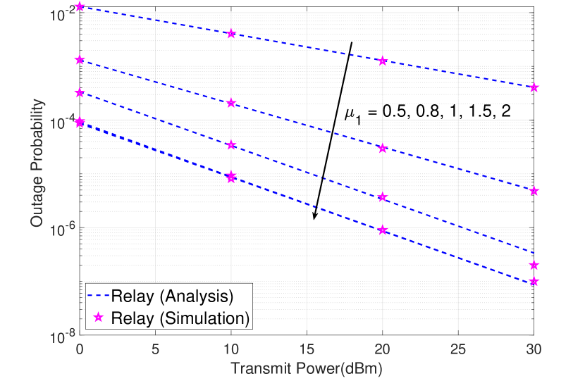
(a) Different values of $\mu_{1}$ at $\alpha_{1}=2,\alpha_{2}=2,\mu_{2}=1,\sigma_{s}=8{\rm cm},w_{z}/r_{1}=6,\gamma_{th}=4\mbox{dB}$, $\phi=28.9576$, and $S_{0}=0.054$.

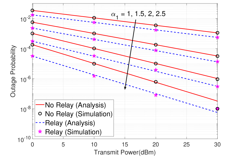
(b) Different values of $\alpha_{1}$ at $\mu_{1}=1,\alpha_{2}=2,\mu_{2}=4,\sigma_{s}=8{\rm{cm}},w_{z}/r_{1}=6,\gamma_{th}=4dB,\phi=28.9576$, and $S_{0}=0.054$.

Figure 2: Outage probability performance of relay-assisted THz-RF wireless link.

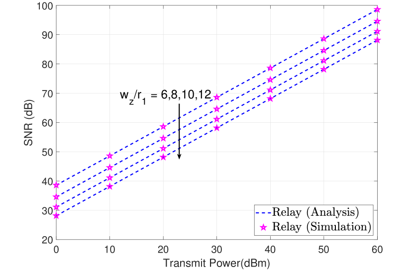
(a) Different values of $w_{z}/r_{1}$ at $\alpha_{1}=2,\mu_{1}=4,\alpha_{2}=2,\mu_{2}=1$, and $\sigma_{s}=15{\rm cm}$.

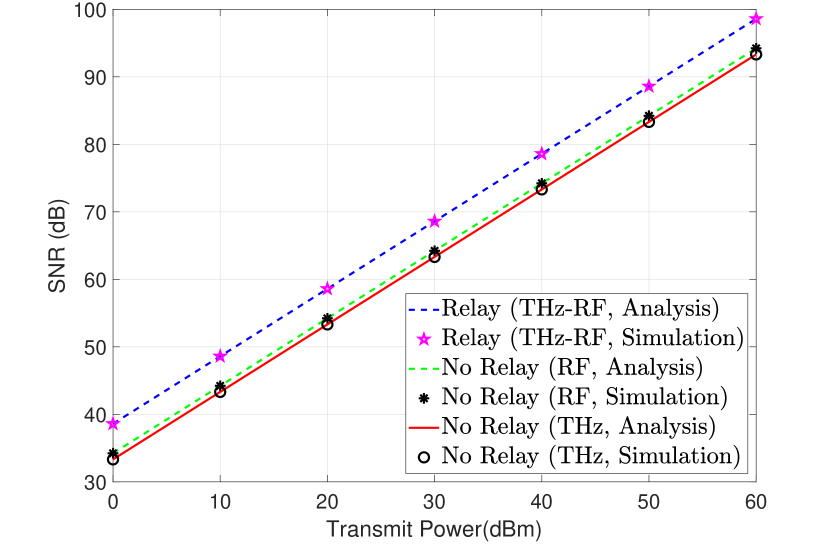
(b) Comparison between relayed and individual links at $\alpha_{1}=2,\mu_{1}=4,\alpha_{2}=2,\mu_{2}=1,\sigma_{s}=15{\rm cm},w_{z}/r_{1}=6,\phi=8.2368$, and $S_{0}=0.054$.

Figure 3: Average SNR performance of relay-assisted THz-RF wireless link.

First, we demonstrate the outage probability performance of the relay assisted system, as shown in Fig. 2. In Fig. 2a, we show the impact of the parameter $\mu$ on the outage probability by adopting the RF link as Rayleigh fading $\alpha_{2}=2$, $\mu_{2}=1$, and the THz link as the Nakagami-m fading $\alpha_{1}=2$ at different $\mu_{1}$. The outage performance improves with an increase in the parameter $\mu$ since an increase in $\mu_{1}$ accounts for dense clustering in the fading channel (i.e., good channel conditions). A very low value of $\mu_{1}<1$ (i.e., worse channel conditions, a typical scenario for the THz link) shows significant degradation in the outage performance. The derived CDF in Theorem 1 allows the computation of the outage probability for continuous (non-integer) values of $\mu_{1}$, which is necessary to evaluate the performance for a broader range of $\mu_{1}$, especially when $\mu_{1}<1$. It is noted that the state of art research use only integer values of $\mu_{1}$ to compute the CDF of the THz link [11]. Further, we show the effect of the non-linearity parameter $\alpha_{1}$ on the outage probability. In Fig. 2(b), we consider $\alpha_{2}=2$, $\mu_{2}=4$ (Nakagami-m fading with higher clustering) for the RF link and $\mu_{1}=2$ with different $\alpha_{1}$ of the THz link. The outage probability improves with an increase in the parameter $\alpha_{1}$ (i.e., a decrease in the non-linearity of the THz fading). The outage probability dramatically improves with an increase in the parameter $\alpha_{1}$: a factor of $10^{4}$ decrease in the outage probability when the parameter $\alpha_{1}$ increases from $1$ to $3$ at the same $10$ dBm of transmit power.

Observing Fig. 2a and Fig. 2b, it can be emphasized that the diversity order depends on $\alpha-\mu$ parameters of either of links since the parameter $\phi$ is higher (low pointing errors) due to strong normalized beam-width $w_{z}=0.6$. As such, analysis in (18)) shows that the diversity order $M=\mu_{1}$ depends on the THz link when $\mu_{1}<1$, and after that, there is no effect of the parameter $\mu_{1}$ since the diversity order becomes $M=1$, which is confirmed in Fig. 2a. Similar conclusions on the outage probability behavior on the parameter $\alpha_{1}$ can be inferred from Fig. 2b.

Next, we demonstrate the effect of pointing errors on the average SNR and ergodic rate performance of the relay-assisted system, as shown in Fig. 3 and Fig. 4. We consider Rayleigh fading ($\alpha_{2}=2$, $\mu_{2}=1$) for the RF and Nakamani-m fading ($\alpha_{1}=2$, $\mu_{1}=4$) for the THz link with standard deviation of jitter ($\sigma_{s}=15$ cm) and different values of normalized beam-width $\frac{w_{z}}{r_{1}}$. Fig. 3(a) and Fig. 4(a) demonstrate that the effect of pointing errors can be minimized by decreasing the normalized beam-width. It should be noted that the model of pointing errors in (4) is applicable when $w_{z}/r_{1}\geq 6$. In Fig. 3(b), we compare the performance of mixed THZ-RF transmissions with direct RF and THz. It can be seen that the relay-assisted system provides a significant (around $5$ dB) than the direct transmissions. There is a significant increase of $2$ bits/sec/Hz in the ergodic rate performance, as shown in Fig. 4(b). Although the direct link performance of THz and RF are almost similar, the THz has an enormous bandwidth (in the range of $10$ GHz) in comparison to the RF to get an enhanced channel capacity. It should be noted that the throughput of the THZ-RF system is limited by the bandwidth of RF link.

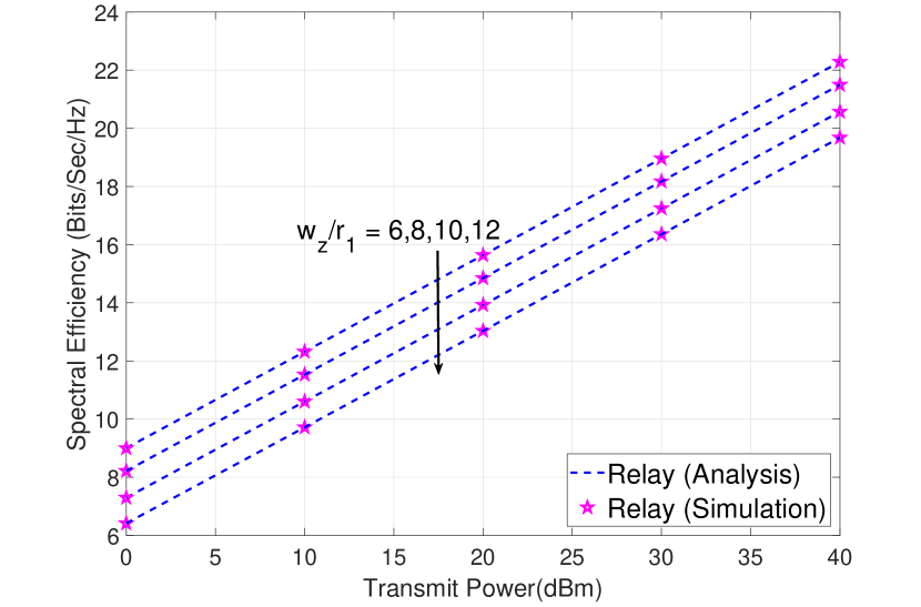
(a) Different values of $w_{z}/r_{1}$ at $\alpha_{1}=2,\mu_{1}=4,\alpha_{2}=2,\mu_{2}=1$, and $\sigma_{s}=15{\rm cm}$.

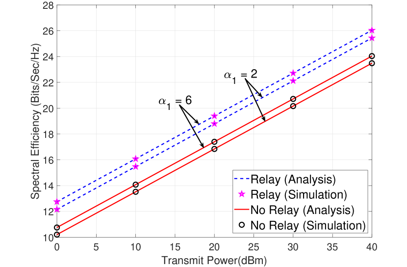
(b) Different values of $\alpha_{1}$, $\mu_{1}=1,\alpha_{2}=2,\mu_{2}=4,\sigma_{s}=15{\rm cm},w_{z}/r_{1}=6,\phi=8.2368$, and $S_{0}=0.054$.

Figure 4: Ergodic capacity performance of relay-assisted THz-RF wireless link.

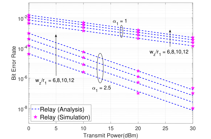
(a) Different values of $\alpha_{1}$ and $w_{z}/r_{1}$ at $\mu_{1}=1,\alpha_{2}=2,\mu_{2}=4$, and $\sigma_{s}=15{\rm cm}$.

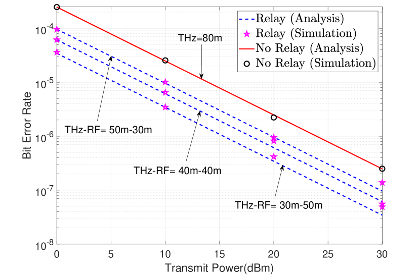
(b) Different link distances at $\alpha_{1}=2,\mu_{1}=1,\alpha_{2}=2,\mu_{2}=4,\sigma_{s}=15{\rm cm},w_{z}/r_{1}=6,\phi=8.2368$, and $S_{0}=0.054$.

Figure 5: Average BER performance of relay-assisted THz-RF wireless link.

Finally, we demonstrate the average BER performance in Fig. 5. We show the effect of fading parameter $\alpha_{1}$ and normalized beam-wdith $w_{z}/r_{1}$ on the average BER in Fig. 5(a). The figure shows a dramatic improvement in the average BER with an increase in $\alpha_{1}$ form $1$ to $2.5$. However, the effect of normalized beam-width $w_{z}/r_{1}$ on the average BER is nominal. In Fig. 5(b), we show the impact of relay location on the average BER performance for a link distance of $80$ m. It can be seen that a shorter THz link provides significant performance for the THz-RF relay system since the path loss at the THz frequencies is high.

In all the above plots (Fig. 2 to Fig. 5), we verified our derived expressions with the simulation and numerical results. It can be seen that the derived analytical expressions of the outage probability and average SNR for both i.i.d and i.ni.d fading scenarios and average BER for the i.i.d. fading have an exact match with the simulation results. The analytical results of ergodic capacity and average BER for the i.ni.d fading can overestimate/underestimate the exact results due to asymptotic bound $\Gamma(a,x)\to e^{-x}x^{a-1}$ in few terms of integration. However, Fig. 4 and Fig. 5 shows that the difference between analysis and simulation is indistinguishable. Further, the analytical results of ergodic capacity for the i.i.d fading are very close to the exact even with approximation $\log_{2}(1+x^{a})\approx a\log_{2}(1+x)$.

V Conclusions

We have investigated the performance of a THz-RF relay link over $\alpha$-$\mu$ fading with pointing errors. We considered a generalized i.ni.d. fading model by considering different $\alpha$ and $\mu$ parameters to model the short term fading for both the THz and RF links, along with the statistical distribution of pointing errors for the THz link. By deriving a closed-form expression of the CDF for the THz link, we analyzed the outage probability and diversity order of the system for real-valued $\mu$ and $\alpha$. The diversity order shows that the effect of pointing errors can be mitigated if the normalized beam width is adjusted sufficiently to get $\phi>\min\{\alpha_{1}\mu_{1},\alpha_{2}\mu_{2}\}$. We derived analytical expressions on average SNR, ergodic capacity, and average BER for a comprehensive analysis of the considered system. We also develop simplified expressions to provide insight on the system behavior analytically under various practically relevant scenarios. Simulation and numerical analysis show a significant effect of fading parameters $\alpha$ and $\mu$ of the THz link on the THz-RF system. However, compared with the fading parameters, the effect of normalized beam-width on the performance of relay-assisted is nominal. We have shown a significant gain in the performance of the relay-assisted system compared with the direct transmissions. The THz-RF link can achieve higher data rates, sufficient for data transmission between users and the central processing unit in a cell-free wireless network. The proposed work can be augmented by investigating the THz-RF system using the constant gain AF relaying by deriving the PDF of SNR $\gamma=\frac{\gamma_{1}\gamma_{2}}{\gamma_{2}+C}$, where $C$ is a constant.

Appendix A: Proof of Theorem 2

Using (9), we define $\bar{\gamma}_{1}^{(n)}=\int_{0}^{\infty}\gamma^{n}f_{1}(\gamma)d\gamma$, and substituting $\big{(}\sqrt{{\gamma}/{\gamma_{1}^{0}}}\big{)}^{\alpha_{1}}=t$, we get the $n$-th moment of SNR of the THz link

$$\bar{\gamma}_{1}^{(n)}=\frac{A_{1}{\gamma_{1}^{0}}^{n}}{\alpha_{1}}\int_{0}^{\infty}t^{(\frac{\phi-\alpha_{1}+2n}{\alpha_{1}})}\Gamma(B_{1},C_{1}t)dt$$ (55)

Using the identity [[54], 8.14.4] in (55), we solve the integral to get $\gamma_{1}^{(n)}$ of (25). Similarly, the $n$-th moment of SNR of the RF link is $\bar{\gamma}_{2}^{(n)}$=$\int_{0}^{\infty}\gamma^{n}f_{2}(\gamma)d\gamma$, which can be solved easily to get (25). Using (9) and (11) in $\bar{\gamma}_{12}^{(n)}=\int_{0}^{\infty}\gamma^{n}f_{1}(\gamma)\gamma F_{1}(\gamma)d\gamma$, and substituting $\big{(}\sqrt{{\gamma}/{\gamma_{1}^{0}}}\big{)}^{\alpha_{1}}=t$, we get

$$\bar{\gamma}_{12}^{(n)}=\frac{A_{1}{\gamma_{1}^{0}}^{n}}{\alpha_{1}}\bigg{[}\int_{0}^{\infty}t^{(\frac{\phi-\alpha_{1}+2n}{\alpha_{1}})}~{}\Gamma(B_{1},C_{1}t)~{}dt$$

$$- \frac{1}{\Gamma(\mu_{2})}\int_{0}^{\infty}t^{(\frac{\phi-\alpha_{1}+2n}{\alpha_{1}})}\Gamma(B_{1},C_{1}t){\Gamma\left(\mu_{2},B_{2}^{\prime}t^{\frac{\alpha_{2}}{\alpha_{1}}}\right)}dt\bigg{]}$$ (56)

where $B_{2}^{\prime}=B_{2}\sqrt{{\gamma_{1}^{0}}/{\gamma_{2}^{0}}}$. The first integral in (Appendix A: Proof of Theorem 2) is same as (55). To solve the second integral, we use the Meijer’s G representation of $\Gamma(B_{1},C_{1}t)$ and $\Gamma\big{(}\mu_{2},B_{2}^{\prime}t^{\frac{\alpha_{2}}{\alpha_{1}}}\big{)}$ to get the second integral as

$$I_{2}=\int_{0}^{\infty}t^{(\frac{\phi-\alpha_{1}+2n}{\alpha_{1}})}G_{1,2}^{2,0}\Big{(}\begin{matrix}1\\ B_{1},0\end{matrix}\Big{|}C_{1}t\Big{)}G_{1,2}^{2,0}\Big{(}\begin{matrix}1\\ \mu_{2},0\end{matrix}\Big{|}B_{2}^{\prime}t^{(\frac{\alpha_{2}}{\alpha_{1}})}\Big{)}dt$$ (57)

Using the identity [55] of definite integration of product of two Meijer’s G functions to get (22). Similarly, using (10) and (1) in $\bar{\gamma}_{21}^{(n)}=\int_{0}^{\infty}\gamma^{n}f_{2}(\gamma)\gamma F_{1}(\gamma)d\gamma$, and substituting $\big{(}\sqrt{{\gamma}/{\gamma_{2}^{0}}}\big{)}^{\alpha}=t$, we get

$$\bar{\gamma}_{21}^{(n)} =\frac{A_{1}A_{2}C_{1}^{-\frac{\phi}{\alpha_{1}}}{\gamma_{2}^{0}}^{n}}{\Gamma(\mu_{2})\phi}\bigg{[}\int_{0}^{\infty}t^{(\mu_{2}-1+\frac{2n}{\alpha_{2}})}e^{(-B_{2}t)}\Gamma(\mu_{1})dt$$

$$+\int_{0}^{\infty}t^{(\mu_{2}-1+\frac{2n}{\alpha_{2}})}e^{(-B_{2}t)}C_{1}^{\prime}t^{\frac{\phi}{\alpha_{2}}}\Gamma(B_{1},C_{1}^{\prime}t^{(\frac{\alpha_{1}}{\alpha_{2}})})dt$$

$$-\int_{0}^{\infty}t^{(\mu_{2}-1+\frac{2n}{\alpha_{2}})}e^{(-B_{2}t)}\Gamma(\mu_{1},C_{1}^{\prime}t^{(\frac{\alpha_{1}}{\alpha_{2}})})dt\bigg{]}$$ (58)

where $C_{1}^{\prime}=C_{1}\sqrt{{\gamma_{2}^{0}}/{\gamma_{1}^{0}}}$. The first integral in (Appendix A: Proof of Theorem 2) is similar to $\bar{\gamma}_{2}^{(n)}$ and can be similarly derived. To solve the second and third integrals, we use the identity [55] of definite integration of the product of two Meijer’s G functions to get (III-C).

Appendix B: Proof of lemma 1

Using (9), we define $\bar{\gamma}_{1}^{(n)}=\int_{0}^{\infty}\gamma^{n}f_{1}(\gamma)d\gamma$, and substituting $\big{(}\sqrt{{\gamma}/{\gamma_{1}^{0}}}\big{)}^{\alpha}=t$, we get the $n$-th moment of SNR of the THz link:

$$\bar{\gamma}_{1}^{(n)}=\frac{A_{1}{\gamma_{1}^{0}}^{n}}{\alpha}\int_{0}^{\infty}t^{(\frac{\phi-\alpha+2n}{\alpha})}\times\Gamma(B_{1},C_{1}t)dt$$ (59)

Using the identity [[54],8.14.4] in (59), we solve the integral to get $\gamma_{1}^{(n)}$ of (27). Similarly, the $n$-th moment of SNR of the RF link is $\bar{\gamma}_{2}^{(n)}=\int_{0}^{\infty}\gamma^{n}f_{2}(\gamma)d\gamma$, which can be solved easily to get (27). Using (9) and (11) in $\bar{\gamma}_{12}^{(n)}=\int_{0}^{\infty}\gamma^{n}f_{1}(\gamma)\gamma F_{1}(\gamma)d\gamma$, and substituting $\big{(}\sqrt{{\gamma}/{\gamma_{1}^{0}}}\big{)}^{\alpha}=t$, we get

$$\bar{\gamma}_{12}^{(n)} =\frac{A_{1}{\gamma_{1}^{0}}^{n}}{\alpha}\bigg{[}\int_{0}^{\infty}t^{(\frac{\phi-\alpha+2n}{\alpha})}\Gamma(B_{1},C_{1}t)dt$$

$$-\int_{0}^{\infty}t^{(\frac{\phi-\alpha+2n}{\alpha})}\Gamma(B_{1},C_{1}t)\left(\frac{\Gamma\left(\mu,B_{2}^{\prime}t\right)}{\Gamma(\mu)}\right)dt\bigg{]}$$ (60)

where $B_{2}^{\prime}=B_{2}\sqrt{{\gamma_{1}^{0}}/{\gamma_{2}^{0}}}$. The first integral in (Appendix B: Proof of lemma 1) is the same as (59). To solve the second integral, we apply the integration by parts tasking $\Gamma\left(\mu,B_{2}^{\prime}t\right)$ as the first term and $t^{(\frac{\phi-\alpha+2n}{\alpha})}\Gamma(B_{1},C_{1}t)$ as the second term, and use the identity [[49],eq.(6.455/1)] to get (1). Similarly, using (10) and (1) in $\bar{\gamma}_{21}^{(n)}=\int_{0}^{\infty}\gamma^{n}f_{2}(\gamma)\gamma F_{1}(\gamma)d\gamma$, and substituting $\big{(}\sqrt{{\gamma}/{\gamma_{2}^{0}}}\big{)}^{\alpha}=t$, we get

$$\bar{\gamma}_{21}^{(n)} =\frac{A_{1}A_{2}C_{1}^{-\frac{\phi}{\alpha}}{\gamma_{2}^{0}}^{n}}{\Gamma(\mu)\phi}\bigg{[}\int_{0}^{\infty}t^{(\mu-1+\frac{2n}{\alpha})}e^{(-B_{2}t)}\Gamma(\mu)dt$$

$$+\int_{0}^{\infty}t^{(\mu-1+\frac{2n}{\alpha})}e^{(-B_{2}t)}C_{1}^{\prime}t^{\frac{\phi}{\alpha}}\Gamma(B_{1},C_{1}^{\prime}t)dt$$

$$-\int_{0}^{\infty}t^{(\mu-1+\frac{2n}{\alpha})}e^{(-B_{2}t)}\Gamma(\mu,C_{1}^{\prime}t)dt\bigg{]}$$ (61)

where $C_{1}^{\prime}=C_{1}\sqrt{{\gamma_{2}^{0}}/{\gamma_{1}^{0}}}$. The first integral in (Appendix B: Proof of lemma 1) is similar to $\bar{\gamma}_{2}^{(n)}$ and can be similarly derived. For the second and third integrals, we use the identity [[49], eq.(6.455/1)] to get (1).

Appendix C: Proof of Theorem 3

Using (16) in (34), we represent the ergodic capacity of the relay assisted THz-RF link:

$$\bar{\eta}=\frac{1}{\Gamma(\mu_{2})\rm ln(2)}\int_{0}^{\infty}\frac{1}{1+\gamma}{\Gamma\left(\mu_{2},B_{2}{\gamma_{2}^{0}}^{\frac{-\alpha_{2}}{2}}\gamma^{\frac{\alpha_{2}}{2}}\right)}d\gamma$$

$$- \frac{A_{1}C_{1}^{-\frac{\phi}{\alpha_{1}}}}{\phi\Gamma(\mu_{2})\rm ln(2)}\bigg{[}\int_{0}^{\infty}\frac{1}{1+\gamma}\Gamma(\mu_{1}){\Gamma\left(\mu_{2},B_{2}{\gamma_{2}^{0}}^{\frac{-\alpha_{2}}{2}}\gamma^{\frac{\alpha_{2}}{2}}\right)}d\gamma$$

$$- \int_{0}^{\infty}\frac{\gamma^{\frac{\phi}{2}}}{1+\gamma}C_{1}{\gamma_{1}^{0}}^{\frac{-\phi}{2}}\Gamma\big{(}B_{1},C_{1}{\gamma_{1}^{0}}^{\frac{-\alpha_{1}}{2}}\gamma^{\frac{\alpha_{1}}{2}}\big{)}{\Gamma\left(\mu_{2},B_{2}{\gamma_{2}^{0}}^{\frac{-\alpha_{2}}{2}}\gamma^{\frac{\alpha_{2}}{2}}\right)}d\gamma$$

$$+ \int_{0}^{\infty}\frac{1}{1+\gamma}\Gamma\big{(}\mu_{1},C_{1}{\gamma_{1}^{0}}^{\frac{-\alpha_{1}}{2}}\gamma^{\frac{\alpha_{1}}{2}}\big{)}{\Gamma\left(\mu_{2},B_{2}{\gamma_{2}^{0}}^{\frac{-\alpha_{2}}{2}}\gamma^{\frac{\alpha_{2}}{2}}\right)}\bigg{]}d\gamma$$ (62)

We solve the first and second integral in (Appendix C: Proof of Theorem 3) exactly by applying the identity of definite integration of product of one power and one Meijer’s G function [56]. For the third integral, we use the series expansion of ${\Gamma\big{(}\mu_{2},B_{2}{\gamma_{2}^{0}}^{\frac{-\alpha_{2}}{2}}\gamma^{\frac{\alpha_{2}}{2}}\big{)}}$ using $\Gamma(a,bx)=(a-1)!\exp(-bx)\sum_{k=0}^{a-1}\frac{(bx)^{k}}{k!}$ and asymptotic expansion of $\Gamma\big{(}B_{1},C_{1}{\gamma_{1}^{0}}^{\frac{-\alpha_{1}}{2}}\gamma^{\frac{\alpha_{1}}{2}}\big{)}$ using $\Gamma(a,x)\approx e^{-x}x^{a-1}$. Employing $\alpha_{2}=\epsilon\alpha_{1}$, the third integral can be represented as

$$\bar{\eta}_{I_{3}}\approx \sum_{K_{2}=0}^{\mu_{2}-1}\frac{A_{1}C_{1}^{-\frac{\phi}{\alpha_{1}}+1}{\gamma_{1}^{0}}^{\frac{-\phi}{2}}(B_{2}{\gamma_{2}^{0}}^{-\frac{\alpha_{2}}{2}})^{k_{2}}(e^{-B_{2}{\gamma_{2}^{0}}^{-\frac{\alpha_{2}}{2}}})(C_{1}{\gamma_{1}^{0}}^{\frac{-\alpha_{1}}{2}})^{B_{1}-1}}{\phi\rm{ln(2)}k_{2}!}$$

$$\times \int_{0}^{\infty}{\gamma}^{\frac{\phi+K_{2}\alpha_{2}+B_{1}\alpha_{1}-3}{2}}e^{-\gamma^{\frac{\alpha_{1}}{2}}(C_{1}{\gamma_{1}^{0}}^{\frac{-\alpha_{1}}{2}}+\gamma^{\frac{\alpha_{1}(\epsilon-1)}{2}})}d\gamma$$ (63)

Thus, we apply the identity of definite integration of the product of one power and one Meijer’s G function [56] to solve $\bar{\eta}_{I_{3}}$ in (Appendix C: Proof of Theorem 3). For the fourth integral, we use the series expansion for gamma functions. Similar to the $\bar{\eta}_{I_{3}}$, we use $\alpha_{2}=\epsilon\alpha_{1}$ and apply the identity of definite integration of the product of one power and one Meijer’s G function [56] to solve the fourth integral. Capitalizing these, we get the ergodic capacity of THz-RF relay system in (III-D) of Theorem 3. It should be noted that the approximation is used in the last two terms that are not significant compared to the first two terms.

Appendix D: Proof of Lemma 2

Using (9) in (33), we define $\bar{\eta}_{1}\geq\int_{0}^{\infty}{\log}_{2}(\gamma)f_{1}(\gamma)d\gamma$, and substituting $\big{(}\sqrt{{\gamma}/{\gamma_{1}^{0}}}\big{)}^{\alpha}=t$, we get a lower bound average capacity of THz link:

$$\bar{\eta}_{1}\geq\frac{A_{1}}{\alpha\log(2)}\int_{0}^{\infty}{\rm log}(\gamma_{1}^{0}t^{\frac{2}{\alpha}})t^{(\frac{\phi}{\alpha}-1)}\Gamma(B_{1},C_{1}t)dt$$ (64)

It is noted that $\eta_{1}$ is a lower bound on the ergodic capacity of the THz link since $\log_{2}(1+\gamma)\geq\log_{2}(\gamma)$. To find a closed-form expression, we use integration by-parts with $\Gamma(B_{1},C_{1}t)$ as the first term and ${\rm log}(\gamma_{1}^{0}t^{\frac{2}{\alpha}})t^{(\frac{\phi}{\alpha}-1)}$ as the second term, and apply the identity [[49], (eq.4.352/1)] to get $\bar{\eta}_{1}$ in (1). Similarly, substituting $\big{(}\sqrt{{\gamma}/{\gamma_{2}^{0}}}\big{)}^{\alpha}=t$ in $\bar{\eta}_{2}\geq\int_{0}^{\infty}\rm{log}_{2}(\gamma)f_{2}(\gamma)d\gamma$ for a lower bound on the average capacity of the RF link:

$$\bar{\eta}_{2}\geq\frac{A_{2}}{\Gamma(\mu)\rm log(2)}\int_{0}^{\infty}{\log}(\gamma_{2}^{0}t^{\frac{2}{\alpha}})t^{(\mu-1)}e^{(-B_{2}t)}dt$$ (65)

We use the identity [[49], (eq.4.352/1)] in (65) to get $\bar{\eta}_{2}$ of (37). Defining $\bar{\eta}_{12}=\int_{0}^{\infty}{{\log}}_{2}(\gamma)f_{1}(\gamma)F_{2}(\gamma)d\gamma$, using (9) and (11), and substituting $\big{(}\sqrt{{\gamma}/{\gamma_{1}^{0}}}\big{)}^{\alpha}=t$, we get

$$\bar{\eta}_{12}\geq\frac{A_{1}}{\alpha\rm log(2)}\bigg{[}\int_{0}^{\infty}{\rm log}(\gamma_{1}^{0}t^{\frac{2}{\alpha}})t^{(\frac{\phi}{\alpha}-1)}\Gamma(B_{1},C_{1}t)dt$$

$$-\int_{0}^{\infty}{\rm log}(\gamma_{1}^{0}t^{\frac{2}{\alpha}})t^{(\frac{\phi}{\alpha}-1)}\Gamma(B_{1},C_{1}t)\left(\frac{\Gamma\left(\mu,B_{2}^{\prime}t\right)}{\Gamma(\mu)}\right)dt\bigg{]}$$ (66)

The first integral in (Appendix D: Proof of Lemma 2) is the same as (64). To solve the second integral, we use the series expansion of Gamma function $\Gamma(\mu,B_{2}^{\prime}t)=(\mu-1)!\exp(-B_{2}^{\prime}t)\sum_{k=0}^{\mu-1}\frac{(B_{2}^{\prime}t)^{k}}{k!}$. Using ${\rm log}(\gamma_{1}^{0}t^{\frac{2}{\alpha}})\approx\frac{2}{\alpha}{\rm log}(1+{\gamma_{1}^{0}}^{\frac{\alpha}{2}}t)$, and with Meijer’s G representation of ${\rm log}(1+{\gamma_{1}^{0}}^{\frac{\alpha}{2}}t)$, $\Gamma(B_{1},C_{1}t)$ and $\Gamma\left(\mu,B_{2}^{\prime}t\right)$, we get the second integral as

$$I_{2} \approx\sum_{k=0}^{\mu-1}\frac{2A_{1}(\mu-1)!B_{2}^{\prime k}}{\alpha^{2}\rm log(2)\Gamma(\mu)k!}\int_{0}^{\infty}t^{(\frac{\phi}{\alpha}+k-1)}G_{0,1}^{1,0}\Big{(}\begin{matrix}-\\ 0\end{matrix}\Big{|}B_{2}^{\prime}t\Big{)}$$

$$\times G_{1,2}^{2,0}\Big{(}\begin{matrix}1\\ B_{1},0\end{matrix}\Big{|}C_{1}t\Big{)}\Big{[}G_{2,2}^{1,2}\Big{(}\begin{matrix}1,1\\ 1,0\end{matrix}\Big{|}(\gamma_{1}^{0})^{\frac{\alpha}{2}}t\Big{)}\Big{]}dt$$ (67)

Finally, we apply the identity of definite integration of the product of three Meijer’s G function [57] to get $\bar{\eta}_{12}$ in (43). Similarly, using (10) and (1) we define $\bar{\eta}_{21}$ $\geq$ $\int_{0}^{\infty}{\log}_{2}(\gamma)f_{2}(\gamma)F_{1}(\gamma)d\gamma$ and substituting $\sqrt{{\gamma}/{\gamma_{2}^{0}}}^{\alpha}$=$t$, we get

$$\bar{\eta}_{21} \approx\frac{A_{1}C_{1}^{-\frac{\phi}{\alpha}}A_{2}}{\Gamma(\mu)\phi{\rm log(2)}}\bigg{[}\int_{0}^{\infty}{\rm log}(\gamma_{2}^{0}t^{\frac{2}{\alpha}})t^{(\mu-1)}e^{(-B_{2}t)}\Gamma(\mu)dt$$

$$+\int_{0}^{\infty}{\rm log}(\gamma_{2}^{0}t^{\frac{2}{\alpha}})t^{(\mu-1)}e^{(-B_{2}t)}C_{1}^{\prime}t^{\frac{\phi}{\alpha}}\Gamma(B_{1},C_{1}^{\prime}t)dt$$

$$-\int_{0}^{\infty}{\rm log}(\gamma_{2}^{0}t^{\frac{2}{\alpha}})t^{(\mu-1)}e^{(-B_{2}t)}\Gamma(\mu,C_{1}^{\prime}t)dt\bigg{]}$$ (68)

The first integral in (Appendix D: Proof of Lemma 2) is similar to $\eta_{2}$ of (65). To solve the second integral, we apply the identity of definite integration of the product of three Meijer’s G function [57]. Finally, to solve the third integration, we use the series expansion of Gamma function $\Gamma(\mu,C_{1}^{\prime}t)=(\mu-1)!\exp(-C_{1}^{\prime}t)\sum_{k=0}^{\mu-1}\frac{(C_{1}^{\prime}t)^{k}}{k!}$ and apply the identity of definite integration of the product of two Meijer’s G function [51]. Combining these three integrations, we get $\bar{\eta}_{21}$ in (2).

Appendix E: Proof of Theorem 4

Using (16) in (48), the average BER of the relay assisted THz-RF link can be expressed as

$$\bar{P}_{e}=\frac{A_{1}C_{1}^{-\frac{\phi}{\alpha_{1}}}q^{p}}{2\Gamma(p)\phi\Gamma(\mu_{2})}\Bigg{[}\int_{0}^{\infty}\gamma^{p-1}{e^{-q{\gamma}}}\Gamma(\mu_{1}){\Gamma\big{(}\mu_{2},B_{2}{\gamma_{2}^{0}}^{\frac{-\alpha_{2}}{2}}{\gamma}^{\frac{\alpha_{2}}{2}}\big{)}}d\gamma$$

$$+{C_{1}{\gamma_{1}^{0}}^{\frac{-\phi}{2}}}\int_{0}^{\infty}{\gamma}^{\frac{\phi+2p-2}{2}}{e^{-q{\gamma}}}\Gamma\Big{(}B_{1},C_{1}{\gamma_{1}^{0}}^{\frac{-\alpha_{1}}{2}}{\gamma}^{\frac{\alpha_{1}}{2}}\Big{)}{\Gamma\big{(}\mu_{2},B_{2}{\gamma_{2}^{0}}^{\frac{-\alpha_{2}}{2}}{\gamma}^{\frac{\alpha_{2}}{2}}\big{)}}d\gamma$$

$$-\int_{0}^{\infty}\gamma^{p-1}{e^{-q{\gamma}}}\Gamma\Big{(}\mu_{1},C_{1}{\gamma_{1}^{0}}^{\frac{-\alpha_{1}}{2}}{\gamma}^{\frac{\alpha_{1}}{2}}\Big{)}{\Gamma\big{(}\mu_{2},B_{2}{\gamma_{2}^{0}}^{\frac{-\alpha_{2}}{2}}{\gamma}^{\frac{\alpha_{2}}{2}}\big{)}}d\gamma\Bigg{]}$$

$$+\frac{q^{p}}{2\Gamma(p)}\int_{0}^{\infty}\gamma^{p-1}{e^{-q{\gamma}}}\bigg{(}1-\frac{\Gamma\big{(}\mu_{2},B_{2}{\gamma_{2}^{0}}^{\frac{-\alpha_{2}}{2}}{\gamma}^{\frac{\alpha_{2}}{2}}\big{)}}{\Gamma(\mu_{2})}\bigg{)}d\gamma$$ (69)

To solve the first integral in (Appendix E: Proof of Theorem 4), we apply the identity of definite integration of product of two Meijer’s G function [51]. For the second integral, we use the series expansion for ${\Gamma\big{(}\mu_{2},B_{2}{\gamma_{2}^{0}}^{\frac{-\alpha_{2}}{2}}\gamma^{\frac{\alpha_{2}}{2}}\big{)}}$ using $\Gamma(a,bx)$ =$(a-1)!e^{(-bx)}$ $\sum_{k=0}^{a-1}\frac{(bx)^{k}}{k!}$ and approximation for $\Gamma\big{(}B_{1},C_{1}{\gamma_{1}^{0}}^{\frac{-\alpha_{1}}{2}}\gamma^{\frac{\alpha_{1}}{2}}\big{)}$ using $\Gamma(a,x)\approx e^{-x}x^{a-1}$. Finally, using $\alpha_{2}=\epsilon\alpha_{1}$, the second integral becomes

$$\bar{P}_{eI_{2}}\approx\sum_{K_{2}=0}^{\mu_{2}-1}\frac{A_{1}C_{1}^{-\frac{\phi}{\alpha_{1}}+1}{\gamma_{1}^{0}}^{\frac{-\phi}{2}}(B_{2}{\gamma_{2}^{0}}^{-\frac{\alpha_{2}}{2}})^{k_{2}}(e^{-B_{2}{\gamma_{2}^{0}}^{-\frac{\alpha_{2}}{2}}})(C_{1}{\gamma_{1}^{0}}^{\frac{-\alpha_{1}}{2}})^{B_{1}-1}q^{p}}{2\Gamma(p)\phi k_{2}!}$$

$$\times\int_{0}^{\infty}{\gamma}^{\frac{\phi+K_{2}\alpha_{2}+\alpha_{1}(B_{1}-1)}{2}}e^{p-1}{e^{-q{\gamma}}}e^{-\gamma^{\frac{\alpha_{1}}{2}}(C_{1}{\gamma_{1}^{0}}^{\frac{-\alpha_{1}}{2}}+\gamma^{\frac{\alpha_{1}(\epsilon-1)}{2}})}d\gamma$$ (70)

Employing the identity of definite integration of the product of two Meijer’s G function [51], we solve the integral in (Appendix E: Proof of Theorem 4). For the third integral in (Appendix E: Proof of Theorem 4), we use the series expansion for gamma functions, and $\alpha_{2}=\epsilon\alpha_{1}$ to get an expression of the third integral. The fourth integral in (Appendix E: Proof of Theorem 4) can be solved applying the identity of definite integration of the product of two Meijer’s G function [51]. Capitalizing the expressions of these four integral, we get the average BER for the relay assisted link in (52) of Theorem 4.

References

• [1] P. Bhardwaj and S.M. Zafaruddin, “Performance of dual-hop relaying for THz-RF wireless link,” To be presented at 2021 IEEE 93rd Vehicular Technology Conference (VTC2021-Spring), Helsinki, Finland, 25-28 April 2021, preprint version: arXiv:2020.12186, 2020.
• [2] N. Bhushan, J. Li, D. Malladi, R. Gilmore, D. Brenner, A. Damnjanovic, R. T. Sukhavasi, C. Patel, and S. Geirhofer, “Network densification: the dominant theme for wireless evolution into 5G,” IEEE Communications Magazine, vol. 52, no. 2, pp. 82–89, 2014.
• [3] J. Liu, M. Sheng, L. Liu, and J. Li, “Network densification in 5G: From the short-range communications perspective,” IEEE Communications Magazine, vol. 55, no. 12, pp. 96–102, 2017.
• [4] A. Al-Dulaimi, S. Al-Rubaye, J. Cosmas, and A. Anpalagan, “Planning of ultra-dense wireless networks,” IEEE Network, vol. 31, no. 2, pp. 90–96, 2017.
• [5] S. Koenig, D.Lopez-Diaz, and J.Antes et al., “Wireless sub-THz communication system with high data rate,” Nature Photon, vol. 7, p. 977–981, 2013.
• [6] H. Elayan, O. Amin, B. Shihada, R. M. Shubair, and M. Alouini, “Terahertz band: The last piece of RF spectrum puzzle for communication systems,” IEEE Open Journal of the Communications Society, vol. 1, pp. 1–32, 2020.
• [7] A. Faisal, H. Sarieddeen, H. Dahrouj, T. Y. Al-Naffouri, and M. S. Alouini, “Ultramassive MIMO systems at Terahertz bands: Prospects and challenges,” IEEE Vehicular Technology Magazine, vol. 15, no. 4, pp. 33–42, 2020.
• [8] N. Wang, E. Hossain, and V. K. Bhargava, “Backhauling 5G small cells: A radio resource management perspective,” IEEE Wireless Communications, vol. 22, no. 5, pp. 41–49, 2015.
• [9] C. Wang, B. Lu, C. Lin, Q. Chen, L. Miao, X. Deng, and J. Zhang, “0.34-THz wireless link based on high-order modulation for future wireless local area network applications,” IEEE Transactions on Terahertz Science and Technology, vol. 4, no. 1, pp. 75–85, 2014.
• [10] A. A. Boulogeorgos and A. Alexiou, “Analytical performance assessment of THz wireless systems,” IEEE Access, vol. 7, pp. 11 436–11 453, 2019.
• [11] ——, “Error analysis of mixed THz-RF wireless systems,” IEEE Communications Letters, vol. 24, no. 2, pp. 277–281, 2020.
• [12] J. M. Jornet and I. F. Akyildiz, “Channel modeling and capacity analysis for electromagnetic wireless nanonetworks in the Terahertz band,” IEEE Transactions on Wireless Communications, vol. 10, no. 10, pp. 3211–3221, 2011.
• [13] S. Priebe, C. Jastrow, M. Jacob, T. Kleine-Ostmann, T. Schrader, and T. Kürner, “Channel and propagation measurements at 300 GHz,” IEEE Transactions on Antennas and Propagation, vol. 59, no. 5, pp. 1688–1698, 2011.
• [14] S. Kim and A. G. Zajić, “Statistical characterization of 300-GHz propagation on a desktop,” IEEE Transactions on Vehicular Technology, vol. 64, no. 8, pp. 3330–3338, 2015.
• [15] J. Kokkoniemi, J. Lehtomäki, and M. Juntti, “Simplified molecular absorption loss model for 275–400 Gigahertz frequency band,” in 12th European Conference on Antennas and Propagation (EuCAP 2018), 2018, pp. 1–5.
• [16] Y. Wu, J. Kokkoniemi, C. Han, and M. Juntti, “Interference and coverage analysis for Terahertz networks with indoor blockage effects and line-of-sight access point association,” IEEE Transactions on Wireless Communications, vol. 20, no. 3, pp. 1472–1486, 2021.
• [17] H. Sarieddeen, M. Alouini, and T. Y. Al-Naffouri, “Terahertz-band ultra-massive spatial modulation MIMO,” IEEE Journal on Selected Areas in Communications, vol. 37, no. 9, pp. 2040–2052, 2019.
• [18] C. Cheng, S. Sangodoyin, and A. Zajić, “Terahertz MIMO fading analysis and doppler modeling in a data center environment,” in 2020 14th European Conference on Antennas and Propagation (EuCAP), 2020, pp. 1–5.
• [19] A. Olutayo, J. Cheng, and J. F. Holzman, “A new statistical channel model for emerging wireless communication systems,” IEEE Open Journal of the Communications Society, vol. 1, pp. 916–926, 2020.
• [20] J. Bian, C. X. Wang, X. Gao, X. You, and M. Zhang, “A general 3D non-stationary wireless channel model for 5G and beyond,” IEEE Transactions on Wireless Communications, pp. 1–1, 2021.
• [21] P. Boronin, D. Moltchanov, and Y. Koucheryavy, “A molecular noise model for THz channels,” in 2015 IEEE International Conference on Communications (ICC), 2015, pp. 1286–1291.
• [22] V. Petrov, D. Moltchanov, and Y. Koucheryavy, “Interference and SINR in dense Terahertz networks,” in 2015 IEEE 82nd Vehicular Technology Conference (VTC2015-Fall), 2015, pp. 1–5.
• [23] R. Zhang, K. Yang, A. Alomainy, Q. H. Abbasi, K. Qaraqe, and R. M. Shubair, “Modelling of the Terahertz communication channel for in-vivo nano-networks in the presence of noise,” in 2016 16th Mediterranean Microwave Symposium (MMS), 2016, pp. 1–4.
• [24] H. Elayan, C. Stefanini, R. M. Shubair, and J. M. Jornet, “End-to-end noise model for intra-body Terahertz nanoscale communication,” IEEE Transactions on NanoBioscience, vol. 17, no. 4, pp. 464–473, 2018.
• [25] R. Boluda-Ruiz, A. García-Zambrana, C. Castillo-Vázquez, B. Castillo-Vázquez, and S. Hranilovic, “Outage performance of exponentiated Weibull FSO links under generalized pointing errors,” Journal of Lightwave Technology, vol. 35, no. 9, pp. 1605–1613, 2017.
• [26] J. Kokkoniemi, A. Boulogeorgos, M. Aminu, J. Lehtomäki, A. Alexiou, and M. Juntti, “Impact of beam misalignment on THz wireless systems,” Nano Communication Networks, vol. 24, p. 100302, 2020.
• [27] Z. Rong, M. S. Leeson, and M. D. Higgins, “Relay-assisted nanoscale communication in the THz band,” Micro Nano Letters, vol. 12, no. 6, pp. 373–376, 2017.
• [28] Q. H. Abbasi, A. A. Nasir, K. Yang, K. A. Qaraqe, and A. Alomainy, “Cooperative In-Vivo nano-network communication at Terahertz frequencies,” IEEE Access, vol. 5, pp. 8642–8647, 2017.
• [29] A. A. Boulogeorgos, E. N. Papasotiriou, and A. Alexiou, “Outage probability analysis of THz relaying systems,” arXiv:2007.07186, 2020.
• [30] T. Mir, M. Waqas, U. Mir, S. M. Hussain, A. M. Elbir, and S. Tu, “Hybrid precoding design for two-way relay-assisted Terahertz massive MIMO systems,” IEEE Access, vol. 8, pp. 222 660–222 671, 2020.
• [31] A. A. Farid and S. Hranilovic, “Outage capacity optimization for free-space optical links with pointing errors,” Journal of Lightwave Technology, vol. 25, no. 7, pp. 1702–1710, 2007.
• [32] M. D. Yacoub, “The $\alpha$-$\mu$ distribution: A physical fading model for the stacy distribution,” IEEE Transactions on Vehicular Technology, vol. 56, no. 1, pp. 27–34, 2007.
• [33] H. Du, J. Zhang, K. Guan, B. Ai, and T. Kürner, “Reconfigurable intelligent surface aided terahertz communications under misalignment and hardware impairments,” arXiv:2012.00267, 2020.
• [34] A. Nosratinia, T. E. Hunter, and A. Hedayat, “Cooperative communication in wireless networks,” IEEE Communications Magazine, vol. 42, no. 10, pp. 74–80, 2004.
• [35] Q. Li, R. Q. Hu, Y. Qian, and G. Wu, “Cooperative communications for wireless networks: techniques and applications in LTE-advanced systems,” IEEE Wireless Communications, vol. 19, no. 2, pp. 22–29, 2012.
• [36] E. Bjornson, M. Matthaiou, and M. Debbah, “A new look at dual-hop relaying: Performance limits with hardware impairments,” IEEE Transactions on Communications, vol. 61, no. 11, pp. 4512–4525, 2013.
• [37] E. Lee, J. Park, D. Han, and G. Yoon, “Performance analysis of the asymmetric dual-hop relay transmission with mixed RF/FSO links,” IEEE Photonics Technology Letters, vol. 23, no. 21, pp. 1642–1644, 2011.
• [38] I. S. Ansari, F. Yilmaz, and M. Alouini, “Impact of pointing errors on the performance of mixed RF/FSO dual-hop transmission systems,” IEEE Wireless Communications Letters, vol. 2, no. 3, pp. 351–354, 2013.
• [39] H. Samimi and M. Uysal, “End-to-end performance of mixed RF/FSO transmission systems,” IEEE/OSA Journal of Optical Communications and Networking, vol. 5, no. 11, pp. 1139–1144, 2013.
• [40] S. Anees and M. R. Bhatnagar, “Performance of an amplify and forward dual hop asymmetric RF FSO communication system,” IEEE/OSA Journal of Optical Communications and Networking, vol. 7, no. 2, pp. 124–135, February 2015.
• [41] L. Kong, W. Xu, L. Hanzo, H. Zhang, and C. Zhao, “Performance of a free-space-optical relay-assisted hybrid RF/FSO system in generalized $M$-distributed channels,” IEEE Photonics Journal, vol. 7, no. 5, pp. 1–19, Oct 2015.
• [42] E. Zedini, H. Soury, and M. Alouini, “On the performance analysis of dual-hop mixed FSO/RF systems,” IEEE Transactions on Wireless Communications, vol. 15, no. 5, pp. 3679–3689, May 2016.
• [43] B. Bag, A. Das, I. S. Ansari, A. Prokeš, C. Bose, and A. Chandra, “Performance analysis of hybrid FSO systems using FSO/RF-FSO link adaptation,” IEEE Photonics Journal, vol. 10, no. 3, pp. 1–17, 2018.
• [44] Y. Zhang, J. Zhang, L. Yang, B. Ai, and M. Alouini, “On the performance of dual-hop systems over mixed FSO/mmWave fading channels,” IEEE Open Journal of the Communications Society, vol. 1, pp. 477–489, 2020.
• [45] A. A. Boulogeorgos, E. N. Papasotiriou, J. Kokkoniemi, J. Lehtomaeki, A. Alexiou, and M. Juntti, “Performance evaluation of THz wireless systems operating in 275-400 GHz band,” in 2018 IEEE 87th Vehicular Technology Conference (VTC Spring), 2018, pp. 1–5.
• [46] A. Papoulis and S. Pillai, Probability, Random Variables, and Stochastic Processes.   McGraw Hill, Boston, Fourth Edition, 2002.
• [47] G. J. O. Jameson, “The incomplete gamma functions,” The Mathematical Gazette, vol. 100, Iss. 548, pp. 298–306, Jul 2016.
• [48] A. Annamalai, R. C. Palat, and J. Matyjas, “Estimating ergodic capacity of cooperative analog relaying under different adaptive source transmission techniques,” in 2010 IEEE Sarnoff Symposium, 2010, pp. 1–5.
• [49] I. S. Gradshteyn and I. M. Ryzhik , Table of Integrals, Series, and Products.   Academic press, San Diego, CA, 6th edition, 2000.
• [50] I. S. Ansari, S. Al-Ahmadi, F. Yilmaz, M. Alouini, and H. Yanikomeroglu, “A new formula for the BER of binary modulations with dual-branch selection over generalized-k composite fading channels,” IEEE Transactions on Communications, vol. 59, no. 10, pp. 2654–2658, 2011.
• [51] The Wolfram function Site, Accessed: Sept. 26, 2020. Available: http://functions.wolfram.com/HypergeometricFunctions/MeijerG/21/02/03/01.
• [52] C. Balanis, Antenna Theory: Analysis and Design.   John Wiley and Sons, 3rd Edition, 2016.
• [53] P.  Sen, D. A. Pados, S. N. Batalama, E. Einarsson, J. P. Bird, and J. M. Jornet, “The TeraNova platform: An integrated testbed for ultra-broadband wireless communications at true Terahertz frequencies,” Computer Networks, Elsevier, 2020.
• [54] Incomplete Gamma and Realted Functions, Accessed: Sept. 26, 2020 [Online]. Available: http://dlmf.nist.gov/8.14.
• [55] V. Adamchik and O. Marichev, The algorithm for calculating integrals of hypergeometric type functions and its realization in reduce system.   John Wiley and Sons, 3rd Edition, 1990.
• [56] The Wolfram function Site, Accessed: Jan. 08, 2021. Available: https://functions.wolfram.com/HypergeometricFunctions/MeijerG/21/02/07/.
• [57] The Wolfram function Site, Accessed: Sept. 26, 2020. Available: http://functions.wolfram.com/07.34.21.0012.01.