Abstract

Global value chains (GVCs) are formed through value-added trade, and some regions promote economic integration by concluding regional trade agreements to promote these chains. However, there is no way to quantitatively assess the scope and extent of economic integration involving various sectors in multiple countries. In this study, we used the World Input–Output Database to create a cross-border sector-wise trade in value-added network (international value-added network (IVAN)) covering the period of 2000–2014 and evaluated them using network science methods. By applying Infomap to the IVAN, we confirmed for the first time the existence of two regional communities: Europe and the Pacific Rim. Helmholtz–Hodge decomposition was used to decompose the value flows within the region into potential and circular flows, and the annual evolution of the potential and circular relationships between countries and sectors was clarified. The circular flow component of the decomposition was used to define an economic integration index, and findings confirmed that the degree of economic integration in Europe declined sharply after the economic crisis in 2009 to a level lower than that in the Pacific Rim. The European economic integration index recovered in 2011 but again fell below that of the Pacific Rim in 2013. Moreover, sectoral analysis showed that the economic integration index captured the effect of Russian mineral resources, free movement of labor in Europe, and international division of labor in the Pacific Rim, especially in GVCs for the manufacture of motor vehicles and high-tech products.

Introduction

It is difficult to grow a country’s economy without establishing economic relations with other countries. Every year, the amount of international trade increases along with the world’s GDP. Free trade agreements (FTAs) and regional trade agreements (RTAs) have been created to support this trend, and countries are working to stabilize trade.

How, then, do countries become interdependent through trade? Classically, Ricard advocated comparative advantage, which stated that countries specializing in different industries are supposed to trade by taking advantage of their respective strengths. However, in recent years, trade in intermediate goods, which did not exist at that time, has begun and flourished. In other words, there are forms of trade specializing in different industries and GVCs in the same industry to produce complex and sophisticated products. In addition, distance (as represented by the gravity model) and economic integration (such as that promoted by the EU and NAFTA) facilitate international trade.

Many studies have been conducted on measuring international production structures. In the 21st century, measurement of GVCs became a widely discussed topic after Hummels et al. [1] proposed the vertical specialization index. Moreover, the VAX and FVAiX indices were proposed by Johnson and Noguera [2] and Amador et al. [3], respectively. Koopman et al. [4] decomposed and classified the trade prices into nine terms and clarified double-counted terms.

The abovementioned progress has led to the development of international input–output (IO) tables. After the World Input–Output Database (WIOD) was publicized by Dietzenbacher et al. [5] and Timmer et al. [6] [7], Cerina et al. [8] and Zhu et al. [9] analyzed the data for measuring GVCs network analysis methods. Los et al. [10] showed that GVCs have been fragmenting more rapidly than regionally in 1995–2011. According to Johnson and Noguera [11], over a period of 40 years, the ratio of value-added to gross exports in non-manufacturing sectors rose, while that in manufacturing sectors fell by 20 percentage points; their study showed that RTAs led to such decline.

Due to international relationship problems in the economy, researchers in international organizations have been analyzing GVCs. Recently comprehensive summary reports of GVC research have been published by the World Bank [12] [13]. According to these reports, GVC research aims to address misunderstanding of trade data and give international trade opportunities and export diversity to developing countries for economic growth [14]. As shown by Degain et al., GVCs had been expanding until the global financial crisis, but it stopped growing in 2011 when it recovered from a decline in equipment. The GVC expansion seen before the financial crisis has been interpreted as China’s accession to the WTO and participation in GVCs [14]. These GVC research developments were described in detail by Amador and Cabral [15] and Inomata [16]. However, economics studies mainly focus on the relationship between nations. There are limited works showing the complicated relationship between industries in different countries.

By contrast, there are many studies on international trade in network science because of recent developments in analytical methods and data availability. Initially, the scale-free characteristics of international trade networks were clarified [17][18][19]; then, the virtual nodes in these networks were examined using centrality indices and other measures, and changes over time were analyzed [20][21][22].

Ikeda et al. [23] [24] studied the international trade network of the WIOD using community analysis of modularity maximization, which combines the synchronization aspect of the G7 production network [25] [26]; then, they found stable sectoral communities that had emerged in 1995–2011.

From an institutional point of view, a study examining interregional agreements and geographic factors in international trade change found no evidence that the WTO has contributed to the increase in international trade and indicated that geographic factors are more significant than interregional agreements [27]. By contrast, other studies show that trade policies contribute to shaping trade networks [28], and the impact of distance by trade is decreasing in industrial sectors [29].

However, there is no way to quantitatively assess the scope and extent of economic integration involving various sectors in multiple countries. It is difficult to quantitatively evaluate such economic phenomena, where multiple countries and sectors are intertwined, and the trade balance between two countries is still used as a basis for foreign economic policy. In this study, we analyze the economic linkages through trade that have been made in recent years using international IO tables and network science methods and clarify how the world economy is being integrated from the perspective of value-added trade.

In this context, this study offers the following essential contributions. First, rather than using trade figures, which can mislead international economic relations, we used the value-added calculations used in an IO analysis to construct a sector-wise network. Next, from the value-added linkage, we confirmed the regional characteristics of Europe and the Pacific Rim. Findings showed that the behavior of this value-added relationship is highly different from that of the sectoral community in the international trade network shown in previous studies. The dense economic relationships within these regions were decomposed into potential and circular relationships, and the countries and sectors that contribute to the strong regional ties were identified. Finally, we propose an economic integration index that is based on the circular flow component, and the results showed that economic integration was higher in the Pacific Rim than in Europe in 2010, 2013, and 2014.

The remainder of this paper is organized into three parts. The next section describes the IO table and the computational method used in this work to create the network and the community analysis, explains the decomposition of the potential and circular flow components, and presents the proposed method for measuring economic integration. Then, the characteristics and structure of the network, the potential and circular relationships, and the results of the integration index are presented, and the international economic linkages are examined on the basis of these results. Finally, we conclude this study.

Data and methods

This section consists of four subsections. First, we describe the WIOD and the computational methods used to build the cross-border, sector-wise trade in value-adde network (IVAN). Second, we briefly describe Infomap, a community analysis algorithm, which was used to determine the extent to which economic integration is occurring. Third, we explain the use of Helmholtz–Hodge decomposition to extract the potential and circular nature of IVANs. Finally, the economic integration index is defined.

Data

We used the WIOD released in 2016, which includes 43 countries and classifies the rest of the world (RoW) into 56 sectors. These countries and sectors are listed in S1 Table. and S2 Table: List of sectors.. The country codes are the same as those of the WIOD, but we simplified the sectoral codes. The WIOD has IO tables for 2000–2014. Table 1 shows a simplified example of the table. The IO table was developed by Leontief [30] and is now used globally to estimate economic and environmental conditions. In this paper, we used the WIOD without RoW because we aim to analyze the relationships of specific countries.

Table 1: World input–output table with two sectors in three countries.

		Intermediate demand						Final demand
		Country A		Country B		Country C					Total output
		Sector 1	Sector 2	Sector 1	Sector 2	Sector 1	Sector 2	Country A	Country B	Country C
Country A	Sector 1	$Z_{1,1}$	$Z_{1,2}$	$Z_{1,3}$	$Z_{1,4}$	$Z_{1,5}$	$Z_{1,6}$	$FD_{1,1}$	$FD_{1,2}$	$FD_{1,3}$	$T_{1}$
	Sector 2	$Z_{2,1}$	$Z_{2,2}$	$Z_{2,3}$	$Z_{2,4}$	$Z_{2,5}$	$Z_{2,6}$	$FD_{2,1}$	$FD_{2,2}$	$FD_{2,3}$	$T_{2}$
Country B	Sector 1	$Z_{3,1}$	$Z_{3,2}$	$Z_{3,3}$	$Z_{3,4}$	$Z_{3,5}$	$Z_{3,6}$	$FD_{3,1}$	$FD_{3,2}$	$FD_{3,3}$	$T_{3}$
	Sector 2	$Z_{4,1}$	$Z_{4,2}$	$Z_{4,3}$	$Z_{4,4}$	$Z_{4,5}$	$Z_{4,6}$	$FD_{4,1}$	$FD_{4,2}$	$FD_{4,3}$	$T_{4}$
Country C	Sector 1	$Z_{5,1}$	$Z_{5,2}$	$Z_{5,3}$	$Z_{5,4}$	$Z_{5,5}$	$Z_{5,6}$	$FD_{5,1}$	$FD_{5,2}$	$FD_{5,3}$	$T_{5}$
	Sector 2	$Z_{6,1}$	$Z_{6,2}$	$Z_{6,3}$	$Z_{6,4}$	$Z_{6,5}$	$Z_{6,6}$	$FD_{6,1}$	$FD_{6,2}$	$FD_{6,3}$	$T_{6}$
Value-added		$VA_{1}$	$VA_{2}$	$VA_{3}$	$VA_{4}$	$VA_{5}$	$VA_{6}$
Total output		$T_{1}$	$T_{2}$	$T_{3}$	$T_{4}$	$T_{5}$	$T_{6}$

Calculation for adjacency matrix of IVAN

Let $n_{c}$ be the number of countries and $n_{s}$ be the number of sectors in the IO table. Then, we define the $n_{c}n_{s}\times n_{c}n_{s}$ intermediate matrix $\mathbf{Z}$, $n_{c}n_{s}\times n_{c}$ final demand matrix $\mathbf{FD}$, $1\times n_{c}n_{s}$ value-added vector $\mathbf{VA}$, and $1\times n_{c}n_{s}$ total output matrix $\mathbf{T}$. With use of the value-added vector $\mathbf{VA}$ and total output vector $\mathbf{T}$, the value-added coefficient vector $\mathbf{V}$ is calculated as $\mathbf{VA}/(\mathbf{T})^{\top}$. Therefore, an induced value-added vector $\hat{\mathbf{V}}\mathbf{L}\mathbf{F}$ is made by a vector $\mathbf{L}\mathbf{F}$ left-hand multiplied by the $n_{c}n_{s}\times n_{c}n_{s}$ diagonal matrix $\hat{\mathbf{V}}$, where the diagonal components are the vector $\mathbf{V}$.

Then, the adjacency matrix of the global value-added network (GVAN) $\mathbf{G}$ is calculated as $\hat{\mathbf{V}}\mathbf{L}\hat{\mathbf{F}}$, where $\hat{\mathbf{F}}$ is a diagonal matrix whose diagonal components are the vector $\mathbf{F}$. The IVAN’s adjacency matrix $\mathbf{Y}$ was created by eliminating components of 43 on-diagonal $56\times 56$ blocks as zero from $\mathbf{G}$. This matrix represents the sum of all the ripple effects of value-added induced by the final demand in foreign sectors. The GVAN and IVAN nodes comprise 56 sectors in 43 countries. S1 Table. and S2 Table: List of sectors. list these countries and sectors.

In summary, IVANs are directed and weighted networks constructed by the adjacency matrix $Y$, which does not have domestic links. By contrast, GVANs have domestic and international links.

Community detection

To know how each network develop a community structure, we apply community analysis to IVANs. Some community analysis methods have been developed, and their features were summarized by Fortunato and Hric [33] and Barabási [34]. We used Infomap, which is an application of random walk and Huffman coding [35] to analyze the communities in the studied network [36]. Let a random walker run in the network where this analysis will be applied; the random walker transitions with a probability dependent on the path weights (plus a constant transposition probability) [37]. The map equation establishes communities and renames the node in which the random walk track’s code length is minimized. In comparison, the well-known method of modularity maximization clusters a network by counting nodes’ link weights, inflows, and outflows, whereas the map equation method clusters a network by the remaining time of the random walker in the nodes; this difference leads to variations in results [36] [32].

In the Infomap method, the optimization problem for community segmentation in a network is replaced with the minimization problem of the code length of a segmented network. Consider the segmentation of a network composed of $n$ nodes into $m$ communities with a community partition $\mathsf{M}$. Let the mean code length of segmented communities (index code length) be $H(\mathcal{Q})$ and the mean code length of nodes within a community $i$ be $H(\mathcal{P}^{i})$; then, with use of Shannon’s source coding theorem [38], the average description length of a single step of the random walk $L(M)$ is calculated as follows:

$$L(\mathsf{M})=q_{\curvearrowright}H(\mathcal{Q})+\sum_{i=1}^{m}p_{\circlearrowright}^{i}H(\mathcal{P}^{i}),$$ (1)

where $q_{\curvearrowright}$ is the probability of the random walker moving to another community and $p_{\circlearrowright}^{i}$ is the probability of the random walker moveing within a community $i=1,2,\ldots,m$ plus the exit probability from $i$. Each of the probabilities is defined as $q_{\curvearrowright}=\sum_{i=1}^{m}q_{i\curvearrowright}$ and $p_{\circlearrowright}^{i}=\sum_{\alpha\in i}p_{\alpha}+q_{i\curvearrowright}$, where $p_{\alpha}$ is the probability of visiting node $\alpha=1,2,\ldots,n$ and $q_{i\curvearrowright}$ is the exit probability from community $i$. Eq (1) is called the map equation [32].

Structural characteristics of networks

Certain indices reveal network characteristics. We used eleven indices: (1) density, reciprocity, diameter, average path length, average betweenness, assortativity, average in-degree, and average out-degree are calculated as unweighted and directed networks; (2) in-strength and out-strength are for weighted and directed ones; (3) the clustering coefficient is calculated as unweighted and undirected [34].

The density of a network is the proportion of the number of links to the number of maximum possible links in the network. Thus, it is calculated as $l/n(n-1)$, where $n$ and $l$ are the numbers of nodes and links in the network, respectively.

The reciprocity of a network is the proportion of the reciprocal links to the total number of links in the network. It is calculated as $l_{m}/l$, where $l_{m}$ is the number of reciprocal links (two directed links between two nodes in the network).

The clustering coefficient indicates how each node is connected to its neighbors. The clustering coefficient $c_{i}$ of a node $i$ is calculated as $c_{i}=l_{i}/k_{i}(k_{i}-1)$, where $l_{i}$ ($k_{i}$) is the number of links (neighbors) of node $i$. Thus, the clustering coefficient of a network is $\sum c_{i}/n$.

The diameter of a network is the maximum number of shortest paths for all pairs of nodes in the network.

The average path length of a network is the mean of the shortest path length in the network: $\sum_{i,j;i\neq j}d_{ij}/n(n-1)$, where $d_{ij}$ is the shortest path length between nodes $i$ and $j$.

The betweenness is calculated by the number of the shortest paths through a node. The betweenness $b_{i}$ of node $i$ is $\sum_{j\neq k\neq i}s_{jk}(i)/s_{jk}$, where $s_{jk}$ is the number of the shortest paths between nodes $j$ and $k$, and $s_{jk}(i)$ is the number of the shortest paths through node $i$. Therefore, the average betweenness of a network is the mean of $b_{i}$.

The degree of a node means the sum of the number of links in the node. There are two kinds of degrees in a directed network, namely, in-degree and out-degree, which are the sums of the links to the node from the other nodes (inflow) and links from the node to other nodes (outflow), respectively. Thus, the in-degree and out-degree are represented as: $\sum_{j}l_{j,i}$ and $\sum_{j}l_{i,j}$, respectively, where $l_{i,j}$ is a link (flow) from node $i$ to node $j$.

The assortativity of a network scores the similarity of the connections in the network as -1 to 1, which is calculated by $(\sum_{jk}jke_{jk}-\mu)/\sigma^{2}$, where $e_{jk}$ is the probability of the two nodes of degrees $j$ and $k$ are at the end of a randomly chosen link, and $\mu$ and $\sigma$ are the mean and standard deviation, respectively, of the excess degree distribution. Assortativity that is close to -1 (1) indicates that high-degree nodes in a network are connected to low-degree nodes (high-degree nodes).

The strength of a node is the total weight of the links in the node. There are two kinds of strength, in a directed network, namely, in-strength and out-strength, which are the summed weights of the inflow and outflow, respectively. Thus, the in-strength and out-strength are represented as: $\sum_{j}l^{w}_{j,i}$ and $\sum_{j}l^{w}_{i,j}$, respectively, where $l^{w}_{i,j}$ is the flow amount from node $i$ to node $j$.

Decomposition to potential and circular flows

Firstly, we define flows as directed and weighted links, and the flow of IVANs as value flow. We used Helmholtz–Hodge decomposition [39] to extract potential and circular relationships from IVANs. This method was also used by Kichikawa et al. [40] to clarify the potential relationships in corporate transaction networks. With Helmholtz–Hodge decomposition, the flow $F_{ij}$ from node $i$ to node $j$ can be separated into the circular flow $F_{ij}^{(c)}$ and potential flow $F_{ij}^{(p)}$: $F_{ij}=F_{ij}^{(c)}+F_{ij}^{(g)}$. Here the potential flow $F^{(p)}_{ij}$ is given by $F^{(p)}_{ij}=w_{ij}(\phi_{i}-\phi_{j})$, where $\phi_{i}$ is the Helmholtz–Hodge potential and $w_{ij}$ is a positive weight for the link between node $i$ and node $j$. The circular flow satisfies $\sum_{j}F^{(c)}_{ij}=0$, in which the inflows and outflows are balanced in each node. $F_{ij}^{(p)}$ represents the difference in potentials between the nodes, whereas $F_{ij}^{(c)}$ represents the number of feedback loops among the nodes.

An IVAN captures the value-added chain of various international sectors to their respective final goods. The potential of a sector is the difference between the amount of value adde by the sector for final foreign production and the amount of value added by the foreign sector for the sector’s final production. In other words, if the value-added potential is positive, the sector contributes more to the production of the final goods of the foreign sector, and if it is negative, the sector is contributed more to the own production of the final goods by foreign sectors. This can indicate the degree of asymmetric dependence or co-dependence. Moreover, the circular flow component indicates the amount of contribution to (from) the foreign sector, that is, the degree of interdependence.

Economic integration index

When several economies proceed with economic integration by some factors such as the establishment of FTAs or RTAs, the value added in a country becomes increasingly induced by other countries, and vice versa. In other words, higher economic integration makes a larger feedback loop within an IVAN. On the basis of this assumption, we define the economic integration index $E$ as the aggregate amount of circular flow divided by the total flow of the GVAN in a specific community.

$$E=\frac{\sum_{i>j}Y_{ij}^{(c)}}{\sum G_{ij}}$$ (2)

The range of application of this index covers communities detected by Infomap, which also detects communities using flow. The detected communities are interpreted as the circulation observed when random walkers rotate in the community. The degree of circulation is quantified and divided by the economic scale of the community; then, the economic integration is measured as the amount of value-added circulation per economic scale.

The index defined here indicates how much of the domestic and international value-added chain toward final demand can be extracted as international interdependence. The higher the value of the index, the greater the value-added induced in the community across national borders (economic activities performed by sectors in other countries), and economic integration in this study is measured by this value.

This economic integration index can decompose into sectoral indices arbitrarily. For sector $k$, the sectoral economic integration index is

$$E_{k}=\frac{\sum_{i>j;i,j\in S_{k}}Y_{ij}^{(c)}}{\sum_{i,j\in S_{k}}G_{ij}},$$ (3)

where $S_{k}$ is a set of nodes in sector $k$.

In summary, the economic integration index is the circular magnitude of the cross-border value-added contribution of economic activities in a country (other countries) toward the final production of sectors in other countries (home country), compared with the circular magnitude of the value-added contribution of economic activities in the community, including circulation within a country.

Results

This section is composed of three subsections. The first subsection shows the community structure of the IVANs, the threshold set for community detection, and the resulting 15-year change in regional communities. The second subsection shows the basic characteristics of the original IVAN, the cut IVAN, and the IVAN of the regional communities in selected years. The third subsection confirms the value-added potential and circular relationships revealed by Helmholtz–Hodge decomposition for countries and sectors in Europe and the Pacific Rim. The last subsection shows the evolution of economic integration in the regional communities and the results of decomposing the economic integration indicators into key sectoral components.

Communities of IVANs

Direct application of Infomap to the IVANs reveals one large community for 15 years. This result differs from the community of international trade network shown in a previous study. Next, thresholds are set to exclude the branches and leaves of the IVANs to see any concealed community structure. In the range of 6,500–11,000 remaining links, several large communities appear (Fig 1). Here, the thresholds are set by the number of the most extensive links to be retained, as the threshold value set by USD is inappropriate for the weight of the IVAN links, which fluctuates due to the economic growth and economic crisis that occurred in those 15 years. In Fig 1, each cell colored on the number of communities with more than 240 nodes which is 10% of the total nodes in the IVANs. The remaining number of links in 2014 is almost half of that in 2004–2009.

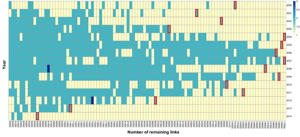
Fig 1: Heat map of the number of large communities in the IVANs cut by each threshold, in 2000–2014. This research uses the thresholds represented as a red cell in each year. Colors means the number of communities.

By using the abovementioned threshold values, we can detect the communities from the IVANs as shown in Fig 2 which shows four years’ heat maps and represents each cell as a node of the IVANs. In the maps, the separated communities are indicated by different colors; the gray cells are the nodes that were not considered communities. The figure shows orange horizontal stripes, which include most of the sectors in countries such as Australia, Brazil, and Canada. The green nodes include the sectors A01: agriculture, C29: manufacture of motor vehicles, and C30: manufacture of other transport equipment of mainly European countries. The gray area includes many other sectors in Europe, especially in small countries.

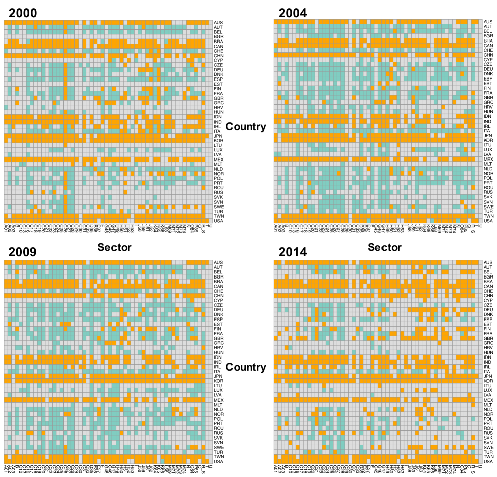
Fig 2: Community heat maps in 2000, 2004, 2009, and 2014. Each cell is a node of IVAN, the gray nodes are not a communities, while the other colors indicate community. The green and orange cells are nodes of the European and Pacific Rim communities, respectively. The regional classification is in S1 Table..

The results of community detection 15 years are shown in Fig 3 as a Sankey diagram, where orange represents the Pacific Rim sectors, and the green represents the European sectors (nodes) (the details of the classification are in S1 Table.), and we can see that these two regions are detected as separate communities throughout the 15 years.

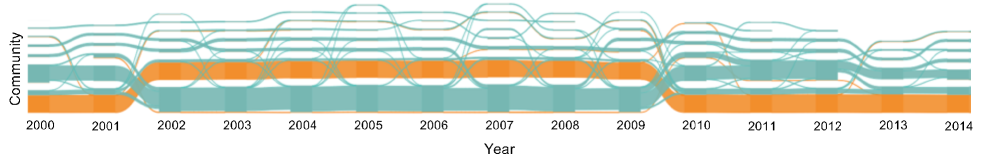
Fig 3: Sankey diagram of communities in 2000–2014. Communities are ordered by size, from the largest to the smallest, each year. Green and orange represent nodes of Europe and the Pacific Rim, respectively. Their classification of them is in S1 Table.. The two bottom communities are used to denote regional communities, but there have been other small European communities over the years.

Observed structural characteristics

Table 2 shows the structural features for 2000, 2008, and 2014. The densities and cluster coefficients show that the IVANs are dense, and the reciprocity shows that more than 97% of the links are mutual. The density of the IVANs that are cut at the threshold in Fig. 1 is reduced by about 82%. In terms of reciprocities, the cut IVANs are about 20% of the remaining links that are cut. This indicates that the IVAN have many asymmetric mutualities with large values in only one direction. In the two local communities, the cluster coefficients and reciprocities are at the same level as those of the IVANs, although the densities are about 10% higher than those of the entire IVANs.

Table 2: Structural characteristics of IVANs, IVANs cut with the threshold, IVANs in the regional communities: Europe and the Pacific Rim.

	2000				2008				2014
	IVAN	Cut IVAN	Europe	Pacific Rim	IVAN	Cut IVAN	Europe	Pacific Rim	IVAN	Cut IVAN	Europe	Pacific Rim
Density	0.831	0.0174	0.942	0.921	0.841	0.0184	0.955	0.925	0.831	0.0112	0.945	0.929
Reciprocity	0.972	0.231	0.987	0.976	0.982	0.192	0.990	0.987	0.974	0.169	0.993	0.975
Clustering coefficient	0.976	0.321	0.953	0.941	0.976	0.319	0.963	0.934	0.976	0.278	0.950	0.950
Diameter	2	5	2	2	2	4	2	2	2	6	2	2
Average path length	1.023	2.474	1.046	1.056	1.023	2.55	1.035	1.063	1.023	2.656	1.048	1.048
Average betweenness*	51.70	2644	24.62	37.14	51.72	3053	28.99	37.37	51.64	2835	14.32	35.82
Assortativity	-0.0167	-0.436	-0.0394	-0.0304	-0.0179	-0.427	-0.0294	-0.0305	-0.0170	-0.424	-0.0505	-0.0304
Average in-degree*	2196	71.68	516.4	622	2198	71	788	556.8	2193	52.59	281.7	715.3
Average out-degree*	2143	68.71	509.7	610.7	2164	65.5	780.3	553	2147	45.61	279.8	703

*These averages were calculated for nonzero values.

Each IVAN has a diameter of 2, which means that any sector in any country can be connected to all sectors through one sector in another country. The minimum diameter is 2 because links to sectors in the same country are not included, but since the average path length is close to 1, most sectors are directly connected. In the cut IVANs, the diameter is about 5, and the average betweenness is more than 50 times larger than that of the original IVANs because the diameter and average path length are long, and a particular node mediates many shortest paths. In the regional communities, the average path length is a slightly longer, and the betweenness is roughly half of the original IVANs.

The number of nodes in the IVANs is 2,408, but the average in-degree and out-degree value is over 2,100. Since most of the sectors are connected, the assortativity is close to zero. In the cut IVANs, the degrees and assortativity are around 70 and -0.43, respectively, indicating that sectors with degree differences are connected by high values flows. In the regional communities, the degree varies according to the size of the detected regional community, and the assortativity is negative, close to zero.

Fig 4 shows a wide strength distribution of the IVAN’s. The distribution of Fig 4 partly fits a log-normal distribution, especially in the right tail. The probability density function of a log-normal distribution $p(x)$ for $x>0$ is:

$$p(x)=\frac{1}{\sqrt{2\pi}\sigma x}\exp\biggl{[}-\frac{(\log x-\mu)^{2}}{2\sigma^{2}}\biggr{]},$$ (4)

where $\mu$ and $\sigma$ are the mean and standard deviation of the logarithm, respectively. As seen in Fig 4, the mean and standard deviation of the logarithm of strength distribution in 2014 are $\mu=5.959$ and $\sigma=2.129$ in in-strength, and $\mu=6.146$ and $\sigma=2.001$ in out-strength, respectively.

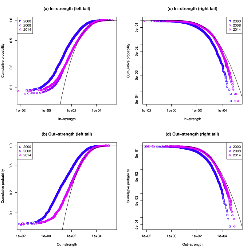
Fig 4: Cumulative probability of strength of IVAN in 2000, 2008, and 2014. The black lines are plots of the cumulative density function of the log-normal distribution whose $\mu$ and $\sigma$ are equal to the average and the standard deviation, respectively, of the logarithm of strength distribution in 2014. Their right tails are almost fitted, but the left tails are not, especially at the bottom.

Potential and circular relationships in two regional communities

Helmholtz–Hodge decomposition was applied to the two regional communities detected by Infomap. The size of the circular flow component and the value of the IVAN link (value flow) are well correlated in the range where the value flow is greater than 100 million USD, as shown in Fig 5. In the economic integration index, the amount of circular flow is divided by the GVAN weights; thus, the economic scale does not appear directly.

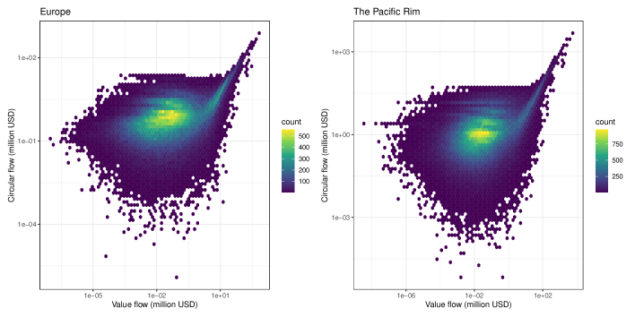
Fig 5: Scatter plot of correlation between circular flow and value flow in 2000. The larger circular flows are in proportion to the original value flows, but the lower flows are disarranged.

The potential and circular relationships in Europe and the Pacific Rim can be analyzed from the international and intersectoral perspectives by aggregating nodes into countries and sectors.

Europe

Tables 2–7 show the breakdown of the potential and circular relationships in Europe, which is obtained from the Helmholtz–Hodge decomposition. In terms of countries, the value potential is mainly high in Russia, Norway, and Germany and low in France, Spain, and Italy (Table 3). From 2003 to 2012, Russia and Norway mainly have the first and second highest potential, respectively. In 2001, 2002, and 2010, with changes in the ranking of the communities in Fig 3, Germany shows the highest potential. In 2000 and 2001, 2010, and since 2013, when the European community was relatively small (Fig 3), Russia had not been in Table 3. In addition, Belgium, Switzerland, and the Netherlands repeatedly appear in Table 3. Non-European countries, such as the United States, are ranked fourth from 2002 to 2005, while China is fourth in 2009 and 2010. France is ranked the lowest-potential country except in 2002 and 2003, when Spain is ranked first, followed by Italy (Table 4). Portugal and Turkey are also ranked in half of the years. Tables 3 and 4 show that Germany is ranked as both a high-potential and low-potential country.

Table 3: Five highest-potential countries in Europe.

Rank	2000	2001	2002	2003	2004	2005	2006	2007	2008	2009	2010	2011	2012	2013	2014
1	NLD	DEU	DEU	RUS	RUS	RUS	RUS	RUS	RUS	RUS	DEU	RUS	RUS	POL	DEU
2	DEU	BEL	RUS	NOR	NOR	NOR	NOR	NOR	NOR	NOR	GBR	NOR	NOR	ITA	RUS
3	CHE	CHE	NOR	DEU	DEU	DEU	DEU	DEU	NLD	DEU	BEL	NLD	NLD	CZE	NLD
4	BEL	NLD	USA	USA	USA	USA	NLD	NLD	CHE	CHN	CHN	IRL	DNK	AUT	GBR
5	NOR	FIN	NLD	NLD	BEL	BEL	USA	BEL	AUT	BEL	AUT	CYP	USA	NLD	HUN

Table 4: Five lowest-potential countries in Europe.

Rank	2000	2001	2002	2003	2004	2005	2006	2007	2008	2009	2010	2011	2012	2013	2014
1	FRA	FRA	ESP	ESP	FRA	FRA	FRA	ESP	FRA	FRA	FRA	FRA	FRA	FRA	FRA
2	ESP	ESP	ITA	FRA	ESP	ESP	ESP	FRA	ESP	ITA	ITA	DEU	DEU	BEL	CHE
3	ITA	DNK	FRA	ITA	ITA	ITA	ITA	GBR	DEU	ESP	ESP	ITA	GBR	GBR	DNK
4	PRT	PRT	POL	POL	HUN	TUR	TUR	TUR	TUR	GBR	LUX	GBR	TUR	RUS	ESP
5	DNK	POL	PRT	HUN	POL	HUN	POL	ITA	POL	LUX	DNK	POL	POL	DEU	TUR

Russia is ranked first in the high-potential tables (Tables 3 and 5) except for 2002, when sector B: mining and quarrying is ranked first. If the sector B: mining and quarrying was not considered in Table 5 and Russia were not included in Table 3. The other highest-potential sectors in Europe are M69: legal, accounting, and consultancy activities in 2000 and 2010; C24: manufacture of basic metals in 2001; C25: manufacture of fabricated metal products, except machinery and equipment in 2013; and G46: wholesale trade except that of motor vehicles and motorcycles in 2014. In addition, sectors N: administrative and support service activities and C20: manufacture of chemicals and chemical products are often ranked high. In terms of low potential (Tables 4 and 6), sector F: construction is ranked first throughout the 15 years, followed by sectors C28: manufacture of machinery and equipment, C19: manufacture of coke and refined petroleum products, C29: manufacture of motor vehicles, which occupy the second and subsequent positions; O84: public administration and defense, and compulsory social security, which appears in the third and subsequent positions; and L68: real estate activities, which often appears in the fifth position.

Table 5: Five highest-potential sectors in Europe.

Rank	2000	2001	2002	2003	2004	2005	2006	2007	2008	2009	2010	2011	2012	2013	2014
1	M69	C24	B	B	B	B	B	B	B	B	M69	B	B	C25	G46
2	C24	N	N	N	N	N	N	C24	C24	M69	G46	G46	G46	C24	C24
3	N	M69	M69	M69	M69	C24	C24	N	G46	N	N	N	N	C22	C25
4	C20	C20	C24	C24	C24	M69	M69	G46	M69	G46	C24	C24	M69	G46	C20
5	K64	C25	C20	C20	C20	G46	G46	M69	H49	C24	C20	H49	C24	C27	C22

B: mining and quarrying; C20: manufacture of chemicals and chemical products; C22: manufacture of rubber and plastic products; C24: manufacture of basic metals; C25: manufacture of fabricated metal products except machinery and equipment; C27: manufacture of electrical equipment; G46: wholesale trade except trade of motor vehicles and motorcycles; H49: land transport and transport via pipelines; K64: financial service activities except insurance and pension funding; M69: legal and accounting activities; activities of head offices, and management consultancy activities; N: administrative and support service activities.

Table 6: Five lowest-potential sectors in Europe.

Rank	2000	2001	2002	2003	2004	2005	2006	2007	2008	2009	2010	2011	2012	2013	2014
1	F	F	F	F	F	F	F	F	F	F	F	F	F	F	F
2	C28	C28	C28	C28	C19	C19	C19	C29	C29	C19	C28	C19	C19	C29	C28
3	C19	O84	O84	O84	C28	C28	C28	C19	C19	C28	O84	C28	C28	C28	O84
4	O84	C31	C19	C19	O84	O84	O84	C28	C28	O84	G47	D35	D35	O84	G47
5	C31	L68	L68	L68	L68	R_S	R_S	O84	O84	L68	C31	O84	O84	R_S	C33

C19: manufacture of coke and refined petroleum products; C28: manufacture of machinery and equipment n.e.c.; C29: manufacture of motor vehicles, and trailers, and semi-trailers; C31: manufacture of furniture, and other manufacturing; C33: repair and installation of machinery and equipment; D35: electricity, gas, steam and air conditioning supply; F: construction; G47: retail trade except that of motor vehicles and motorcycles; L68: real estate activities; O84: public administration and defense, and compulsory social security; R_S: other service activities.

According to the amount of circulation (Table 7), Germany is the top country for the 15 years, followed by France, the United Kingdom, Italy, and Russia. In terms of sectoral ranking (Table 8), sector F: construction is always ranked first until 2010. In 2011 and 2012, sector B: mining and quarrying, which often ranks second, is ranked first. In 2013, sector C29: manufacture of motor vehicle is first. Russia is ranked second in the year that sector B: mining and quarrying is ranked first. Throughout the whole years, F: construction is first, followed by B: mining and quarrying, C28: manufacture of machinery and equipment, C19: manufacture of coke and refined petroleum products, and G46: wholesale trade except for that of motor vehicles and motorcycles.

Table 7: Five-highest circulated countries in Europe.

Rank	2000	2001	2002	2003	2004	2005	2006	2007	2008	2009	2010	2011	2012	2013	2014
1	DEU	DEU	DEU	DEU	DEU	DEU	DEU	DEU	DEU	DEU	DEU	DEU	DEU	DEU	DEU
2	FRA	FRA	GBR	FRA	FRA	FRA	FRA	FRA	RUS	FRA	FRA	RUS	RUS	FRA	FRA
3	NLD	ITA	FRA	ITA	GBR	GBR	GBR	ITA	FRA	RUS	ITA	NOR	GBR	ITA	ITA
4	ITA	ESP	ITA	GBR	ITA	ITA	RUS	RUS	ITA	GBR	ESP	FRA	NOR	ESP	POL
5	ESP	GBR	ESP	ESP	NLD	RUS	ITA	GBR	NOR	ITA	NLD	GBR	FRA	POL	AUT

Table 8: Five-highest circulated sectors in Europe.

Rank	2000	2001	2002	2003	2004	2005	2006	2007	2008	2009	2010	2011	2012	2013	2014
1	F	F	F	F	F	F	F	F	B	F	F	B	B	C29	F
2	C28	C28	B	B	B	B	B	B	F	B	C28	F	F	F	C28
3	G46	G46	N	N	C19	C19	C19	C29	C19	C19	G46	C19	C19	C28	G46
4	K64	C20	G46	G46	N	G46	G46	C19	C29	G46	M69	G46	D35	C25	C25
5	C20	C24	C28	C28	G46	C28	C28	G46	G46	D35	K64	D35	G46	C24	C20

B: mining and quarrying; C19: manufacture of coke and refined petroleum products; C20: manufacture of chemicals and chemical products; C24: manufacture of basic metals; C25: manufacture of fabricated metal products, except machinery and equipment; C28: manufacture of machinery and equipment n.e.c.; C29: manufacture of motor vehicles, and trailers and semi-trailers; D35: electricity, gas, steam and air conditioning supply; F: construction; G46: wholesale trade except that of motor vehicles and motorcycles; K64: financial service activities except insurance and pension funding; M69: legal and accounting activities, activities of head offices, and management consultancy activities; N: administrative and support service activities.

For both countries and sectors, those ranked higher or lower in terms of potential are also greater in terms of circular strength, which is the strength of the circular network decomposed from an IVAN. The relationship between the circular strength and the Helmholtz–Hodge potential is shown in Fig 6. The relationship is V-shaped; in other words, the larger the absolute value of the potential, the higher the circular strength.

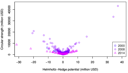
Fig 6: Scatter plot of correlation between circular strength and Helmholtz–Hodge potential in Europe in 2000, 2008, and 2014. Each year shows a V-shaped pattern, but the inclination is changed (sharpest in 2008 and gentlest in 2014).

Pacific Rim

The characteristics of the potential and circular flows of the IVANs in the Pacific Rim are shown in Tables 8–13. Japan, which has the maximum potential in 2000 and 2002, has been out of the ranking since 2012; Canada shows the maximum potential from 2003 to 2007, and Australia has been the highest-potential country since then (Table 9). Indonesia, Taiwan, and India are also among the five highest-potential countries. In terms of low potential, Mexico is the top-ranked country until 2002, the United States from 2004 to 2006, and China in 2003 and from 2007 to 2013. In addition, India, the United Kingdom, and France appear in Table 10 numerous times.

Table 9: Five highest-potential countries in the Pacific Rim.

Rank	2000	2001	2002	2003	2004	2005	2006	2007	2008	2009	2010	2011	2012	2013	2014
1	JPN	CAN	JPN	CAN	CAN	CAN	CAN	CAN	AUS	AUS	AUS	AUS	AUS	AUS	AUS
2	CAN	JPN	CAN	JPN	JPN	JPN	AUS	AUS	CAN	CAN	JPN	CAN	CAN	CAN	CAN
3	AUS	AUS	AUS	AUS	AUS	AUS	JPN	JPN	IDN	JPN	CAN	IDN	IDN	TWN	TWN
4	IDN	IDN	TWN	IDN	IDN	IDN	IDN	TWN	TWN	TWN	IDN	JPN	TWN	RUS	KOR
5	TWN	TWN	IDN	TWN	KOR	TWN	TWN	IDN	BRA	IDN	TWN	TWN	BRA	IDN	DEU

Table 10: Five lowest-potential countries in the Pacific Rim.

Rank	2000	2001	2002	2003	2004	2005	2006	2007	2008	2009	2010	2011	2012	2013	2014
1	MEX	MEX	MEX	CHN	USA	USA	USA	CHN	CHN	CHN	CHN	CHN	CHN	CHN	USA
2	CHN	CHN	USA	USA	CHN	CHN	CHN	USA	USA	MEX	MEX	IND	USA	USA	CHN
3	USA	GBR	CHN	MEX	MEX	MEX	MEX	MEX	MEX	IND	GBR	MEX	IND	MEX	MEX
4	GBR	IND	IND	IND	GBR	IRL	IRL	IND	KOR	GBR	IND	KOR	MEX	IDN	IND
5	IND	USA	FRA	FRA	IND	IND	GBR	HUN	HUN	DEU	KOR	USA	FRA	GBR	GBR

In terms of sectoral potential (Tables 11 and 12), as in Europe, B: mining and quarrying is the highest-potential sector, and F: construction is the lowest-potential sector. The relationship is more stable than that in Europe and remains unchanged over the 15 years. In addition, as shown in Table 11, sectors B: mining and quarrying, C20: manufacture of chemicals and chemical products, C24: manufacture of basic metals, G46: wholesale trade, K64: financial service activities, and N: administrative and support service activities are included in the high-potential sectors. Sectors F: construction; O84: public administration and defense, and compulsory social security; C29: manufacture of motor vehicles; C10: manufacture of food products, beverages, and tobacco products; and Q: human health and social work activities are among the lowest-potential sectors until 2009 except 2001. Since 2010, Q: human health and social work activities have risen to higher than third place.

Table 11: Five highest-potential sectors in the Pacific Rim.

Rank	2000	2001	2002	2003	2004	2005	2006	2007	2008	2009	2010	2011	2012	2013	2014
1	B	B	B	B	B	B	B	B	B	B	B	B	B	B	B
2	C20	C20	C20	C20	C20	C24	C24	C24	C24	C24	C20	C24	C24	G46	G46
3	C24	C24	C24	C24	C24	C20	C20	G46	G46	C20	G46	C20	G46	C24	C24
4	G46	G46	G46	G46	G46	G46	G46	C20	C20	G46	C24	G46	C20	C20	C20
5	N	N	C25	K64	K64	K64	K64	K64	K64	K64	N	N	K64	K64	K64

B: mining and quarrying; C20: manufacture of chemicals and chemical products; C24: manufacture of basic metals; C25: manufacture of fabricated metal products except machinery and equipment; G46: wholesale trade except that of motor vehicles and motorcycles; K64: financial service activities except insurance and pension funding; N: administrative and support service activities.

Table 12: Five lowest-potential sectors in the Pacific Rim.

Rank	2000	2001	2002	2003	2004	2005	2006	2007	2008	2009	2010	2011	2012	2013	2014
1	F	F	F	F	F	F	F	F	F	F	F	F	F	F	F
2	O84	O84	O84	O84	O84	O84	O84	O84	O84	O84	O84	O84	O84	Q	O84
3	C29	C29	C29	C29	C29	C29	C29	C29	C29	C29	Q	Q	Q	O84	Q
4	C10	Q	C10	C10	C10	C10	C10	C10	C10	C10	C29	C29	C29	C29	C29
5	Q	C10	Q	Q	Q	Q	Q	Q	Q	Q	C10	C10	C10	C10	C10

C10: manufacture of food products, beverages and tobacco products; C29: manufacture of motor vehicles, and trailers and semi-trailers; F: construction; O84: public administration and defense, and compulsory social security; Q: human health and social work activities.

In terms of circulation (Tables 13 and 14), the United States is consistently in the first place, followed by Japan, Canada, and China since 2007. Since 2005, Japan has been in the fourth place, followed by Mexico. By contrast, the sector rankings in Table 14 are not as consistent as those of the countries. In 2000 and 2007, C26: manufacture of computer, electronic, and optical products is ranked first; in 2008 and 2011, B: mining and quarrying is ranked first. These three sectors remain in the top three positions over the 15 years. They are followed by C29: manufacture of motor vehicles and O84: public administration and defense, and compulsory social security until 2009, and by O84: public administration and defense, and compulsory social security and Q: human health and social work activities since 2010.

Table 13: Five highest-circulated countries in the Pacific Rim.

Rank	2000	2001	2002	2003	2004	2005	2006	2007	2008	2009	2010	2011	2012	2013	2014
1	USA	USA	USA	USA	USA	USA	USA	USA	USA	USA	USA	USA	USA	USA	USA
2	JPN	CAN	CAN	CAN	CAN	CAN	CAN	CHN	CHN	CHN	CHN	CHN	CHN	CHN	CHN
3	CAN	JPN	JPN	JPN	JPN	CHN	CHN	CAN	CAN	CAN	CAN	CAN	CAN	CAN	CAN
4	MEX	MEX	MEX	CHN	CHN	JPN	JPN	JPN	JPN	JPN	JPN	JPN	JPN	JPN	JPN
5	CHN	CHN	CHN	MEX	MEX	MEX	MEX	MEX	MEX	MEX	MEX	MEX	MEX	MEX	MEX

Table 14: Five highest-circulated sectors in the Pacific Rim.

Rank	2000	2001	2002	2003	2004	2005	2006	2007	2008	2009	2010	2011	2012	2013	2014
1	C26	F	F	F	F	F	F	C26	B	F	F	B	B	F	F
2	F	C26	C26	C26	B	B	B	F	C26	B	B	F	F	B	B
3	B	B	B	B	C26	C26	C26	B	F	C26	C26	C26	C26	C26	C26
4	C29	O84	C29	O84	O84	C29	O84	O84	O84	O84	O84	O84	O84	O84	O84
5	O84	C29	O84	C29	C29	O84	C29	C29	C29	C29	C29	Q	Q	Q	Q

B: mining and quarrying; C26: manufacture of computer, electronic, and optical products; C29: manufacture of motor vehicles, and trailers and semi-trailers; F: construction; O84: public administration and defense, and compulsory social security; Q: human health and social work activities.

As in Europe, the high- or low-potential countries and sectors in the Pacific Rim are high in circular strength. The relationship between the circular strength and the Helmholtz–Hodge potential is shown in Fig 7. The V-shaped relationship between them is the same as that in Europe. However, there is a difference in the tables 2–14. Sector C26: manufacture of computer, electronic, and optical products does not appear in Tables 11 and 12, which indicates a large value-added circulation in the midstream of the Pacific Rim’s value flow, although all high-circular-strength sectors in Europe are also in the value-added potential ranking.

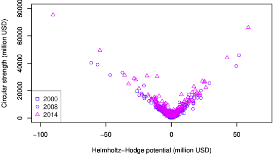
Fig 7: Scatter plot of correlation between circular strength and Helmholtz-Hodge potential in the Pacific Rim in 2000, 2008, and 2014. The years show the similar inclinations of the V shape.

Economic integration index

The results of applying the economic integration index to the two regional communities are shown in Fig 8. The Pacific Rim shows a stable and upward trend for economic integration, while Europe shows a higher but more unstable integration level. In particular, there is a large decline in the level of integration in 2009 and 2010, after the economic crisis, while the Pacific Rim is slightly affected in 2009.

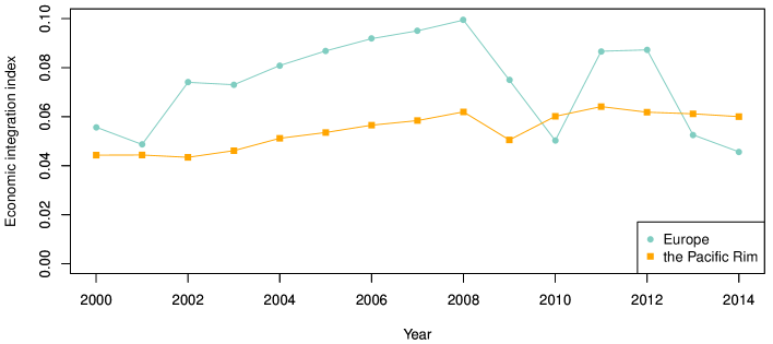
Fig 8: Economic integration estimation of the two regional communities in 2000–2014.

Figs 9, 10, and 11 show the sector-wise economic integration indices, focusing on the sectors that show high circulation in Tables 8 and 14. As illustrated in Fig 9, Europe exhibits a fivefold increase in 2007 and 2008 (just before the economic crisis) in sector B: mining and quarrying and F: construction (the top-ranking sectors in terms of potential and circular flows) compared with 2000, then a sharp decline from 2009 to 2010 (below 2000 level). The low values in 2010, 2013, and 2014 are partly due to a decline in F: construction, but the circulation within B: mining and quarrying is almost zero. By contrast, in the Pacific Rim, these values are tripled between 2007 and 2008; they decline beginning 2011, but they remain above 2007 levels in 2014.

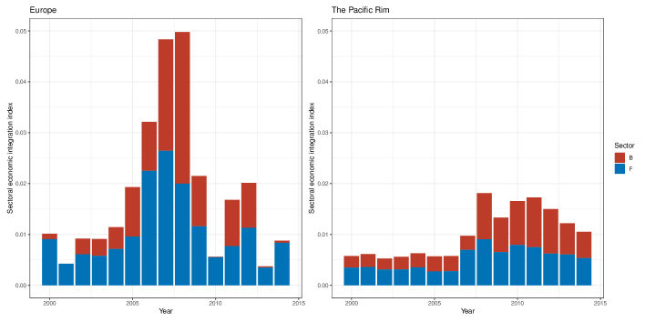
Fig 9: Sectoral economic integration index of mining and quarrying, and construction. B: mining and quarrying, F: construction.

Fig 10 shows the sectoral economic integration indices of the manufacturing sectors ranked in Tables 8 and 14. The figure illustrates that the increase in the amount of circulation in the manufacturing sectors plays a major role in Europe having the largest economic integration index in 2008. Sector C29: manufacture of motor vehicles makes a significant contribution in 2007 and 2008. Sectors C24: manufacture of basic metals, C25: manufacture of fabricated metal products, and C29: manufacture of motor vehicles exhibit the highest values in 2008. The high value in 2008 can be seen from the fact that C24: manufacture of basic metals, C25: manufacture of fabricated metal products, and C29: manufacture of motor vehicles show the highest values throughout the 15 years. As for the manufacturing sectors, C19: manufacture of coke and refined petroleum products disappears from the European community at a time when the economic integration index for B: mining and quarrying is nearly zero. On the contrary, in the Pacific Rim, the manufacturing sector steadily increases its contribution to economic integration. In the years with large values in economic integration index, C19: manufacture of coke and refined petroleum products, C20: manufacture of chemicals and chemical products, and C29: manufacture of motor vehicles are large in sectoral indices.

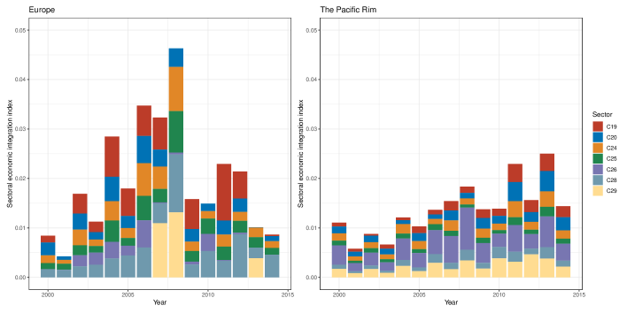
Fig 10: Sectoral economic integration index of manufacture. C19: manufacture of coke and refined petroleum products; C20: manufacture of chemicals and chemical products; C24: manufacture of basic metals, C25: manufacture of fabricated metal products except machinery and equipment; C26: manufacture of computer, electronic, and optical products; C28: manufacture of machinery and equipment n.e.c.; C29: manufacture of motor vehicles, and trailers and semi-trailers.

Finally, Fig 11 shows the other sectors that are ranked three or more times in Tables 8 and 14. When Europe shows a high degree of economic integration, the contributions of G46: wholesale trade, K64: financial service activities, and N: administrative and support service activities are large. The contributions of K64: financial service activities and N: administrative and support service activities become so small after 2013, when the level of integration is low, that they are barely visible. In the Pacific Rim, the contributions of G46: wholesale trade; O84: public administration and defense, and compulsory social security; and Q: human health and social work activities are large, although they tend to peak and decline every three years except for 2009, when the economic crisis occurred.

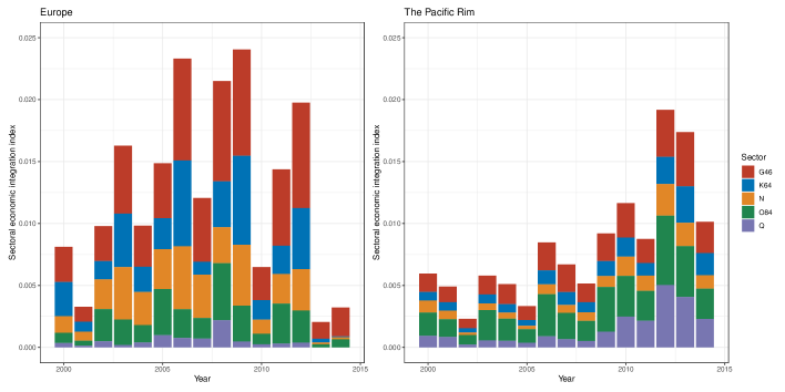
Fig 11: Sectoral economic integration index of other important sectors. G46: wholesale trade except that of motor vehicles and motorcycles; K64: financial service activities except insurance and pension funding; N: administrative and support service activities; O84: public administration and defense, and compulsory social security; Q: human health and social work activities.

Discussion

In the international trade networks used by Ikeda et al.[24], the communities are divided into industries; in original IVANs, the entire world is connected. Two buried communities—Europe and the Pacific Rim—were identified in the current paper by eliminating low flows with a threshold. However, since the IVAN included only 43 countries (excludes RoW), a more extensive international economic network, that is, one that includes other countries, may reveal more than two regional communities can.

The variability between the threshold and the community detection results is also important. In this study, we did not set the threshold as a specific weight in order to see the change over the 15 studied years. This is because the weights of IVAN links increase or decrease depending on economic growth or crisis; thus, it was inappropriate to use the same value as the threshold throughout the 15 years. In addition, as seen in Fig 1, the results of the detected communities are unstable, even for close threshold values. The threshold value did not separate the state of whether a single large community or two communities appeared; rather, the trend of the distribution changed. In this study, we used a resolution of every 500 links, but more detailed research is needed on the relationship between the number of remaining links and the number of detected communities. Thus, the threshold with the most remaining links was used for this analysis. The impact of this approach on the results is limited because the threshold was only applied for detecting concealed communities; it was not adopted for calculating the economic integration. With the threshold value we adopted, two communities with more than 240 nodes appeared, which is around 10% of the 2408 nodes included by the IVAN, and those communities were analyzed as regional communities. Therefore, the sector-specific European communities shown as gray nodes in Figs 2 and green small communities in 3 were not treated as the regional community of Europe. In other words, the European community does not include sector-specific European communities because Europe has substantial value flows that have mainly the same type of sector, not different types of sectors.

Originally, the smile curve [41] was viewed in terms of the production stage of a particular product or its relative position from a specific sector. In a broad sense, the smile curve in this study appears as a V-shaped curve when its relative position to the final goods of various sectors is considered as a whole. Not surprisingly, Helmholtz–Hodge decomposition shows a cross-country potential flow with high (low) potential in B: mining and quarrying (f: construction), which is in the upstream (downstream) stage of production. As seen from the circular relationship, the contributions of B: mining and quarrying and F: construction to international economic integration also indicate that the manufacture of each country depends on the resources and development demands (such as construction) of other countries.

To examine the implications of the economic integration index, we focused on the period of 2008–2011, which has exhibited substantial changes in economic integration (Fig 8); we also analyzed 2000 and 2014, which are the first and last years of the analyzed WIOD. Fig 12 shows the changes in the international and intersectoral relationships of circular flow in Europe. The circulation in 2008, the year of the highest integration index in Europe for the 15 years, is higher between Germany, France, Italy, and Russia compared with that in 2000. However, in 2011 and 2014, which has the lowest economic integration, Russia is absent in Europe, as shown in Tables 3 and 7. From a sectoral point of view, Fig 13 shows sector B: mining and quarrying as a hub of sectors F: construction; C19: manufacture of coke and refined petroleum products; and D35: electricity, gas, steam, and air conditioning supply. Therefore, the role of Russia and sector B: mining and quarrying is important for the high economic integration index in Europe.

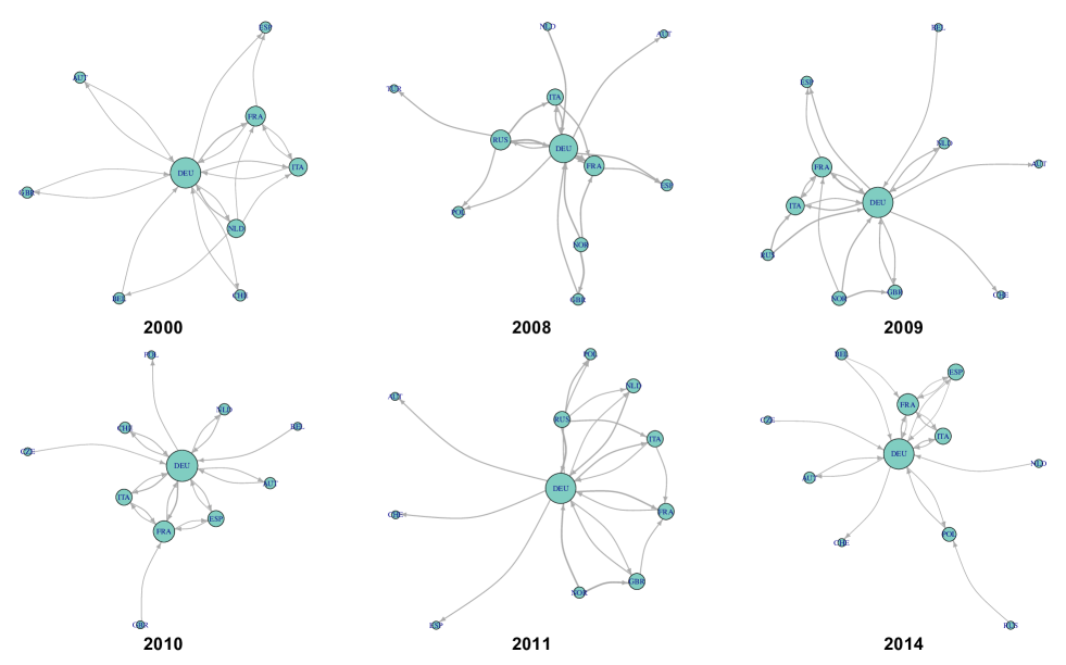
Fig 12: International value-added circulation of Europe in 2000, 2008–2011, and 2014. These graphs illustrate the top 20 links. Their node sizes and link widths are in proportion to the square root of the degree and the amount of circular flow, respectively. S1 Table. shows a detailed list of the sectors.

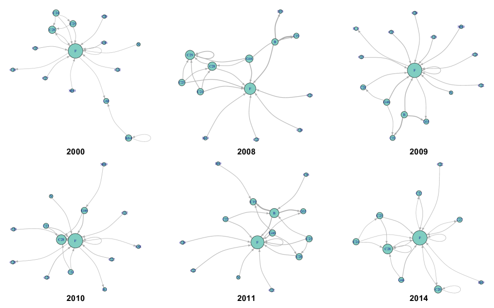
Fig 13: Intersectoral value-added circulation of Europe in 2000, 2008–2011, and 2014. These graphs illustrate the top 20 links. Their node sizes and link widths are in proportion to the square root of the degree and the amount of circular flow, respectively. S2 Table: List of sectors. shows a detailed list of the sectors.

Figs 14 and 15 show the changes in international and intersectoral relationships in the Pacific Rim. According to Fig 14, the center of the value-added circulation in the Pacific Rim changed from the United States and Japan to the United States and China. This also means that the Pacific Rim, as a regional community of IVANs, was detected stably because of the strong value-added circulation around the United States and China despite the economic crisis around 2009. From the sectoral perspective, Fig 15 shows that there are three crucial points in the circular structure of the Pacific Rim; these are the strongest stable circulations from B: mining and quarrying to F: construction, those within C26: manufacture of computer, electronic, and optical products, and those within C29: manufacture of motor vehicles, and trailers and semi-trailers for the years 2000–2014.

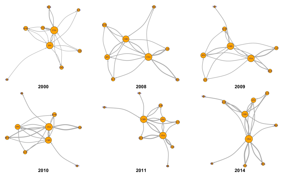
Fig 14: International value-added circulation of the Pacific Rim in 2000, 2008–2011, and 2014. These graphs illustrate the top 20 links. Their node sizes and link widths are in proportion to the square root of the degree and the amount of circular flow, respectively. S1 Table. shows a detailed list of the sectors.

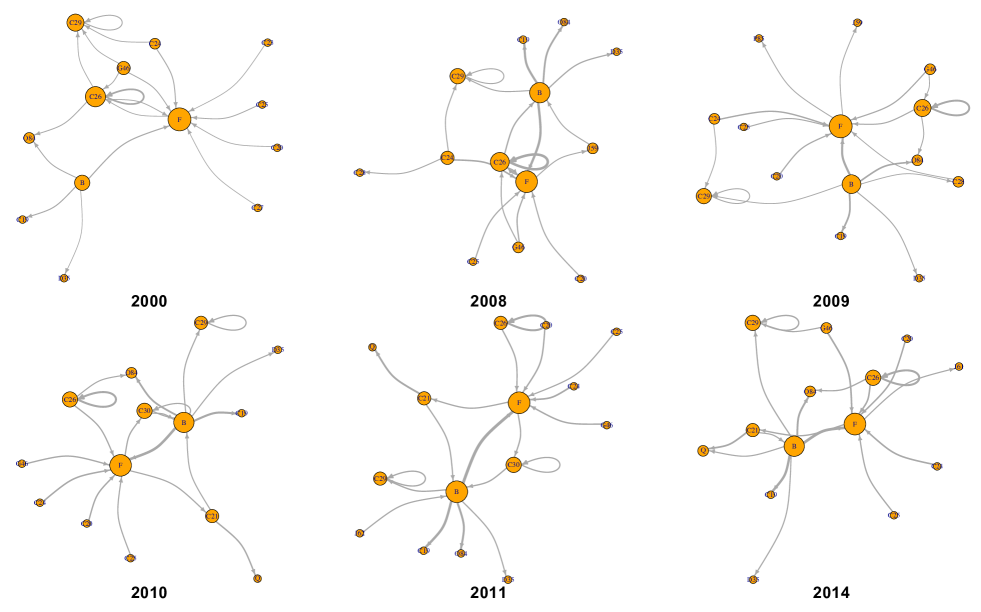
Fig 15: Intersectoral value-added circulation of the Pacific Rim in 2000, 2008–2011, and 2014. These graphs illustrate the top 20 links. Their node sizes and link widths are in proportion to the square root of the degree and the amount of circular flow, respectively. S2 Table: List of sectors. shows a detailed list of the sectors.

In Europe, the circulation between sectors B: mining and quarrying and F: construction is unstable because sector B mainly occurs in Russia, which is not an EU member country. Therefore, the extent of economic integration tends to be unstable. By contrast, the Pacific Rim has mineral resources. It also has neutral- and low-potential sectors with high circulation, namely, manufacture of high-tech and motor vehicles, respectively, which produces the high-value-added products as parts of GVCs.

These results suggest that the stable growth of economic integration in the Pacific Rim has been driven by the relationship of the value-added circulation of these resources and international division in the manufacture of high value-added products. Furthermore, in the Pacific Rim, the international division of labor is advancing, and value-added circulation is occurring across countries. This can be explained by the fact that, the free movement of labor in the EU has led to the specialization of sectors; in the Pacific Rim, the movement of labor is limited, and the international division of labor has led to the free movement of goods.

Conclusion

The purpose of this study is to clarify how international economic integration is occurring from the perspective of trade in value-added. For this purpose, we used the WIOD from 2016 to construct and analyze IVANs, which show the international relationship of sector-wise trade in value-added. First, the scope of economic integration was identified by Infomap, a community detection method that uses network flows. With threshold setting in the IVANs, regional communities in Europe and the Pacific Rim were detected throughout the 15 studied years. These two communities have not been found in studies that analyzed international trade networks constructed from the WIOD. To analyze how value flows within these two regions, we used Helmholtz–Hodge decomposition to extract the potential and circular relationships and clarified the annual changes in the roles played by the countries and sectors within these regions. In addition, we defined an economic integration index using the circular flow and applied it to both regions. We found that the level of economic integration in Europe, which had been increasing until 2008, dropped sharply after the economic crisis in 2009 to a level lower than that of the Pacific Rim in 2010, recovered in 2011, and dropped again after 2012 to a level below that of the Pacific Rim in 2013 and 2014. While the level of economic integration in Europe has been unstable, that in the Pacific Rim has been on a stable upward trend.

Moreover, the sectoral economic integration index provides a background to the changes in the extent of economic integration of these two regions. In Europe, the extent of economic integration declined in 2009, 2010, and 2013 due to the decrease of intra-European value-added circulation through the industries of mining, construction, petroleum, metal, machinery manufacture, wholesale, financial services, and management services, which showed a large amount of the circular flow of IVAN. This unstable extent of economic integration in Europe can be attributed to the fact that the free movement of labor within the EU has resulted in the connection of value-added circulation in specific sectors rather than the region as a whole. Meanwhile, in the Pacific Rim, economic integration is progressing slowly but steadily against the international vertical division of labor in sectors C26: manufacture of computer, electronic, and optical products, and C29: manufacture of motor vehicles. In the Pacific Rim, the international division of labor is believed to be developing stably because of the limited movement of labor.

Supporting information

S1 Table.

List of countries and regional classification. The table is in Appendix as Table 15.

S2 Table.

List of Sectors. The table is in Appendix as Table LABEL:S2_Tab.

Appendix

Table 15: Country list and regional classification.

ISO code	Short name	Region	ISO code	Short name	Region
AUS	Australia	Pacific Rim	IRL	Ireland	Europe
AUT	Austria	Europe	ITA	Italy	Europe
BEL	Belgium	Europe	JPN	Japan	Pacific Rim
BGR	Bulgaria	Europe	KOR	Korea	Pacific Rim
BRA	Brazil	Pacific Rim	LTU	Lithuania	Europe
CAN	Canada	Pacific Rims	LUX	Luxembourg	Europe
CHE	Switzerland	Europe	LVA	Latvia	Europe
CHN	China	Pacific Rim	MEX	Mexico	Pacific Rim
CYP	Cyprus	Europe	MLT	Malta	Europe
CZE	Czechia	Europe	NLD	Netherlands	Europe
DEU	Germany	Europe	NOR	Norway	Europe
DNK	Denmark	Europe	POL	Poland	Europe
ESP	Spain	Europe	PRT	Portugal	Europe
EST	Estonia	Europe	ROU	Romania	Europe
FIN	Finland	Europe	RUS	Russia	Pacific Rim
FRA	France	Europe	SVK	Slovakia	Europe
GBR	United Kingdom	Europe	SVN	Slovenia	Europe
GRC	Greece	Europe	SWE	Sweden	Europe
HRV	Croatia	Europe	TUR	Turkey	Europe
HUN	Hungary	Europe	TWN	Taiwan	Pacific Rim
IDN	Indonesia	Pacific Rim	USA	America	Pacific Rim
IND	India	Pacific Rim

Table 16: S2 Table: List of sectors.

Code	Description
A01	Crop and animal production, hunting and related service activities
A02	Forestry and logging
A03	Fishing and aquaculture
B	Mining and quarrying
C10	Manufacture of food products, beverages and tobacco products
C13	Manufacture of textiles, wearing apparel and leather products
C16	Manufacture of wood and of products of wood and cork except furniture,
	and manufacture of articles of straw and plaiting materials
C17	Manufacture of paper and paper products
C18	Printing and reproduction of recorded media
C19	Manufacture of coke and refined petroleum products
C20	Manufacture of chemicals and chemical products
C21	Manufacture of basic pharmaceutical products and pharmaceutical preparations
C22	Manufacture of rubber and plastic products
C23	Manufacture of other non-metallic mineral products
C24	Manufacture of basic metals
C25	Manufacture of fabricated metal products except machinery and equipment
C26	Manufacture of computer, electronic, and optical products
C27	Manufacture of electrical equipment
C28	Manufacture of machinery and equipment n.e.c.
C29	Manufacture of motor vehicles, trailers and semi-trailers
C30	Manufacture of other transport equipment
C31	Manufacture of furniture, and other manufacturing
C33	Repair and installation of machinery and equipment
D35	Electricity, gas, steam and air conditioning supply
E36	Water collection, treatment and supply
E37	Sewerage, waste collection, treatment and disposal activities, and materials recovery,
	and remediation activities and other waste management services
F	Construction
G45	Wholesale and retail trade and repair of motor vehicles and motorcycles
G46	Wholesale trade except that of motor vehicles and motorcycles
G47	Retail trade except that of motor vehicles and motorcycles
H49	Land transport and transport via pipelines
H50	Water transport
H51	Air transport
H52	Warehousing and support activities for transportation
H53	Postal and courier activities
I	Accommodation and food service activities
J58	Publishing activities
J59	Motion picture, video and television programme production, sound recording and
	music publishing activities; programming and broadcasting activities
J61	Telecommunications
J62	Computer programming, consultancy and related activities; information service activities
K64	Financial service activities, except insurance and pension funding
K65	Insurance, reinsurance and pension funding except compulsory social security
K66	Activities auxiliary to financial services and insurance activities
L68	Real estate activities
M69	Legal and accounting activities, and activities of head offices, and management
	consultancy activities
M71	Architectural and engineering activities, and technical testing and analysis
M72	Scientific research and development
M73	Advertising and market research
M74	Other professional, scientific and technical activities, and veterinary activities
N	Administrative and support service activities
O84	Public administration and defense, and compulsory social security
P85	Education
Q	Human health and social work activities
R_S	Other service activities
T	Activities of households as employers, and undifferentiated goods and services
	producing activities of households for own use
U	Activities of extraterritorial organizations and bodies

References

- 1. Hummels D, Ishii J, Yi K-M. The nature and growth of vertical specialization in world trade. Journal of International Economics 2001; Vol. 54.
- 2. Johnson RC, Noguera G. Accounting for intermediates: Production sharing and trade in value added. Journal of International Economics. 2012 doi: 10.1016/j.jinteco.2011.10.003.
- 3. Amador J, Cappariello R. Global value chains : a view from the EURO Area Asian Economic Journal 2015; 29(2), 99–120.
- 4. Koopman R, Wang Z, Wei S-J. TRACING VALUE-ADDED AND DOUBLE COUNTING IN GROSS EXPORTS. NBER WORKING PAPER SERIES 2012.
- 5. Dietzenbacher E, Los B, Stehrer R, Timmer M, de Vries G. THE CONSTRUCTION OF WORLD INPUT-OUTPUT TABLES IN THE WIOD PROJECT. Economic Systems Research. 2013 doi: 10.1080/09535314.2012.761180.
- 6. Timmer MP, Dietzenbacher E, Los B, Stehrer R, de Vries GJ. An Illustrated User Guide to the World Input-Output Database: The Case of Global Automotive Production. Review of International Economics. 2015, doi:10.1111/roie.12178.
- 7. Timmer MP, Dietzenbacher E, Los B., Stehrer R, de Vries GJ. User Guide to World Input–Output Database. Review of International Economics. 2015; 23: 575–605.
- 8. Cerina F, Zhu Z, Chessa A, Riccaboni M. World input-output network. PLoS ONE. 2015 doi: 10.1371/journal.pone.0134025.
- 9. Zhu Z, Puliga M, Cerina F, Chessa A, Riccaboni M. Global value trees. PLoS ONE, 2015; 10(5), 10-12. doi: 10.1371/journal.pone.0126699.
- 10. Los B, Timmer MP, de Vries GJ. HOW GLOBAL ARE GLOBAL VALUE CHAINS? A NEW APPROACH TO MEASURE INTERNATIONAL FRAGMENTATION. J. Regin. Sci., 2015; Vol. 55, No. 1, pp. 66–92.
- 11. Johnson RC, Noguera G. A portrait of trade in value-added over four decades. Review of Economics and Statistics, 2017; 99(5), 896–911.
- 12. World Bank. GLOBAL VALUE CHAIN DEVELOPMENT REPORT 2017: MEASURING AND ANALYZING THE IMPACT OF GVCs ON ECONOMIC DEVELOPMENT
- 13. World Bank. GLOBAL VALUE CHAIN DEVELOPMENT REPORT 2019: TECHNOLOGICAL INNOVATION, SUPPLY CHAIN TRADE, AND WORKERS IN A GLOBALIZED WORLD
- 14. Dollar D. Executive summary. Global Value Chain Development Report 2017, pp.1-14, The World Bank Group, Washington D.C.
- 15. Amador J, Cabral S. GLOBAL VALUE CHAINS: A SURVEY OF DRIVERS AND MEASURES. J. Econ. Surv., 2016; Vol. 30, No. 2, pp. 278–301.
- 16. Inomata S. Analytical frameworks for global value chains: An overview. Global Value Chain Development Report 2017, Chapter 1, The World Bank Group, Washington D.C.
- 17. Li X, Jin YY, Chen G. Complexity and synchronization of the World trade Web. Phys. A 2003; 328, 287–296.
- 18. Serrano MA, Boguna M. Topology of the world trade web. Phys. Rev. E 2003; 68, 015101.
- 19. Fagiolo G, Reyes J, Schiavo S. On the topological properties of the world trade web: A weighted network analysis. Phys. A 2008; 387, 3868–3878.
- 20. Fagiolo G, Reyes J, Schiavo S. World-trade web: Topological properties, dynamics, and evolution. Phys. Rev. E 2009; 79, 036115.
- 21. Foti NJ, Pauls S, Rockmore DN. Stability of the World Trade Web over time - An extinction analysis. Journal of Economic Dynamics & Control 2011; 37, 1889–1910.
- 22. Xiang L, Dong X, Guan J. Global industrial impact coefficient based on random walk process and inter-country input-output table. Physica A: Statistical Mechanics and Its Applications, 2017; 471, 576–591. doi: 10.1016/j.physa.2016.12.070.
- 23. Ikeda Y, Iyetomi H, Mizuno T, Ohnishi T, Watanabe T. Community structure and dynamics of the industry sector-specific international-trade-network. Proceedings - 10th International Conference on Signal-Image Technology and Internet-Based Systems, SITIS 2014, (4), 456–461.
- 24. Ikeda Y, Aoyama H, Iyetomi H, Mizuno T, Ohnishi T, Sakamoto Y, Watanabe T. Econophysics Point of View of Trade Liberalization : Community dynamics, synchronization. RIETI Discussion Paper Series 2016; 16-E-026.
- 25. Ikeda Y, Aoyama H, Sakamoto Y. Community dynamics and controllability of G7 global production network. In 2015 11th International Conference on Signal-Image Technology & Internet-Based Systems (SITIS) pp. 391–397. IEEE.
- 26. Aoyama H, Fujiwara Y, Ikeda Y, Iyetomi H, Souma W. Macro-Econophysics: New Studies on Economic Networks and Synchronization. Cambridge University Press, 2017/7/4, ISBN-13: 978-1107198951, chapter 6 and chapter 8
- 27. Barigozzi M, Fagiolo G, Manigioni G. Identifying the community structure of the international-trade multi-network Phys. A 2011; 390, 2051–2066.
- 28. De Benedictis L, Tajoli L. The World Trade Network. World Economy. 2011 doi: 10.1111/j.1467-9701.2011.01360.x.
- 29. Borchert I, Yotov YV. Distance, globalization, and international trade. Economics Letters. 2017, doi: 10.1016/j.econlet.2017.01.023.
- 30. Leontief WW. Quantitative input and output relations in the economic systems of the United States. The Review of Economics and Statistics. 1936; Vol. 18, No. 3, pp. 105–125. doi: 10.2307/1927837.
- 31. Stehrer R. Trade in Value Added and the Value Added in Trade. WIOD Working Paper 2012; 8, 1–19.
- 32. Rosvall M, Axelsson D, Bergstrom CT. The map equation. European Physical Journal: Special Topics 2009; 178(1), 13–23.
- 33. Fortunato S, Hric D. Community detection in networks: A user guide. Physics Reports, 2016; 659, 1-44. doi: 10.1016/j.physrep.2016.09.002.
- 34. Barabási A-L. Network Science. Cambridge University Press; 2016.
- 35. Huffman DA. A Method for the Construction of Minimum-Redundancy Codes. Proceedings of the I.R.E. 1952.
- 36. Rosvall M, Bergstrom. Maps of random walks on complex networks reveal community structure. PNAS, 2008; Vol. 105, No. 4, 1118-1123.
- 37. Lambiotte R, Rosvall M. Ranking and clustering of nodes in networks with smart teleportation. Physical Review E - Statistical, Nonlinear, and Soft Matter Physics, 2012; 85(5), 1-9. doi: 10.1103/PhysRevE.85.056107.
- 38. Shannon CE. A mathematical theory of communication. The Bell system technical journal, 1948;27(3), 379–423.
- 39. Bhatia H, Norgard G, Pascucci V, Bremer P-T. The Helmholtz-Hodge Decomposition—A Survey. IEEE TRANSACTIONS ON VISUALIZATION AND COMPUTER GRAPHICS, 2013 Aug. VOL. 19, NO. 8.
- 40. Kichikawa Y, Iyetomi H, Iino T, Inoue H. Community structure based on circular flow in a large-scale transaction network. Applied Network Science 2019; 4(1), 92.
- 41. Mudambi R. Location, control and innovation in knowledge-intensive industries. Journal of economic Geography, Volume 8, Issue 5, September 2008, Pages 699–725. doi: 10.1093/jeg/lbn024.