The emergence of Strange metal and Topological Liquid
near Quantum Critical Point in a solvable model

Abstract

We discuss quantum phase transition by an exactly solvable model in the dual gravity setup. By considering the effect of the scalar condensation on the fermion spectrum near the quantum critical point(QCP), we find that there is a topologically protected fermion zero mode associated with the metal to insulator transition. We also show that the strange metal phase with T-linear resistivity emerges at high enough temperature as far as the gravity has a horizon. The phase boundaries are calculated according to the density of states, giving insights on structures of the phase diagram near the QCP.

Introduction:

The quantum critical point (QCP) is believed to be a door to understanding strongly correlated systemsSachdev (2011). There, the particle characters are lost due to the interaction but the gravity dual description Maldacena (1999); Witten (1998); Gubser et al. (1998) may work due to the striking similarities between the QCP and the black hole: both get the universality by the apparent information loss, so that many different systems look the same. Both can be assigned with the spectral functions and transport coefficients so that it is likely that the we can identify the two if they are the sameLiu et al. (2013); Hartnoll et al. (2016). However, too many informations are lost at the QCP so that information about the QCP itself is not enough to identify a physical system and the properties off the QCP is essential.

Since the deriving force in the phase transition near the QCP typically is a symmetry breaking, we recently studied its effect on the fermion spectral function Oh et al. (2020) numerically. As a result, we found key features of quantum matters including the Fermi arc, flat band and nodal lines as well as the gap and pseudo gap. This is rather surprising since the topology is associated with clear band structure which usually become fuzzy in the strongly interacting system. So it raises unavoidable question: why this is related to the phenomena of appearance of the Fermi liquid in some of most strongly correlated system like heavy fermions. Answering theses question would provide a new angle to the study of the quantum matters with strong correlation.

In this paper we will show that there can be a gap or a zero mode with topological stability depending on the sign of the scalar field. See Figure 1(a) and (c).

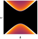
(a) $g\Phi>0,$ Gap

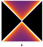
(b) $g\Phi=0,$ QCP

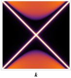
(c) $g\Phi<0,$ Gapless

Figure 1: Spectral Functions (a) for gapped phase, (b) for the QCP, (c) for the topological phase.

In fact, the appearance of the gapless mode in spite of the chiral symmetry breaking order is a surprise because it can never happen in the flat space field theory. It is also curious question to ask if an ordered state is gapless, how the order can be protected? We will see that it is the topological property and its presence is related to the parity invariance defined in Oh et al. (2020).

We will first demonstrate the presence of the zero mode by solving the Dirac equation analytically. We will then show that the fermion zero mode has the same mathematical structure with that of the topological insulator (TI). It is the anti-de Sitter space (AdS) version of the Jackiw-Rebbi solutionJackiw and Rebbi (1976). This also implies that the gapless phase is a dissipation free, hence we call it as the topological liquid (TL). Such topological character of the zero mode makes the TL different from the critical point in the spectrum: in Figure 1(c) there is clear separation between the gapped and the zero mode, which is characteristically different from the critical point of Figure 1(b) which shows a gapless fuzzy distribution of density of states.

The difference between the usual TI and and our system is that the zero mode in a usual TI describes a surface phenomena of the matter while it describes the bulk phenomena of the the physical matter here.

Because both gap and gapless phases are created out of a quantum critical point by a single order parameter with different sign, we interpret that it describes a phase transition at QCP from a (semi-) metal to insulator or its magnetic analogue. Indeed, when we turn on the temperature $T$ and calculate the spectral function as a function of the $T$, we found that the gapless phase has half width $\Gamma\sim T\sim 1/\tau$ which can be translated as the linear resistivity in $T$, signaling the presence of the strange metal. We will see that the so called Fermi liquid must exist in our theory as intermediate zone of the topological phase and the strange matter phase. We also find that the gapped phase also evolves to the strange metal as temperature goes high. It turns out that the presence of the zero modes is related to the fact that the gravity dual use the asymptotically anti de Sitter space which must have a boundary, and the appearance of the strange metal is associated with the presence of the black hole horizon.

An interesting aspect of our model is that the scalar is associated with the chiral symmetry breaking in the holographic space which does not break any obvious symmetry in the original space, which is a reminiscent of the situation in the spin liquid. It can provide a possibility that some of the orders which traditionally has not been associated with symmetry-breaking order may be associated with such order in higher dimensional holographic space. Our theory is applicable to the class of materials with transitions from insulator to topological (semi-)metal Brahlek et al. (2012); Salehi et al. (2016); Yang et al. (2014); Song et al. (2019). Finally, we suggest that the stable particle provided by the zero mode can make the Fermi liquid appear even in very strongly correlated system.

The fermion zero mode with scalar in AdS:

Let the bulk fermion $\psi$ be the dual field to the boundary fermion $\chi$ and $\Phi^{I}$ be the dual bulk field of the operator ${\bar{\chi}}\Gamma^{I}\chi$. We can encode the effect of the symmetry breaking on the spectrum of the fermions by consider the coupling $\bar{\psi}\,\Phi\cdot\Gamma\,\psi$ where $\Phi$ becomes a classical field under the symmetry breaking. The fermion equation of motion is given by $\left(\Gamma^{\mu}{\mathcal{D}}_{\mu}-m-g\Phi\right)\psi=0$ with $g=\pm 1$. The covariant derivative ${\cal D}_{\mu}$ is given by ${\cal D}_{\mu}=\partial_{\mu}+\frac{1}{4}\omega_{\mu ab}\Gamma^{ab}$. In this paper we use the simplest AdS black hole metric whose explicit form is given in the supplementary material A. In the zero temperature, $f=1$. For $m_{\Phi}^{2}=-2$ the solution for the scalar is given by $\Phi=M_{0}z+Mz^{2}$. In Poincare coordinate at zero temperature, both $M_{0}$ and $M$ can be independent boundary conditions, while for finite temperature with blackhole background, one of them is a boundary condition and the other is function of the other. Only when $M_{0}=0$, the value of $M$ is identified as the traditional condensation. The fact that $\Phi$ can include the non-zero source term $M_{0}$ which correspond to the external driving force is the important difference of the ’order parameter field’ in the holographic treatment. Physically $M_{0}$ can be related to the mass or doping parameter. One can check that the zero temperature solution remains good approximation even for finite temperature. This is because the large $z$ region where true solution deviates much from the probe solution is cut off by the presence of the horizon.

We can prove the existence of the zero modes by solving above Dirac equation explicitly. In the supplementary material A, the readers can find the analytic form of the Green functions at zero temperature whose pole give spectrum. For $\Phi=M_{0}z$, by analyzing the Green functions carefully we can see that the zero mode pole of $G^{g=1}_{R}$ is cancelled, while that of $G^{g=-1}_{R}$ survives. The massive particle spectra is given by $\omega^{2}-k^{2}=M_{0}^{2}\left(1-\frac{m^{2}}{(n+m+1)^{2}}\right)$ for both $g=\pm 1$ with $n=0,1,2\cdots$.

Similarly, for $\Phi=Mz^{2}$, the spectrum is given by $\omega^{2}-k^{2}=4M(n+m+1/2)$ for $g=1$ and $\omega^{2}-k^{2}=4Mn$ for $g=-1$. Notice that the first spectrum is gapful for any $n$, but the second one has a zero mode at $n=0$.

From these results, we see that for both $\Phi=M_{0}z$ and $\Phi=Mz^{2}$ cases, two completely different phases, one gaped and the other gapless, can emerge from the same quantum critical point at $g=0$ by invoking the scalar order depending the sign of the order parameter. This is a surprising aspect of AdS space because such phenomena never happen in flat space or in weakly interacting system where the scalar order introduces a gap, but not a zero mode. We want to understand its origin and implications.

The topological insulator in AdS:

The closest phenomena is the Jackiw-Rebbi (JR) fermion zero mode in the soliton background Jackiw and Rebbi (1976). It is a solution of the Dirac equation $(\gamma^{\mu}D_{\mu}-\varphi)\psi=0,$ where $\varphi$ changes sign across the domain wall. In such case the fermion has a normalizable zero mode, $\psi_{0}(x)=\exp{(-\int dx\varphi)}$ localized at the domain wall. Its stability is guaranteed by the boundary condition of $\varphi$ which makes $\varphi$ a topological soliton. See Figure 2(a)top. Much activities were performed under the name of the topological insulator after this solution is realized as the surface mode of condensed matter systems Hasan and Kane (2010); Qi and Zhang (2011). The configuration of $\varphi$ can be realized by the sign changing fermion mass across the boundary of the material, $\varphi=m\cdot{\rm sign}(x)$. See Figure 2(a)bottom.

Although we did not introduce any boundary of the physical system here, the gravity dual description use asymptotically Anti-de Sitter (AdS) space which has a boundary, that is identified with the physical space where the material is sitting.

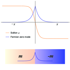
(a) Jackiw-Rebbi mode

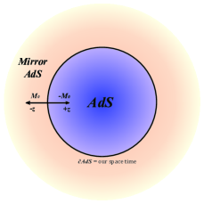
(b) JR mode in AdS

Figure 2: (a:top): Jackiw-Rebbi fermion zero mode in the soliton background. (a:bottom) Realization of the soliton $\varphi$ by sign changing mass. (b) $M_{0}$ corresponds to the $m$. The boundary of AdS is the bulk of the physical space.

Below, we will show that our zero mode solution can be considered as the JR mode in the AdS, which has a boundary at $z=0$ and its bulk is the region of $z>0$. The argument can be greatly simplified for the pure AdS limit where the Dirac equation becomes

$$\left[\Gamma^{z}\partial_{z}-iK_{\mu}\Gamma^{\mu}+\frac{m+g\Phi}{z}\right]\phi=0,$$ (1)

$\hbox{ with }K_{\mu}=(-\omega,k_{x},k_{y}).$ Now we consider $\chi_{0}(k)$ with $k=(\omega,{\bf k})$ satisfying $K_{\mu}\Gamma^{\mu}\chi_{0}(k)=0$, which is nothing but the Dirac equation with zero mass at the boundary of the AdS. Then $\chi_{0\pm}(k)$ defined by $\Gamma^{z}\chi_{0\pm}(k)=\pm\chi_{0\pm}(k)$ are also solutions. The zero mode in AdS can be constructed from this by $\phi_{0}(z,k)={\tilde{\phi}}(z)\chi_{0}(k)$, where $\tilde{\phi}$ is a scalar satisfying the eq.(1) for $K_{\mu}=0$. The solution is given by $\phi_{0}(z,x)=z^{-m}\exp(-g\int_{0}^{z}dz^{\prime}\varphi(z^{\prime}))\chi_{0+}+z^{m}\exp(g\int_{0}^{z}dz^{\prime}\varphi(z^{\prime}))\chi_{0-},$ where $\varphi=\Phi/z$ for $z>0$. The standard (alternative) quantization choose $\chi_{0+}$ ($\chi_{0-}$) Iqbal and Liu (2009); Laia and Tong (2011). By choosing $m<0$ and $g=-1$, the wave function in the bulk are normalizable and localized at $z=0$. One should also notice that $z^{\pm m}$ factor does not make an issue for the normalizability because $|m|<1/2$ by the unitarity boundIqbal and Liu (2009).

To make the parallelism with Jackiw-Rebbi solution describe above, we introduce the mirror AdS in the regime $z<0$. See Figure 2(b). The sufficient condition for the normalizability of the zero mode in $-\infty<z<\infty$, is $\varphi(-z)=-\varphi(z)$ which is clearly satisfied by

$$\varphi=M_{0}~{}{\rm sign}(z)+Mz.$$ (2)

It is instructive to consider the effect of each term in $\varphi$. Corresponding fermion zero modes are $\psi_{-0}^{(M_{0})}=|z|^{m}\exp(-M_{0}|z|)\chi_{0-}$ and $\psi_{-0}^{(M)}=|z|^{m}\exp(-\frac{1}{2}Mz^{2})\chi_{0-}$ respectively. They are zero modes localized at the boundary for $m<0$. The reader can read more explicit proof in the supplementary material E. Since the boundary of the AdS is the physical space bulk, our zero mode is the bulk mode of the real material unlike the TI in the weakly interacting system.

Summarizing, when there is a scalar condensation in the strongly interacting system, our theory predicts that there should be a topological liquid with non-dissipative zero mode, giving the metal or semi-metal depending on the size of the Fermi surface, which in turn can be tuned by the chemical potential.

Phase diagrams near the QCP:

Since both the gap and the gapless features are created out of a QCP by a single order parameter, there is a metal insulator transition at the QCP. Then, by adding the temperature, we can discuss the phase diagram near the quantum critical point. The dual of finite temperature is described by the black hole geometry. But we can use order parameter field which is the solution for for pure AdS as a leading approximation. To see the typical density of states(DOS) of each phases, we calculated the DOS numerically. Interested readers can see the Figure S1 of the supplementary material.

The density of state depends on the order parameter and temperature, and the shapes are quantitatively parametrized by the half width’s dependence on the two parameters. Therefore we can classify the phases according to $\Gamma$ as function of $T/M_{0}$. We can get the analytic result for it so that the entire phase diagram can be understood analytically.

The half width $\Gamma(T)$ of fermion density of state for AdS₄ with $\Phi=M_{0}z+Mz^{2}$ is given by,

$$\Gamma(T)={2\pi T}/{\int_{0}^{1}\frac{dtF(t)}{t(1-t)^{2/3}}},$$ (3)

with $F(t)=-\sinh[\frac{4m}{3}\tan^{-1}\!\!\sqrt{t}+{gM_{0}\beta_{0}(t)}/{T}+{gM\beta_{1}(t)}/{T^{2}}]$ where $\beta_{0}(t)=\frac{1}{2\pi}B(t;\frac{1}{2},\frac{1}{3})$ and $\beta_{1}(t)=\frac{3}{8\pi^{2}}B(t;\frac{1}{2},\frac{2}{3})$. Here $m$ is the bulk mass of the Dirac fermion in AdS₄, and in this paper we take $-1/2<m<0$. The derivation and more general result can be found in the supplementary materials C. Notice that when the temperature is much larger than the order parameter, $\Gamma\simeq\pi T/\gamma_{m},$ with $\gamma_{m}^{-1}=\frac{2m}{3}B(\frac{1}{2},\frac{1-2m}{3}){}_{3}F_{2}(\frac{1}{2},\frac{1}{2}-\frac{2m}{3},1-\frac{2m}{3};\frac{3}{2},\frac{1}{2}+\frac{1-2m}{3};1)$. We will give general argument later that this implies the appearance of the strange metal phase later. In the Figure 3, we plotted the half width in eq.(3) as function of $T$ for $gM_{0}=-2$.

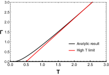
(a) $\Gamma(T)$ at $gM_{0}=-2$

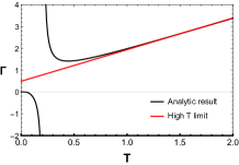
(b) $\Gamma(T)$ at $gM_{0}=+1$

Figure 3: (a,b) $\Gamma$ as a function of $T$. For high temperature, $\Gamma(T)\sim T$ universally. In (b) negative $\Gamma$ at low $T$ means the appearance of the gap there.

Phase boundaries can also be calculated by using eq. (3). The phase diagram in $(M_{0},T)$ plane is consequence of the competition of three regimes: i) Topological liquid whose core is the negative $M_{0}$ axis at $T=0$, ii)Gapped insulating phase whose core is at the positive $M_{0}$ axis. iii) the strange metallic phase whose center is defined by $a(T/M_{0}):=\frac{\partial\log\Gamma}{\partial\log T}=1$. It is along $T$ axis. We emphasize that these three lines are the center of the phases not phase boundaries. There is one true phase boundary in this phase diagram and it is $T^{*}$ line given by $T^{*}=M_{0}/m$ with $-1/2<m<0$, which is boundary between gapped and gapless regimes. The Figure 4(a) explains this idea. Notice that $M_{0}$ is not an order parameter but a source parameter so that it can be a parameter that can describe a phase diagram. See the Figure 4(b).

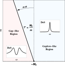
(a) structure of PD for $M_{0}$

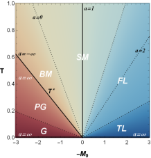
(b) phase diagram with $M_{0}$

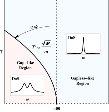
(c) structure of PD for $M$

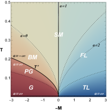
(d) phase diagram with $M$

Figure 4: True Phase transition exists only along $T_{*}$ lines. Others are crossover. In (b,d) ‘Fermi liquid(FL), strange metal(SM) and bad metal(BM)’ phases are around $a=2,1,0$ lines respectively.

Now the important point is that for $\Phi=M_{0}z$, $a(T,M_{0})=$constant lines where $\Gamma(T)\sim T^{a}$ are straight lines as it can be seen from eq.(3). As we rotate it starting from positive $-M_{0}$ axis counterclockwise, $a$ move from $\infty$ to $-\infty$ arriving at $T^{*}$ line. It should first pass the $a=2$ line where $\Gamma\sim T^{2}$, hence the core of the Fermi liquid phase. Then it pass the $a=1$ where $\Gamma\sim T$, the core of the strange metal phase. Upon the crossing the $T^{*}$ line, $a$ jumps from $-\infty$ to $\infty$. As we rotate further it decreases to arrive at the minimum and then increases to arrive at the negative $-M_{0}$ axis which is the core of insulating phase.

We define the phase boundary of the gapped and pseudo gap phases by the line at which $a$ is minimum. The resulting phase diagram is Figure 4(b). If we assume that the strength of the source $M_{0}$ is related with the doping rate $x$ by $M_{0}\propto(x_{0}-x)$, then our phase diagram mimic the that of the typical phase diagram near the QCP.

So far we confined ourselves to the order associated with explicitly broken symmetry with $\Phi=M_{0}z$ with $M=0$. We can repeat the analysis for the $\Phi=Mz^{2}$ with $M_{0}=0$. What is important is to notice that $\Gamma/T$ depends on the $M$ only through the combination $M/T^{2}$, and so is the exponent function $a(T)=\frac{d\log\Gamma}{d\log T}$. This means that all the phase boundary lines follow $T\propto\sqrt{M}$. We remark that we should consider $M$ as a boundary condition, not as a condensation. The latter is determined by setting $M_{0}=0$. The result is the Figure 4(c,d).

Emergence of the strange metal and the Fermi liquid with strong correlation

One can understand the emergence of the strange metallicity $\Gamma(T)\sim T$ directly from the equation of the motion (1). By rescaling $z=\zeta z_{H}$, the equation contains the temperature only in $\omega/T$ and inside $\Phi=(M_{0}z_{H})\zeta+(Mz_{H}^{2})\zeta^{2}$. For simplicity we consider the case $\Phi=M_{0}z_{H}\zeta$ only. When $M_{0}/T<<1$ the presence of the order can be neglected. Then the $T$ dependence comes only through $w:=\omega/T$. If the spectral width in $w$ in this case is $\Delta w=\Gamma_{0}$, then $\Gamma(T)$ defined as the spectral width in $\omega$ is given by $\Gamma(T)=\Delta\omega=T\Delta w=\Gamma_{0}T.$ Therefore $\Gamma(T)$ is linear in $T$ whatever is $\Gamma_{0}$. This explains the appearance of the strange metal for high temperature region in Figure 3(c): $\Gamma(T)\sim\hbar/\tau\sim T$ can be translated into the resistivity data $\rho\sim 1/\tau\sim T$.

Notice that the same argument can be applied to the equation describing the gauge field fluctuation in AdS space, and it gives the linear temperature dependence for the width of the Drude-like peak in the AC conductivity, which are also linear in $T$. It works as far as there is a horizon in the background gravity. This is the origin of the emergence of the strange metallicity.

When there is no order parameter, the strange metal appears even for $T\to 0$ limit, which explains why the strange metallic phase is of fan shape starting from the QCP in the phase diagram. The strange metal’s transport behavior has been discussed in the context of the holographic theory previously Faulkner et al. (2011, 2010); Blake and Tong (2013); Davison et al. (2014); Blake and Donos (2015); Ge et al. (2016). Our point is that apart from the existence of the black hole horizon and the temperature dominance over the order, we do not need anything else to prove it.

For low temperature regime, the kinetic term is very small compared with the interaction term: $|iK_{\mu}\Gamma^{\mu}|<<M_{0}\zeta$, therefore $M_{0}$ become the dominating scale and the system behavior follows the zero temperature physics. The zero mode that is responsible to our gapless mode is the Jackiw-Rebbi zero mode which has topological stability as we discussed before. This predicts the emergence of the topological liquid near zero temperature. The topological nature causes unusual stability of the Fermi-surface and it is expected that there is no dissipation in this phase. Such stability of the zero mode as a particle spectrum also predict that there should be a Fermi liquid phase in the system. One should also remember that the Fermi liquid phase in our theory appears as an intermediate region between the topological liquid and the strange metal. In heavy fermion system Fermi liquid is observed in spite of the strong correlation making the effective mass of the fermion 1000 times heavier. It would be interesting if we can connect our observation to such extraordinary stability of the Fermi liquid in terms of real data. We hope to come back to this issue soon.

Supplementary materials for

The emergence of Strange metal and Topological Liquid in a solvable model of Quantum Phase Transition:

Eunseok Oh, Taewon Yuk, Sang-Jin Sin^∗ Department of Physics, Hanyang University, Seoul 04763, Korea

Appendix A Spectrum and the zero modes with scalar order for $g=-1$

Here we show the presence of the zero mode by working out the full spectrum. Our fermion action is given by the sum $S=S_{g,A,\Phi}+S_{\psi}+S_{bdry}$, where

$$S_{g,A,\Phi} = \int d^{d+1}x\sqrt{-g}\left(R+\frac{6}{L^{2}}-\frac{1}{4}F^{2}_{\mu\nu}+D_{\mu}\Phi_{I}^{2}-m^{2}_{\Phi}\Phi^{2}\right),$$ (S1)

$$S_{\psi} = \int d^{d+1}\sqrt{-g}x\;i\bar{\psi}\left(\frac{1}{2}\Gamma^{\mu}(\overrightarrow{\mathcal{D}}_{\mu}-\overleftarrow{\mathcal{D}}_{\mu})-(m+g\Phi)\right)\psi,\,$$ (S2)

$$S_{bdy} = \pm\frac{i}{2}\int_{\partial M}d^{d}x\sqrt{-h}\bar{\psi}\psi.$$ (S3)

This action give the complete dynamics of all the fields including the Dirac field. According to the choice of sign of $S_{bdy}$, half of the bulk spinor degrees of freedom are projected out so that for $+(-)$ sign, only $\psi_{+}(\psi_{-})$ survive and this choice of the boundary action is called standard (alternative) quantizationFaulkner et al. (2013); Laia and Tong (2011). In this paper we use the simplest AdS black hole metric,

$$ds^{2}=-\frac{1}{L^{2}}\frac{f(z)}{z^{2}}dt^{2}+\frac{L^{2}}{z^{2}f(z)}dz^{2}+\frac{1}{L^{2}z^{2}}dx_{i}^{2},\quad f(r)=1-(\frac{{z}}{z_{H}})^{d-1},$$ (S4)

where the horizon radius is related to the temperature by $z_{H}=d/4\pi T$ and we set $L=1$. If we define $\phi_{\pm}(z)$ by $\psi_{\pm}=(-\det gg^{zz})^{-1/4}e^{-iwt+ik_{i}x^{i}}\phi_{\pm}(z)$, the $\phi$ satisfies

$$\left[\partial_{z}+\frac{1}{\sqrt{f}}\Big{(}iK_{\mu}\Gamma^{\mu}+\frac{m+g\Phi}{z}\Big{)}\Gamma^{z}\right]\phi=0,\hbox{ with }K_{\mu}=(-\omega/\sqrt{f},k_{x},k_{y}).$$ (S5)

Following the standard dictionary of AdS/CFT for the $p$-form bulk field $\Phi$ dual to the operator $O$ with dimension $\Delta$, its mass is related to the operator dimension by

$$m^{2}_{\Phi}=-(\Delta-p)(d-\Delta-p),$$ (S6)

and asymptotic form near the boundary is

$$\Phi=\Phi_{0}z^{d-\Delta-p}+\langle O_{\Delta}\rangle z^{\Delta-p}.$$ (S7)

We use following Gamma matrices representation Liu et al. (2011),

$$\Gamma^{r}=\sigma^{3}\otimes\mathbf{1}_{2},\quad\Gamma^{\mu}=\tau^{1}\otimes\gamma^{\mu},\hbox{ with }\gamma^{\mu}=\{i\sigma^{2},\sigma^{1},\sigma^{3}\},\hbox{ for }\mu=0,1,2.$$ (S8)

Case 1: $\Phi=Mz^{2}$

First we consider the case $\Phi=Mz^{2}$. Then the Dirac equation is equivalent to

$$-\phi_{\pm} {}^{\prime\prime}+\left(M^{2}z^{2}+\frac{m(m\pm 1)}{z^{2}}+2gM(m\mp\frac{1}{2})\right)\phi_{\pm}={\cal E}\phi_{\pm},$$ (S9)

where ${\cal E}={w^{2}-\vec{k}^{2}}$. The solution to the eq.(S9) is given by

$$\phi_{+} =2^{\frac{1}{2}(\frac{1}{2}-m)}z^{-m}e^{-M\frac{z^{2}}{2}}\left(\mathbf{C}_{1+}U^{\frac{1}{2}-m}_{u}(Mz^{2})+\mathbf{C}_{2+}L^{-\frac{1}{2}-m}_{-u}(Mz^{2})\right)$$ (S10)

$$\phi_{-} =2^{\frac{1}{2}(\frac{1}{2}+m)}z^{m}e^{-M\frac{z^{2}}{2}}\left(\mathbf{C}_{1-}U^{\frac{1}{2}+m}_{v}(Mz^{2})+\mathbf{C}_{2-}L^{-\frac{1}{2}+m}_{-v}(Mz^{2})\right)$$ (S11)

$$\hbox{with }\varepsilon =\frac{w^{2}-\vec{k}^{2}}{4M},u=\frac{1}{2}(g-1)(m-\frac{1}{2})-\varepsilon,\;v=\frac{1}{2}(g+1)(m+\frac{1}{2})-\varepsilon,$$ (S12)

$$U_{u}^{k}(z)= z^{-u}{}_{2}F_{0}(u,1+u-k;;-z^{-1}),\;L_{u}^{k}(z)=\frac{\Gamma(k+1+u)}{\Gamma(k+1)\Gamma(u+1)}{}_{1}F_{1}(-u,k+1;z)$$ (S13)

where $\mathbf{C}_{i\pm}$ are two component constant spinors and $U_{u}^{k}$ and $L_{u}^{k}$ are associated Laguerre, whose asymptotic behavior determines the normalizability of $\psi$. Since the Laguerre function $L_{u}^{k}$ in general contains $e^{Mz^{2}}$ we need to set $\mathbf{C}_{2\pm}=0$. The $z\rightarrow\infty$ behaviors are

$$\phi_{+} \sim{2^{\frac{1}{4}-\frac{m}{2}}e^{-\frac{Mz^{2}}{2}}z^{-2u-m}\mathbf{C}_{1+}M^{-u}},$$

$$\phi_{-} \sim{2^{\frac{1}{4}+\frac{m}{2}}e^{-\frac{Mz^{2}}{2}}z^{-2v+m}\mathbf{C}_{1-}M^{-v}}.$$ (S14)

Then, $z\rightarrow 0$ behaviors are given by

$$\phi_{+}\sim 2^{\frac{1}{4}-\frac{m}{2}}\left(z^{-m}B_{1+}+z^{m+1}B_{2+}\right),\quad\phi_{-}\sim 2^{\frac{1}{4}+\frac{m}{2}}\left(z^{1-m}B_{1-}+z^{m}B_{2-}\right)$$ (S15)

$$\hbox{ where }\quad B_{1+} =\mathbf{C}_{1+}\frac{\Gamma(m+{1}/{2})}{\Gamma(u+m+{1}/{2})},\quad\quad\quad\quad\;\,B_{2+}=\mathbf{C}_{1+}M^{{1}/{2}-m}\frac{\Gamma(-{1}/{2}-m)}{\Gamma(u)},$$ (S16)

$$B_{1-} =\mathbf{C}_{1-}M^{{1}/{2}-m}\frac{\Gamma(m-{1}/{2})}{\Gamma(u+m+{g}/{2})},\quad B_{2-}=\mathbf{C}_{1-}\frac{\Gamma\left({1}/{2}-m\right)}{\Gamma(u+{(g+1)}/{2})}.$$ (S17)

The relation

$$B_{2-}=i(2m+1)\frac{\gamma^{\mu}k_{\mu}}{w^{2}-{k}^{2}}B_{2+},\quad B_{1-}=i(2m-1)\frac{\gamma^{\mu}k_{\mu}}{w^{2}-{k}^{2}}B_{1+}$$ (S18)

which was established in Liu et al. (2011) still hold here in the presence of the interaction term. Then the Green Function $G_{R}$ is defined by

$$G_{R}=-iS\gamma^{0},\quad\hbox{ with S defined by }B_{2-}=SB_{1+}.$$ (S19)

Now we can write down Green functions for each sign of $g$.

$$G^{g=1}_{R} = M^{-1/2+m}\frac{\Gamma(\frac{1}{2}-m)\Gamma(\frac{1}{2}+m-\varepsilon)}{2\Gamma(\frac{1}{2}+m)\Gamma(1-\varepsilon)}\gamma^{\mu}k_{\mu}\gamma^{t},$$ (S20)

$$G^{g=-1}_{R} = M^{-1/2+m}\frac{\Gamma(\frac{1}{2}-m)\Gamma(-\varepsilon)}{2\Gamma(\frac{1}{2}+m)\Gamma(\frac{1}{2}-m-\varepsilon)}\gamma^{\mu}k_{\mu}\gamma^{t}.$$ (S21)

The poles of the Green function are given by those of gamma function at the non positive integers so that the spectra are given by

$$\omega^{2}-k^{2} = 4M(n+m+1/2),\hbox{ for }g=1,$$ (S22)

$$\omega^{2}-k^{2} = 4Mn,\hbox{ for }g=-1,$$ (S23)

with $n=0,1,2,\cdots$. The first spectrum is gapful for any $n$, but the second one has the zero mode at $n=0$.

Case 2: $\Phi=M_{0}z$

Now we turn to the case $\Phi=M_{0}z$. The equation of motion for $\phi$ with scalar source $M_{0}$ is equivalent to

$$-\phi_{\pm} {}^{\prime\prime}+\left(\frac{m(m\pm 1)}{z^{2}}+M_{0}^{2}+g\frac{2mM_{0}}{z})\right)\phi_{\pm}={\cal E}\phi_{\pm}.$$ (S24)

After fixing the coefficients to remove the divergent pieces in $z\rightarrow\infty$ limit, the solution is

$$\phi_{\pm} = e^{-\sqrt{\mu}z}(2\sqrt{\mu}z)^{\mp m}U_{\mp m+g\nu}^{\mp 2m}(2\sqrt{\mu}z)$$ (S25)

$$\mu = k^{2}-w^{2}+M_{0}^{2},\quad\nu=\frac{m}{\sqrt{1-\varepsilon^{\prime}}},\quad\varepsilon^{\prime}=\frac{\omega^{2}-k^{2}}{M_{0}^{2}}.$$ (S26)

The $z\rightarrow 0$ behavior of the solution is

$$\phi_{+} \sim z^{-m}\frac{(2\sqrt{\mu})^{-m}\Gamma(1+2m)}{\Gamma(1+m+g\nu)}+z^{1+m}\frac{(2\sqrt{\mu})^{1+m}\Gamma(-1-2m)}{\Gamma(-m+g\nu)}$$ (S27)

$$\phi_{-} \sim z^{1-m}\frac{(2\sqrt{\mu})^{1-m}\Gamma(2m-1)}{\Gamma(m+g\nu)}+z^{m}\frac{(2\sqrt{\mu})^{m}\Gamma(1-2m)}{\Gamma(1-m+g\nu)}.$$ (S28)

These data give the Green functions for $\Phi=M_{0}z$:

$$G^{g=1}_{R} = \frac{(4{\mu})^{\frac{1}{2}+m}\Gamma(-2m)\Gamma\left(1+m+\nu\right)}{\left(k^{2}-w^{2}\right)\Gamma(-m+\nu)\Gamma(1+2m)},$$ (S29)

$$G^{g=-1}_{R} = \frac{(4{\mu})^{\frac{1}{2}+m}\Gamma(-2m)\Gamma\left(1+m-\nu\right)}{\left(k^{2}-w^{2}\right)\Gamma\left(-m-\nu\right)\Gamma(1+2m)}.$$ (S30)

where parameters $\mu,\nu$ are given by $\mu=k^{2}-w^{2}+M_{0}^{2}$ and $\nu=\frac{m}{\sqrt{1-\varepsilon^{\prime}}}$ with $\varepsilon^{\prime}=\frac{\omega^{2}-k^{2}}{M_{0}^{2}}$. Although these two look similar, there is a striking difference: notice that $(k^{2}-w^{2})\Gamma(-m+\nu)\approx-2M_{0}^{2}/m$ near the lightcone $k^{2}=\omega^{2}$, therefore the apparent zero mode pole of $G^{g=1}_{R}$ is cancelled, while the zero mode of $G^{g=-1}_{R}$ survives. The massive particle spectra exist only for $m<0$ if $g=1$, while they exist only for $m>0$ if $g=-1$. In both cases, the massive tower is given by

$$\omega^{2}-k^{2}=M_{0}^{2}\left(1-\frac{m^{2}}{(n+m+1)^{2}}\right),\;\;n=0,1,2\cdots.$$ (S31)

The spectra given in eq. (S23) and (S31) are the Kaluza Klein tower associated with the box character of AdS space, which gives an effective compactification.

Appendix B Typical Density of States for various phases

To see the typical density of states(DOS) of each phases, we calculated the DOS numerically. The Figure S1 is result of this.

(a) Topological Liquid

(b) Strange Metal

(c) Gap

(d) Pseudo-gap

Figure S1: DOS for different phases $\Gamma(T)$ for $m=-0.3$: For (a,b) $T=0.1,0.8$ respectively along $gM_{0}=-2$. For (c,d) $T=0.01,0.15$ respectively along $gM_{0}=1$. In Figure (c) $\Gamma<0$ for the gap.

Appendix C Analytic expression for $\Gamma(T)$

To calculate the $\Gamma$ as a function of the temperature, we define the spectral function $\cal A$ by

$$\mathcal{A}=\textrm{Tr}(\textrm{Im}G_{R})$$ (S32)

and expand $\mathcal{A}$ for small $w$ by,

$$\mathcal{A} =\mathcal{A}^{(0)}(1-\tau w+\cdots)$$ (S33)

$$=\mathcal{A}^{(0)}+w\mathcal{A}^{(1)}+\cdots$$ (S34)

Then the relaxation time $\tau$ is defined by the small $w$ expansion

$$\tau=\frac{1}{\Gamma}=-\frac{\mathcal{A}^{(1)}}{\mathcal{A}^{(0)}}$$ (S35)

The Dirac equation S5 is equivalent to the flow equation for $\xi_{\pm}$ as follows

$$\left(\partial_{z}+2\frac{g\Phi+m/z}{\sqrt{f(z)}}\right)\xi_{\pm}(z)=\left(\frac{w}{f(z)}\pm\frac{k}{\sqrt{f(z)}}\right)\xi_{\pm}(z)^{2}+\left(\frac{w}{f(z)}\mp\frac{k}{\sqrt{f(z)}}\right)$$ (S36)

where $\xi_{+}=\frac{iy_{-}}{z_{+}},\xi_{-}=-\frac{iz_{-}}{y_{+}}$ and $\phi_{\pm}=(y_{\pm},z_{\pm})^{T}$. The retarded Green function $G_{R}=z^{2m}{\rm diag}(\xi_{+},\xi_{-})|_{z\to 0}$Liu et al. (2011). From now on we set $k=0$, so that the equations for $\xi_{+}$ and $\xi_{-}$ are the same for $k=0$ and we delete the lower index $\pm$ from $\xi_{\pm}$. Now, we expand the $\xi$ in $w$ up to first order,

$$\xi(z)=\xi^{(0)}(z)+w\xi^{(1)}(z)+\cdots.$$ (S37)

Substituting the eq. S37 into eq. S36, the equations for the zero-th and first order in w expansion becomes

$$(\partial_{z}+2\frac{g\Phi+m/z}{\sqrt{f(z)}})\xi^{(0)}(z)=0,$$ (S38)

$$(\partial_{z}+2\frac{g\Phi+m/z}{\sqrt{f(z)}})\xi^{(1)}(z)=\frac{1+\xi^{(0)}(z)^{2}}{f(z)}.$$ (S39)

The in-falling boundary conditions at the horizon implies $\xi^{(0)}(z_{H})=i,\,\xi^{(1)}(z_{H})=0$. We now can calculate the decay rate $\Gamma$ using

$$\Gamma=-\frac{\mathcal{A}^{(0)}}{\mathcal{A}^{(1)}}=-\frac{\textrm{Im}\xi^{(0)}(z)}{\textrm{Im}\xi^{(1)}(z)}\Big{|}_{z\to 0}.$$ (S40)

case $m\neq 0$

A decay rate $\Gamma$ for AdS_d+1 with $\Phi=M_{0}z+Mz^{2}$ is given by,

$$\Gamma(T)= \frac{2\pi T}{\int_{0}^{1}dt(1-t)^{(1/d-1)}{F(t)}/{t}},$$ (S41)

$$\textrm{ with }F(t)=-\sinh[\frac{4m}{d}\tan^{-1}\!\!\sqrt{t}+\frac{gM_{0}\beta_{0}(t)}{T}+\frac{gM\beta_{1}(t)}{T^{2}}],$$ (S42)

where $\beta_{0}(t)=\frac{1}{2\pi}B(t;\frac{1}{2},\frac{1}{d}),\quad\beta_{1}(t)=\frac{d}{8\pi^{2}}B(t;\frac{1}{2},\frac{2}{d})$. Notice that in this paper we take $-1/2<m<0$. This result explains the appearance of the strange metallicity at the critical point and near by region. At the criticality where the order parameters are zero, the appearance of the strange metalicity is equivalent to the presence of the black hole horizon, which in turn is equivalent to the presence of the scrambling power of the chaotic fluctuation of the quantum critical point. However, the appearance of other phases is consequence of the symmetry breaking. Such competition of the strange metallicity, or chaos, and the order determines the shape of the phase diagram near the QCP. Notice that

$$\Gamma\simeq\pi T/\gamma_{m,d},\quad\hbox{ at }T>>\sqrt{M},M_{0},$$ (S43)

with

$$\gamma_{m,d}^{-1}=\frac{2m}{d}B(\frac{1}{2},\frac{1-2m}{d}){}_{3}F_{2}(\frac{1}{2},\frac{1}{2}-\frac{2m}{d},1-\frac{2m}{d};\frac{3}{2},\frac{1}{2}+\frac{1-2m}{d};1).$$

For $d=1,2$, we have simple result $\gamma_{d}=\frac{\pi}{2}\tan(m\pi)$. We used eq. (S42) to calculate the phase boundaries.

One may want to compare above analytic result with numerical calculation to check its validity. The result is Figure S2, showing that our formula agrees with numerical calculation precisely.

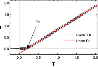
(a) $M=-2$

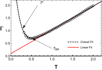
(b) $M=1$

Figure S2: $\Gamma(T)$ for $m=-0.4$: For (a) $M=-2$ (b)$M=1$ respectively. Numerical $\Gamma$ is defined by a half width of spectral function at $w=0$

case $m=0$

For $m=0$, the spectral function $\mathcal{A}$ has non zero asymptotic value, i.e. $\lim_{\omega\to\infty}{\rm Im}G(\omega)=1$. Therefore, the usual definition does not work. To overcome, we define the Drude function $\mathcal{A}_{D}$ by $\mathcal{A}_{D}=\mathcal{A}-1$. Then the relaxation time $\tau$ is defined by the small $\omega$ expansion $\mathcal{A}_{D}(w)\sim\mathcal{A}_{D}(0)(1-\tau w+\cdots),$ so that $\tau=\frac{1}{\mathcal{|A_{D}|}}\frac{\partial{\mathcal{A_{D}}}}{\partial{w}}|_{w=0}.$ Obviously negative-$\Gamma$ can be interpreted as a measure of the gap. With this preparation, we get the following formula for $m=0$ for $AdS_{d+1},d>1$:

$$\Gamma=2\pi T\frac{(e^{\frac{\alpha gM_{0}}{T}}-1)}{\int_{0}^{1}(1-t)^{(1/d-1)}\frac{\sinh\left(gM_{0}\beta_{0}(t)/T\right)}{t}dt},$$ (S44)

where $\alpha=\frac{1}{2\pi}B(\frac{1}{2},\frac{1}{d}),\quad\beta_{0}(t)=\frac{1}{2\pi}B(t;\frac{1}{2},\frac{1}{d})$. Notice that for the large T, the width is also reduced to linear in $T$ : $\Gamma\simeq\frac{\pi T}{\gamma_{d}}$, with $\gamma_{d}={}_{3}F_{2}(\frac{1}{2},\frac{1}{2},1-\frac{1}{d};\frac{3}{2},\frac{1}{2}+\frac{1}{d};1)$.

Similarly, for the condensation, the decay rate with the scalar condensation is

$$\Gamma =2\pi T\frac{(e^{\frac{\alpha^{\prime}gM}{T^{2}}}-1)}{\int_{0}^{1}(1-t)^{(1/d-1)}\frac{\sinh\left(gM\beta^{\prime}(t)/T^{2}\right)}{t}dt}$$ (S45)

where $\alpha^{\prime}=\frac{d}{8\pi^{2}}B(\frac{1}{2},\frac{2}{d}),\,\beta^{\prime}(t)=\frac{d}{8\pi^{2}}B(t;\frac{1}{2},\frac{2}{d}),$ $\Gamma\simeq\frac{\pi T}{\gamma^{\prime}_{d}}$ in the large T limit, with

$$\gamma^{\prime}_{d}=\sqrt{\pi}{2^{1-\frac{2}{d}}}\frac{\Gamma(\frac{1}{2}+\frac{2}{d})}{{\Gamma(\frac{1}{2}+\frac{1}{d})}^{2}}\cdot{}_{3}F_{2}(\frac{1}{2},\frac{1}{2},1-\frac{2}{d};\frac{3}{2},\frac{1}{2}+\frac{2}{d};1).$$

We tabulated $\gamma_{d}$ and $\gamma^{\prime}_{d}$ in Table 1 explicitly.

d	1	2	3	4
$\gamma_{d}$	1	1.1662	${\sqrt{3}\pi}/{4}$	${\pi}/{2}$
$\gamma^{\prime}_{d}$	$\frac{7}{5}$	${\pi}/{2}$	1.7538	1.9468

Table 1: $\gamma_{d}$ and $\gamma^{\prime}_{d}$ for AdS${}_{d+1},\quad d=1,2,3,4$.

Appendix D Comment on the conformal factor $z^{\pm m}$

The point we want to make below is that $z^{\pm m}$ is not the factor that counts probability of location but the conformal factor to embed the boundary theory into the AdS bulk, which we should delete in probability interpretation of locality. To see why this is so, we remind the basic dictionary of the AdS/CFT for scalar case: if a scalar operator of dimension $\Delta$ couple to the source $\phi_{0}(x)$, then the bulk field dual to the operator, $\Phi(z,x)$, is NOT given by the direct extension of the $\phi_{0}$. Due to the conformal structure of AdS spaceWitten (1998), we need to dress the source and response by the conformal factor $z^{\Delta_{\mp}}$ such that two independent solutions of the bulk field $\Phi$ are given by $\Phi(z,x)=\phi_{0}(x)z^{\Delta_{-}}(1+\cdots)$ and $\Phi(z,x)=\langle O\rangle z^{\Delta_{+}}(1+\cdots)$, where $\Delta_{\pm}$ are the solutions of $\Delta(\Delta-d)=m_{\Phi}^{2}$. The equation of motion for $\Phi$ is of second order so that the general solution is given by the linear combination of the two. Conversely, in other to read off the ‘extended configuration of $\phi_{0}$’ from the solution of the bulk equation of motion, we need to strip off the factor $z^{\Delta_{\pm}}$ from the first and second solutions. Therefore, we define the undressed physical source/response bulk field $\Phi_{u,s},\Phi_{u,r}$ by dividing out the conformal factor from the corresponding solutions of the bulk equation of motion.

Similarly for the spinor fields $\psi=(\psi_{+},\psi_{-})^{T}$, we can define the undressed source and response functions by $\psi_{\pm}=z^{\Delta_{\mp}}\psi_{u\pm}$ with $\Delta_{\pm}=3/2\pm m$. It is worthwhile to mention that the boundary Green functions are given by the ratio of these undressed wave functions for both bosons and fermions. Then we can show that the normalizable undressed wave function is localized at the boundary and only the zero mode has such property.

Appendix E Localization of zero modes at the AdS boundary

Coming back to the AdS plus mirror space, the undressed wave function for the zero mode is

$$\psi_{0u+}\simeq e^{-M_{0}|z|},\hbox{ for }-\infty<z<\infty.$$ (S46)

This is precisely the Jackiw-Rebbi’s normalizable soliton solution localized at the domain wall $z=0$ where the kink configuration is realized by term $M_{0}{\rm sign}(z)$. It also means that our zero mode can be considered as the edge state of a virtual topological insulator. However, we should not forget that our zero mode describe the bulk mode since it is free to move along the boundary of the AdS, which is the bulk of the physical world. In all these discussion, we introduced the mirror AdS to take direct similarity of JR solution. However one should notice that all that is used is to have the refection symmetry of the wave equation and a non-vanishing Dirichlet boundary condition of the undressed wave function $\psi_{u\pm}$ at $z=0$.

For $\Phi=Mz^{2}$ and the equation of motion (S9) is invariant under $z\to-z$ without sign change of $M$. The ground state given by

$$\psi_{+}\simeq e^{-{Mz^{2}}/{2}},$$ (S47)

which is the zero mode localized at the domain wall at $z=0$.

One might think that any state are localized the boundary of the AdS. Below, we will show only the ground state for $g=-1$ is localized while all other states are not. To see this, notice that

$$\psi^{g=1}_{u+}(z=0) \sim 2^{\frac{1}{4}-\frac{m}{2}}\frac{\Gamma(\frac{1}{2}+m)}{\Gamma(-n)}=0,\hbox{ for any integer }n\geq 0,$$ (S48)

$$\psi^{g=-1}_{u+}(z=0) \sim 2^{\frac{1}{4}-\frac{m}{2}}\frac{\Gamma(\frac{1}{2}+m)}{\Gamma(1-n)}>0,\hbox{ for }n=0,$$ (S49)

which shows clearly the uniqueness of the zero mode for $g=-1$. For a massive mode with $n\geq 1$, the wave functions are not localized for two reasons: first, the wave functions vanish at $z=0$ and secondly they oscillate and penetrates into larger $z$ region. The larger is $n$, the deeper it penetrates. See the Figure S3. As far as $M$ or $M_{0}$, which is the gap between the ground state and the others, is non-zero, there exists a fermion zero mode for $g=-1$ so we may say that the fermion zero mode is protected by the presence of the gap, therefore we call the symmetry broken phase with $g=-1$ as ‘topological liquid’. The point we want to make is that the zero mode has a topological character, and as such, it has to do with a phenomena which looks like Fermi liquid but with an unusual stability.

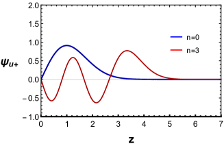
(a) $g=1$

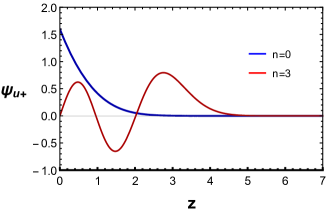
(b) $g=-1$

Figure S3: wave function for $M=1,m=0$ for various modes. Only the ground state for $g=-1$ state is localized at the boundary of the AdS.