Exergy-based modeling framework for hybrid and electric ground vehicles

Abstract

Exergy, or availability, is a thermodynamic concept representing the useful work that can be extracted from a system evolving from a given state to a reference state. It is also a system metric, formulated from the first and the second law of thermodynamics, encompassing the interactions between subsystems and the resulting entropy generation. In this paper, an exergy-based analysis for ground vehicles is proposed. The study, a first to the authors’ knowledge, defines a comprehensive vehicle and powertrain-level modeling framework to quantify exergy transfer and destruction phenomena for the vehicle’s longitudinal dynamics and its energy storage and conversion devices (namely, electrochemical energy storage, electric motor, and ICE). To show the capabilities of the proposed model in quantifying, locating, and ranking the sources of exergy losses, two case studies based on an electric vehicle and a parallel hybrid electric vehicle are analyzed considering a real-world driving cycle. This modeling framework can serve as a tool for the future development of ground vehicles management strategies aimed at minimizing exergy losses rather than fuel consumption.

1 Introduction

Greenhouse gas emissions reduction and efficiency improvement are fundamental challenges that must be solved to promote sustainability in the transportation sector. Vehicle electrification, in the form of Electric Vehicles (EVs) and Hybrid Electric Vehicles (HEVs), has shown to be the key towards the development of efficient technologies to minimize both powertrain losses and carbon footprint. The design of novel powertrain architectures that meet the above requirements has been traditionally carried out from energy-based analysis. This methodology, however, does not allow for the formal quantification of losses, limiting the further vehicle and powertrain-level optimization.

On the other hand, exergy, or availability, allows for the quantification of the useful work available to a system and of the associated irreversibilities. Exergy is an overall system metric that encompasses the interactions between subsystems, and it is formulated upon the first and the second laws of thermodynamics. Exergy is not simply a thermodynamic property of a system, it is also a metric defined with respect to a reference state: the ability to do work depends upon both the given state of the system and its surroundings. Therefore, the exergy content of a system can change even if the state of the system does not, for instance, if the external temperature varies with respect to the initial condition [1]. This fundamental characteristic enables the exergetic analysis of systems interacting with their surroundings.

Availability was first applied to analyze losses in chemical processes and power applications [2]. Soon after, exergy-based modeling became a powerful tool to assess the overall system performance and help the engineering and designing process in other fields. For instance, applications of availability analysis can be found for gas turbines [3], [4], solar technology [5], [6], nuclear and coal-fired plants [7], [8], and conversion and storage electrical energy systems [9].

In the aerospace field, a plethora of work on exergy-based analysis applied to aircrafts, rockets, and launch vehicles can be found. In particular, [1] and [10] apply exergy for the design, analysis, and optimization of hypersonic aircrafts. In [11] and [12], exergy modeling of rockets and launch vehicles is tackled, respectively. Recent works also show the application of availability to quantify the sources of loss within ships’ energy systems. According to [13], this information could be used to further reduce the environmental impact and greenhouse gas emissions in maritime transport.

Exergy analysis has been widely used also in Internal Combustion Engines (ICEs). The ICE is a complex device, composed of many interacting parts (up to 2000), subject to losses originated from frictions, heat exchange, and suboptimal combustion. In this framework, exergy can be used to optimize combustion and, consequently, braking work generation. Concerning the spark-ignition technology, [14] and [15] analyze the exergy transfer and destruction phenomena for synthetic and natural gas fueled engines, respectively. In [16], an overview on availability modeling of naturally aspirated and turbocharged diesel engines is provided. In [17], the authors prove that, for a homogeneous charge compression ignition engine, $6.7\%$ of fuel can be saved by implementing an exergy-based Model Predictive Control (MPC) strategy (with respect to a suboptimal reference case).

In the ground vehicle field, researchers exploited exergy analysis at a component-level only and the integration of the different energy storage and conversion devices at the vehicle and powertrain-level has not been addressed yet. A comprehensive exergy-based modeling of the powertrain components and of their interactions and interconnections would allow to classify (for example in terms of thermal exchange, aerodynamic drag, entropy generation in combustion reactions) and quantify inefficiencies, enabling the assessment of how these losses propagate during the vehicle operation. This information has the potential to enable the development of vehicle and powertrain-level optimization and control strategies aiming at minimizing exergy losses.

The goal of this work is the development of a comprehensive exergy-based modeling framework for ground vehicles, with the ultimate objective of providing a tool for the design of model-based control and estimation strategies based on availability. For the first time, the vehicle’s longitudinal dynamics and its energy storage/conversion devices – electrochemical energy storage, electric motor, and ICE – are modeled relying on exergy principles. The proposed framework is control-oriented and modular: the energy storage and conversion devices are “building blocks” that can be connected according to the need for vehicle and powertrain-level quantification of availability. For a detailed and careful characterization of the exergy state, the thermal behavior of each powertrain component is also considered. In particular, for the electrochemical energy storage device, the thermal model is identified and validated using data collected in our laboratory. The proposed framework is applied to two case studies: an EV and a parallel HEV. The analysis, performed in a Matlab simulation environment, allows to locate and quantify the sources of irreversibility within the powertrain, a key step to support further optimization of propulsion systems.

The remainder of the paper is organized as follows. Section 2 summarizes the theoretical concepts related to the second law of thermodynamics and exergy. In Section 3, the exergy modeling for the vehicle dynamics, electrochemical energy storage, electric motor, and ICE is introduced. Then, Section 4 shows the application of the proposed modeling framework to two case studies and analyzes the simulation results. Finally, conclusions are outlined in Section 5.

2 Exergy Modeling: Theoretical Concepts

In this section, the fundamental concepts related to exergy are introduced. These definitions are meant to help the reader to follow the development of the exergy-based powertrain modeling proposed in Section 3. The notation, nomenclature, and list of abbreviations are provided at the end of the paper on page 17.

Definition 1 (Entropy).

Nonconservative quantity representing the inability of a system’s energy to be fully converted into work. Considering a heat transfer $Q$ through a boundary surface at temperature $T$, entropy is the state function $S$ satisfying

$$dS=\frac{dQ}{T}.$$ (1)

The second law of thermodynamics and the nonconservative quantity called entropy allow for the explicit quantification of the system irreversibilities.

Definition 2 (Exergy).

Exergy (or availability) is the maximum useful work (or work potential) that can be obtained from a system at a given state, with respect to a specified thermodynamic and chemical reference state.

Definition 3 (Reference state).

The reference or dead state (indicated with subscript $0$) is given in terms of its reference temperature $T_{0}$, reference pressure $\mathcal{P}_{0}$, and its mixture of chemical species of molar fraction $f_{0}$. In this state, the useful work (chemical, thermodynamical, mechanical, etc.) is zero and the entropy is at its maximum.

In this paper, the reference state corresponds to the environment state, i.e., the atmospheric air surrounding the vehicle.

Definition 4 (Restricted state).

The restricted state (indicated with superscript $\star$) refers to a system not at chemical equilibrium with respect to the reference state and where its temperature and pressure are at $T_{0}$ and $\mathcal{P}_{0}$, respectively.

Definition 5 (Open and closed systems).

A system is open if it exchanges matter with its surroundings. Conversely, a system who does not transfer mass with its surroundings is said to be closed.

Definition 6 (Feasible process).

A process is feasible if it leads to positive entropy generation (or, equivalently, exergy destruction).

The following assumptions are made throughout the paper.

Assumption 1.

The reference temperature $T_{0}$ is lower than or equal to the minimum temperature reached by the system.

Assumption 2.

The gaseous mixtures considered in this paper are composed by ideal gases only.

Assumption 3.

The system is incompressible, i.e., its volume is constant over time.

2.1 Exergy Balance

The exergy balance of a system is formulated by considering a representative control volume and the heat, work, and mass crossing its boundaries

$$\dot{X}_{System}=\dot{X}_{In}-\dot{X}_{Out}+\dot{X}_{Dest},$$ (2)

where $\dot{X}_{System}$ is the exergy of the system, $\dot{X}_{Dest}$ is the exergy destroyed due to irreversibilities in the system, and $\dot{X}_{In}$ and $\dot{X}_{Out}$ are exergy transfer terms, modeling heat, work, and mass fluxes entering and leaving the control volume, respectively. A pictorial representation of Equation (2) is provided in Fig. 1.

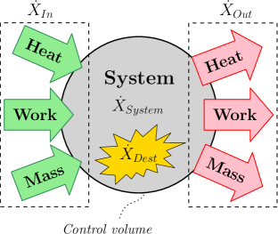
Figure 1: Schematic representation of a system exergy balance defined with respect to a control volume. Exergy fluxes – heat, work, and mass – entering and leaving the control volume are shown.

2.1.1 Exergy Destruction

Any irreversibility in a system, from frictions to chemical reactions, causes entropy increase and, consequently, exergy destruction. In mathematical terms, this is modeled by the following relationship

$$\dot{X}_{Dest}=-T_{0}\cdot\dot{S}_{gen},$$ (3)

where $\dot{S}_{gen}$ is the entropy generation rate. The contribution of exergy destruction is a function of the reference state, which, as already mentioned, must be carefully chosen.

2.1.2 Exergy Transfer

Exergy transfer into ($\dot{X}_{In}$) or out of ($\dot{X}_{Out}$) the system is dependent on three mechanisms: heat, work, and mass.

Component	$\boldsymbol{\dot{X}_{System}}$	$\boldsymbol{\dot{X}_{Heat}}$	$\boldsymbol{\dot{X}_{Work}}$	$\boldsymbol{\dot{X}_{Mass}}$	$\boldsymbol{\dot{X}_{Dest}}$
Longitudinal dynamics (§ 3.2.1)	$\dot{X}_{long}$	$0$	$P_{trac}$	$0$	$-P_{brake}-P_{roll}-P_{aero}$
Electrochemical energy storage device (§ 3.2.2)	$\dot{X}_{batt}$	$\dot{X}_{heat,batt}$	$\dot{W}_{batt}$	$0$	$\dot{X}_{dest,batt}$
Electric motor (§ 3.2.3)	$\dot{X}_{mot}$	$\dot{X}_{heat,mot}$	$\dot{W}_{mot}$	$0$	$\dot{X}_{dest,mot}$
ICE (§ 3.2.4)	$0$	$\dot{X}_{heat,eng}$	$\dot{X}_{work,eng}+\dot{X}_{intk,eng}$	$\dot{X}_{fuel,eng}+\dot{X}_{exh,eng}$	$\dot{X}_{fric,eng}+\dot{X}_{comb,eng}$

Table 1: Exergy balance terms, defined according to Equation (9), for the vehicle’s longitudinal dynamics and its energy storage and conversion devices.

Heat transfer. This term is modeled as the maximum possible work extraction from a Carnot heat engine (i.e., an engine operating between two thermal reservoirs at $T_{0}$ and $T$)

$$\dot{X}_{Heat}=\left(1-\frac{T_{0}}{T}\right)\cdot\dot{Q},$$ (4)

with $\dot{Q}$ the rate of heat exchange and $T$ the temperature of the surface of the system involved in the thermal exchange. The temperature $T$, at which the thermal exchange occurs, is always higher than the reference state temperature $T_{0}$ (see Assumption 1). Therefore, $\dot{Q}$ is always negative and leads to a decrease of exergy within the system.

Work transfer. This quantity is related to a variation of availability due to work ($W$) done on or performed by the system. The general expression is

$$\dot{X}_{Work}=-(\dot{W}-\dot{W}_{Surr})=-(\dot{W}-\mathcal{P}_{0}\dot{\mathcal{V}}),$$ (5)

with $\dot{W}$ the work rate, related to thermomechanical, chemical, or electrical work, and $\dot{W}_{Surr}$ the moving boundary work, function of the reference state pressure and the system volume time derivative $\dot{\mathcal{V}}$. The term $\dot{W}_{Surr}$ is related to the work the system performs with respect to its surroundings. For instance, during an expansion process, the system volume increases and work is performed to “move” the surrounding medium.

We highlight that there is no entropy transfer associated with work. Instead, being exergy a quantification of the availability, work interactions must be considered in the balance equation: when the system is delivering work ($\dot{W}>0$) the exergy decreases, conversely, if the system is experiencing work ($\dot{W}<0$) the exergy increases.

Mass transfer. Exergy can be associated with mass entering or leaving the system. Given a gaseous mixture composed by the chemical species $i$, the variation of exergy with respect to time is expressed as

$$\dot{X}_{Mass}=\sum_{i}\dot{n_{i}}\psi_{i}=\sum_{i}\dot{n}_{i}(\psi_{ph,i}+\psi_{ch,i}),$$ (6)

where, for each species $i$, the exergy variation is given by the exergy flux ($\psi_{i}$) multiplied by the flow rate ($\dot{n}_{i}$) . In particular, $\psi_{i}$ is composed of physical $\psi_{ph,i}$ and chemical $\psi_{ch,i}$ exergies. The physical exergy, modeling the work potential between the current state and the restricted state of the system, is expressed as

$$\psi_{ph,i}=h_{i}-h^{\star}_{i}-T_{0}\cdot(s_{i}-s^{\star}_{i}),$$ (7)

with $h_{i}$ and $h^{\star}_{i}$ the specific enthalpies of the system at the current state and restricted state, respectively, and $s_{i}$ and $s^{\star}_{i}$ the specific entropies of the system at the current state and restricted state. To take into account the different chemical composition between the restricted and reference state, the chemical exergy term is expressed as follows

$$\psi_{ch,i}=\mathcal{R}_{gas}\cdot T_{0}\cdot\log\frac{f^{\star}_{i}}{f_{i,0}},$$ (8)

where $\mathcal{R}_{gas}$ is the ideal gas constant, and $f^{\star}_{i}$ and $f_{i,0}$ are the molar fractions at the restricted and reference state, respectively. Equation (8) is valid only for ideal gases. For further details on the exergy flux, the reader is referred to [18].

2.1.3 Open and Closed Systems

From the concepts introduced in Sections 2.1.1 and 2.1.2, the rate of exergy change for an open system is defined as

$$\begin{split}\dot{X}_{System}=&\overbrace{\left(1-\frac{T_{0}}{T}\right)\cdot\dot{Q}}^{\text{Heat transfer }\dot{X}_{Heat}}\ \overbrace{-(\dot{W}-\dot{W}_{Surr})}^{\text{Work transfer }\dot{X}_{Work}}+\\ &+\underbrace{\sum_{j}\dot{n}_{j}\psi_{j}-\sum_{k}\dot{n}_{k}\psi_{k}}_{\text{Mass transfer }\dot{X}_{Mass}}\ \underbrace{-T_{0}\cdot\dot{S}_{gen}}_{\text{Destruction }\dot{X}_{Dest}}.\end{split}$$ (9)

The exergy associated with the mass transfer is defined starting from Equation (6), considering both the species entering ($i=j$) and exiting ($i=k$) the control volume. The species moving into the control volume lead to an exergy increase. Conversely, the species exiting the control volume lead to an exergy decrease. From Assumption 3 and Equation (5), $\dot{W}_{Surr}$ is equal to zero.

As a reference for the next sections, in Table 1, the exergy balance in Equation (9) is defined for the vehicle’s longitudinal dynamics and its energy storage and conversion devices.

3 Vehicle Model and Exergy Balance

In this section, the modeling of the vehicle longitudinal dynamics, electrochemical energy storage device, electric motor, and ICE is introduced and the exergy balance is carried out relying on the theoretical concepts presented in Section 2 and, in particular, in Table 1. These components are “building blocks” to be used in the description of the overall vehicle architecture, as shown in Section 4.

3.1 Reference State

In this work, the reference state, as defined in Definition 3, is at temperature $T_{0}=298.15K$ and pressure $\mathcal{P}_{0}=1atm$. The atmosphere is assumed to be exclusively composed by four species $k\in\mathcal{K}=\{N_{2},O_{2},H_{2}O,CO_{2}\}$, and other components (mostly argon), combined according to the following molar fractions [19]

$$\begin{split}&f_{N_{2},0}=0.7567,\ f_{O_{2},0}=0.2035,\ f_{CO_{2},0}=0.0003,\\ &f_{H_{2}O,0}=0.0303,\ f_{others,0}=0.0092.\end{split}$$ (10)

3.2 Vehicle Model

The exergy-based modeling framework relates the vehicle’s longitudinal dynamics, the electrochemical storage device, electric motor, and ICE (when used). The transmission is assumed to have zero losses and to transfer all the mechanical power from and to the powertrain. This is in line with [20], in which transmission efficiencies close to 100% are reported.

3.2.1 Longitudinal Dynamics

A vehicle model is based on its longitudinal dynamics. Without loss of generality, in this work the road grade component is neglected. To simplify the notation, time dependency is made explicit only the first time a variable is introduced.

The following balance of forces governs the longitudinal dynamics

$$m_{veh}\cdot\dot{v}(t)=F_{trac}(t)-F_{brake}(t)-F_{roll}(t)-F_{aero}(t),$$ (11)

where $v(t)$ and $\dot{v}$ are the vehicle speed and acceleration, respectively, $m_{veh}$ the vehicle mass, $F_{trac}$ is the traction force at the wheels, and $F_{brake}$, $F_{roll}$, $F_{aero}$ are the braking, rolling friction, and aerodynamic drag forces experienced by the vehicle, respectively. The forces are computed according to the following equations [21]

$$\begin{split}F_{aero}&=\dfrac{1}{2}A_{f}\cdot\rho_{air}\cdot C_{d}\cdot v^{2},\\ F_{roll}&=m_{veh}\cdot g\cdot k_{roll},\\ F_{brake}&=\dfrac{\tau_{brake}}{\mathcal{R}_{wh}},\\ F_{trac}&=\dfrac{P_{trac}(t)}{v(t)},\end{split}$$ (12)

where $P_{trac}$ is the traction power, $\tau_{brake}$ is the braking torque at the wheels, $k_{roll}$ is the rolling friction coefficient, $A_{f}$ is the vehicle frontal area, $C_{d}$ is the aerodynamic drag coefficient, and $\rho_{air}$ is the air density. Note that $P_{trac}$, and consequently $F_{trac}$, is a function of the powertrain architecture. Multiplying both sides of Equation (11) by $v$, the vehicle power balance at the wheels is obtained

$$P_{long}(t) =m_{veh}\cdot\dot{v}\cdot v=\left(F_{trac}-F_{brake}-\right.$$ (13)

$$\left.-F_{roll}-F_{aero}\right)\cdot v=P_{trac}(t)-P_{brake}(t)-$$

$$-P_{roll}(t)-P_{aero}(t),$$

where $P_{brake}$, $P_{roll}$, $P_{aero}$ are the powers associated to $F_{brake}$, $F_{roll}$, and $F_{aero}$, respectively. Recalling that the Hamiltonian of a system is the sum of kinetic and potential energy, Equation (13) can be interpreted as the derivative of the Hamiltonian, i.e., $P_{long}=\dot{H}(t)$. In this particular case, the road grade is assumed to be zero and the potential energy contribution to the Hamiltonian is zero. According to [22], under the assumptions

• no heat flow,

• no exergy flow,

• no mass flow rate,

the following equality holds

$$\dot{X}_{long}(t)=\dot{H}=P_{long},$$ (14)

i.e., the derivative of the Hamiltonian function of the system is equal to its exergy rate, indicated with $\dot{X}_{long}$.

For the electrochemical energy storage device, electric motor, and ICE (used in the HEV), the assumptions listed above do not hold because of heat exchanges with the environment, work, entropy generation, and mass transfer. For these components, the exergy rate balance is not based on the sum of kinetic and potential energy only, thus, it is not equal to the derivative of the Hamiltonian. In the next sections, a careful formulation of the exergy balance for these powertrain components is carried out.

Figure 2: Schematic of the battery cell zero-order model.

3.2.2 Electrochemical Energy Storage Device

An electrochemical energy storage device, in the form of a lithium-ion battery pack, is used in both EV and HEV powertrains. The model is first derived at cell-level and then upscaled to the pack-level.

For the purpose of modeling the losses in the battery cell, a zero-order equivalent circuit model, as the one shown in Fig. 2, is used. From Kirchhoff Voltage Law, the terminal voltage is given by

$$V_{cell}(t)=V_{oc}^{cell}(t)-R_{0}^{cell}\cdot I_{cell}(t),$$ (15)

where $V_{oc}^{cell}$ is the cell open circuit voltage, $R_{0}^{cell}$ is the lumped internal resistance, and $I_{cell}$ is the battery cell current. The convention for $I_{cell}$ is as follows

$$\begin{split}&\begin{array}[]{c}\begin{cases}I_{cell}\leq 0&\textrm{if the battery is charging},\\ I_{cell}>0&\textrm{otherwise}.\end{cases}\end{array}\end{split}$$ (16)

The battery State of Charge ($SoC$) dynamics is defined as

$$\dot{SoC}(t)=-\frac{I_{cell}}{3600\cdot Q_{nom}^{cell}},$$ (17)

where $Q_{nom}^{cell}$ is the battery cell nominal capacity in $Ah$. From the cell nominal voltage $V_{nom}^{cell}$, the device nominal energy is obtained as

$$E_{nom}^{cell}=V_{nom}^{cell}\cdot Q_{nom}^{cell}\cdot 3600.$$ (18)

From the battery cell power $P_{cell}(t)=V_{cell}\cdot I_{cell}$, the State of Energy ($SoE$) dynamics is defined as

$$\dot{SoE}(t)=-\dfrac{P_{cell}}{E_{nom}^{cell}}.$$ (19)

The cell internal resistance $R_{0}^{cell}$ and the open circuit voltage $V_{oc}^{cell}$ as a function of $SoC$ are shown in Fig. 3. These data have been collected at the Stanford Energy Control Lab from a LG Chem INR21700-M50 NMC cylindrical cell with nominal capacity $Q_{nom}^{cell}=4.85Ah$. The internal resistance is identified according to the procedure described in [23] with data from [24], namely, the cell is discharged through the current pulse train shown in Fig. 4. Then, the voltage drop $\Delta V_{cell}$, after each pulse, is evaluated and divided by the measured current $I_{cell}$ to obtain the cell internal resistance at different $SoC$.

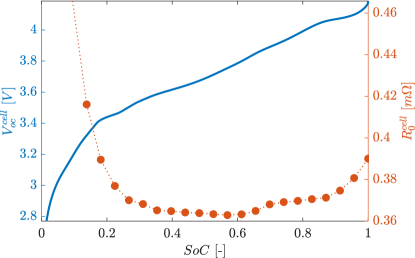
Figure 3: Battery cell open circuit voltage and internal resistance as a function of $SoC$ at $298K$.

The battery cell temperature $T_{cell}(t)$ and heat transfer with the environment play a relevant role in the evaluation of the exergy balance shown later. Thus, the following lumped thermal model is introduced

$$\mathrm{C}_{cell}\cdot\dot{T}_{cell}=(V_{oc}^{cell}-V_{cell})\cdot I_{cell}+\dot{Q}_{cell}(t),$$ (20)

where $\mathrm{C}_{cell}$ is the battery cell thermal capacity, the first term on the right-hand-side is the heat generation due to Joule losses, and $\dot{Q}_{cell}$ is the heat transfer between the device and the environment, defined as

$$\dot{Q}_{cell}=\mathrm{h}_{out,cell}\cdot(T_{0}-T_{cell}),$$ (21)

with $\mathrm{h}_{out,cell}$ the thermal transfer coefficient between the battery cell and the environment, at the reference temperature $T_{0}$. The cell thermal capacity ($\mathrm{C}_{cell}$) and thermal transfer coefficient ($\mathrm{h}_{out,cell}$) are identified using the current pulse train discharge test shown in Fig. 4. In particular, the identification is performed minimizing the Root Mean Square Error (RMSE) between the cell experimental temperature (measured by a thermocouple) and the simulated one. Fig. 5 shows a comparison between measured and simulated temperature profiles. In this context, a RMSE of $0.114K$ is obtained.

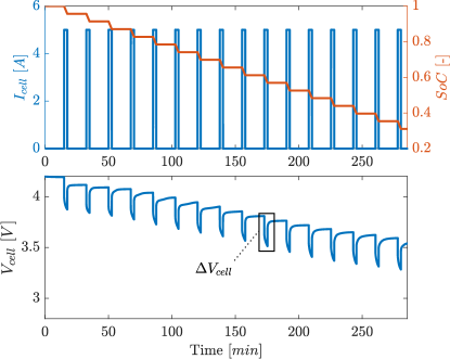
Figure 4: Current pulse train discharge test and corresponding $SoC$ and terminal voltage $V_{cell}$. The voltage drop $\Delta V_{cell}$ at 0.6 $SoC$ is highlighted.

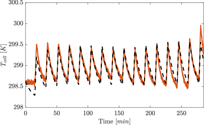
Figure 5: Comparison between the experimental and simulated temperature profile during the current pulse train discharge test of Fig. 4.

From the cell-level modeling, electrical and thermal quantities are upscaled to the pack-level as

$$\begin{split}&R_{0}\left(SoC\right)=\frac{N_{s}}{N_{p}}R_{0}^{cell}\left(SoC\right),\\ &V_{oc}\left(SoC\right)=N_{s}\cdot V_{oc}^{cell}\left(SoC\right),\\ &V_{nom}=N_{s}\cdot V_{nom}^{cell},\\ &Q_{nom}=N_{p}\cdot Q_{nom}^{cell},\\ &E_{nom}=V_{nom}\cdot Q_{nom}\cdot 3600,\\ &\mathrm{C}_{batt}=N_{s}\cdot N_{p}\cdot\mathrm{C}_{cell},\\ &\mathrm{h}_{out,batt}=N_{s}\cdot N_{p}\cdot\mathrm{h}_{out,cell},\end{split}$$ (22)

with $N_{s}$ and $N_{p}$ the number of cells in series and parallel configuration. Given the parameters in Equation (22), Equations (15), (17), (19), (20), and (21) are rewritten as

$$\begin{split}&V_{batt}(t)=V_{oc}(t)-R_{0}\cdot I_{batt}(t),\\ &\dot{SoC}=-\frac{I_{batt}}{3600\cdot Q_{nom}},\\ &\dot{SoE}=-\dfrac{P_{batt}(t)}{E_{nom}}=-\dfrac{V_{batt}\cdot I_{batt}}{E_{nom}},\\ &\mathrm{C}_{batt}\cdot\dot{T}_{batt}(t)=\ (V_{oc}-V_{batt})\cdot I_{batt}+\dot{Q}_{batt}(t),\\ &\dot{Q}_{batt}=\mathrm{h}_{out,batt}\cdot(T_{0}-T_{batt}).\end{split}$$ (23)

The battery pack is assumed to be a closed system, as no mass is exchanged between the device and the environment. Thus, according to [1], Equation (9) can be written as

$$\dot{X}_{batt}(t)=\dot{X}_{heat,batt}(t)+\dot{W}_{batt}(t)+\dot{X}_{dest,batt}(t),$$ (24)

where $\dot{X}_{batt}$ is the battery exergy rate, $\dot{W}_{batt}=-P_{batt}$ is the work rate to/from the battery and $\dot{X}_{dest,batt}=-T_{0}\dot{S}_{gen,batt}(t)$ is the exergy destruction within the battery, where $\dot{S}_{gen,batt}$ is in turn the entropy generation rate. $\dot{X}_{heat,batt}$ is the exergy transfer contribution due to heat transfer computed as in Equation (4)

$$\dot{X}_{heat,batt}=\left(1-\dfrac{T_{0}}{T_{batt}}\right)\cdot\dot{Q}_{batt}.$$ (25)

The entropy generation rate is computed formulating the entropy balance for the battery ($\dot{S}_{batt}$), while recalling the closed system assumption [1]. In this scenario, the entropy variation is due to the heat transferred to or from the system and the entropy generation

$$\dot{S}_{batt}(t)=\dot{S}_{gen,batt}+\dot{S}_{in,batt}(t)-\dot{S}_{out,batt}(t).$$ (26)

Given that $T_{batt}\geq T_{0},\ \forall t$, then $\dot{S}_{in,batt}=0$ (i.e., the entropy transfer rate from the environment to the battery is zero), since the heat is always going from the device to the environment. On the other hand, the entropy transfer rate from the battery to the environment is obtained as

$$-\dot{S}_{out,heat}=\dfrac{\dot{Q}_{batt}}{T_{batt}}=\dfrac{\mathrm{h}_{out,batt}\cdot\left(T_{0}-T_{batt}\right)}{T_{batt}}.$$ (27)

According to [25], the entropy for a closed system is a function of its states

$$S_{batt}=S_{batt}\left(T_{batt},\mathcal{P}_{batt}(t)\right),$$ (28)

where $\mathcal{P}_{batt}$ is the battery pressure. Recalling that the system is incompressible (Assumption 3), the pressure dependence of Equation (28) can be removed, leading to entropy generation and transfer due to heat exchange only. Given Definition 1, the following relationship hold

$$dS_{batt}=\dfrac{\mathrm{C}_{batt}\cdot dT_{batt}}{T_{batt}},$$ (29)

and, dividing both sides of Equation (29) by $dt$, Equation (26) is rewritten as

$$\dot{S}_{batt}=\dfrac{\mathrm{C}_{batt}}{T_{batt}}\cdot\dot{T}_{batt}.$$ (30)

Recalling Equations (23), (26), (27), and (29), the final expression for the entropy generation rate is retrieved

$$\dot{S}_{gen,batt}=\dfrac{\left(V_{oc}-V_{batt}\right)\cdot I_{batt}}{T_{batt}}=\frac{R_{0}\cdot I_{batt}^{2}}{T_{batt}},$$ (31)

which is always positive, coherently with the second law of thermodynamics.

Finally, the battery exergy balance is obtained substituting Equations (25) and (31) into Equation (24)

$$\begin{split}\dot{X}_{batt}&=\left(1-\frac{T_{0}}{T_{batt}}\right)\cdot\dot{Q}_{batt}-P_{batt}-\\ &\hskip 10.00002pt-\frac{T_{0}}{T_{batt}}R_{0}\cdot I_{batt}^{2}.\end{split}$$ (32)

3.2.3 Electric Motor

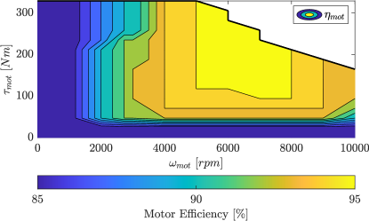
(a) Electric Vehicle.

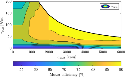
(b) Hybrid Electric Vehicle.

Figure 6: Motor efficiency maps for EV and HEV.

Electric motors are energy conversion devices working either in motoring (i.e., torque is provided to the wheels) or in generating (i.e., torque is received from the wheels) mode. For the purpose of this work, the actuator is modeled using static efficiency maps $\eta_{mot}(\tau_{mot},\omega_{mot})$, function of the motor torque ($\tau_{mot}$) and speed ($\omega_{mot}$). The static maps used in this work, for the EV and HEV case studies, are shown in Fig. 6. The motor torque is in turn obtained as

$$\tau_{mot}=\textrm{min}\left(\left|\frac{P_{mot}(t)}{\omega_{mot}}\right|,\tau_{max,mot}\right),$$ (33)

where $\tau_{max,mot}$ is the maximum torque that the motor can deliver, and the motor power, $P_{mot}$, is computed as

$$P_{mot}=P_{batt}\cdot\eta^{\mathrm{sign}(I_{batt})}_{mot},$$ (34)

with the $\mathrm{sign}$ function defined as:

$$\mathrm{sign}(I_{batt})=\begin{array}[]{c}\begin{cases}-1\ &\text{if}\ I_{batt}<0,\\ 0\ &\text{if}\ I_{batt}=0,\\ 1\ &\text{if}\ I_{batt}>0.\end{cases}\end{array}$$ (35)

Following the same reasoning of the battery, a thermal model for the motor is introduced. The thermal model, as well as its parameters, are borrowed from [26]. This reference provides data for Interior Permanent Magnet Synchronous Machines (IPMSMs), commonly used devices in both EVs and HEVs [27]. The model describes the temperature evolution of both copper windings and stator iron. The heat generation within the rotor is considered negligible and the motor is assumed to directly exchange heat with the environment (no coolant is considered). The model is characterized by two heat capacities $\mathrm{C}_{mot,copper}$ and $\mathrm{C}_{mot,iron}$, as well as by two thermal transfer coefficients $\mathrm{h}_{mot,copper}$ and $\mathrm{h}_{mot,iron}$, for copper and iron, respectively. These coefficients are combined as follows

$$\begin{split}&\mathrm{C}_{mot}=\alpha\cdot\mathrm{C}_{mot,copper}+\beta\cdot\mathrm{C}_{mot,iron},\\ &\mathrm{h}_{out,mot}=\alpha\cdot\mathrm{h}_{mot,copper}+\beta\cdot\mathrm{h}_{mot,iron},\end{split}$$ (36)

where $\alpha$ and $\beta$ represent the copper and iron mass fractions in the device, set to $0.15$ and $0.85$ [28], respectively. The motor losses account for Joule effect (in the copper phase), iron hysteresis, and friction

where $I_{d}$ and $I_{q}$ are the $d$ and $q$ axes currents, $L_{d}$ and $L_{q}$ are the $d$ and $q$ axes inductances, $k_{h}$ and $k_{f}$ are experimentally obtained parameters used to compute the motor iron and friction losses, and $\Lambda_{pm}$ is defined as $\sqrt{3/2}\cdot\lambda_{pm}$ (with $\lambda_{pm}$ the permanent magnet flux linkage). $R_{s}$ is the stator resistance, function of the motor temperature $T_{mot}$

$$R_{s}=R_{s,0}\cdot\left[1+\xi\cdot\left(T_{mot}-T_{0}\right)\right],$$ (38)

where $R_{s,0}$ is the stator resistance at $T_{0}$ and $\xi$ is an identified parameter modeling the temperature dependence. The computation of $I_{d}$ and $I_{q}$ would require the simulation of the low level electrical dynamics and controls of the motor. Since this is out of the scope of the work, a simplified procedure for the computation of these currents is exploited. We assume the motor to be controlled by a maximum torque per ampere (MTPA) algorithm, which, as described in [29], provides the $I_{d,ref}$ and $I_{q,ref}$ reference currents to the low level controller. Then, assuming the reference currents to be perfectly tracked, the following holds

$$I_{d}=I_{d,ref},\quad I_{q}=I_{q,ref}.$$ (39)

Overall, the electric motor thermal model reads

$$\begin{split}&\mathrm{C}_{mot}\cdot\dot{T}_{mot}=\mathrm{h}_{out,mot}\cdot\left(T_{0}-T_{mot}\right)+P_{mot,fric}+\\ &+P_{mot,copper}+P_{mot,iron}.\end{split}$$ (40)

Similarly to the battery pack, the electric motor is a closed and incompressible system and the exergy balance is written as

$$\dot{X}_{mot}(t)=\dot{X}_{heat,mot}(t)+\dot{W}_{mot}(t)+\dot{X}_{dest,mot}(t),$$ (41)

where $\dot{X}_{mot}$ is the rate of exergy change in the motor and $\dot{X}_{heat,mot}$ is the exergy transfer rate due to heat, computed as

$$\dot{X}_{heat,mot}=\left(1-\dfrac{T_{0}}{T_{mot}}\right)\cdot\dot{Q}_{mot}(t),$$ (42)

with $\dot{Q}_{mot}=\mathrm{h}_{out,mot}\cdot(T_{0}-T_{mot})$ the heat exchange between the motor and the environment. $\dot{W}_{mot}$ is the work rate related to the motor, which is equal to zero. This is reasonable because both the works at the input and output of the motor are already taken into account in other components of the powertrain: the work in input to the motor is the battery power $P_{batt}$, and the work in output from the motor is the traction power $P_{trac}$ of the longitudinal dynamics model (as defined in Section 3.2.1).

The term $\dot{X}_{dest,mot}=-T_{0}\cdot\dot{S}_{gen,mot}(t)$ is the rate of exergy destruction within the motor, and $\dot{S}_{gen,mot}$ is the related entropy generation computed according to the procedure shown for the battery (see Equation (26)). Assuming the electric motor to be incompressible and with constant heat capacity, the following balance is obtained

$$\begin{split}\dot{S}_{mot}(t)=&\ \dot{S}_{gen,mot}+\dot{S}_{in,mot}(t)-\dot{S}_{out,mot}(t),\end{split}$$ (43)

where $\dot{S}_{mot}(t)$ is the motor entropy rate, and $\dot{S}_{in,mot}$ and $\dot{S}_{out,mot}$ are the entropy transfer into or out of the motor, respectively. The last term on the right-hand-side of Equation (43) is computed as

$$-\dot{S}_{out,mot}=\dfrac{\dot{Q}_{mot}}{T_{mot}}=\mathrm{h}_{out,mot}\cdot\dfrac{T_{0}-T_{mot}}{T_{mot}}.$$ (44)

$\dot{S}_{in,mot}$ is equal to zero because $T_{mot}>T_{0},\ \forall t$. Moreover, following the same procedure showed in Equations (29) and (30), the motor entropy rate reads as

$$\dot{S}_{mot}=\dfrac{\mathrm{C}_{mot}\cdot{\dot{T}_{mot}}}{T_{mot}},$$ (45)

and the motor entropy generation is obtained combining Equations (43), (44), and (45)

$$\dot{S}_{gen,mot}=\dfrac{P_{mot,copper}+P_{mot,iron}+P_{mot,fric}}{T_{mot}}.$$ (46)

Finally, the motor exergy balance is obtained substituting Equations (42) and (46) into Equation (41) as

$$\begin{split}\dot{X}_{mot}&=\left(1-\frac{T_{0}}{T_{mot}}\right)\cdot\dot{Q}_{mot}-\\ &\hskip 10.00002pt-\frac{T_{0}\cdot(P_{mot,copper}+P_{mot,iron}+P_{mot,fric})}{T_{mot}}.\end{split}$$ (47)

3.2.4 Internal Combustion Engine

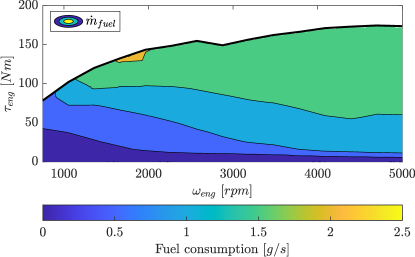
Figure 7: ICE fuel consumption map used in this work.

In this work, an inline $4$-cylinder gasoline engine is considered for use in the HEV architecture. Starting from [17], the steady-state exergy balance for the ICE is written as follows

$$\begin{split}&\dot{X}_{fuel,eng}(t)+\dot{X}_{intk,eng}(t)=-\left[\dot{X}_{work,eng}(t)+\right.\\ &\left.\dot{X}_{exh,eng}(t)+\dot{X}_{heat,eng}(t)+\dot{X}_{fric,eng}(t)+\right.\\ &\left.+\dot{X}_{comb,eng}(t)\right],\end{split}$$ (48)

where $\dot{X}_{fuel,eng}$ is the fuel availability, computed according to [30]

with $X_{spec,fuel}$ the specific fuel chemical exergy, $x$ and $y$ known from the fuel chemical formula $C_{x}H_{y}$ (e.g., for gasoline $x=8$, $y=18$), and $LHV$ the fuel lower heating value. The fuel consumption $\dot{m}_{fuel}$ is retrieved from the map in Fig. 7, function of $\omega_{eng}$ – the engine rotational speed – and $\tau_{eng}$ – the engine torque –. When the tank is completely filled, the maximum fuel availability is computed as

$$X_{fuel,max}=\mathcal{V}_{tank}\cdot\rho_{fuel}\cdot X_{spec,fuel},$$ (50)

where $\mathcal{V}_{tank}$ is the tank volume and $\rho_{fuel}$ is the fuel density. $\dot{X}_{intk,eng}$ is the intake exergy flow, related to the air entering the engine for combustion, and, according to Equation (9), takes the following form

$$\dot{X}_{intk,eng}=\sum_{j\in\mathcal{K}}\dot{n}_{intk,j}(t)\cdot\psi_{j}(t).$$ (51)

where $\dot{n}_{intk,j}$ is the molar flow rate of a species $j$ in the intake manifold and $\psi_{j}$ is the exergy flux. This term accounts for less than 1% of the fuel availability and can be neglected [31]: $\dot{X}_{intk,eng}=0$.

The term $\dot{X}_{exh,eng}$ models the exergy exchanged with the environment through the exhaust gas. According to Section 2, this term is function of the species $k$ composing the exhaust gas, namely, $N_{2}$, $O_{2}$, $H_{2}O$, and $CO_{2}$, and is defined as

$$\begin{split}\dot{X}_{exh,eng}&=-\sum_{k\in\mathcal{K}}\dot{n}_{exh,k}(t)\cdot\psi_{k}(t)=\\ &=-\sum_{k\in\mathcal{K}}\dot{n}_{exh,k}\cdot\left(\psi_{ch,k}(t)+\psi_{ph,k}(t)\right),\end{split}$$ (52)

where $\dot{n}_{exh,k}$ is the molar flow rate of a species $k$ in the exhaust manifold and $\psi_{ch,k}$ and $\psi_{ph,k}$ are the specific chemical and physical exergies defined in Section 2. To describe the combustion process and compute Equation (52), we exploit the mean-value approach, in which the combustion process is not analyzed cycle by cycle (i.e., in the crank-angle domain), but averaged, over time, for the four cylinders. This is a reasonable approach since the goal of this work is the exergetic characterization of the ICE and not the optimization of the combustion process variables, such as spark, injection, and valve timings. Assuming the engine is working at stoichiometric conditions, all the oxygen is burnt during combustion according to the following reaction [33]

$$\begin{split}&C_{8}H_{18}+z_{comb}\left(O_{2}+3.76N_{2}\right)\rightarrow\\ &a_{comb}CO_{2}+b_{comb}H_{2}O+c_{comb}N_{2},\end{split}$$ (53)

where $a_{comb}=x$, $b_{comb}=y/2$, $z_{comb}=a_{comb}+b_{comb}/2$ and $c_{comb}=3.76z_{comb}$. The stoichiometric assumption is realistic for a spark-ignition engine and ensures the optimal operation of the three-way catalyst [33]. Starting from the fuel mass flow rate, $\dot{m}_{fuel}$, known for a given engine operating point, the air mass flow rate is

$$\dot{m}_{air}(t)=\dot{m}_{fuel}\cdot AFR_{stoich},$$ (54)

with $AFR_{stoich}$ the stoichiometric air-fuel ratio. In accordance with [30], the exhaust gas mass flow rate is computed as $\dot{m}_{exh}(t)=\dot{m}_{fuel}+\dot{m}_{air}$ and the corresponding molar flow rate reads as

$$\dot{n}_{exh}(t)=\dfrac{\dot{m}_{exh}}{\sum_{k\in\mathcal{K}}f^{\star}_{exh,k}\cdot M_{k}},$$ (55)

where $M_{k}$ is the molar mass for the $k$-th species in the exhaust manifold. Starting from Equation (55), the contribution of the different exhaust gas species to $\dot{n}_{exh}$ is given by

$$\dot{n}_{exh,k}(t)=\dot{n}_{exh}\cdot f^{\star}_{exh,k},$$ (56)

where $f^{\star}_{exh,k}$ is the molar fraction of the species $k$ at the restricted state

$$\begin{split}&f^{\star}_{exh,CO_{2}}=\dfrac{a_{comb}}{n_{exh,tot}},\ f^{\star}_{exh,H_{2}O}=\dfrac{b_{comb}}{n_{exh,tot}},\\ &f^{\star}_{exh,N_{2}}=\dfrac{c_{comb}}{n_{exh,tot}},\ f^{\star}_{exh,O_{2}}=0,\end{split}$$ (57)

with $n_{exh,tot}=a_{comb}+b_{comb}+c_{comb}$ the number of moles of the products, from the right hand side of Equation (53). The chemical exergy is obtained similarly to Equation (8)

$$\psi_{ch,k}=\mathcal{R}_{gas}\cdot T_{0}\cdot\log\left(\dfrac{f^{\star}_{exh,k}}{f_{k,0}}\right).$$ (58)

Recalling Equation (7), the physical exergy is

$$\psi_{ph,k}=h_{k}-h_{k}^{\star}-T_{0}\cdot(s_{k}-s_{k}^{\star}),$$ (59)

where $h_{k}$ and $h^{\star}_{k}$ are the specific enthalpies of a species $k$ in the exhaust manifold and at the restricted state, respectively. Similarly, $s_{k}$ and $s^{\star}_{k}$ are the specific entropies in the exhaust manifold and at the restricted state. To compute the thermodynamic properties of the gaseous species (enthalpy and entropy), the experimentally fitted NASA polynomials [34], function of the exhaust gas mixture temperature, are used.

The exergy transfer related to the mechanical work generation ($\dot{X}_{work,eng}$) is obtained as follows

$$\dot{X}_{work,eng}=-P_{eng}(t)=-\tau_{eng}(t)\cdot\omega_{eng}(t).$$ (62)

In accordance with Equation(4), the availability change related to heat transfer towards the cylinder walls is modeled as

$$\dot{X}_{heat,eng}=\left(1-\dfrac{T_{0}}{T_{eng}}\right)\cdot\dot{Q}_{eng}(t),$$ (63)

where $\dot{Q}_{eng}$ is the thermal exchange between the in-cylinder mixture, at temperature $T_{eng}$, and the cylinder walls. Relying on the time-averaged Taylor&Toong correlation [35], the heat transfer $\dot{Q}_{eng}$ is computed as follows

where $k_{g}$ is the mixture conductivity, $\mu_{g}$ the mixture viscosity, $B$ the cylinder bore, $T_{c}$ the coolant temperature, and $a$ and $b$ empirical, dimensionless, coefficients function of the engine characteristics: $a$ is tuned in order to reach a contribution of $\dot{X}_{heat,eng}$ to the balance in Equation (48) of around $10\%$ (in line with [16]). $T_{eng}$, $k_{g}$, and $\mu_{g}$ are function of the air-fuel ratio which, in this work, is constant and equal to the stoichiometric value $AFR_{stoich}$. Therefore, $T_{eng}$, $k_{g}$, and $\mu_{g}$ are also constant and determined relying on data available in [33] for spark-ignition engines.

Finally, the combustion irreversibility term, the principal source of loss in the ICE [36, 17], is obtained inverting Equation (48)

$$\begin{split}\dot{X}_{comb,eng}=&-\dot{X}_{fuel,eng}-\dot{X}_{work,eng}-\\ &-\dot{X}_{exh,eng}-\dot{X}_{heat,eng}-\\ &-\dot{X}_{fric,eng}.\end{split}$$ (65)

with $\dot{X}_{fric,eng}$ the friction exergy loss computed numerically. Through Equation (65), one avoids to compute the complex governing combustion reactions. Finally, substituting Equations (52), (62), (63), (65), into Equation (48), the engine exergy balance can be obtained.

3.3 Vehicle Exergy Balance

Combining the exergy rate expressions derived for the electrochemical storage device (Section 3.2.2), the electric motor (Section 3.2.3), the ICE (Section 3.2.4), and the vehicle longitudinal dynamics (Section 3.2.1), the overall exergy balance for EVs and HEVs is derived and reported in Equations (60) and (61), respectively. The formulation of the longitudinal dynamics term, $\dot{X}_{long}$, is the same for both architectures, with the traction power at the wheels computed either as

$$P^{EV}_{trac}=P_{mot}\cdot\eta_{diff}^{\mathrm{sign}(I_{batt})},$$ (66)

or

$$P^{HEV}_{trac}=(P_{mot}+P_{eng})\cdot\eta_{diff}^{\mathrm{sign}(I_{batt})},$$ (67)

whether the vehicle is an EV or HEV. In particular, for the EV case, the balance in Equation (60) is given by summing to $\dot{X}_{long}$ the battery and electric motor exergy rates. In this context, two identical electric motors are used and the corresponding exergy term is multiplied by a factor of two. A similar procedure is followed for the HEV, where $\dot{X}_{veh}^{HEV}$ is obtained including also the ICE (Equation (61)). Therefore, the rates are integrated over the length of the driving cycle, $t_{f}$, and a quantification of the powertrain exergy is obtained. In Equations (60) and (61), the term $X_{batt}(0)$ is the exergy stored in the battery at the beginning of a driving cycle, function of the initial $SoC$ and of the battery pack nominal energy $E_{nom}$

$$X_{batt}(0)=SoC(0)\cdot E_{nom}.$$ (68)

In Equation (61), the term $X_{fuel,max}$ represents the exergy initially stored in the fuel tank (defined in Equation (50)). To facilitate the reading, Equations (60) and (61) are color-coded. Light-blue, orange, green, and magenta are used for the exergy terms associated with the longitudinal dynamics, battery, electric motor, and ICE, respectively.

In the balances $\dot{X}_{veh}^{EV}$ and $\dot{X}_{veh}^{HEV}$, $\dot{X}_{batt}$ represents a storage feature describing the way the stored exergy is exchanged with the environment ($\dot{X}_{heat,batt}$), transformed into useful work ($P_{batt}$), or destroyed ($\dot{X}_{dest,batt}$). On the other hand, $\dot{X}_{long}$ and $\dot{X}_{mot}$ describe how exergy is transferred to the wheels ($P_{trac}$), destroyed ($P_{aero}$, $P_{roll}$, $P_{brake}$, or $\dot{X}_{dest,mot}$), or exchanged with the environment ($\dot{X}_{heat,mot}$). In the case of the HEV, $\dot{X}_{fuel,eng}$ is the exergy stored in the fuel, which is then transformed into useful work ($\dot{X}_{work,eng}$), destroyed (e.g., through $\dot{X}_{comb,eng}$), and exchanged with the environment (e.g., through $\dot{X}_{heat,eng}$).

As soon as the vehicle starts moving, the exergy flows from the energy sources to the wheels and is lost due to transfer and destruction phenomena. The vehicle exergy can never increase over a driving cycle, it can only be destroyed, lost to the environment, or used to propel the vehicle. To exploit this concept, the following normalized quantities are defined

$$\begin{split}X^{EV}_{rel}&=\dfrac{X^{EV}_{veh}}{X_{batt,max}},\\ X^{HEV}_{rel}&=\dfrac{X^{HEV}_{veh}}{X_{batt,max}+X_{fuel,max}},\end{split}$$ (69)

where $X_{batt,max}=E_{nom}$ and, as shown in Equations (60) and (61), $X^{EV}_{veh}$ and $X^{HEV}_{veh}$ are the EV and HEV exergy states, respectively. For the EV case, $X^{EV}_{rel}=1$ corresponds to the maximum available work, i.e., to the fully charged battery. On the other hand, in the HEV the availability is maximized when the battery pack is fully charged and the tank is filled to its maximum capacity: this condition corresponds to $X^{HEV}_{rel}=1$.

The net amount of exergy lost in the powertrain due to the conversion of the electrical (from the battery) and mechanical (from the ICE) power into traction power is referred to as $E_{loss,pwt}$ and takes the following form

$$\begin{split}E^{EV}_{loss,pwt}&=E_{trac}^{EV}-E_{batt},\\ E^{HEV}_{loss,pwt}&=E_{trac}^{HEV}-E_{batt}+X_{work,eng},\end{split}$$ (70)

for the EV and HEV case, respectively. In Equation (70), $E_{trac}^{EV}$, $E_{trac}^{HEV}$, and $E_{batt}$ are obtained integrating the corresponding quantities $P_{trac}^{EV}$, $P_{trac}^{HEV}$, and $P_{batt}$ over the duration of the driving cycle.

4 Case Studies

The proposed framework is tested on an EV and a parallel HEV characterized by the parameters listed in Table 2. The EV is equipped with two electric motors (with efficiency map in Fig. 6a) and a battery pack with nominal energy $E_{nom}=90kWh$. The HEV has one electric motor (with efficiency map in Fig. 6b), a battery pack with nominal energy $E_{nom}=1kWh$, and a spark-ignition ICE characterized by the fuel consumption map in Fig. 7. A schematic representation of the two architectures is provided in Fig. 8.

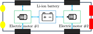
(a) Electric Vehicle.

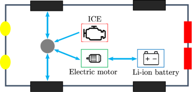
(b) Hybrid Electric Vehicle.

Figure 8: Schematic representation of the powertrain architectures.

The simulators are borrowed from the MathWorks Powertrain Blockset toolbox [37], in which forward models for both EVs and HEVs are provided. The driving cycle is the driver’s desired speed, which is followed relying on the battery (for the EV) or on a combination of battery and ICE for the HEV case study (a tracking error lower than $1km/h$ is ensured). The Matlab model is enhanced with the battery, electric motor, and ICE thermal models – described in Equations (23), (40), and (64) – and the corresponding exergy balances – formalized in Equations (32), (47), and (48) –.

Simulations are carried out considering the World harmonized Light-duty vehicles Test Procedure (WLTP), featuring a mix of urban and highway driving conditions [38], and the reference state defined in Section 3.1.

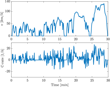
(a) Speed and C-rate profiles for the EV.

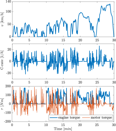
(b) Speed, C-rate, and electric motor/engine torques for the HEV.

Figure 9: Simulation results for the EV and HEV along the WLTP driving cycle.

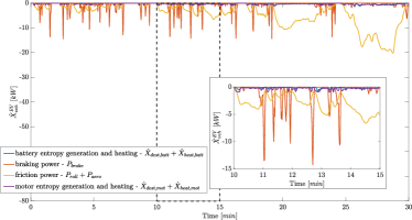
(a) Electric Vehicle.

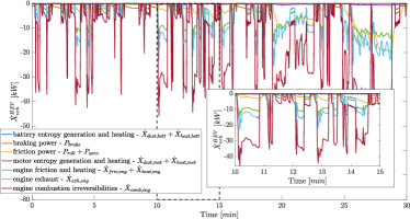
(b) Hybrid Electric Vehicle.

Figure 10: Exergy rate terms $\dot{X}$ and $P$ over the WLTP driving cycle. In the EV case study, the zoomed portion highlight that friction and braking terms are dominating the balance. In the HEV case, the engine related quantities are the principal source of availability loss.

4.1 Results

For both the EV and HEV, the vehicle speed and the corresponding C-rate profiles are shown in Fig. 9. In Fig. 9b, the torque split between ICE and electric motor, computed by the energy management strategy, is shown. The management strategy, already implemented in the HEV simulator, is based on the Equivalent Consumption Minimization Strategy (ECMS) [21]. This is a Pontryagin’s minimum principle-based algorithm that optimizes the power split between the battery pack and the ICE, minimizing the fuel consumption.

To assess the exergetic behavior of the vehicle, the evolution of the exergy rate terms in $\dot{X}_{veh}^{EV}$ and $\dot{X}_{veh}^{HEV}$ is shown in Fig. 10. The EV simulation results highlight that most of the available work is lost due to friction and braking (Fig. 10a). Moreover, a non-negligible portion of the losses is due to battery and motor heating, and entropy generation. In the HEV case, Fig. 10b shows that the drivetrain friction losses are overcame by the engine irreversibilities and exergy transfer to the environment (through the exhaust gas). In this context, the battery and motor losses are, in practice, negligible.

Integrating the exergy rate quantities in Fig. 10, the exergy transfer and destruction terms are obtained. The contribution of each term is expressed as a percentage of the total losses experienced along the driving cycle and computed as $X^{EV}_{veh}(t_{f})-X^{EV}_{veh}(0)$ and $X^{HEV}_{veh}(t_{f})-X^{HEV}_{veh}(0)$ for the EV and HEV, respectively. In the EV case study (Fig. 11a), the electric motor exergy losses account for $5\%$ of the total, while the battery accounts for ~$1\%$. As shown in Fig. 11a, most of the losses are due to rolling friction, aerodynamic drag, and $E_{loss,pwt}^{EV}$. This is in line with the fact that efficiencies of energy storage/conversion devices in electric powertrains are generally around $90\%$ [21]. A key advantage of the proposed exergy-based modeling is the possibility to distinguish between the different sources of irreversibility, e.g., between Joule losses in battery and electric motor. This provides fundamental information to assess, at vehicle and powertrain-leve, how inefficiency is spread. In the HEV case study, losses related to the battery and electric motor are almost negligible, being as small as the $1\%$ of the total (see Fig. 11b). The primary loss term is the availability destruction in the ICE due to combustion reactions (~$47\%$ of the total). $X_{comb,eng}$ is mainly related to the difference in chemical potential between the reactants and products participating in the combustion reaction. Moreover, this term – obtained from Equation (65) – lumps together the unmodeled exergy contributions given by blow-by gases, unburnt fuel, and intake air flow (overall, these terms account for ~$5\%$ of the total balance [17]). The contribution of the combustion irreversibilities is also related to the fraction of fuel which can be converted into useful, braking, work: the higher the efficiency, the lower $X_{comb,eng}$. Considering the fuel consumption map in Fig. 7, the ICE average efficiency is $28\%$ (computed along the driving cycle), meaning that only a small portion of the fuel thermal energy is used to fulfill the traction power $P^{HEV}_{trac}$. Together, the losses associated to the ICE account for more than $80\%$. This is expected as the ICE is rather an inefficient component in which, according to [18] and depending on the operating conditions, only at most the $30$-$35\%$ of the fuel availability can be converted into braking work.

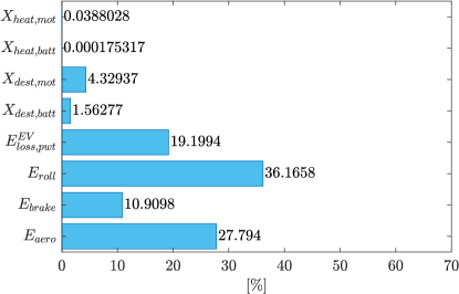
(a) Electric Vehicle.

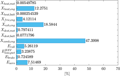
(b) Hybrid Electric Vehicle.

Figure 11: Vehicle exergy losses over the WLTP driving cycle. The contribution of each term is expressed as a percentage of the total losses experienced along the driving cycle. In the EV case, rolling friction, aerodynamic drag, and $E_{loss,pwt}^{EV}$ are dominating. In the HEV scenario, the combustion irreversibilities term $X_{comb,eng}$ has the highest impact on the total balance.

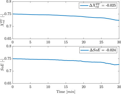
(a) Electric Vehicle.

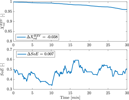
(b) Hybrid Electric Vehicle.

Figure 12: Relative exergies $X_{rel}^{EV}$ and $X_{rel}^{HEV}$ and battery $SoE$ profiles over the WLTP driving cycle.

In Fig. 12, the relative exergy quantities $X_{rel}^{EV}$ and $X_{rel}^{HEV}$, defined in Equation (69), are computed and compared to the $SoE$. For what concerns the EV (Fig. 12a), at the beginning of the driving cycle the battery pack is charged to $SoE=0.75$. The evolution of the $SoE$ and $X_{rel}^{EV}$ is similar: this is expected since the battery is the only storage device and its charged capacity defines the maximum availability of the system. Computing the difference between the initial (at $0s$) and final (at $t_{f}$) state of $SoE$ and $X_{rel}^{EV}$ leads to $\Delta SoE=-0.024$ and $\Delta X_{rel}^{EV}=-0.025$, respectively. The lower value of $\Delta X_{rel}^{EV}$ with respect to $\Delta SoE$ is due to the exergy balance formulation which, according to Equation (61), takes into account also the losses due to entropy generation and heat transfer. The discrepancy between $\Delta X_{rel}^{EV}$ and $\Delta SoE$ proves the ability of the exergy-based modeling in quantifying the availability loss not just as a function of the electrical work $P_{batt}\cdot I_{batt}$ but also of the interaction with the surroundings (heat transfer) and entropy generation (e.g., Joule losses). In the HEV case study, the energy management strategy keeps the battery $SoE$ around a reference value of $0.5$ during the whole driving cycle (see Fig. 12b, bottom plot). Thus, the decrease in the relative exergy term $X_{rel}^{HEV}$ is due to the fuel consumed by the ICE and converted into mechanical work or lost because of the engine irreversibilities, friction, heat transfer, and exhaust gas. For the WLTP driving cycle, a value of $\Delta X_{rel}^{HEV}$ equal to $-0.038$ corresponds to a fuel consumption of $1.3kg$.

5 Conclusion

In this paper, a comprehensive exergy-based modeling framework for ground vehicles is proposed. Starting from the formulation of the exergy balance equations for the vehicle’s longitudinal dynamics and its powertrain components, namely, electrochemical energy storage device, electric motor, and ICE, the framework is applied to two case studies: an EV and a HEV. The analysis allows to quantify, locate, and rank the sources of losses. In the EV case, the exergy balance shows that most of the energy stored in the battery is used to fulfill the traction power $P^{EV}_{trac}$, needed for the vehicle motion. The principal sources of availability loss are the rolling friction and aerodynamic drag, with the battery and electric motor contributing for the 1% and 5% of the losses, respectively. In the HEV case study, 80% of the exergy losses are due to the ICE. In particular, irreversibilities related to the combustion process have the highest impact on the total balance (~47%).

The development of the proposed modeling framework is the first step for the design of management strategies aimed at minimizing the ground vehicle exergy losses rather than its fuel consumption.

References

- [1] J. A. Camberos, D. J. Moorhouse, Exergy analysis and design optimization for aerospace vehicles and systems, American Institute of Aeronautics and Astronautics, 2011.
- [2] E. Sciubba, W. Göran, A brief commented history of exergy from the beginnings to 2004, International Journal of Thermodynamics 10 (2007) 1–26.
- [3] M. Shamoushaki, F. Ghanatir, Y. Researchers, E. Club, B. Branch, M. Aliehyaei, A. Ahmadi, Exergy and exergoeconomic analysis and multi-objective optimisation of gas turbine power plant by evolutionary algorithms. case study: Aliabad katoul power plant, International Journal of Exergy 22 (2017) 279 – 307.
- [4] P. Ahmadi, I. Dincer, Thermodynamic and exergoenvironmental analyses, and multi-objective optimization of a gas turbine power plant, Applied Thermal Engineering 31 (14) (2011) 2529 – 2540.
- [5] A. Behzadi, E. Gholamian, P. Ahmadi, A. Habibollahzade, M. Ashjaee, Energy, exergy and exergoeconomic (3e) analyses and multi-objective optimization of a solar and geothermal based integrated energy system, Applied Thermal Engineering 143 (2018) 1011 – 1022.
- [6] S. Farahat, F. Sarhaddi, H. Ajam, Exergetic optimization of flat plate solar collectors, Renewable Energy 34 (4) (2009) 1169 – 1174.
- [7] M. Rosen, D. Scott, Energy and exergy analyses of a nuclear steam power plant, in: Proceedings of the Canadian Nuclear Society, 1986, p. 321.
- [8] M. Rosen, Energy- and exergy-based comparison of coal-fired and nuclear steam power plants, Exergy, An International Journal 1 (3) (2001) 180 – 192.
- [9] M. Rosen, B. C.A, Using exergy to understand and improve the efficiency of electrical power technologies, Entropy 11 (2009) 820–835.
- [10] D. W. Riggins, T. Taylor, D. J. Moorhouse, Methodology for performance analysis of aerospace vehicles using the laws of thermodynamics, Journal of Aircraft 43 (4) (2006) 953–963.
- [11] M. D. Watson, System exergy: System integrating physics of launch vehicles and spacecraft, Journal of Spacecraft and Rockets 55 (2) (2018) 451–461.
- [12] A. Gilbert, B. Mesmer, M. D. Watson, Uses of exergy in systems engineering, in: Conference on Systems Engineering Research, 2016.
- [13] F. Baldi, F. Ahlgren, T.-V. Nguyen, M. Thern, K. Andersson, Energy and exergy analysis of a cruise ship, Energies 11 (2018) 2508.
- [14] C. Rakopoulos, C. Michos, E. Giakoumis, Availability analysis of a syngas fueled spark ignition engine using a multi-zone combustion model, Energy 33 (9) (2008) 1378 – 1398.
- [15] G. Valencia, A. Fontalvo, Y. Cárdenas, J. Duarte, C. Isaza, Energy and exergy analysis of different exhaust waste heat recovery systems for natural gas engine based on orc, Energies 12 (12) (2019) 2378.
- [16] C. Rakopoulos, E. Giakoumis, Second-law analyses applied to internal combustion engines operation, Progress in Energy and Combustion Science 32 (1) (2006) 2 – 47.
- [17] M. Razmara, M. Bidarvatan, M. Shahbakhti, R. Robinett, Optimal exergy-based control of internal combustion engines, Applied Energy 183 (2016) 1389 – 1403.
- [18] C. D. Rakopoulos, E. G. Giakoumis, Diesel engine transient operation: principles of operation and simulation analysis, Springer Science & Business Media, 2009.
- [19] H. Mahabadipour, Exergy analysis of in-cylinder combustion and exhaust processes in internal combustion engines, Ph.D. thesis, The University of Alabama (2019).
- [20] X. Hu, N. Murgovski, L. Johannesson, B. Egardt, Energy efficiency analysis of a series plug-in hybrid electric bus with different energy management strategies and battery sizes, Applied Energy 111 (2013) 1001–1009.
- [21] S. Onori, L. Serrao, G. Rizzoni, Hybrid electric vehicles: Energy management strategies, Springer, 2016.
- [22] R. D. Robinett III, D. G. Wilson, Nonlinear Power Flow Control Design, Springer, 2011.
- [23] E. Catenaro, D. M. Rizzo, S. Onori, Experimental analysis and analytical modeling of enhanced-ragone plot, Applied Energy 291 (2021) 116473.
- [24] E. Catenaro, D. M. Rizzo, S. Onori, Experimental data of lithium-ion batteries under galvanostatic discharge tests at different rates and temperatures of operation, Data in Brief 35 (2021).
- [25] J. Doty, J. Camberos, K. Yerkes, Approximate approach for direct calculation of unsteady entropy generation rate for engineering applications, in: 50th AIAA Aerospace Sciences Meeting including the New Horizons Forum and Aerospace Exposition, 2012.
- [26] M. N. Rajput, Thermal modeling of permanent magnet synchronous motor and inverter, Master’s thesis, Georgia Institute of Technology (2016).
- [27] Z. Q. Zhu, W. Q. Chu, Y. Guan, Quantitative comparison of electromagnetic performance of electrical machines for hevs/evs, CES Transactions on Electrical Machines and Systems 1 (1) (2017) 37–47.
- [28] J. Goss, M. Popescu, D. Staton, A comparison of an interior permanent magnet and copper rotor induction motor in a hybrid electric vehicle application, in: 2013 International Electric Machines & Drives Conference, IEEE, 2013, pp. 220–225.
- [29] M. Malekpou, R. Azizipanah-Abarghooee, V. Terzija, Maximum torque per ampere control with direct voltage control for ipmsm drive systems, International Journal of Electrical Power and Energy Systems 116 (2020) 105509.
- [30] B. Sayın, A. Kahraman, Energy and exergy analyses of a diesel engine fuelled with biodiesel-diesel blends containing 5% bioethanol, Entropy 18 (2016) 387.
- [31] B. Sayin Kul, A. Kahraman, Energy and exergy analyses of a diesel engine fuelled with biodiesel-diesel blends containing 5% bioethanol, Entropy 18 (11) (2016) 387.
- [32] L. Guzzella, C. Onder, Introduction to Modeling and Control of Internal Combustion Engine Systems, Springer, 2010.
- [33] J. B. Heywood, Internal combustion engine fundamentals, McGraw-Hil, 1988.
- [34] A. Burcat, B. Ruscic, Third millennium ideal gas and condensed phase thermochemical database for combustion with updates from active thermochemical tables, Tech. rep., Argonne National Laboratory (09 2005).
- [35] C. F. Taylor, The Internal-combustion Engine in Theory and Practice: Combustion, fuels, materials, design, Vol. 2, MIT press, 1985.
- [36] J. A. Caton, On the destruction of availability (exergy) due to combustion processes — with specific application to internal-combustion engines, Energy 25 (11) (2000) 1097 – 1117.
- [37] MathWorks, Powertrain blockset, https://www.mathworks.com/products/powertrain.html.
- [38] The International Council of Clean Transportation (ICCT), WLTP, https://theicct.org/publications/world-harmonized-light-duty-vehicles-test-procedure.
- [39] D. Sherman, Drag queens five slippery cars enter a wind tunnel; one slinks out a winner, Caranddriver. com (2016).
- [40] S. Buggaveeti, M. Batra, J. McPhee, N. Azad, Longitudinal vehicle dynamics modeling and parameter estimation for plug-in hybrid electric vehicle, SAE International Journal of Vehicle Dynamics, Stability, and NVH 1 (2017-01-1574) (2017) 289–297.
- [41] E. A. Grunditz, T. Thiringer, Performance analysis of current bevs based on a comprehensive review of specifications, IEEE Transactions on Transportation Electrification 2 (3) (2016) 270–289.
- [42] Y. Cheng, R. Trigui, C. Espanet, A. Bouscayrol, S. Cui, Specifications and design of a pm electric variable transmission for toyota prius ii, IEEE Transactions on Vehicular Technology 60 (9) (2011) 4106–4114.
- [43] Tesla Model S, electric motor technical specifications, https://www.guideautoweb.com/en/makes/tesla/model-s/2019/specifications/standard-range/.
- [44] Toyota Prius, technical specifications, https://www.car.info/en-se/toyota/prius/prius-4th-generation-7122918/specs.