1 Appendix

1.1 Theoretical Analysis of Communication Objective Function

Let us consider the two-agent case where $\pi^{1}$ and $\pi^{2}$ represent individual agent policies, and $\pi$ denotes the joint policy $\pi=\{\pi^{1},\pi^{2}\}$.

SP maximizes the following objective:

$$\pi^{*}_{SP}=\operatorname*{arg\,max}_{\pi}J(\pi^{1},\pi^{2})=\operatorname*{arg\,max}_{\pi}J(\pi^{2},\pi^{1})$$ (1)

In contrast, OP adapts the SP objective to maximize over equivalence classes of policies:

$$\pi^{*}_{OP} =\operatorname*{arg\,max}_{\pi}\;\mathbb{E}_{\phi\sim\Phi}\;J(\pi^{1},\phi(\pi^{2}))$$ (2)

$$=\operatorname*{arg\,max}_{\pi}\;\mathbb{E}_{\phi\sim\Phi}\;J(\phi(\pi^{1}),\pi^{2})$$ (3)

For the Referential Task: The primary objective is for agent 2 (receiver) to predict what communicative goal agent 1 (sender) is signaling or referring to. Thus the joint policy $\pi$ is optimized to make accurate predictions $\forall g\in G$ given a set of goals sampled from $G$ as input to the multi-agent system. For a costly-channel setting, it is also jointly optimized to minimize cost.

In the derivation below, we consider only a simplified setting, where messages $:=$ individual actions.

Mathematical Derivation for OP Objective (Equation 2) on Costly-Channel Referential Task:

$$\mathbb{E}_{\phi\sim\Phi}\;J(\pi^{1},\phi(\pi^{2})) =\mathbb{E}_{\phi\sim\Phi,g\sim G}\left[\log p_{\pi}(g\mid g)-cost(\pi)\right]$$ (4)

$$=\mathbb{E}_{\phi\sim\Phi}\left[\sum_{g\in G}p(g)\;\log p_{\pi}(g\mid g)-\sum_{g\in G}C(a)\;\pi^{1}(a\mid g)\;p(g)\right]$$ (5)

$$=\mathbb{E}_{\phi\sim\Phi}\left[\sum_{g\in G}p(g)\;\log\Bigg{[}\sum_{a\in\mathcal{A}}\pi^{2}(g\mid\phi(a))\;\pi^{1}(a\mid g)\Bigg{]}-\sum_{g\in G}C(a)\;\pi^{1}(a\mid g)\;p(g)\right]$$ (6)

$$=\sum_{g,\phi}p(g,\phi)\;\log\left[\sum_{a\in\mathcal{A}}\pi^{2}(g\mid\phi(a))\;\pi^{1}(a\mid g)\right]-\sum_{g}C(a)\;\pi^{1}(a\mid g)\;p(g)$$ (7)

$$\geq\sum_{g,\phi,a}p(g,\phi)\;\log\left[\pi^{2}(g\mid\phi(a))\;\pi^{1}(a\mid g)\right]-\sum_{g}C(a)\;\pi^{1}(a\mid g)\;p(g)$$ (8)

$$=\sum_{g,\phi,a}p(g,\phi)\;\log\pi^{2}(g\mid\phi(a))+\sum_{g,a}p(g)\;\log\pi^{1}(a\mid g)-\sum_{g}C(a)\;\pi^{1}(a\mid g)\;p(g)$$ (9)

$$=\sum_{a,g,\phi}p(g,\phi)\;\log\pi^{2}(g\mid\phi(a))+|\mathcal{A}|\;\mathbb{E}_{g\sim G}\sum_{a}p(a)\log\pi^{1}(a\mid g)-\sum_{g}C(a)\;\pi^{1}(a\mid g)\;p(g)$$ (10)

$$=-\sum_{a}H(G\mid\Phi(a))\;-|\mathcal{A}|\;\mathbb{E}_{g\sim G}\left[H\bigg{(}p(a),\pi^{1}(a\mid g)\bigg{)}\right]-\mathbb{E}_{a\sim\pi^{1},g\sim G}\;C(a)$$ (11)

For computing mutual information: $I(G;\Phi):=H(G)-H(G|\Phi)$, where $I$ represents mutual information and $H$ represents entropy. However, the distribution over goals is given and stationary, so $H(G)$ is held constant. Thus for inferring an optimal joint policy $\pi^{*}$, Equation 11 implies:

$$\pi^{*} =\operatorname*{arg\,max}_{\pi}\;\left[\sum_{a}I_{\pi}(G;\Phi(a))\;-|\mathcal{A}|\;\mathbb{E}_{g\sim G}\left[H\bigg{(}p(a),\pi^{1}(a\mid g)\bigg{)}\right]\;-\mathbb{E}_{a\sim\pi,g\sim G}\;C(a)\right]$$ (12)

Implications of Derivation. Using the OP objective for a Costly-Channel Referential Task induces an optimal protocol with the following important properties: (1) maximizes mutual information between goals and equivalence classes over actions, considering the entire action space, (2) minimizes cross entropy between a uniform distribution over actions and the sender’s estimated conditional distribution, for each communicative goal, and (3) minimizes cost of actions taken. Importantly, the first term is derived from using the OP objective: It allows flexibility in the protocol, where multiple equivalent actions can be mapped to the same goal. The last term is derived from the costly-channel setting. In our problem setting, since the communication channel is where cost is incurred, only sender (communicative) actions are penalized.

Additional Explanation. Traversal from lines 7 to 8 follows from the application of Jenson’s Inequality.

1.2 Additional Experimental Details

We use a tabular representation with an exact computation of the expected shared return. We manually tuned hyperparameters used. And we contribute a colab notebook which contains computations done and is publicly accessible as an instructive tool for the community. The code can be executed online here without downloading: http://shorturl.at/luHPX.

1.3 Task 2: Energy Degeneracy – Additional Results

The example policies visualized for the Energy Degeneracy task provide some additional intuition regarding the impact of the common knowledge constraints used, on successful communication in this problem setting.

Figure 1 compares the use of cheap talk channel with the use of a costly communication channel, when trained with QED. The latter two (Figures 2 and 3) show similar qualitative analysis, but when trained using the SP baseline algorithm. Unlike with QED, using SP, policies perform very differently when tested against training parnters (SP) versus when tested against independently trained or novel partners (XP). So for QED, we only show ZS communication success (XP), as it is consistent with the training communication success (SP). For the SP trained policies, we visualize training coordination (SP) and zero-shot coordination (XP) separately.

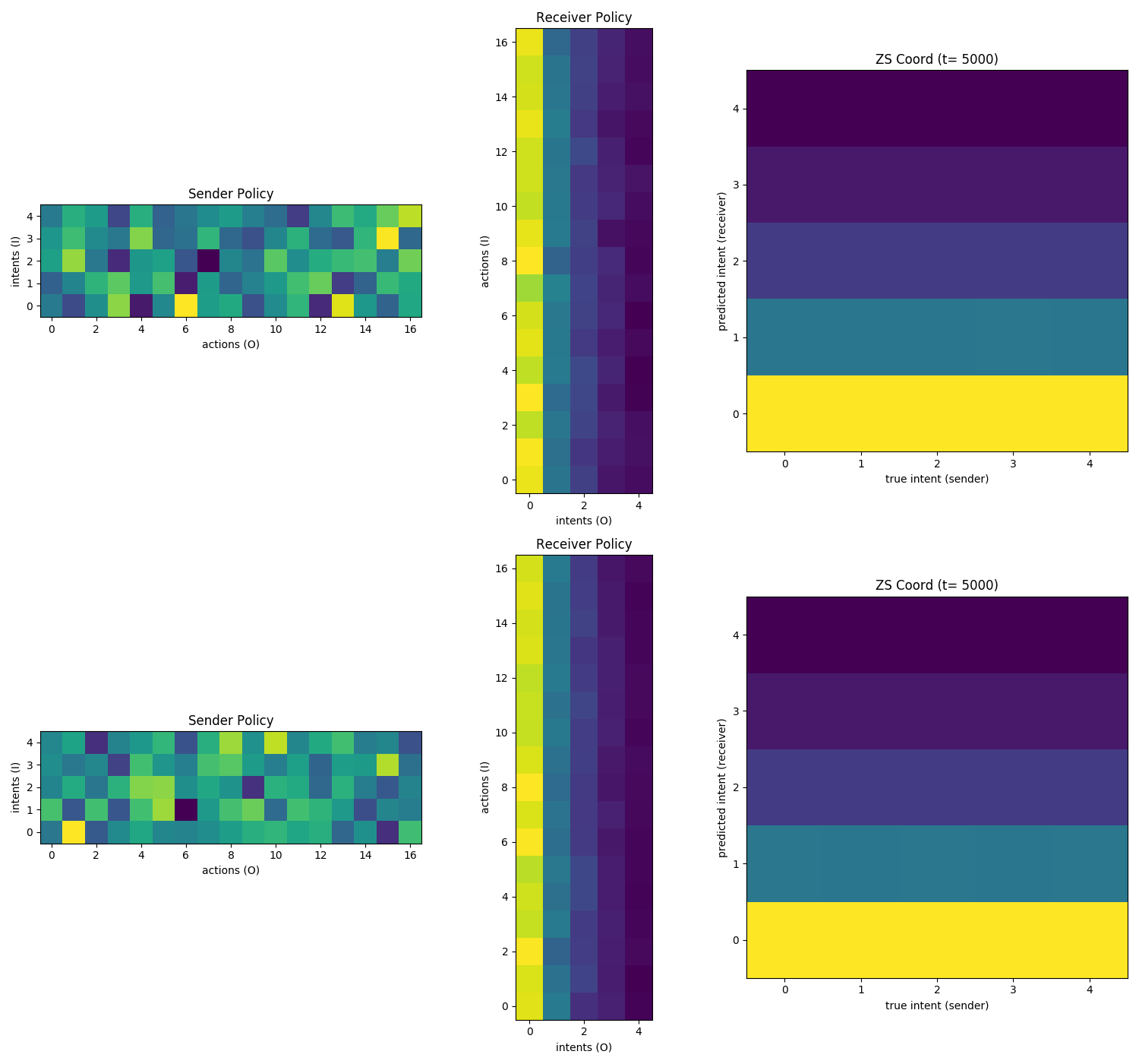
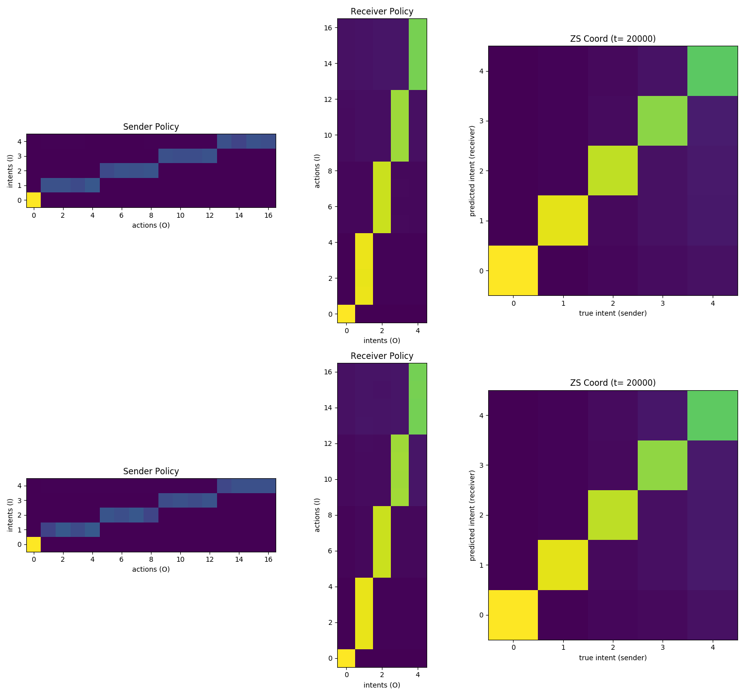
(a) Zipf only (QED): Novel Pairings Tested [XP] (b) Zipf + Engy (QED): Novel Pairings Tested [XP]

Figure 1: Example Policies Learned from Ablation Experiment. Compares Protocols Learned without (left) and with (right) Energy Costs. Energy Degeneracy Task. Two independently trained agent pairs (top, bottom) per condition. Left column shows sender policy mapping given intents to communication actions (messages). Middle column shows receiver policy mapping sender actions to predicted intents. Right column shows SP Performance ($p(predictedIntent\;|\;trueIntent)$) at the end of Protocol Training. All pairs of agents train with a Zipfian Distribution over Intents, for strictly ordering intents by rank, but they differ in whether they employ a cheap talk (left) or costly (right) channel, coupled with that distribution. Illustrates that using the QED algorithm, both conditions converge on policies that will perform consistently with training partners (SP) and novel partners (XP), but only the condition with a nonuniform distribution over intents + the costly communication channel (1(b)) produces policies that are successful in their communication. Intuitively, without a costly channel for mapping intents to specific actions or equivalence classes of actions, the sender policy learns to map each intent a distribution over all actions, and the best the receiver policy can do is make predictions of intent based upon likelihood of observing each intent.

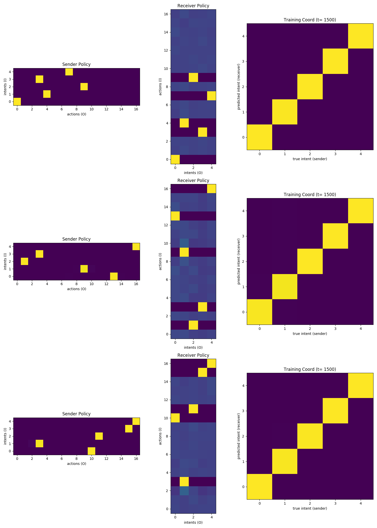
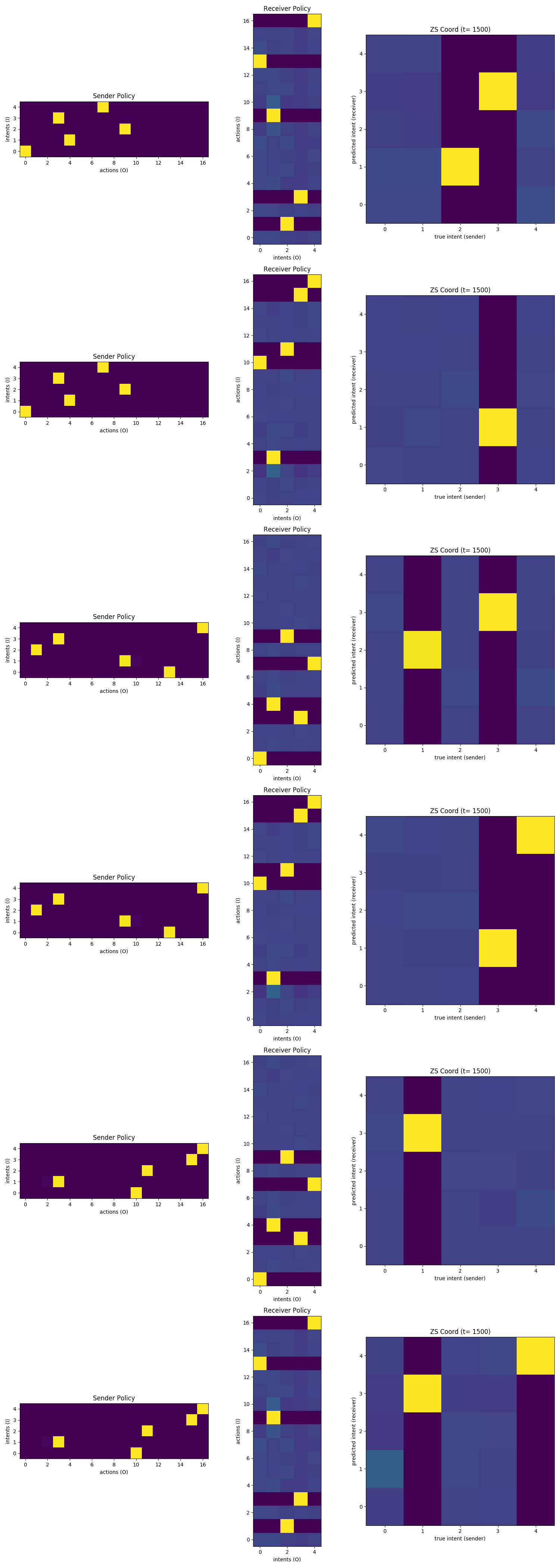
(a) Zipf only (SP): Training Pairs Tested [SP] (b) Zipf only (SP): Novel Pairings Tested [XP]

Figure 2: Protocols Learned and Tested for ZS Coordination using SP training. Energy Degeneracy Task. Zipfian Intent Distribution with Cheap-Talk Channel (only one common knowledge constraint). Protocol Training Coordination (SP) and Zero-Shot Coordination (XP). Illustrates how challenging ZS communication (2(b), right column) is as compared to communication success with training partners (2(a), right column). It is made harder by the fact that policies learned during the initial protocol training phase are very different, across senders (2(a), left column).

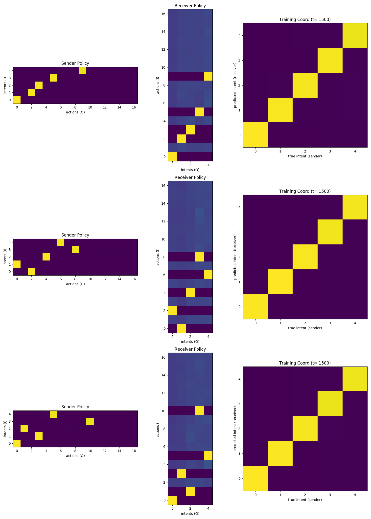
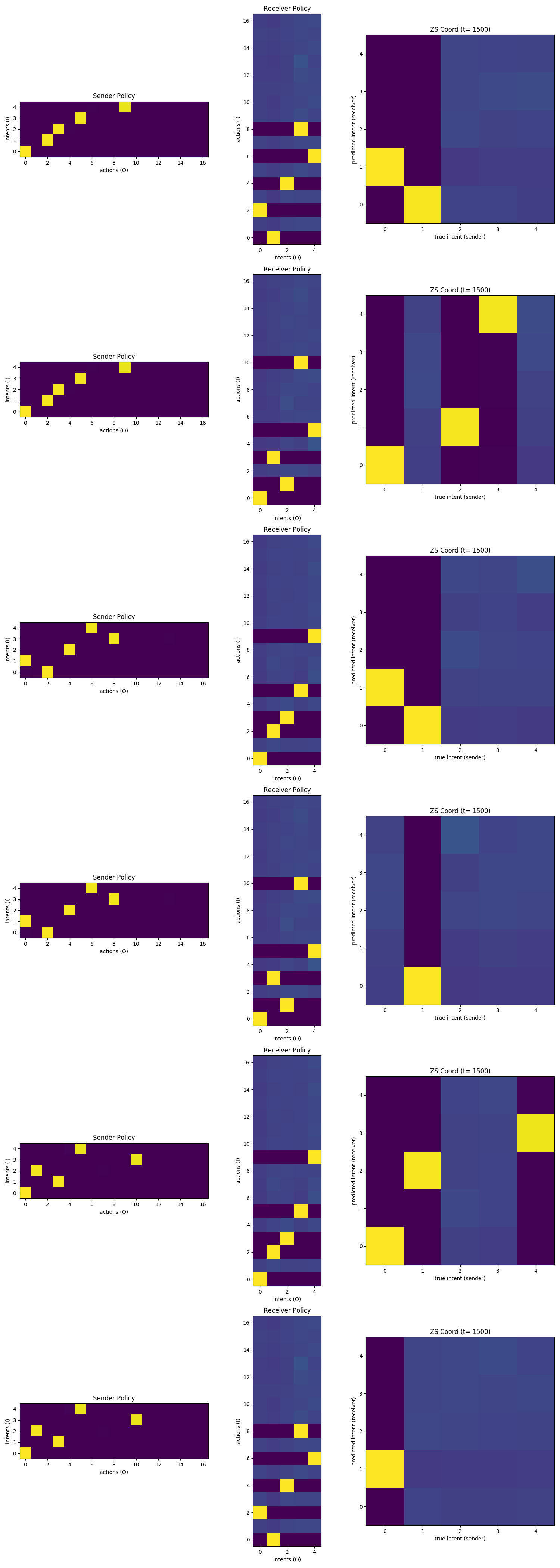
(a) Zipf + Engy (SP): Training Pairs Tested [SP] (b) Zipf + Engy (SP): Novel Pairings Tested [XP]

Figure 3: Protocols Learned and Tested for ZS Coordination using SP training. Energy Degeneracy Task. Zipfian Intent Distribution with Costly Channel (both common knowledge constraints). Protocol Training Coordination (SP) and Zero-Shot Coordination (XP). Illustrates ZS communication (3(b), right column) is substantially more challenging than success with training partners (3(a), right column). Nonetheless, ZS coordination from protocols built upon energy-based latent structure is slightly more successful as compared against ZS coordination in baseline condition with no energy penalty (3(b), right column). The trends observed are similar to that of comparing these two conditions, using QED.