On distributed algorithms for minimum dominating set problem and beyond

Abstract.

In this paper, we study the minimum dominating set (MDS) problem and the minimum total dominating set MTDS) problem which have many applications in real world. We propose a new idea to compute approximate MDS and MTDS. Next, we give an upper bound on the size of MDS of a graph. We also present a distributed randomized algorithm that produces a (total) dominating subset of a given graph whose expected size equals the upper bound. Next, we give fast distributed algorithms for computing approximated solutions for the MDS and MTDS problems using our theoretical results.

The MDS problem arises in diverse areas, for example in social networks, wireless networks, robotics, and etc. Most often, we need to compute MDS in a distributed or parallel model. So we implement our algorithm on massive networks and compare our results with the state of the art algorithms to show the efficiency of our proposed algorithms in practice. We also show how to extend our idea to propose algorithms for solving $k$-dominating set problem and set cover problem. Our algorithms can also handle the case where the network is dynamic or in the case where we have constraints in choosing the elements of MDS.

1. Introduction

This paper deals with fast distributed algorithms to compute dominating set and total dominating set of graphs. Given a graph $G=(V,E)$ with the vertex set $V$ and the edge set $E$, we show the set of adjacent vertices to a vertex $v$, neighbors of $v$, by $N(v)$. A set $S\subseteq V$ is a dominating set of $G$ if each node $v\in V$ is either in $S$ or has a neighbor in $S$. Also, $S\subseteq V$ is a total dominating set of $G$ if each node $v\in V$ has a neighbor in $S$. Let $\gamma(G)$ and $\gamma_{t}(G)$ be the size of a minimum dominating set (MDS) and a minimum total dominating set (MTDS) of a graph $G$ without isolated vertex, respectively. It is easy to prove that

$$\gamma(G)\leq\gamma_{t}(G)\leq 2\gamma(G).$$

An extension of MDS problem is minimum $k$-distance dominating set problem where the goal is to choose a subset $S\subseteq V$ with minimum cardinality such that for every vertex $v\in V\backslash S$, there is a vertex $u\in S$ such that there is a path between them of length at most $k$. The minimum total $k$-distance dominating set is defined similarly.

Also, a subset of vertices such that each edge of the graph is incident to at least one vertex of the subset is a vertex cover. Minimum vertex cover (MVC) is a vertex cover having the smallest possible number of vertices for a given graph. The size of MVC is shown by $\beta(G)$.

An interesting problem is to compute the minimum dominating set and the minimum vertex cover in distributed model. In a distributed model the network is abstracted as a simple $n$-node undirected graph $G=(V,E)$. There is one processor on each graph node $v\in V$, with a unique $\Theta(logn)$-bit identifier $ID(v)$, who initially knows only its neighbors in $G$. Communication happens in synchronous rounds. Per round, each node can send one, possibly different, $O(\log n)$-bit message to each of its neighbors. At the end, each node should know its own part of the output. For instance, when computing the dominating set, each node knows whether it is in the dominating set or has a neighbor in the dominating set (Ghaffari and Kuhn, 2018).

Computing minimum dominating set has many real world applications. Nowadays online social networks are growing exponentially and they have important effect on our daily life. To influence the network participants a key feature in a social network is the ability to communicate quickly within the network. For example, in an emergency situation, we may need to be able to reach to all network nodes, but only a small number of individuals in the network can be contacted directly due to the time or other constraints. However, if all nodes from the network are connected to at least one such individual who can be contacted directly (or is one of those individuals) then the emergency message can be quickly sent to all network participants. In this scenario the goal is to choose the minimum number of such nodes. A challenge is that each node knows its rule instantly.

Also in wireless networks consider the scenario where in order to maximize survivability, the battery power can be conserved by having the minimum possible active sensors, especially for sensors with wide overlapping fields of view. So, we need to find a minimum subset of sensors that need to remain active in order to provide a desirable level of coverage. This scenario is presented in (Sultanik et al., 2010). As another scenario, consider a group of mobile robots each with a wireless access point. The goal of the robots is to maximally cover an area with the wireless network. As the robots are traveling between waypoints, though, it is highly likely that there will be a large amount of overlap in the coverage. Therefore, in order to save power, the robots might want to choose a maximum subset of robots that can lower their transmit power while still retaining coverage(Sultanik et al., 2010). Now suppose that the robots are chosen but suddenly some of them need to be repaired, so the solution should be changed accordingly. The challenge in each of these scenarios is for the agents to collectively find the solution without relying on centralization of computation. Centralization is infeasible either due to lack of resources (i.e., no single agent has powerful enough hardware to solve the global problem) or due to lack of time (i.e., centralizing the problem will take at least a linear number of messaging rounds). Another challenge is that how to solve the problem when some of the inputs are changed or extra constraints are added, for example suppose that some areas should be covered by a specific set of robots or nodes in the network.

The Art Gallery Problem (AGP), a well known problem in computational geometry community, is another problem that is related to MDS problem. There are practical problems that turn out to be related to AGP. Some of these are straightforward, such as guarding a shop with security cameras, or illuminating an environment with few lights. Also the AGP arises in multiagent systems. For example, many robotics, sensor network, wireless networking, and surveillance problems can be mapped to variants of the art gallery problem (Sultanik et al., 2010). The nature of these problems leads us to apply multiagent paradigm, each guard is considered as an agent. So, a new research area is considering the AGP in multiagent paradigm and in distributed model. The AGP is equivalent to the Coverage Problem in the context of wireless sensor networks, wireless ad-hoc networks, and wireless sensor ad-hoc networks (Meguerdichian et al., 2001).

There are also many other problems in networking that can be modeled as the minimum dominating set problem. For example, in (Wang et al., 2013), the problem of node placement for ensuring complete coverage in a long belt with minimum number of nodes scenario is studied. Each node is assumed to be able to cover a disk area centered at itself with a fixed radius. In (Chakrabarty et al., 2002) grid coverage for surveillance and target location in distributed sensor networks is studied.

In social networks the minimum $k$-distance dominating set can be considered as social recommenders. The close nodes influence each other and they have the same preferences in a network. Suppose that we want to give recommendation on a special product (e.g. which movie to watch) to each node of network but we can’t reach all of them because of the time constraint and advertising cost. We may choose minimum number of nodes such that they dominate all other nodes within distance $k$ from them. We give a recommendation to each of the selected nodes and then they spread it in the network. This is equal to solving $k$-dominating set problem. For more on social recommendation see (Gulati and Eirinaki, 2019).

1.1. Recent results and related works

Sequential model

Finding a minimum dominating set is NP-complete (Karp, 1972), even for planar graphs of maximum degree $3$ (Garey and Johnson, 1979), and cannot be approximated for general graphs with a constant ratio under the assumption $P\neq NP$ (Raz and Safra, 1997). An $O(logn)$-approximation factor can be found by using a simple greedy algorithm. Moreover, negative results have been proved for the approximation of MDS even when limited to the power law graphs (Gast et al., 2015). A number of works have been done on exact algorithms for MDS, which mainly focus on improving the upper bound of running time. State of the art exact algorithms for MDS are based on the branch and reduce paradigm and can achieve a run time of $O({1.4969}^{n})$ (van Rooij and Bodlaender, 2011). Fixed parameterized algorithms have allowed to obtain better complexity results (Karthik C. S. et al., 2018). The main focus of such algorithms is on theoretical aspects.

In practice, these theoretical algorithms are not applicable specially in massive networks because of time and space constraints. So we need to use heuristic algorithms to obtain solutions. See (Sanchis, 2002) for a comparison among several greedy heuristics for MDS.

In sequential model heuristic search methods such as genetic algorithm (Hedar and Ismail, 2010) and ant colony optimization (Potluri and Singh, 2011, 2013) have been developed to solve MDS. Also Hyper metaheuristic algorithms combine different heuristic search algorithms and preprocessing techniques to obtain better performance (Potluri and Singh, 2013; Chaurasia and Singh, 2015; Bouamama and Blum, 2016; Lin et al., 2016; Abu-Khzam et al., 2017). These algorithms were tested on standard benchmarks with up to thousand vertices. The configuration checking (CC) strategy (Cai et al., 2011) has been applied to MDS and led to two local search algorithms. Wang et al. proposed the CC2FS algorithm for both unweighted and weighted MDS (Wang et al., 2017), and obtained better solutions than ACO-PP-LS (Potluri and Singh, 2013) on standard benchmarks. Afterwards, another CC-based local search named FastMWDS was proposed, which significantly improved CC2FS on weighted massive graphs (Wang et al., 2018). Chalupa proposed an order-based randomized local search named RLSo (Chalupa, 2018), and achieved better results than ACO-LS and ACO-PP-LS (Potluri and Singh, 2011, 2013) on standard benchmarks of unit disk graphs as well as some massive graphs. Fan et. al. designed a local search algorithm named ScBppw (Fan et al., 2019), based on two ideas including score checking and probabilistic random walk. Recently an efficient local search algorithm for MDS is proposed in (Cai et al., 2020). The algorithm named FastDS is evaluated on some standard benchmarks. FastDS obtains the best performance for almost all benchmarks, and obtains better solutions than previous algorithms on massive graphs in their experiments. A recent study for the $k$-dominating set problem can be found in (Nguyen et al., 2020). They proposed a heuristic algorithm that can handle real-world instances with up to $17$ million vertices and $33$ million edges. They stated that this is the first time such large graphs are solved for the minimum $k$-dominating set problem. They compared their proposed algorithm with the other best known algorithms for this problem.

Distributed model

The centralized algorithms for the MDS and the MTDS problems have been studied well in the literature. However, there is little known about distributed algorithms for these problems. Most of the distributed algorithms proposed to solve the dominating set problem lack giving bounds on both runtime and solution quality. Most of the time the emphasis in the wireless networking community and social networks is on algorithms with a constant number of communication rounds. For example, Ruan et.al. in (Ruan et al., 2004) proposed a one-step greedy approximation algorithm for the minimum connected dominating set problem (MCDS), with an approximation factor that is a function of $\Delta(G)$, where $\Delta(G)$ is the maximum degree of the graph $G$. Kuhn and Wattenhofer (Kuhn and Wattenhofer, 2005) proposed a more general result, their approximation factor is variable and a function of the number of communication rounds. However, this algorithm also depends on $\Delta$. Huang et.al. in (Huang et al., 2006), by increasing the length of messages in each communication round, gave a $12$-approximation algorithm for MCDS problem. For more theoretical results on distributed algorithms for MDS problem see (Amiri et al., 2019).

In (Hilke et al., 2014), it has been shown that for any $\epsilon>0$ there is no deterministic local algorithm that finds a $(7-\epsilon)$- approximation of a minimum dominating set for planar graphs. However, there exist an algorithm with approximation factor of $52$ for computing a MDS in planar graphs (Czygrinow et al., 2008; Lenzen et al., 2013) in local model and an algorithm with approximation factor of $636$ for anonymous networks (Czygrinow et al., 2008; Wawrzyniak, 2013). In (Alipour and Jafari, 2020), they improved the approximation factor in anonymous networks to $18$ in planar graphs without $4$-cycles. For more information on local algorithms see (Suomela, 2013). Then in (Alipour et al., 2020) it has been proved that the approximation factor of (Alipour and Jafari, 2020) for triangle-free planar graphs is 32 and 16 for MDS and MTDS. They have also presented a modified version of the algorithm presented in (Alipour and Jafari, 2020) and implemented their algorithm on real data sets.

Sultanik et al. (Sultanik et al., 2010) introduced a distributed algorithm for the art gallery and dominating set problem that is guaranteed to run in a number communication rounds on the order of the diameter of the visibility graph. They show through empirical analysis that the algorithm will produce solutions within a constant factor of optimal with high probability. The version of AGP that they studied is equivalent to computing MDS of the visibility graph of polygons.

1.2. Our results

In this paper, first we present our theoretical results about computing MDS and MTDS of graphs. We give upper bounds for MDS and MTDS and fast distributed randomized algorithms to achieve these bounds. This upper bound is similar to Caro-Wei bound for maximum independent set of graphs (see (Caro, 1979) and (Wei, 1981)). Next we propose our algorithms for computing the minimum dominating set of graphs using our theoretical results.

In the distributed model the first algorithm runs in constant number of rounds and the communication rounds of the second one depends on the distributed algorithms that are used to find a minimum vertex cover. For example in (Polishchuk and Suomela, 2009) a $3$-approximation for $\beta(G)$ is given that runs in $2\Delta+1$ rounds. In (Åstrand et al., 2009) a $2$-approximation algorithm for $\beta(G)$ is given that runs in $(\Delta+1)^{2}$ rounds.

Our algorithms can be run in dynamic model where the nodes are added or deleted constantly as well. We can handle the case where each node should be dominated by a special set of nodes. Also we show how to to extend the algorithms to solve $k$-distance dominating set problem, and set cover problem.

2. Theoretical Results

In this section, we present our main idea for computing minimum dominating set (MDS) and minimum total dominating set (MTDS) of a given graph $G=(V,E)$. Then we present an upper bound for MDS and MTDS and we give a distributed randomized algorithm for computing this upper bound.

2.1. Main idea

First we present our idea for computing MTDS. Here, we assume all considered graphs have no isolated vertex. For a given graph $G$, we construct a graph $G^{\prime}$ with the same set of vertices as in $G$. For each vertex $v$, we choose two of its neighbors arbitrarily and add an edge between them in $G^{\prime}$, if $v$ is of degree one, we add a loop edge on its neighbor (See Fig 1(a) and 1(b)). We call this edge the corresponding edge of $v$ in $G^{\prime}$ and denote it by $e_{v}$. Note that if the graph $G$ has a cycle of length $4$, with vertices $a,b,c,d$ then the edge $bd$ can be the corresponding edge of both $a$ and $c$ in $G^{\prime}$. So, $|E(G^{\prime})|\leq n$ ($|E(G^{\prime})|$ denotes the size of set $E(G^{\prime})$ and $n$ is the size of the set $V(G)$). Obviously the construction of $G^{\prime}$ can be done in one round in the distributed model. Let $\alpha(G)$ and $\beta(G)$ be the size of maximum independent set and the size of minimum vertex cover of $G$, respectively.

Lemma 2.1.

$\gamma_{t}(G)\leq n-\alpha(G^{\prime})=\beta(G^{\prime}).$

Proof.

Suppose that $D$ is a maximum independent set of $G^{\prime}$, so $|D|=\alpha(G^{\prime})$. Now we show that $V\backslash D$ is a total dominating set for $G$. For each vertex $v$, we choose two of its neighbors, for example $u$ and $w$, and add an edge between them in $G^{\prime}$. Since there is an edge between $u$ and $w$, so at most one of them can be in $D$ which means at least one of them is in $V\backslash D$. The same argument applies when an edge is a loop. Thus for each vertex $v$ at least one of its neighbors in $G$ is in $V\backslash D$, so $V\backslash D$ is a total dominating set for $G$. The size of $|V\backslash D|$ equals $n-\alpha(G^{\prime})$ and we have $\gamma_{t}(G)\leq n-\alpha(G^{\prime})=\beta(G^{\prime})$. ∎

Note that $G^{\prime}$ is not unique, so there is a set $A$ of graphs $G^{\prime}_{i}$’s such that they can be constructed as we explained earlier. Now we present our main theorem.

Theorem 2.2.

Let $G^{\prime}_{min}\in A$ be such that

$$n-\alpha(G^{\prime}_{min})=min_{G^{\prime}_{i}\in A}{n-\alpha(G^{\prime}_{i})},$$

then

$$\gamma_{t}(G)=n-\alpha(G^{\prime}_{min})=\beta(G^{\prime}_{min}).$$

Proof.

By Lemma 2.1 we have $\gamma_{t}(G)\leq\beta(G^{\prime}_{min})$. To show that $\beta(G^{\prime}_{min})\leq\gamma_{t}(G)$, it is enough to construct a graph $G^{\prime}\in A$ such that $\beta(G^{\prime})=\gamma_{t}(G)$. Let $S$ be a total dominating set of vertices of cardinality $\gamma_{t}(G)$. For each vertex $v\in V$, there is at least one vertex $u\in S$ such that $u$ and $v$ are adjacent. If $d(v)=1$ then, we put a loop on its neighbor, $u$, otherwise $v$ has at least another neighbor, for example $w$. We put an edge between $u$ and $w$. Now we have our graph $G^{\prime}\in A$. Since every edge of $G^{\prime}$ has at least one of its endpoints in $S$, hence $S$ is a vertex cover for $G^{\prime}$. On the other hand, any vertex cover for $G^{\prime}$ is a total dominating set for $G$, since for any vertex $v$ of $G$ there is an edge of $G^{\prime}$ whose endpoints are adjacent to $v$, hence it is dominated by a vertex cover of $G^{\prime}$. Therefore $S$ is a minimum dominating set for $G^{\prime}$ and we have $\beta(G^{\prime})=\gamma_{t}(G)$ (See Fig 1(c)).

∎

Figure 1. Graph $G$ with $\gamma_{t}(G)=3$ and the constructed graphs from $G$.

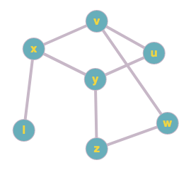
(a) Graph $G$ with a MDTS of size 3. For example $\{v,x,y\}$ is a MTDS for $G$.

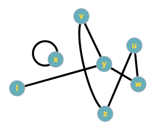
(b) Graph $G^{\prime}$ which is constructed from $G$. Here, $e_{v}=uw$, $e_{u}=vy$, $e_{y}=uz$, $e_{w}=vz$, $e_{z}=wy$, $e_{x}=vy$ and $e_{i}=xx$, where by $xx$ we mean a loop on $x$ and $\beta(G^{\prime})=4$. For example $\{x,y,z,w\}$ is a minimum vertex cover for $G^{\prime}$ and a dominating set for $G$.

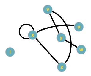
(c) Here the Graph $G^{\prime}_{min}$ is also constructed from $G$. Here, $e_{v}=ux$, $e_{u}=vy$, $e_{x}=vy$, $e_{y}=xz$, $e_{w}=vz$, $e_{z}=wy$ and $e_{i}=xx$ and $\beta(G^{\prime}_{min})=3$. For example $\{x,v,y\}$ is a minimum vertex cover for $G^{\prime}_{min}$ and a minimum total dominating set for $G$.

Now we give a similar argument for computing MDS. We construct a graph $G^{\prime\prime}$ from $G$ as follows. The vertex set of $G^{\prime\prime}$ is the same as $G$. For each vertex $v\in V$ we choose two vertices from $N(v)\bigcup v$ and add an edge between those two selected vertices. This way we have a graph $G^{\prime\prime}$. For MDS we do not have the assumption that there is no isolated vertices. So if $v$ is isolated we simply put a loop on $v$.

Lemma 2.3.

$\gamma(G)\leq n-\alpha(G^{\prime\prime})=\beta(G^{\prime\prime}).$

Since $G^{\prime\prime}$ is not unique, so there is a set $A$ of graphs $G^{\prime\prime}_{i}$’s such that they can be constructed as we explained earlier. We have the following theorem.

Theorem 2.4.

Let $G^{\prime\prime}_{min}\in A$ be such that

$$n-\alpha(G^{\prime\prime}_{min})=min_{G^{\prime\prime}_{i}\in A}{n-\alpha(G^{\prime\prime}_{i})},$$

then

$$\gamma(G)=n-\alpha(G^{\prime\prime}_{min})=\beta(G^{\prime\prime}_{min}).$$

We omit the proofs because they are similar to the proofs of Lemma 2.1 and Theorem 2.2. As we said earlier $G^{\prime}$ and $G^{\prime\prime}$ are not unique. So, our aim is to give algorithms for constructing $G^{\prime}$ and $G^{\prime\prime}$ such that $\beta(G^{\prime})$ and $\beta(G^{\prime\prime})$ be a good approximation of $\beta(G^{\prime}_{min})$ and $\beta(G^{\prime\prime}_{min})$.

As a result of Lemma 2.1 and Lemma 2.3 in the following subsection we present an upper bound for MDS and MTDS.

2.2. An upper bound for MDS and MTDS and a distributed algorithm for computing that bound

To compute an upper bound for MTDS of a graph $G$, we construct a graph $G^{\prime}$ as before. By Lemma 2.1, $\gamma_{t}(G)\leq n-\alpha(G^{\prime})$. Caro (Caro, 1979) and Wei (Wei, 1981) showed that in a given graph $G$, $\sum^{n}_{i=1}\frac{1}{1+d_{i}}\leq\alpha(G)$, where $d_{i}$ is the degree of vertex $i$. So, we have the following theorem.

Theorem 2.5.

By Lemma 2.1 and Lemma 2.3 if we construct the graphs $G^{\prime}$ and $G^{\prime\prime}$ arbitrarily then,

$$\gamma_{t}(G)\leq n-\alpha(G^{\prime})\leq n-\sum^{n}_{i=1}\frac{1}{1+d_{i}^{\prime}}.$$

Where $d_{i}^{\prime}$ is the degree of $v_{i}$ in $G^{\prime}$. And

$$\gamma(G)\leq n-\alpha(G^{\prime\prime})\leq n-\sum^{n}_{i=1}\frac{1}{1+d_{i}^{{}^{\prime\prime}}}.$$

Where $d_{i}^{{}^{\prime\prime}}$ is the degree of $v_{i}$ in $G^{\prime\prime}$.

These bounds for MTDS and MDS is similar to Caro and Wei bound for independent set of graphs.

A randomized distributed algorithm for computing the given upper bound for MTDS and MDS

An independent set of expected size $\sum^{n}_{i=1}\frac{1}{1+d_{i}}$ for a graph $G$ can be found by a simple linear time randomized algorithm that follows from an analysis of the Caro-Wei bound by Alon and Spencer in (Alon and Spencer, 2004). This algorithm works as follows. Every node $v$ chooses a random real value between $0$ and $1$ and adds itself to the independent set $I$ if none of its neighbors have chosen a larger real value than $v$. Then, the probability that a node $v$ is added to the independent set is $\frac{1}{1+d_{i}}$, hence by linearity of expectation, $E(I)=\sum^{n}_{i=1}\frac{1}{1+d_{i}}$.

So, our distributed algorithm to compute an upper bound for MTDS is as follows. We construct a graph $G^{\prime}$ arbitrary as explained and then compute an independent set of expected size of $\sum^{n}_{i=1}\frac{1}{1+d^{\prime}_{i}}$. We choose those vertices that are not in the independent set of $G^{\prime}$. Which means that we compute a total dominating set of expected size of $n-\sum^{n}_{i=1}\frac{1}{1+d^{\prime}_{i}}$ in constant number of rounds. The same argument applies for the MDS. We construct a graph $G^{\prime\prime}$ and then we compute a vertex cover of expected size of $n-\sum^{n}_{i=1}\frac{1}{1+d^{{}^{\prime\prime}}_{i}}$.

3. Algorithms

In this section we present two distributed algorithms for computing a dominating set for a given graph.

3.1. First Algorithm

The first algorithm is the same as algorithm presented in (Alipour et al., 2020) with a small modification. In (Alipour et al., 2020), they compute a total dominating set and since a total dominating set is also a dominating set in graphs with no isolated vertex, they consider this total dominating set as a dominating set. But in our modified version we compute a dominating set. As we said earlier the size of MTDS can be twice of the size of MDS so in practice we expect that this algorithm performs better than the algorithm in (Alipour et al., 2020).

1:  In the first round, each node $v_{i}$ chooses a random number $0<r_{i}<1$ and computes its weight $w_{i}=d_{i}+r_{i}$ and sends $w_{i}$ to its adjacent neighbors.

2:  In the second round, each node $v$ marks a vertex $v_{i}\in N(v)\bigcup v$, whose weight $w_{i}$ is maximum among all the other neighbors of $v$.

3:  for $m$ rounds do

4:     Let $x_{i}$ be the number of times that a vertex is marked by its neighbor vertices, let $w_{i}=x_{i}+r_{i}$

5:     Unmark the marked vertices.

6:     Each vertex $v$ marks the vertex with $v_{i}\in N(v)\bigcup v$ maximum $w_{i}$.

7:  end for

8:  The marked vertices are considered as the vertices in our dominating set for $G$.

Algorithm 1 First distributed algorithm for computing a dominating set in a graph with given integer $m\geq 0$.

Obviously the set of marked vertices is a dominating set since each vertex marks itself or one of its neighbors. In the first round, $r_{i}$’s are generated and added to $d_{i}$’s. And in the next round each vertex mark a vertex with maximum $w_{i}$. In the next $m$ rounds each vertex marks a vertex based on $x_{i}$’s. So, in a distributed network for a constant number $m$, this algorithm runs in constant number of rounds. Note that this algorithm is the same as (Alipour et al., 2020), except that in line 2 and line 6 of Algorithm 1 each vertex marks a vertex in $v\bigcup N(v)$ but in (Alipour et al., 2020), each vertex $v$ marks a vertex in $N(v)$. That is why their algorithm gives a total dominating set but Our algorithm gives a dominating set.

3.2. Second Algorithm

In the second algorithm our aim is to improve the results of Algorithm 1 by using Theorem 2.4. First we run Algorithm 1. In this algorithm at the last step for each $v_{i}$ we know the value of $x_{i}$, i.e. the number of times that vertex $v_{i}$ is selected by its neighbors or itself. We construct a graph $G^{\prime\prime}_{1}$ from $G$ as follows. The vertex set of $G^{\prime\prime}_{1}$ is the same as $G$. For each vertex $v_{i}$ in $G$ we choose two vertices $u_{i},y_{i}\in N(v_{i})\bigcup v_{i}$ with maximum value of $x_{j}+r_{j}$’s such that $x_{j}>0$. Then we add an edge between $u_{i}$ and $y_{i}$ in $G^{\prime\prime}_{1}$ and if there is only one $x_{j}>0$ we add a loop on $v_{j}$.

Algorithm 2 Second distributed algorithm for computing dominating set in a given graph.

1:  Run Algorithm 1 for $m$ rounds.

2:  Let $G^{\prime\prime}_{1}$ be a graph with the same vertex set as $G$.

3:  For each vertex $v_{i}$ choose two vertices $u_{i},y_{i}\in N(v_{i})\bigcup v_{i}$ with maximum values of $x_{j}+r_{j}$’s such that $x_{j}>0$. Add an edge between $u_{i}$ and $y_{i}$ in $G^{\prime\prime}_{1}$ and if there is only one $x_{j}>0$ we add a loop on $v_{j}$.

4:  Compute a vertex cover for $G^{\prime\prime}_{1}$ which is a dominating set for $G$.

By Lemma 2.1, if we compute a vertex cover for $G^{\prime\prime}_{1}$ then the vertices in the vertex cover of $G^{\prime\prime}_{1}$ form a dominating set for $G$. Obviously $G^{\prime\prime}_{1}$ can be constructed in constant number of rounds in distributed model. There are well known algorithms for computing the minimum vertex cover of a graph in distributed model which according to our running time and space constraints we can use one of them.

In this section we explained two algorithms for computing a dominating set for graphs. We are not able to compute the approximation factor of these algorithms theoretically in general. Instead we implement the algorithms on real data sets and compare the results with state of the art algorithms.

4. Experiments

Data description

In the following we present a brief description of the benchmarks from (Cai et al., 2020).

T1: This data set consists of $520$ instances where each instance has two different weight functions. As in (Cai et al., 2020) we select these original graphs where the weight of each vertex is set to $1$. There are $52$ families, each of which contains $10$ instances with the same size. The instances have 50 to 1000 nodes with different number of randomly created edges but always making the graph connected (for more details see (ROMANIA, 2010)).

BHOSLIB: This benchmark are generated based on the RB model near the phase transition. It is known as a popular benchmark for graph theoretic problems. The order of average number of vertices in this benchmark is about $750$ and average number of edges is about $10^{5}$ (for more details see (Rossi and Ahmed, 2015)).

SNAP: This benchmark is from Stanford Large Network Dataset Collection. It is a collection of real world graphs from $10^{4}$ vertices to $10^{7}$ vertices (for more details see (Leskovec and Krevl, 2014)).

DIMACS10: This benchmark is from the 10th DIMACS implementation challenge, which aims to provide large challenging instances for graph theoretic problems (for more details see (Rossi and Ahmed, 2015)).

Network Repository: The Network Data Repository includes massive graphs from various areas. Many of the graphs have $100$ thousands or millions of vertices. This benchmark has been widely used for graph theoretic problems including vertex cover, clique, coloring, and dominating set problems. As in (Cai et al., 2020) for SNAP benchmarks we consider the graphs with at list $30000$ vertices and for Repository benchmark we choose the graphs with at least $10^{5}$ vertices (for more details see (Rossi and Ahmed, 2015)).

Experimental results and implementation

The most related work to ours is in (Alipour et al., 2020), where their local distributed algorithm computes a total dominating set for graphs and since a total dominating set is also a dominating set so they implemented and ran their algorithm on some real data sets and compared their results with a recent centralized algorithm for minimum dominating set problem in (Cai et al., 2020).

In Table 1, Table 2, Table 3 and Table 4 we present our results and compare the results with (Alipour et al., 2020). The first column is the output of Algorithm 2 with two modifications. The first modification is that instead of line 1, we run algorithm presented in (Alipour et al., 2020) for $m=5$ iterations. And the second modification is that in line 4, instead of choosing $u_{i}$ and $y_{i}$ from $N(v_{i})\bigcup v_{i}$, we choose them from $N(v_{i})$. In this case the achieved dominating set is also a total dominating set. We call this modified 1 of Algorithm 2 (Mod1). In the second column we run Algorithm 2 with a modification in line $1$ as follows. Instead of algorithm 1 we run the algorithm in (Alipour et al., 2020) for $m=5$ iterations. We call this Modified 2 of Algorithm 2 (Mod2). In the third and forth columns the results of Algorithm 2 and Algorithm 1 for $m=5$ are presented. In sixth column the results of implementation of the algorithm in (Alipour et al., 2020) is presented. And in the last column we present the results of algorithm presented in (Cai et al., 2020). The empty cells were not computed in (Cai et al., 2020).

Table 1. Experimental results for T1 benchmark.

Instance	Mod1	Mod2	Alg 2	Alg 1	(Alipour et al., 2020)	(Cai et al., 2020)
V100E100	42	42	42	50	50	34
V100E1000	10	10	10	12	12	8
V100E2000	6	6	6	6	6	5
V100E250	28	28	28	29	29	20
V100E500	16	16	16	18	18	13
V100E750	12	12	12	12	12	9
V150E1000	21	21	21	22	22	15
V150E150	63	63	63	73	73	50
V150E2000	12	12	12	13	13	9
V150E250	46	46	46	51	51	39
V150E3000	11	11	11	11	11	7
V150E500	31	31	31	36	36	25
V150E750	25	25	25	26	26	18
V200E1000	32	32	32	34	34	24
V200E2000	22	22	22	22	22	15
V200E250	80	80	80	87	87	61
V200E3000	13	13	13	14	14	11
V200E500	54	54	54	55	55	37
V200E750	41	41	41	44	44	30
V250E1000	49	49	49	52	52	36
V250E2000	30	30	30	31	31	22
V250E250	106	106	106	122	122	83
V250E3000	24	24	24	25	25	16
V250E500	77	77	77	87	87	58
V250E5000	16	16	16	17	17	11
V250E750	62	62	62	64	64	44
V300E1000	62	62	62	70	70	49
V300E2000	40	40	40	43	43	29
V300E300	128	128	128	141	141	100
V300E3000	30	30	30	31	31	22
V300E500	107	107	107	115	115	78
V300E5000	22	22	22	23	23	15
V300E750	86	86	86	89	89	60
V500E1000	150	150	150	165	165	115
V500E10000	35	35	35	35	35	22
V500E2000	104	104	104	114	114	71
V500E500	214	214	214	241	241	167
V500E5000	58	58	58	59	59	37
V800E1000	326	326	326	355	355	267
V800E10000	80	80	80	85	85	50
V800E2000	222	222	222	239	239	158
V800E5000	121	121	121	129	129	83
V1000E1000	417	417	417	476	476	334
V1000E10000	110	110	110	118	118	74
V1000E15000	80	80	80	85	85	55
V1000E20000	73	73	73	76	76	45
V1000E5000	184	184	184	194	194	121

Table 2. Experimental results for BHOSLIB benchmark.

Instance	Mod1	Mod2	Alg 2	Alg 1	(Alipour et al., 2020)	(Cai et al., 2020)
frb40-19-1	2	2	2	3	3	14
frb40-19-2	3	3	4	4	3	14
frb40-19-3	4	4	4	4	4	14
frb40-19-4	3	3	3	4	4	14
frb40-19-5	3	3	3	3	3	14
frb45-21-1	3	3	3	4	4	16
frb45-21-2	4	5	3	4	5	16
frb45-21-3	3	3	3	3	3	16
frb45-21-4	4	4	4	4	4	16
frb45-21-5	3	3	3	3	3	16
frb50-23-1	3	3	3	4	4	18
frb50-23-2	4	4	4	4	4	18
frb50-23-3	3	3	3	3	4	18

In BHOSLIB the achieved results are surprisingly better than (Cai et al., 2020). In dense graphs or the graphs with large maximum degree, close to n (number of vertices), the adjacent vertices to the maximum degree choose it, so the number of marked vertices is small and close to the exact solution. For example in instance frb40-19-1 of BHSLIB benchmark, the number of vertices is about 760, the maximum degree is 703, the minimum degree is 581 and the average degree is 650.

Table 3. Experimental results for Network snap and DIMACS10 benchmark.

Instance	Mod1	Mod2	Alg 2	Alg 1	(Alipour et al., 2020)	(Cai et al., 2020)
Amazon0302(V262K E1.2M)	46602	43965	42095	45742	49903	35593
Amazon0312(V400K E3.2M)	56034	53640	52707	57068	59723	45490
Amazon0505(V410K E3.3M)	58088	55717	54687	59241	61905	47310
Amazon0601(V403K E3.3M)	52132	50298	49464	53432	55644	42289
email-EuAll(V265K E420K)	33852	31468	18185	18219	33864	18181
p2p-Gnutella24(V26K E65K)	5557	5515	5476	5655	5718	5418
p2p-Gnutella25(V22K E54K)	4645	4610	4594	4756	4807	4519
p2p-Gnutella30(V36K E88K)	7336	7281	7263	7449	7524	7169
p2p-Gnutella31(V62K E147K)	12793	12703	12676	12980	13115	12582
soc-sign-Slashdot081106(V77K E516K)	14975	14420	14390	14865	15209	14312
soc-sign-Slashdot090216(V81K E545K)	16118	15484	15446	16010	16418	15305
soc-sign-Slashdot090221(V82K E549K)	16154	15517	15490	16021	16436	-
soc-Epinions1(V75K E508K)	16557	15840	15789	16255	16760	15734
web-BerkStan(V685K E7.6M)	37711	35039	31784	33980	39938	28432
web-Stanford(V281K E2.3M)	18350	16887	15032	16176	19643	13199
wiki-Talk(V2.3M E5M)	40135	39324	36969	37219	40191	36960
wiki-Vote(V7K E103K)	1153	1143	1121	1150	1177	1116
cit-HepPh(V34K E421K)	3812	3701	3624	3905	4074	3078
cit-HepTh(V27K E352K)	3764	3553	3386	3684	4025	2936
rgg-n-2-17-s0	21605	20495	19282	21430	23523	43412
rgg-n-2-19-s0	80038	76081	71875	79557	86742	844423
rgg-n-2-20-s0	153393	146039	138412	153129	166522	84708
rgg-n-2-21-s0	295851	281372	267307	295447	320642	162266
rgg-n-2-22-s0	571868	545511	518014	572266	619551	312350
rgg-n-2-23-s0	1107851	1057773	1006686	1110615	1199233	605278
coAuthorsCiteseer	37005	34508	34139	36381	38310	22011
co-papers-citeseer	34647	32114	31330	34874	37057	26082
kron-g500-logn16	14120	14118	14117	14171	14174	14100
co-papers-dblp	48638	45467	44805	49821	52187	43978

Table 4. Experimental results for Network repository benchmark.

Instance	Mod1	Mod2	Alg 2	Alg 1	(Alipour et al., 2020)	(Cai et al., 2020)
soc-youtube(V496 E2M)	99669	92020	91192	96212	102355	89732
soc-flickr(V514K E3M)	104571	99237	98832	102194	106337	98062
ca-coauthors-dblp(V540K E15M)	48647	45533	44833	49841	52180	35597
ca-dblp-2012(V317K E1M)	50246	47497	47067	49669	51790	46138
ca-hollywood-2009(V1.1 E56.3)	58060	57072	56972	61096	61626	48740
inf-roadNet-CA(V2M E3M)	834653	785263	718224	790165	911273	586513
inf-roadNet-PA(V1M E2M)	464398	436853	400628	440939	507130	326934
rt-retweet-crawl(V1M E2M)	82927	76039	75825	76916	83368	75740
sc-ldoor(V952k E21M)	77595	75189	70543	73017	79629	62411
sc-pwtk(V218K E6M)	8783	8228	7321	8077	9444	4200
sc-shipsec1(V140K E2M)	13908	13638	13361	14405	14926	7662
sc-shipsec5(V179K E2M)	20512	20179	19940	21689	22184	10300
soc-FourSquare(V639K E3M)	61324	61324	61324	62053	62053	60979
soc-buzznet(V101K E3M)	138	138	138	150	150	127
soc-delicious(V536K E1M)	57795	56192	56067	57131	58491	55722
soc-digg(V771K E6M)	70185	67240	66896	69234	71889	66155
soc-flixster(V3M E8M)	91528	91044	91035	91312	91605	91019
soc-lastfm(V1M E5M)	67445	67270	67258	67466	67621	67226
soc-livejournal(V4M E28M)	855807	826813	822403	868615	891958	793887
soc-orkut(V3M E106M)	141426	141267	141208	151742	151881	110547
soc-pokec(V2M E22M)	234696	231289	230622	245806	248740	207308
soc-youtube-snap(V1M E3M)	231538	215321	214338	222480	234965	213122
socfb-FSU53(V28K E1M)	2388	2379	2369	2575	2589	-
socfb-Indiana69(V30K E1M)	2301	2289	2278	2435	2450	-
socfb-MSU24(V32K E1M)	2837	2806	2797	2996	3020	-
socfb-Michigan23(V30K E1M)	2708	2681	2663	2851	2893	-
socfb-Penn94(V42K E1M)	3836	3809	3802	4096	4116	-
socfb-Texas80(V32K E1M)	2787	2770	2750	2984	3010	-
socfb-Texas84(V36K E2M)	2840	2830	2822	3061	3073	-
web-edu	252	249	249	251	253	-
web-polblogs	115	109	108	113	118	-
web-spam	889	858	854	901	925	-
web-indochina-2004	1513	1496	1491	1504	1517	-
web-webbase-2001	1112	1064	1055	1114	1158	-
web-sk-2005	31166	30014	29046	30128	32306	-
web-uk-2005	1715	1421	1421	1587	1717	1421
web-arabic-2005	19518	18191	17676	18533	20288	-
web-Stanford	18398	16924	15001	16155	19678	-
web-it-2004	34066	33233	33183	34017	34442	32997
web-italycnr-2000	23832	22827	22665	23304	24372	-

The running time of (Alipour et al., 2020) and Algorithm 1 are the same since they have a small difference which does not affect the running time. But as it can be seen the quality of solution in Algorithm 1 is better than (Alipour et al., 2020). Because in (Alipour et al., 2020) they compute a total dominating set but we compute a dominating set. Essentially the size of MTDS can be twice of the size of MDS so this can explain why this happens.

The running time of algorithm 2 depends on the algorithm used for computing MCV of $G^{\prime\prime}$. In our experiment we have used a $2$-approximation factor algorithm for computing MVC. Theoretically the quality of solution in Algorithm 2 is better than Algorithm 1. Because in graph $G^{\prime\prime}$ which is constructed from $G$ based on Theorem 2.4, the edges are added between the vertices which are marked in Algorithm 1, obviously the size of vertex cover of $G^{\prime\prime}$ is less than or equal the number of total vertices marked in Algorithm 1. On the other hand Algorithm 1 is faster than Algorithm 2.

Note that the running time of the modified versions of algorithms (column 1 and column 2) is the same as Algorithm 2. In all of the instances Algorithm 2 performs better than Mod1 and Mod2 except two instances.

The first modified version computes a total dominating set and we can compare the results with (Alipour et al., 2020) which also computes a total dominating set. As it can be expected Mod1 performs better than (Alipour et al., 2020).

Note that (Cai et al., 2020) is a recent sequential algorithm for computing dominating set and they have done many experiments and compared their results with state of the art algorithms. Their algorithm performs better than the other algorithms in most of the times. As we explain earlier, theoretically improving the approximation factor of MDS in distributed model is a challenging problem. If we compare our results with (Cai et al., 2020) we can see that either our algorithms solution quality is better than their algorithm for example in BHOSLIB data set, or our solutions are at most two times of their solutions. This shows that in practice the proposed algorithms have acceptable solutions in distributed model.

Note that we have implemented a centralized version of our proposed algorithms. In centralized version the nodes mark a vertex one by one, but in distributed version this is done by all nodes in one round. So, solution set in both centralized and sequential implementation is the same. However we can modify the algorithms in sequential model to get better solutions which is not our aim in this paper and we have focused on distributed algorithms. The experiments were run in a system with OS: CentOS Linux release 7.7.1908 (Core), CPU: Intel E5-2683 v4 Broadwell $@$ 2.1Ghz and Memory: 100G. The codes are also available in the web.

We have run the algorithms for each instance just once. In the first step we assign a random number $r_{i}$ for each vertex. This can affect the solution in the case where two vertices $v_{i}$ and $v_{j}$ have a common neighbor $v$ and $d_{i}=d_{j}$ and their degree is maximum among $N(v)$. Here , $v$ marks one of them based on $r_{i}$ and $r_{j}$. So, if we run the algorithm several times and choose the minimum solution, better results can be achieved.

5. Remarks, importance and applications of proposed algorithms

Set cover problem

In the set cover problem we are given a set $A=\{a_{1},a_{2},\dots a_{n}\}$ of $n$ elements and $m$ subsets, $A_{1},A_{2},\dots,A_{m}$ of $A$. The goal is to choose the minimum number of subsets that cover all the elements of $A$. In (Alipour et al., 2020) they have explained how to change their algorithm to choose the subsets. Each element $a$ chooses a subset $A_{j}$ with maximum size such that $a_{i}\in A_{j}$. Let $x_{i}$’s be the number of times that $A_{i}$’s are chosen by the elements. Next round each $a_{i}$ chooses a subset $A_{j}$ such that $a_{i}\in A_{j}$ with maximum $x_{i}+r_{i}$. For $m$ rounds the previous step is repeated.

Now we explain how to modify Algorithm 2 to solve set cover problem. First we run the modified version of (Alipour et al., 2020). Next we construct a graph $G^{\prime}$ that its vertices are the subsets $A_{1},A_{2},\dots,A_{m}$. For each $a\in A$ we choose two subsets $A_{i}$ and $A_{j}$ with maximum values of $x_{i}$s such that $a\in A_{i}$ and $a\in A_{j}$ and add an edge between them. Similar to the proof of Lemma 2.1 It can be shown that a vertex cover for $G^{\prime}$ is a set cover for $A$.

$k$-distance dominating set

A $k$-observer $Ob$ of a network $N$ is a set of nodes in $N$ such that each message, that travels at least $k$ hops in $N$, is handled (and so observed) by at least one node in $Ob$. A $k$-observer $Ob$ of a network $N$ is minimum iff the number of nodes in $Ob$ is less than or equal the number of nodes in every $k$-observer of $N$ (See (Chakrabarty et al., 2002)). This problem is equivalent to the $k$-distance dominating set problem. In this problem for each node $v$, the neighbors of $v$, is the set of nodes that their distance from $v$ is less than $k+1$. Then we apply the proposed algorithms as before.

Note that computing a minimum $k$-distance dominating set for a graph $G$ is equivalent to computing a minimum dominating set for $G^{k}$, where $G^{k}$ is a graph with the same vertex set as $G$ and we put an edge between two vertices in $G^{k}$ if the distance between them in $G$ is less that $k+1$. Since our algorithms performs well in dense graphs so if $G$ is a dense graph then as the value of $k$ increases the graph $G^{k}$ will be denser and the quality of solution of our proposed algorithm will be improved.

Other variations and constraints

Suppose that the network is dynamic and nodes and edges are added or deleted constantly for example some nodes are online only in particular period of time. In dynamic model, for example when a vertex $v$ with its adjacent edges are added we only need to change the marked vertices that are chosen by $N(v)$ and $N(N(V))$ in Algorithm 1. In Algorithm 2, only the corresponding edges of $N(v)$ and $N(N(v))$ are modified because the value of $x_{i}$’s for $N(v)$ is changed. This modification is done locally.

In some situations each vertex $v$ should be dominated by a specific set of vertices denoted by $A_{v}\subset N(v)$. In this case, in Algorithm 1, $v_{i}$ marks a vertex $v_{j}\in(N(v)\bigcup v)\bigcap A_{v}$ with maximum $w_{j}$. Similarly in Algorithm 2, for a vertex $v$ we choose two vertices with maximum $w_{i}$’s from $(N(v)\bigcup v)\bigcap A_{v}$. In practice, for example in a sensor network suppose the case where the coverage radius of each sensor is limited for example less than $d$. And each sensor covers limited angular direction.

Remarks

In obtaining the upper bound, we can use other known algorithms for computing the minimum vertex cover and maximum independent set of graphs to achieve better bounds.

We believe that Algorithm 2 is a powerful tool for computing good approximation factor solutions for MDS and MTDS of graphs in distributed model. In Algorithm 2 or in its modified versions we try to use good candidates as our dominating set for constructing $G^{\prime}$ and $G^{\prime\prime}$. So we use the output of Algorithm 1 or the algorithm of (Alipour et al., 2020). As a future work one can use other algorithms or ideas to choose the vertices for adding edges between them in constructing $G^{\prime}$ and $G^{\prime\prime}$.

Also it might be useful to construct the graphs $G^{\prime}$ and $G^{\prime\prime}$ according to the topology of the network and in a more data sensitive way.

The important property of Algorithm 2 is that $G^{\prime}$ and $G^{\prime\prime}$ can be constructed in distributed model. The rest is computing the vertex cover of $G^{\prime}$ and $G^{\prime\prime}$ which are well studied in the distributed model and we can use the known distributed algorithms for computing the minimum vertex cover. Beside the distributed nature of our proposed algorithms, it can easily seen that these algorithms can be applied on big data as well. The proposed algorithms are very fast and easy to implement and they need low storage.

Note that the idea of constructing $G^{\prime}$ and $G^{\prime\prime}$ from $G$ can help us to combine the algorithms to get a better solution. For example suppose that there are two algorithms for the MTDS(MDS). We run both algorithms and we use the solution set of both algorithms to get a better result. It is enough that in constructing the graph $G^{\prime}$ ($G^{\prime\prime}$) for each vertex $v$, we choose two vertices from $N(v)$($N(v)\bigcup v$), one from the first solution set and the other from the second solution set. Then we add an edge between them. This way obviously both solution sets are a vertex cover for $G^{\prime}$ ($G^{\prime\prime}$) and so the MVC of $G^{\prime}$ ($G^{\prime\prime}$) is less than the size of both of solution sets.

6. Conclusion

In this paper, we presented some theoretical results for computing MDS and MTDS. We obtained an upper bound for the MDS and MTDS and gave a distributed randomized algorithm to achieve this bound. Two distributed algorithms for computing a dominating set of a graph are presented. We implemented these algorithms and presented some experimental results to show the efficiency of our algorithms. Then we discussed the importance and applications of the proposed methods.

References

- (1)
- Abu-Khzam et al. (2017) Faisal N. Abu-Khzam, Shaowei Cai, Judith Egan, Peter Shaw, and Kai Wang. 2017. Turbo-Charging Dominating Set with an FPT Subroutine: Further Improvements and Experimental Analysis. In Theory and Applications of Models of Computation - 14th Annual Conference, TAMC 2017, Bern, Switzerland, April 20-22, 2017, Proceedings. 59–70. https://doi.org/10.1007/978-3-319-55911-7_5
- Alipour et al. (2020) Sharareh Alipour, Ehsan Futuhi, and Shayan Karimi. 2020. On Distributed Algorithms for Minimum Dominating Set problem, from theory to application. (2020). arXiv:cs.DC/2012.04883
- Alipour and Jafari (2020) Sharareh Alipour and Amir Jafari. 2020. A LOCAL Constant Approximation Factor Algorithm for Minimum Dominating Set of Certain Planar Graphs. In SPAA ’20: 32nd ACM Symposium on Parallelism in Algorithms and Architectures, Virtual Event, USA, July 15-17, 2020. 501–502. https://doi.org/10.1145/3350755.3400217
- Alon and Spencer (2004) Noga Alon and Joel H Spencer. 2004. The probabilistic method. John Wiley & Sons.
- Amiri et al. (2019) Saeed Akhoondian Amiri, Stefan Schmid, and Sebastian Siebertz. 2019. Distributed Dominating Set Approximations beyond Planar Graphs. ACM Trans. Algorithms 15, 3 (2019), 39:1–39:18. https://doi.org/10.1145/3326170
- Åstrand et al. (2009) Matti Åstrand, Patrik Floréen, Valentin Polishchuk, Joel Rybicki, Jukka Suomela, and Jara Uitto. 2009. A Local 2-Approximation Algorithm for the Vertex Cover Problem. In Distributed Computing, 23rd International Symposium, DISC 2009, Elche, Spain, September 23-25, 2009. Proceedings. 191–205. https://doi.org/10.1007/978-3-642-04355-0_21
- Bouamama and Blum (2016) Salim Bouamama and Christian Blum. 2016. A hybrid algorithmic model for the minimum weight dominating set problem. Simul. Model. Pract. Theory 64 (2016), 57–68. https://doi.org/10.1016/j.simpat.2015.11.001
- Cai et al. (2020) Shaowei Cai, Wenying Hou, Yiyuan Wang, Chuan Luo, and Qingwei Lin. 2020. Two-goal Local Search and Inference Rules for Minimum Dominating Set. In Proceedings of the Twenty-Ninth International Joint Conference on Artificial Intelligence, IJCAI 2020. 1467–1473. https://doi.org/10.24963/ijcai.2020/204
- Cai et al. (2011) Shaowei Cai, Kaile Su, and Abdul Sattar. 2011. Local search with edge weighting and configuration checking heuristics for minimum vertex cover. Artif. Intell. 175, 9-10 (2011), 1672–1696. https://doi.org/10.1016/j.artint.2011.03.003
- Caro (1979) Yair Caro. 1979. New results on the independence number. Technical Report. Technical Report, Tel-Aviv University.
- Chakrabarty et al. (2002) Krishnendu Chakrabarty, S. Sitharama Iyengar, Hairong Qi, and Eungchun Cho. 2002. Grid Coverage for Surveillance and Target Location in Distributed Sensor Networks. IEEE Trans. Computers 51, 12 (2002), 1448–1453. https://doi.org/10.1109/TC.2002.1146711
- Chalupa (2018) David Chalupa. 2018. An order-based algorithm for minimum dominating set with application in graph mining. Inf. Sci. 426 (2018), 101–116. https://doi.org/10.1016/j.ins.2017.10.033
- Chaurasia and Singh (2015) Sachchida Nand Chaurasia and Alok Singh. 2015. A hybrid evolutionary algorithm with guided mutation for minimum weight dominating set. Appl. Intell. 43, 3 (2015), 512–529. https://doi.org/10.1007/s10489-015-0654-1
- Czygrinow et al. (2008) Andrzej Czygrinow, Michal Hanckowiak, and Wojciech Wawrzyniak. 2008. Fast Distributed Approximations in Planar Graphs. In Distributed Computing, 22nd International Symposium, DISC 2008, Arcachon, France, September 22-24, 2008. Proceedings. 78–92. https://doi.org/10.1007/978-3-540-87779-0_6
- Fan et al. (2019) Yi Fan, Yongxuan Lai, Chengqian Li, Nan Li, Zongjie Ma, Jun Zhou, Longin Jan Latecki, and Kaile Su. 2019. Efficient Local Search for Minimum Dominating Sets in Large Graphs. In Database Systems for Advanced Applications - 24th International Conference, DASFAA 2019, Chiang Mai, Thailand, April 22-25, 2019, Proceedings, Part II. 211–228. https://doi.org/10.1007/978-3-030-18579-4_13
- Garey and Johnson (1979) M. R. Garey and David S. Johnson. 1979. Computers and Intractability: A Guide to the Theory of NP-Completeness. W. H. Freeman.
- Gast et al. (2015) Mikael Gast, Mathias Hauptmann, and Marek Karpinski. 2015. Inapproximability of dominating set on power law graphs. Theor. Comput. Sci. 562 (2015), 436–452. https://doi.org/10.1016/j.tcs.2014.10.021
- Ghaffari and Kuhn (2018) Mohsen Ghaffari and Fabian Kuhn. 2018. Derandomizing Distributed Algorithms with Small Messages: Spanners and Dominating Set. In 32nd International Symposium on Distributed Computing, DISC 2018, New Orleans, LA, USA, October 15-19, 2018. 29:1–29:17. https://doi.org/10.4230/LIPIcs.DISC.2018.29
- Gulati and Eirinaki (2019) Avni Gulati and Magdalini Eirinaki. 2019. With a Little Help from My Friends (and Their Friends): Influence Neighborhoods for Social Recommendations. In The World Wide Web Conference, WWW 2019, San Francisco, CA, USA, May 13-17, 2019. 2778–2784. https://doi.org/10.1145/3308558.3313745
- Hedar and Ismail (2010) Abdel-Rahman Hedar and Rashad Ismail. 2010. Hybrid Genetic Algorithm for Minimum Dominating Set Problem. In Computational Science and Its Applications - ICCSA 2010, International Conference, Fukuoka, Japan, March 23-26, 2010, Proceedings, Part IV. 457–467. https://doi.org/10.1007/978-3-642-12189-0_40
- Hilke et al. (2014) Miikka Hilke, Christoph Lenzen, and Jukka Suomela. 2014. Brief announcement: local approximability of minimum dominating set on planar graphs. In ACM Symposium on Principles of Distributed Computing, PODC ’14, Paris, France, July 15-18, 2014. 344–346. https://doi.org/10.1145/2611462.2611504
- Huang et al. (2006) Chuanhe Huang, Chuan Qin, and Yi Xian. 2006. A distributed algorithm for computing Connected Dominating Set in ad hoc networks. IJWMC 1, 2 (2006), 148–155. https://doi.org/10.1504/IJWMC.2006.012474
- Karp (1972) Richard M. Karp. 1972. Reducibility Among Combinatorial Problems. In Proceedings of a symposium on the Complexity of Computer Computations, held March 20-22, 1972, at the IBM Thomas J. Watson Research Center, Yorktown Heights, New York, USA (The IBM Research Symposia Series), Raymond E. Miller and James W. Thatcher (Eds.). Plenum Press, New York, 85–103. https://doi.org/10.1007/978-1-4684-2001-2_9
- Karthik C. S. et al. (2018) Karthik C. S., Bundit Laekhanukit, and Pasin Manurangsi. 2018. On the parameterized complexity of approximating dominating set. In Proceedings of the 50th Annual ACM SIGACT Symposium on Theory of Computing, STOC 2018, Los Angeles, CA, USA, June 25-29, 2018. 1283–1296. https://doi.org/10.1145/3188745.3188896
- Kuhn and Wattenhofer (2005) Fabian Kuhn and Roger Wattenhofer. 2005. Constant-time distributed dominating set approximation. Distributed Computing 17, 4 (2005), 303–310. https://doi.org/10.1007/s00446-004-0112-5
- Lenzen et al. (2013) Christoph Lenzen, Yvonne Anne Pignolet, and Roger Wattenhofer. 2013. Distributed minimum dominating set approximations in restricted families of graphs. Distributed Computing 26, 2 (2013), 119–137. https://doi.org/10.1007/s00446-013-0186-z
- Leskovec and Krevl (2014) Jure Leskovec and Andrej Krevl. 2014. SNAP Datasets: Stanford Large Network Dataset Collection. http://snap.stanford.edu/data. (June 2014).
- Lin et al. (2016) Geng Lin, Wenxing Zhu, and M. Montaz Ali. 2016. An Effective Hybrid Memetic Algorithm for the Minimum Weight Dominating Set Problem. IEEE Trans. Evol. Comput. 20, 6 (2016), 892–907. https://doi.org/10.1109/TEVC.2016.2538819
- Meguerdichian et al. (2001) Seapahn Meguerdichian, Farinaz Koushanfar, Miodrag Potkonjak, and Mani B. Srivastava. 2001. Coverage Problems in Wireless Ad-hoc Sensor Networks. In Proceedings IEEE INFOCOM 2001, The Conference on Computer Communications, Twentieth Annual Joint Conference of the IEEE Computer and Communications Societies, Twenty years into the communications odyssey, Anchorage, Alaska, USA, April 22-26, 2001. 1380–1387. https://doi.org/10.1109/INFCOM.2001.916633
- Nguyen et al. (2020) Minh Hai Nguyen, Minh Hoàng Hà, Diep N Nguyen, et al. 2020. Solving the k-dominating set problem on very large-scale networks. Computational Social Networks 7, 1 (2020), 1–15.
- Polishchuk and Suomela (2009) Valentin Polishchuk and Jukka Suomela. 2009. A simple local 3-approximation algorithm for vertex cover. Inf. Process. Lett. 109, 12 (2009), 642–645. https://doi.org/10.1016/j.ipl.2009.02.017
- Potluri and Singh (2011) Anupama Potluri and Alok Singh. 2011. Two Hybrid Meta-heuristic Approaches for Minimum Dominating Set Problem. In Swarm, Evolutionary, and Memetic Computing - Second International Conference, SEMCCO 2011, Visakhapatnam, Andhra Pradesh, India, December 19-21, 2011, Proceedings, Part II. 97–104. https://doi.org/10.1007/978-3-642-27242-4_12
- Potluri and Singh (2013) Anupama Potluri and Alok Singh. 2013. Hybrid metaheuristic algorithms for minimum weight dominating set. Appl. Soft Comput. 13, 1 (2013), 76–88. https://doi.org/10.1016/j.asoc.2012.07.009
- Raz and Safra (1997) Ran Raz and Shmuel Safra. 1997. A Sub-Constant Error-Probability Low-Degree Test, and a Sub-Constant Error-Probability PCP Characterization of NP. In Proceedings of the Twenty-Ninth Annual ACM Symposium on the Theory of Computing, El Paso, Texas, USA, May 4-6, 1997. 475–484. https://doi.org/10.1145/258533.258641
- ROMANIA (2010) QATAR SERBIA ROMANIA. 2010. Ant colony optimization applied to minimum weight dominating set problem. In Proceedings of the 12th WSEAS International Conference on Automatic Control, Modelling & Simulation, Catania, Italy. 29–31.
- Rossi and Ahmed (2015) Ryan A. Rossi and Nesreen K. Ahmed. 2015. The Network Data Repository with Interactive Graph Analytics and Visualization. In AAAI. http://networkrepository.com
- Ruan et al. (2004) Lu Ruan, Hongwei Du, Xiaohua Jia, Weili Wu, Yingshu Li, and Ker-I Ko. 2004. A greedy approximation for minimum connected dominating sets. Theor. Comput. Sci. 329, 1-3 (2004), 325–330. https://doi.org/10.1016/j.tcs.2004.08.013
- Sanchis (2002) Laura A. Sanchis. 2002. Experimental Analysis of Heuristic Algorithms for the Dominating Set Problem. Algorithmica 33, 1 (2002), 3–18. https://doi.org/10.1007/s00453-001-0101-z
- Sultanik et al. (2010) Evan Sultanik, Ali Shokoufandeh, and William C. Regli. 2010. Dominating sets of agents in visibility graphs: distributed algorithms for art gallery problems. In 9th International Conference on Autonomous Agents and Multiagent Systems (AAMAS 2010), Toronto, Canada, May 10-14, 2010, Volume 1-3. 797–804. https://dl.acm.org/citation.cfm?id=1838312
- Suomela (2013) Jukka Suomela. 2013. Survey of local algorithms. ACM Comput. Surv. 45, 2 (2013), 24:1–24:40. https://doi.org/10.1145/2431211.2431223
- van Rooij and Bodlaender (2011) Johan M. M. van Rooij and Hans L. Bodlaender. 2011. Exact algorithms for dominating set. Discret. Appl. Math. 159, 17 (2011), 2147–2164. https://doi.org/10.1016/j.dam.2011.07.001
- Wang et al. (2013) Bang Wang, Han Xu, Wenyu Liu, and Hui Liang. 2013. A Novel Node Placement for Long Belt Coverage in Wireless Networks. IEEE Trans. Computers 62, 12 (2013), 2341–2353. https://doi.org/10.1109/TC.2012.145
- Wang et al. (2018) Yiyuan Wang, Shaowei Cai, Jiejiang Chen, and Minghao Yin. 2018. A Fast Local Search Algorithm for Minimum Weight Dominating Set Problem on Massive Graphs. In Proceedings of the Twenty-Seventh International Joint Conference on Artificial Intelligence, IJCAI 2018, July 13-19, 2018, Stockholm, Sweden. 1514–1522. https://doi.org/10.24963/ijcai.2018/210
- Wang et al. (2017) Yiyuan Wang, Shaowei Cai, and Minghao Yin. 2017. Local Search for Minimum Weight Dominating Set with Two-Level Configuration Checking and Frequency Based Scoring Function. J. Artif. Intell. Res. 58 (2017), 267–295. https://doi.org/10.1613/jair.5205
- Wawrzyniak (2013) Wojciech Wawrzyniak. 2013. Brief announcement: a local approximation algorithm for MDS problem in anonymous planar networks. In ACM Symposium on Principles of Distributed Computing, PODC ’13, Montreal, QC, Canada, July 22-24, 2013. 406–408. https://doi.org/10.1145/2484239.2484281
- Wei (1981) VK Wei. 1981. A lower bound on the stability number of a simple graph. Bell Laboratories Tech. Technical Report. Memorandum 81-11217-9, Murray Hill, New Jersey.