Toward a systematic discovery of artificial functional magnetic materials

Abstract

Although ferromagnets are found in all kinds of technological applications, only few substances are known to be intrinsically ferromagnetic at room temperature. In the past twenty years, a plethora of new artificial ferromagnetic materials have been found by introducing defects into non-magnetic host materials. In contrast to the intrinsic ferromagnetic materials, they offer an outstanding degree of material engineering freedom, provided one finds a type of defect to functionalize every possible host material to add magnetism to its intrinsic properties. Still, one controversial question remains: Are these materials really technologically relevant ferromagnets? To answer this question, in this work the emergence of a ferromagnetic phase upon ion irradiation is systematically investigated both theoretically and experimentally. Quantitative predictions are validated against experimental data from the literature of SiC hosts irradiated with high energy Ne ions and own experiments on low energy Ar ion irradiation of TiO₂ hosts. In the high energy regime, a bulk magnetic phase emerges, which is limited by host lattice amorphization, whereas at low ion energies an ultrathin magnetic layer forms at the surface and evolves into full magnetic percolation. Lowering the ion energy, the magnetic layer thickness reduces down to a bilayer, where a perpendicular magnetic anisotropy appears due to magnetic surface states.

I Introduction

Magnetic materials play a major role in many spintronic and other technological applications [1] such as magnetic storage [2], logic devices [3], magnetic field sensors and magnetic random access memory [4, 5, 6]. Materials with strong intrinsic ferromagnetic (FM) order above room temperature, such as the transition metals Fe, Ni or Co and their alloys, are rather unusual among the magnetic materials known today [7] and there is still the need for new functional materials with magnetic order above room temperature. In the past two decades, a method of creating artificial ferromagnetic materials has emerged and a multitude of so-called defect-induced ferromagnets were reported [8, 9, 10]. Since the first prediction of an artificial ferromagnetic material with transition temperature above 300 K, based on Mn doped ZnO appeared twenty years ago [11], the field has substantially evolved. First, it was realized that doping with magnetic impurities was not at all necessary in order to induce a robust FM order in the non-magnetic host matrix, rather all kinds of lattice defects were at the origin of the measured magnetic signals [12, 13, 14, 15]. This realization promised great possibilities to construct new functional magnetic materials, as any non-magnetic material could potentially host a certain kind of defect, turning it into an artificial ferromagnet. The hunt was on and the result was a plethora of reports ranging from oxide, nitride, carbon-based, 2D van der Waals and many more materials showing signals of ferromagnetism upon introducing all kinds of defects [8, 9, 10]. One of the most promising and versatile methods for introducing these defects is the irradiation with non-magnetic ions [16], owing to the availability of ion sources ranging over the whole periodic table and energies from few eV to hundreds of MeV.

Although many experiments were accompanied by theoretical studies, such as electronic structure calculations based on density functional theory (DFT), the search was mostly guided by blind trial and error and a brute force approach. It is therefore not very surprising that most of the reported materials only showed very tiny magnetic signals, which soon led to debates about the nature of the effect [17, 18] and raised the question of whether this route could eventually lead to a robust magnetic order above room temperature, comparable with intrinsic ferromagnets. Furthermore, the measurement of the magnetization of such artificial ferromagnetic samples turns out to be quite difficult due to the inherent uncertainty of the magnetic volume, leading to largely underestimated values in the literature. Considering the enormous amount of host material candidates and lattice defects, a more systematic search method and better selection criteria are highly needed.

In this work, we present a systematic investigation of the emergence of such artificial ferromagnetic phases, both theoretically and experimentally. We first propose a scheme for the computational discovery of candidate materials that can be created by ion irradiation. The scheme is based on first principle calculations, guided by experimental constraints, automatically restricting the potential defects to those accessible experimentally and can readily be implemented for high throughput material discovery. We further provide a method to determine the defect distribution created within the host lattices, allowing to obtain accurate magnetization values.

Two ion energy regimes are then investigated, namely at high energies $\geq 100$ keV and at low energies $\leq 1$ keV. The main physical processes governing the emerging FM phase in these regimes are identified and validated using high energy experimental data found in the literature and own low energy experiments. The predictions of the scheme are compared to experimental magnetization data of SiC samples irradiated with high energy Ne ions, found in the literature. The comparison confirms the role of host lattice amorphization as a limiting factor in the magnetic percolation at high ion energy.

We then present own systematic experimental results, showing the emergence of an artificial FM phase in TiO₂ hosts, upon irradiation with low energy ($\leq 1$ keV) Ar ions. As predicted by our simulations, the magnetic percolation is most affected by sputtering processes at the surface in the low ion energy regime. The FM phase emerges in an ultrathin region beneath the surface, whose thickness varies from a few atomic layers down to a magnetic bilayer, depending on the ion energy. In these ultrathin films, the emerging FM phase reaches the full magnetic percolation limit, where it spans over the complete sample surface area. The magnetic anisotropy is also investigated, showing a switch from in-plane to out-of-plane easy magnetization direction as the ion energy and the resulting magnetic layer thickness decreases. This phenomenon is explained by the contribution of the surface to the magnetocrystalline anisotropy.

II Computational Methods

Most of the theoretical work related to artificial ferromagnets has so far been devoted to understanding the origin of the magnetic signals observed experimentally in different host systems. Guided by experimental intuition, a considerable computational effort was undertaken to identify possible defect structures, that carry non-zero magnetic moment and could explain the FM signals measured in nominally non-magnetic host systems upon ion irradiation. The method of choice are spin-polarized electronic structure calculations performed on different levels of DFT, which yield the magnetic ground state of the defective systems and can provide an estimate of the magnetic percolation threshold. This is the threshold density of defects needed in a certain host matrix for a long ranged ordered FM phase to emerge. Most studies rely on supercell methods to model systems with different defect concentrations. As the number of possible defect structures that could potentially yield a magnetic ground state in each single host matrix is enormous, studies are usually limited to investigating simple point defects, such as vacancies or interstitials. Obviously, an exhaustive search through all possible defect structures is not practical and a better method is needed.

Considering artificial ferromagnets created by ion irradiation, a much better starting point would be to only consider those defect structures that are experimentally accessible, i.e. that are likely to be created by the impact of energetic ions on the host matrix. Calculations of irradiation damage have been a standard tool in the context of accelerator physics for a long time. Molecular dynamics (MD) methods, taking into account different levels of interatomic potentials, exist and yield accurate simulations of the damage resulting from collision cascades in a wide range of energies [19]. The resulting damage structures, calculated in large host systems of several thousand atoms, can then be decomposed into smaller units of equivalent defects using cluster analysis (CA) techniques. These simulations not only yield structures of potential defect complexes arising in the collision cascades, beyond the simple vacancy or interstitial, but can also give statistical information about their creation probabilities.

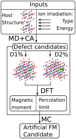
Figure 1: Computational scheme for the prediction of artificial functional magnetic materials. It takes as inputs the atomic structure of a host material and the ion type and energy range of the ion irradiation. In a first step, molecular dynamics (MD) simulations and cluster analysis (CA) algorithms yield possible defect structures and their corresponding creation probabilities, likely to be formed during the ion irradiation process. The resulting defective structures are used as input for DFT electronic structure calculations, giving the magnetic ground state and the percolation limit for each defect type. Finally, using the results of all calculations and applying Monte Carlo (MC) methods, a magnetic phase diagram is constructed, which indicates the irradiation parameters likely to create an artificial FM.

Taking the resulting structures of the defective host material as input for spin-polarized DFT calculations, allows us to save substantial computational effort and gives much more realistic results. Building on these remarks, we propose the computational scheme depicted in Figure 1, taking as input the atomic structure of a host material, the type and energy of the ion irradiation, from which potential defective structures and their creation probabilities are obtained using MD simulations and CA algorithms. DFT electronic structure calculations are then performed for the resulting defective structures and their magnetic ground state is determined. For defects yielding a non-zero magnetic moment, the percolation limit is estimated. Finally, taking into account ion energy loss in the irradiated host material and the defect formation probabilities predicted by the MD simulations, a magnetic phase diagram can be constructed using Monte Carlo (MC) methods. From this phase diagram, quantitative predictions of the total magnetic moment, the magnetic volume and magnetization can be extracted.

III High Energy Ion Irradiation in SiC

To validate the predictions of the computational scheme, we first calculate the magnetic phase diagram of 6H-SiC, resulting from the irradiation with high energy ($E_{\mathrm{ion}}=140$ keV) Ne ions and compare the predicted magnetization values with those measured experimentally and published by Li and coworkers [20]. In the following sections we aim to give a step-by-step example of the calculations involved in constructing the magnetic phase diagram and extracting quantitative predictions for the emerging FM phase.

III.1 Molecular Dynamics Collision Cascade Simulations

To find the defects produced in 6H-SiC resulting from high energy ion irradiation, we performed a total of 9600 collision cascade simulations in 6H-SiC using the LAMMPS MD code [21, 22, 23]. The interatomic interactions were modeled using Tersoff/ZBL empirical potentials, as described by Devanathan et al. [24] and used previously for similar simulations [25]. To compute the collision cascades, systems of $20\times 20\times 20$ unit cells (corresponding to 96000 atoms) with periodic boundary conditions were constructed. The unit cell parameters were set as $a=b=3.095$ Å, $c=15.185$ Å, $\alpha=\beta=90^{\circ}$, $\gamma=120^{\circ}$. Twelve initial structures were equilibrated in the microcanonical (NVE) ensemble for 10-21 ps, respectively, with a timestep of 1 fs at $T=300$ K. One Si atom and one C atom located at the center of the simulation cells were selected as primary knock-on atoms (PKA). Their initial kinetic energy was then set to values in the range 5 eV-200 eV by fixing the initial velocity along 10 different directions sampled from a cone with main axis along the (001) crystal direction and an aperture of $60^{\circ}$ (see Figure 2).

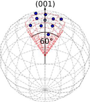
Figure 2: PKA directions sampled in the conical cut of the unit sphere, with aperture $60^{\circ}$ and axis along (001) crystal direction. Blue dots indicate the 10 initial directions used in the collision cascade simulations.

After setting the initial kinetic energy of the PKA atom, the systems were let to evolve in three phases, with timesteps of 0.01 fs, 0.1 fs and 1 fs for 0.1 ps, 1 ps and 10 ps, respectively, in order to capture the whole ballistic dynamics of the collision cascades.

The resulting collision cascade trajectories were then analyzed using the Ovito library. Single point defects (vacancies, interstitials, antisites) were identified using a Wigner-Seitz decomposition of the initial and final structure. Defect clusters were then identified using a clustering algorithm with a length cutoff of 2.5 Å, yielding the number of defect types created during each of the simulated collision cascades. The large degree of statistical sampling (120 simulations per PKA type and energy) allowed us to determine average defect creation rates, which are shown in Figure 3 for the C and Si PKAs in the energy range 5 eV to 200 eV. We find a displacement threshold of $E_{d}=25$ eV and $E_{d}=40$ eV for the C and Si PKA, respectively, in agreement with previous reports [25].

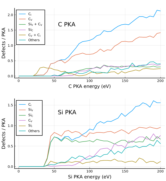
Figure 3: Defect creation rates in 6H-SiC obtained from collision cascades simulated by molecular dynamics methods for C and Si PKAs in the energy range 5 eV to 200 eV. The five most prevalent defect types are shown, all other defects are grouped together. C_I: carbon interstitial; C_V: carbon vacancy; Si_I: silicon interstitial; Si_V: silicon vacancy; Si_C: silicon antisite.

The most prevalent defects are the C interstitial (C_I), C vacancy (C_V), Si vacancy (Si_V), Si antisite (Si_C) and the di-vacancy (Si_V + C_V). We note that the creation rates shown in Figure 3 are given as average number of defects created per PKA event of a certain kinetic energy and type. In general, incident ions collide with one or more lattice ions, transferring some of their kinetic energy to the PKA. For a complete picture of the defect creation process, we need to determine the energy and spacial distribution of PKA events, created by energetic ions. But first, we need to identify those defects that carry non-zero magnetic moment and determine the sign and range of their exchange interactions.

III.2 Spin properties of the di-vacancy and Si vacancy in 6H-SiC

The spin properties of both the di-vacancy and the Si-vacancy in SiC have been extensively investigated due to their potential use as spin-defect qubits, both theoretically [26, 27, 28, 29, 30, 31] and experimentally [32, 33, 20, 34, 28, 29, 35, 31, 36]. According to spin-density functional theory calculations, the spin states and interactions strongly depend on the charge state of the defects [26, 34, 27, 29]. While the negatively charged Si vacancy has a spin-3/2 ground state, the neutral and higher charge states are not spin-polarized [26, 33]. The neutral and negatively charged di-vacancies have a spin-1 ground state [37, 27, 29]. In both defects, the calculated spin densities indicate that the polarization originates from localized states at the C atoms surrounding the Si vacancy.

Wang et al. investigated the exchange coupling between charged di-vacancies as a function of the defect distance [29] and found that the negatively charged di-vacancies couple ferromagnetically at distances 10-18.5 Å, corresponding to a percolation threshold of $\sim 1$ at.%.

III.3 Binary Collision Monte Carlo Simulations

Out of all defects predicted in the collision cascade simulations, the Si and di-vacancy are the most promising candidates to induce a long-ranged magnetically ordered phase in 6H-SiC, as they both carry non-zero magnetic moment, tend to couple ferromagnetically and both Si and C vacancies are created with a high probability (see Figure 3) in the collision cascades.

In order to relate the defect creation rates obtained from the MD collision cascade simulations to ion irradiation experiments, we need to determine the energy and spacial distribution of PKA events resulting from the collision of high energy ions with the SiC lattice atoms. We obtain this using SRIM [38, 39], a widely used binary collision Monte Carlo code, that simulates the stopping and range of ions in matter by assuming the target material is amorphous. In the full collision simulation mode, SRIM takes as input the number of ions to simulate, their type and kinetic energy, the target material composition and density, the displacement threshold of each target atom type and outputs a list of PKA collision events, including the transferred kinetic energy and the position.

To be able to compare our computational predictions to the experimental data published by Li and coworkers [20], we performed SRIM simulations of $10^{5}$ Ne⁺ ions at $E_{\mathrm{ion}}=140$ keV, incident on amorphous SiC, setting the displacement thresholds of the C atoms to $E_{d}=25$ eV and that of Si to $E_{d}=40$ eV, according to our MD simulations (see Figure 3). We analyzed the resulting PKA events using a histogram method with a bin size of 5 eV for the PKA energy, matching the energy resolution of our MD simulations. The PKA energy and depth (along the irradiation axis) distribution is shown for the two PKA types in Figure 4. In both cases, the maximum of the distribution lies around 40-50 eV and at a depth of 160 nm below the surface. The maximum range of the Ne⁺ ions is 260 nm. We note that, even though the initial kinetic energy of the ions was set to 140 keV, more than 90 % of the PKA events occur at an energy below 200 eV, indicating that the ions transfer most of their kinetic energy to the electronic system of the target material before undergoing binary collisions with the target nuclei.

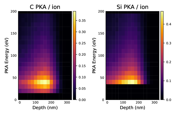
Figure 4: PKA event distribution for 6H-SiC irradiated with Ne ions at $E_{\mathrm{ion}}=140$ keV, calculated by binary collision Monte Carlo simulations using SRIM. The number of resulting primary knockon atom (PKA) events per incident ion is shown on the color scale (right axis) for C and Si PKAs as a function of the depth along the (001) crystal direction (horizontal axis) and the PKA energy (left axis).

III.4 Quantitative predictions and experimental validation

Combining the results of the MD and SRIM simulations, we calculated the densities of all defect types found in the MD simulations, as a function of ion fluence in the range 0-$5\times 10^{14}$ cm^-2 (see Figure 5). Pairs of single C and Si vacancies, created in close proximity were counted towards the di-vacancy density (Figure 5(b)) and the degree of amorphization (Figure 5(a)) was defined as the total number of defects per lattice atom. As the creation rate of C vacancies is significantly larger than that of Si vacancies, the resulting density of isolated Si vacancies is negligible and we will therefore only take into account the di-vacancy defect in our further discussion.

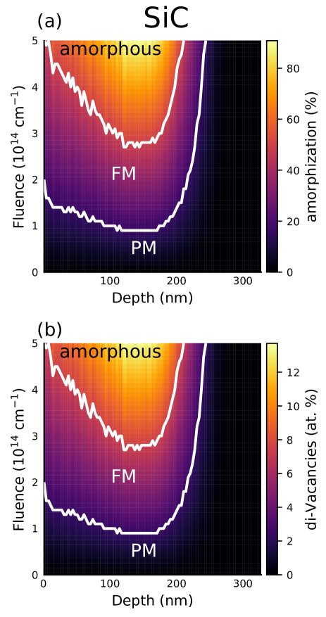
Figure 5: Magnetic phase diagram of 6H-SiC, irradiated with Ne ions at $E_{\mathrm{ion}}=140$ keV. FM: ferromagnetic, PM: paramagnetic. The degree of amorphization (a) and concentration of di-vacancies (b) are shown on the color scales (right axis) and as a function of depth along the (001) crystal direction (horizontal axis) and the irradiation fluence (left axis).

Taking into account a percolation threshold of 1 at.% for the di-vacancy defect [29], we identify the threshold ion fluence required to induce long-ranged FM order along the irradiation direction, as indicated in Figure 5 by the lower white line. Below this line, at low ion fluences, the defect density is too low to create an artificial FM phase and the material is paramagnetic. Above the line, at high enough fluences, a magnetic percolation transition occurs and a FM phase emerges.

As the spin polarization of the di-vacancy defect originates from the C atoms surrounding the Si vacancy, it appears plausible that a high degree of amorphization could destroy the FM phase. We have therefore calculated a second threshold fluence, at which the degree of amorphization along the irradiation direction reaches 50 %, as indicated by the upper white line in Figure 5. Above this threshold, at least two of the four C atoms surrounding the Si vacancy are displaced on average.

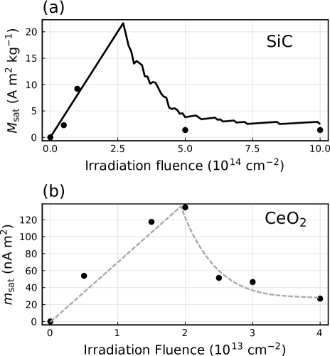
Figure 6: (a) Saturation magnetization of the ferromagnetic signal as a function of the ion irradiation fluence in a 6H-SiC single crystal sample irradiated with Ne⁺ ions at $E_{\mathrm{ion}}=140$ keV (data reproduced from [20]); (b) Saturation magnetic moment of a CeO₂ bulk sample, irradiated with Xe⁺ ions at $E_{\mathrm{ion}}=200$ MeV (data reproduced from [40]). The magnetic properties were measured after each irradiation step. The solid line in (a) show the calculated magnetization as described in the text; in (b) the line is just a guide for the eye. All measurements were done at room temperature.

These two boundaries define a volume, in which a FM phase emerges. By integrating over all defect magnetic moments in this volume, we obtain the saturation magnetization of the FM phase. This is shown as a solid line in Figure 6(a), as a function of the irradiation fluence. Up to a fluence of $2.5\times 10^{14}$ cm^-2, the magnetization increases linearly, as more defects are created. At higher fluences, the amorphization threshold is reached in a large portion of the magnetic volume and the magnetization rapidly decreases.

In order to compare our theoretical predictions with the experimental data published by Li et al. [20], we calculated the saturation magnetization from the total magnetic moment data measured using SQUID magnetometry by using the sample area and the depth of the magnetic phase resulting from our simulations. The resulting magnetization values are indicated in Figure 6(a) as bullets. The magnetization observed experimentally first increases with the Ne ion fluence and decreases at large enough fluences, matching our theoretical predictions quantitatively.

The authors suspected that the amorphization could play a role in the disappearance of the FM signal in their samples at larger fluences [20]. Our simulations confirm that the amorphization of the host lattice is the major limiting factor for the development of a dense FM phase in SiC. This might also be the case in other materials, where artificial FM phases have been created using ion irradiation. Detailed experimental data showing the evolution of such a FM phase as a function of the ion fluence is scarce. Shimizu et al. measured the magnetic properties of CeO₂ single crystals irradiated with Xe⁺ ions at $E_{\mathrm{ion}}=200$ MeV using SQUID magnetometry [40]. Figure 6(b) shows the evolution of the total saturation magnetic moment of an emerging FM phase in CeO₂, as a function of the ion fluence. There, the magnetic moment follows the same qualitative trend: It first increases rather linearly and at a fluence $>2\times 10^{13}$ cm^-2, it decreases.

IV Low Energy Ion Irradiation in Anatase TiO₂

Most experimental investigations of artificial FM phases emerging upon ion irradiation reported in the literature were performed at high ion energies $\geq 100$ keV. This results in a rather large ion penetration depth and as we showed in the previous section, the evolution of the artificial FM phase is limited by the amorphization of the host lattice. In this section, we present results of our systematic experimental investigation of a FM phase emerging in anatase TiO₂ hosts upon low energy Ar⁺ ion irradiation ($E_{\mathrm{ion}}\leq 1$ keV).

IV.1 Experimental Methods

Amorphous TiO₂ thin films were grown on SrTiO₂ substrates by ion beam sputter deposition [41]. Here a beam of low-energy Ar ions is directed onto a Ti target. Due to momentum and energy transfer, target particles get sputtered and condense on a substrate. Additionally oxygen background gas was provided such that TiO₂ thin films were formed. Ion energy, ion current, and ion incidence angle were 1000 eV, 7 mA, and 30^∘, respectively. The substrates were placed at a polar emission angle of 40^∘ relative to the target normal. The volumetric flow rate of Ar primary gas was 3.5 sccm and of O₂ background gas 2.0 sccm, which resulted in a total working pressure of $6\times 10^{-3}$ Pa. More details are given in Ref. [42]. The films have a thickness of 40 nm. After annealing at 500^∘ C in air for 1h, the films crystallize in the anatase phase with the film surface normal along the (001) crystal direction, as confirmed by XRD measurements (see Figure 7).

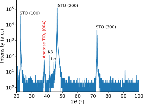
Figure 7: X-ray diffraction measurements of the crystallized anatase TiO₂ films grown on SrTiO₃ (100) substrates. The data shown here were obtained from sample S1000 after the last irradiation step.

Three thin film samples with a surface area of $5\times 5$ mm² were selected for the ion irradiation experiments. Each sample was then irradiated with Ar⁺ ions at $E_{\mathrm{ion}}=200$ eV (“S200”), 500 eV (“S500”) and 1000 eV (“S1000”), respectively, using a custom-built DC plasma chamber. The ion current was measured through a gold frame surrounding the sample during the irradiation process and was used to calculate the fluence.

The magnetic properties of each sample were characterized before and after each irradiation step using a commercial SQUID magnetometer (Quantum Design MPMS XL) using the reciprocating sample operation (RSO) mode. In order to ensure the comparability of the results after each irradiation step, great care has been taken to reduce as much as possible any source of contamination to the samples and the same protocol and schedule was maintained throughout the experiment. The samples were clamped in a plastic straw (as shown in Figure 10(b) in [43]), allowing to measure the magnetic responses to a magnetic field applied perpendicular and parallel to the film surface. The total magnetic moment of the sample was recovered from the raw SQUID voltage signal using a point dipole approximation. The finite sample size has been corrected for using methods described in Ref. [43], by applying a correction factor to the total moment (in-plane: 0.969296, perpendicular: 1.015966). For magnetic hysteresis loop measurements, $m(B)$, the magnetic field was first reduced from 0.1 T to nominally zero in oscillating mode, followed by a magnet quench to minimize the remanent field. In addition, the solenoid hysteresis was corrected for using a calibration measurement, as described in detail in [43]. For temperature dependent measurements, $m(T)$, the sample temperature was first set to $T=380$ K, followed by the same magnetic field reset procedure. After cooling the sample down to $T=2$ K, a constant magnetic field was set and the zero field cooled (ZFC) curve was measured while heating up to $T=380$ K followed by the field cooled (FC) measurement. At each temperature step, we waited for 60 seconds to allow the sample to reach thermal equilibrium prior to the measurement.

To recover the relevant magnetic hysteresis parameters from the experimental data, we use the following model:

$$m(B)=\chi B+\frac{2m_{s}}{\pi}\arctan\left[\frac{B\pm B_{c}}{B_{c}}\tan\left(\frac{\pi m_{r}}{2m_{s}}\right)\right],$$ (1)

where $\chi$ accounts for a linear contribution to the susceptibility, including a diamagnetic response from the substrate and a paramagnetic response at room temperature and moderate fields, $m_{s}$, $B_{c}$ and $m_{r}$ are the saturation moment, coercive field and remanent moment of a hysteretic response.

After the measurements of sample S500, and before measuring the other two samples, we had to adjust the “SQUID tuning parameters” (drive power and frequency) as the SQUID was slightly detuned, resulting in a significant reduction of the signal noise.

IV.2 Magnetic phase diagram

To understand the emergence of an artificial FM phase in TiO₂ due to low energy ion irradiation, we used the same computational scheme as for the high energy case, outlined in the previous section. Robinson et al. [44] performed detailed molecular dynamics simulations of collision cascades in anatase TiO₂, due to low energy ion irradiation and calculated the probability of resulting defect structures, as shown in Figure 2, for collision cascades resulting from Ti and O primary knock-on atoms (PKA), using a very similar method to ours. At PKA energies near the displacement threshold, $E_{d}=39$ eV for Ti PKAs and $E_{d}=19$ eV for O, the primary defects created are the di-Frenkel pair (dFP; 40% of Ti PKAs), consisting of two Ti atoms displaced into interstitial sites leaving behind two vacancies and the oxygen vacancy (O_v; 50% of O PKAs) (see Figure 2(a,c)).

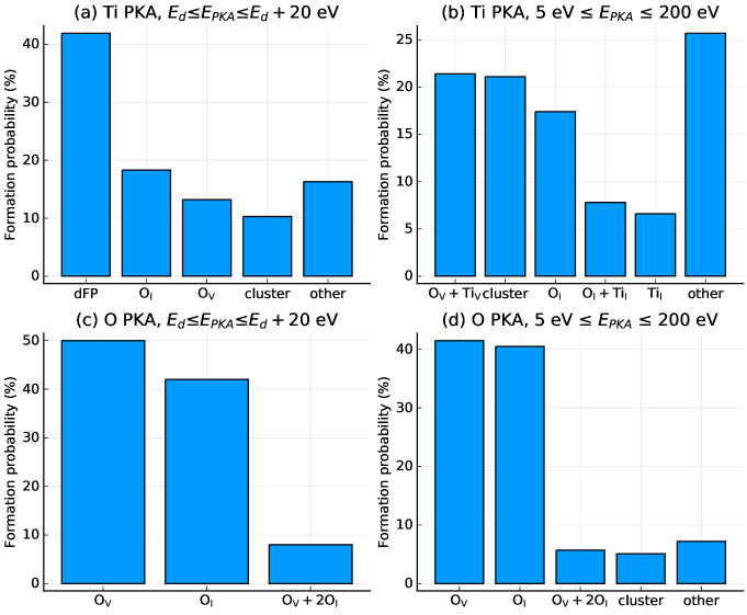
Figure 8: Defect formation probabilities at primary knockon (PKA) energies $E_{\mathrm{PKA}}$ near the displacement threshold $E_{d}$ (a,c) and in the range $5-200$ eV (b,d) for Titanium (a, b) and Oxygen (c, d) PKAs. Complexes containing more than four defects are categorized as “cluster”, the group labeled “other” contains defects with less than 5% formation probability. Data taken from Ref. [44].

Both the dFP [45] and O_v [46] defects in anatase TiO₂ have been investigated previously using DFT calculations and found to carry a magnetic moment of $2\mu_{B}$ and $1\mu_{B}$, respectively. When their concentration reaches $\sim 5$% in the bulk, the magnetic moments start to couple ferromagnetically and undergo a magnetic percolation transition. A long-ranged ordered phase emerges and persists even above room temperature [45]. According to reports from Stiller et al., dFP defects are mostly responsible for the emergence of a FM phase in anatase TiO₂ irradiated with low energy Ar⁺ ions [45]. The O_v defect was found to play a role in magnetic TiO₂ doped with Cu [46].

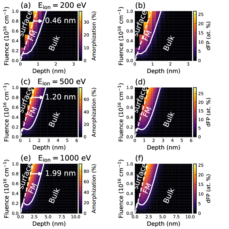
Figure 9: Magnetic phase diagram for the artificial FM created in anatase TiO₂ by Ar⁺ ions at $E_{\mathrm{ion}}=200$ eV (a,b), $E_{\mathrm{ion}}=500$ eV (c,d) and $E_{\mathrm{ion}}=1000$ eV (e,f). The color scale (right axes) shows the degree of amorphization (a,c,e) and the density of dFP defects (b,d,f), along the irradiation direction (lower axes) and as a function of the irradiation fluence (left axes). The solid white lines separate the regions with high enough defect concentration to form a ferromagnetic phase (FM) from those with low defect concentration forming a paramagnetic phase (PM) and indicates the percolation transition. The dashed white lines indicate the shift of the sample surface due to sputtering. At fluences $>4\times 10^{15}$ cm^-2, the thickness of the FM phase is stable, as indicated by the arrows in (a,c,e). The visible steps in the color maps are due to the discretization of the depth, which has a step size of $0.25c=2.4$ Å, corresponding to the anatase layer spacing in the (001) crystal direction.

Using SRIM simulations for Ar⁺ ions at $E_{\mathrm{ion}}=200$ eV, $500$ eV and $1000$ eV, and taking into account the defect creation probabilities (Figure 8), a magnetic phase diagram can be constructed. At low energies, the sample volume affected by the incident ions is much smaller than in the high energy case and the effect of surface sputtering has to be taken into account. SRIM allows to calculate the sputtering rate. We find values of 1.1, 1.5 and 2.3 nm / ($10^{16}$ ions / cm²) at ion energies of 200 eV, 500 eV and 1000 eV, respectively.

Figure 9 shows the dFP density and degree of amorphization as a function of the Ar ion fluence for the three ion energies considered in this study. Due to sputtering, the amorphization of the host lattice has a much smaller effect, as the thin amorphous surface layer is constantly removed. This is indicated by a dashed line in Figure 9. The solid line indicates the magnetic percolation transition between unordered (paramagnetic) and FM phases.

At fluences $>4\times 10^{15}$ cm^-2, the defect creation and sputtering processes are at equilibrium. The volume and defect densities of the emerging FM phase stay constant over the whole fluence range. The equilibrium volume depends on the ion energy, as indicated by the thickness of the FM regions along the irradiation direction in Figure 9. At $E_{\mathrm{ion}}=200$ eV, the emerging FM layer grows to an equilibrium thickness $d_{\mathrm{FM}}=4.6$ Å, corresponding to $0.48c$ ($c=9.51$ Å, the Anatase lattice constant). At $E_{\mathrm{ion}}=500$ eV we find an equilibrium thickness $d_{\mathrm{FM}}=12.0$ Å ($=1.26c$) and at $E_{\mathrm{ion}}=1000$ eV, $d_{\mathrm{FM}}=19.9$ Å ($=2.09c$). The anatase unit cell consists of four layers, stacked along the (001) crystal direction. Therefore, the emerging FM phase is expected to be restricted to the first 2, 4 and 8 layers of the host lattice, respectively.

IV.3 Experimental observation of the emerging FM phase in Anatase TiO₂

Figure 10(a) shows two typical hysteresis curves, measured at room temperature and after sample S1000 had been irradiated with a fluence of $0.6\times 10^{16}$ cm^-2 (blue) and $8.7\times 10^{16}$ cm^-2 (orange). After subtracting the linear diamagnetic background (Figure 10(b)), a hysteretic FM signal clearly appears, showing a magnetic moment at saturation $m_{\mathrm{sat}}$ that increases with ion fluence (hysteresis curves at all irradiation fluences are shown in Figures S1-S3 in the supporting information). Figure 10(c) shows the zero-field cooled (ZFC) and field cooled (FC) curves, measured at an irradiation fluence of $18.3\times 10^{16}$ cm^-2, in the temperature range 2-380 K and at an applied magnetic field of $B=0.05$ T. The opening between the ZFC and FC curves is a clear sign of a FM phase.

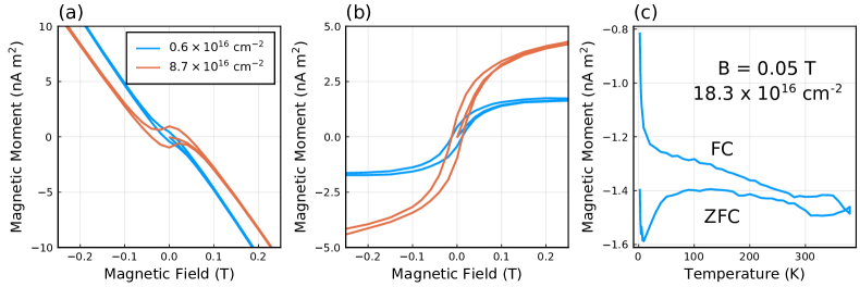
Figure 10: (a,b) TiO₂ thin film irradiated with $0.6\times 10^{16}$ cm^-2 (blue) and $8.7\times 10^{16}$ cm^-2 (orange) Ar⁺ ions at $E_{\mathrm{ion}}=1000$ eV. (a) Hysteresis loop showing total magnetic moment as a function of applied magnetic field at $T=300$ K. (b) Hysteresis loop after subtracting a linear diamagnetic background. The magnetic field was applied parallel to the film surface. (c) Zero-field cooled (ZFC) / field cooled (FC) curve, measured at $B=0.05$ T for sample S1000 at an irradiation fluence $18.3\times 10^{16}$ cm^-2.

By systematically measuring the magnetic hysteresis of the samples as a function of the irradiation fluence, we can gain some insight into the evolution of the emerging FM phase. Figure 11(a) shows the total magnetic moment at saturation at $T=300$ K, $m_{\mathrm{sat}}$, after subtracting the linear diamagnetic background, as a function of the irradiation fluence, for the three samples S200, S500 and S1000. The values of $m_{\mathrm{sat}}$ have been obtained by fitting the hysteresis curves with Equation (1). The background signal $m_{0}$, measured in each sample before any irradiation was subtracted. The magnetization $M_{\mathrm{sat}}$ was calculated from the measured total moment $m_{\mathrm{sat}}$ taking into account the equilibrium volume of the magnetic phase predicted from the phase diagram (Figure 9).

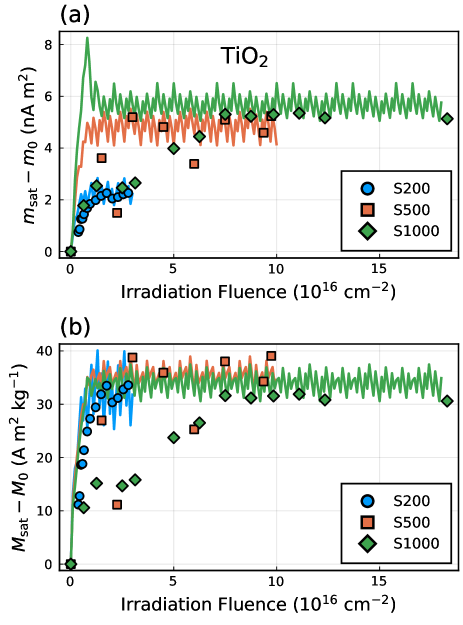
Figure 11: Magnetic moment $m_{\mathrm{sat}}$ (a) and magnetization $M_{\mathrm{sat}}$ (b) at saturation of the ferromagnetic signal, measured at room temperature as a function of the ion irradiation fluence, in the three TiO₂ thin film samples, S200 ($\bullet$), S500 ($\blacksquare$) and S1000 ($\blacklozenge$). The background signal, $m_{0}$ ($M_{0}$) measured before any irradiation has been subtracted from the experimental data. The solid lines show the magnetic moment (magnetization) values predicted from our theoretical calculations (Figure 9).

We first observe that the moment at saturation increases with increasing total irradiation fluence and saturates at high fluences. This is expected, as increasing the irradiation fluence also increases the density of dFP defect complexes until the defect creation and sputtering processes reach equilibrium, in agreement with the phase diagram (Figure 9). The saturation magnetization of all three samples reaches values of the order of 35 Am²kg^-1, which corresponds to a mean dFP concentration of $\sim 17$ at. % or one dFP per unit cell.

By numerically integrating the dFP concentration found in our calculations over the volume of the FM phase in Figure 9 and taking into account the magnetic moment ($2\mu_{B}$) of each dFP defect, we can calculate the expected magnetization and total moment of the samples as a function of the irradiation fluence. The result is shown in Figure 11 as solid lines. The oscillations are numerical artifacts due to the discretization of the phase diagram. At the lowest ion energy (sample S200), our predictions show excellent agreement with the experimental data. The predicted equilibrium magnetization at high irradiation fluences of all three samples also agrees very well with our measurements. The evolution of the magnetization of sample S1000 to the equilibrium value, on the other hand, does not agree well with our calculations, that predict a much steeper approach to equilibrium. In fact, it appears like the saturation moment of sample S1000 first follows the same evolution as sample S200 (Figure 11) and then slowly increases to the equilibrium value.

IV.4 The magnetic percolation process

We have seen in Figure 9 that the FM phase emerges in an ultrathin region of thickness between 2 and 8 anatase layers. To better understand the evolution of these ultrathin FM layers, it is instructive to take a closer look at the magnetic percolation process, i.e. the transition from isolated local magnetic moments to a long-ranged ordered phase upon increasing the defect density.

A system of dilute defects in a host lattice that interact magnetically on a finite length scale can be described using the framework of percolation theory [47, 48]. In the site-percolation model, sites on the host lattice can be occupied by a defect and one can associate a probability $p$ with the occupation of a site. At $p=0$, no defects are present in the system and at $p=1$, all sites are occupied by a defect. This probability is naturally related to the defect density in the system through the density of possible sites that can host a defect.

The length scale of the magnetic interaction, namely the exchange coupling, determines whether two occupied sites are linked: Two occupied sites that are close enough to each other to interact ferromagnetically through the exchange interaction form a percolation domain. The magnetic moments associated to each site belonging to one percolation domain are correlated, while those associated to different percolation domains behave independently.

The site-percolation model describes a second order geometrical phase transition, that occurs at a critical occupation probability $p_{c}$. At $p<p_{c}$, in the subcritical regime, small isolated percolation domains form. The microscopic magnetic moments within each of these percolation domains are aligned parallel to each other due to the ferromagnetic coupling, but their orientation is arbitrary. The summed magnetic moment of each domain can be treated as one large paramagnetic center and the system is in a super-paramagnetic phase. At $p>p_{c}$, in the supercritical regime, one large percolation domain exists that spans over the whole system volume. This domain is called the percolation continent and exhibits the features of a ferromagnet, such as a spontaneous magnetization.

At criticality, when $p\sim p_{c}$, the percolation continent emerges and the defective host system becomes ferromagnetic. As with all second order phase transitions, the percolation transition can be described by an order parameter, namely the probability $P_{\infty}$, that a random defect belongs to the percolation continent. Near criticality, the evolution of the order parameter follows a power law of the form

$$P_{\infty}\propto(p-p_{c})^{\beta},$$ (2)

with a universal critical exponent $\beta$, that only depends on the dimensionality of the system.

We simulate the magnetic percolation process in a grid of $200\times 200$ anatase TiO₂ unit cells and a thickness of 1, 2 and 3 layers, enforcing periodic conditions on the lateral boundaries. For comparison, we perform the same simulations in a $200\times 200\times 200$ unit cell grid, enforcing periodic boundary conditions in all three directions for a bulk system. Magnetic dFP defects are randomly distributed throughout the grids, varying the total defect concentration. Only nearest neighbor interactions between dFP defects are taken into account, such that two nearest neighbor cells, each containing a dFP defect, interact ferromagnetically and form a percolation domain. Figure 12(a) shows the size of the largest of the domains, the percolation continent, normalized to the total size of the grid. Figure 12(b) shows the number of independent percolation domains within the grid, as a function of the dFP defect concentration, normalized to the total number of cells in the grids.

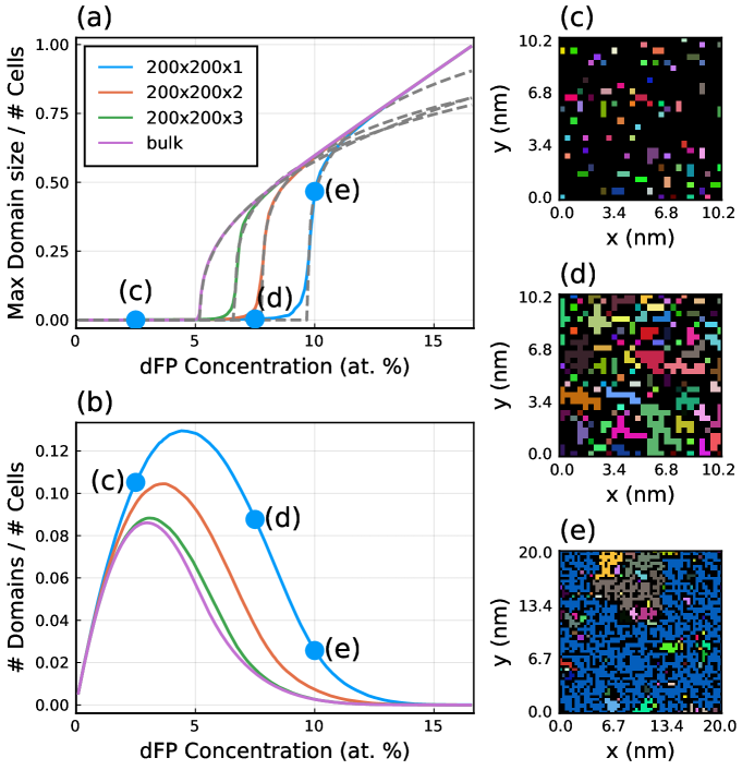
Figure 12: Magnetic percolation process in $200\times 200\times Z$ ($Z=1,2,3$ and bulk) unit cell TiO₂ slabs for varying dFP concentrations. Nearest neighbor cells containing a dFP interact and form percolation domains. Varying the dFP concentration, three regimes can be seen: at low concentration ($<5$ at. % in the monolayer), the sample is paramagnetic and the percolation domains are small. In the intermediate regime (5-9 at. % in the monolayer), the magnetic dFP defects start to interact and the domains grow rapidly in size. At the percolation threshold, 9 at. %, 7.5 at.%, 6 at.% and 5 at. % in the mono-, bi-, trilayer and the bulk system, respectively, the domains merge and form a large percolation continent. The size of the percolation continent is shown in (a) as a function of the dFP concentration; (b) shows the number of percolation domains (normalized by the total number of cells). (c)-(e) Examples of monolayer grids, in which individual domains are color-coded. Black cells correspond to non-magnetic cells, that do not contain any dFP defect. Regions of the same color correspond to percolation domains, in which each cell has at least one nearest neighbor cell containing a dFP. The defect concentration was set to 2.5 at. % (c), 7.5 at. % (d) and 10 at. % (e). These three examples are marked by blue dots in (a) and (b). The dashed lines in (a) correspond to the fits of Equation (2).

Varying the defect density, we see three regimes: at low concentration ($<5$ at. % in the monolayer), the sample is paramagnetic and the percolation domains are small (see Figure 12(c)). In the intermediate regime (5-9 at. % in the monolayer), the magnetic dFP defects start to interact and the domains grow rapidly in size (see Figure 12(d)). At the percolation threshold, 9 at. %, 7.5 at.%, 6 at.% and 5 at. % in the mono-, bi-, trilayer and the bulk system, respectively, the domains merge and the percolation continent grows rapidly until spanning over the whole grid (see Figure 12(e)). We note that at a dFP density of 17 at. %, which we found at equilibrium in Figure 11, the percolation continent has fully evolved and the order parameter $P_{\infty}=1$.

Table 1: Critical exponents $\beta$ obtained by fitting Equation (2) to the data shown in Figure 12(a).

# layers	$\beta$
1	$0.210\pm 0.007$
2	$0.220\pm 0.006$
3	$0.259\pm 0.007$
bulk	$0.417\pm 0.004$

Table 1 shows the critical exponents obtained by fitting the curves shown in Figure 12(a) to Equation (2). Experimentally, the magnetic percolation transition can be obtained by taking the remanent magnetic moment at zero applied magnetic field and at high temperatures. Indeed, at ion fluences below the percolation transition, the samples are expected to be (super-)paramagnetic and no remanence is expected above the blocking temperature. Near the percolation transition, when the percolation continent forms at a critical fluence $f_{c}$, the remanent magnetic moment should follow the same critical behavior as the order parameter $P_{\infty}$.

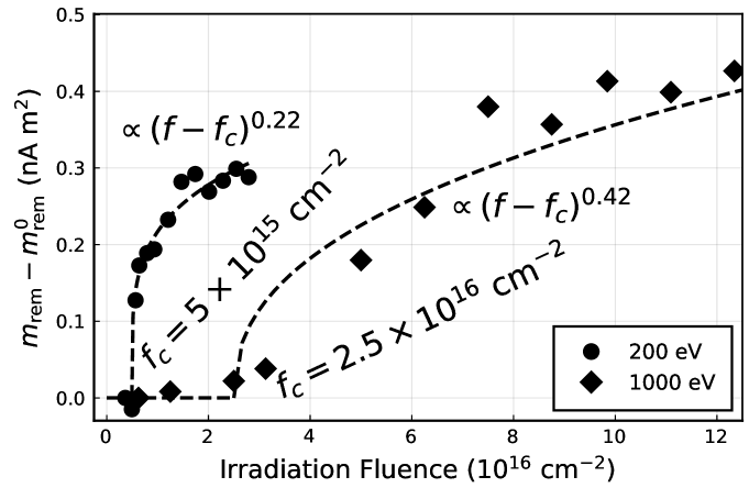
Figure 13: Remanent magnetic moment $m_{\mathrm{rem}}$ at zero field, measured at $T=300$ K after setting a magnetic field $B=5$ T, as a function of the irradiation fluence $f$. The background remanence $m_{\mathrm{rem}}^{0}$ of the unirradiated samples was subtracted. The symbols represent experimental data of samples S200 ($\bullet$) and S1000 ($\blacklozenge$). The dashed lines represent fits to $m_{\mathrm{rem}}\propto(f-f_{c})^{\beta}$, with the critical fluences ($f_{c}$) and critical exponents ($\beta$) as indicated.

Figure 13 shows the evolution of the remanent magnetic moment $m_{\mathrm{rem}}$ measured in samples S200 and S1000 as a function of the irradiation fluence $f$. By fitting the data to a power law ($m_{\mathrm{rem}}\propto(f-f_{0})^{\beta}$), we find critical fluences $f_{0}=5\times 10^{15}$ cm^-2 and $2.5\times 10^{16}$ cm^-2 for samples S200 and S1000, respectively. The resulting critical exponents are $\beta=0.22\pm 0.04$ and $0.42\pm 0.07$, respectively. Comparing these exponents to the theoretical values (Table 1), we see that the remanence observed in sample S1000 follows the critical behavior of a bulk 3D percolation transition, while sample S200 follows the critical behavior of a magnetic bilayer system. These results match very well with the aforementioned thickness of the FM phases (see Figure 9), that predicted the emergence of a magnetic bilayer in sample S200, while in sample S1000 the FM phase spans over 8 layers.

V Dimensionality and surface effects, emergence of a perpendicular magnetic anisotropy

Two dimensional long ranged magnetic order has long been thought to be impossible at finite temperatures, as stated by the Mermin-Wagner (MW) theorem [49]: In bulk 3D ferromagnets, the exchange interaction asserts a long range magnetic order up to the Curie temperature, $T_{C}$, where thermal fluctuations become strong enough to randomize the spin orientation. In 2D magnetic systems with isotropic exchange interaction, the dimensionality effect leads to an abrupt jump in the magnon dispersion and therefore strong spin excitations at any finite temperature, destroying the magnetic order. The presence of a strong uniaxial local magnetic anisotropy opens a gap in the magnon dispersion, counteracting the Mermin-Wagner theorem in 2D and restoring long range order. This has been demonstrated experimentally in ultrathin transition metal films [50, 51] and 2D magnetic van der Waals materials [52, 53, 10]. 2D magnetic structures are not only interesting from a fundamental physics perspective, but also regarding their possible applications in 2D spintronics, magnonics or spin-orbitronics [2, 53, 3, 1, 10]. In the following section, we shall show the role of the magnetic anisotropy and of the surface to stabilize the artificial FM phase at room temperature in TiO₂ hosts, even in two dimensions.

V.1 Measuring the magnetic anisotropy of the emerging FM phase in TiO₂ hosts

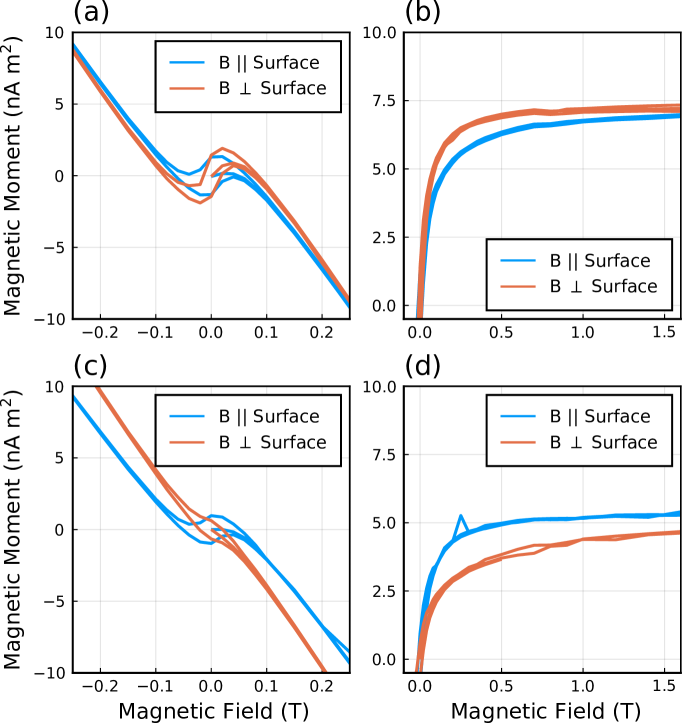
Figure 14: Magnetic hysteresis loops measured with the external magnetic field applied in the plane of the TiO₂ films (blue) and out-of-plane (orange), measured at $T=300$ K. The left panels show the total magnetic moment measured with the SQUID, the right panels show the ferromagnetic signal after subtracting the background diamagnetic and paramagnetic signals. Panels (a),(b) show the results obtained for sample S200 after irradiation with a fluence of $2.5\times 10^{16}$ cm^-2 and panels (c),(d) for sample S500 at a fluence of $6.0\times 10^{16}$ cm^-2.

Figure 14 shows measurements of the magnetic hysteresis loops obtained by applying an external magnetic field parallel to the film surface (blue) and perpendicular to the surface (orange) of the three TiO₂ samples. In panels (a,c), the raw signals are shown and a clear magnetic anisotropy is visible. After subtracting the linear diamagnetic contribution (Figure 14(b,d)), the total magnetic anisotropy energy (MAE) can be calculated as the area difference between the two curves. Here, we calculated the area difference by first fitting Equation (1) to the experimental data and integrating the result analytically. To compensate differences in the resulting saturation moments $m_{\mathrm{sat}}$ for the two field orientations, e.g. due to fitting error or finite sample size effects (see Section IV.A), we rescaled the values of $m_{\mathrm{sat}}$ and $m_{\mathrm{rem}}$, such that $m_{\mathrm{sat}}$ coincides. The sign is defined such that positive MAE indicates a magnetic easy in-plane direction, parallel to the film surface while a negative MAE indicates an out-of-plane easy axis. More details are given in the supporting information. At the selected irradiation fluences, sample S200 (panels (a,b)) shows a perpendicular magnetic anisotropy while sample S500 (panels (c,d)) shows an in-plane anisotropy.

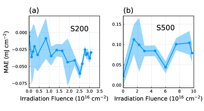
Figure 15: The magnetic anisotropy energy (MAE) obtained from the magnetic hysteresis curves measured after each irradiation step for the TiO₂ sample S200 (a) and S500 (b). The MAE is defined such that a negative value indicates an out of plane easy-axis (along the film surface normal), while a positive value indicates an easy in-plane magnetization direction (parallel to the film surface). The shaded area indicates the confidence margin within 5% significance level.

Figure 15 shows the total MAE as a function of the irradiation fluence, of the samples S200 (a) and S500 (b). In sample S200, where the thickness of the FM phase is estimated to only two layers of the host lattice, the MAE is negative throughout all irradiation fluences, indicating a magnetic easy axis normal to the film surface. In sample S500, the MAE is positive and its magnitude is roughly four times larger than that of sample S200. For sample S500, the magnetic phase diagram (Figure 9) predicts a FM phase spanning the first four layers of the film surface, i.e. twice as many as for sample S200, hinting towards the role of the surface in the emergence of a perpendicular magnetic anisotropy.

V.2 DFT electronic structure calculations of the defective TiO₂ surface

To understand the origin of the magnetic anisotropy shown in Figure 15, we performed DFT electronic structure calculations using the full potential linearized augmented plane wave (FLAPW) method implemented in the FLEUR code, including spin-orbit interaction and a Hubbard term $U=4.0$ eV, on a $3\times 3\times 1$ supercell of anatase TiO₂, containing one dFP defect (the defect labeled “di-FP1” in Ref. [45]). We used a planewave cutoff times muffin tin radius $K_{\mathrm{max}}\times a_{\mathrm{MT}}=7.0$. The atomic structure was relaxed using a $2\times 2\times 2$ k-point grid and the final charge and spin density was calculated using a $6\times 6\times 6$ k-point grid. Figure 16(a) shows the relaxed bulk atomic structure, with the two Ti interstitials colored in pink. The isosurface at a spin density of $0.005\mu_{B}a_{0}^{-3}$ is shown in yellow and is mainly located around the two interstitials and their neighboring Ti lattice atoms in the (010) plane, having $d_{xz}$ character, as confirmed by the density of states (Figure 16(a)). We find a total magnetic moment of $2\mu_{B}$/dFP defect. These calculations match well with those presented by Stiller et al. [45]. We also calculated the MAE from the total energy difference between the in-plane and out-of-plane magnetization state and find $\mathrm{MAE}=11$ $\mu$eV/atom with an (001) easy-plane in the bulk, as opposed to the out-of-plane easy axis found by Stiller et al [45].

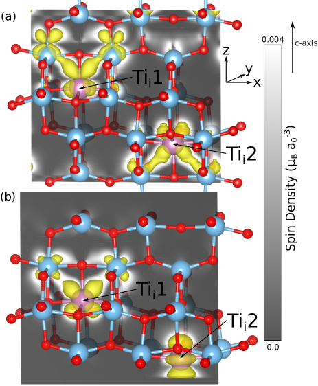
Figure 16: FLAPW-DFT calculations for (a) a 3x3x1 bulk anatase supercell and (b) a 3x3x1 supercell of the (001) anatase surface, each containing one dFP defect per supercell. The relaxed atom positions are represented by spheres (blue: Ti, red: O, purple: Ti_i). The isosurface at 0.005 $\mu_{B}a_{0}^{-3}$ spin density is shown in yellow. The spin density in the (010)-plane through the two interstitials is indicated by shades of gray according to the scale on the right.

We then calculated the electronic structure of the dFP defect at the (001) anatase surface, using a $3\times 3$ supercell containing four layers of anatase, as shown in Figure 16(b). Only the lower two layers were relaxed, while the upper two were held fixed at the bulk atomic positions. After structural relaxation, the surface layer shows displacements comparable to values found in the literature [54] ($\alpha=142^{\circ}$, Ti_5c–O_2c (short) $=1.813$ Å, Ti_5c–O_2c (long) $=2.010$ Å, Ti_5c–O${}_{3c}=1.941$ Å). As visible in Figure 16(b), the spin density (shown in yellow) has similar structure as in the bulk around the interstitial Ti_i1 on the second layer. On the first layer, on the other hand, the spin density at interstitial Ti_i2 changes strongly owing to the reduced coordination. There, the Ti 3d${}_{z^{2}}$ orbital is mainly spin polarized, as reflected by the DOS (Figure 17(b)). The magnetic anisotropy at the (001) surface results in an out-of-plane easy axis with a large $\mathrm{MAE}=-137$ $\mu$eV/atom.

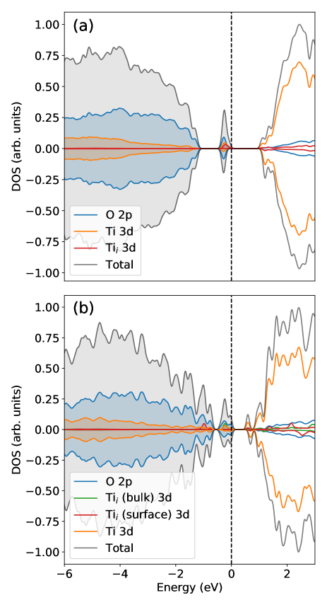
Figure 17: Density of states (DOS) (a) of the bulk anatase structure and (b) of the (001)-surface, each containing $5.5$% dFP. The total DOS is shown in gray; the partial DOS (PDOS) of O 2p states is shown in blue; the PDOS of Ti 3d states is shown in orange. In (a), the PDOS of the two equivalent interstitial 3d states is shown in red; in (b), the PDOS of the bulk (Ti_i1) and surface (Ti_i2) interstitials are shown in green and red, respectively.

These results together with the calculated defect distribution (Figure 9) explain the measured MAE (Figure 15): At low ion energy of $E_{\mathrm{ion}}=200$ eV (sample S200), the FM phase emerges in the first two layers at the film surface, resulting in a large negative MAE. At higher ion energies, the FM phase emerges in a larger volume and also has contributions from bulk states, which favor an in-plane easy-axis. Depending on the local distribution of the defects, either the surface or the bulk states dominate the total MAE.

VI Conclusions

The computational methods proposed in this work serve as a viable route toward the systematic discovery of new artificial functional magnetic materials that can be created experimentally by ion irradiation techniques. With a minimal amount of input parameters, the scheme provides excellent quantitative predictions in a large range of ion energies. The information gained from first principles helps to understand existing experimental results and notably solve the inherent problem of the experimental uncertainty regarding the magnetic volume, which has been a major source of controversy.

By revisiting experimental results from the literature of a FM phase emerging in SiC upon high energy ion irradiation and comparing them to our computational predictions, we found that the main process limiting the evolution of the artificial FM phase at high ion energies is the amorphization of the host lattice.

In the case of low ion energies, sputtering of lattice atoms at the surface plays an important role and limits the degree of amorphization, as we demonstrated experimentally in anatase TiO₂ hosts. When the defect production and sputtering processes reach an equilibrium, high defect densities (up to 17 at. %) can be created, which allows full magnetic percolation. We have shown that at low enough ion energies ($E_{\mathrm{ion}}=200$ eV in the TiO₂), ultrathin ferromagnetic films down to a magnetic bilayer can be created.

In the ultrathin artificial FM layers created in TiO₂ hosts, we have investigated the magnetic anisotropy and showed that a perpendicular magnetic anisotropy emerges, depending on the thickness of the magnetic phase. We could identify the origin of this PMA in the contribution of magnetic surface states, as shown by DFT calculations.

Appendix A Magnetic Hysteresis Curves

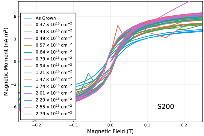
Figure 18: Hysteresis loops measured in the TiO₂ sample S200 at $T=300$ K after each Ar⁺ irradiation step. The linear diamagnetic background was subtracted.

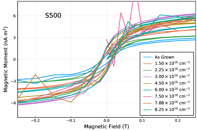
Figure 19: Hysteresis loops measured in the TiO₂ sample S500 at $T=300$ K after each Ar⁺ irradiation step. The linear diamagnetic background was subtracted.

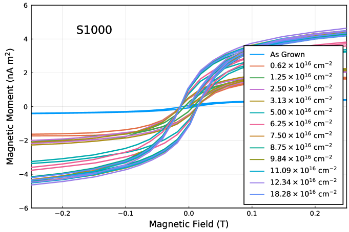
Figure 20: Hysteresis loops measured in the TiO₂ sample S1000 at $T=300$ K after each Ar⁺ irradiation step. The linear diamagnetic background was subtracted.

Appendix B Magnetic Anisotropy Energy

Figure 21 shows the magnetic anisotropy energy (MAE) of sample S200 and S500 as a function of the irradiation fluence. The MAE was obtained from magnetic hysteresis curves such as those shown for some example fluences. Hysteresis curves were measured once with the magnetic field applied in-plane (blue bullets) and perpendicular to the sample surface (orange bullets). Each curve was then fit using Equation (3)

$$m(B;m_{s},m_{r},B_{c})=\frac{2m_{s}}{\pi}\arctan\left[\frac{B\pm B_{c}}{B_{c}}\tan\left(\frac{\pi m_{r}}{2m_{s}}\right)\right],$$ (3)

to recover the saturation moment $m_{s}$, the remanent moment $m_{r}$ and the coercive field $B_{c}$. The magnetic energy was then calculated along the virgin curve as

$$E(m_{s},m_{r},B_{c})=\int_{0}^{B_{\mathrm{max}}}m(B;m_{s},m_{r},B_{c})\mathrm{d}B.$$ (4)

The integration cutoff $B_{\mathrm{max}}$ was set to 5 T. The MAE was then calculated as

$$MAE=\frac{1}{A}\left[E(m_{s}^{\parallel},m_{r}^{\parallel},B_{c}^{\parallel})-E(m_{s}^{\parallel},m_{r}^{\perp}m_{s}^{\parallel}/m_{s}^{\perp},B_{c}^{\perp})\right],$$ (5)

with $A$ the sample surface area. We note that the saturation and remanent moments obtained in the perpendicular configuration were rescaled, so that the two saturation moments match.

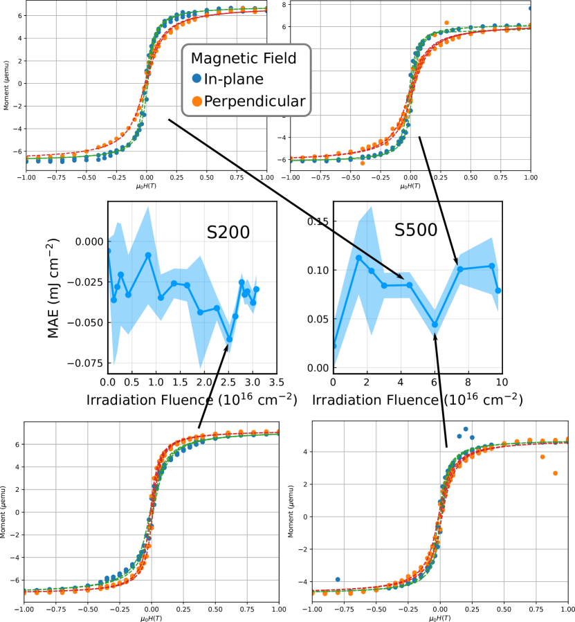
Figure 21: Hysteresis loops, measured at $T=300$ K with a magnetic field applied in-plane and perpendicular to the film surface, corresponding to the magnetic anisotropy energy (MAE) values marked by arrows. The dashed lines show the fits to Equation (1) in the main text. The method to obtain the MAE from the hysteresis curves is described in Section V.A of the main text.